
1
The Basics of ZPL
Like sequential computation with its C programming language and von Neumann model of computation explaining the performance of programs, parallel
computation needs a language calibrated to the CTA model. ZPL is the only such language.
2
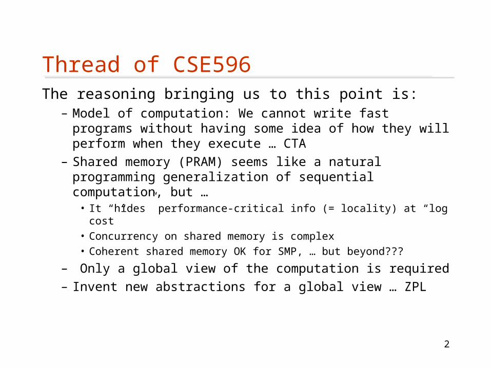
Thread of CSE596The reasoning bringing us to this point is:
– Model of computation: We cannot write fast programs without having some idea of how they will perform when they execute … CTA
– Shared memory (PRAM) seems like a natural programming generalization of sequential computation, but …
• It “hides” performance-critical info (= locality) at “log cost”• Concurrency on shared memory is complex • Coherent shared memory OK for SMP, … but beyond???
– Only a global view of the computation is required– Invent new abstractions for a global view … ZPL
3
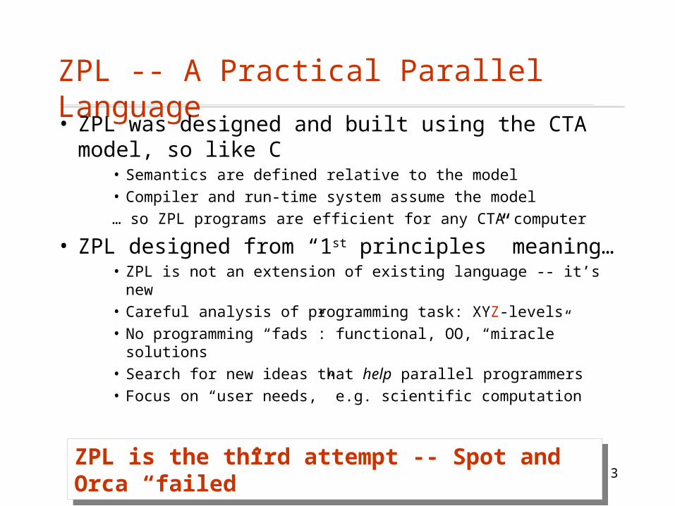
ZPL -- A Practical Parallel Language• ZPL was designed and built using the CTA
model, so like C• Semantics are defined relative to the model
• Compiler and run-time system assume the model
… so ZPL programs are efficient for any CTA computer
• ZPL designed from “1st principles” meaning…• ZPL is not an extension of existing language -- it’s new• Careful analysis of programming task: XYZ-levels
• No programming “fads”: functional, OO, “miracle” solutions• Search for new ideas that help parallel programmers
• Focus on “user needs,” e.g. scientific computation
ZPL is the third attempt -- Spot and Orca “failed” ZPL is the third attempt -- Spot and Orca “failed”

4
ZPL ...Is an array language -- whole arrays are manipulated
with primitive operations• Requires new thinking strategies --
• Forget one-operation-a-time scalar programming• Think of the computation globally -- make the global logic work
efficiently and leave the details to the compiler
• Is parallel, but there are no parallel constructs in the language; the compiler...
• Finds all concurrency• Performs all interprocessor communication• Implements all necessary synchronization (almost none)• Performs extensive parallel and scalar optimizations
5
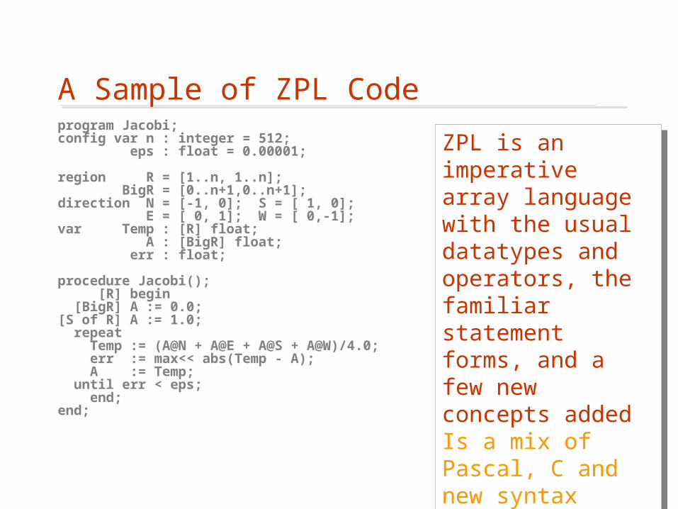
A Sample of ZPL Codeprogram Jacobi;config var n : integer = 512; eps : float = 0.00001;
region R = [1..n, 1..n]; BigR = [0..n+1,0..n+1];direction N = [-1, 0]; S = [ 1, 0]; E = [ 0, 1]; W = [ 0,-1];var Temp : [R] float; A : [BigR] float; err : float;
procedure Jacobi(); [R] begin[BigR] A := 0.0;
[S of R] A := 1.0;repeat Temp := (A@N + A@E + A@S + A@W)/4.0; err := max<< abs(Temp - A); A := Temp;until err < eps;
end;end;
ZPL is an imperative array language with the usual datatypes and operators, the familiar statement forms, and a few new concepts added Is a mix of Pascal, C and new syntax
ZPL is an imperative array language with the usual datatypes and operators, the familiar statement forms, and a few new concepts added Is a mix of Pascal, C and new syntax
6
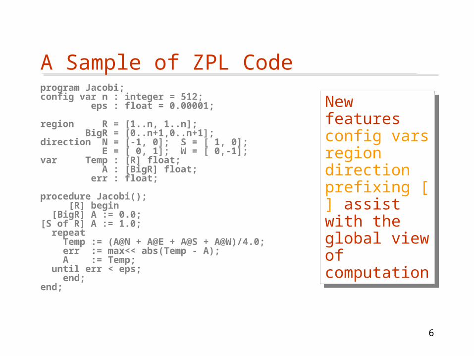
A Sample of ZPL Codeprogram Jacobi;config var n : integer = 512; eps : float = 0.00001;
region R = [1..n, 1..n]; BigR = [0..n+1,0..n+1];direction N = [-1, 0]; S = [ 1, 0]; E = [ 0, 1]; W = [ 0,-1];var Temp : [R] float; A : [BigR] float; err : float;
procedure Jacobi(); [R] begin[BigR] A := 0.0;
[S of R] A := 1.0;repeat Temp := (A@N + A@E + A@S + A@W)/4.0; err := max<< abs(Temp - A); A := Temp;until err < eps;
end;end;
New features config vars region direction prefixing [ ] assist with the global view of computation
New features config vars region direction prefixing [ ] assist with the global view of computation
7
Jacobi Iteration: How does it work?program Jacobi;config var n : integer = 512; eps : float = 0.00001;
region R = [1..n, 1..n]; BigR = [0..n+1,0..n+1];direction N = [-1, 0]; S = [ 1, 0]; E = [ 0, 1]; W = [ 0,-1];var Temp : [R] float; A : [BigR] float; err : float;
procedure Jacobi(); [R] begin[BigR] A := 0.0;
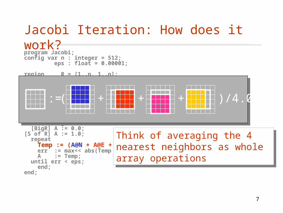
[S of R] A := 1.0;repeat Temp := (A@N + A@E + A@S + A@W)/4.0; err := max<< abs(Temp - A); A := Temp;until err < eps;
end;end;
Think of averaging the 4 nearest neighbors as whole array operations
Think of averaging the 4 nearest neighbors as whole array operations
:= ( + + + )/4.0;
8
Regions: A New Conceptprogram Jacobi;config var n : integer = 512; eps : float = 0.00001;
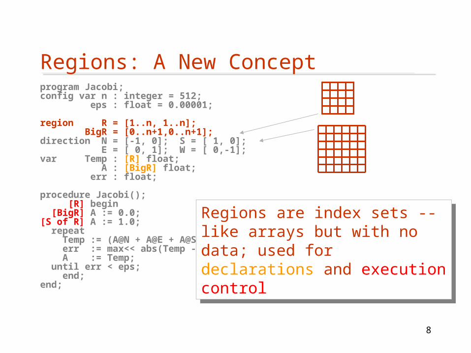
region R = [1..n, 1..n]; BigR = [0..n+1,0..n+1];direction N = [-1, 0]; S = [ 1, 0]; E = [ 0, 1]; W = [ 0,-1];var Temp : [R] float; A : [BigR] float; err : float;
procedure Jacobi(); [R] begin[BigR] A := 0.0;
[S of R] A := 1.0;repeat Temp := (A@N + A@E + A@S + A@W)/4.0; err := max<< abs(Temp - A); A := Temp;until err < eps;
end;end;
Regions are index sets -- like arrays but with no data; used for declarations and execution control
Regions are index sets -- like arrays but with no data; used for declarations and execution control

9
Directions: Another New Conceptprogram Jacobi;config var n : integer = 512; eps : float = 0.00001;
region R = [1..n, 1..n]; BigR = [0..n+1,0..n+1];direction N = [-1, 0]; S = [ 1, 0]; E = [ 0, 1]; W = [ 0,-1];var Temp : [R] float; A : [BigR] float; err : float;
procedure Jacobi(); [R] begin[BigR] A := 0.0;
[S of R] A := 1.0;repeat Temp := (A@N + A@E + A@S + A@W)/4.0; err := max<< abs(Temp - A); A := Temp;until err < eps;
end;end;
Directions are vectors pointing in index space … e.g. S = [ 1, 0 ]points to row below
Directions are vectors pointing in index space … e.g. S = [ 1, 0 ]points to row below
10
Operations on Regionsprogram Jacobi;config var n : integer = 512; eps : float = 0.00001;
region R = [1..n, 1..n]; BigR = [0..n+1,0..n+1];direction N = [-1, 0]; S = [ 1, 0]; E = [ 0, 1]; W = [ 0,-1];var Temp : [R] float; A : [BigR] float; err : float;
procedure Jacobi(); [R] begin[BigR] A := 0.0;
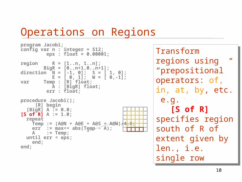
[S of R] A := 1.0;repeat Temp := (A@N + A@E + A@S + A@W)/4.0; err := max<< abs(Temp - A); A := Temp;until err < eps;
end;end;
Transform regions using “prepositional” operators: of, in, at, by, etc. e.g. [S of R]specifies region south of R of extent given by len., i.e. single row
Transform regions using “prepositional” operators: of, in, at, by, etc. e.g. [S of R]specifies region south of R of extent given by len., i.e. single row

11
Referencing 4 Nearest Neighborsprogram Jacobi;config var n : integer = 512; eps : float = 0.00001;
region R = [1..n, 1..n]; BigR = [0..n+1,0..n+1];direction N = [-1, 0]; S = [ 1, 0]; E = [ 0, 1]; W = [ 0,-1];var Temp : [R] float; A : [BigR] float; err : float;
procedure Jacobi(); [R] begin[BigR] A := 0.0;
[S of R] A := 1.0;repeat Temp := (A@N + A@E + A@S + A@W)/4.0; err := max<< abs(Temp - A); A := Temp;until err < eps;
end;end;
@d shifts applicable region in d direction
@d shifts applicable region in d direction
:= ( + + + )/4.0;
12
The “High Level” Logic Of J-Iterationprogram Jacobi;config var n : integer = 512; eps : float = 0.00001;
region R = [1..n, 1..n]; BigR = [0..n+1,0..n+1];direction N = [-1, 0]; S = [ 1, 0]; E = [ 0, 1]; W = [ 0,-1];var Temp : [R] float; A : [BigR] float; err : float;
procedure Jacobi(); [R] begin[BigR] A := 0.0;
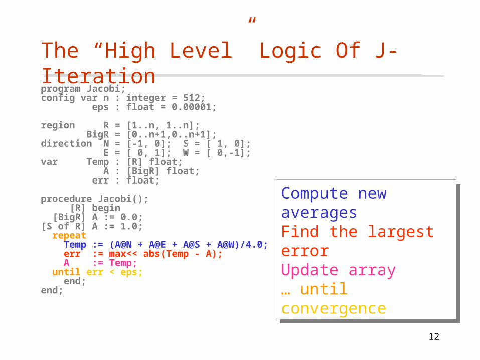
[S of R] A := 1.0;repeat Temp := (A@N + A@E + A@S + A@W)/4.0; err := max<< abs(Temp - A); A := Temp;until err < eps;
end;end;
Compute new averagesFind the largest errorUpdate array… until convergence
Compute new averagesFind the largest errorUpdate array… until convergence

13
ZPL In Detail ...ZPL has the usual stuff
– Datatypes: boolean, float, double, quad, complex, signed and unsigned integers: byte, ubyte, integer, uinteger, char, …
– Operators: • Unary: +, -, !• Binary: +, -, *, /, ^, %, &, | • Relational: <, <=, =, !=, >=, >=• Bit Operations: bnot(), band(), bor(), bxor(), bsl(), bsr()• Assignments: :=, +=, -=, *=, /=, %=, &=, |=
– Control Structures: if-then-[elseif]-else, repeat-until, while-do, for-do, exit, return, continue, halt, begin-end

14
ZPL Detail (continued)
• White space ignored
• All statements are terminated by semicolon (;)
• Comments are-- to the end of the line
/* */ all text within pairs including newlines
• All variables must be declared using var• Names are case sensitive
• Programs begin with program <name>;
the procedure with <name> is the entry point
15
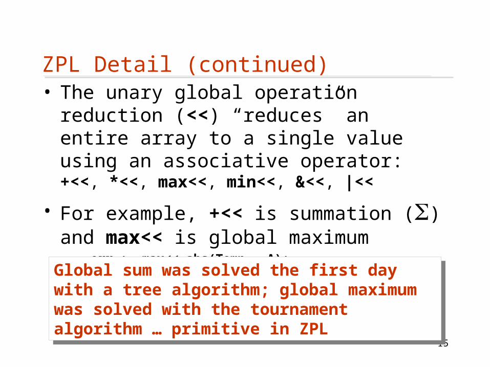
ZPL Detail (continued)• The unary global operation reduction (<<)
“reduces” an entire array to a single value using an associative operator: +<<, *<<, max<<, min<<, &<<, |<<
• For example, +<< is summation () and max<< is global maximum
err := max<< abs(Temp - A);
Global sum was solved the first day with a tree algorithm; global maximum was solved with the tournament algorithm … primitive in ZPL
Global sum was solved the first day with a tree algorithm; global maximum was solved with the tournament algorithm … primitive in ZPL
16
Bounding Box
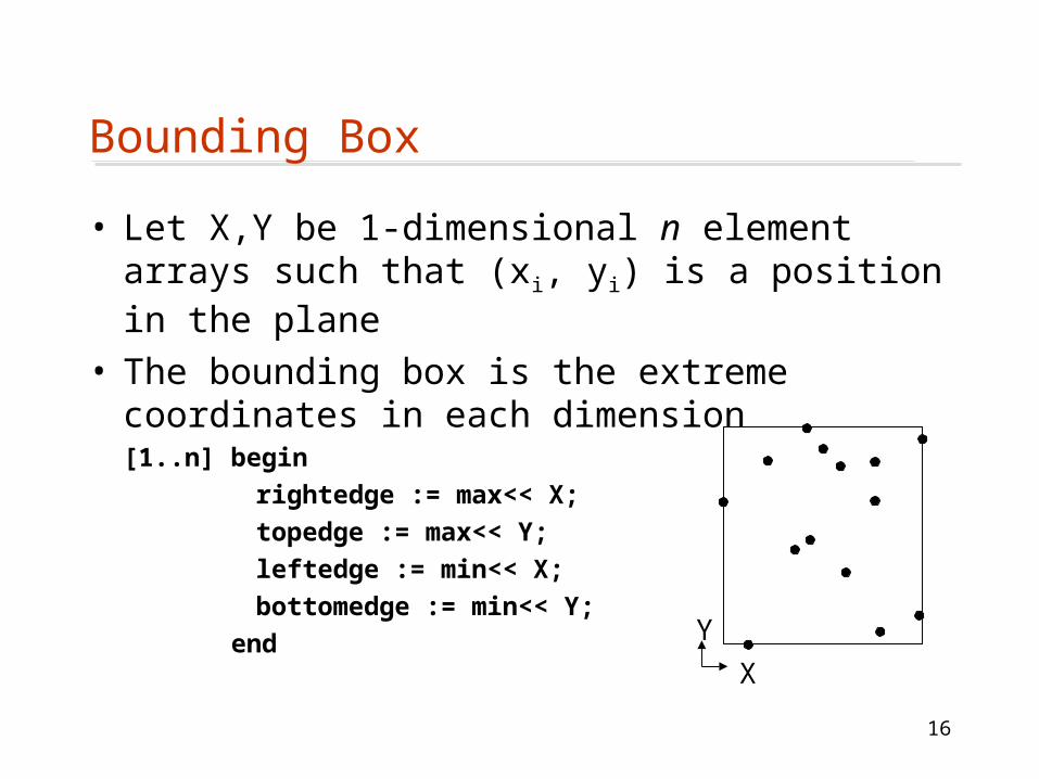
• Let X,Y be 1-dimensional n element arrays such that (xi, yi) is a position in the plane
• The bounding box is the extreme coordinates in each dimension[1..n] begin
rightedge := max<< X;
topedge := max<< Y;
leftedge := min<< X;
bottomedge := min<< Y;
endX
Y
17
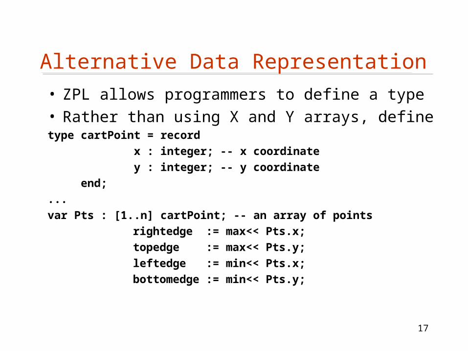
Alternative Data Representation
• ZPL allows programmers to define a type• Rather than using X and Y arrays, definetype cartPoint = record
x : integer; -- x coordinate
y : integer; -- y coordinate
end;
...
var Pts : [1..n] cartPoint; -- an array of points
rightedge := max<< Pts.x;
topedge := max<< Pts.y;
leftedge := min<< Pts.x;
bottomedge := min<< Pts.y;
18
ZPL Inherits from C
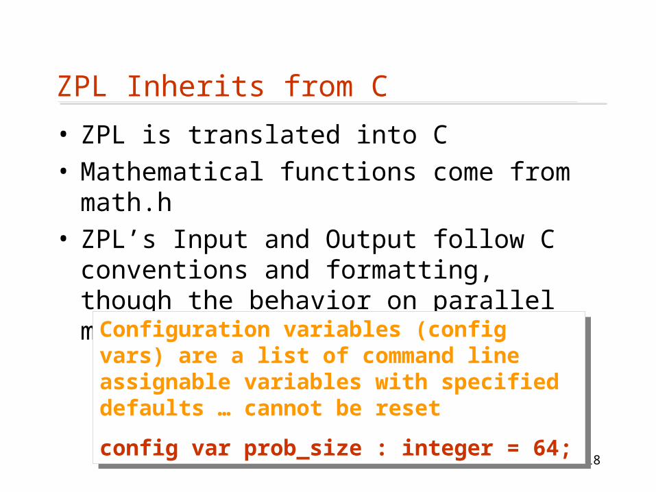
• ZPL is translated into C• Mathematical functions come from math.h• ZPL’s Input and Output follow C conventions
and formatting, though the behavior on parallel machines can differ
Configuration variables (config vars) are a list of command line assignable variables with specified defaults … cannot be reset
config var prob_size : integer = 64;
Configuration variables (config vars) are a list of command line assignable variables with specified defaults … cannot be reset
config var prob_size : integer = 64;
19
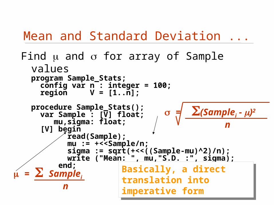
Mean and Standard Deviation ...
Find and for array of Sample valuesprogram Sample_Stats; config var n : integer = 100; region V = [1..n];
procedure Sample_Stats(); var Sample : [V] float; mu,sigma: float; [V] begin read(Sample); mu := +<<Sample/n; sigma := sqrt(+<<((Sample-mu)^2)/n); write ("Mean: ", mu,"S.D. :", sigma); end;
= Samplei
n
= (Samplei - )2
n
Basically, a direct translation into imperative form
Basically, a direct translation into imperative form

20
Regions
• Regions are named sets of index tuples• Regions are declared with syntax
region <name> = [<ll>..<ul> {, <ll>..<ul>}* ]
• For example region R = [1..n, 1..n]; -- Std 2-dim region
region V = [0..m-1]; -- 0-origin
• Short names common; caps by convention• Specify stride with by following the limits,
region Evens = [0..n by 2]; -- 0, 2, 4, ...
21
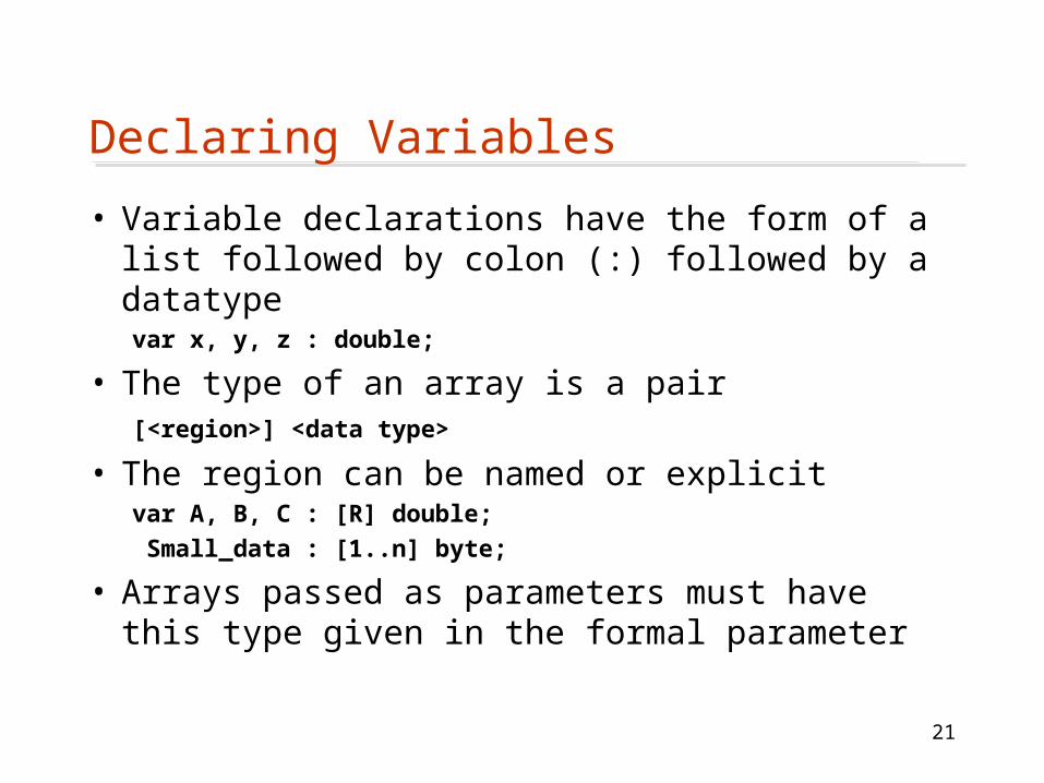
Declaring Variables
• Variable declarations have the form of a list followed by colon (:) followed by a datatypevar x, y, z : double;
• The type of an array is a pair [<region>] <data type>
• The region can be named or explicitvar A, B, C : [R] double;
Small_data : [1..n] byte;
• Arrays passed as parameters must have this type given in the formal parameter

22
Regions Controlling Array Stmt Execution
Regions specify the indices over which computation will be performed
• Specify region in brackets as statement prefix[1..n,1..n] A := B;
• The n2 elements of the region are replaced in A by their corresponding elements in B
• Regions are scoped[1..n,1] begin -- Work on first column only
A := 0;
B := 2*C;
end;

23
More About Regions
• With explicit indices leave a dimension blank to inherit from enclosing scope[1..n, 1] begin
X := Y; -- replace first column
[ , 2] X += X; -- double second column
end;
• Arrays must “conform” in rank and both define elements for indices of region
• “Applicable region” for assignments are (generally) the most tightly enclosing region of the rank of the left hand side
24
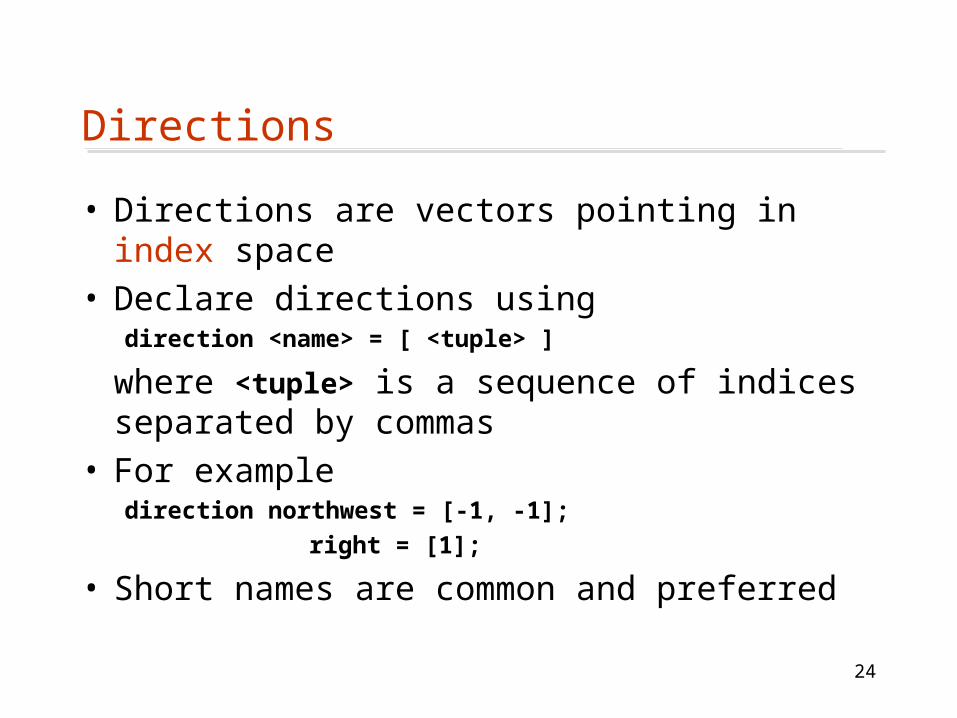
Directions
• Directions are vectors pointing in index space• Declare directions using
direction <name> = [ <tuple> ]
where <tuple> is a sequence of indices separated by commas
• For exampledirection northwest = [-1, -1];
right = [1];
• Short names are common and preferred

25
The @ Operator
The @ operator takes as operands an array variable and a direction, and returns an array whose values come from the given array offset from the prevailing region by direction[1..n,1..n-1] A := B@e; -- assume e = [0,1]
• Assign A[r,s] the value B[r,s+1]• That is, B@e contains the last n-1 columns of B, which are assigned to the first n-1 columns of A
:=The @ must reference defined values
The @ must reference defined values
26
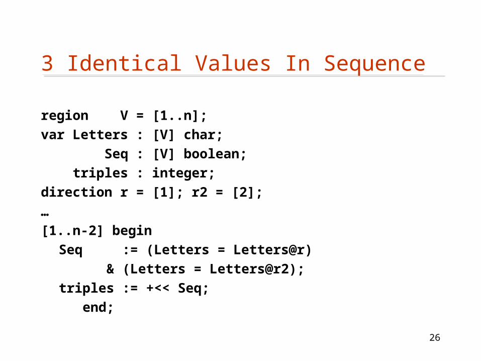
3 Identical Values In Sequence
region V = [1..n];
var Letters : [V] char;
Seq : [V] boolean;
triples : integer;
direction r = [1]; r2 = [2];
…
[1..n-2] begin
Seq := (Letters = Letters@r)
& (Letters = Letters@r2);
triples := +<< Seq;
end;

27
What Happens
abcd00000
P0
ddcb00000
P1
abcd00000
P2
eeeh00000
P3• Send left• Compare +1• Compare +2• Local +• Accum Tree• Bdcast Tree
abcddd00012
P0
ddcbab00002
P1
abcdee00002
P2
eeeh10002
P3

28
Region OperatorsZPL has region operators taking as operands a
region and a direction, and producing a region• at translates the region’s index set in the direction• of defines a new region adjacent to the given region along
direction edge and of direction extent
region R = [1..8,1..8]; C = [2..7,2..7];var X, Y : [R] byte;
region R = [1..8,1..8]; C = [2..7,2..7];var X, Y : [R] byte;
Direction e = [ 0,1]; n = [-1,0]; ne = [-1,1];
Direction e = [ 0,1]; n = [-1,0]; ne = [-1,1];
[C] X:= [C] X:= [C at e] Y:= [C at e] Y:= [n of C] Y:= [n of C] Y:= [C] Y:=X@ne [C] Y:=X@ne

29
Index1 ...
• ZPL comes with “constant arrays” of any size• Indexi means indices of the ith dimension
[1..n,1..n] begin
Z := Index1; -- fill with first index
P := Index2; -- fill with second index
L := Z=P; -- define identity array
end;
• These array -- of arbitrary dimension -- are compiler created using no space

30
Scan• Scan is the parallel prefix operation for
associative operators: +, *, min, max, &, |
• Scan is like reduction, but uses ||
• Prefix sum from the first lecture is +|| A 2 4 6 8 0
+||A 2 6 12 20 20
• Yes, “or scan” is ||| as in B 0 0 0 1 1 0 1 1
Run:=|||B 0 0 0 1 1 1 1 1
[2..n] Run := (Run != Run@w)*Index1;
pos := max<< Run;
Think globabllyThink globablly

31
Break
32
Recall Cannon’s Algorithmc11 c12 c13 a11 a12 a13 a14
c21 c22 c23 a21 a22 a23 a24
c31 c32 c33 a31 a32 a33 a34
c41 c42 c43 a41 a42 a43 a44
b13
b12 b23
b11 b22 b33
b21 b32 b43
b31 b42
b41
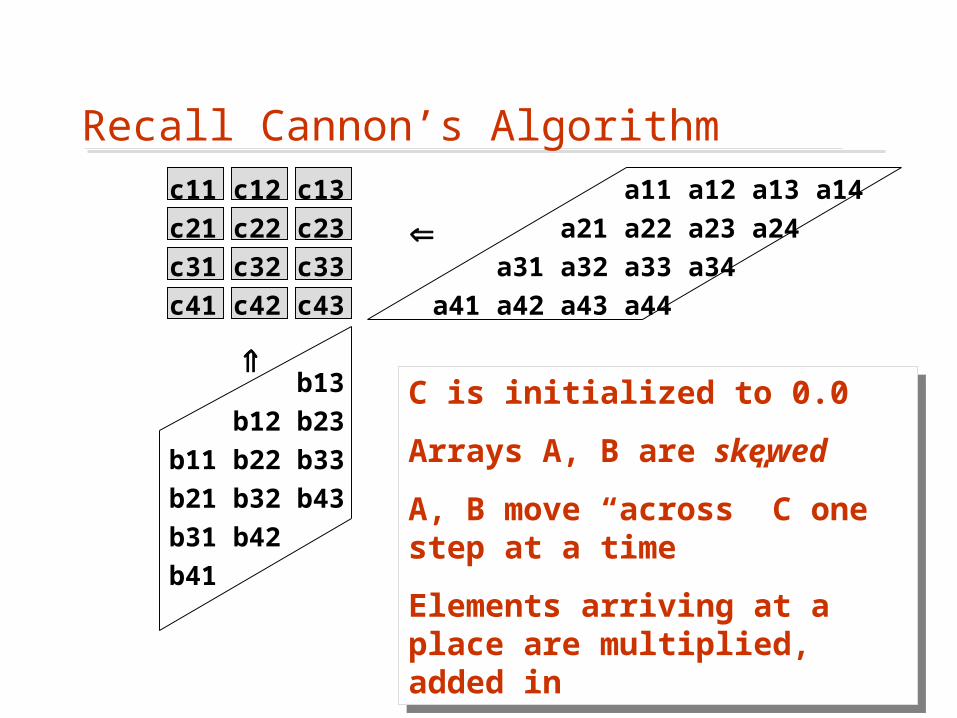
C is initialized to 0.0
Arrays A, B are skewed
A, B move “across” C one step at a time
Elements arriving at a place are multiplied, added in
C is initialized to 0.0
Arrays A, B are skewed
A, B move “across” C one step at a time
Elements arriving at a place are multiplied, added in

33
Programming Cannon’s In ZPL• Step 1: Handle the skewed arrays
c11 c12 c13 a11 a12 a13 a14
c21 c22 c23 a21 a22 a23 a24
c31 c32 c33 a31 a32 a33 a34
c41 c42 c43 a41 a42 a43 a44
b13 c11 c12 c13 a11 a12 a13 a14
b12 b23 c21 c22 c23 a22 a23 a24 a21
b11 b22 b33 c31 c32 c33 a33 a34 a31 a32
b21 b32 b43 c41 c42 c43 a44 a41 a42 a43
b31 b42 b11 b22 b33
b41 b21 b32 b43
b31 b42 b13
b41 b12 b23
Pack skewed arrays into dense arrays by rotation; process all n2 elements at once
Pack skewed arrays into dense arrays by rotation; process all n2 elements at once

34
Wrap-@
The @-operator has (recently) been extended to automatically wrap-around an array rather than “falling off” -- excellent for “periodic boundaries”:
var A : [1..n,1..n] double; -- array of doubles
…
A := A@^east; -- rotate columns left
:=
“Falling off” relative to the declared dimensions
“Falling off” relative to the declared dimensions
35
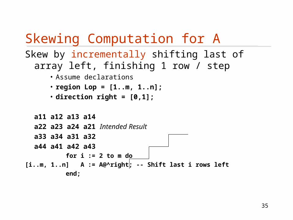
Skewing Computation for ASkew by incrementally shifting last of array left, finishing
1 row / step• Assume declarations• region Lop = [1..m, 1..n];• direction right = [0,1];
a11 a12 a13 a14
a22 a23 a24 a21 Intended Result
a33 a34 a31 a32
a44 a41 a42 a43 for i := 2 to m do
[i..m, 1..n] A := A@^right; -- Shift last i rows left
end;

36
Four Steps of Skewing A for i := 2 to m do
[i..m, 1..n] A := A@^right; -- Shift last m-i rows left
end;
a11 a12 a13 a14 a11 a12 a13 a14
a21 a22 a23 a24 a22 a23 a24 a21
a31 a32 a33 a34 a32 a33 a34 a31
a41 a42 a43 a44 a42 a43 a44 a41
Initial i = 2 step
a11 a12 a13 a14 a11 a12 a13 a14
a22 a23 a24 a21 a22 a23 a24 a21
a33 a34 a31 a32 a33 a34 a31 a32
a43 a44 a41 a42 a44 a41 a42 a43
i = 3 step i = 4 step
Skew B verticallySkew B vertically

37
Cannon’s Declarations
For completeness, when A is mn and B is np, the declarations are …
region Lop = [1..m, 1..n];
Rop = [1..n, 1..p];
Res = [1..m, 1..p];
direction right = [ 0, 1];
below = [ 1, 0];
var A : [Lop] double;
B : [Rop] double;
C : [Res] double;
38
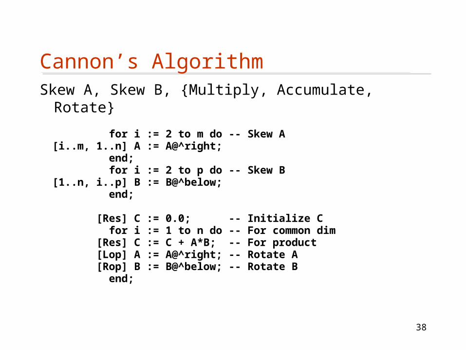
Cannon’s AlgorithmSkew A, Skew B, {Multiply, Accumulate, Rotate}
for i := 2 to m do -- Skew A [i..m, 1..n] A := A@^right; end; for i := 2 to p do -- Skew B [1..n, i..p] B := B@^below; end;
[Res] C := 0.0; -- Initialize C for i := 1 to n do -- For common dim [Res] C := C + A*B; -- For product [Lop] A := A@^right; -- Rotate A [Rop] B := B@^below; -- Rotate B end;

39
Combining Arrays of Different Ranks
An apparent limitation of ZPL (so far) is: Only arrays of like rank can be combined– Element-wise operators combine corresponding
elements: [R] A := B+C;– Sometimes combining arrays of different rank is
needed. E.g. Scale the elements of each row by the row maximum
• Find the row maximum: 2 dimension reduced to 1 dimension
• Divide each element of the row by its row max: 1 dimension applied to 2 dimensions
Two casesTwo cases

40
Don’t Change Rank
• Rather than change rank, use “singleton” values to collapse dimensions for lower rank
• For a region R = [1..m, 1..n], the rank 2 arrays R1 = [1..m, 1] and R2 = [1, 1..n] are regions corresponding to the first column and row
• ZPL is designed to exploit the similarity between an array with collapsed dimensions and a corresponding array of lower rank

41
The Reduction Case• Partial reduction applies reduction to an array
to produce a subarray … two regions needed• “Statement region” specifies the shape of the result• “Expression region” specifies the shape of the operand• The subarray that is combined is the subarray of the
operand formed by the singleton dimensions
[1..m,1] Max1 := max<< [1..m,1..n] A;
Statement region
Statement region
Max1 declared [1..m, 1]
Max1 declared [1..m, 1]
Partial reduction
Partial reduction
Expression region
Expression region
A declared [1..m, 1..n]
A declared [1..m, 1..n]

42
Partial Reduction (continued)
• All associative operators can be used in partial form: +, *, max, min, &, |
• The “singleton” dimension is “meaningful” in that the values are stored with like indices
• E.g. [1..m,1] is stored with other first column values
• Arrays can have arbitrary dimension values if they have the right rank & elements defined…
• E.g. Add row elements 2..n and store sum in 1st position• [1..m,1] A := +<< [1..m, 2..n] A;
+
43
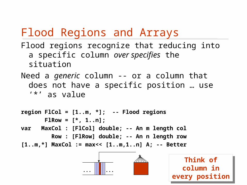
Flood Regions and ArraysFlood regions recognize that reducing into a
specific column over specifies the situation
Need a generic column -- or a column that does not have a specific position … use ‘*’ as value
region FlCol = [1..m, *]; -- Flood regions
FlRow = [*, 1..n];
var MaxCol : [FlCol] double; -- An m length col
Row : [FlRow] double; -- An n length row
[1..m,*] MaxCol := max<< [1..m,1..n] A; -- Better
+
......
Think of column in every position
Think of column in every position
44
Flood (continued)
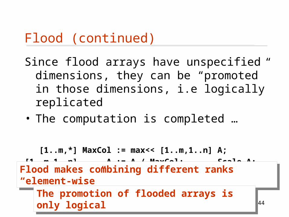
Since flood arrays have unspecified dimensions, they can be “promoted” in those dimensions, i.e logically replicated
• The computation is completed …
[1..m,*] MaxCol := max<< [1..m,1..n] A;
[1..m,1..n] A := A / MaxCol; --Scale A;
Flood makes combining different ranks “element-wise”Flood makes combining different ranks “element-wise”
The promotion of flooded arrays is only logicalThe promotion of flooded arrays is only logical
45
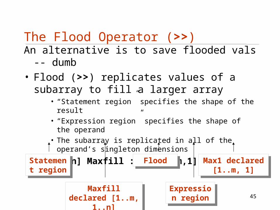
The Flood Operator (>>)An alternative is to save flooded vals -- dumb• Flood (>>) replicates values of a subarray to
fill a larger array• “Statement region” specifies the shape of the result• “Expression region” specifies the shape of the operand• The subarray is replicated in all of the operand’s
singleton dimensions
[1..m,1..n] Maxfill := >>[1..m,1] Max1;
Statement region
Statement region
Maxfill declared [1..m, 1..n]
Maxfill declared [1..m, 1..n]
FloodFlood
Expression region
Expression region
Max1 declared [1..m, 1]
Max1 declared [1..m, 1]
46
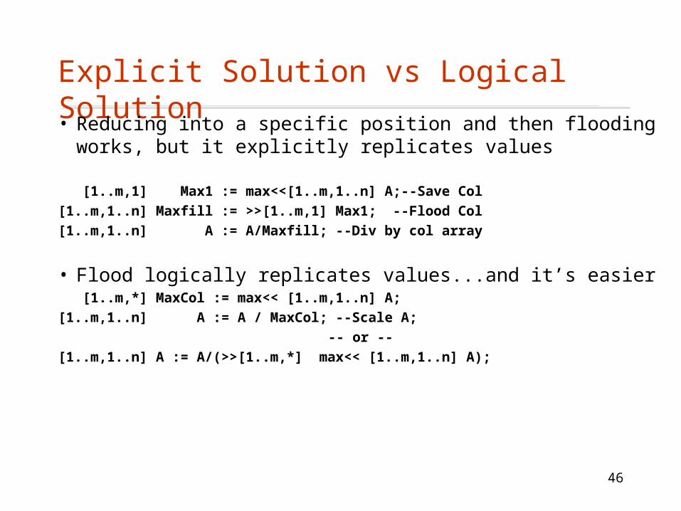
Explicit Solution vs Logical Solution • Reducing into a specific position and then flooding
works, but it explicitly replicates values
[1..m,1] Max1 := max<<[1..m,1..n] A;--Save Col
[1..m,1..n] Maxfill := >>[1..m,1] Max1; --Flood Col
[1..m,1..n] A := A/Maxfill; --Div by col array
• Flood logically replicates values...and it’s easier [1..m,*] MaxCol := max<< [1..m,1..n] A;
[1..m,1..n] A := A / MaxCol; --Scale A;
-- or --
[1..m,1..n] A := A/(>>[1..m,*] max<< [1..m,1..n] A);

47
Partial Scan• Partial scan would seen to be an easy
generalization of partial reduce, but since it doesn’t “collapse” dimensions, it is not necessary to specify a region, only a dimension
A := Index1;
B := +||[2] A;
A:1 1 12 2 23 3 3
B:1 2 32 4 63 6 9

48
Remembering Reduce, Scan & Flood
• The operators for reduce, scan and flood are suggestive …
• Reduce << produces a result of smaller size
• Scan || produces a result of the same size
• Flood >> produces a result of greater size
49
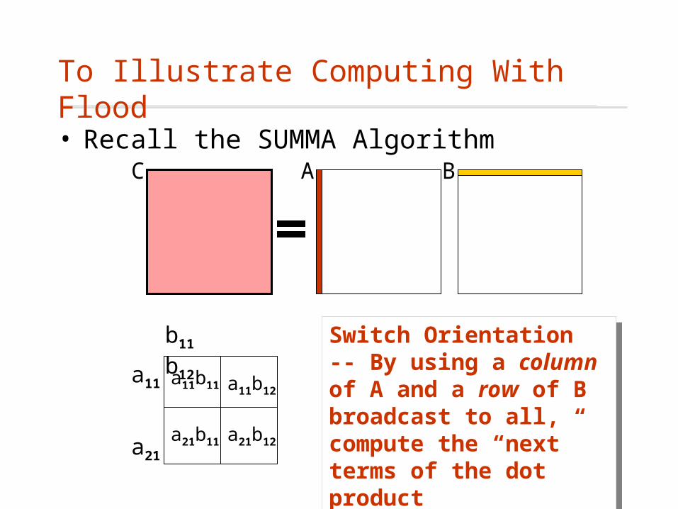
To Illustrate Computing With Flood
• Recall the SUMMA AlgorithmA BC
b11 b12
a11
a21
a11b11
a21b11
a11b12
a21b12
Switch Orientation -- By using a column of A and a row of B broadcast to all, compute the “next” terms of the dot product
Switch Orientation -- By using a column of A and a row of B broadcast to all, compute the “next” terms of the dot product
50
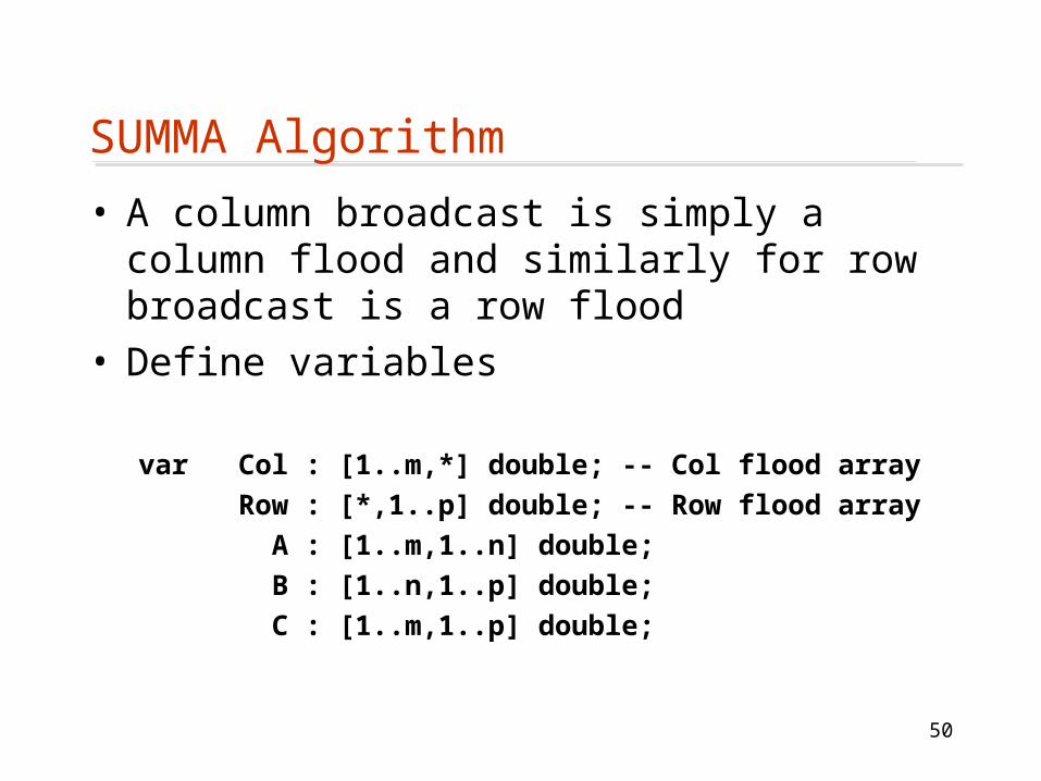
SUMMA Algorithm
• A column broadcast is simply a column flood and similarly for row broadcast is a row flood
• Define variables
var Col : [1..m,*] double; -- Col flood array
Row : [*,1..p] double; -- Row flood array
A : [1..m,1..n] double;
B : [1..n,1..p] double;
C : [1..m,1..p] double;
51
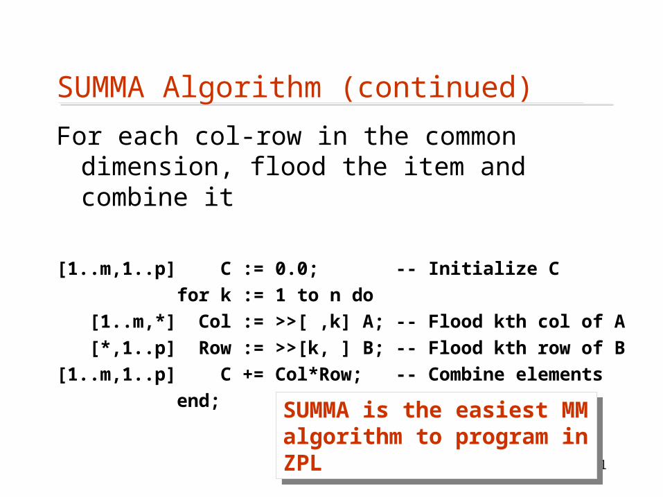
SUMMA Algorithm (continued)
For each col-row in the common dimension, flood the item and combine it
[1..m,1..p] C := 0.0; -- Initialize C
for k := 1 to n do
[1..m,*] Col := >>[ ,k] A; -- Flood kth col of A
[*,1..p] Row := >>[k, ] B; -- Flood kth row of B
[1..m,1..p] C += Col*Row; -- Combine elements
end;
SUMMA is the easiest MM algorithm to program in ZPL
SUMMA is the easiest MM algorithm to program in ZPL

52
SUMMA, The First Stepc11 c12 c13 a11 a12 a13 a14
c21 c22 c23 a21 a22 a23 a24
c31 c32 c33 a31 a32 a33 a34
c41 c42 c43 a41 a42 a43 a44
b11 b12 b13
b21 b22 b23
b31 b32 b33
b41 b42 b43
a11 a11 a11a21 a21 a21a31 a31 a31a41 a41 a41
b11 b12 b13b11 b12 b13b11 b12 b13b11 b12 b13
a11b11 a11b12 a11b13a21b11 a21b12 a21b13a31b11 a31b12 a31b13a41b11 a41b12 a41b13
Col Row
C

53
Cannon’s or SUMMA?
Which algorithm is better for MM?• Cannon’s algorithm uses the simpler
concepts and simpler operations• SUMMA is conceptually cleaner, but requires
ideas like flood arrays• We will analyze the two algorithms when we
have a performance model defined
54
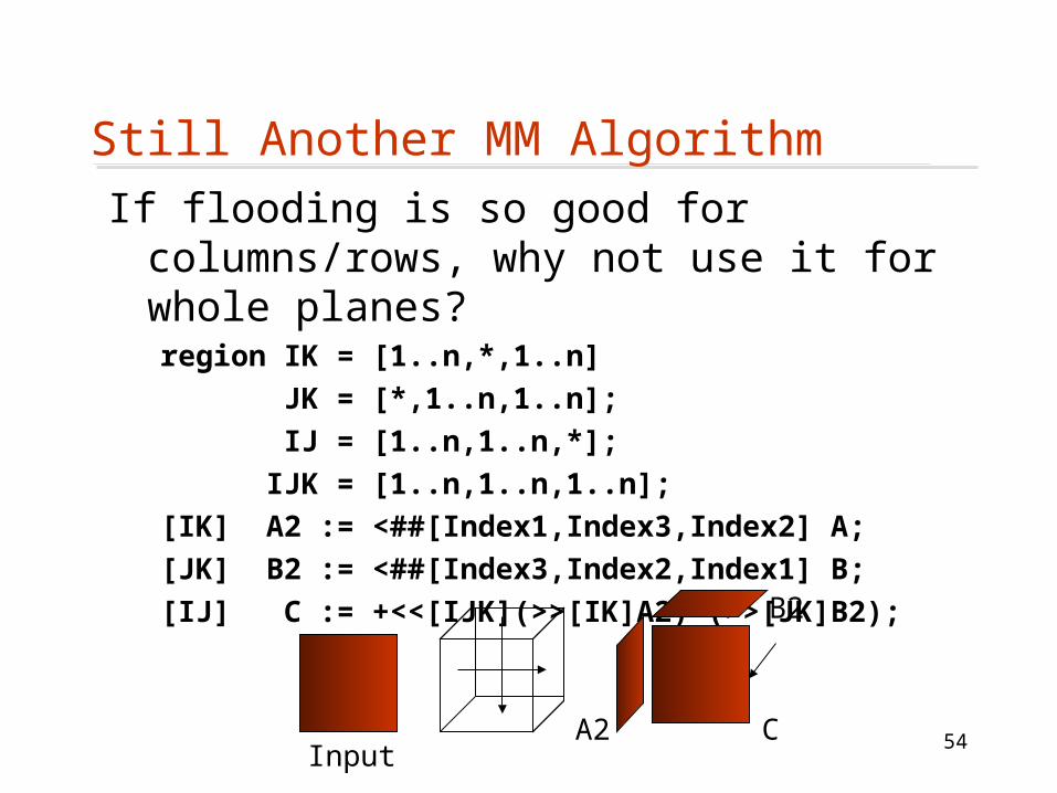
Still Another MM Algorithm
If flooding is so good for columns/rows, why not use it for whole planes?region IK = [1..n,*,1..n]
JK = [*,1..n,1..n];
IJ = [1..n,1..n,*];
IJK = [1..n,1..n,1..n];
[IK] A2 := <##[Index1,Index3,Index2] A;
[JK] B2 := <##[Index3,Index2,Index1] B;
[IJ] C := +<<[IJK](>>[IK]A2)*(>>[JK]B2);
InputA2
B2
C

55
ZPL Procedures• Procedures have form:
procedure <name> ({<params>}) {:Type};
<statement>;
• Parameters are listed with their type separated by commas:
procedure F(A, B : [R] byte, x : float): float;
• Values are returned with return … ;• Parameters are “called by value” as the default, but
by prefixing with var they can be called by referenceprocedure G(var A : [R] integer, big : integer);

56
A Procedure for Matrix Multiplicationprocedure MM (n: integer,
var A:[1..m,1..n] double,
var B:[1..n,1..p] double,
var C:[1..m,1..p] double);
var i : integer;
[1..m,1..p] begin
for k := 1 to n do
C += (>>[ ,k] A)*(>>[k, ]B);
end;
end;
MM(n, E, F, G); Explicit values in the parameter list force specific global variables to be used
Explicit values in the parameter list force specific global variables to be used

57
Rank Defined Formal ParametersIt is sufficient for the compiler to know the ranks of the
arrays, not their specific dimensional values … rank-defined parameters
• Use commas to imply the rank (r-1)• Call the procedure in the context of the proper region
procedure MM(n:integer, var A,B,C :[ , ] double);
var i : integer;
begin
for k := 1 to n do
C += (>>[ ,k] A)*(>>[k, ]B);
end;
end;
Inherit regions … call is
[1..m,1..p] MM(n,E,F,G);
Inherit regions … call is
[1..m,1..p] MM(n,E,F,G);

58
Promoting Scalar Procedures
• Procedures that only use scalar parameters, operations, etc. can be promoted to arrays
• Cannot use regions, array operations or other array-based notation
procedure sign (x: double) : integer;
if x < 0 then return -1
elseif x = 0 then return 0
else return 1;
[1..m, 1..n] A := sign(B);
Importing scalar computations from C is an application
Importing scalar computations from C is an application
59
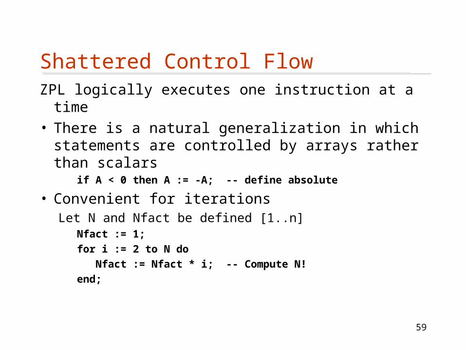
Shattered Control FlowZPL logically executes one instruction at a time
• There is a natural generalization in which statements are controlled by arrays rather than scalars
if A < 0 then A := -A; -- define absolute
• Convenient for iterationsLet N and Nfact be defined [1..n]
Nfact := 1;
for i := 2 to N do
Nfact := Nfact * i; -- Compute N!
end;
60
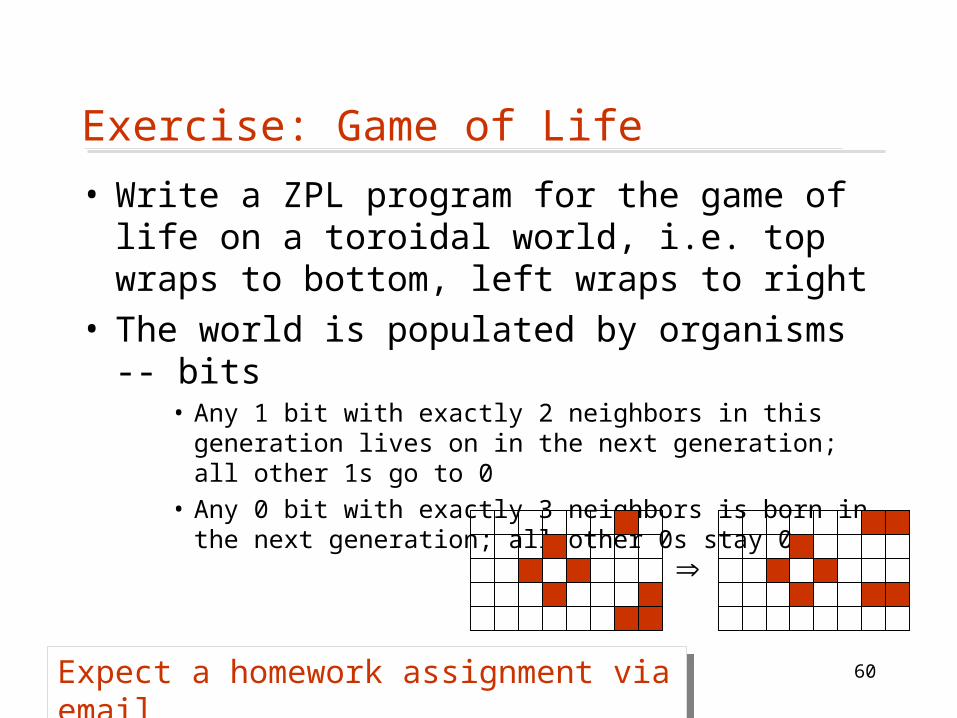
Exercise: Game of Life
• Write a ZPL program for the game of life on a toroidal world, i.e. top wraps to bottom, left wraps to right
• The world is populated by organisms -- bits• Any 1 bit with exactly 2 neighbors in this generation lives
on in the next generation; all other 1s go to 0• Any 0 bit with exactly 3 neighbors is born in the next
generation; all other 0s stay 0
Expect a homework assignment via emailExpect a homework assignment via email
61
Summary
• ZPL is an array programming language• Array programming emphasizes large
operations in which the compiler specifies the looping and indexing
• One new idea is the region -- set of indices• Programming in ZPL emphasizes thinking
about the task at a high level rather than at the detailed scalar level
![Presentation RAI Kwisthout.ppt [Compatibiliteitsmodus] · A novel view on computing • Traditional (Von Neumann) model of computation • Physically separated memory and computation](https://cdn.vdocuments.us/doc/165x107/5f6680c7a0299924ff2a5ae9/presentation-rai-compatibiliteitsmodus-a-novel-view-on-computing-a-traditional.jpg)


