Download - © 2014 Yuelu Duan - IDEALS

© 2014 Yuelu Duan
TECHNIQUES FOR LOW OVERHEAD FENCES AND SEQUENTIAL CONSISTENCYVIOLATION RECORDING
BY
YUELU DUAN
DISSERTATION
Submitted in partial fulfillment of the requirementsfor the degree of Doctor of Philosophy in Computer Science
in the Graduate College of theUniversity of Illinois at Urbana-Champaign, 2014
Urbana, Illinois
Doctoral Committee:
Professor Josep Torrellas, Chair and Director of ResearchProfessor Marc SnirProfessor Darko MarinovProfessor Yuanyuan Zhou, UC San DiegoDr. Pablo Montesinos, Qualcomm

Abstract
Fences are instructions that programmers or compilers insert in the code to prevent the compiler or the
hardware from reordering memory accesses [20, 43]. Fences can be expensive because all of the accesses
before the fence have to be finished (i.e., the loads have to be retired and the writes drained from the write
buffer) before any access after the fence can be observed by any other processor.
This thesis seeks to reduce the fence overhead in relaxed-consistency machines. It first introduces the
WeeFence, a fence that is very cheap because it allows post-fence accesses to skip it. Such accesses can
typically complete and retire before the pre-fence writes have drained from the write buffer. Only when an
incorrect reordering of accesses is about to happen, does the hardware stall to prevent it.
WeeFence presents implementation difficulties due to its reliance on global state and structures. This
thesis then introduces the Unbalanced Fence, which can optimize both the performance and the imple-
mentability of fences. Unbalanced Fence starts off with a design like WeeFence but without the global state,
which is called Weak Fence. Since the concurrent execution of multiple Weak Fences induces deadlock, a
Weak Fence is combined with the use of a conventional fence (i.e., Strong Fence) for the less performance-
critical threads. The result is called Unbalanced fence groups. Unbalanced fences are substantially easier
to implement than WeeFence, yet deliver comparable or higher performance.
For programs without sufficient fences, Sequential Consistency Violations (SCV) can occur and cause
programs to malfunction and are hard to debug. While there are proposals for detecting and recording SCVs,
they are limited in that they end program execution after detecting the first SCV because the program is now
non-SC. Therefore, they cannot be used in production runs. In addition, such proposals rely on expensive
hardware.
To address this problem, this thesis introduces the SCtame, an architecture for SCV detection and record-
ing that operates non-stop. SCtame re-uses part of the techniques of WeeFence and Unbalanced Fence to
detect SCVs. SCtame operates continuously because, after SCV detection and logging, it recovers and re-
ii
sumes execution while retaining SC. Hence, it can be used in production runs. In addition, SCtame is precise
in that it identifies only true SCVs — rather than dependence cycles due to false sharing. Finally, SCtame’s
hardware is not too costly because it is mostly local to each processor, and uses known recovery techniques.
iii

To my beloved wife, Yun, and my cute angel, Yiya.
To my mother and my father.
To my elder sister and younger brother.
iv

Acknowledgements
Many people helped and supported me throughout my Ph.D. research and made this journey much easier
and happier. I would like to express my earnest gratitude to all of them.
I want to first thank my advisor, Professor Josep Torrellas, who supported my research for five years
and continuously guided me and shared his experience. He was always willing to discuss on any topic that
I was exploring, and kept asking critical questions and polishing the ideas. He then worked hard together
with me and pushed it for perfection. I have learned many from him.
I also want to thank Wonsun Ahn, Abdullah Muzahid, and Nima Honarmand, whom I have worked
closely with. Wonsun helped on my first project in my Ph.D. years and continued the collaboration for
several times after that. He has been very encouraging, willing to help, and was often very insightful.
Abdullah worked together with me on the WeeFence project. Nima collaborated on the Unbalanced Memory
Fence project and made significant contributions.
I would also like to thank my fellow IACOMA-ers that I have overlapped with – Ulya, Xuehai, Shanxi-
ang, Adi, Wooil, Tom, Mengjia, Jiho, Yasser, Tanmay, Bhargava, and Raghavendra. They gave very useful
feedback in my group talks.
I want to thank my committee members, Professor Marc Snir, Professor Darko Marinov, Professor
Yuanyuan Zhou and Dr. Pablo Montesinos. They provided critical and insightful suggestions that made my
work much better than it was.
Thanks to Sherry for her help in everywhere – scanning and sending notes while I was remotely working,
taking care of the exam schedules, planning conference travels and many more. Thanks to the people in the
Academic Office – Kathy, Mary and others – for their endless and professional support since the first day.
Finally I want to mention my teachers, from elementary school to college, who established my per-
sonality and knowledge, and built my path that finally lead to Ph.D. research: Xuemei Yang, Aihong Qiu,
Meishui Zhan, Longbiao Wang, Xiaoguo Duan, Yujuan Jiang, Zhiqing Xie, Yinong Zheng, Wenjun Zhu,
v

Binyu Zang and Xiaobing Feng. I am honored to be one of their students. I want to thank Mr. Xianyou Xu,
who opened the door of computer programming to me and advised me in many ways ever since then.
vi

Table of Contents
List of Tables . . . . . . . . . . . . . . . . . . . . . . . . . . . . . . . . . . . . . . . . . . . . . . . ix
List of Figures . . . . . . . . . . . . . . . . . . . . . . . . . . . . . . . . . . . . . . . . . . . . . . x
Chapter 1 Introduction . . . . . . . . . . . . . . . . . . . . . . . . . . . . . . . . . . . . . . . . 11.1 Fence Overhead . . . . . . . . . . . . . . . . . . . . . . . . . . . . . . . . . . . . . . . . . 11.2 SC Violation Recording . . . . . . . . . . . . . . . . . . . . . . . . . . . . . . . . . . . . . 21.3 Thesis Contributions . . . . . . . . . . . . . . . . . . . . . . . . . . . . . . . . . . . . . . 4
Chapter 2 Background . . . . . . . . . . . . . . . . . . . . . . . . . . . . . . . . . . . . . . . . 62.1 Definitions . . . . . . . . . . . . . . . . . . . . . . . . . . . . . . . . . . . . . . . . . . . . 62.2 Sequential Consistency Violations . . . . . . . . . . . . . . . . . . . . . . . . . . . . . . . 72.3 Fences . . . . . . . . . . . . . . . . . . . . . . . . . . . . . . . . . . . . . . . . . . . . . . 82.4 Detecting SCVs . . . . . . . . . . . . . . . . . . . . . . . . . . . . . . . . . . . . . . . . . 8
Chapter 3 WeeFence: Toward Making Fences Free in TSO . . . . . . . . . . . . . . . . . . . . 103.1 Introduction . . . . . . . . . . . . . . . . . . . . . . . . . . . . . . . . . . . . . . . . . . . 103.2 WFence Design . . . . . . . . . . . . . . . . . . . . . . . . . . . . . . . . . . . . . . . . . 10
3.2.1 Skipping Fences & Avoiding SC Violations . . . . . . . . . . . . . . . . . . . . . . 103.2.2 Initial Design . . . . . . . . . . . . . . . . . . . . . . . . . . . . . . . . . . . . . . 123.2.3 Complete Design . . . . . . . . . . . . . . . . . . . . . . . . . . . . . . . . . . . . 133.2.4 Properties of the WFence Design . . . . . . . . . . . . . . . . . . . . . . . . . . . 15
3.3 Hardware Implementation . . . . . . . . . . . . . . . . . . . . . . . . . . . . . . . . . . . 153.3.1 Distributed Global Reorder Table (GRT) . . . . . . . . . . . . . . . . . . . . . . . . 17
3.4 Experimental Results . . . . . . . . . . . . . . . . . . . . . . . . . . . . . . . . . . . . . . 18
Chapter 4 Unbalanced Memory Fences: Optimizing Both Performance and Implementability . 214.1 Introduction . . . . . . . . . . . . . . . . . . . . . . . . . . . . . . . . . . . . . . . . . . . 214.2 Unbalanced Fences Design . . . . . . . . . . . . . . . . . . . . . . . . . . . . . . . . . . . 21
4.2.1 Main Idea . . . . . . . . . . . . . . . . . . . . . . . . . . . . . . . . . . . . . . . . 214.2.2 Strong Fence and Weak Fence . . . . . . . . . . . . . . . . . . . . . . . . . . . . . 234.2.3 A Taxonomy of Unbalanced Fence Groups . . . . . . . . . . . . . . . . . . . . . . 25
4.3 Examples of Unbalanced Fence Uses . . . . . . . . . . . . . . . . . . . . . . . . . . . . . . 294.3.1 Runtime Schedulers with Work Stealing . . . . . . . . . . . . . . . . . . . . . . . . 294.3.2 Software Transactional Memory . . . . . . . . . . . . . . . . . . . . . . . . . . . . 304.3.3 Bakery Algorithm . . . . . . . . . . . . . . . . . . . . . . . . . . . . . . . . . . . 304.3.4 Other Algorithms and Domains . . . . . . . . . . . . . . . . . . . . . . . . . . . . 31
vii

4.4 Discussion . . . . . . . . . . . . . . . . . . . . . . . . . . . . . . . . . . . . . . . . . . . . 324.5 Experimental Results . . . . . . . . . . . . . . . . . . . . . . . . . . . . . . . . . . . . . . 32
4.5.1 Experiment Setup . . . . . . . . . . . . . . . . . . . . . . . . . . . . . . . . . . . . 324.5.2 Performance Comparison . . . . . . . . . . . . . . . . . . . . . . . . . . . . . . . . 344.5.3 Performance Characterization . . . . . . . . . . . . . . . . . . . . . . . . . . . . . 384.5.4 Scalability Analysis . . . . . . . . . . . . . . . . . . . . . . . . . . . . . . . . . . 40
Chapter 5 Continuous and Precise Recording of Sequential Consistency Violations . . . . . . . 415.1 Introduction . . . . . . . . . . . . . . . . . . . . . . . . . . . . . . . . . . . . . . . . . . . 415.2 SCtame Design . . . . . . . . . . . . . . . . . . . . . . . . . . . . . . . . . . . . . . . . . 42
5.2.1 Continuous & Precise SCV Detection . . . . . . . . . . . . . . . . . . . . . . . . . 425.2.2 Reordered Accesses and SCVs . . . . . . . . . . . . . . . . . . . . . . . . . . . . . 425.2.3 Basic SCtame Operation . . . . . . . . . . . . . . . . . . . . . . . . . . . . . . . . 435.2.4 Types of Stalls . . . . . . . . . . . . . . . . . . . . . . . . . . . . . . . . . . . . . 455.2.5 Detecting a Deadlock . . . . . . . . . . . . . . . . . . . . . . . . . . . . . . . . . . 465.2.6 Recording the SCV . . . . . . . . . . . . . . . . . . . . . . . . . . . . . . . . . . . 485.2.7 Recovery from SCVs while Retaining SC . . . . . . . . . . . . . . . . . . . . . . . 49
5.3 Hardware Implementation . . . . . . . . . . . . . . . . . . . . . . . . . . . . . . . . . . . 505.3.1 RS Implementation and Operation . . . . . . . . . . . . . . . . . . . . . . . . . . . 505.3.2 The DDA Algorithm . . . . . . . . . . . . . . . . . . . . . . . . . . . . . . . . . . 525.3.3 HB Operation and Recovery . . . . . . . . . . . . . . . . . . . . . . . . . . . . . . 535.3.4 Hardware Complexity . . . . . . . . . . . . . . . . . . . . . . . . . . . . . . . . . 54
5.4 Experimental Results . . . . . . . . . . . . . . . . . . . . . . . . . . . . . . . . . . . . . . 555.4.1 Experiment Setup . . . . . . . . . . . . . . . . . . . . . . . . . . . . . . . . . . . . 555.4.2 SCV Detection . . . . . . . . . . . . . . . . . . . . . . . . . . . . . . . . . . . . . 575.4.3 SCtame Execution Time Overhead . . . . . . . . . . . . . . . . . . . . . . . . . . . 595.4.4 SCtame Characterization . . . . . . . . . . . . . . . . . . . . . . . . . . . . . . . . 605.4.5 SCtame Scalability Analysis . . . . . . . . . . . . . . . . . . . . . . . . . . . . . . 61
Chapter 6 Related Work . . . . . . . . . . . . . . . . . . . . . . . . . . . . . . . . . . . . . . . 636.1 Reducing Fence Overhead . . . . . . . . . . . . . . . . . . . . . . . . . . . . . . . . . . . 636.2 SCV Detection in Hardware . . . . . . . . . . . . . . . . . . . . . . . . . . . . . . . . . . 64
Chapter 7 Conclusions . . . . . . . . . . . . . . . . . . . . . . . . . . . . . . . . . . . . . . . . . 66
References . . . . . . . . . . . . . . . . . . . . . . . . . . . . . . . . . . . . . . . . . . . . . . . . 67
viii

List of Tables
4.1 A taxonomy of Unbalanced fence groups. . . . . . . . . . . . . . . . . . . . . . . . . . . . 254.2 Multicore architecture modeled. RT means round trip from the processor. . . . . . . . . . . 334.3 Applications used in the evaluation. . . . . . . . . . . . . . . . . . . . . . . . . . . . . . . 334.4 Characterization of Unbalanced fences under TSO. . . . . . . . . . . . . . . . . . . . . . . 35
5.1 Relationship between deadlocks and SCVs in SCtame. . . . . . . . . . . . . . . . . . . . . 455.2 Architecture modeled. RT stands for round trip. . . . . . . . . . . . . . . . . . . . . . . . . 555.3 Kernels that implement concurrency algorithms. . . . . . . . . . . . . . . . . . . . . . . . . 565.4 SCV detection for the kernel programs. . . . . . . . . . . . . . . . . . . . . . . . . . . . . 565.5 Number of runs to find all SCVs in RC. . . . . . . . . . . . . . . . . . . . . . . . . . . . . 585.6 Characterization of SCtame on RC. . . . . . . . . . . . . . . . . . . . . . . . . . . . . . . . 62
ix

List of Figures
1.1 Example of an SC violation. . . . . . . . . . . . . . . . . . . . . . . . . . . . . . . . . . . 31.2 Pattern for SC violation. . . . . . . . . . . . . . . . . . . . . . . . . . . . . . . . . . . . . 4
3.1 Averting an SC violation in a 2-WFence case. . . . . . . . . . . . . . . . . . . . . . . . . . 113.2 Averting an SC violation in a single-WFence case. . . . . . . . . . . . . . . . . . . . . . . . 113.3 Multicore augmented with WFence hardware. . . . . . . . . . . . . . . . . . . . . . . . . . 143.4 Interaction with WFence hardware structures. . . . . . . . . . . . . . . . . . . . . . . . . . 173.5 Performance impact on kernels for centralized GRT. In the figure, B and W refer to the
Baseline and WFence multicores. . . . . . . . . . . . . . . . . . . . . . . . . . . . . . . . . 193.6 Execution overhead of conservatively guaranteeing SC for centralized GRT. B and W mean
Baseline and WFence chips. . . . . . . . . . . . . . . . . . . . . . . . . . . . . . . . . . . 20
4.1 Eliminating global state without suffering from deadlock. . . . . . . . . . . . . . . . . . . . 224.2 Examples of using Unbalanced fences. . . . . . . . . . . . . . . . . . . . . . . . . . . . . . 244.3 Fence examples from work stealing (a) and STM (b). . . . . . . . . . . . . . . . . . . . . . 294.4 Using Unbalanced fences for the Bakery algorithm. . . . . . . . . . . . . . . . . . . . . . . 314.5 Execution time of CilkApps under TSO. . . . . . . . . . . . . . . . . . . . . . . . . . . . . 354.6 Execution time of CilkApps under RC. . . . . . . . . . . . . . . . . . . . . . . . . . . . . . 364.7 Transactional throughput of uSTM under TSO. . . . . . . . . . . . . . . . . . . . . . . . . . 374.8 Per-transaction breakdown of processor cycles. . . . . . . . . . . . . . . . . . . . . . . . . 384.9 Execution time of STAMP under TSO. . . . . . . . . . . . . . . . . . . . . . . . . . . . . . 394.10 Scalability of the reduction in fence stall time by WS+, W+, and Wee under TSO. . . . . . . 40
5.1 Example of a pattern that can create an SCV. . . . . . . . . . . . . . . . . . . . . . . . . . . 435.2 Examples of deadlocks caused by SCVs. . . . . . . . . . . . . . . . . . . . . . . . . . . . . 455.3 Other cases of deadlocks. . . . . . . . . . . . . . . . . . . . . . . . . . . . . . . . . . . . . 465.4 Example of deadlock detection and analysis. . . . . . . . . . . . . . . . . . . . . . . . . . . 485.5 The DDA algorithm, as executed by Pi. . . . . . . . . . . . . . . . . . . . . . . . . . . . . 525.6 RS size. . . . . . . . . . . . . . . . . . . . . . . . . . . . . . . . . . . . . . . . . . . . . . 595.7 Write buffer size. . . . . . . . . . . . . . . . . . . . . . . . . . . . . . . . . . . . . . . . . 595.8 Execution time of apps with IF-CoV (I) and SCtame (S) on RC. The bars are normalized to
plain hardware. . . . . . . . . . . . . . . . . . . . . . . . . . . . . . . . . . . . . . . . . . 605.9 Execution time of kernels with IF-CoV (I) and SCtame (S) on RC. The bars are normalized
to IF-CoV. . . . . . . . . . . . . . . . . . . . . . . . . . . . . . . . . . . . . . . . . . . . . 615.10 Scalability of SCtame. . . . . . . . . . . . . . . . . . . . . . . . . . . . . . . . . . . . . . 62
x

Chapter 1
Introduction
1.1 Fence Overhead
Fences are instructions that programmers or compilers insert in the code to prevent the compiler or the
hardware from reordering memory accesses [20, 43]. While there are different flavors of fences, the basic
idea is that all of the accesses before the fence have to be finished (i.e., the loads have to be retired and
the writes drained from the write buffer) before any access after the fence can be observed by any other
processor. The goal is to prevent a reordering that could lead to an incorrect execution.
Fences are used for low-overhead concurrency coordination in places where conventional synchroniza-
tion primitives such as locks would have too much overhead. In some cases, programmers insert explicit
fences in algorithms with fine-grain sharing. For instance, this is the case in the Cilk THE [15] work-stealing
algorithm. In the fast path of the algorithm, there are fences between two consecutive accesses to a queue
(e.g., to queue→head and queue→tail, respectively) that, if reordered by the compiler or hardware, could
cause incorrect execution.
In other cases, compilers insert fences. For example, in C++, the programmer can employ intentional
data races for performance, and declare the relevant variables as atomic [6] (or volatile for Java). Such
declaration prompts the compiler to insert a fence after the access and abstain from generating reordered
code; the fence then prevents the hardware from reordering accesses dynamically.
Fences can be expensive in current machines. A simple test on a desktop with an 8-threaded Intel Xeon
E5530 processor reveals that a fence introduces a significant visible overhead. If the write buffer is empty,
the fence introduces about 20 cycles; if there are many pre-fence write misses, then it may take an order of
magnitude more cycles until all the writes drain from the write buffer.
If fences did not stall the pipeline and, instead, had a negligible performance cost, software could take
advantage in two ways. First, programmers could write faster fine-grained concurrent algorithms. Second,
1

it would be feasible for C++ (or Java) programs to guarantee SC execution at little performance cost. To see
why, recall that a C++ compiler is required to generate SC code as long as any data race accesses are on vari-
ables declared as atomic. If fences could be skipped while retaining correctness, programmers could declare
all shared data as atomic, triggering the insertion of a fence after every single shared data access. However,
hardware reordering would not be curtailed. Moreover, while there would be a performance overhead due
to limiting compiler optimizations, recent work has indicated that such effect may be modest [30].
Current designs do not completely stall the pipeline on a fence while the write buffer drains. In-
stead, post-fence reads can speculatively load data. As long as no other processor observes the specula-
tive read, no problem can occur. If an external processor does (i.e., it initiates a coherence transaction on
the speculatively-read data), the local processor squashes the read and retries it. Unfortunately, even with
speculation, not all the fence stall is removed: speculative reads cannot retire until after the write buffer is
drained.
1.2 SC Violation Recording
Programmers writing and debugging multithreaded shared-memory programs assume the Sequential Con-
sistency (SC) memory model. Under SC, the memory operations of the program must appear to execute
in some global sequence as if the threads were multiplexed on a uniprocessor [24]. In practice, however,
current hardware overlaps, pipelines, and reorders memory accesses, unencumbered by programmer as-
sumptions. Unless the programmer uses correct synchronization to prevent certain reorders, an SC violation
(SCV) may occur, which is typically very hard to debug.
As an example, consider Figure 1.1(a). Processor P1 initializes variable a and then sets flag OK; later,
P2 tests the flag and, if set, uses a. If the hardware reorders the accesses as shown in arrows, where the
initialization of a is delayed, P2 ends up using an uninitialized variable. This order is an SCV.
An SCV occurs when a dependence cycle takes place [40]. For a two-threaded SCV, two conditions
need to be satisfied. First, we need to have two data races, where a race occurs when two threads access the
same memory location without an intervening synchronization and at least one is writing. In the example,
we have races on variables a and OK. Second, at runtime, these races must overlap in time and intertwine
in a manner that forms a cycle. For the example, this is shown in Figure 1.1(b). The dashed arrows show
program order, while the solid ones show the order of dependences: A2 executed before A3, while A4
2

P P1 2
A1: a=init
A2: OK=TRUE
(a)
P P
(b)
1 2
A1: wr a
A3: if (OK)
A3: rd OK
A4: rd aA2: wr OK
Data dependenceProgram order
A4: ...=a
Figure 1.1: Example of an SC violation.
executed before A1, effectively forming a cycle. A cycle can be formed with any number of threads.
An SCV is a type of concurrency bug that, while not as common as popular bugs like data races, is
important for three reasons. First, it can induce harm by causing a program to execute in a totally counter-
intuitive manner. Second, it is hard to debug, as it depends on the timing of events, and single-stepping
debuggers cannot reproduce it. Finally, it is typically concentrated in critical codes, such as those that
perform fine-grain communication and synchronization — synchronization libraries, task schedulers, and
run-time systems.
There are proposals of hardware schemes to detect and record SCVs [28, 29, 32, 33]. However, they
have limitations. Specifically, some schemes are very conservative, as they only look for a single data race
where the two participating accesses are more-or-less concurrent [28, 29].
The other schemes look for dependence cycles [32, 33]. However, they terminate execution after de-
tecting the first SCV. This is because the program state is now non-SC and, therefore, incorrect. Further
execution could find artificial, additional SCVs. This approach is incompatible with production runs and,
therefore, suboptimal, as some SCVs may only happen during production runs. Instead, we would like to
log the SCV bug for later debugging, and continue at production-run speeds under strict SC-enforced exe-
cution, in order to correctly capture future SCVs. A second limitation of these schemes is that they rely on
expensive hardware. Specifically, they modify the coherence protocol or introduce many hardware tables,
whose information needs to be passed between processors.
3

PA
(b)
PB
A1: t0 = y
A0: x = 1 B0: y = 1
B1: t1 = x
Program orderDependence
PA PB
A1: t0 = y
A0: x = 1 B0: y = 1
B1: t1 = x
(c)
PA
(a)
PB
A0: x = 1 B0: y = 1
A1: t0 = y B1: t1 = x
PA
t0 = t1 = x = y = 0
PB
A0: x = 1 B0: y = 1
A1: t0 = y B1: t1 = x
(d)
fencefence
Figure 1.2: Pattern for SC violation.
1.3 Thesis Contributions
This thesis seeks to 1) reduce the fence overhead and 2) record Sequential Consistency Violations more
efficiently. For the first problem, we observe that more aggressive reordering is acceptable as long as it
does not result in an incorrect access order. Specifically, it is fine for a remote processor to observe local
post-fence accesses before the local write buffer is drained, as long as no dependence cycle occurs — that
is, as long as no SC violation occurs [40].
We first introduce an aggressive fence design that we call WeeFence, or WFence for short. It allows
post-fence accesses to skip the fence and proceed without stalling. Such accesses can typically complete
and retire before the pre-fence writes drain from the write buffer. This is beyond today’s most aggres-
sive speculative fence implementations, where speculative reads cannot retire until after the write buffer is
drained. Hence, WFence can save substantial time when write misses pile up before the fence. Only when
an incorrect reordering of accesses is about to happen, does WFence stall until such a event cannot occur; in
the large majority of cases, WFence induces zero visible stall. Finally, WFence is compatible with the use
of conventional fences in the same program.
WFence presents implementation difficulties due to its reliance on global state and structures. We then
introduce Unbalanced Fence that can optimize both the performance and the implementability of fences.
Unbalanced Fence starts off with a design like WeeFence but without the global state, which is called Weak
Fence. Since the concurrent execution of multiple Weak Fences induces deadlock, a Weak Fence is combined
with the use of a conventional fence (i.e., Strong Fence) for the less performance-critical threads. The result
is called Unbalanced fence groups. Unbalanced fences are substantially easier to implement than WeeFence,
yet deliver comparable or higher performance.
To address the limitations of current SC violations detection schemes, we introduce a new architecture
for SCV detection and logging called SCtame. SCtamecan continuously detect SCVs. In SCtame, when a
4

processor Pi executes an out-of-order access A, the hardware in Pi prevents other processors from seeing it
by rejecting coherence transactions received by Pi directed to the address accessed by A. Pi only responds
when all accesses prior to A complete. When an SCV between two or more processors happens, a deadlock
occurs. In this case, SCtame quickly detects the deadlock, records the SCV, and recovers and resumes
execution while maintaining SC. As a result, SCtame operates under SC continuously, and can be used in
production runs.
In addition, SCtame is precise and has a modest hardware cost. SCtame is precise in that it records
only true SCVs — rather than dependence cycles due to false sharing. SCtame’s hardware is not too costly
because it is mostly local to each processor, and uses known recovery techniques.
5

Chapter 2
Background
2.1 Definitions
For clarity, we start by defining the terms performed, retired, completed, and M-speculative (or speculative
relative to the memory consistency model), as we will use them to refer to different stages in the execution
of a load or store in an out-of-order processor. For a load instruction, we say that it performs when the data
loaded returns from the memory system and is deposited into a register. A load retires when it reaches the
head of the Reorder Buffer (ROB) and has already performed. After retirement, the load completes.
A store instruction retires when it reaches the head of the ROB and its address and data are available.
At this point, the store is deposited into the write buffer. If the write buffer was empty, the store is merged
with the memory system, potentially triggering a coherence transaction. When the coherence transaction
terminates (e.g., when all the invalidation acknowledgments have been received), we say that the store has
performed, and is now completed. At this point, the store is removed from the write buffer.
In some memory models, multiple stores in the write buffer can be merged with memory concurrently
and, therefore, perform (and complete) in any order. In other models, stores have to perform (and complete)
in program order. In this case, as a store is deposited in the write buffer, if there is an older store in it, it
waits until the older one completes and is removed from the buffer.
The memory consistency model supported by the hardware determines the access reorders that are legal
within a thread [3]. For example, in SC, every load and store must appear to perform in program order.
In Total Store Ordering (TSO) [2], loads can perform before older stores, but load-load reordering and
store-store reordering are not allowed. Consequently, only the store at the head of the write buffer can be
performing at any given time. In Release Consistency (RC) [18], loads can perform before older stores, and
both load-load and store-store reordering are allowed. As a result, multiple stores in the write buffer can be
performing at a given time.
6

In practice, hardware implementations allow loads to be performed earlier than allowed by the memory
model — as long as the load is not observed by other processors [17]. A local load is observed when the
processor receives a coherence transaction directed to the data read by the load. During the period between
when a load is performed and when it can be performed according to the memory model, we say that the
load is M-speculative (or speculative relative to the memory consistency model). We use this term to denote
that this status depends on the memory consistency model supported by the system. For example, consider
a load (l2) that performs while an earlier one in the pipeline (l1) is not yet performed. Under RC, l2 is not
M-speculative. However, under TSO, l2 is M-speculative until l1 performs.
While a load is M-speculative, if it is observed, the load and subsequent instructions are squashed.
When the load ceases to be M-speculative, it will not be squashed if it is observed (even if it is not retired).
Squashing is simple to do because the load state is all still buffered in the ROB structures.
2.2 Sequential Consistency Violations
In some cases, allowing memory reorderings (such as the TSO model) results in a violation of SC. This is
shown in Figure 1.2(a). Initially, variables t0, t1, x, and y are zero. Processor PA first writes 1 to x and then
reads y into t0, whereas processor PB first writes 1 to y and then reads x into t1. Under SC, either A1 or B1
is the last access in the global order of accesses. Hence, after the execution of the code, either t0 is 1, t1 is
1, or both are 1. However, under TSO, it may happen that, while the A0 write is waiting in the write buffer,
the A1 load reads the initial value of y and retires. Then, B0 and B1 execute. Finally, A0 completes. We then
have an effective order of A1, B0, B1, and A0. This causes both t0 and t1 to be zero, which is impossible
under SC. It is an SC Violation (SCV).
Shasha and Snir [40] show what causes an SCV: overlapping data races where the dependences end up
ordered in a cycle. Recall that a data race occurs when two threads access the same memory location without
an intervening synchronization and at least one is writing. Figure 1.2(b) shows the order of the dependences
at runtime that causes the cycle and, therefore, the SCV. In the figure, the source of the arrow is the access
that occurs first. If at least one of the dependences occurs in the opposite direction (e.g., Figure 1.2(c)), no
cycle (and therefore no SCV) occurs.
7

2.3 Fences
Given the pattern in Figure 1.2(a), Shasha and Snir [40] prevent the SCV by placing one fence between
references A0 and A1, and another between B0 and B1. The result is Figure 1.2(d). Now, as we run the
program in a TSO machine, A1 waits for A0 to complete, while B1 waits for B0. As a result, either A1 or
B1 is the last operation to complete, and there is no SCV.
In practice, programmers typically include explicit fences in performance-critical applications with
fine-grained sharing. Examples include run-time systems, schedulers, tasks managers, and soft real-time
systems. If fences were very cheap, programmers could improve the performance and scalability of these
codes.
Compilers insert fences in codes to prevent incorrect reorderings. In particular, in high-level languages
such as C++ or Java, the programmer is allowed to employ intentional data races for performance, as long
as the relevant variables are declared as atomic or volatile. Such declarations prompt the compiler to insert
a fence after the access, which prevents any reordering by the compiler or hardware. Without the fences,
some reorderings could be harmless, while others — like the one in Figure 1.2(b) — could cause SCVs.
2.4 Detecting SCVs
Recall that an SCV occurs when multiple threads participate in a cycle created by data dependences and
program orders. There are several hardware schemes that try to detect SCVs in a relaxed-consistency ma-
chine [28, 29, 32, 33]. They can be classified into conservative ones and highly-specific ones. The con-
servative schemes [28, 29] look for one necessary condition for an SCV, namely a data race where the two
participating accesses are more-or-less concurrent. However, this is very conservative because most races
are not accompanied by a second, cycle-forming data race.
The highly-specific schemes (i.e., Vulcan [32] and Volition [33]) leverage cache-coherence transactions
to dynamically track the data dependences between processors, looking for a cycle pattern like Figure 1.1(b).
While they are very effective at finding SCVs, they have two limitations.
The first one is that, after they find the first SCV in a program, they are unable to retain SC. The
program state is now non-SC and, therefore, incorrect. As a result, they terminate execution. Note that the
ability to retain SC and continue is crucial. It allows the machine to find further true SCVs in the execution
8

— as opposed to “fabricated” ones due to the execution already being non-SC. Hence, these schemes are
incompatible with production runs and, therefore, suboptimal, as some SCVs may only happen during
production runs.
The second limitation is that they rely on expensive hardware. They introduce elaborate hardware struc-
tures for metadata. In hardware, they time-stamp the dynamic accesses of individual processors, and then
compare the time-stamps on interprocessor communication. The time-stamps are passed through augmented
or special coherence transactions. Word-level dependence disambiguation is attained with additional per-
word state and especial transitions (Vulcan) or special hardware structures (Volition). Vulcan only detects
two-processor cycles on a snoopy protocol; Volition detects cycles with any number of processors in a scal-
able protocol, but requires elaborate hardware to record dependences between processors, combine them,
and pass them around. In this thesis, we use simpler, mostly-local hardware and rely on known recovery
mechanisms.
A related approach is to use hardware to only enforce SC (e.g., [5, 9, 17, 19, 27, 35, 45]). These schemes
look for a necessary condition for an SCV and, when detected, squash instructions to force the threads away
from the SCV path. In most schemes, the necessary condition is the presence of an access that is observed
while it is M-speculative relative to SC. For example, in Figure 1.1(b), the access is store A2.
Unfortunately, these schemes are not usable to detect SCVs. This is because, when they squash in-
structions to avoid the SCV, they discard the state that would be needed for SCV detection and recording.
In addition, in most cases, as we will see, we would have a false positive because no SCV would end up
happening. We describe these schemes in Section 6.
9

Chapter 3
WeeFence: Toward Making Fences Free inTSO
3.1 Introduction
Programmers and compilers insert fences in the code to prevent the compiler or the hardware from reorder-
ing memory accesses. The goal is to inexpensively manage the order in which the memory accesses of a
thread are observed by other threads.
If fences could be skipped while retaining correctness, programmers can declare all shared data as
atomic, and the compiler would would insert fences and then automatically guarantee SC at little perfor-
mance cost. The key is that hardware-induced reordering would not be curtailed. Moreover, while there
would be a performance cost due to limiting compiler optimization, recent work has indicated that such
effect may be modest [30].
Current processors speed-up fences with in-window load speculation [17]. With this technique, a post-
fence read can speculatively get the value from memory even while the fence is not completed — i.e., while
pre-fence writes are not completed or pre-fence reads are not retired. The post-fence read cannot retire, but
the processor uses its value while actively monitoring for any external coherence transaction on the cache
line read. If such a transaction is received, the processor squashes and re-executes (at least) the post-fence
read and its successors. The post-fence read can only retire after the fence completes. Hence, in many cases,
the pipeline can still get stalled because a post-fence read has to wait.
3.2 WFence Design
3.2.1 Skipping Fences & Avoiding SC Violations
WeeFence, or WFence for short, is a new fence design that typically executes without inducing visible
processor stall. It allows the memory instructions that follow the fence to proceed without stalling. While the
10

wr x(1)
rd y
PBPA
rd y
PBPA
xx
(1)
(2)
wr xWfence1
rd y rd xWfence2
wr y
PA PB
execute(2) Wfence1 Wfence2
wr y
rd x
PS
x
(a) (b)
Wfence1 Wfence2
wr ywr x
PSy
rd x
PS (3)
(4)
(c)
(5) local checkstall
Figure 3.1: Averting an SC violation in a 2-WFence case.
(2)
PB
wr x(1)
rd y
PA
PS
x
yBS
rd y
PBPA
x
yBS
(1)
(2)
wr xWfence1
rd y
wr y
PA PB
(a)
wr x
wr y
Wfence1execute
(b)
Wfence1
wr ywr x
PS
stall/retry
coherence
(4)
(c)
wr x wr x(3)
Figure 3.2: Averting an SC violation in a single-WFence case.
WFence idea can be used for different memory consistency models, in this thesis, we focus on a design for
TSO [43] because TSO is very similar to the model used by x86 processors [39]. In this case, post-WFence
read instructions can complete and retire before the WFence completes — i.e., before the pre-WFence writes
complete.
This is beyond today’s most aggressive speculative fence implementations, where post-fence read in-
structions can speculatively load data, but cannot retire until all of the pre-fence writes complete. As a
result, a WFence can save substantial time when write misses pile up before the fence. In the large majority
of cases, WFence induces no stall, as all of its actions are hidden by the ROB, and the instruction retiring
rate is unaffected by the presence of a fence. Moreover, WFence is compatible with the use of conventional
fences in the same program.
Since WFence enables aggressive memory access reordering, it needs to watch for incorrect reorders
that lead to SC violations. For example, if any of the two fences in Figure 1.2(d) allowed its post-fence
read to be ordered before its pre-fence write, an SC violation could occur. Hence, when WFence is about
to allow a reorder that can lead to an SC violation, it stalls for a short period of time until such a condition
cannot occur. This case, however, is rare.
11

WFence uses some extensions in the processor and memory system. They involve registering pending
pre-fence accesses in a table, which other processors can check against post-fence accesses to see if there is
a possibility for an SC violation. These actions reuse existing cache coherence protocol transactions.
3.2.2 Initial Design
Consider the basic pattern shown in Figure 1.2(d), where two fences are needed to avoid an SC violation.
In Figure 3.1(a), we repeat the example and use WFences, therefore enabling reordering. To prevent an SC
violation, WFence has to ensure that, if PA:rd y happened before PB:wr y (arrow (1)), then PB:rd x stalls
until it is ordered after PA:wr x — and hence, arrow (2) is forced to point downward and no SC violation
occurs.
A WFence involves two steps. First, the execution of a WFence instruction consists of collecting the
addresses to be written by the pending pre-WFence writes, encoding them in a signature, and storing the
signature in a table in the shared memory system called the Global Reorder Table (GRT). We call such
addresses the Pending Set (PS) of the WFence. The return message of such a transaction brings back from
the GRT to the processor the combined addresses in the PSs of all the currently-active WFences in other
processors — in a signature. The incoming signature is saved in a processor register called the Remote
Pending Set Register (RPSR).
In the second step, any post-WFence read compares its address against those in the RPSR. If there is
no match, the read executes and may go on to eventually retire even before the WFence completes — a
WFence completes when all pre-WFence accesses retire and complete, which requires that all pre-WFence
writes drain from the write buffer. If, instead, there is a match, the read stalls. The stall lasts until all the
remote WFences whose PSs are in the local RPSR complete. At that point, an arrow like (2) in Figure 3.1(a)
cannot occur. When a WFence completes, it clears its GRT entry. Moreover, it needs to remove its PS
addresses from any other processor’s RPSR. This last requirement makes this initial design suboptimal; it is
eliminated in Section 3.2.4.
The procedure described allows high concurrency by using conventional speculative execution. A post-
WFence read instruction can execute even before the WFence has executed (and filled the local RPSR with
the PS of all the other currently-active WFences). In this case, when the RPSR is finally filled, the read’s
address is compared to it, and the read is squashed if there is a match. The squashed read immediately
12

restarts and, if it still matches, stalls. Moreover, when a post-WFence read stalls due to a match, subsequent
local reads that do not match can still execute speculatively. However, because of the TSO model, they
can only retire after the stalled read retires. Finally, a speculative read (stalled or otherwise) is squashed
and restarted if it receives an external coherence access or if its line is evicted from the cache. Overall, the
key insight is that a post-WFence read instruction can stop being speculative and retire before the earlier
WFence completes; we will see when.
Figures 3.1(b) and (c) illustrate the algorithm. In Figure 3.1(b), WFence1 deposits its PS addresses in
the GRT (1) and, since the GRT is empty, returns no addresses. PA:rd y skips WFence1 (2) and executes
because PA’s RPSR is empty. Later, in Figure 3.1(c), WFence2 deposits its PS addresses in the GRT (3)
and returns the PS addresses of the active fences (4). At this point, an arrow like (1) in Figure 3.1(a) may
have happened; hence WFence has to prevent an arrow like (2) in Figure 3.1(a). Therefore, as shown in
Figure 3.1(c), as PB:rd x tries to skip WFence2, it checks the local RPSR (5) and finds a match. It then
stalls until WFence1 completes, removing the possibility of an arrow like (2) in Figure 3.1(a).
Stalling is rare, as it requires that two WFences dynamically overlap in time, that both threads access
the same addresses in opposite sides of the fences, and that both dependence arrows threaten to go upward.
3.2.3 Complete Design
In the case discussed, both threads had fences to prevent the reordering of their accesses. However, a
dependence cycle can occur even if only one of the threads reorders its accesses. Hence, in patterns where
only one thread has a WFence, SC violations can still occur. In the case of TSO, the pattern is shown in
Figure 3.2(a).
In Figure 3.2(a), assume that PA:rd y happened before PB:wr y (arrow (1)). TSO ensures that PB:wr x
is ordered after PB:wr y. However, a reorder of the accesses in PA (rd y ordered before wr x) could cause a
dependence cycle. Hence, WFence has to ensure that, if PA:rd y happened before PB:wr y (arrow (1)), then
PB:wr x stalls until PA:wr x has finished — preventing arrow (2).
This cycle cannot be avoided with the support described in Section 3.2.2. Since PB has no fence, PB:wr
x does not know of (and cannot wait on) any remote PS. Instead, we must stall the consumer of the first
arrow, namely PB:wr y. For this, we will leverage the coherence transaction triggered by PB:wr y, and stall
the transaction until no cycle can occur.
13

To do so, we extend the WFence operation of Section 3.2.2 with two additional steps. We call the
addresses read by the post-WFence read instructions executed before the WFence completes the Bypass Set
(BS). In the first step, as the post-WFence reads execute, they accumulate the BS addresses in a table in the
local cache controller. Such table is called the Bypass Set List (BSL).
Second, as external coherence transactions from other processors are received, their addresses are
checked against the BSL. If there is a match and the local read is still speculative, conventional specula-
tion automatically squashes the read and, therefore, we remove the read address from the BSL. However, if
there is a match and the local read is already retired (although the WFence is not complete), the incoming
transaction is not satisfied — it is either buffered or bounced. Later, when the local WFence completes,
the BSL is cleared, and any transaction waiting on a BSL entry is satisfied. It is only at this point that the
requesting access from the remote processor can complete. Any subsequent access in that processor can
then proceed, but it is too late to create a cycle with the local processor because all pre-WFence writes have
completed.
Figures 3.2(b) and (c) illustrate the algorithm for our example. In Figure 3.2(b), WFence1 deposits its
PS addresses in the GRT (1). As PA:rd y skips the fence and executes (2), it is part of the BS and hence
saves its address (3). Later, in Figure 3.2(c), as PB:wr y executes, it issues a coherence transaction to PA.
Assume that PA:rd y has already retired and, hence, an arrow like (1) in Figure 3.2(a) will be generated. As
the request arrives, it checks the BSL and matches. The request is either buffered or asked to retry. When
WFence1 completes, the BS addresses are deallocated and the coherence request is satisfied. At this point,
PB:wr y completes. After this, as PB:wr x completes, it cannot generate an arrow like (2) in Figure 3.2(a)
because PA:wr x has already completed.
ProcessorSet Register (RPSR)Remote Pending
Bypass Set List(BSL)
Network
L1 cache
RPSR: Signature with the union of all other processor’s PS addressesBSL: Unordered list of this processor’s BS addresses
− Signature of the PS addresses
Global Reorder Table (GRT)
PS signature
GRT: Shared table that has, for each processor that has an active WFence
Signature of evicted BS addresses
from cache− Signature of BS addresses whose dirty cache lines were evicted
Figure 3.3: Multicore augmented with WFence hardware.
14
3.2.4 Properties of the WFence Design
The WFence design resulting from the previous two sections has two key features. The first one is that when
a WFence completes, it does not need to notify any other processor; the second is that conventional fences
are seamlessly supported. We consider each in turn.
Recall from Section 3.2.2 that, when a WFence completed, in addition to clearing its GRT entry, it
would have to clear its PS addresses in other processors’ RPSRs. Now, thanks to the BSL, this is no longer
required. Now, when a WFence completes, it only needs to clear its GRT entry. The other processors
that contain the WFence’s PS addresses in their RPSR will continue to wait (on a match) only until their
own WFence completes. Once their own WFence completes, it can be shown that no dependence cycle is
possible anymore and, therefore, they can clear their RPSR. This has the major advantage that no remote
messages need to be sent, and the wait terminates on a local event.
To see why, consider Figure 3.1(c) again. WFence2 is the second WFence to reach the GRT and it
brings address x to its RPSR. PB:rd x must wait on the RPSR, but only until WFence2 completes. At this
time, PB can safely clear its RPSR and let rd x commit, since no arrow like (2) in Figure 3.1(a) is possible.
The reason is that: (i) if WFence2 is complete, then PB:wr y completed; (ii) PB:wr y completion required
that the BSL of PA had been cleared and, therefore, that WFence1 in PA had completed; (iii) finally, if
WFence1 had completed, then PA:wr x must have completed and an arrow like (2) is not possible. In all
cases, post-WFence reads waiting due to a match in the local RPSR to avoid a cycle can proceed as soon as
their local WFence completes. A WFence never clears RPSR entries in other processors.
The second feature is that conventional fences are seamlessly compatible with the use of WFences in
the same program. Indeed, a conventional fence affects a WFence as in the case described in Section 3.2.3:
one of the interacting threads cannot reorder its accesses, either because the memory model prevents it (like
in Section 3.2.3) or because there is a conventional fence.
3.3 Hardware Implementation
Figure 3.3 shows the three hardware structures needed to support WFences: RPSR, BSL, and GRT. The
RPSR is a register in the processor that contains a signature generated with a Bloom filter. It is filled when
the processor receives the response from the GRT to a WFence executed by the processor. The RPSR
15
contains the union of the (line) addresses in the Pending Sets (PSs) of all the WFences that were active (i.e.,
were in the GRT) at the time when the processor executed the WFence (and visited the GRT). The RPSR
is automatically cleared when the local WFence completes. There is also a functional unit that intersects
the addresses of the post-WFence reads issued by the processor against the RPSR, and stalls the reads that
match.
The BSL is a list of addresses in the cache controller. It stores the (line) addresses in the Bypass Set
(BS), namely the addresses read by post-WFence read instructions that are executed by the processor while
the WFence is incomplete. One such read instruction may be retired or still speculative. If the read is
speculative, it will be squashed (and removed from the BSL) in these four cases: (1) the response to the
WFence execution fills the RPSR with a signature that includes the read’s address, (2) the data loaded
by the read receives a coherence transaction or (3) is evicted from the cache, or (4) the read is in a mis-
speculated branch path. In all of these cases but the last one, the read is retried. The addresses of incoming
coherence transactions are checked against the BSL. If one matches a BSL address for a retired read, then
the coherence transaction is not allowed to complete — it is either stalled or bounced.
A dirty cache line that was accessed by a retired read in the BSL may be evicted from the cache. If we
evicted it without taking any special action, the processor would not observe future coherence activity on
the line. Consequently, when such a line is evicted, as it is written back to memory, its address is saved
in the GRT entry of the processor. Since coherence transactions always check the GRT, the GRT will be
able to stall (or bounce) future conflicting transactions on that address. To prevent overflow of these evicted
entries in the GRT, they are encoded in the GRT in a per-processor signature. While these signatures may
cause false-positive stalls, it can be shown that, if they use the same encoding as the RPSR, deadlocks are
impossible.
Note that if the evicted cache line accessed by a retired read in the BSL was clean, no action is needed.
Since the directory is not updated, the local processor will still observe future coherence activity on the line.
Overall, in all cases, the BSL (and the processor’s GRT entry) is cleared when the local WFence completes.
The Global Reorder Table (GRT) is a table in the memory system that is shared by all the processors. It
is placed in a module that observes coherence transactions, such as the directory controllers in a distributed-
directory system, or the bus controller in a snoopy-based system. It has at most one entry per processor.
When a processor sends a WFence-execution message with its PS addresses to the GRT, the hardware
16

creates an entry in the GRT. The entry contains the PS (line) addresses encoded in a signature. The entry is
active until the WFence completes. The GRT entry for a processor may also contain a signature with (line)
addresses from the WFence’s BS. It contains the addresses (also present in the BSL) of dirty lines that were
evicted from the cache due to a conflict.
Figure 3.4 shows how pre-WFence writes, WFence execution, post-WFence reads, and WFence com-
pletion interact with the hardware structures. For WFence execution and completion, we show the general
case where a GRT access is needed.
Else put address in the local BSL (if BSL is full, stall the read)
Clear the local BSL and release any external transactions waiting on it
Put signature of own PS addresses in GRT
addresses and store it in the local RPSR
1. Pre−WFence write:
3. Post−WFence read:
Clear the processor’s entry in the GRT
2. Local WFence execution (most general case):
4. Local WFence completion (most general case):
Return from GRT a signature of the union of other processors’ PS
Stall the request if it finds a matching address in the local RPSR
Stall the request if it finds the matching address in a remote BSL
Clear the local RPSR and release any local reads waiting on it
Figure 3.4: Interaction with WFence hardware structures.
3.3.1 Distributed Global Reorder Table (GRT)
For a small multicore, we use a centralized GRT associated with the bus controller. For a larger machine,
we propose a scalable design of a distributed GRT. The GRT is distributed like a directory, broken down into
modules in charge of address ranges. Each module is associated with the corresponding directory module.
With such a design, as we follow the algorithms for WFence execution and completion in Figure 3.4, we
see that a WFence may need to communicate with multiple GRT modules. Specifically, it needs to deposit a
signature in all of the modules that map any address in its Pending Set (PS); it needs to read a signature from
all of the modules that map any address that may be in its Bypass Set (BS). Unfortunately, such a distributed
protocol is prone to races when multiple processors concurrently communicate with sets of GRT modules.
Hence, we radically simplify the algorithm.
17

Our simplifications rely on several observations. First, data accesses tend to have spatial locality. In
addition, we assign address ranges to GRT modules at page-level granularity, and use a first-touch page
allocation policy. As a result, a WFence’s PS often maps to a single GRT module. Similarly, the WFence’s
BS will often map to the same GRT module as its PS. Furthermore, if there is no need for the WFence to
perform a GRT access (a common case), then it does not matter where the BS maps to. Finally, it is always
correct for a WFence to operate as a conventional fence.
With these insights, we design the WFence execution algorithm for the distributed GRT as follows. As
the WFence collects its PS addresses, it determines whether they all map to a single GRT module. If they
do, then the WFence executes as usual, communicating with the single GRT module. In this case, which is
the common one, there are no race concerns.
Otherwise, the WFence works as a conventional fence: the GRT is unused and post-fence reads remain
speculative until the fence completes. This approach ensures that there are no multiple WFences racing to
create multiple GRT entries with inconsistent state.
In all cases, post-WFence reads execute speculatively as usual, without any concern about the GRT
distribution. However, when a read is at the ROB head ready to retire after a fence that executed as a
WFence, it checks two conditions: (i) whether the WFence communicated with any GRT module and,
(ii) if so, whether the read maps to the same GRT module. The very common case is that either it did
not communicate with any module or, if it did, the module is the one where the read maps to, and the
read address is not in the RPSR. In this case, the read retires immediately as in our centralized WFence.
Otherwise, the read will not retire until the WFence completes — preventing the retirement of subsequent
accesses.
3.4 Experimental Results
For our evaluation, we perform detailed cycle-level execution-driven simulations using SESC [37]. We
compare two multicore architectures: one with WFences (WFence) and one with conventional fences that
support in-window load speculation and exclusive store prefetching [17] (Baseline). We run two sets of
programs. The first one is 6 programs that we obtain from [7, 8, 15] and use explicit fences for correctness.
We call these programs kernels. We study the performance that WFence attains over Baseline.
The second set is 17 C/C++ programs from SPLASH-2 and PARSEC, and pbzip2 (parallel bzip2). We
18

use LLVM to simply turn every access to potentially shared data into an atomic access. This prevents the
compiler from reordering across these accesses, inducing a measured execution overhead of about 4% on
average (which is consistent with [30]). In addition, as the compiler generates the binary code, it inserts a
fence after each atomic write, to prevent the hardware from reordering it with any subsequent read. We call
the transformed code SC-apps. In our evaluation, we study the performance overhead of these fences using
either WFence or Baseline.
Figure 3.5 compares the execution time of the kernels on the Baseline and WFence multicores with the
centralized GRT. Kernel execution times are normalized to those in Baseline, and broken down into time
stalled in fences (Fence) and the rest (Useful). The figure shows that, in Baseline, these kernels spend an
average of 12% of their time stalled in fences. WFence eliminates most of such stall, reducing the execution
time of the kernels by an average of 11%. This shows the effectiveness of our new fence.
bakery dekker lazylist ms2 peterson worksteal avg70
80
90
100
Nor
mal
ized
Exe
cutio
n T
ime
B B B B B B B
WW W
WW
W
W
Useful Fence
Figure 3.5: Performance impact on kernels for centralized GRT. In the figure, B and W refer to the Baselineand WFence multicores.
Figure 3.6 shows the execution time overhead induced in the applications by transforming them into
SC-apps, conservatively guaranteeing SC. The overheads come from limiting compiler-induced optimiza-
tion (Compiler) and reducing hardware-induced reordering (Fence). Compiler is largely the same in both
Baseline and WFence multicores, and adds, on average, 4% overhead. For some codes, limiting compiler
optimization slightly improves the speed (Compiler is negative), causing the bar to start lower than zero.
19

bar
nes
fm
m
oce
an
radio
sity
raytr
ace
water
-ns
water
-sp
chole
sky
fft
radix
blac
k
fluid
swap
tions
cann
eal
ded
up
stre
am
pbz
ip2 av
g-20
0
20
40
60
80
100
120
Exe
cutio
n O
verh
ead(
%)
B
B
B
B
B
B
B B
BB
B
B
B
B BB
B
B
W
W
WW
WW W
WW W
W W WW W
W
WW
Compiler Fence
Figure 3.6: Execution overhead of conservatively guaranteeing SC for centralized GRT. B and W meanBaseline and WFence chips.
20

Chapter 4
Unbalanced Memory Fences: OptimizingBoth Performance and Implementability
4.1 Introduction
The WeeFence [14] design, while effective, is challenging to implement in a distributed-directory environ-
ment. There are two reasons, which stem from the schemes’ reliance on updating and collecting global state.
First and foremost, it suffers from coherence protocol races. In general, a fence needs to collect Remote
PS state from different directory modules (since the state is distributed according to physical addresses).
Such state needs to be consistent. Unfortunately, multiple processors may be depositing Pending Set (PS)
and reading PS from multiple directory modules with some unknown interleaving. Obtaining a consistent
view is hard. We believe that this problem is still unsolved. To avoid this problem, if a WeeFence needs to
deposit/access PS to/from more than one directory module, we turn it into a conventional fence — which
hurts performance.
The second reason is that handling the global state adds complexity. It requires: adding new coherence
messages to get pending sets, augmenting protocol messages with address sets, adding the GRT hardware
table in the directory, and collecting addresses into signatures.
4.2 Unbalanced Fences Design
4.2.1 Main Idea
Our goal is to design a fence architecture that optimizes both performance and hardware implementability.
The insight is that, if we eliminate the global-state requirements of aggressive-design fences like WeeFence
or AAF, and use the resulting fence in combination with conventional fences, we have eliminated most of
the implementation challenges while retaining much of the performance. We call this approach Unbalanced
Fences. In the following, we describe the ideas in the context of WeeFence.
21

Minimizing Hardware Cost.
wr x
P1
BS
wr y
P2
rd xrd y
y
(b)
Conventional_FenceWeeFence_NoGRT1
wr x
P1
BS
wr y
P2
rd y
y
rd z
BS
rd x
z
wr z
P3
(c)
WeeFence_NoGRT1 WeeFence_NoGRT2 Conventional_Fence
wr x
P1
BS
wr y
P2
rd xrd y
y
(a)
WeeFence_NoGRT2WeeFence_NoGRT1
Figure 4.1: Eliminating global state without suffering from deadlock.
The reason why WeeFence needs to save state in the GRT global table is to avoid deadlock when prevent-
ing an SCV. If there was no such global state, at the onset of an SCV, the processors would deadlock. This
can be seen in Figure 4.1a, which is WeeFence without GRT or PS. In the figure, P1:rd y has completed,
while P1:wr x is still pending (and hence address y is in P1’s BS). Moreover, P2:wr y is still incomplete
and, as its request is issued into the network, it bounces off P1’s BS. WeeFence NoGRT2 would then be
bypassed, and P2:rd x would execute, placing address x in P2’s BS. The future execution of P1:wr x would
issue a transaction that would bounce off P2’s BS. The system would then enter deadlock.
In WeeFence, however, P1 deposits its PS (i.e., address x) in the GRT while bypassing WeeFence1, and
P2 reads the GRT when it finds WeeFence2. Then, P2:rd x is unable to execute because its address collides
with what was read from the GRT. Later, P1:wr x finishes, WeeFence1 completes, P1’s BS is cleared, and
P2:wr y can make progress.
Our insight is that, if at least one of the fences in the Fence Group is a conventional fence, there is no
need for the GRT or PS state. This is shown in Figure 4.1b for a 2-fence group, and in Figure 4.1c for a
3-fence group.
Consider Figure 4.1b first, where P2 now uses a conventional fence. The execution state is the same
as in Figure 4.1a: P1:rd y has completed, P1’s BS has address y, and P2:wr y is bouncing. However, the
conventional fence prevents P2:rd x from executing non-speculatively — i.e., if P2:rd x executes, it must
remain speculative, and a coherence message from P1:wr x will squash it. As a result, P1:wr x does not
stall and completes. This will complete WeeFence NoGRT1, clear P1’s BS, and enable P2:wr y to make
progress.
Similarly, in Figure 4.1c, where only P3 uses a conventional fence, there is no deadlock possible. In the
worst case, P2:wr y is stalled by P1’s BS and P3:wr z is stalled by P2’s BS. However, P3:rd x cannot stall
22

P1:wr x.
In summary, we have moved from an N-fence group with all WeeFences, to one where N-1 fences are
WeeFences without global state and one is a conventional fence. This simplifies the hardware implementa-
tion substantially.
Retaining High Performance.
In many cases, a program where individual fence groups contain both WeeFence NoGRTs and conventional
fences can deliver as much performance as if all the fence groups only included WeeFences. This is because,
in a fence group, there is often one or more threads that execute performance-critical operations, while the
other threads do not. Consequently, we use WeeFence NoGRTs in the former threads and conventional
fences in the latter. The result is that the overall program performance is the same as if all the threads used
WeeFences.
Ladan-Mozes et al. [22] observed that, in a two-fence group, there is sometimes a thread that is more
important than the other. In this thesis, we focus on fence groups with any number of threads.
Two examples where we can combine WeeFence NoGRT and conventional fences are algorithms in
work stealing and in software transactional memory (STM). Specifically, in the Cilk runtime system [15], a
thread accessing its task queue can conflict with a thread stealing a task. Both owner and thief use fences
to avoid an SCV. Since, typically, the owner accesses its deque much more frequently than a thief, we use a
WeeFence NoGRT in the owner code and a conventional fence in the thief code.
In STM, there are fences when threads read a variable, write a variable, and commit a transaction. In
the STM scheme that we use later, when a thread that reads a variable conflicts with another that writes the
same variable, their fences prevent an SCV. Since reads are more frequent and time-critical than writes, we
use a WeeFence NoGRT in the read code and a conventional fence in the write code.
4.2.2 Strong Fence and Weak Fence
Based on this discussion, we define an Unbalanced fence group as one that is composed of one or more
Strong Fences (sFs) and one or more Weak Fences (wFs). A sF is a conventional fence. It allows post-
fence loads to execute speculatively, but not to complete, before the fence completes. On a conflict with an
external coherence message, the load is squashed.
23

A wF is a WeeFence with no GRT or PS, augmented with a few small additions that we will describe.
It allows the same post-fence accesses as WeeFence to execute, retire, and complete before the fence com-
pletes. Specifically, under TSO, these are post-fence reads; under RC, they can be post-fence reads or writes.
The addresses accessed by post-fence accesses are placed in the BS. When one such access is complete, the
BS will reject incoming transactions that conflict with it.
Recall from WeeFence [14] that the BS is stored in a hardware list in the cache controller, and that it
can include a front-end Bloom-filter to reduce the number of comparisons.
The comparison between BS addresses and coherence transaction addresses has to be done at line gran-
ularity. This is because the coherence protocol, which is used to detect dependences, uses line addresses.
Figure 4.2a shows why using finer-grain addresses (e.g., word-level) would cause an incorrect result. The
example is like Figure 4.1b, except that P2 writes to word y’ before writing to y, where words y’ and y share
the same line. If the comparison between the BS and the coherence transaction (1) induced by P2:wr y’ was
done at word granularity, there would not be a match. Hence, the line would be brought to P2 and, later,
P2:wr y would complete execution locally, potentially causing an SCV.
wF
rd y
wF
wr x
rd y
wF
wr x
rd y
wF
P1 P1 P2
(1) wr y’wr y
rd x
wF
(c)BS y
P1 P2
(1) wr y’wr y
sF
rd x
(a)
(b)
P2
rd x
wr y’ wr x
Figure 4.2: Examples of using Unbalanced fences.
We expect Unbalanced fences to be used in codes that require high performance — possibly in li-
braries such as those for work-stealing scheduling, STM, or synchronization. These codes are typically
programmed by expert programmers. It is reasonable for these programmers, for example, to place a sF in
the code of the owner thread in a work-stealing runtime, and a wF in the code of the thief thread.
However, it is not reasonable for these programmers to know or worry about false sharing. Consequently,
when two or more wFs whose pre- and post-fence accesses could form a cycle due to false sharing end
up executing concurrently, the hardware has to avoid deadlocking. An example of this case is shown in
24

Design Point wF Hardware Fence Group NotesName Explanation Complexity Performance
S+ All fences in the group are sFs Lowest Lowest ConventionalWS+ A group contains at most one wFs Low High Needs the Unbounceable bitSW+ A group contains at least one sF Medium High Needs per-word info and Unbounceable bitW+ All fences in the group are wFs Low in TSO; Highest Needs recovery
High in RCWee WeeFence [14] Highest Highest Uses global state
Table 4.1: A taxonomy of Unbalanced fence groups.
Figure 4.2b, where y and y’ share the same cache line. The microarchitecture that we propose to handle this
case transparently is discussed in Section 4.2.3. With our design, the programmer only needs to avoid all-
wF fence groups — i.e., fences that prevent true-dependence cycles. He/she is unaware of any false-sharing
related effects.
In the following, we present a taxonomy of Unbalanced fence groups, and describe the implementation
of the wFs in the different design points.
4.2.3 A Taxonomy of Unbalanced Fence Groups
We design the wF slightly differently depending on our assumptions on what Unbalanced fence groups will
be observed at run time. We propose three designs. WS+ is the preferred design if we can assume that all
Unbalanced fence groups will contain at most one wF — i.e., the rest of the fences in the group will be sFs.
SW+ is the design if all Unbalanced fence groups will contain at least one sF — i.e., the rest of the fences
in the group will be wFs. Finally, W+ is the design when there can be all-wF groups.
To put these designs in context, we also consider two known fence designs: WeeFence and an environ-
ment where all fence groups only contain sFs (S+). Next, we present and compare these designs. Table 4.1
summarizes the comparison, including hardware complexity and performance.
Known Designs.
As shown in Table 4.1, the conventional design where all the fences are sFs (S+) has the lowest hardware
complexity and the lowest performance. At the other extreme, the design with all-WeeFence fence groups
(Wee) has the highest complexity because it uses global state. However, it has the highest performance
because it allows all fences to reorder accesses.
25

At Most one Weak Fence in a Group (WS+).
If we can guarantee that any Unbalanced fence group will have at most one wF, the design of the wF requires
only slight enhancements over a WeeFence without GRT or PS.
To understand why we impose this requirement, consider false sharing. It is always possible that two (or
more) wFs whose pre- and post-fence accesses can form a cycle due to false sharing end up colliding (i.e.,
executing concurrently). In this case, plain WeeFences without GRT or PS would deadlock. We know this
from our discussion in Section 4.2.1 and the fact that the comparison between BS addresses and coherence
transaction addresses is done at line granularity.
Fortunately, thanks to our requirement, we know that pre-wF accesses never need to bounce off from
another wF’s BS to prevent an SCV. Hence, if we observe bouncing, it must be due to false sharing and,
therefore, we can simply disable it.
The hardware enhancement required is as follows. Coherence requests are augmented with a bit called
Unbounceable, which denotes that the request cannot be bounced. Typically, it is zero. Assume that a
coherence request issued by processor P1 reaches the BS of another processor and there is a match (at line-
granularity). The request bounces and P1 continues retrying. If P1 then executes a wF, the hardware sets
the Unbounceable bit of any pending request. In its next retry, the request will be satisfied even if it hits in a
BS. We know that this bouncing is due to false sharing and, therefore, it is unneeded. Returning the line is
always correct. Overall, the program execution is undisrupted.
If, instead of a wF, P1 executes a sF, no special action is taken and bouncing continues.
Recall that the programmer guarantees that the execution will not find any all-wF fence group. If one is
found, the execution will induce an SCV silently and continue.
Based on this design, Table 4.1 claims that the wF in WS+ has Low hardware complexity. It is simply
a WeeFence without GRT or PS plus the Unbounceable bit. The fence group performance is High because
the wF (supposedly in the most important thread of the group) is bypassed by its post-fence accesses, and
disables the bouncing of its pre-fence accesses. The performance is not as high as in WeeFence because
only one of the threads in the group uses a wF.
At Least one Strong Fence in a Group (SW+).
Compared to the previous case, this case is less restrictive but requires a slightly more involved wF design.
26

We cannot simply use the WS+ wF design presented above. Specifically, we cannot mark pre-fence
accesses as Unbounceable now because the pre-fence accesses of some wFs will need to bounce. This is the
case for WeeFence NoGRT in Processor P2 of Figure 4.1c. If we did not bounce the pre-fence accesses of
P2’s wF, the execution would induce an SCV.
At the same time, consider the concurrent execution of two (or more) wFs whose pre- and post-fence ac-
cesses can form a cycle due to false sharing. If we do not finish the bouncing of pre-wF accesses sometime,
the system will deadlock.
Consequently, we need to continue to bounce when there is a true dependence between threads, and stop
bouncing when there is a case of false sharing. However, we need to be mindful of the case when initial
false sharing hides the presence of true sharing. This is shown in Figure 4.2c, which is like Figure 4.2a with
all wFs. In this case, allowing the P2:wr y’ request to get the line rather than bouncing will later allow P2
to perform P2:wr y silently and potentially trigger an SCV.
To solve this problem, we design the BS to contain fine-grain addresses — i.e., the actual word or byte
accessed. Coherence requests also include the Unbounceable bit, which is initially zero. When a request
issued by P1 reaches another processor’s BS and there is an address match (at line granularity), the request
bounces. P1 continues retrying. If P1 then executes a wF, the hardware changes any pending request as
follows: (1) it sets the Unbounceable bit and (2) it includes in the request the ID of the word(s) (or byte(s))
in the line being requested — recall that it is possible that there are multiple requests for different words of
the same line combined into one request.
In its next retry, such request will only be satisfied if none of the words it requests are in the BS. This is
the case of false sharing, and providing the line is correct. If at least one of the words requested is in the BS,
the request will continue to be bounced. This is the case of true sharing and the line cannot be provided.
If, instead of a wF, P1 executes a sF, no special action is taken and bouncing continues. We could
stop bouncing if it was false sharing, but such an optimization is unnecessary given that sFs are used by
non-critical threads.
Because of these issues, Table 4.1 claims that the wF in SW+ has Medium hardware complexity. It is a
WeeFence without GRT or PS plus the Unbounceable bit and per-word state in the BS and in requests. The
fence group performance is High because the wFs are bypassed by their post-fence accesses.
27

All Fences in the Group Can Be Weak Fences (W+).
This design supports groups with only wF fences, without the need to keep any fine-grain address informa-
tion — i.e., both the BS and request transactions use only line-level addresses.
As discussed in Section 4.2.1, a wF-only fence group, where wFs are implemented as WeeFences with-
out GRT or PS, ends up deadlocking as it prevents an SCV. In this design, we allow the system to deadlock,
then trigger a time out, rollback the state to before the wFs, and retry execution while avoiding the dead-
lock again. The key insight is that, under TSO, recovery is cheap: it reuses mechanisms already present in
current processors. Recovery under RC is expensive.
Here, we do not distinguish between cycles created by true sharing of data across threads and false
sharing. Indeed, if multiple, colliding wFs end up trying to avoid a cycle due to true or false sharing, the
threads will deadlock. The recovery process is the same in either case.
The hardware implementation is as follows. wFs are simply WeeFences without GRT or PS. They do
not use Unbounceable bits. As usual, pre-wF accesses bounce if they hit in another processor’s BS, and
post-wF accesses can complete before the wF. The difference here is that, when a wF reaches the head of
the ROB, the hardware takes a register checkpoint — in case a later rollback is needed.
We consider TSO first, where the post-wF accesses that can complete before the wF are only loads.
Assume that the system deadlocks due to a true or false-sharing cycle. After a certain time, the processors
time-out. Then, the hardware restores the checkpoint and clears the BSs. This brings the participating
processors to right before the wFs. At this point, each processor waits until its write buffer is drained, which
completes all the pre-wF accesses, and then resumes execution. No deadlock is possible anymore.
If we support RC, the post-wF accesses that can complete before the wF can be loads and stores. The
hardware needs to create a register checkpoint at the wF, and then buffer the post-wF writes that are com-
pleted early. One approach is to place such writes into a speculative buffer or cache, while the regular cache
issues exclusive prefetches for the lines. If rollback is required, the checkpoint is restored and the state in
this speculative buffer or cache is discarded.
As shown in Table 4.1, the wF in S+ has Low hardware complexity under TSO and High under RC. This
is due to the different supports for rollback recovery, which is the only enhancement over WeeFence with
no GRT or PS. The fence group performance is Highest because all fences are wFs, which are bypassed by
their post-fence accesses.
28

4.3 Examples of Unbalanced Fence Uses
In this section, we describe a few algorithms and domains that can take advantage of Unbalanced fences.
4.3.1 Runtime Schedulers with Work Stealing
Cilk, OpenMP, MapReduce and other programming models use work-stealing schedulers. In these, each
thread owns a task queue. A thread continuously removes (take()) a task from the tail to execute. It may
also append new tasks to the tail. When the queue becomes empty, a thread tries to steal a task from the head
of the queue of another thread. Hence, take() and steal() may conflict with each other. To coordinate them
without expensive synchronization, the Cilk THE algorithm [15] adopts a Dekker-like protocol, as shown
in Figure 4.3a.
take() steal()
Tail = t
h = Head
Head = h
t = Tail
(a)
fence fence
(b)
read(M,tid)
Lock(M).readers[tid] = 1
write(M,tid)
Lock(M).writer = tid
w = Lock(M).writer r = Lock(M).readers
fence fence
Figure 4.3: Fence examples from work stealing (a) and STM (b).
In take(), the worker first decrements the tail pointer, then checks the head to see if anyone is trying to
steal the same task. If so, it will fall into a lock-based path to compete with the thief; if not, it will take the
task. In steal(), the thief first increments the head pointer, then checks the tail to see if the owner is trying
to take the task. If not, it steals the task. The protocol works only if both (1) the worker’s decrementing of
the tail is observed by the thief before the worker does the checking, and (2) the thief’s incrementing of the
head is observed by the worker before the thief does the checking. Otherwise, an SCV can occur and a task
can be executed multiple times.
To ensure the two requirements, the protocol needs two fences as per Figure 4.3a. Such fences are
typically unneeded because very little stealing occurs — in our workloads we see less than 0.5% of the
total tasks being stolen. However, the fences must be present for correctness. Unfortunately, they cause an
average of 15% execution time overhead.
Instances of these fences can form two-fence groups. We can use Unbalanced fences to optimize them.
Given the low frequency of the thief’s execution, there is no need to use W+. Instead, since the worker
29

executes much more frequently than the thief, we use a wF in the former and a sF in the latter. Since WS+
and SW+ are equivalent for two threads, it is best to use the cheaper WS+.
4.3.2 Software Transactional Memory
To enable optimistic concurrency between threads that might make conflicting accesses to shared memory
locations, STM programs enclose such accesses in Read and Write Barriers. These are software routines
that, in addition to performing the requested read or write, also update the STM metadata to ensure proper
serialization of the transactions. Typically, these metadata accesses use ad-hoc synchronization mechanisms
that rely on fences.
In this work, we use the open-source Rochester Software Transactional Memory (RSTM) library [1],
and consider RSTM’s implementation of the TLRW algorithm [11]. TLRW is an eager-locking, eager-
versioning algorithm based on read/write locks. There is one lock per shared-memory location. Each lock
object has two parts: (1) an array of per-thread “reader” flags, and (2) a “writer” field. Hence, there can be
multiple readers or a single writer for every memory location.
These locks are used to detect conflicts when performing transactional accesses. A reading transaction
(read() in Figure 4.3b) first writes its “reader” flag and then checks the “writer” field to see if there is any
concurrent writer. A writing transaction first writes to the “writer” field and then reads all the “reader” flags
to determine if there are any concurrent readers. To be correct, these accesses have to be made visible to
other threads in program order. Hence, fences are used. In the figure, M is the memory location being
accessed transactionally, Lock(M) is its lock metadata, and tid is the ID of the thread performing the access.
The fences in a read and a write operation can form two-fence groups. Typically, reads are considerably
more frequent than writes (3.5x in our workloads). Thus, we use a wF in read() and a sF in write().
4.3.3 Bakery Algorithm
Lamport’s Bakery algorithm [23] is a lock-free mutual-exclusion algorithm of an arbitrary number of
threads. It simulates a baker’s shop where each customer grabs an increasing number and waits for his
turn to be serviced. The algorithm uses two shared arrays (E and N), each with as many entries as threads.
E[i] denotes whether thread i is trying to grab a number; N[i] is the number currently held by i. A thread
repeatedly grabs a number, waits for its turn, and goes to execute some critical section.
30

Figure 4.4a shows a code snippet that includes one of the fences. The code is executed by all threads.
First, a thread writes its own E entry (E[ownpid]) and then, in a loop, goes on to read the other threads’
entries (E[pid]). The execution can induce fence groups with any combination of thread count and thread
pid. For example, Figures 4.4b and 4.4c show two possible fence groups: one with threads T0 and T2, and
one with threads T4, T1, and T3, respectively.
E[ownpid] = ...
for all pid... = E[pid]
(a)
fenceE[T2] = ...
... = E[T0]
(b)
E[T0] = ...
... = E[T2]fence fence
(c)
E[T4] = ...
... = E[T1]
E[T1] = ...
... = E[T3]
E[T3] = ...
... = E[T4]fence fence fence
Figure 4.4: Using Unbalanced fences for the Bakery algorithm.
If, for whatever reason, we want to give priority to one thread, Bakery can use WS+. Specifically,
suppose we want to give priority to T0. Then, we use a wF in its code, while we use a sF in the other
threads’ code. T0 will execute faster than the others, and we will observe WS+ fence groups every time that
T0 participates in one of them.
On the other hand, if we want all threads to run equally fast, we can use W+. Under TSO, it is easy to
support.
4.3.4 Other Algorithms and Domains
There are other algorithms and domains where Unbalanced fences can be used. One example is double-
checked locks [38]. Another is many aspects of STM libraries. Since such libraries come in many flavors
(e.g., eager or lazy, optimized for performance or for readability) and are written by experts, they are a
promising area. Other examples include distributed lock-free lists, queues, or other structures. Furthermore,
environments that use biased locking such as Java Monitors [10, 21] and garbage collectors in a Java Virtual
Machine (JVM) can be translated into Unbalanced fences.
In some of these uses, fence groups may be composed of only two threads — one of which can be given
31

priority by using a wF. Bakery is an example of algorithm that can take advantage of WS+ fence groups.
However, at this point, we have not found a compelling algorithm that can use SW+ fence groups. Ideally,
it should be an algorithm that creates fence groups with several threads, and that guarantees that a given
thread (or set of threads) always appears in the cycle but is not time-critical. In this case, we would place a
sF in that thread and a wF in all the other threads.
4.4 Discussion
If we compare the different designs in Table 4.1, we see that, under TSO, W+ is likely the most cost-effective
one. Its hardware cost is Low because recovery is easily supported under TSO, while the performance is
Highest because all threads use wFs. Under RC, however, W+ is not competitive.
Under RC, WS+ is the most competitive design. It has a Low hardware cost, as it only needs an Un-
bounceable bit. In addition, it delivers high performance because, in some algorithms at least, there is likely
to be one performance-critical thread. Such thread may be easy to identify.
WS+ is much more attractive than WeeFence, which needs global hardware and state. Moreover, WS+
is also better than SW+, as the latter needs per-word information in the BS and in the request messages. In
general, the performance of WS+ and SW+ is likely to be comparable.
Finally, the incorrect use of Unbalanced fences may result in deadlocks and SCVs. Consequently, they
should be used by reasonably good programmers who understand their code. We do not see this as an
obstacle because we expect Unbalanced fences to be used mostly in performance-sensitive libraries such as
those related to synchronization, TM, or task scheduling. These are typically written by experts.
4.5 Experimental Results
4.5.1 Experiment Setup
We perform detailed cycle-level execution-driven simulations to evaluate the Unbalanced fences of Ta-
ble 4.1. We model a multicore with 8 processors connected in a mesh network with a directory-based MESI
coherence protocol under TSO or RC. Each core has a private L1 cache, a bank of a shared L2 cache, a
portion of the directory and, for WeeFence, the corresponding module of the distributed GRT. For some
experiments, we change the number of cores from 4 to 16. Table 4.2 shows the architecture parameters. For
32

WeeFence, we use the default parameters in [14].
Architecture 8-core multicoreCore Out of order, 4-issue wide, 2.0 GHzROB; write buffer 140-entry; 64-entryL1 cache Private 32KB WB, 4-way, 2-cycle RT, 32B linesL2 cache Private 128KB WB, 8-way, 11-cycle RT, 32B linesBypass Set (BS) Up to 32 entries per core, 4B per entryCache coherence MESI, full-mapped NUMA directoryOn-chip network 3x3 2D-mesh, 5 cycles/hop, 256bit linksOff-chip memory Connected to one network port, 200-cycle RT
Table 4.2: Multicore architecture modeled. RT means round trip from the processor.
We tune our simulator so that a conventional fence has approximately the same overhead as indicated
in [14] for a desktop with an 8-threaded Intel Xeon E5530 processor.
For the evaluation, we use three groups of workloads. They are listed in Table 4.3. The first one is a set of
Cilk applications (CilkApps) that use the THE work-stealing algorithm [15]. As indicated in Section 4.3.1,
all fence groups are formed by 2 fences, one in the worker code and one in the code for the thief. For both
SW+ and WS+, we use a wF in the worker code and a sF in the thief code.
Workload Group Applications
Cilk Applications bucket, cholesky, cilksort, fft, fib,(CilkApps) heat, knapsack, lu, matmul, pluSTM Microbenchmarks Counter, DList, Forest, Hash, List, MCAS,(uSTM) ReadNWrite1, ReadWriteN, Tree,
TreeOverwriteSTAMP Applications genome, intruder, kmeans, labyrinth
Table 4.3: Applications used in the evaluation.
The second workload is a set of STM microbenchmarks (uSTM). They are obtained from the Rochester
Software Transactional Memory (RSTM) library [1] and use the TLRW algorithm discussed in Section 4.3.2.
Each microbenchmark consists of a concurrent data structure and each transaction is a lookup insertion, or
deletion operation on the structure. 50% of all the accesses are lookups and the rest are equally divided
between insertions and deletions. As discussed in Section 4.3.2, fence groups are formed by two fences,
one in the read operation and one in the write operation. For both SW+ and WS+, we use a wF in the read
code and a sF in the write code.
The third workload has a few applications from the STAMP suite distributed with RSTM. The fence
33

groups and the allocation of wF and sF are the same as in uSTM.
In both CilkApps and STAMP, we report performance in terms of execution time. For uSTM, since
there is no standard input set, we do not report execution time. Instead, we run each microbenchmark for a
certain fixed time and measure the number of transactions committed. We report performance in terms of
throughput.
For CilkApps, we evaluate the environments in Table 4.1 for both TSO and RC, with one exception:
we do not evaluate W+ under RC because the hardware to perform recovery is quite expensive. uSTM and
STAMP can only be evaluated under TSO, since the RSTM library is written for TSO.
We find that the performance of our workloads under SW+ and WS+ is practically the same. This is
unsurprising, given that our fence groups have 2 fences. Consequently, to simplify the evaluation, we do not
show data for SW+.
Finally, to understand the evaluation better, recall that sFs allow speculative execution of post-fence
accesses. In addition, when a WeeFence cannot confine its PS and BS to a single directory module, it turns
into a sF [14].
4.5.2 Performance Comparison
Figure 4.5 compares the execution time of CilkApps for different Unbalanced fences under TSO. For each
application, we show, from left to right, bars for S+, WS+, W+ and Wee fences, all normalized to S+. The
time is broken down according to whether the processor is retiring instructions (Busy), is stalled for fences
(Fence Stall) or is stalled for other reasons such as memory or pipeline hazards (Other Stall). The rightmost
set of bars shows the average of all applications.
Looking at the average bars, we see that, with conventional fences (S+), CilkApps spend 13% of their
time stalled in fences. WS+, W+ and Wee eliminate most of such stall. With these designs, the remaining
fence stall time amounts to an average of only 2-4% of the application time. The result is that, with either
of the three designs, the overall execution time of CilkApps is reduced by an average of 9%.
WS+, W+ and Wee perform similarly because, in work-stealing, most of the executed fences are wF.
Moreover, there are very few recoveries in W+. Overall, WS+ are W+ are equally attractive and much more
cost-effective than Wee.
The overall average performance impact is necessarily limited by the average fraction of original time
34
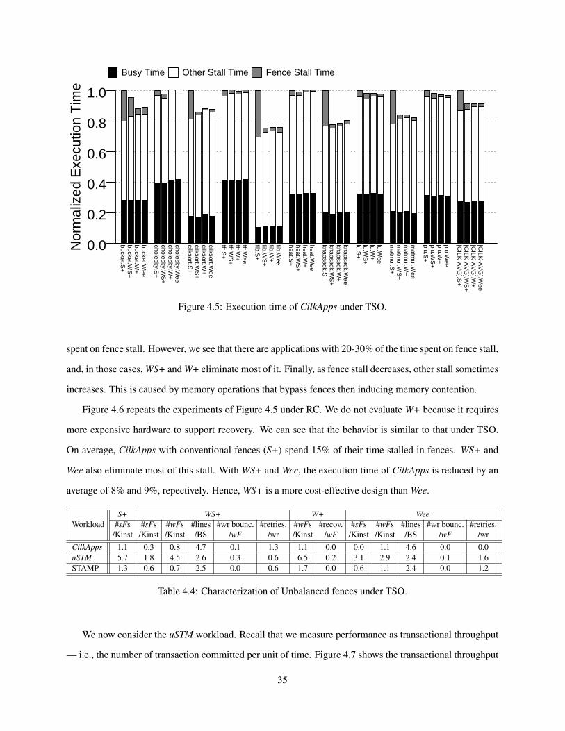
bucket.S+
bucket.WS
+ bucket.W
+ bucket.W
ee
cholesky.S+
cholesky.WS
+ cholesky.W
+ cholesky.W
ee
cilksort.S+
cilksort.WS
+ cilksort.W
+ cilksort.W
ee
fft.S+
fft.WS
+ fft.W
+ fft.W
ee
fib.S+
fib.WS
+ fib.W
+ fib.W
ee
heat.S+
heat.WS
+ heat.W
+ heat.W
ee
knapsack.S+
knapsack.WS
+ knapsack.W
+ knapsack.W
ee
lu.S+
lu.WS
+ lu.W
+ lu.W
ee
matm
ul.S+
matm
ul.WS
+ m
atmul.W
+ m
atmul.W
ee
plu.S+
plu.WS
+ plu.W
+ plu.W
ee
[CILK
-AV
G].S
+ [C
ILK-A
VG
].WS
+ [C
ILK-A
VG
].W+
[CILK
-AV
G].W
ee
0.0
0.2
0.4
0.6
0.8
1.0N
orm
aliz
ed E
xecu
tion
Tim
eBusy Time Other Stall Time Fence Stall Time
Figure 4.5: Execution time of CilkApps under TSO.
spent on fence stall. However, we see that there are applications with 20-30% of the time spent on fence stall,
and, in those cases, WS+ and W+ eliminate most of it. Finally, as fence stall decreases, other stall sometimes
increases. This is caused by memory operations that bypass fences then inducing memory contention.
Figure 4.6 repeats the experiments of Figure 4.5 under RC. We do not evaluate W+ because it requires
more expensive hardware to support recovery. We can see that the behavior is similar to that under TSO.
On average, CilkApps with conventional fences (S+) spend 15% of their time stalled in fences. WS+ and
Wee also eliminate most of this stall. With WS+ and Wee, the execution time of CilkApps is reduced by an
average of 8% and 9%, repectively. Hence, WS+ is a more cost-effective design than Wee.
S+ WS+ W+ WeeWorkload #sFs #sFs #wFs #lines #wr bounc. #retries. #wFs #recov. #sFs #wFs #lines #wr bounc. #retries.
/Kinst /Kinst /Kinst /BS /wF /wr /Kinst /wF /Kinst /Kinst /BS /wF /wr
CilkApps 1.1 0.3 0.8 4.7 0.1 1.3 1.1 0.0 0.0 1.1 4.6 0.0 0.0uSTM 5.7 1.8 4.5 2.6 0.3 0.6 6.5 0.2 3.1 2.9 2.4 0.1 1.6STAMP 1.3 0.6 0.7 2.5 0.0 0.6 1.7 0.0 0.6 1.1 2.4 0.0 1.2
Table 4.4: Characterization of Unbalanced fences under TSO.
We now consider the uSTM workload. Recall that we measure performance as transactional throughput
— i.e., the number of transaction committed per unit of time. Figure 4.7 shows the transactional throughput
35

bucket.S+
bucket.WS
+ bucket.W
ee
cholesky.S+
cholesky.WS
+ cholesky.W
ee
cilksort.S+
cilksort.WS
+ cilksort.W
ee
fft.S+
fft.WS
+ fft.W
ee
fib.S+
fib.WS
+ fib.W
ee
heat.S+
heat.WS
+ heat.W
ee
knapsack.S+
knapsack.WS
+ knapsack.W
ee
lu.S+
lu.WS
+ lu.W
ee
matm
ul.S+
matm
ul.WS
+ m
atmul.W
ee
plu.S+
plu.WS
+ plu.W
ee
[CILK
-AV
G].S
+ [C
ILK-A
VG
].WS
+ [C
ILK-A
VG
].Wee
0.0
0.2
0.4
0.6
0.8
1.0N
orm
aliz
ed E
xecu
tion
Tim
eBusy Time Other Stall Time Fence Stall Time
Figure 4.6: Execution time of CilkApps under RC.
of uSTM for the different Unbalanced fences under TSO. For each microbenchmark, we show bars for S+,
WS+, W+ and Wee fences, all normalized to S+. The rightmost set of bars show the average.
As shown in the figure, WS+, W+ and Wee all outperform S+. This is because, by reducing the fence
stall time, these designs are able to speed-up the execution. On average, WS+, W+ and Wee increase the
transactional throughput by 46%, 58% and 27%, respectively, over S+. We see that W+ and WS+ are much
more cost-effective than Wee.
To understand these results better, Figure 4.7 shows the per-transaction breakdown of processor cycles.
This figure breaks down the bars into the usual categories. Compared to CilkApps in Figure 4.5, these
microkernels spend a much higher fraction of their time in fence stall. On average, with conventional fences
(S+), uSTM spend 54% of their time stalled in fences.
The figure shows that the optimized schemes are very effective. WS+, W+ and Wee eliminate between
half and two thirds of the fence stall time. As a result, the average transaction takes 29%, 35%, and 20%
fewer cycles in WS+, W+ and Wee, respectively, than in S+. W+ is a bit better than WS+, as it reduces
more stall time. However, in part because of its deadlock recoveries, it has a higher busy time than WS+.
36

Counter.S
+ C
ounter.WS
+ C
ounter.W+
Counter.W
ee
DList.S
+ D
List.WS
+ D
List.W+
DList.W
ee
Forest.S
+ F
orest.WS
+ F
orest.W+
Forest.W
ee
Hash.S
+ H
ash.WS
+ H
ash.W+
Hash.W
ee
List.S+
List.WS
+ List.W
+ List.W
ee
MC
AS
.S+
MC
AS
.WS
+ M
CA
S.W
+ M
CA
S.W
ee
ReadN
Write1.S
+ R
eadNW
rite1.WS
+ R
eadNW
rite1.W+
ReadN
Write1.W
ee
ReadW
riteN.S
+ R
eadWriteN
.WS
+ R
eadWriteN
.W+
ReadW
riteN.W
ee
Tree.S
+ T
ree.WS
+ T
ree.W+
Tree.W
ee
TreeO
verwrite.S
+ T
reeOverw
rite.WS
+ T
reeOverw
rite.W+
TreeO
verwrite.W
ee
[uST
M-A
VG
].S+
[uST
M-A
VG
].WS
+ [uS
TM
-AV
G].W
+ [uS
TM
-AV
G].W
ee
0.0
0.5
1.0
1.5
2.0
2.5N
orm
aliz
ed #
Txn
per
sec
Figure 4.7: Transactional throughput of uSTM under TSO.
Interestingly, Wee is not able to reduce the fence stall time as much as WS+ or W+. The reason is that, when
it cannot confine its PS and BS to a single directory module, it turns the fence to sF.
Finally, Figure 4.9 compares the execution time of STAMP applications for different Unbalanced fences
under TSO. The bars are broken down as usual. In the figure, we see a lot of variation. This is because each
application’s potential depends on the amount and type of transactional work that it does.
For example, intruder includes many write operations and, hence, W+ and Wee decrease the fence stall
time more than WS+. Its changes in fence stall also affect the other stall time. labyrinth has very few
transactions in the first place, and hence cannot get noticeable improvements. kmeans and genome see
moderate improvements because most of their stall time is due to reasons other than fences. On average,
with conventional fences, these applications spend 14% of their time stalled in fences. WS+, W+ and Wee
reduce the average execution time by 4%, 11%, and 8%, respectively.
Based on the many applications analyzed, we conclude that W+ is the best scheme under TSO, while
WS+ is the best one under RC. Both are much more cost-effective than Wee. Across all workload sets, WS+
and W+ reduce the execution time over S+ by an average of 14% and 18%, respectively, under TSO.
37

Counter.S
+ C
ounter.WS
+ C
ounter.W+
Counter.W
ee
DList.S
+ D
List.WS
+ D
List.W+
DList.W
ee
Forest.S
+ F
orest.WS
+ F
orest.W+
Forest.W
ee
Hash.S
+ H
ash.WS
+ H
ash.W+
Hash.W
ee
List.S+
List.WS
+ List.W
+ List.W
ee
MC
AS
.S+
MC
AS
.WS
+ M
CA
S.W
+ M
CA
S.W
ee
ReadN
Write1.S
+ R
eadNW
rite1.WS
+ R
eadNW
rite1.W+
ReadN
Write1.W
ee
ReadW
riteN.S
+ R
eadWriteN
.WS
+ R
eadWriteN
.W+
ReadW
riteN.W
ee
Tree.S
+ T
ree.WS
+ T
ree.W+
Tree.W
ee
TreeO
verwrite.S
+ T
reeOverw
rite.WS
+ T
reeOverw
rite.W+
TreeO
verwrite.W
ee
[uST
M-A
VG
].S+
[uST
M-A
VG
].WS
+ [uS
TM
-AV
G].W
+ [uS
TM
-AV
G].W
ee
0.0
0.2
0.4
0.6
0.8
1.0N
orm
aliz
ed E
xecu
tion
Tim
eBusy Time Other Stall Time Fence Stall Time
Figure 4.8: Per-transaction breakdown of processor cycles.
4.5.3 Performance Characterization
Table 4.4 characterizes the S+, WS+, W+ and Wee designs for 8 processors under TSO. Column 2 shows
the average number of sFs per 1,000 dynamic instructions in S+. For CilkApps and STAMP, the number
is around 1, while for uSTM this number is much higher, namely 5.7. Such higher fence frequency is why
WS+, W+, and Wee get better speedups in uSTM.
The next few columns correspond to WS+. Columns 3-4 show the average number of sFs and wFs per
1,000 instructions. The sum of Columns 3 and 4 is equal to Column 2 for CilkApps and STAMP, but not for
uSTM. This is because the uSTM experiments measure throughput and execute slighly different code every
time. For CilkApps and uSTM, wFs are 2-3 times more frequent than sFs. This is why WS+ performs like
W+ in CilkApps and uSTM. However, in STAMP, wFs are as frequent as sFs. Hence, WS+ does not do as
well as W+ in STAMP.
Column 5 shows the average number of line addresses in the BS of a wF. We see that this value is 3-4
for the different workloads. Columns 6-7 consider an average wF and show the average number of writes
that bounce off it and, for each of these writes, the average number of retries until it can commit. In all
cases, the two numbers are low. Hence, the stalls caused by bouncing are largely hidden by the write buffer
38

genome.S
+ genom
e.WS
+ genom
e.W+
genome.W
ee
intruder.S+
intruder.WS
+ intruder.W
+ intruder.W
ee
kmeans.S
+ km
eans.WS
+ km
eans.W+
kmeans.W
ee
labyrinth.S+
labyrinth.WS
+ labyrinth.W
+ labyrinth.W
ee
[ST
AM
P-A
VG
].S+
[ST
AM
P-A
VG
].WS
+ [S
TA
MP
-AV
G].W
+ [S
TA
MP
-AV
G].W
ee
0.0
0.2
0.4
0.6
0.8
1.0
Nor
mal
ized
Exe
cutio
n T
ime
Busy Time Other Stall Time Fence Stall Time
Figure 4.9: Execution time of STAMP under TSO.
and do not cause pipeline stall.
The next two columns correspond to W+. Column 8 shows the average number of wFs per 1,000
instructions. Recall that W+ does not have any sFs. The value is identical to Column 2 for CilkApps, but
larger for uSTM and STAMP because they execute slightly different code. Column 9 shows the average
number of recoveries observed per wF. The value is almost zero for CilkApps and STAMP. However, it is a
significant 0.2 for uSTM. These recoveries are the reason why, in Figure 4.8, the contribution of busy time
and other stall is higher in W+.
Finally, we show data for Wee. Columns 10-11 show the average number of sFs and wFs per 1,000
instructions. Recall Wee only has the equivalent of wFs. However, when a fence’s PS and BS cannot be
confined to a sigle directory module, the fence becomes a sF. We see that, for CilkApps, fences remain wF.
However, for uSTM, about half of the fences turn sF. For STAMP, about one third do. This effect explains
why Wee has a higher fence stall than WS+ and W+ in Figures 4.8 and 4.9. Columns 12-14 show the
number of line addresses in the BS, the number of writes that get bounced per wF, and number of retries
until a bouncing write can commit. These values are similar to those for WS+ (Columns 5-7).
39

4.5.4 Scalability Analysis
Finally, we assess the scalability of Unbalanced fences’ effectiveness to reduce fence stall time. For a given
design (say, WS+), we compare its fence stall time to that of S+. This ratio is shown in Figure 4.10 for
different numbers of processors. The figure organizes the data per workload and fence design. For each
case, it shows bars corresponding to 4, 8, and 16-processor runs. The memory model it TSO.
CilkA
pps-WS
+.P
4 C
ilkApps-W
S+
.P8
CilkA
pps-WS
+.P
16
CilkA
pps-W+
.P4
CilkA
pps-W+
.P8
CilkA
pps-W+
.P16
CilkA
pps-Wee.P
4 C
ilkApps-W
ee.P8
CilkA
pps-Wee.P
16
uST
M-W
S+
.P4
uST
M-W
S+
.P8
uST
M-W
S+
.P16
uST
M-W
+.P
4 uS
TM
-W+
.P8
uST
M-W
+.P
16
uST
M-W
ee.P4
uST
M-W
ee.P8
uST
M-W
ee.P16
ST
AM
P-W
S+
.P4
ST
AM
P-W
S+
.P8
ST
AM
P-W
S+
.P16
ST
AM
P-W
+.P
4 S
TA
MP
-W+
.P8
ST
AM
P-W
+.P
16
ST
AM
P-W
ee.P4
ST
AM
P-W
ee.P8
ST
AM
P-W
ee.P16
01020304050607080
Nor
mal
ized
Fen
ce S
tall
Tim
e (%
)
Figure 4.10: Scalability of the reduction in fence stall time by WS+, W+, and Wee under TSO.
We observe that, for a given workload and fence design, the bars remain fairly flat as we go from 4 to 16
processors. For example, for CilkApps with WS+, the bars remain at 28%. While the total fence stall time
for CilkApps with S+ may change with the processor count, WS+ manages to reduce it always to about 28%
of it. This means that WS+ is scalable. Its effectiveness is not reduced with higher processor counts.
Overall, while the various designs have a different impact on different loads, they all keep their effec-
tiveness across the processor count. Hence, Unbalanced fences are scalable.
40

Chapter 5
Continuous and Precise Recording ofSequential Consistency Violations
5.1 Introduction
An SCV occurs when multiple threads participate in a cycle created by data dependences and program
orders, typically because fences are not inserted sufficiently. SCVs cause a program to execute in totally
counter-intuitive manners, while there are no software techniques for SCV detection and recording.
Data race tools are not precise enough for SCV detection purpose. A data race is only a necessary
condition for an SCV; an SCV requires two or more overlapping data races in a cycle. The very large
majority of data races are not associated with an SCV [32]. Hence, using race-detection hardware would
induce many false positives.
Only enforcing SC rather than also recording SCVs is not enough. The developer needs to know about
SCVs that were avoided, and debug them later, for two reasons. First, a latent SCV may be sign of a deep
bug. Second, we would like the program to also run on off-the-shelf machines correctly.
However, the current hardware schemes that try to detect SCVs [32, 33] reply on expensive hardware
that passes time-stamps of dynamic access through augmented coherence transactions. Also, they have to
terminate the execution after they find the first SCV as the state is already non-SC.
In this section, we will describe SCtame the first hardware architecture for relaxed-consistency ma-
chines that detects and logs SCVs in a continuous manner. With SCtame, as a program executes at production-
run speeds, the hardware records any SCV that occurs (for later debugging) while ensuring that the execution
is always SC. In addition, SCtame is precise (i.e., has no false alarms due to false sharing) and has modest
hardware cost.
41

5.2 SCtame Design
5.2.1 Continuous & Precise SCV Detection
A processor’s SCtame hardware dynamically keeps track of all the out-of-order accesses that are not M-
speculative relative to the consistency model of the machine. Then, it stalls any incoming coherence trans-
action directed to any of these out-of-order accesses. In case of an SCV, these stalls cause a deadlock. Then,
SCtame’s hardware automatically detects the deadlock and logs the SCV — i.e., the deadlocked instruc-
tions’ program counters and addresses accessed.
SCtame then forces at least one of the threads involved in the deadlock to rollback the out-of-order
accesses and re-execute them. During this process, SC is retained. As execution proceeds at production-run
speed, the machine is able to detect and record any future SCVs that occur. These will be true SCVs, not
“artificial” ones that could be induced if SC had not been enforced during the whole process.
As we will see, the SCtame hardware is relatively simple: it is mostly local to each processor, and uses
known mechanisms for state recovery. Moreover, it is scalable.
5.2.2 Reordered Accesses and SCVs
To understand SCtame, we first define the concept of Reordered accesses. Intuitively, these are performed
accesses that are younger than other, incomplete accesses from the same processor, but are allowed by the
memory consistency model to be visible to other processors. Other processors can read and/or invalidate
the data accessed by the Reordered accesses without squashing the Reordered access instructions.
Formally, a Reordered access in a thread is a load or a store instruction for which all of the following is
true:
• Has performed — i.e., for a load, it has deposited the data read into its register and, for a store, the
coherence transaction that it triggered has finished.
• It is preceded in program order by an incomplete memory instruction in the same thread: an earlier
load has not yet performed and retired, or an earlier store has not yet retired and performed.
• It is not M-speculative relative to the memory consistency model supported by the machine. This
means that, if the processor receives an external coherence transaction on the corresponding data, the
42

instruction is not squashed.
Different memory consistency models allow different types of Reordered accesses. In TSO, given an
incomplete store, all the loads that follow in program order, up to (but not including) the oldest unperformed
load are Reordered. In TSO, an incomplete load does not have any Reordered accesses.
In RC, given an incomplete store, all the performed loads and performed stores that follow in program
order are Reordered. Given an unperformed load, all the performed loads that follow are Reordered. (There
cannot be any performed store that follows an unperformed load).
An SCV occurs when two or more processors participate in a dependence cycle. A necessary condition
for a cycle is that a processor (P1) has a Reordered Access (A1) that is seen by another processor (P2).
Hence P2 orders its access (A2) after A1 and does not squash A1. An example is shown in Figure 5.1 for
TSO, where A1 is rd y and A2 is wr y.
A3: rd x
P P1 2
A4: wr x A2: wr y
A1: rd y
Figure 5.1: Example of a pattern that can create an SCV.
This is a necessary but not sufficient condition for SCV. An SCV (for two processors) additionally needs
that P2 issues a subsequent access (A3) that conflicts with an earlier access from P1 (A4) and is ordered
before A4. An example of this pattern is shown in Figure 5.1, where A3 is rd x and A4 is wr x.
5.2.3 Basic SCtame Operation
From the previous discussion, we can deduce the low-cost approach that SCtame uses to detect SCVs:
SCtame stalls accesses that would otherwise observe a reordered access in another processor. In most cases,
the stall will naturally go away as accesses complete. However, if an SCV occurs, the stall will necessarily
cause a deadlock. At that point, SCtame records the SCV, breaks the deadlock, recovers the SC state, and
resumes execution transparently to the program running. We now consider each step, starting with the stall.
To stall accesses, SCtame proceeds as follows:
43

• When an access (A1) in a processor (P1) becomes Reordered, SCtame’s hardware places the address
accessed by A1 and its program counter in a structure in P1’s cache controller called Reordered Set
(RS).
• Coherence transactions received by P1’s cache are checked against its RS for an address match (at
the cache line granularity for realistic hardware). Specifically, incoming reads are checked against the
writes in the RS, while incoming writes are checked against both reads and writes in the RS. If there
is a match, the transaction is refused (i.e., answered with a Nack), which will cause the requester to
retry.
• When A1 ceases to be Reordered, SCtame’s hardware removes it from the RS; it cannot trigger SCVs
anymore.
If a processor runs out of RS entries, it stalls. Also, note that, while an address is in a processor’s RS,
the local cache has to observe all the external coherence transactions directed to the corresponding line.
Hence, we need to consider the evictions of lines with RS entries from the cache. If the line is clean, it can
be evicted silently, since future coherence transactions will still be observed locally (in directory protocols,
because the directory has not been notified; in snoopy protocols, because invalidations are broadcasted).
If, however, the evicted line is dirty and the machine uses directory-based coherence, special care is
needed, since the visibility of future coherence transactions is in jeopardy. Hence, in this case, SCtame rolls-
back to the state before the instruction that created the RS entry. In practice, cache replacement algorithms
that follow LRU-like policies rarely choose to evict a line with a recently-inserted RS entry.
Consider Figure 5.1. Assume load A1 performs before store A4 completes and address y is placed in
P1’s RS. Later, store A2 executes, initiating a coherence transaction that reaches P1’s cache and hits in the
RS. The transaction bounces, preventing P2 from executing A2. When store A4 drains from the write buffer,
address y is removed from P1’s RS. A retry of store A2 by P2 now succeeds. However, if the timing is such
that A2 waits on A1, and A4 waits on A3, we have stumbled on an SCV, and the system deadlocks; SCVs
always cause deadlocks.
Section 5.3.1 describes the RS operation in detail.
44

5.2.4 Types of Stalls
SCtame’s stalls can be classified based on whether or not they cause deadlocks (Table 5.1). In most cases, a
stall is temporary, and, therefore, does not cause deadlock. The stall goes away after an access completes and
what used to be its Reordered accesses are removed from the RS. These stalls do not flag SCVs (Table 5.1).
No Deadlock DeadlockTrue Dependences False Sharing
SCV? No Yes No
Table 5.1: Relationship between deadlocks and SCVs in SCtame.
When stalls cause a deadlock, it is possible that there is an SCV. In an SCV involving N processors,
we have N processors stalling one another in a cycle — each processor waiting on another processor’s RS,
and hence deadlocked. Examples of two- and three-processor cycles under RC are shown in Figures 5.2(a)
and (b), respectively. In the figures, the addresses in the RS are shown in a box, and a bouncing access is
represented by an arrow that curves back to its source.
P P1 2
A4: wr x
xyRS RS
A3: rd xA1: wr y
A2: rd y
(b)
(a)
PP
x RSRS
P1
yRS
A1: rd y
2 3
A6: wr x A2: wr y
A3: rd z
z
A4: wr z
A5: wr x
Figure 5.2: Examples of deadlocks caused by SCVs.
False sharing at the cache line level can also cause a deadlock (Table 5.1). Since processors initiate co-
herence transactions at cache-line granularity, requests are bounced even though the accesses are to different
words of the same line. For example, this is shown in Figure 5.3(a), where words a and b share a line. As
we will see, SCtame detects this case, breaks the deadlock, restores SC, and continues without recording
45

any SCV.
(b)
P1
RS
P2
wr x
rd a
a
wr b
rd x
x RS
x RS
P1
yRS
P2
P3
wr x
rd y
wr y
rd x
wr x
(a)
Figure 5.3: Other cases of deadlocks.
Note that when there is a deadlock (due to true dependences or false sharing), it is possible that a
processor that does not participate in the cycle also gets embroiled in the deadlock. This occurs when the
processor accesses an address that is already part of a cycle in other processors. An example is processor P3
in Figure 5.3(b). In this case, when SCtame breaks the deadlock (Section 5.2.7), the processor gets released.
Overall, SCtame is precise because of two reasons. First, SCtame records all the SCVs that occur (for
a given dynamic execution of the program). This is because all SCVs cause deadlocks. Second, SCtame
only records true SCVs. The reason, as we will see, is that SCtame identifies the deadlocks caused by false
sharing, and silently recovers from them.
5.2.5 Detecting a Deadlock
A sign that a processor Pi may be participating in a deadlock is that its RS bounces an external request, and
one of its own requests is being bounced by another processor. However, SCtame initiates the Deadlock
Detection and Analysis (DDA) algorithm in Pi only if and when it is Pi’s oldest incompleted access (Aold i)
the one bounced by another processor. In TSO, Aold i is the write at the head of the write buffer; in RC,
Aold i is such a write or, if the write buffer is empty, the read at the head of the ROB. Attempting the
detection any earlier is unproductive since, in reality, we may not be in a deadlock.
46

At a high level, when Pi bounces an external request and its Aold i access is being bounced, SCtame
embeds some information in Pi’s future Aold i retry messages. Such information will propagate to all the
processors involved in the potential cycle. If the information ever reaches back to Pi, it means that there is
a cycle. Then, Pi records the local SCV state and adds further information to its retry messages. When this
additional information reaches back to Pi, it means that all the processors in the cycle have recorded the
SCV. Then, Pi initiates recovery.
The information included in a retry message is: (1) two bitmaps (Round0 and Round1) with as many bits
as processors in the machine, which will record the processors participating in the cycle; (2) the fine-grain
address (Addr) of the byte or word accessed by Aold; and (3) a bit (FS) that records whether the cycle is due
to false sharing. All request messages contain these fields, but they are ordinarily unused.
DDA starts when Pi was bouncing an external request and its Aold i access is bounced. At this point,
SCtame includes in Pi’s future Aold i retry messages: (1) Round0 with bit i set, (2) an empty Round1 bitmap,
(3) Addri set to the word (or byte) address accessed by Aold i, and (4) FS set to zero.
The processor at the receiving end (Pj) simply ignores this information if its own Aold j is not being
bounced. However, if it is, SCtame performs two actions. First, it checks if the Addri in the message
matches an address in Pj’s RS exactly or only because of false sharing in the same cache line. If the latter
is true, Pj sets a local FS bit. Second, Pj includes in its own Aold j retry message: (1) Round0 coming from
Pi augmented by also setting the j bit, (2) Round1 coming from Pi; (3) the fine-grain address that Aold j
accesses (Addrj), and (3) the FS bit coming from Pi OR-ed with the locally-generated FS bit.
Successive processors in the cycle perform the same two actions. Note that it is possible that multiple
processors in a given cycle start the DDA algorithm at the same time; the algorithm works equally well.
If there is a cycle, Pi eventually finds that it is bouncing an incoming request with its own ID bit already
set in Round0. Hence, we have a deadlock. Pi also computes its local FS bit. If the incoming message’s
FS bit or the local FS bit is set, the cycle is due to false sharing. In this case Pi simply initiates recovery
(Section 5.2.7).
Otherwise, the cycle is due to true dependences. Then, Pi records the local SCV state (Section 5.2.6).
In addition, in future retries of Aold i, in addition to including the usual information, Pi sets the i bit in
Round1. The same operation is performed by all the other processors in the cycle. Therefore, a second
wave of information traverses the cycle. Finally, when Pi finds that it is bouncing an incoming request with
47

its own ID bit already set in both Round0 and Round1, it knows that all the processors in the cycle have
recorded their local SCV state. At this point, Pi initiates the recovery.
For a given cycle, it is possible that more than one processor initiate DDA. In this case, more than one
processor can initiate the recovery. However, each processor in the cycle logs the local SCV state only once.
Section 5.3.2 describes the DDA algorithm in detail.
Figure 5.4 shows an example of DDA for four deadlocked processors due to true dependences. In the
figure, only P0 initiates DDA. For each message, the lighter bitmap is Round0, while the darker one is
Round1. The numbers in parenthesis show the temporal sequence of events. While each processor continu-
ously issues retry messages, each chart only shows one retry per processor. In Chart (a), as information is
propagated from P0 to back to P0, each processor populates Round0. In Chart (b), each processor finds its
bit set in Round0, logs the SCV state, and populates Round1. Finally, Chart (c) shows what happens after
P0 has received message (8), as will be explained in Section 5.2.7. In this case, P0 initiates recovery (9)
and, as a result, the next retry from P3 succeeds (10).
P0
P1
P3(c)
(9)
(10)
0 0 0 10 0 0 0 0 0 0 0
0 0 1 1
0 0 0 00 1 1 1
0 0 0 0 1 1 1 1
1 1 1 10 0 0 1
1 1 1 10 0 1 1
1 1 1 10 1 1 1
1 1 1 11 1 1 1
P2
P1
P3(b)
P0
log P2log
(5)(6)
(7)(8)
Success
P0
P1
P2
P3(a)
(1) (2)
(3)(4)
log
log
Recovery
Figure 5.4: Example of deadlock detection and analysis.
5.2.6 Recording the SCV
As indicated above, when a processor Pi bounces for the first time an incoming access that contains Round0
with bit i set and Round1 with bit i clear, and there is no false sharing, SCtame records the local SCV
state. Specifically, SCtame dumps four pieces of information into a memory in the cache controller: the
program counter (PC) and the address accessed by the two local instructions involved in the SCV. One
of the instructions is Aold i (the access being bounced, such as A4 in Figure 5.2(a)). Its PC and address
are readily available. The other instruction is the one that created the RS entry that bounces the incoming
coherence request (such as A1 in Figure 5.2(a)). We identify the RS entry as the one that exactly matches
48

the address in the incoming bounced request. RS entries contain both the address and the PC.
A processor’s recording operation is unlikely to take more than several tens of cycles and, therefore,
induces a negligible performance impact.
5.2.7 Recovery from SCVs while Retaining SC
As discussed before, when a processor Pi bounces an incoming request where bit i is set in both Round0
and Round1, Pi initiates recovery. The goal is to return the deadlocked processors to production execution
transparently right away. The recorded SCV information can be analyzed off-line later.
To understand the recovery, note that the state of the global memory system at this point is the one before
Aold k for all the k processors participating in the deadlock. However, the pipeline state of each processor
k is beyond this point. Hence, to recover from the deadlock while retaining SC, we need for at least one
of the k processors (e.g., Pi) to roll back its pipeline state to when the bounced request (Aold i) was at the
head of its ROB. This will roll back its Reordered accesses and clear its RS, allowing the other deadlocked
processors to make progress. At the same time, Pi can re-execute Aold i and subsequent instructions. This
approach is attractive because it only requires logic that is local to the processor, and is compatible with
common pipeline-recovery mechanisms.
Specifically, recovery in a processor involves rolling back all the instructions that have been retired from
the ROB since the still-incompleted Aold access. These instructions can be of all types, and may include
stores. To roll back, SCtame uses a History Buffer (HB) circular queue [42], which has already been used
for recovery in previous proposals (e.g., [19, 35]) with different designs. SCtame uses an HB design that
can have multiple retired writes. Recall that the HB temporarily stores the processor state that each of the
retired instructions over-writes. As an instruction retires from the ROB, if there is an incompleted older
access, the hardware fills an entry at the tail of the HB. Each entry contains the old value and the mapping
of the register that the instruction writes. It also includes the instruction’s PC.
For simplicity, SCtame does not store speculatively-generated state in the caches. A reordered store
keeps its state in the write buffer, and triggers an exclusive prefetch to the cache, to bring the corresponding
line in Exclusive mode into the cache. When the prefetch completes, the store is considered performed, and
is entered in the RS. In this way, when stores are eventually merged in order with the memory system, they
can do so very quickly, while their rollback before that point is simple. The actual recovery process under
49

TSO or RC is described in Section 5.3.3.
Livelock Considerations.
In the example of Figure 5.4, P0 rolls back in step (9). This operation clears its RS, which enables the access
from P3 to succeed (step (10)). As P3 makes progress, P1 and P2 will also likely make progress without
suffering a rollback.
Depending on the timing, it is possible that multiple processors in a cycle (or all of them) perform
rollbacks concurrently — either because they initiated DDA at the same time or due to other timing reasons.
The algorithm works correctly in all cases. As multiple processors re-execute their Aold accesses again,
they are very unlikely to get into the same deadlock. However, if that happens, SCtame recovers again. To
absolutely guarantee forward progress, we could use a simple technique: after deadlock recovery, we could
force the processors to execute the Aold access without allowing any reordering. In this way, processors
would make guaranteed progress. In our current SCtame design, we do not use this technique and always
observe forward progress.
5.3 Hardware Implementation
In this section, we describe the operation of three components of SCtame: Reordered Set (RS), DDA, and
History Buffer (HB). Then, we examine SCtame’s hardware complexity.
5.3.1 RS Implementation and Operation
The RS is a hardware structure in the cache controller that stores the addresses accessed by the current
Reordered accesses in the processor. Each entry contains the address, the PC of its instruction, and some
additional state. New entries are dynamically added and removed. The RS is organized as a circular FIFO
queue, ordered in program order of the Reordered accesses. In this section, we describe its operation under
TSO and under RC.
Operation under TSO Hardware.
Given an incomplete store, its Reordered accesses are all the loads that follow it in program order, up to (but
not including) the oldest unperformed load. An incomplete load has no Reordered accesses.
50

From this discussion, the RS can only contain loaded addresses. Moreover, when a store completes,
we need to remove from the RS the addresses for all the subsequent loads until the next incomplete store.
Hence, to speed-up RS operation, we design SCtame as follows. Each instruction in the ROB has a Write
Tag (WT). When a store is inserted in the ROB, its WT is set to the value of the previous instruction’s WT
plus one. For non-store instructions, the WT is that of the previous instruction. Hence, all the instructions
following a store have the same WT, which is different from those following the next store, and so on. The
WT is also stored in each RS entry.
The algorithm to insert entries in the RS tail and remove them from the RS head is as follows. When a
load (l1) performs and (i) there is a store older than l1 that is incomplete (it can be still in the ROB or already
retired in the write buffer) and (ii) there is no unperformed load older than l1 in the ROB, then:
• The address loaded by l1 is inserted in the RS.
• The addresses loaded by all the loads ln that follow l1 in program order up to (but not including) the
oldest unperformed load are also inserted in the RS in program order.
Entries are removed when a store completes. In this case, all the loads in the RS with the same WT as
the write are removed. We stop when the RS is empty or we find a load with a different WT (which follows
the next incomplete store).
Operation under RC Hardware.
Given an incomplete store, its Reordered accesses are all the performed loads and all the performed stores
(i.e., those that have completed the Exclusive prefetch) that follow it in program order. Moreover, given an
unperformed load, its Reordered accesses are all the performed loads that follow it in program order.
Hence, both loads and stores can be in the RS. Moreover, any performed accesses that are preceded by
unperformed ones need an RS entry. These facts make the hardware costlier, but the insertion and removal
algorithms simpler. Indeed, as a load or a store is entered in the ROB, SCtame reserves an (empty) entry for
it at the tail of the RS. Then, actual insertions or removals of addresses to/from the RS can only occur at a
single point: when an access a1 (load or store) performs.
Specifically, when a1 performs, if there is at least one non-performed access older than a1, then the
address accessed by a1 is inserted in its reserved entry in the RS. Otherwise, a1 was the oldest non-performed
51

access and was at the RS head. In this case, no entry is allocated and, starting at the RS head and moving
backwards, all the entries in the RS are removed in order until the first entry that is still empty (which
corresponds to an unperformed access).
5.3.2 The DDA Algorithm
When the Aold i access of a processor Pi is being bounced, and Pi receives an incoming request that bounces
in its RS, its SCtame hardware runs the DDA algorithm of Figure 5.5. If the incoming request does not
contain deadlock information (Line 1), then Pi starts deadlock detection by including, in its Aold i retries,
the data structures shown in Figure 5.5. As shown in Line 2, the values included are: bit i set of Round0, a
null Round1, the fine-grain address of Aold i, and a clear FS bit.
Round0 Round1 Addr FS
3 else { /* this proc does not start DDA */4 if (hit due to false sharing)5 local_FS =1
9 }
11 if (FS | local_FS == 0) { /* cycle with only true dependences */
13 Record SCV /* record the local SCV state */
15 }
17 Recover (P_i) /* start recovery for proc P_i, which breaks the cycle */18 }19 }20 else { /* false sharing cycle; first detection */
22 }23 }24 }
16 else { /* 2nd round completed now */
1 if (incoming request has no info) { /* this proc starts DDA */2 Include in A_old_i msg (i, null, Addr_i, 0)
8 Include in A_old_i msg (Round0 |= i, null, Addr_i, FS |= local_FS)
6 if (i bit is not set in incoming Round0){ 7 /* this proc hasn’t informed all the other procs in the cycle about its participation */
10 else { /* information has propagated around the cycle */
14 Include in A_old_i msg (Round0, Round1 |= i, Addr_i, 0) /*start 2nd round*/
12 if (i bit is not set in incoming Round1) { /* only 1st round completed */
21 Recover (P_i) /* breaks the cycle; no recording of SCV */
Figure 5.5: The DDA algorithm, as executed by Pi.
Otherwise, deadlock detection is already in progress (Line 3). In this case, Pi first checks if it is bouncing
an access due to false sharing (Line 4) and, if so, sets the local FS bit (Line 5). Moreover, if bit i is not
yet set in the incoming Round0 (Line 6), it means that Pi has not yet informed all the other processors
52

in the potential cycle about Pi’s participation in the cycle. Therefore, SCtame takes the information in
the incoming bouncing message, augments it, and includes it in future Aold i retries. This augmentation
involves setting bit i in Round0, keeping Round1 null, enclosing the fine-grain Aold i address, and OR-ing
the local FS bit to FS (Line 8).
If bit i is set in the incoming Round0 (Line 10), we have a cycle and the information has propagated
around the cycle. SCtame first checks if any processor (including Pi) detected false sharing (Line 11). If
so (Line 21), Pi recovers. Otherwise, SCtame checks if the information has gone around the cycle once
or twice. If the former, SCtame records the local SCV state (Line 13) and augments the retry messages by
setting bit i in Round1 (Line 14). If the latter, since all processors have recorded the SCV, SCtame initiates
the recovery (Line 17).
5.3.3 HB Operation and Recovery
The recovery is different in a machine supporting TSO or RC.
HB Operation and Recovery under TSO.
The stalled Aold instruction is the oldest retired, incomplete store at the head of the write buffer. When such
store completes, SCtame tries to free HB entries. Starting from the HB head, it walks backward, freeing all
the entries with the same WT as the completed store, stopping at the first entry with a different WT or when
the HB is empty. At this point, if a new store is at the HB head, that store can proceed to update the cache;
hopefully, the exclusive prefetch has already brought the line, and the store can drain immediately. Recall
that, under TSO, the stores have to be merged in program order.
Recovery for a processor starts by first clearing the RS, write buffer, and ROB. Then, starting from the
HB tail and walking toward older instructions, each HB entry is used to undo the state changes performed
by the corresponding instruction. After the whole HB is applied, the processor has the correct state, and the
hardware attempts to perform the Aold access again.
HB Operation and Recovery under RC.
The stalled Aold instruction can be either (i) the oldest retired, incomplete store at the head of the write buffer
or (ii) the oldest unretired load at the head of the ROB. Under RC (and unlike TSO) the stores that retired
53

after an incomplete Aold store at the head of the write buffer could be performed and completed out of order
relative to Aold. However, recall that, since we may have to roll them back in case of a recovery, SCtame
does not perform them. Instead, SCtame follows the same strategy as in TSO: the stores are left in the write
buffer without being merged with memory, while an exclusive prefetch is sent out. With this design, HB
operation is simple: when the oldest store completes, SCtame walks backward in the HB, freeing the entries
of all the completed accesses until either the HB is empty or the next incompleted write is found.
Recovery has only one small difference relative to TSO. Specifically, if Aold is the oldest unretired load
at the head of the ROB, the HB is empty, and there is no HB to apply.
5.3.4 Hardware Complexity
The hardware required by SCtame is of modest complexity, especially when compared to other SCV detec-
tion schemes such as Vulcan [32] and Volition [33]. It has three components: the RS, the DDA mechanism,
and the HB.
The RS is a small circular FIFO queue in the L1 cache controller. Each entry has an address, a PC
and, under TSO, a WT. Entries are allocated when accesses become Reordered, and deallocated when
they cease to be Reordered. Incoming requests are compared to the RS addresses. For efficiency, the RS
is not implemented as a CAM. Instead, we perform sequential comparisons, 4 entries at a time. This is
reasonable because this operation is not time-critical, and because there often are very few RS entries in
use. For instance, the RS evaluated in Section 5.4 has 32 entries, but it on average it uses only 6.3. A further
optimization involves using a Bloom filter.
The DDA mechanism consists of an FSM in the L1 cache controller that examines some incoming
messages and updates some outgoing ones. Specifically, it reads information from incoming messages that
bounce in the RS, and sets bits in outgoing retry messages. All request messages now include two processor
bitmaps, a few bits to identify which word of the line was accessed, and an FS bit. For a 16-processor
machine with 32-byte cache lines, this amounts to 5 bytes. Each FSM operates independently and can
declare a cycle locally.
Request bouncing simply means that a message failed and the FSM at the sender is informed that it
needs to retry. Being a null transaction that had no side-effects, it does not impose any restriction on the
coherence protocol. Beyond the extra bits per request and request bouncing, there is no other change to
54

the coherence protocol: no new messages, new states, or new transactions. There are no changes to the
directory module.
Finally, each processor has an HB circular queue for recovery of retired instructions that follow an
incomplete access. Each HB entry has a register value, a register mapping, and a PC. An HB entry is
filled quickly with minimal computation, although it requires a register read. For simplicity, no speculative
updates go into the L1 caches. Rollback involves undoing one instruction at a time, but it happens rarely.
Overall, the SCtame hardware is mostly local to each processor node and, in part, uses known recovery
techniques.
5.4 Experimental Results
5.4.1 Experiment Setup
We evaluate SCtame’s ability to detect SCVs in multithreaded programs running on RC or TSO hardware.
We also evaluate SCtame’s performance overhead. We perform detailed cycle-level execution-driven sim-
ulations. We model a multicore with 16 processors connected in a mesh network with a directory-based
MESI coherence protocol. Each core has a private L1 cache and a bank of a shared L2 cache. SCtame adds
a History Buffer (HB) to each core and a Reordered Set (RS) to each L1 controller. In addition, it augments
each request message leaving the L1 cache with 5 extra bytes (Section 5.3.4). In this evaluation, the RS
stores word addresses. Table 5.2 shows the architecture parameters. From the table, it can be seen that the
storage needed by the SCtame hardware is modest.
Architecture 16-core multicoreCore Out of order, 3-issue wide, 2.0 GHzROB; write buffer 140-entry; 64-entryL1 cache Private 32KB WB, 4-way, 2-cycle RT, 32B linesL2 cache Shared 2MB WB with 16 128KB banks
Bank: 8-way, 11-cycle RT (local), 32B linesCache coherence MESI, full-mapped directoryOn-chip network 4x4 2D-mesh, 5 cycles/hop, 256bit linksOff-chip memory Connected to one network port, 200-cycle RT
Reordered Set 32 entries/proc: 8B addr + 1B WT + 8B PCHistory Buffer 64 entries/proc: 8B reg + 2B map + 8B PCRetry delay 20 cycles before issuing a retry messageRecording an SCV 5 cycles of overhead
Table 5.2: Architecture modeled. RT stands for round trip.
55

To evaluate SCtame’s ability to detect SCVs, we use a set of 12 programs [7, 8, 15] that implement
concurrency algorithms, such as a lock-free queue and a work-stealing queue. We remove the fences in
these codes and, therefore, their execution may violate SC on plain RC or TSO hardware. Each thread in
each program executes a loop with 200 iterations that accesses shared data structures. We call them kernels
(Table 5.3).
bakery Mutual excl. algorithm for arbitrary # of threadsdekker Mutual excl. algorithm for two threadsharris Non-blocking setlazylist Concurrency list algorithmtakequeue Cilk THE work stealing algorithmaharr Variant of harrismoirbt Non-blocking sync. primitivesmoircas Non-blocking sync. primitivesms2 Two-lock queuesnark Non-blocking double-ended queuemsn Non-blocking queuemst Non-blocking queue
Table 5.3: Kernels that implement concurrency algorithms.
RC TSOCode SCtame IF IF-CoV SCtame IF IF-CoV
#SCV #Stall #Squash #Timeout #Stall #SCV #Stall #Squash #Timeout #Stallbakery 3 4494 5630 254 6647 3 4362 4583 6 6980dekker 14 91412 76471 29 60961 17 83093 85603 21 58183harris 302 23256 25885 2012 32792 191 24010 21723 1679 33210lazylist 162 8845 8840 1039 9105 75 7946 8166 798 9466takequeue 165 6980 6856 993 6731 98 6905 6816 788 6319aharr 100 11525 11593 859 11494 74 10546 11504 803 11602moirbt 218 9373 10381 1293 9459 143 8775 10893 1015 8522moircas 149 5648 7964 843 9667 35 5225 6189 616 10833ms2 193 19039 21907 1509 23244 145 17676 20831 1102 22837snark 10 9431 14636 143 15855 13 9786 13262 180 17495msn 2 8322 7302 35 6715 0 7676 7829 26 6222mst 3 7927 9527 28 10663 0 7765 8230 21 12102
Average 110 17188 17249 753 16944 66 16147 17136 588 16981
Table 5.4: SCV detection for the kernel programs.
SCtame detects and records SCVs precisely during the execution, and recovers from an SCV while
retaining SC. We compare SCtame to an SCV-detection scheme that, when an SCV is found, terminates
execution because SC cannot be maintained. Examples of such a scheme are Vulcan [32] and Volition [33].
We also compare SCtame to two SC-enforcing-only schemes: InvisiFence [5] with and without Commit on
Violation (we call them IF and IF-CoV). Such schemes are conservative in that they squash execution as
56

soon as a certain necessary condition for an SCV occurs. They are not usable to report SCVs because they
would report many false positives (Section 2.4). IF-CoV uses a 4,000-cycle timeout threshold.
To evaluate the performance overhead of SCtame over plain RC or TSO hardware, we also use 16
programs from SPLASH-2 [46] and PARSEC [4]. We call these programs apps. Apps run correctly on RC
or TSO hardware, but SCtame can induce performance overhead as it tries to conservatively enforce SC.
5.4.2 SCV Detection
Number of SCVs Detected.
To assess SCtame’s ability to detect and record SCVs, we run the kernels under RC and TSO. We report the
number of SCVs and the number of accesses stalled. The apps are found to have practically no SCV, and
so they are not shown. For comparison, we also run the kernels with IF and IF-CoV. Since these schemes
cannot observe SCVs, we report the number of squashes (in IF), and stalls and timeouts (in IF-CoV). The
data is shown in Table 5.4, where RC data is on the left and TSO data on the right.
Consider the RC environment. Column 2 shows the number of dynamic SCVs detected by SCtame.
We see that SCtame detects SCVs in all the kernels. On average, it detects 110 SCVs. Column 3 shows
the number of dynamic accesses stalled by SCtame. Such number is more than 100 times higher than the
number of SCVs. Most of these stalls are very short and unrelated to an SCV. This shows that seeing a
single access reorder from another processor (i.e., a data race) is not a good SCV indicator; one needs to see
a dependence cycle.
Column 5 shows the number of squashes in IF. This number is similar to the stalls in SCtame — but not
exactly the same because the memory accesses interleave slightly differently. It is, however, much higher
than the number of SCVs. Finally, Columns 6 and 7 show the number of timeouts and stalls in IF-CoV.
The number of stalls is also similar to SCtame. The number of timeouts is closer to the number of SCVs,
but much higher for two reasons. First, as we will see, most timeouts are caused by false sharing of cache
lines. Second, when a group of processors times out, this counter increases by the number of timed-out
processors. In any case, IFCOV’s timeouts are unable to record information useful to debug SCVs.
The data for the stronger TSO is similar, with a lower number of SCVs. Overall, this section shows
that SCtame successfully finds SCVs, and that conventional SC-enforcement approaches cannot be used for
SCV detection and debugging.
57

Stopping versus Continuing.
Unlike SCtame, other precise SCV detection schemes such as Vulcan [32] and Volition [33] terminate
execution once they find an SCV. They are unable to retain SC execution and, therefore, they could find
additional artificial SCVs caused by the non-SC execution. We call them Stop approaches. Debugging with
them involves multiple iterations of: SCV detection, termination and fixing the SCV by inserting fences,
and then re-execution from the beginning of the application. It usually takes several runs to detect the SCV
bugs that SCtame detects in a single run. Also, these schemes are incompatible with production runs.
We compare SCtame to the operation of SCtame with the Stop approach. In this case, each re-execution
finds one SCV, which is fixed with fences. Table 5.5 compares the number of runs to detect all the SCVs in
the kernels for the two approaches, using RC. This table differs from Table 5.4 in that we perform as many
runs as needed to find all SCVs (Table 5.4 corresponds to only one run). We see that Stop typically requires
several runs to find all the SCVs. SCtame only needs one run or, in three kernels, two.
Code SCtame Stop Code SCtame Stop
bakery 1 1 dekker 1 1harris 1 6 lazylist 1 4takequeue 1 6 aharr 1 7moirbt 1 3 moircas 1 4ms2 1 2 snark 2 14msn 2 9 mst 2 8
Table 5.5: Number of runs to find all SCVs in RC.
Sensitivity Study.
We examine the sensitivity of SCV detection to the size of the RS and the size of the write buffer. As the
size of the RS or write buffer increases, the degree of reordering of memory operations increases, which
leads to more SCVs. The results are shown in Figures 5.6 and 5.7 for both RC and TSO hardware. The
figures show the average number of SCVs observed per kernel for 16-processor runs.
In Figure 5.6, we change the RS size from 2 to our default of 32. In Figure 5.7, we change the write
buffer size from 4 to our default of 64. We can see that, as the hardware becomes more aggressive, SCtame
detects more SCVs. Also, RC systems always detect more SCVs than TSO ones. Overall, we choose our
default sizes based on when the curves saturate.
58

2 4 8 16 320
30
60
90
120A
vera
ge N
umbe
r of
SC
Vs
RCTSO
Figure 5.6: RS size.
4 8 16 32 640
30
60
90
120
Ave
rage
Num
ber
of S
CV
s
RCTSO
Figure 5.7: Write buffer size.
5.4.3 SCtame Execution Time Overhead
Compared to conventional hardware, SCtame incurs two types of execution overhead. The first is access
stall overhead, which is caused by accesses that hit in the RS of other processors and have to retry. The
second overhead is recovery from deadlock. This operation requires restoring the architectural state by
traversing the HB and flushing the pipeline.
Figure 5.8 shows the execution time of SCtame for apps normalized to the execution time on plain
RC hardware. The bars are labeled S. As a reference, we also show bars for the IF-CoV scheme for SC
enforcement. The bars are labeled I. The bars are broken down into categories. SCtame has Recovery
(overhead of accesses that deadlock, including their stall, recovery, and re-execution), Stall (overhead of
stalls that do not deadlock), and Useful (rest of the time). IF-CoV has Timeout (overhead of accesses that
timeout, including their stall, squash, and re-execution), Stall (overhead of stalls that do not timeout), and
Useful. Squash in IF-CoV uses a cache flash clear.
The figure shows that, on average, the stall cycles are only about 2% of the cycles in both schemes. The
stall is small because the latency of access bouncing is partially hidden by the execution of other instructions.
In addition, recovery and timeout cycles are practically zero. This is because there are very few dependence
cycles in these codes. Overall, SCtame induces an average overhead of ≈2% over RC. This is a largely
negliglible overhead, and an acceptable cost to ensure SC. The average overhead of IF-CoV is similar. A
similar result can be shown for TSO. We note that a few codes have a larger stall time. These are codes with
fine-grain sharing, where the dependence cycles are due to false sharing.
We now consider the kernels. Since we removed the fences from these codes, they may run incorrectly
59

80
90
100
110E
xecu
tion
Tim
e B
reak
dow
n (%
)Timeout Recovery Stall Useful
I Sbarnes
I Sfm
mI Socean
I Sradio
I Sraytrace
I Swater-ns
I Swater-sp
I Scholesky
I Sfft
I Sradix
I Sblack
I Scann
I Sdedup
I Sfluid
I Sstream
I Sswap
I Savg
Figure 5.8: Execution time of apps with IF-CoV (I) and SCtame (S) on RC. The bars are normalized toplain hardware.
on plain RC or TSO hardware. Hence, we only compare the execution time of SCtame to IF-CoV. Figure 5.9
shows the execution time of the kernels for IF-CoV (labeled I) and SCtame (labeled S) on RC. The bars are
normalized to IF-CoV and broken down as above.
With plain RC or TSO hardware, access reordering by the hardware would cause SCVs. With SCtame,
it causes stalls and recoveries. The figure shows that, on average, the stall cycles in SCtame are about 5%.
Recovery time is also visible. With IF-CoV, we see stalls and timeouts. On average, SCtame has a very
small execution time advantage over IF-CoV. A similar result can be shown for TSO. Overall, therefore, the
key capability of SCtame, namely continuous and precise detection and recording of SCVs, does not come
at the expense of any slowdown relative to an SC-enforcing-only scheme such as IF-CoV.
5.4.4 SCtame Characterization
Table 5.6 characterizes SCtame for all the programs on RC. We do not show a characterization on TSO due
to lack of space. Columns 2-3 show the average and maximum number of entries used in the RS during
execution. On average, the RS size is only around 6 entries for both kernels and apps. It can be shown that
the corresponding number for TSO is ≈3. Columns 4-5 consider the reads and writes that are bounced due
to a hit in an RS. The columns show, in order, the number of such accesses per 10K accesses, and the average
number of cycles between the first bounce at an RS entry and the deallocation of that RS entry. As we can
see, for the large majority of codes, the rate of bounced accesses is very low. In addition, the duration of the
60

60
70
80
90
100E
xecu
tion
Tim
e B
reak
dow
n (%
)Timeout Recovery Stall Useful
I Sbakery
I Sdekker
I Sharris
I Slazylist
I Stakequeue
I Saharr
I Sm
oirbt
I Sm
oircas
I Sm
s2
I Ssnark
I Sm
sn
I Sm
st
I Savg
Figure 5.9: Execution time of kernels with IF-CoV (I) and SCtame (S) on RC. The bars are normalized toIF-CoV.
stall in an RS entry is only a few tens of cycles. The rate of bounced accesses does not correlate perfectly
with the SCtame stalls in Figures 5.8 and 5.9; other factors like the access rate or clustering have an effect
as well.
Columns 6-7 consider the reads and writes that are involved in a cycle and trigger a recovery. The
columns show the number of such accesses per 10K accesses, and the percentage of such cycles caused by
false sharing. We can see that recoveries are much rarer than bouncing events: on average, 20x rarer in
kernels and 32x in apps. In addition, most of the dependence cycles in the kernels (83% on average) and
practically all of those in the apps are due to false sharing. Hence, supporting a precise scheme like SCtame
is crucial. Finally, it can be shown that the traffic increase due to SCtame is negligible.
5.4.5 SCtame Scalability Analysis
Figure 5.10 shows the execution time overhead of SCtame over plain RC and TSO hardware for 8, 16 and
32 processors for the apps. We only show a sample of the apps and the average of all apps. We see that,
with increased numbers of processors, the overhead of SCtame does not change much and stays, on average,
around 2% for both RC and TSO. This shows that SCtame is scalable.
61

Reordered Bounced Reads Recovery ReadsCode Set Size & Writes & Writes
Avg Max #/10K Cyc. #/10K FS(%)
bakery 3.0 32 489.8 45.0 32.5 87.3dekker 11.0 32 270.3 42.2 11.1 92.2harris 6.7 19 30.3 69.7 2.0 79.5lazylist 2.7 16 33.8 20.0 2.0 81.4takequeue 5.0 32 156.0 33.1 5.4 68.0aharr 2.0 15 30.8 35.6 0.4 77.4moirbt 8.5 32 138.2 54.7 6.6 91.2moircas 7.2 32 124.8 34.5 3.8 93.9ms2 3.2 27 297.9 34.4 16.2 73.8snark 5.5 12 0.3 26.6 0.0 89.4msn 12.0 30 7.2 39.2 0.0 94.5mst 8.2 19 13.2 17.2 0.0 69.6
Average 6.2 24.8 132.7 37.6 6.6 83.2
barnes 10.7 32 2.3 40.7 0.0 100.0fmm 6.2 32 2.2 71.1 0.1 96.9ocean 7.0 32 1.0 62.6 0.0 100.0radio 6.5 32 0.2 81.3 0.0 100.0raytrace 10.5 28 2.9 25.8 0.0 100.0water-ns 5.2 30 0.0 87.2 3.1 100.0water-sp 10.5 32 0.2 76.5 0.0 100.0cholesky 5.5 24 35.1 65.8 0.0 100.0fft 10.5 32 3.0 55.2 0.0 100.0radix 2.2 28 7.8 43.2 0.1 100.0black 2.0 6 0.0 26.6 0.0 100.0cann 6.5 13 0.5 39.1 0.0 100.0dedup 0.7 24 105.8 82.0 0.7 100.0fluid 6.2 30 0.3 25.8 0.0 100.0stream 11.5 32 150.8 33.0 5.8 100.0swap 0.5 32 0.3 42.6 0.0 100.0
Average 6.3 27.4 19.5 53.6 0.6 99.8
Table 5.6: Characterization of SCtame on RC.
barn
es
ocea
n
raytr
ace
water
-sp fft
black
strea
m avg-2.0
0.0
2.0
4.0
6.0
8.0
10.0
Exe
cutio
n O
verh
ead(
%)
8-Proc RC8-Proc TSO
16-Proc RC16-Proc TSO
32-Proc RC32-Proc TSO
Figure 5.10: Scalability of SCtame.
62

Chapter 6
Related Work
6.1 Reducing Fence Overhead
Conditional Fences (C-Fence) [26] is a scheme to reduce fence overhead dynamically. It has four major
differences with WFence. First, C-Fence requires a compiler pass to determine Associate fences, whereas
WFence does not use any compiler. Second, Associate fences are grouped conservatively: even if two fences
do not separate the same set of addresses, they may be put in the same group (e.g., when they were placed in
the code to break a more-than-2-variable dependence cycle). As a result, a fence may stall for an Associate
fence even if there is no potential SC Violation (SCV). WFence overcomes this limitation by dynamically
checking for address conflicts. Third, WFence works seamlessly with conventional fences, while C-Fence
does not. This is because C-Fence needs the information about fence association. Finally, the C-Fence
compiler pass sometimes needs to insert fences where none was needed (e.g., in Figure 3.2(a)), to be able
to create Associates, while WFence never adds new fences.
Another approach to reduce stalls due to the memory consistency constraints is post-retirement specu-
lation (e.g., [5, 9, 19, 36, 45]). This technique retires accesses speculatively, buffering their state. Often,
the speculative accesses are committed as a group or rolled back together. This approach requires a larger
storage for speculative state, often using the L1 for it. It needs checkpointing and rollback of large state.
Moreover, it often needs modifications to the coherence protocol and cache structures. Finally, it keeps
post-fence reads speculative for a longer period, risking more squashes due to external coherence requests
or local cache displacements. WFence shortens the speculative window, reducing squashes.
Four recent related works with different goals are Conflict Ordering (CO) [27], End-to-End SC [30, 41],
Vulcan [32], and Volition [33]. CO’s goal is to ensure SC execution on a relaxed-consistency platform. It
allows accesses to bypass prior pending accesses if there is no potential for SCV; otherwise, it stalls them.
CO has three main differences with our work. First, CO assumes that the program may have SCVs and tries
63

to ensure SC while achieving high performance; we assume that the program has the necessary fences for
SC and try to reduce the overhead of these fences. Second, CO requires every cache miss to bring pending
write information from the directory, whereas we only bring the PSs when a WFence executes. Third, while
CO works well for RC, it is likely suboptimal for TSO: to retire a read, CO needs to know whether any of
its preceding writes missed and, if it did, it needs its pending write information. However, in TSO, writes
are serialized, which serializes this information. WFence has no such requirement.
End-to-End SC’s goal is to ensure SC from the source level. Its SC-preserving compiler [30] and its
SC hardware [41] prohibit any reordering of shared accesses, but allow private accesses to be reordered.
WFence is different in that: (i) it focuses on pre/post-fence accesses only, and (ii) for these accesses, it is
more aggressive than End-to-End SC, since it allows shared accesses to be reordered without causing SCVs.
The goal of Vulcan [32] and Volition [33] is to detect SCVs in executions on relaxed consistency plat-
forms. They try to find a dependence cycle in hardware and trigger an exception when the cycle is found.
They use a different approach than WFence. They create graphs of dependences to find cycles between
processors. Vulcan is designed for centralized systems and Volition for scalable systems and cycles with
any number of processors.
WFence is also related to proposals to eliminate or reduce the cost of synchronization operations, such
as Speculative Lock Elision [34] or Speculative Synchronization [31]. These proposals differ from WFence
in that they do not focus on optimizing an individual fence, but a whole critical section or barrier operation.
Software researchers have built on the cycle-detection algorithm of Shasha and Snir [40] to insert fences
in codes running on relaxed consistency platforms and guarantee SC. Their goal is to minimize the number
of fences introduced to guarantee SC. They rely on extensive compiler analysis (e.g., [25, 44]) or on off-
line runs of data-race detectors [12]. While the slowdowns resulting from guaranteeing SC are sometimes
significant, researchers have been able to progressively reduce them. WFence is a complementary approach
to help them minimize the overhead of SC guarantees.
6.2 SCV Detection in Hardware
There are several techniques for SCV detection in hardware. Some of them focus on detecting a data
race among accesses that are mostly concurrent. Specifically, Gharachorloo and Gibbons [16] detect a
coherence transaction that conflicts with a reordered access. DRFx [29] and Conflict Exceptions [28] detect
64

a conflict between two concurrent synchronization-free regions. Overall, these techniques are conservative
and imprecise, since a race does not form an SCV cycle. However, they are inexpensive.
Vulcan [32] and Volition [33] are two proposals more similar to SCtame. They use hardware to detect
real SCVs at runtime for programs executing on a relaxed-consistency machine. They leverage cache co-
herence transactions to track the dependences between processors, store them in hardware structures, and
dynamically detect dependence cycles, which are real SCVs. Such schemes require substantial hardware
and have complicated algorithms. SCtame, instead, simply stalls the requester when seeing a dependence
on a reordered access, and naturally discovers the cycle when a deadlock occurs. SCtame requires much
less hardware and is easier to implement.
There are also software techniques to identify potential SCVs based on the Delay Set algorithm [40].
For example, Duan et al. [12] use a dynamic race detector to build a graph of races from multiple execu-
tions. Then, from the race graph they find cycles, and identify them as potential SCVs. Such scheme is
conservative and may report SCVs that never occur. SCtame reports true SCVs precisely.
65
Chapter 7
Conclusions
Today’s fences can be quite expensive. If, instead, they were largely free, software could benefit substan-
tially: programmers could write faster fine-grained concurrent algorithms, and C++ and Java compilers
could guarantee SC at little cost. On the other hand, without sufficient fences, programs can violate Se-
quential Consistency in relaxed-consistency machines. Detecting Sequential Consistency Violations (SCV)
is important.
This thesis first introduces WFence [14], a fence that is very cheap because it allows post-fence accesses
to skip it. Such accesses can typically complete and retire before the pre-fence writes have drained from
the write buffer. If an incorrect access reordering is about to happen, the hardware stalls for a short period
to avoid it. In addition, WFence is compatible with the use of conventional fences in the same program.
Overall, the resulting cheap fence can be a good help for parallel programming.
This thesis then introduces Unbalanced Fence [13] that can optimize both the performance and the
implementability of fences. Unbalanced Fence combines WeeFence without the global state (Weak Fence)
and a conventional fence (Strong Fence) for the less performance-critical threads. Unbalanced fences are
substantially easier to implement than WeeFence, yet deliver comparable or higher performance.
This thesis finally introduces SCtame, a new architecture that can continuously detect SCVs. SCtame
re-uses part of the techniques of WeeFence and Unbalanced Fence to detect SCVs. SCtame operates con-
tinously because, after SCV detection and logging, it recovers and resumes execution while retaining SC.
Hence, it can be used in production runs. In addition, SCtame is precise in that it identifies only true SCVs
— rather than dependence cycles due to false sharing. Finally, SCtame’s hardware is not too costly because
it is mostly local to each processor, and uses known recovery techniques.
66

References
[1] Rochester Software Transactional Memory. http://www.cs.rochester.edu/research/synchronization/rstm/.
[2] The sparc architecture manual. Sun Microsystems Inc., January 1991.
[3] S. V. Adve and K. Gharachorloo. Shared Memory Consistency Models: A Tutorial. Western ReseachLaboratory-Compaq. Research Report 95/7, September 1995.
[4] C. Bienia, S. Kumar, J. P. Singh, and K. Li. The PARSEC Benchmark Suite: Characterization andArchitectural Implications. In PACT, October 2008.
[5] C. Blundell, M. M. K. Martin, and T. F. Wenisch. InvisiFence: Performance-Transparent MemoryOrdering in Conventional Multiprocessors. In ISCA, June 2009.
[6] H.-J. Boehm and S. V. Adve. Foundations of the C++ Concurrency Memory Model. In PLDI, June2008.
[7] S. Burckhardt, R. Alur, and M. M. K. Martin. CheckFence: Checking Consistency of Concurrent DataTypes on Relaxed Memory Models. In PLDI, June 2007.
[8] J. Burnim, K. Sen, and C. Stergiou. Sound and Complete Monitoring of Sequential Consistency forRelaxed Memory Models. In TACAS, July 2011.
[9] L. Ceze, J. Tuck, P. Montesinos, and J. Torrellas. BulkSC: Bulk Enforcement of Sequential Consis-tency. In ISCA, June 2007.
[10] D. Dice, M. Moir, and W. Scherer. Quickly Reacquirable Locks. Technical Report, Sun MicrosystemsInc., 2003.
[11] D. Dice and N. Shavit. TLRW: Return of the Read-write Lock. In SPAA, june 2010.
[12] Y. Duan, X. Feng, L. Wang, C. Zhang, and P.-C. Yew. Detecting and Eliminating Potential Violationsof Sequential Consistency for Concurrent C/C++ Programs. In CGO, March 2009.
[13] Y. Duan, N. Honarmand, and J. Torrellas. Unbalanced Memory Fence: Optimizing Both Performanceand Implementability. In ASPLOS, March 2015.
[14] Y. Duan, A. Muzahid, and J. Torrellas. WeeFence: Toward Making Fences Free in TSO. In Interna-tional Symposium on Computer Architecture, June 2013.
[15] M. Frigo, C. E. Leiserson, and K. H. Randall. The Implementation of the Cilk-5 Multithreaded Lan-guage. In PLDI, June 1998.
67

[16] K. Gharachorloo and P. B. Gibbons. Detecting Violations of Sequential Consistency. In SPAA, June1991.
[17] K. Gharachorloo, A. Gupta, and J. Hennessy. Two Techniques to Enhance the Performance of MemoryConsistency Models. In ICPP, August 1991.
[18] K. Gharachorloo, D. Lenoski, J. Laudon, P. Gibbons, A. Gupta, and J. Hennessy. Memory Consistencyand Event Ordering in Scalable Shared-memory Multiprocessors. In ISCA, June 1990.
[19] C. Gniady, B. Falsafi, and T. N. Vijaykumar. Is SC + ILP = RC? In ISCA, June 1999.
[20] Intel Corp. IA-32 Intel Architecture Software Developer Manual, Volume 2: Instruction Set Reference.2002.
[21] K. Kawachiya, A. Koseki, and T. Onodera. Lock Reservation: Java Locks Can Mostly Do withoutAtomic Operations. In Conference on Object-Oriented Programming, Systems, Language, and Appli-cations, November 2002.
[22] E. Ladan-Mozes, I.-T. A. Lee, and D. Vyukov. Location-Based Memory Fences. In Symposium onParallelism in Algorithms and Architectures, June 2011.
[23] L. Lamport. A New Solution of Dijkstra’s Concurrent Programming Problem. Communication of theACM, August 1974.
[24] L. Lamport. How to Make a Multiprocessor Computer that Correctly Executes Multiprocess Programs.IEEE Tran. on Comp., July 1979.
[25] J. Lee and D. Padua. Hiding Relaxed Memory Consistency with Compilers. In PACT, October 2000.
[26] C. Lin, V. Nagarajan, and R. Gupta. Efficient Sequential Consistency using Conditional Fences. InPACT, September 2010.
[27] C. Lin, V. Nagarajan, R. Gupta, and B. Rajaram. Efficient Sequential Consistency via Conflict Order-ing. In ASPLOS, March 2012.
[28] B. Lucia, L. Ceze, K. Strauss, S. Qadeer, and H.-J. Boehm. Conflict Exceptions: Simplifying Concur-rent Language Semantics with Precise Hardware Exceptions for Data-races. In ISCA, June 2010.
[29] D. Marino, A. Singh, T. Millstein, M. Musuvathi, and S. Narayanasamy. DRFX: a Simple and EfficientMemory Model for Concurrent Programming Languages. In PLDI, June 2010.
[30] D. Marino, A. Singh, T. Millstein, M. Musuvathi, and S. Narayanasamy. A Case for an SC-preservingCompiler. In PLDI, June 2011.
[31] J. F. Martinez and J. Torrellas. Speculative Synchronization: Applying Thread-Level Speculation toExplicitly-Parallel Applications. In ASPLOS, October 2002.
[32] A. Muzahid, S. Qi, and J. Torrellas. Vulcan: Hardware Support for Detecting Sequential ConsistencyViolations Dynamically. In MICRO, December 2012.
[33] X. Qian, B. Sahelices, J. Torrellas, and D. Qian. Volition: Scalable and Precise Sequential ConsistencyViolation Detection. In ASPLOS, March 2013.
68

[34] R. Rajwar and J. R. Goodman. Speculative Lock Elision: Enabling Highly Concurrent MultithreadedExecution. In MICRO, December 2001.
[35] P. Ranganathan, V. S. Pai, and S. V. Adve. Using Speculative Retirement and Larger InstructionWindows to Narrow the Performance Gap Between Memory Consistency Models. In SPAA, June1997.
[36] P. Ranganathan, V. S. Pai, and S. V. Adve. Using Speculative Retirement and Larger InstructionWindows to Narrow the Performance Gap Between Memory Consistency Models. In SPAA, June1997.
[37] J. Renau, B. Fraguela, J. Tuck, W. Liu, M. Prvulovic, L. Ceze, S. Sarangi, P. Sack, K. Strauss, andP. Montesinos. SESC Simulator, January 2005. http://sesc.sourceforge.net.
[38] D. C. Schmidt and T. Harrison. Double-Checked Locking: An Optimization Pattern for EfficientlyInitializing and Accessing Thread-Safe Objects. In PLOP, 1996.
[39] P. Sewell, S. Sarkar, M. O. Myreen, and S. Owens. x86-TSO: A Rigorous and Usable Programmer’sModel for x86 Multiprocessors. CACM, May 2010.
[40] D. Shasha and M. Snir. Efficient and Correct Execution of Parallel Programs that Share Memory. ACMTOPLAS, April 1988.
[41] A. Singh, S. Narayanasamy, D. Marino, T. D. Millstein, and M. Musuvathi. End-to-End SequentialConsistency. In ISCA, June 2012.
[42] J. E. Smith and A. R. Pleszkun. Implementation of Precise Interrupts in Pipelined Processors. In ISCA,June 1985.
[43] SPARC International, Inc. The SPARC Architecture Manual (Version 9). 1994.
[44] Z. Sura, X. Fang, C.-L. Wong, S. P. Midkiff, J. Lee, and D. Padua. Compiler Techniques for HighPerformance Sequentially Consistent Java Programs. In PPoPP, June 2005.
[45] T. F. Wenisch, A. Ailamaki, B. Falsafi, and A. Moshovos. Mechanisms for Store-wait-free Multipro-cessors. In ISCA, June 2007.
[46] S. C. Woo, M. Ohara, E. Torrie, J. P. Singh, and A. Gupta. The SPLASH-2 Programs: Characterizationand Methodological Considerations. In ISCA, June 1995.
69


