download sample pages 5 pdf

Basic Estimation Strategies 5

At no other time are the estimates so important than at the beginning of a project, yet we areso unsure of them. Go/no-go decisions are made, contracts are won and lost, and jobsappear and fade away based on these estimates. As unconfident and uncomfortable as wemay be, we must provide these estimates.

—Robert T. Futrell, Donald F. Shafer, Linda Shafer.

One of the essential decisions during estimation is the abstraction level on which we

estimate. At one extreme, we may predict effort for a complete project. At the other

extreme, we may predict effort for individual work packages or activities. Disso-

nance between abstraction levels on which we are able to estimate and the level on

which we need estimates is a common problem of effort prediction. We may, for

example, have past experiences regarding complete projects and thus be able to

predict effort for complete projects; yet, in order to plan work activities, we would

need effort per project activity. Two basic estimation “strategies” exist for handling

this issue: bottom-up and top-down estimation.

Another important decision during project effort estimation is which particular

prediction method we should best employ or whether we should better use multiple

alternative methods and find consensus between their outcomes.

In this chapter, we introduce top-down andbottom-up estimation strategies together

with their strengths andweaknesses. For bottom-up estimation,we provide approaches

for aggregating bottom-up effort estimates into a total project estimate. In addition, we

discuss the usage of multiple alternative estimation methods—instead of a single

one—and present approaches for combining alternative estimates into a unified final

estimate. In Chap. 7, we discuss challenges in selecting the most suitable estimation

method and we propose a comprehensive framework for addressing this issue.

5.1 Top-Down Estimation Approach

. . . the purpose of abstraction is not to be vague, but to create a new semantic level in whichone can be absolutely precise.

—Edsger W. Dijkstra

A. Trendowicz and R. Jeffery, Software Project Effort Estimation,DOI 10.1007/978-3-319-03629-8_5, # Springer International Publishing Switzerland 2014

125

http://dx.doi.org/10.1007/978-3-319-03629-8_7

In top-down estimation, we predict total project effort directly, that is, we estimate

summary effort for all project development activities and for all products that the

project delivers. We may then break down the total project estimate into the

effort portions required for finishing individual work activities and for delivering

individual work products. For instance, in analogy-based estimation, a new project

as a whole is compared with previously completed similar projects, the so-called

project analogs. We adapt the effort we needed in the past for completing project

analogs as an effort prediction for the new project. After that we may distribute

estimated total effort over individual project activities based on, for example, the

percentage effort distribution we observed in historical projects. Another way of

determining effort distribution across project work activities is to adapt one of the

common project effort distributions other software practitioners have published in

the related literature based on their observations across multiple—possibly

multiorganizational—software projects. Examples of such distributions include

Rayleigh, Gamma, or Parr’s distributions, which we illustrated in Fig. 2.2 and

briefly discussed in Sect. 2.2.2.

Effective project estimation would thus require the collection of historical data

not only regarding the overall development effort but also regarding the effort

required for completing major project phases or even individual work activities.

Tip

" Collect and maintain experiences regarding effort distribution across development

phases and activities in your particular context. Consider project domain, size, and

development size when reusing effort distributions observed in already completed

projects for allocating effort in a new project.

Knowledge of the project’s effort distribution is also useful for purposes other

than effort estimation. For example, one of the best practices—reflected by that

observed in project effort distributions in practice—is to invest relatively high

effort in the early phases of the development, such as requirements specification

and design. Such early investment prevents errors in the early stages of the software

project and thus avoids major rework in the later phases, where correcting early-

project errors might be very expensive. Monitoring the effort distribution across

development processes may serve as a quick indicator of improper distribution of

project priorities. In this sense, information on effort distribution serves process

improvement and project risk analysis purposes.

Tip

" Requirements specification and design should take the majority of the

project effort. Yet, in practice, testing often takes the major part of project effort.

Make sure that you consider all project activities as they occur in the organization

with their actual contribution to the overall project effort during project

estimation.

126 5 Basic Estimation Strategies

http://dx.doi.org/10.1007/978-3-319-03629-8_2#Fig2

http://dx.doi.org/10.1007/978-3-319-03629-8_2#Sec6

5.2 Bottom-Up Estimation Approach

The secret of getting ahead is getting started. The secret of getting started is breaking yourcomplex overwhelming tasks into small manageable tasks, and then starting on the first one.

—Mark Twain

In bottom-up estimation, we typically divide project work into activities (process-level approach) or software products into subproducts (product-level approach),and then we estimate the effort for completing each project activity or for producing

each product component.

At the process level, we determine elementary work activities we want to

estimate, size them, and then estimate effort for each of them individually. Total

project effort is the aggregate of these bottom-up estimates. The simplest way of

aggregating bottom-up estimates is to sum them. In practice, however, we need to

consider the form of estimates and their interdependencies when aggregating them

into total estimates. Uncritically summing bottom-up estimates may lead to invalid

total project prediction. In Sect. 5.3, we discuss common approaches for

aggregating bottom-up effort estimates.

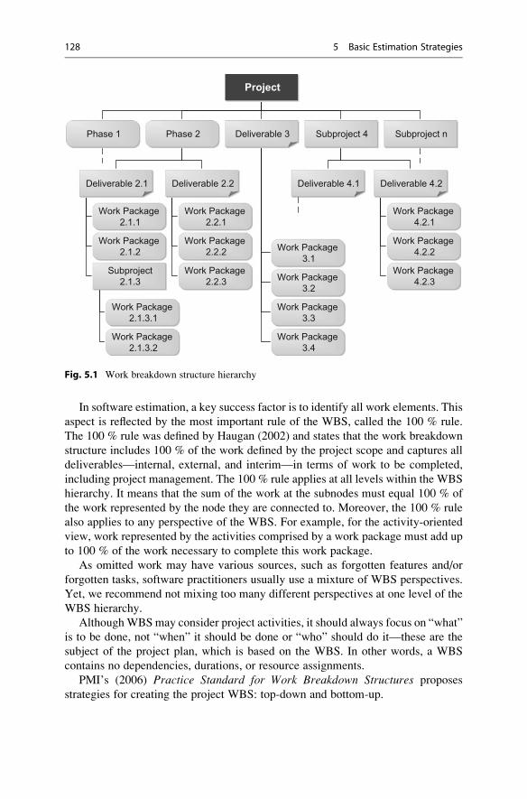
5.2.1 Work Breakdown Structure

The work breakdown structure (WBS) is a method for identifying work

components. It is widely used in the context of effort estimation and relies on

hierarchical decomposition of project elements. Figure 5.1 shows an example WBS

hierarchy. Three major perspectives of the WBS approach are applied in practice:

• Deliverable-oriented: It is a classical approach, defined by PMI (2013), in which

decomposition is structured by the physical or functional components of the

project. This approach uses major project deliverables as the first level of the

work breakdown structure.

• Activity-oriented: This approach focuses on the processes and activities in the

software project. It uses major life cycle phases as the first level of the work

breakdown structure.

• Organization-oriented: This approach focuses, similarly to the activity-oriented

one, on the project activities, but it groups them according to project organiza-

tional structure. This approach uses subprojects or components of the project as

the first level of the work breakdown structure. Subprojects can be identified

according to aspects of project organization as created subsystems, geographic

locations, involved departments or business units, etc. We may consider

employing organization-oriented WBS in the context of a distributed

development.

5.2 Bottom-Up Estimation Approach 127

In software estimation, a key success factor is to identify all work elements. This

aspect is reflected by the most important rule of the WBS, called the 100 % rule.

The 100 % rule was defined by Haugan (2002) and states that the work breakdown

structure includes 100 % of the work defined by the project scope and captures all

deliverables—internal, external, and interim—in terms of work to be completed,

including project management. The 100 % rule applies at all levels within the WBS

hierarchy. It means that the sum of the work at the subnodes must equal 100 % of

the work represented by the node they are connected to. Moreover, the 100 % rule

also applies to any perspective of the WBS. For example, for the activity-oriented

view, work represented by the activities comprised by a work package must add up

to 100 % of the work necessary to complete this work package.

As omitted work may have various sources, such as forgotten features and/or

forgotten tasks, software practitioners usually use a mixture of WBS perspectives.

Yet, we recommend not mixing too many different perspectives at one level of the

WBS hierarchy.

AlthoughWBSmay consider project activities, it should always focus on “what”

is to be done, not “when” it should be done or “who” should do it—these are the

subject of the project plan, which is based on the WBS. In other words, a WBS

contains no dependencies, durations, or resource assignments.

PMI’s (2006) Practice Standard for Work Breakdown Structures proposes

strategies for creating the project WBS: top-down and bottom-up.

Project

Subproject nPhase 1 Phase 2

Deliverable 4.1Deliverable 2.1 Deliverable 2.2

Work Package 2.2.1

Work Package 2.2.2

Work Package 2.1.1

Work Package 2.1.2

Work Package 2.2.3

Deliverable 3

Work Package 3.1

Work Package 3.4

Work Package 3.3

Work Package 3.2

Work Package 4.2.1

Work Package 4.2.3

Work Package 4.2.2

Deliverable 4.2

Work Package 2.1.3.1

Work Package 2.1.3.2

Subproject 4

Subproject2.1.3

Fig. 5.1 Work breakdown structure hierarchy


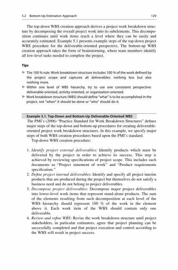
The top-down WBS creation approach derives a project work breakdown struc-

ture by decomposing the overall project work into its subelements. This decompo-

sition continues until work items reach a level where they can be easily and

accurately estimated. Example 5.1 presents example steps of the top-down project

WBS procedure for the deliverable-oriented perspective. The bottom-up WBS

creation approach takes the form of brainstorming, where team members identify

all low-level tasks needed to complete the project.

Tips

" The 100 % rule: Work breakdown structure includes 100 % of the work defined by

the project scope and captures all deliverables: nothing less but also

nothing more." Within one level of WBS hierarchy, try to use one consistent perspective:

deliverable-oriented, activity-oriented, or organization-oriented." Work breakdown structure (WBS) should define “what” is to be accomplished in the

project, not “when” it should be done or “who” should do it.

Example 5.1. Top-Down and Bottom-Up Deliverable-Oriented WBS

The PMI’s (2006) “Practice Standard for Work Breakdown Structures” defines

major steps of the top-down and bottom-up procedures for creating deliverable-

oriented project work breakdown structures. In this example, we specify major

steps of both WBS creation procedures based upon the PMI’s standard.

Top-down WBS creation procedure:

1. Identify project external deliverables: Identify products which must be

delivered by the project in order to achieve its success. This step is

achieved by reviewing specifications of project scope. This includes such

documents as “Project statement of work” and “Product requirements

specification.”

2. Define project internal deliverables: Identify and specify all project interim

products that are produced during the project but themselves do not satisfy a

business need and do not belong to project deliverables.

3. Decompose project deliverables: Decompose major project deliverables

into lower-level work items that represent stand-alone products. The sum

of the elements resulting from such decomposition at each level of the

WBS hierarchy should represent 100 % of the work in the element

above it. Each work item of the WBS should contain only one

deliverable.

4. Review and refine WBS: Revise the work breakdown structure until project

stakeholders, in particular estimators, agree that project planning can be

successfully completed and that project execution and control according to

the WBS will result in project success.


Bottom-up WBS creation procedure:

1. Identify all project deliverables: Identify all products or work packages

comprised by the project. For each work package or activity, exactly one

product that it delivers should be identified.

2. Group deliverables: Logically group related project deliverables or work

packages.

3. Aggregate deliverables: Synthesize identified groups of deliverables into the

next level in theWBS hierarchy. The sum of the elements at each level should

represent 100 % of the work below it, according to the 100 % rule.

4. Revise deliverables: Analyze the aggregated WBS element to ensure that you

have considered all of the work it encompasses.

5. Repeat steps 1 to 4: Repeat identifying, grouping, and aggregating project

deliverables until the WBS hierarchy is complete, that is, until a single top

node representing the project is reached. Ensure that the completed structure

comprises the complete project scope.

6. Review and refine WBS: Review the WBS with project stakeholders, and

refine it until they agree that the created WBS suffices for successful project

planning and completion.

For more details, refer to PMI’s (2006) “Practice Standard for Work Breakdown

Structures.” +

The top-down WBS creation approach is generally more logical and fits better

to a typical project planning scenario; thus, it is used in practice more often than

the bottom-up approach. The bottom-up approach tends to be rather chaotic,

consume much time, and often omit some of the low-level work activities.

Therefore, as a general rule, we recommend using top-down estimation in most

practical situations. The bottom-up WBS creation approach might be useful when

used in combination with a top-down approach for identifying redundant and

missing work items. Moreover, a bottom-up approach might be useful for revising

existing WBS, for instance, in the context of maintenance and evolution of

software systems.

Tip

" As a general rule, prefer the top-down approach for creating work breakdown

structure (WBS). Consider using bottom-up in combination with the top-down

approach for identifying redundant and omitted work items.

Table 5.1 summarizes situations, discussed by PMI (2006), when we should

consider top-down and bottom-up WBS development procedures.


Validating Outcomes of WBSOne way of validating WBS is to check its elements (work items) if they

fulfill the following requirements:

• Definable: Can be described and easily understood by project participants.• Manageable: A meaningful unit of work (responsibility and authority) can

be assigned to a responsible individual.

• Estimable: Effort and time required to complete the associated work can

be easily and reliably estimated.

• Independent: There is a minimum interface with or dependence on other

elements of the WBS (e.g., elements of WBS are assignable to a single

control account and clearly distinguishable from other work packages).

• Integrable: Can be integrated with other project work elements and with

higher-level cost estimates and schedules to include the entire project.

• Measurable: Can be used to measure progress (e.g., have start and com-

pletion dates and measurable interim milestones).

• Adaptable: Are sufficiently flexible, so the addition/elimination of work

scope can be readily accommodated in the WBS.

• Accountable: Accountability of each work package can be assigned to a

single responsible (human resource).

• Aligned/compatible: Can be easily aligned with the organizational and

accounting structures.

For a more comprehensive list of aspects to be considered when evaluating

the quality of a WBS, refer to PMI’s (2006) Practice Standard for Work

Breakdown Structures.

Table 5.1 When to use top-down and bottom-up WBS approaches

Top-down Bottom-up

Project manager and development management

team have little or no experience in developing

WBS. Top-down procedure allows for

progressive understanding and modeling of the

project scope

Project manager and development team have

large experience in creating WBS. Team

members can easily identify a project’s bottom-

up deliverables and follow the bottom-up WBS

procedure

The nature of the software products or services

is not well understood. Creating WBS jointly

with project stakeholders using the top-down

approach supports the achievement of common

understanding and consensus with respect to the

project’s nature and scope—especially when

they are initially unclear

The nature of the software products or services

is well understood. The project team has past

experiences with similar products and services,

and has a very good understanding of all interim

deliverables required for the project

(continued)


5.2.2 Method of Proportions

The so-called method of proportions is (after WBS) another popular instantiation of

the bottom-up estimation strategy. This method uses estimates or actual values from

one or more development phases of a new project as a basis for extrapolating the

total development effort. The extrapolation uses a percentage effort distribution

over the development phases observed in historical projects, which, at best, are

those that are the most similar to the new project.

Example 5.2. Bottom-Up Estimation Using the Method of Proportions

Let us assume the following situation. A project manager estimates software

development effort based on user requirements and needs to predict effort

required to maintain the developed software for an a priori assumed

operation time.

In the first step, the project manager identifies the most relevant

characteristics of the new software, especially those that are critical for mainte-

nance of the software. Next, he looks for already completed projects where

similar software has been developed and where the maintenance effort is already

known.

After analyzing already completed, historical projects, the project manager

selects the one most similar (analog) project and analyzes the distribution of

development and maintenance effort. He may also select more than one similar

project and use their actual efforts for deriving the estimate. Figure 5.2 illustrates

example effort distributions for historical and new projects. The project manager

analyzes the percentage distribution of the total life cycle effort among the

development and maintenance phases. Assuming that maintenance in the new

project will take the same percentage of total effort as in the historical project, he

extrapolates the maintenance effort of the new project based on its estimated

Table 5.1 (continued)

Top-down Bottom-up

The project life cycle is not clear or well known.

Top-down creation of WBS allows for

uncovering issues with respect to the software

development life cycle, especially in the case of

activity-oriented WBS

The project life cycle is clear and well known.

Software organization uses a well-defined

project life cycle, and all project members are

familiar with it. In such cases, the development

team can easily identify interim project

deliverables and use them to start bottom-up

WBS elaboration

No appropriate WBS templates are available.

Developing WBS from scratch is far easier in a

top-down manner, starting from the overall

project deliverable and then iteratively

determining its subelements

Appropriate WBS templates are available. The

software organization has already developed

work breakdown structures for similar projects

with similar products or services. These can be

easily reused and enhanced within a bottom-up

approach


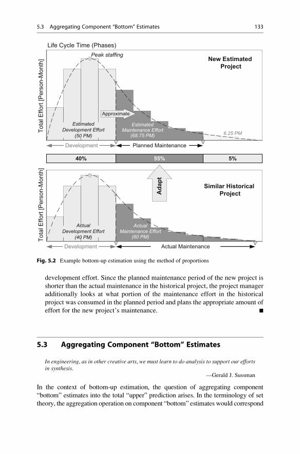
development effort. Since the planned maintenance period of the new project is

shorter than the actual maintenance in the historical project, the project manager

additionally looks at what portion of the maintenance effort in the historical

project was consumed in the planned period and plans the appropriate amount of

effort for the new project’s maintenance. +

5.3 Aggregating Component “Bottom” Estimates

In engineering, as in other creative arts, we must learn to do analysis to support our effortsin synthesis.

—Gerald J. Sussman

In the context of bottom-up estimation, the question of aggregating component

“bottom” estimates into the total “upper” prediction arises. In the terminology of set

theory, the aggregation operation on component “bottom” estimates would correspond

Peak staffing

EstimatedDevelopment Effort

(50 PM)

Development Planned Maintenance

Tota

l Effo

rt [P

erso

n-M

onth

] To

tal E

ffort

[Per

son-

Mon

th]

ActualDevelopment Effort

(40 PM)

Development Actual Maintenance

Estimated Maintenance Effort

(68.75 PM)

Similar Historical Project

New Estimated Project

Life Cycle Time (Phases)

Ada

pt40% 55% 5%

ActualMaintenance Effort

(60 PM)

Approximate

6.25 PM

Fig. 5.2 Example bottom-up estimation using the method of proportions

5.3 Aggregating Component “Bottom” Estimates 133

to the union (sum) operation on sets. A simple approach for synthesizing “bottom”

estimates can be by just summing them together. Yet, in practice, such simple and

“intuitive”methods may often lead to invalid results.Moreover, a number of questions

may arise such as, for instance, how to aggregate range estimates? In this section, we

discuss alternative approaches for aggregating multiple component estimates.

5.3.1 Aggregating Component Point Estimates

In the context of point estimation, the simple sum of component effort seems to be the

most reasonable choice; yet, it may lead to strange results. There are a few issues we

should not ignore before deciding on the particular approach for aggregating point

estimates.

One issue to consider is that improper decomposition of project work may result

in omitted and/or redundant activities and, in consequence, lead to under- or

overestimations (we discuss work decomposition in Sect. 5.2). If we know from

experience that we consequently tend to under- or overestimate, we should consider

this before summing up component estimates. Simple summation will also accu-

mulate our estimation bias—either toward under- or overestimates.

Yet, we might be lucky if we tend to approximately equally under- and overesti-

mate. In this case, mutual compensation of prediction error made on the level of

individual “bottom” estimates may lead to quite accurate total estimates—even

though component estimates were largely under- and overestimated. In statistics,

this phenomenon is related to the so-called law of large numbers. Its practical

consequence is that whereas the error of a single total prediction tends to be either

under- or overestimated, for multiple estimates some of themwill be under- and some

overestimated. In total, the errors of multiple component predictions tend to compen-

sate each other to some degree.

So far so good—we may think. Although imperfect decomposition of work

items may lead to estimation uncertainties, the law of large numbers works to our

advantage. Well, not quite, and as usual, the devil is in the details. There are a few

details that need consideration here. First, distribution of estimates is typically

consistently skewed toward either under- or overestimates. Moreover, the number

of component estimates is quite limited in real situations and restricts applicability

of the law of large numbers. Second, bottom-up estimation is typically applied in

the context of expert-based prediction where human experts tend to implicitly

(unconsciously) assign certain confidence levels to the point estimates they provide.

In this case, the probability of completing the whole project within the sum of

efforts estimated individually for all its component activities would be the joint

probability of each activity completing within its estimated effort. According to

probability theory, this would mean not summing up but multiplying probabilities

associated to individual estimates of each component activity.

Let us illustrate this issue with a simple example. We estimate the “most likely”

effort needed for completing ten project activities, which we identified in the

project work breakdown structure. “Most likely” means that each estimate is


50 % likely to come true; that is, we believe each activity will be completed within

its estimated effort with 50 % probability. In order to obtain the joint probability of

completing all the ten project activities—that is, completing the whole project—we

need to multiply probabilities associated to each individual “bottom” estimate. It

occurs that the probability of completing the project within estimated summary

effort would be merely 0.1 %.

A solution to the problem of summing up component point estimates is to

involve estimation uncertainty explicitly into the aggregation process. A simple

way of doing this is to collect minimum (“best-case”), most likely, and maximum

(“worst-case”) estimates for individual work items, aggregate them as probability

distributions, and then compute total expected value, for example, as a mean over

the resulting distribution. We discuss aggregating range and distribution estimates

in the next section (Sect. 5.3.2).

In conclusion, we should avoid simply summing point estimates, especially

when we suspect there are certain confidence levels associated with them. In

essence, we should actually avoid both point estimates and aggregating them by

simple summation. Whenever possible, we should include uncertainty into

estimates and combinations of such estimates.

Tip

" When applying bottom-up estimation, explicitly consider estimation uncertainty

and be aware of statistical subtleties of aggregating such predictions.

5.3.2 Aggregating Component Range Estimates

There are several approaches for aggregating uncertain component estimates. The

exact approach applies probability theory to formally aggregate probability density

functions of the variables represented by uncertain estimates. The approximateapproach includes applying simulation techniques. In the next paragraphs, we

present example aggregation methods for each of these two approaches.

Exact Approach: Sum of Random Variables

One way of aggregating estimates specified in terms of probability distributions is

to apply mechanisms provided by probability theory for summing random

variables. In probability theory, the distribution of the sum of two or more indepen-

dent, identically distributed random variables is represented by the so-called con-

volution of their individual distributions.

Many commonly used probability distributions have quite simple convolutions.

For example, the sum of two normal distributions X ~ (μx, σx2) and Y ~ (μY, σY

2) is a

normal distribution Z ~ (μx + μY, σx2 + σY

2), where μ and σ2 represent the distribu-tion mean and variance, respectively.


Constraints on Summing Multiple Random VariablesSums of multiple random variables require that

1. They have identical distributions, that is, all aggregated bottom estimates

are specified using the same probability distribution, and

2. They are independent, that is, the probability of a particular bottom effort

estimate does not depend on the probability of other estimates.

Although the independency of component estimates is a desired property

of bottom-up estimation, it may not always be provided. In the case of

dependent estimates, dedicated approaches proposed by probability theory

should be applied.

Exact discussion of these mechanisms is beyond the scope of our discussion and

can be found in a number of publications on probability theory, for example, in

Grinstead and Snell (2003).

Example 5.3 illustrates the practical application of the sum of random variables

for aggregating bottom estimates provided by human experts. In this example,

component estimates represent random variables with beta-PERT distribution.

Example 5.3. Program Evaluation and Review Technique (PERT)

Stutzke (2005) proposes applying the Program Evaluation and Review Technique(PERT) for aggregating bottom estimates provided by human experts. In PERT, the

estimator provides component (“bottom”) estimates in terms of three values: the

minimal, the maximal, and the most likely effort. It is assumed that these values are

unbiased and that the range between minimal and maximal estimates corresponds

to six standard deviation limits of the distribution. In other words, the effort

estimate is assumed to be a random variable with associated beta-PERT probability

distribution (as we discussed briefly in Sect. 4.4 and illustrated in Fig. 4.5).

As per probability theory, we assume mutual independence of component

estimates. Following this assumption, the convolution of individual distributions

is computed, in that total expected estimate (mean) is a sum of individual

expected estimates (5.1), and total variance is computed as a sum of variances

on individual estimates. Total standard deviation is then computed as a root

square from the total variance (5.2).

ExpectedTotal ¼Xni¼1

Expectedn, for n component estimates ð5:1Þ

where

Expectedi ¼Mini þ 4 MLi þMaxi

6



http://dx.doi.org/10.1007/978-3-319-03629-8_4#Fig5

σTotal ¼ffiffiffiffiffiffiffiffiffiffiffiffiXni¼1

σ2i

sð5:2Þ

where

σi ¼ Maxi �Mini

6

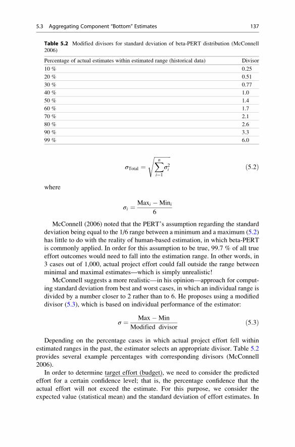
McConnell (2006) noted that the PERT’s assumption regarding the standard

deviation being equal to the 1/6 range between a minimum and a maximum (5.2)

has little to do with the reality of human-based estimation, in which beta-PERT

is commonly applied. In order for this assumption to be true, 99.7 % of all true

effort outcomes would need to fall into the estimation range. In other words, in

3 cases out of 1,000, actual project effort could fall outside the range between

minimal and maximal estimates—which is simply unrealistic!

McConnell suggests a more realistic—in his opinion—approach for comput-

ing standard deviation from best and worst cases, in which an individual range is

divided by a number closer to 2 rather than to 6. He proposes using a modified

divisor (5.3), which is based on individual performance of the estimator:

σ ¼ Max�Min

Modified divisorð5:3Þ

Depending on the percentage cases in which actual project effort fell within

estimated ranges in the past, the estimator selects an appropriate divisor. Table 5.2

provides several example percentages with corresponding divisors (McConnell

2006).

In order to determine target effort (budget), we need to consider the predicted

effort for a certain confidence level; that is, the percentage confidence that the

actual effort will not exceed the estimate. For this purpose, we consider the

expected value (statistical mean) and the standard deviation of effort estimates. In

Table 5.2 Modified divisors for standard deviation of beta-PERT distribution (McConnell

2006)

Percentage of actual estimates within estimated range (historical data) Divisor

10 % 0.25

20 % 0.51

30 % 0.77

40 % 1.0

50 % 1.4

60 % 1.7

70 % 2.1

80 % 2.6

90 % 3.3

99 % 6.0


order to simplify calculations, we take advantage of certain laws of probability

theory, in particular the central limit theorem, which states that the sum of many

independent distributions converges to a normal distribution as the number of

component distributions increases.

Assuming Normal Distribution: Exact ApproachIn practice, we do not make a significant error by assuming the total estimate

is normally distributed. On the one hand, the sum of independent distributions

converges to the normal curve very rapidly. Moreover, the error we make by

approximating normal distribution is small compared to the typical estima-

tion accuracy objectives, for example, �20 %.

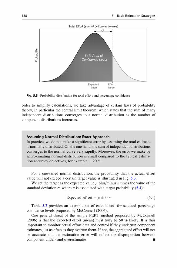
For a one-tailed normal distribution, the probability that the actual effort

value will not exceed a certain target value is illustrated in Fig. 5.3.

We set the target as the expected value μ plus/minus n times the value of the

standard deviation σ, where n is associated with target probability (5.4):

Expected effort ¼ μ� t � σ ð5:4ÞTable 5.3 provides an example set of calculations for selected percentage

confidence levels proposed by McConnell (2006).

One general threat of the simple PERT method proposed by McConnell

(2006) is that the expected effort (mean) must truly be 50 % likely. It is thus

important to monitor actual effort data and control if they underrun component

estimates just as often as they overrun them. If not, the aggregated effort will not

be accurate and the estimation error will reflect the disproportion between

component under- and overestimates. +

Total Effort (sum of bottom estimates)

Pro

babi

lity

Expected Effort

Effort Target

s

84% Area of Confidence Level

Fig. 5.3 Probability distribution for total effort and percentage confidence


Approximate Approach: Simulation

The exact method for aggregating uncertain estimates may involve complex math-

ematical formulas. Therefore, approximate approaches based on simulation

techniques have alternatively been proposed.

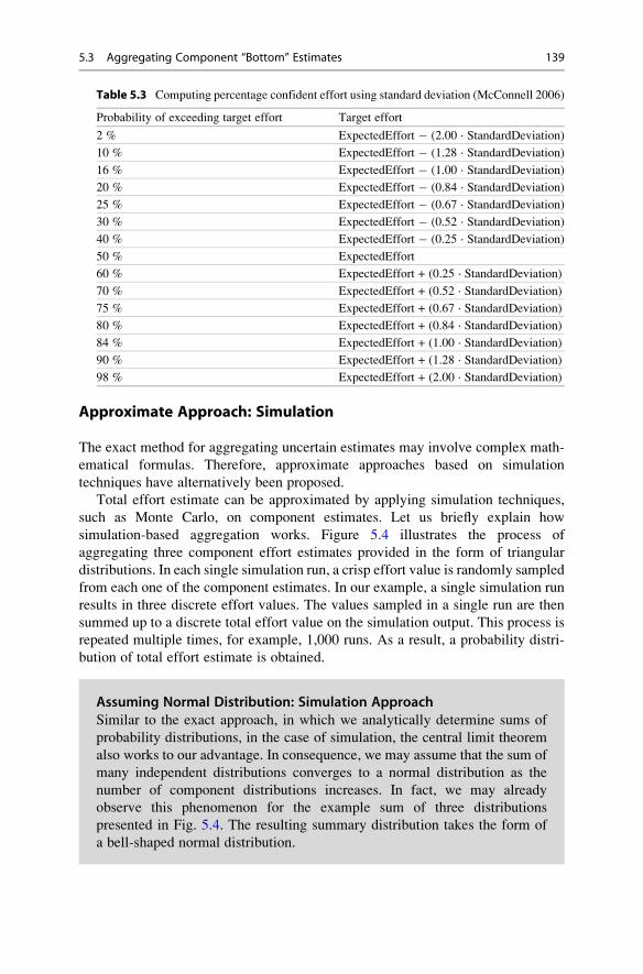
Total effort estimate can be approximated by applying simulation techniques,

such as Monte Carlo, on component estimates. Let us briefly explain how

simulation-based aggregation works. Figure 5.4 illustrates the process of

aggregating three component effort estimates provided in the form of triangular

distributions. In each single simulation run, a crisp effort value is randomly sampled

from each one of the component estimates. In our example, a single simulation run

results in three discrete effort values. The values sampled in a single run are then

summed up to a discrete total effort value on the simulation output. This process is

repeated multiple times, for example, 1,000 runs. As a result, a probability distri-

bution of total effort estimate is obtained.

Assuming Normal Distribution: Simulation ApproachSimilar to the exact approach, in which we analytically determine sums of

probability distributions, in the case of simulation, the central limit theorem

also works to our advantage. In consequence, we may assume that the sum of

many independent distributions converges to a normal distribution as the

number of component distributions increases. In fact, we may already

observe this phenomenon for the example sum of three distributions

presented in Fig. 5.4. The resulting summary distribution takes the form of

a bell-shaped normal distribution.

Table 5.3 Computing percentage confident effort using standard deviation (McConnell 2006)

Probability of exceeding target effort Target effort

2 % ExpectedEffort � (2.00 · StandardDeviation)







50 % ExpectedEffort

60 % ExpectedEffort + (0.25 · StandardDeviation)








An example estimationmethod that actually uses simulation for integratingmultiple

uncertain bottom estimates was proposed by Elkjaer (2000) in the context of expert-

based estimation. His method, called Stochastic Budgeting Simulation, employs ran-

dom sampling to combine the effort of individual effort items, such as work products or

development activities, specified by experts in terms of triangular distributions.

5.4 Selecting Appropriate Estimation Strategy

An intelligent plan is the first step to success. The man who plans knows where he is going,knows what progress he is making and has a pretty good idea when he will arrive.

—Basil S. Walsh

Depending on the particular project application context, both top-down and bottom-

up approaches for project effort estimation have various advantages and

disadvantages.

Estimation Strategy and Estimation MethodIn the related literature, top-down and bottom-up estimations are often

referred to as estimation methods. In our opinion, top-down and bottom-up

approaches refer more to an overall estimation strategy rather than to a

particular estimation method. In principle, any estimation method, such as

regression analysis or expert judgment, can be used within any of these two

strategies; although not every estimation method is equally adequate and easy

to apply within each of these two strategies.

1 3 5 7 9 11 13 150.0

0.2

0.1

0.3

0.4

0.5

0.6

0.7

0.8

0.9

1.0

Triangular Distribution B

1 2 3 4 5 60.0

0.2

0.1

0.3

0.4

0.5

0.6

0.7

0.8

0.9

1.0

0.0

0.2

0.1

0.3

0.4

0.5

0.6

0.7

0.8

0.9

1.0

0.0

0.2

0.1

0.3

0.4

0.5

0.6

0.7

0.8

0.9

1.0Triangular

Distribution ATriangular

Distribution C

1 2 3 4 5 61 2 3 4 5 6

Union of Distributions

A

B

C

Sum samplesfrom all inputs

Single simulation run

Fig. 5.4 Aggregating component estimates using simulation


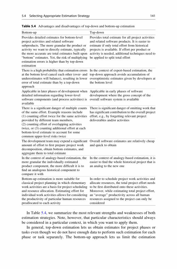
In Table 5.4, we summarize the most relevant strengths and weaknesses of both

estimation strategies. Note, however, that particular characteristics should always

be considered in a particular context, in which you want to apply them.

In general, top-down estimation lets us obtain estimates for project phases or

tasks even though we do not have enough data to perform such estimation for each

phase or task separately. The bottom-up approach lets us limit the estimation

Table 5.4 Advantages and disadvantages of top-down and bottom-up estimation

Bottom-up Top-down

Provides detailed estimates for bottom-level

project activities and related software

subproducts. The more granular the product or

activity we want to directly estimate, typically

the more accurate are total estimates built upon

“bottom” estimates. Yet, the risk of multiplying

estimation errors is higher than by top-down

estimation

Provides total estimate for all project activities

and related software products. It is easier to

estimate if only total effort from historical

projects is available. If effort per product or

activity is needed, additional techniques need to

be applied to split total effort

There is a high probability that estimation errors

at the bottom level cancel each other (over- and

underestimates will balance), resulting in lower

error of total estimate than by a top-down

approach

In the context of expert-based estimation, the

top-down approach avoids accumulation of

overoptimistic estimates given by developers at

the bottom level

Applicable in later phases of development when

detailed information regarding lower-level

software components (and process activities) is

available

Applicable in early phases of software

development where the gross concept of the

overall software system is available

There is a significant danger of multiple counts

of the same effort. Example reasons include

(1) counting effort twice for the same activities

provided by different team members,

(2) counting effort of overlapping activities

twice, or (3) counting additional effort at each

bottom-level estimate to account for some

common upper-level risks twice

There is significant danger of omitting work that

has significant contribution to the overall project

effort, e.g., by forgetting relevant project

deliverables and/or activities

The development team may expend a significant

amount of effort to first prepare project work

decomposition, obtain bottom estimates, and

aggregate them to total estimate

Overall software estimates are relatively cheap

and quick to obtain

In the context of analogy-based estimation, the

more granular the individually estimated

product component, the more difficult it is to

find an analogous historical component to

compare it with

In the context of analogy-based estimation, it is

easier to find the whole historical project that is

an analog to the new one

Bottom-up estimation is more suitable for

classical project planning in which elementary

work activities are a basis for project scheduling

and resource allocation. Estimating effort for

individual work activities allows for considering

the productivity of particular human resources

preallocated to each activity

In order to schedule project work activities and

allocate resources, the total project effort needs

to be first distributed onto these activities.

Moreover, while estimating total project effort,

an “average” productivity across all human

resources assigned to the project can only be

considered

5.4 Selecting Appropriate Estimation Strategy 141

abstraction level. It is especially useful in the case of expert-based estimation,

where it is easier for experts to embrace and estimate smaller pieces of project

work. Moreover, the increased level of detail during estimation—for instance, by

breaking down software products and processes—implies higher transparency of

estimates.

In practice, there is a good chance that the bottom estimates would be mixed

below and above the actual effort. As a consequence, estimation errors at the

bottom level will cancel each other out, resulting in smaller estimation error than

if a top-down approach were used. This phenomenon is related to the mathematical

law of large numbers.1 However, the more granular the individual estimates, the

more time-consuming the overall estimation process becomes.

In industrial practice, a top-down strategy usually provides reasonably accurate

estimates at relatively low overhead and without too much technical expertise.

Although bottom-up estimation usually provides more accurate estimates, it

requires the estimators involved to have expertise regarding the bottom activities

and related product components that they estimate directly.

In principle, applying bottom-up estimation pays off when the decomposed tasks

can be estimated more accurately than the whole task. For instance, a bottom-up

strategy proved to provide better results when applied to high-uncertainty or

complex estimation tasks, which are usually underestimated when considered as a

whole. Furthermore, it is often easy to forget activities and/or underestimate the

degree of unexpected events, which leads to underestimation of total effort.

However, from the mathematical point of view (law of large numbers mentioned),

dividing the project into smaller work packages provides better data for estimation

and reduces overall estimation error.

Experiences presented by Jørgensen (2004b) suggest that in the context of

expert-based estimation, software companies should apply a bottom-up strategy

unless the estimators have experience from, or access to, very similar projects. In

the context of estimation based on human judgment, typical threats of individual

and group estimation should be considered. Refer to Sect. 6.4 for an overview of the

strengths and weaknesses of estimation based on human judgment.

Tip

" Developers typically tend to be optimistic in their individual estimates (underesti-

mate). As a project manager, do not add more optimism by reducing the

developers’ estimates.

1 In statistics, the law of large numbers says that the average of a large number of independent

measurements of a random quantity tends toward the theoretical average of that quantity. In the

case of effort estimation, estimation error is assumed to be normally distributed around zero. The

consequence of the law of large numbers would thus be that for a large number of estimates, the

overall estimation error tends toward zero.



In both strategies, the ability of the software estimation method and/or model to

transfer estimation experience from less similar projects leads to equally poor

estimates. In other words, lack of quantitative experiences from already completed

projects leads to poor predictions independent of whether the data-driven method

estimates the whole project or its components.

In summary, although the bottom-up approach intuitively seems to provide

better data for estimation, the selection of the proper strategy depends on the task

characteristics and the level of the estimators’ experience. In principle, one should

prefer top-down estimation in the early (conceptual) phases of a project and switch

to bottom-up estimation where specific development tasks and assignments are

known.

Tip

" Prefer top-down estimation in the early (conceptual) phases of a project and

switch to bottom-up estimation where specific development tasks and assign-

ments are known. Consider using top-down estimation strategy for cross-checking

bottom-up estimates (and vice versa).

Finally, whenever accurate estimates are relatively important and estimation

costs are relatively low, compared to overall project effort, we recommend using

both estimation strategies for validation purposes.

5.5 Using Multiple Alternative Estimation Methods

In combining the results of these two methods, one can obtain a result whose probability oferror will more rapidly decrease.

—Pierre Laplace

A number of effort estimation methods have been proposed over the recent decades.

Yet, no “silver-bullet” method has been proposed so far, and it is actually hard to

imagine that such a “one-size-fits-all” estimation method will ever be created. Each

and every estimation method has its own specific strengths and limitations, which

depend on the particular situation in which the method is used. The most important

consequence of this fact is that a combination of different estimation approaches

may substantially improve the reliability of estimates.

In practice, there are two ways of implementing the idea of combining multiple

estimation methods or paradigms:

• Hybrid estimation method: In this approach, elements of different estimation

paradigms, for example, expert-based and data-driven estimation, are integrated

within a hybrid estimation method. Hybrid estimation may use alternative

information sources and combine multiple elementary techniques into a single

estimation method, which typically represents alternative estimation paradigms.

We discuss hybrid estimation methods in Sect. 6.5.

5.5 Using Multiple Alternative Estimation Methods 143


• Multiple alternative methods: In this approach, multiple alternative methods are

applied independently to estimate the same work, and their outcome estimates

are combined into a final estimate. Similar to hybrid estimation, multiple

alternative methods should preferably represent different estimation paradigms

and be based on alternative, yet complementary, information sources.

A major benefit of using multiple estimation methods is the possibility of

validating alternative estimates against each other. In the case of significantly

inconsistent estimates, we may investigate sources of potential discrepancies

between alternative estimates, improve them if possible, and combine them when

they start to converge.

Tip

" In order to validate and improve prediction accuracy, combine estimates provided

by several methods that represent substantially different estimation paradigms

and use different sources of information.

A major drawback of using alternative estimation methods is the large overhead

required to perform multiple estimations with different methods. We should there-

fore consider using multiple estimation methods and combining alternative

estimates only when

• It is very important to avoid large estimation errors. For example, we know that

the cost of potential prediction error is much higher than the cost of applying

multiple estimation methods.

• We are uncertain about the situation in which the estimation method is to be

applied. For example, the project environment has not been precisely specified

yet, and estimation inputs and constraints are not clear.

• We are uncertain about which forecasting method is more accurate. Since, in

most cases, we are uncertain about which method is the most accurate, it is

always good to consider the use of several methods.

• There is more than one reasonable estimation method available. In practice, we

recommend using two alternative methods that differ substantially with respect

to the estimation paradigm and to use different sources of information.

5.6 Combining Alternative Estimates

Based on the extensive evidence in favour of combining estimates the question should notbe whether we should combine or not, but how?

—Magne Jørgensen

When using multiple estimation methods, we must face the issue of combining

multiple effort estimates that these methods provide into a single final prediction. In

contrast to combining component estimates in the context of bottom-up estimation


(Sect. 5.3) where we summed up partial estimates, in the context of applying

multiple estimation methods, we are interested in finding a consensus between

multiple estimates. Using the terminology of set theory, combining multiple alter-

native estimates would correspond to the intersection operation.

5.6.1 Combining Largely Inconsistent Estimates

In practice, uncritically combining estimates that differ widely may lead to signifi-

cant errors. We may consider using sophisticated methods for avoiding the impact

of outlier estimates. Yet, outlier analysis requires several values, whereas in

practice, we will typically have two or three alternative values. Moreover, in the

case of outlier analysis, it is not clear if estimates identified as outliers are not the

correct ones that should not be excluded from consideration. The simple “majority”

rule does not apply to software effort estimation. We need to consider if each

individual estimate may be right and then decide on the combined estimate.

Therefore, before combining estimates, one should investigate possible sources of

discrepancy between outputs of alternative estimation approaches.

At best, estimation should be repeated after potential sources of inconsistencies

have been clarified. This process can be repeated until estimates converge and the

observed discrepancy is not greater than 5 %. Then, an appropriate aggregation

approach should be selected and applied to come up with final effort estimates.

In an extreme case, excluding an estimation method that provides outlier

estimates should be considered if the sources of deviation are clear and nothing

can be done to improve the convergence of estimates. Yet, this option should be

considered very carefully as it may occur that extreme estimates were the most

exact ones.

Tip

" If estimates provided by alternative methods differ widely, then investigate the

reasons for this discrepancy, before combining the estimates. Continue

investigating the reasons for discrepancy between estimates provided by alterna-

tive methods until the estimates converge to within about 5 %. Exclude individual

estimation methods from the prediction process if necessary, for example, if they

clearly provide incorrect estimates and nothing can be done to improve them.

Combine alternative estimates when they start to converge.

5.6.2 Combining Alternative Point Estimates

Statistical Techniques

Common statistical means for combining multiple point estimates include taking a

simple mean or mode value over a number of individual estimates. Yet, individual

5.6 Combining Alternative Estimates 145

forecasts may be burdened by large errors, for example, due to miscalculations,

errors in data, or misunderstanding of estimation scope and context. In such cases, it

is useful to exclude the extremely high and extremely low predictions from the

analysis.

Example statistical means that deal with extreme values—so-called outliers—

include trimmed means or medians. A less radical approach for handling deviations

between individual estimates would be by applying a weighted average, where

weights reflect the believed credibility of each estimate. In the case of expert-based

estimation, these weights may reflect the experts’ level of competence regarding the

estimated tasks. When combining predictions provided by data-driven and expert-

based methods, higher weight may be assigned to data-driven estimates if a large set

of high-quality data is available, or to expert-based methods, otherwise—especially

when highly experienced estimators are involved. We recommend, after Armstrong

(2001), using equal weights unless strong evidence or belief exists to support

unequal weighting.

Tip

" When combining multiple estimates by means of weighted average, use equal

weights unless you have strong evidence to support unequal weighting of alter-

native estimates.

Expert Group Consensus

As an alternative to a statistical approach, we may combine multiple alternative

effort estimates in a group consensus session. In this approach, alternative estimates

are discussed within a group of human experts, where each expert typically

represents one individual estimate. As a result of discussion, experts come up

with a consensus regarding the final estimate.

Although it can theoretically be applied for any estimation method, the group

consensus approach is typically applied in the context of estimation based on

human judgment (Sect. 6.4.2). In this context, alternative estimates are provided

by individual human experts and then combined in the group discussion.

A group debate might have the form of an unstructured meeting or follow a

systematic process, such as one defined by existing group consensus techniques.

Examples of the structured group discussion techniques are Wideband Delphi(Chap. 12) or, created in the context of agile development, Planning Poker(Chap. 13).

The performance of individual group consensus methods typically varies

depending on the characteristics of the group, such as motivation of involved

experts, their social relations, and communication structure in a group. A common

threat is human and situational bias of a group discussion. We address these

problems in Sect. 6.4.3, where we discuss effort estimation methods based on

group discussion.



http://dx.doi.org/10.1007/978-3-319-03629-8_12

http://dx.doi.org/10.1007/978-3-319-03629-8_13


Also, characteristics of tasks estimated have an impact on the performance of

different group discussion techniques. For example, Haugen (2006) observed that

for tasks that experts were familiar with, the planning poker technique delivered

more accurate estimates than unstructured combination—the opposite was found

for tasks with which experts were unfamiliar.

In the context of expert-based effort estimation, statistical combination of

individual experts’ estimates was, surprisingly, found less effective than combining

them in a group discussion process. Moløkken-Østvold et al. (2004, 2008) observed

that group estimates made after an unstructured discussion were more realistic than

individual estimates derived prior to the group discussion and combined by statisti-

cal means. It is the group discussion that seems to be the key factor reducing the

overoptimism in individual estimates. Thus, even taking a simple average, that is, a

statistical mean, of individual estimates should often work well under the condition

that they were provided after a group discussion. We generally advise conducting

an unstructured discussion before experts provide their individual estimates and

before we combine these estimates.

Tip

" When considering multiple expert estimates, perform a group discussion session

before combining individual estimates—independent of the approach used to

combine alternative estimates.

5.6.3 Combining Alternative Range Estimates

Statistical Techniques

A simple statistical approach for combining alternative range estimates might be by

taking an average, that is, a statistical mean, of the individual minimum and maxi-

mum predictions. This approach seems to work well in many practical situations. For

example, Armstrong (2001) observed in a number of empirical studies that

predictions based on the simple mean across all individual predictions were on

average 12.5%more accurate than the mean of a single randomly selected prediction.

Yet, combining estimates by means of a simple average has been observed

ineffective in the context of estimates based on human judgment, where prediction

intervals tend to be too narrow and not to correspond to the confidence level

believed by the experts. For example, experts believed to provide estimates of

90 % confidence, whereas the actual confidence level represented by intervals they

provided was about 70 %. In such situations, applying a simple average over

individual minimums and maximums does not improve correspondence between

believed and actual confidence levels, that is, it does not deal with overoptimism of

the individual estimates.

Jørgensen and Moløkken (2002) observed that in the context of expert-based

estimation, taking the maximum and minimum of individual maximum and mini-

mum predictions is much more effective than taking averages. In this approach,


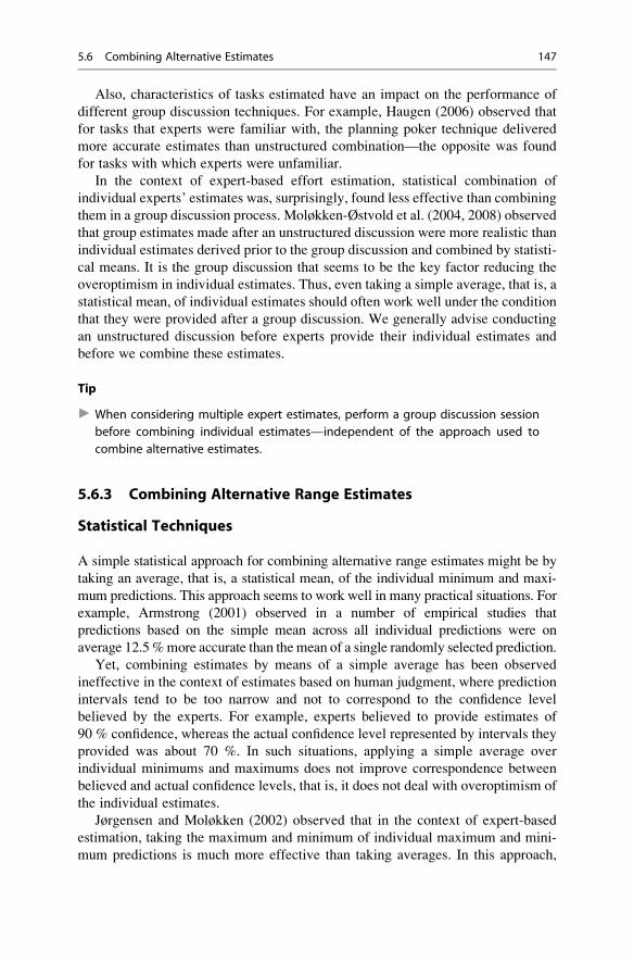
overoptimism of individual estimates is reduced by taking the widest interval over

all estimates. Figure 5.5 illustrates both average and min-max approaches for

combining alternative expert-based estimates. Note that in both cases, most likely

estimates are combined by way of simple statistical mean.

Expert Group Consensus

Similarly to combining point estimates, a group consensus approach seems to be

again a more effective way of synthesizing expert estimates than “automatic” statis-

tical approaches. In a group consensus approach, final estimates are agreed upon in a

group discussion. Although group consensus can be applied to combine any

estimates, it is typically applied in the context of expert-based estimation; that is,

for synthesizing alternative estimates provided by human experts. A group debate

might have the form of an unstructured meeting or follow a systematic process

defined by one of the existing group consensus techniques such asWideband Delphior Planning Poker. We present these methods in Chaps. 12 and 13, respectively.

Simulation Techniques

Similar to combining multiple component estimates in the context of bottom-

up estimation (Sect. 5.3), alternative estimates provided by different prediction

Interval Estimate A

1 2 3 4 5 60.0

0.2

0.1

0.3

0.4

0.5

0.6

0.7

0.8

0.9

1.0

0.0

0.2

0.1

0.3

0.4

0.5

0.6

0.7

0.8

0.9

1.0Interval

Estimate B

1 7 82 3 4 5 6 7 8

Combined Interval Estimate

1 3 5 60.0

0.2

0.1

0.3

0.4

0.5

0.6

0.7

0.8

0.9

1.0

0.0

0.2

0.1

0.3

0.4

0.5

0.6

0.7

0.8

0.9

1.0

1 85 7 8

Combined Interval Estimate

Avg(2, 3)

Min (2, 3) Max (5, 7)Avg (4, 4)

Interval width = (Max – Min) / MostLikelyEstimate (actual 90% confidence interval)

2 3 Avg(4, 4)

Avg(5, 7)

Expert estimate (believed 90% confidence interval)

Interval width = 0.75 Interval width = 1.00

Interval width = 0.86 Interval width = 1.25

Min-MaxAvg(Mean)

Fig. 5.5 Combining expert estimates using the “average” and “min–max” approaches


http://dx.doi.org/10.1007/978-3-319-03629-8_12

http://dx.doi.org/10.1007/978-3-319-03629-8_13

methods can also be combined using simulation approaches. However, other

than in the case of bottom-up estimation, we are not looking for a sum of

partial estimates but for their consensus, that is, their intersection in set

terminology.

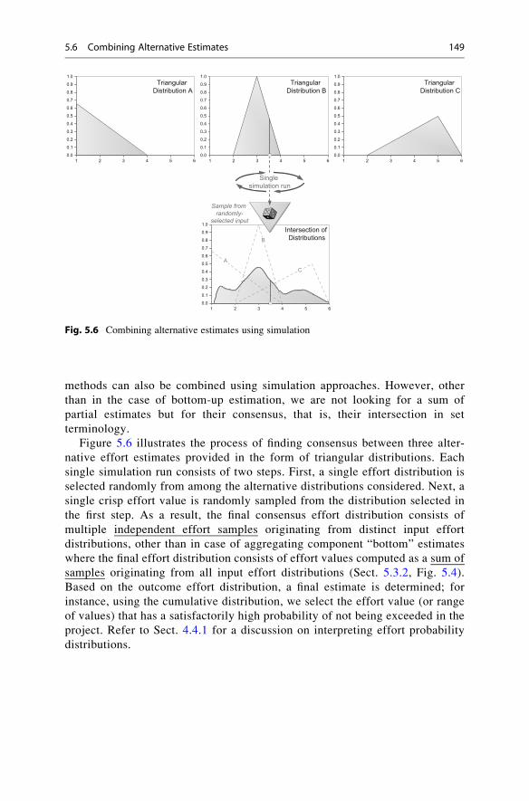
Figure 5.6 illustrates the process of finding consensus between three alter-

native effort estimates provided in the form of triangular distributions. Each

single simulation run consists of two steps. First, a single effort distribution is

selected randomly from among the alternative distributions considered. Next, a

single crisp effort value is randomly sampled from the distribution selected in

the first step. As a result, the final consensus effort distribution consists of

multiple independent effort samples originating from distinct input effort

distributions, other than in case of aggregating component “bottom” estimates

where the final effort distribution consists of effort values computed as a sum of

samples originating from all input effort distributions (Sect. 5.3.2, Fig. 5.4).

Based on the outcome effort distribution, a final estimate is determined; for

instance, using the cumulative distribution, we select the effort value (or range

of values) that has a satisfactorily high probability of not being exceeded in the

project. Refer to Sect. 4.4.1 for a discussion on interpreting effort probability

distributions.

Triangular Distribution B

1 2 3 4 5 60.0

0.2

0.1

0.3

0.4

0.5

0.6

0.7

0.8

0.9

1.0

0.0

0.2

0.1

0.3

0.4

0.5

0.6

0.7

0.8

0.9

1.0

0.0

0.2

0.1

0.3

0.4

0.5

0.6

0.7

0.8

0.9

1.0Triangular

Distribution ATriangular

Distribution C

1 2 3 4 5 61 2 3 4 5 6

Sample from randomly-

selected input

0.0

0.2

0.1

0.3

0.4

0.5

0.6

0.7

0.8

0.9

1.0

1 2 3 4 5 6

Single simulation run

Intersection of Distributions

A

B

C

Fig. 5.6 Combining alternative estimates using simulation



Determining Sampling LikelihoodWhile the probability of sampling particular crisp effort values from an input

distribution is determined by the distribution shape, the probability of

selecting the individual input distribution needs to be determined manually

up front. In a simple case, all inputs are assigned equal likelihood of being

picked up, that is, the selection follows according to a uniform discrete

probability distribution.

Yet, we may want to prefer particular input estimates over others and, thus,

to perform selection according to another schema represented by a specific

discrete probability distribution. For example, when finding consensus

between predictions provided by human experts and data-driven algorithmic

methods, we might prefer expert estimates because of low reliability of

quantitative data on which the data-driven predictions were based. And vice

versa, we might prefer data-driven estimates because they were based on

large sets of reliable data, whereas human estimates have little domain and

prediction experience.

Further Reading

• R.D. Stutzke (2005), Estimating Software-Intensive Systems: Projects, Products,and Processes, Addison-Wesley Professional.

In Chaps. 11 and 12 of his book, the author discusses bottom-up and top-down

estimation strategies, respectively. Example techniques for implementing both

estimation strategies are described. The author also discusses threats in making

effort-time trade-offs and schedule compression.

• Project Management Institute (2006), Practice Standard for Works BreakdownStructures. 2nd Edition. Project Management Institute, Inc. Pennsylvania, USA.

The practice standard provides a summary of best practices for defining work

breakdown structures. It provides an overview of the basic WBS process, criteria

for evaluating the quality of WBS, and typical considerations needed when

defining WBS. Finally, the standard provides a number of example work break-

down structures from various domains, including software development and

process improvement.

• R.T. Futrell, D.F. Shafer, and L. I. Shafer (2002), Quality Software ProjectManagement, Prentice Hall.

In their book, the authors discuss approaches for creating project work

breakdown structures and identifying project activities in the context of project

management. In Chap. 8, they present top-down and bottom-up strategies for

creating project-oriented WBS and show different WBS approaches that


implement these strategies. In Chap. 9, the authors show how to populate a WBS

to identify project activities and tasks relevant for effective project planning.

• IEEE Std 1074 (2006), IEEE Standard for Developing a Software Project LifeCycle Process, New York, NY, USA. IEEE Computer Society.

This standard provides a process for creating a process for governing software

development and maintenance. It lists common software development life cycle

phases, activities, and tasks. The standard does not imply or presume any

specific life cycle model.

• ISO/IEC 12207 (2008), International standard for Systems and SoftwareEngineering - Software Life Cycle Processes, International Organization for

Standardization and International Electrotechnical Commission (ISO/IEC), and

IEEE Computer Society.

Similar to the IEEE 1074 standard, this international standard aims at

specifying a framework for software life cycle processes. Yet, it comprises a

wider range of activities regarding life cycle of software/system product and

services. It spans from acquisition, through supply and development, to opera-

tion, maintenance, and disposal. Similar to IEEE 1074, this standard also does

not prescribe any particular life cycle model within which proposed phases and

activities would be sequenced.

• M. Jørgensen (2004), “Top-down and bottom-up expert estimation of software

development effort.” Information and Software Technology, vol. 46, no. 1,pp. 3–16.

The author investigates strengths and weaknesses of top-down and bottom-up

strategies in the context of expert-based effort estimation. In his industrial study,

the author asked seven teams of estimators to predict effort for two software

projects, where one project was to be estimated using a top-down strategy and

the other using a bottom-up strategy. In the conclusion, the author suggests

applying a bottom-up strategy unless estimators have experience from, or access

to, very similar historical projects.

• S. Fraser, B.W. Boehm, H. Erdogmus, M. Jørgensen, S. Rifkin, and M.A. Ross

(2009), “The Role of Judgment in Software Estimation,” Panel of the 31stInternational Conference on Software Engineering, Vancouver, Canada, IEEEComputer Society.

This short article documents a panel discussion regarding the role of expert

judgment and data analysis in software effort estimation. Panelists underline the

thesis that “there is nothing like judgment-free estimation” but also stress the

importance of quantitative historical information for software estimation.

• M. Jørgensen (2007), “Forecasting of software development work effort: Evi-

dence on expert judgment and formal models,” International Journal ofForecasting, vol. 23, no. 3, pp. 449–462.

Further Reading 151

This article provides a comprehensive review of published evidence on the

use of expert judgment, formal methods, and hybrid methods for the purpose of

software project effort estimation. The final conclusion is that combining model-

and expert-based approaches works principally better than either one alone.

• M. Jørgensen (2004), “A Review of Studies on Expert Estimation of Software

Development Effort,” Journal of Systems and Software, vol. 70, no. 1–2,

pp. 37–60.

In Sect. 5.2 of his article, the author provides an overview of various

approaches for combining multiple estimates provided by human experts. In

addition, he discusses typical factors on which benefits of combining multiple

expert estimates depend.

• M. Jørgensen and K. J. Moløkken (2002), “Combination of software develop-

ment effort prediction intervals: why, when and how?” Proceedings of the 14thInternational Conference on Software engineering and knowledge Engineering,Ischia, Italy, pp. 425–428.

The authors investigate an empirical study of three strategies for combining

multiple, interval estimates: (1) average of the individual minimum and maxi-

mum estimates, (2) maximum and minimum of the individual maximum and

minimum estimates, and (3) group discussion of estimation intervals. Results of

the study suggest that a combination of prediction intervals based on group

discussion provides better estimates than “mechanical” combinations. Yet, the

authors warn that there is no generally best strategy for combining prediction

intervals.


http://www.springer.com/978-3-319-03628-1

download sample pages 5 pdf

Documents