download-manuals-surface water-software-48appliedstatistics

World Bank & Government of The Netherlands funded

Training module # WQ - 48

Applied Statistics

New Delhi, September 2000

CSMRS Building, 4th Floor, Olof Palme Marg, Hauz Khas,New Delhi – 11 00 16 IndiaTel: 68 61 681 / 84 Fax: (+ 91 11) 68 61 685E-Mail: [email protected]

DHV Consultants BV & DELFT HYDRAULICS

withHALCROW, TAHAL, CES, ORG & JPS

HP Training Module File: “ 48 Applied Statistics.doc” Version: September 2000 Page 1

Table of contents

Page

1. Module context 2

2. Module profile 3

3. Session plan 4

4. Overhead/flipchart master 5

5. Evaluation sheets 21

6. Handout 23

7. Additional handout 30

8. Main text 32


1. Module context

This module discusses statistical procedures, which are commonly used by chemists toevaluate the precision and accuracy of results of analyses. Prior training in ‘Basic Statistic’,module no. 47, or equivalent is necessary to complete this module satisfactorily.

While designing a training course, the relationship between this module and the others,would be maintained by keeping them close together in the syllabus and place them in alogical sequence. The actual selection of the topics and the depth of training would, ofcourse, depend on the training needs of the participants, i.e. their knowledge level and skillsperformance upon the start of the course.


2. Module profile

Title : Applied Statistics

Target group : HIS function(s): Q2, Q3, Q5, Q6

Duration : one session of 90 min

Objectives : After the training the participants will be able to:• Apply common statistical tests for evaluation of the precision of

data

Key concepts : • confidence interval• regression analyses

Training methods : Lecture, exercises, OHS

Training toolsrequired

: Board, flipchart

Handouts : As provided in this module

Further readingand references

: • ‘Analytical Chemistry’, Douglas A. Skoog and Donald M. West,Saunders College Publishing, 1986 (Chapter 3)

• ‘Statistical Procedures for analysis of Environmenrtal monitoringData and Risk Assessment’, Edward A. Mc Bean and Frank A.Rovers, Prentice Hall, 1998.


3. Session plan

No Activities Time Tools1 Preparations

2 Introduction:• Need for statistical procedures• Scope of the module

10 min OHS

3 Confidence interval• Definition• Significance of standard deviation and its correct estimation• When population SD is known• When population SD is not known

30 min OHS

4 Rejection of Data• Caution in rejection• Procedures

20 min OHS

5 Regression analysis 20 min OHS

6 Wrap up 10 min


4. Overhead/flipchart masterOHS format guidelines

Type of text Style SettingHeadings: OHS-Title Arial 30-36, with bottom border line (not:

underline)

Text: OHS-lev1OHS-lev2

Arial 24-26, maximum two levels

Case: Sentence case. Avoid full text in UPPERCASE.

Italics: Use occasionally and in a consistent way

Listings: OHS-lev1OHS-lev1-Numbered

Big bullets.Numbers for definite series of steps. Avoidroman numbers and letters.

Colours: None, as these get lost in photocopying andsome colours do not reproduce at all.

Formulas/Equations

OHS-Equation Use of a table will ease horizontal alignmentover more lines (columns)Use equation editor for advanced formattingonly


Applied Statistics

• Confidence intervals

• Number of replicate observations

• Rejection of data

• Regression analysis


Confidence Intervals (1)

• Population mean µ is always unknown

• Sample mean x

- Only for large number of replicate x → µ

• Estimation of limits for µ from x

(x – a) < µ < (x + a)

• Value of a depend

- confidence level (probability of occurrence)

- standard deviation

- difference between limits is the interval


Confidence Intervals

Figure 1. Normal distribution curve and areas under curve for different distances



• When s is good estimate of σ

- for single observation, (x - zσ) < µ < (x - zσ)

Confidence level 50 90 95 99 99.7

Z 0.67 1.64 1.96 2.58 3

- as z or interval increases confidence level also increases


Example (1)

• Mercury concentration in fish was determined as 1.8 µg/kg.Calculate limits for µ for 95% confidence level if σ = 0.1 µg/kg

- For 95% confidence level z = 1.96

- Limits for mean

1.8 – 1.96 x 0.1 < µ < 1.8 + 1.96 x 0.1

1.6 < µ < 2.0

• What are the limits for 99.7% confidence level?



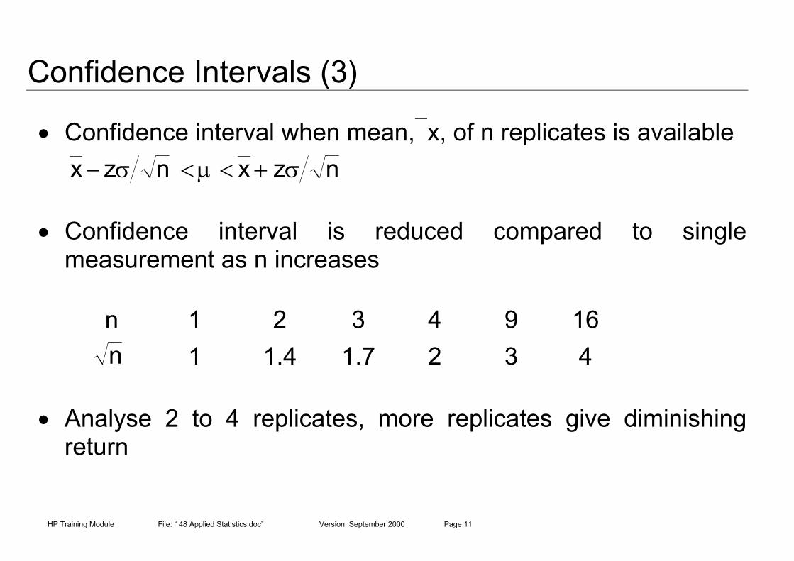
• Confidence interval when mean,x, of n replicates is available

• Confidence interval is reduced compared to singlemeasurement as n increases

n 1 2 3 4 9 16

1 1.4 1.7 2 3 4

• Analyse 2 to 4 replicates, more replicates give diminishingreturn

nzxnzx σ+<µ<σ−

n


Example (2)

• Average mercury conc. from 3 replicates was 1.67 µg/ kg

• Calculate limits for 95% confidence level, σ = 0.1 µg/ kg

1.67 – 1.96 x 0.1/ < µ < 1.67 + 1.96 x 0.1/

1.56 < µ < 1.78

3 3


Example (3)

• How Many replicate analyses will be required to decrease the95% confidence interval to ± 0.07, σ = 0.1

Interval = ± zσ/

± 0.07 = ± 1.96 x 0.1/

n = 7.8

• 8 measurements will give slightly better than 95% chance for µto be with x ± 0.07

n

n


Confidence Interval (4)

• When σ is unknown

• Sample s based on n measurements is available

Degrees of Freedom 1 4 10 αT95 12.7 2.78 2.23 1.96

T99 63.7 4.60 3.17 2.58

• Note T → z as degrees of freedom increases to ∝

nstxnstx +<µ<−


Example (4)

• Groundwater samples were analysed for TOC, n = 5, x = 11.7mg/L s = 3.2 mg/L

• Find the 95% confidence limit for the true mean

- Degrees of freedom = n – 1 = 5 – 1 = 4

- T95 = 2.78 (from table)

11.7 – 2.78 x 3.2 / < µ < 11.7 + 2.78 x 3.2 /

7 < µ < 15.74

5 5


Detection of Outliers

• Extreme values, very high or low, will influence calculatedstatistics

• Rejection

- sound basis

- may be due to an unrecorded event

- errors in transcription, reading of instruments, inconsistentmethodology, etc.

- otherwise apply statistical yardsticks


Q Test

• Qexp =

• Reject if Qexp = Qcrit

Total No. ofobservations

3 5 7 10

Qcrit 90% 0.94 0.64 0.51 0.41

Qcrit 96% 0.98 0.73 0.59 0.48

• Other criteria are also available

testentireofSpreadneighbourandsuspectbetweenDifference


Regression Analysis

• Quantification of relationships between variables

- used for predictions

- calibration of instruments

• Least-square method

- deviations due to random errors

y = a + bx

- linear relationship


Calibration of GC

Pesticide conc., µg/L(xi)

Peak area, cm2

(yi)xi

2 yi2 xiyi

0.352 1.09 0.12390 1.1881 0.38680.803 1.78 0.64481 3.1684 1.429341.08 2.60 1.16640 6.7600 2.808001.38 3.03 1.90140 9.1809 4.181401.75 4.01 3.06250 16.0801 7.01750

∑ 5.365 12.51 6.90201 36.3775 15.81992

Sxx = ∑xi2 – (∑xi)

2/n =1.145365Syy = ∑yi

2 – (∑yi)2/n =5.07748

Sxy = ∑xiyi – ∑xi ∑yi /n =2.39669

b = Sxy / Sxx = 2.09

a = y - bx = 0.26

HP

Figure 2 - Calibration Curve

0

0.5

1

1.5

2

2.5

3

3.5

4

4.5

0 0.2 0.4 0.6 0.8 1 1.2 1.4 1.6 1.8 2

Concentration of pesticide, ug/L

Pea

k ar

ea,

cm2

Calibration Curve

Training Module File: “ 48 Applied Statistics.doc” Version: September 2000 Page 20


5. Evaluation sheets


6. Handout


Applied Statistics

• Confidence intervals

• Number of replicate observations

• Rejection of data

• Regression analysis


• Population mean µ is always unknown

• Sample mean x- Only for large number of replicate x → µ

• Estimation of limits for µ from x(x – a) < µ < (x + a)

• Value of a depend- confidence level (probability of occurrence)- standard deviation- difference between limits is the interval

Confidence Intervals




• When s is good estimate of σ- for single observation, (x - zσ) < µ < (x - zσ)

Confidence level 50 90 95 99 99.7

Z 0.67 1.64 1.96 2.58 3

- as z or interval increases confidence level also increases

Example (1)

• Mercury concentration in fish was determined as 1.8 µg/kg.

• Calculate limits for µ for 95% confidence level if σ = 0.1 µg/k- For 95% confidence level z = 1.96- Limits for mean

1.8 – 1.96 x 0.1 < µ < 1.8 + 1.96 x 0.1

1.6 < µ < 2.0

• What are the limits for 99.7% confidence level?


• Confidence interval when mean,x, of n replicates is available

• Confidence interval is reduced compared to single measurement as n increases

n 1 2 3 4 9 16

1 1.4 1.7 2 3 4

• Analyse 2 to 4 replicates, more replicates give diminishing return

Example (2)

• Average mercury conc. from 3 replicates was 1.67 µg/ kg.

• Calculate limits for 95% confidence level, σ = 0.1 µg/ k

nzxnzx σ+<µ<σ−

n

78.156.1

31.0x96.167.131.0x96.167.1

<µ<+<µ<−


Example (3)

• How Many replicate analyses will be required to decrease the 95% confidenceinterval to ± 0.07, σ = 0.1

Interval = ± zσ/

± 0.07 = ± 1.96 x 0.1/

n = 7.8

• 8 measurements will give slightly better than 95% chance for µ to be with x ±0.07


• When σ is unknown

• Sample s based on n measurements is available

Degrees of Freedom 1 4 10 α

T95 12.7 2.78 2.23 1.96

T99 63.7 4.60 3.17 2.58

• Note T → z as degrees of freedom increases to α

Example (4)

• Groundwater samples were analysed for TOC n = 5, x = 11.7 mg/L s = 3.2mg/L

• Find the 95% confidence limit for the true mean- Degrees of freedom = n – 1 = 5 – 1 = 4- T95 = 2.78

11.7 – 2.78 x 3.2 / < µ < 11.7 + 2.78 x 3.2 /7 < µ < 15.74

n

n

nstxnstx +<µ<−

5 5


Detection of Outliers

• Extreme values, very high or low, will influence calculated statistics

• Rejection- sound basis- may be due to an unrecorded event- errors in transcription, reading of instruments, inconsistent methodology, etc.- otherwise apply statistical yardsticks

Q Test

• Qexp =

• Reject if Qexp = Qcrit

Total No. ofobservations

3 5 7 10

Qcrit 90% 0.94 0.64 0.51 0.41

Qcrit 96% 0.98 0.73 0.59 0.48

• Other criteria are also available

Regression Analysis

• Quantification of relationships between variables- used for predictions- calibration of instruments

• Least-square method- deviations due to random errors

y = a + bx- linear relationship

testentireofSpread

neighbourandsuspectbetweenDifference


Calibration of GC

Pesticide conc.,µg/L(xi)

Peak area,cm2 (yi)

xi2 yi

2 xiyi

0.352 1.09 0.12390 1.1881 0.38680.803 1.78 0.64481 3.1684 1.429341.08 2.60 1.16640 6.7600 2.808001.38 3.03 1.90140 9.1809 4.181401.75 4.01 3.06250 16.0801 7.01750

∑ 5.365 12.51 6.90201 36.3775 15.81992

Sxx = ∑xi2 – (∑xi)

2/n =1.145365Syy = ∑yi

2 – (∑yi)2/n =5.07748

Sxy = ∑xiyi – ∑xi ∑yi /n =2.39669

b = Sxy / Sxx = 2.09

a = y - bx = 0.26

Figure 2 – Calibration Curve

0

0.5

1

1.5

2

2.5

3

3.5

4

4.5

0 0.2 0.4 0.6 0.8 1 1.2 1.4 1.6 1.8 2

Concentration of pesticide,

Pea

k ar

ea, c

m2


Add copy of Main text in chapter 8, for all participants.


7. Additional handoutThese handouts are distributed during delivery and contain test questions, answers toquestions, special worksheets, optional information, and other matters you would not like tobe seen in the regular handouts.

It is a good practice to pre-punch these additional handouts, so the participants can easilyinsert them in the main handout folder.


8. Main text

Contents

1. Confidence Intervals 1

2. Detection of Data Outliers 5

3. Regression Analysis 6


Applied Statistics

For small data sets, there is always the question as to how well the data represent thepopulation and what useful information can be inferred regarding the populationcharacteristics. Statistical calculations are used for this purpose. This module deals with foursuch applications:

1. Definition of a population around the mean of a data set within which the true mean canbe expected to be found with a particular degree of probability.

2. Determination of the number of measurements needed to obtain the true mean within apredetermined interval around the experimental mean with a particular degree ofprobability.

3. Determining if an outlying value in a set of replicate measurements should be retained incalculating the mean for the set.

4. The fitting of a straight line to a set of experimental points.

1. Confidence Intervals

The true mean of population, µ, is always unknown. However, limits can be set about theexperimentally determined mean, x, within which the true mean may be expected to occurwith a given degree of probability. These bounds are called confidence limits and the intervalbetween these limits, the confidence interval.

For a given set of data, if the confidence interval about the mean is large, the probability ofan observation falling within the limits also becomes large. On the other hand, in the casewhen the limits are set close to the mean, the probability that the observed value falls withinthe limits also becomes smaller or, in other words, a larger fraction of observations areexpected to fall out side the limits. Usually confidence intervals are calculated such that 95%of the observations are likely to fall within the limits.

For a given probability of occurrence, the confidence limits depend on the value of thestandard deviation, s, of the observed data and the certainty with which this quantity can betaken to represent the true standard deviation, σ, of the population.

1.1 Confidence limits where σ is known

When the number of repetitive observations is 20 or more, the standard deviation of theobserved set of data, s, can be taken to be a good approximation of the standard deviationof the population, σ.

However, it may not always be possible to perform such a large number of repetitiveanalyses, particularly when costly and time consuming extraction and analytical proceduresare involved. In such cases, data from previous records or different laboratories may bepooled, provided that identical precautions and analytical steps are followed in each case.Further, care should be taken that the medium sampled is also similar, for example, analysisresults of groundwater samples having high TDS should not be pooled with the results ofsurface waters, which usually have low TDS.

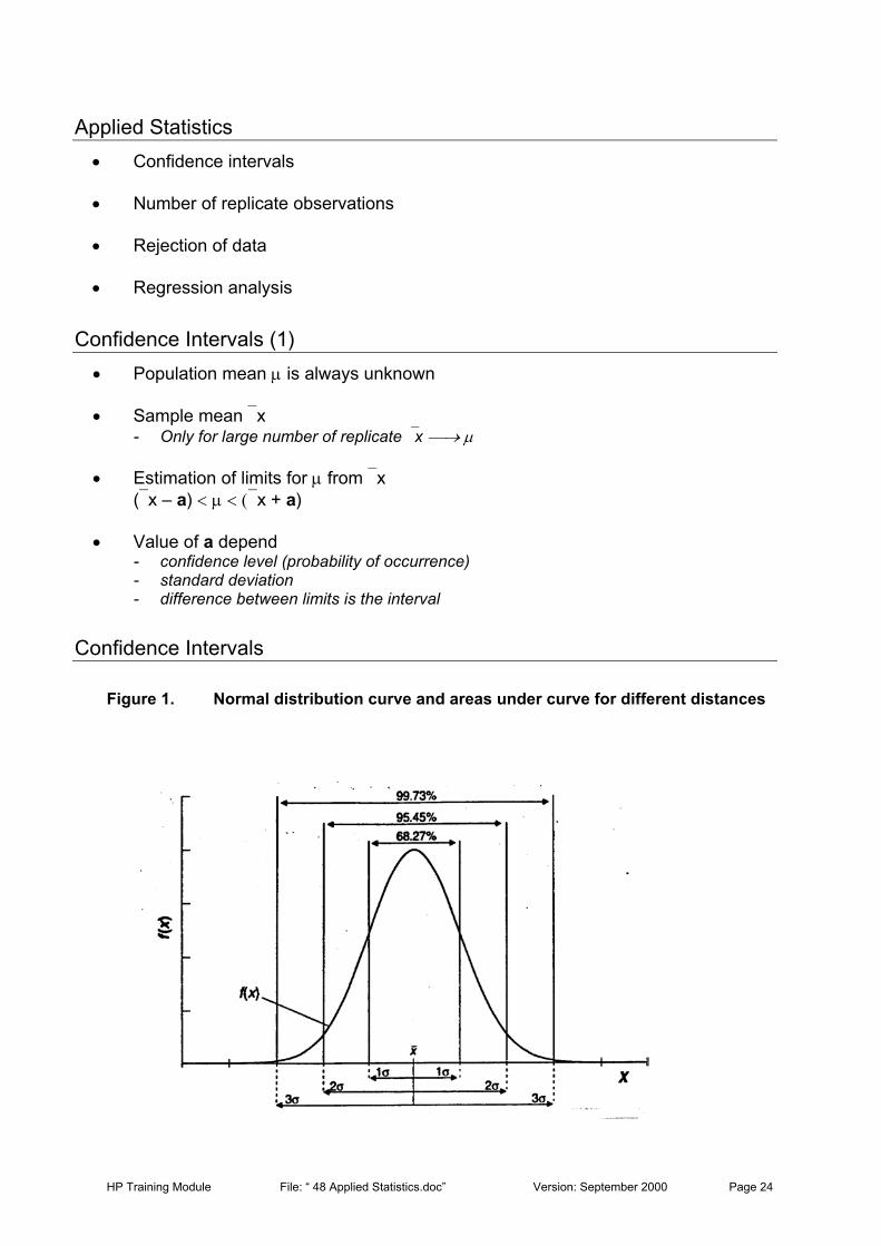
As discussed in the previous module, most of the randomly varying data can beapproximated to a normal distribution curve. For normal distribution, 68% of the observationslie between the limits µ ± σ , 96% between the limits µ ± 2σ, 99.7% between the limits µ ±


3σ, etc., Figure 1. For a single observation, xi, the confidence limits for the population meanare given by:


confidence limit for µ = xi ± zσ (1)

where z assumes different values depending upon the desired confidence level as given inTable 1.

Table 1: Values of z for various confidence levels

Confidence level, % z50 0.6768 1.0080 1.2990 1.6495 1.9696 2.0099 2.58

99.7 3.0099.9 3.29

Example 1:Mercury concentration in the sample of a fish was determined to be 1.80 µg/kg. Calculatethe 50% and 95% confidence limits for this observation. Based on previous analysis records,it is known that the standard deviation of such observations, following similar analysisprocedures, is 0.1 µg/kg and it closely represents the population standard deviation, σ.


From Table 1, it is seen that z = 0.67 and 1.96 for the two confidence limits in question.Upon substitution in Equation 1, we find that

50% confidence limit = 1.80 ± 0.67 x 0.1 = 1.8 ± 0.07 µg/kg95% confidence limit = 1.80 ± 1.96 x 0.1 = 1.8 ± 0.2 µg/kg

Therefore if 100 replicate analyses are made, the results of 50 analysis will lie between thelimits 1.73 and 1.87 and 95 results are expected to be within an enlarged limit of 1.6 and 2.0

Equation 1 applies to the result of a single measurement. In case a number of observations,n, is made and an average of the replicate samples is taken, the confidence intervaldecreases. In such a case the limits are given by:

confidence limit for µ = x ± zσ/ √n (2)

Example 2:Calculate the confidence limits for the problem of Example 1, if three samples of the fishwere analysed yielding an average of 1.67 µg/kg Hg.

Substitution in Equation 2 gives:

50% confidence limit = 1.67 ± 0.67 x 0.1/ √3 = 1.67 ± 0.04 µg/kg95% confidence limit = 1.67 ± 1.96 x 0.1/ √3 = 1.67 ± 0.11 µg/kg

For the same odds the confidence limits are now substantially smaller and the result can besaid to be more accurate and probably more useful.

Note that Equation 2 indicates that the confidence interval can be halved by increasing thenumber of analyses to 4 (√4 = 2) compared to a single observation. Increasing the numberof measurements beyond 4 does not decrease the confidence interval proportionately. Tonarrow the interval by one fourth, 16 measurements would be required (√16 = 4), thus givingdiminishing return. Consequently, 2 to 4 replicate measurements are made in most cases.

Equation 2 can also be used to find the number of replicate measurements required suchthat with a given probability the true mean would be found within a predetermined interval.This is illustrated in Example 3.

Example 3:How many replicate measurements of the specimen in Example 1 would be needed todecrease the 95% confidence interval to ±0.07.

Substituting for confidence interval in Equation 2:

0.07 = 1.96 x 0.1/ √n√n = 1.96 x 0.1/0.07, n = 7.8

Thus, 8 measurements will provide slightly better than 95% chance of he true mean lyingwithin ±0.07 of the experimental mean.


1.2 Confidence limits where σ is unknown

When the number of individual measurements in a set of data are small the reproducibility ofthe calculated value of the standard deviation, s, is decreased. Therefore, for a givenprobability, the confidence interval must be larger under these circumstances.

To account for the potential variability in s, the confidence limits are calculated using thestatistical parameter t:

confidence limit for µ = x ± ts/ √n (3)

In contrast to z in Equation 2, t depends not only on the desired confidence level, but alsoupon the number of degrees of freedom available in the calculation of s. Table 2 providesvalues for t for various degrees of freedom and confidence levels. Note that the values of tbecome equal to those for z (Table 1) as the number of degrees of freedom becomesinfinite.

Table 2: Values of t for various confidence levels and degrees of freedom

Confidence LevelDegrees ofFreedom 90 95 99

1 6.31 12.7 63.72 2.92 4.30 9.923 2.35 3.18 5.844 2.13 2.78 4.605 2.02 2.57 4.036 1.94 2.45 3.718 1.86 2.31 3.36

10 1.81 2.23 3.1712 1.78 2.18 3.1112 1.78 2.16 3.0614 1.76 2.14 2.98∞ 1.64 1.96 2.58

Example 4:A chemist obtained the following data for the concentration of total organic carbon (TOC) ingroundwater samples: 13.55, 6.39, 13.81, 11.20, 13.88 mg/L. Calculate the 95% confidencelimits for the mean of the data.

Thus, from the given data, n = 5, x = 11.77 and s = 3.2. For degrees of freedom = 5 – 1 = 4and 95% confidence limit, t from Table 2 = 2.78. Therefore, from Equation 3:

confidence limit for µ = x ± ts/ √n = 11.77 ± 2.78 x 3.2/ √5 = 11.77 ± 3.97


2. Detection of Data OutliersData outliers are extreme (high or low) values that diverge widely from the main body of thedata set. The presence of one or more outliers may greatly influence any calculated statisticsand yield biased results. However, there is also the possibility that the outlier is a legitimatemember of the data set. Outlier detection tests are to determine whether there is sufficientstatistical evidence to conclude that an observation appears extreme and does not belong tothe data set and should be rejected.

Data outliers may result from faulty instruments, error in transcription, misreading ofinstruments, inconsistent methodology of sampling and analysis and so on. These aspectsshould be investigated and if any of such reasons can be pegged to an outlier, the valuemay be safely deleted from consideration. However, this is to be kept in mind that thesuspect data may rightfully belong to the set and may be the consequence of an unrecordedevent, such as, a short rainfall, intrusion of sea water or a spill.

Table 3: Critical values for rejection quotient

Qcrit (reject if Qexp> Qcrit)Number of observations90% confidence 96% confidence

3 0.94 0.984 0.76 0.855 0.64 0.736 0.56 0.647 0.51 0.598 0.47 0.549 0.44 0.51

10 0.41 0.48

Of the numerous statistical criteria available for detection of outliers, the Q test, which iscommonly used, will be discussed here. To apply the Q test, the difference between thequestionable result and its closest neighbour is divided by the spread of the entire set. Theresulting ratio Qexp is compared with the rejection values, Qcrit given in Table3, that arecritical for a particular degree of confidence. If Qexp is larger, a statistical basis for rejectionexists. The table shows only some selected values. Any standard statistical analysis bookmay be consulted for a complete set.

Example 5:Concentration measurements for fluoride in a well were measured as 2.77, 2.80, 2.90, 2.92,3.45, 3.95, 4.44, 4.61, 5.21, 7.46. Use the Q test to examine whether the highest value is anoutlier.

Qexp = (7.46 – 5.21) / (7.46 – 2.77) = 0.51Since 0.51 is larger than 0.48, the Qcrit value for 96% confidence, there is a basis forexcluding the value.

Other criteria that can be used to evaluate an apparent outlier are:

- Plotting of a scatter diagram indicating inter-parameter relationship between twoconstituents. If there is a correlation between the two constituents, an outlier would lie asignificant distance from the general trend.


- Applying test for normal distribution by calculating the mean and standard deviation of allthe data and determining if the extreme value is outside the mean ±3 times the standarddeviation limit. If so, it is indeed an unusual value. (A cumulative normal probability plotmay also be used for this test.)

- When the data set is not large, calculating and comparing the standard deviation, withand without the suspect observations. A suspect value which has a considerableinfluence on the calculated standard deviation suggests an outlier.

3. Regression AnalysisIn assessing environmental quality , it is often of interest to quantify relationship between twoor more variables. This may allow filling of missing data for one constituent and also mayhelp in predicting future levels of a constituent.

Regression analysis is focused on determining the degree to which one or more variable(s)is dependant on an other variable, the independent variable. Thus regression is a means ofcalibrating coefficients of a predictive equation. In correlation analysis neither of thevariables is identified as more important than the other. Correlation is not causation. Itprovides a measure of the goodness of fit.

In the calibration step, in most analytical procedures where a ‘best’ straight line is fitted tothe observed response of the detector system when known amounts of analyte (standards)are analysed. This section discusses the regression analysis procedure employed for thispurpose.

Least-squares method is the most straightforward regression procedure. Application of themethod requires two assumptions; a linear relationship exists between the amount of analyte(x) and the magnitude of the measured response (y) and that any deviation of individualpoints from the straight line is entirely the consequence of indeterminate error, that is, nosignificant error exists in the composition of the standards.

The line generated is of the form:

y = a + bx (4)

where a is the value of y when x is zero (the intercept) and b is the slope. The methodminimises the squares of the vertical displacements of data points from the best fit line.

For convenience, the following three quantities are defined:

Sxx = ∑ (xi – x)2 = ∑xi2 – (∑xi)

2/nSyy = ∑ (yi – y)2 = ∑yi

2 – (∑yi)2/n

Sxy = ∑ (xi – x) (yi – y) = ∑xiyi – ∑xi ∑yi /n

Calculating these quantities permits the determination of the following:

1. The slope of the line b:

b = Sxy/Sxx (5)

2. The intercept a:

a = y – bx (6)

3. The standard deviation about the regression line, sr:

sr = √{(Syy – b2Sxx)/(n-2)} (7)

4. The standard deviation of the slope sb:

sb = √(sr2/Sxx) (8)

5. The standard deviation of the results based on the calibration curve sc:

sc = (sr/b) x √{(1/m) + (1/n) + (yc – y)2/b2Sxx} (9)

where yc is the mean of m replicate measurements made using the calibration curve.

Example 6:The following table gives calibration data for chromatographic analysis of a pesticide andcomputations for fitting a straight line according to the least-square method.

Pesticide conc., µg/L(xi)

Peak area, cm2 (yi) xi2 yi

2 xiyi

0.352 1.09 0.12390 1.1881 0.38680.803 1.78 0.64481 3.1684 1.429341.08 2.60 1.16640 6.7600 2.808001.38 3.03 1.90140 9.1809 4.181401.75 4.01 3.06250 16.0801 7.01750

∑ 5.365 12.51 6.90201 36.3775 15.81992

Therefore

Sxx = ∑xi2 – (∑xi)

2/n =1.145365Syy = ∑yi

2 – (∑yi)2/n =5.07748

Sxy = ∑xiyi – ∑xi ∑yi /n =2.39669

and from Equations 5 & 6

b = 2.0925 = 2.09 and a = 0.2567 = 0.26

Thus the equation for the least-square line is

y = 0.26 + 2.09x

Note that rounding should not be performed until the end in order to avoid rounding errors.

The data points and the equation is plotted in Figure2.



Figure 2: Calibration Curve

Example 7:Using the relationship derived in Example 6 calculate

1. concentration of pesticide in sample if the peak area of 2.65 was obtained.2. the standard deviation of the result based on the single measurement of 2.65.3. the standard deviation of the measurement if 2.65 represents the average of 4

replicates.

1. Substituting in the equation derived in the previous example

2.65 = 0.26 + 2.09xx = 1.14 µg/L

2. Substituting in Equation 9 for m = 1

sc = (0.144/2.09) x √{(1/1) + (1/5) + (2.65 – 12.51/5)2/2.092 x1.145} = ±0.08

3. Substituting in Equation 9 for m = 4

sc = (0.144/2.09) x √{(1/4) + (1/5) + (2.65 – 12.51/5)2/2.092 x1.145} = ±0.05

0

0.5

1

1.5

2

2.5

3

3.5

4

4.5

0 0.2 0.4 0.6 0.8 1 1.2 1.4 1.6 1.8 2

Concentration of pesticide, ug/L

Pea

k ar

ea, c

m2

download-manuals-surface water-software-48appliedstatistics

Technology

module contextthis module

minhp training module

module profiletitle

org jpshp training module

training course

depth of training

prior training

training needs