douglas m. bates 2005{2012; - eth z
TRANSCRIPT

lme4: Mixed-effects modeling with R
Douglas M. Bates
2005–2012; small changes 2018 – LATEX’ed March 15, 2022


To Phyl and Dave, with thanks for your kind hospitality. You see, I really was“working” when I was sitting on your deck staring at the lake.

ii

Preface
R is a freely available implementation of John Chambers’ award-winning S language forcomputing with data. It is “Open Source” software for which the user can, if she wishes,obtain the original source code and determine exactly how the computations are beingperformed. Most users of R use the precompiled versions that are available for recentversions of the Microsoft Windows operating system, for Mac OS X, and for several versionsof the Linux operating system. Directions for obtaining and installing R are on https:
//www.R-project.org or https://cran.R-project.org.Because it is freely available, R is accessible to anyone who cares to learn to use it, and
thousands have done so. Recently many prominent social scientists, including John Foxof McMaster University and Gary King of Harvard University, have become enthusiasticR users and developers.
Another recent development in the analysis of social sciences data is the recognitionand modeling of multiple levels of variation in longitudinal and organizational data. Theclass of techniques for modeling such levels of variation has become known as multilevelmodeling or hierarchical linear modeling.
In this book I describe the use of R for examining, managing, visualizing, and modelingmultilevel data.
Madison, WI, USA, Douglas BatesOctober, 2005
iii

iv Preface

Contents
Preface iii
Acronyms xi
1 A Simple, Linear, Mixed-effects Model 1
1.1 Mixed-effects Models . . . . . . . . . . . . . . . . . . . . . . . . . . . . . . . 1
1.2 The Dyestuff and Dyestuff2 Data . . . . . . . . . . . . . . . . . . . . . . 2
1.2.1 The Dyestuff Data . . . . . . . . . . . . . . . . . . . . . . . . . . . 2
1.2.2 The Dyestuff2 Data . . . . . . . . . . . . . . . . . . . . . . . . . . . 5
1.3 Fitting Linear Mixed Models . . . . . . . . . . . . . . . . . . . . . . . . . . 6
1.3.1 A Model For the Dyestuff Data . . . . . . . . . . . . . . . . . . . . 6
1.3.2 A Model For the Dyestuff2 Data . . . . . . . . . . . . . . . . . . . 8
1.3.3 Further Assessment of the Fitted Models . . . . . . . . . . . . . . . 10
1.4 The Linear Mixed-effects Probability Model . . . . . . . . . . . . . . . . . . 11
1.4.1 Definitions and Results . . . . . . . . . . . . . . . . . . . . . . . . . 11
1.4.2 Matrices and Vectors in the Fitted Model Object . . . . . . . . . . . 12
1.5 Assessing the Variability of the Parameter Estimates . . . . . . . . . . . . . 15
1.5.1 Confidence Intervals on the Parameters . . . . . . . . . . . . . . . . 15
1.5.2 Interpreting the Profile Zeta Plot . . . . . . . . . . . . . . . . . . . . 17
1.5.3 Deriving densities from the profile . . . . . . . . . . . . . . . . . . . 18
1.6 Assessing the Random Effects . . . . . . . . . . . . . . . . . . . . . . . . . . 19
1.7 Chapter Summary . . . . . . . . . . . . . . . . . . . . . . . . . . . . . . . . 22
Notation . . . . . . . . . . . . . . . . . . . . . . . . . . . . . . . . . . . . . . . . . 22
Exercises . . . . . . . . . . . . . . . . . . . . . . . . . . . . . . . . . . . . . . . . 23
2 Models With Multiple Random-effects Terms 25
2.1 A Model With Crossed Random Effects . . . . . . . . . . . . . . . . . . . . 25
2.1.1 The Penicillin Data . . . . . . . . . . . . . . . . . . . . . . . . . . 25
2.1.2 A Model For the Penicillin Data . . . . . . . . . . . . . . . . . . . 28
2.2 A Model With Nested Random Effects . . . . . . . . . . . . . . . . . . . . . 34
2.2.1 The Pastes Data . . . . . . . . . . . . . . . . . . . . . . . . . . . . . 34
2.2.2 Fitting a Model With Nested Random Effects . . . . . . . . . . . . . 37
2.2.3 Parameter Estimates for Model fm04 . . . . . . . . . . . . . . . . . . 39
2.2.4 Testing H0 : σ2 = 0 Versus Ha : σ2 > 0 . . . . . . . . . . . . . . . . . 40
2.2.5 Assessing the Reduced Model, fm04a . . . . . . . . . . . . . . . . . . 41
2.3 A Model With Partially Crossed Random Effects . . . . . . . . . . . . . . . 43
2.3.1 The InstEval Data . . . . . . . . . . . . . . . . . . . . . . . . . . . 43
2.3.2 Structure of L for model fm05 . . . . . . . . . . . . . . . . . . . . . . 46
2.4 Chapter Summary . . . . . . . . . . . . . . . . . . . . . . . . . . . . . . . . 47
Exercises . . . . . . . . . . . . . . . . . . . . . . . . . . . . . . . . . . . . . . . . 48
v

vi CONTENTS
3 Models for Longitudinal Data 51
3.1 The sleepstudy Data . . . . . . . . . . . . . . . . . . . . . . . . . . . . . . 51
3.1.1 Characteristics of the sleepstudy Data Plot . . . . . . . . . . . . . 53
3.2 Mixed-effects Models For the sleepstudy Data . . . . . . . . . . . . . . . . 54
3.2.1 A Model With Correlated Random Effects . . . . . . . . . . . . . . 54
3.2.2 A Model With Uncorrelated Random Effects . . . . . . . . . . . . . 56
3.2.3 Generating Z and Λ From Random-effects Terms . . . . . . . . . . . 59
3.2.4 Comparing Models fm07 and fm06 . . . . . . . . . . . . . . . . . . . 60
3.3 Assessing the Precision of the Parameter Estimates . . . . . . . . . . . . . . 60
3.4 Examining the Random Effects and Predictions . . . . . . . . . . . . . . . . 63
3.5 Chapter Summary . . . . . . . . . . . . . . . . . . . . . . . . . . . . . . . . 68
Problems . . . . . . . . . . . . . . . . . . . . . . . . . . . . . . . . . . . . . . . . 68
4 Building Linear Mixed Models 71
4.1 Incorporating categorical covariates with fixed levels . . . . . . . . . . . . . 71
4.1.1 The Machines Data . . . . . . . . . . . . . . . . . . . . . . . . . . . 71
4.1.2 Comparing models with and without interactions . . . . . . . . . . . 72
4.1.3 Coefficients for factors in the fixed effects . . . . . . . . . . . . . . . 74
4.2 Models for the ergoStool data . . . . . . . . . . . . . . . . . . . . . . . . . 76
4.2.1 Random-effects for both Subject and Type . . . . . . . . . . . . . . 77
4.2.2 Fixed Effects for Type, Random for Subject . . . . . . . . . . . . . 80
4.2.3 Fixed Effects for Type and Subject . . . . . . . . . . . . . . . . . . 85
4.2.4 Fixed Effects Versus Random Effects for Subject . . . . . . . . . . . 86
4.3 Covariates Affecting Mathematics Score Gain . . . . . . . . . . . . . . . . . 87
4.4 Rat Brain example . . . . . . . . . . . . . . . . . . . . . . . . . . . . . . . . 90
5 Computational Methods for Mixed Models 93
5.1 Definitions and Basic Results . . . . . . . . . . . . . . . . . . . . . . . . . . 93
5.2 The Conditional Distribution (U|Y = y) . . . . . . . . . . . . . . . . . . . . 95
5.3 Integrating h(u) in the Linear Mixed Model . . . . . . . . . . . . . . . . . . 95
5.4 Determining the PLS Solutions, u and βθ . . . . . . . . . . . . . . . . . . . 97
5.4.1 The Fill-reducing Permutation, P . . . . . . . . . . . . . . . . . . . 97
5.4.2 The Value of the Deviance and Profiled Deviance . . . . . . . . . . . 98
5.4.3 Determining r2θ and βθ . . . . . . . . . . . . . . . . . . . . . . . . . . 100
5.5 The REML Criterion . . . . . . . . . . . . . . . . . . . . . . . . . . . . . . . 100
5.6 Step-by-step Evaluation of the Profiled Deviance . . . . . . . . . . . . . . . 102
5.7 Generalizing to Other Forms of Mixed Models . . . . . . . . . . . . . . . . . 106
5.7.1 Descriptions of the Model Forms . . . . . . . . . . . . . . . . . . . . 106
5.7.2 Determining the Conditional Mode, u . . . . . . . . . . . . . . . . . 107
5.8 Chapter Summary . . . . . . . . . . . . . . . . . . . . . . . . . . . . . . . . 108
Exercises . . . . . . . . . . . . . . . . . . . . . . . . . . . . . . . . . . . . . . . . 108
6 Generalized Linear Mixed Models for Binary Responses 111
6.1 Artificial contraception use in regions of Bangladesh . . . . . . . . . . . . . 111
6.1.1 Plotting the binary response . . . . . . . . . . . . . . . . . . . . . . 112
6.1.2 Initial GLMM fit to the contraception data . . . . . . . . . . . . . . 113
6.2 Link functions and interpreting coefficients . . . . . . . . . . . . . . . . . . 117
6.2.1 The logit link function for binary responses . . . . . . . . . . . . . . 118
6.2.2 Canonical link functions . . . . . . . . . . . . . . . . . . . . . . . . . 118
6.2.3 Interpreting coefficient estimates . . . . . . . . . . . . . . . . . . . . 119

CONTENTS vii
A Examining likelihood contour projections 123A.0.1 Profile Pairs Plots . . . . . . . . . . . . . . . . . . . . . . . . . . . . 123
Exercises . . . . . . . . . . . . . . . . . . . . . . . . . . . . . . . . . . . . . . . . 125

viii CONTENTS

List of Figures
1.1 Yield of dyestuff from 6 batches of an intermediate . . . . . . . . . . . . . . 4
1.2 Simulated data similar in structure to the Dyestuff data . . . . . . . . . . . 5
1.3 Image of the Λ for model fm01ML . . . . . . . . . . . . . . . . . . . . . . . . 14
1.4 Image of the random-effects model matrix, ZT, for fm01 . . . . . . . . . . . 14
1.5 Profile zeta plots of the parameters in model fm01ML . . . . . . . . . . . . . 16
1.6 Absolute value profile zeta plots of the parameters in model fm01ML . . . . . 16
1.7 Profile zeta plots comparing log(σ), σ and σ2 in model fm01ML . . . . . . . . 17
1.8 Profile zeta plots comparing log(σ1), σ1 and σ21 in model fm01ML . . . . . . . 18
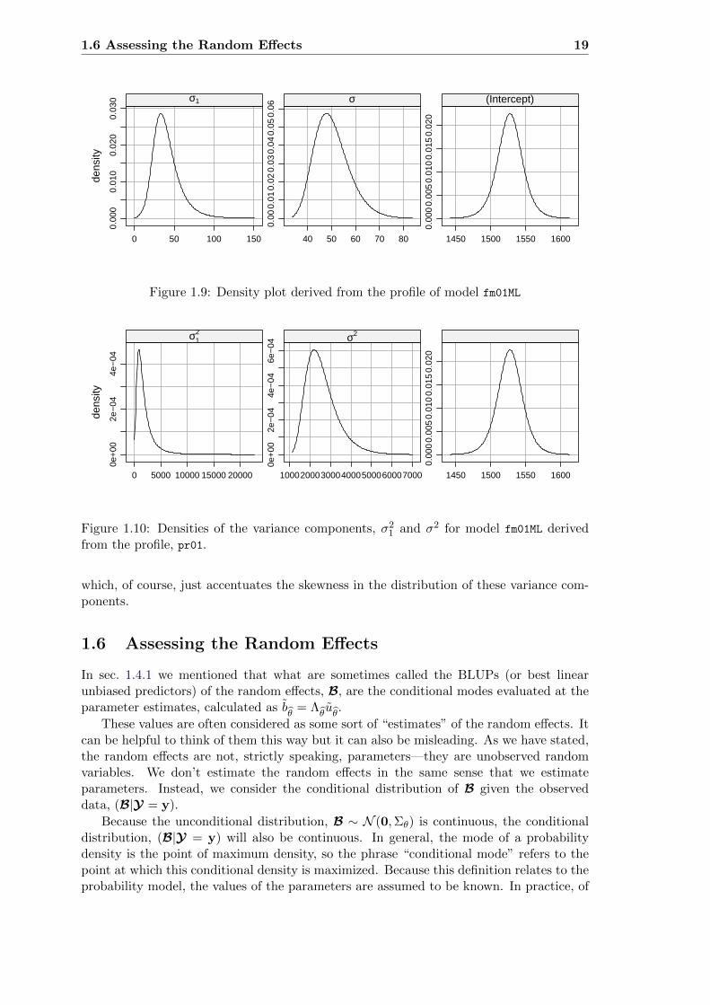
1.9 Density plot derived from the profile of model fm01ML . . . . . . . . . . . . . 19
1.10 Variance component density plot for model fm01ML . . . . . . . . . . . . . . 19
1.11 95% prediction intervals on the random effects in fm01ML, shown as a dotplot 21
1.12 95% prediction intervals on the random effects in fm01ML versus quantilesof the standard normal distribution . . . . . . . . . . . . . . . . . . . . . . . 21
1.13 Travel time for an ultrasonic wave test on 6 rails . . . . . . . . . . . . . . . 24
2.1 Diameter of growth inhibition zone for 6 samples of penicillin . . . . . . . . 27
2.2 Random effects prediction intervals for model fm03 . . . . . . . . . . . . . . 29
2.3 Image of the random-effects model matrix for fm03 . . . . . . . . . . . . . . 29
2.4 Images of Λ, ZTZ and L for model fm03 . . . . . . . . . . . . . . . . . . . . 30
2.5 Profile zeta plot of the parameters in model fm03 . . . . . . . . . . . . . . . 30
2.6 Profile pairs plot of the parameters in model fm03. . . . . . . . . . . . . . . 32
2.7 Profile pairs plot for model fm03 (log scale) . . . . . . . . . . . . . . . . . . 33
2.8 Cross-tabulation image of the batch and sample factors . . . . . . . . . . . . 35
2.9 Strength of paste preparations by batch and sample . . . . . . . . . . . . . 36
2.10 Images of Λ, ZTZ and L for model fm04 . . . . . . . . . . . . . . . . . . . . 38
2.11 Random effects prediction intervals for model fm04 . . . . . . . . . . . . . . 39
2.12 Profile zeta plots for the parameters in model fm04 . . . . . . . . . . . . . . 40
2.13 Profile zeta plots for the parameters in model fm04a . . . . . . . . . . . . . 42
2.14 Profile pairs plot of the parameters in model fm04a. . . . . . . . . . . . . . . 43
2.15 Random effects prediction intervals for model fm05 . . . . . . . . . . . . . . 45
2.16 Image of the sparse Cholesky factor, L, from model fm05 . . . . . . . . . . . 46
3.1 Lattice plot of the sleepstudy data . . . . . . . . . . . . . . . . . . . . . . . 52
3.2 Images of Λ, Σ and L for model fm06 . . . . . . . . . . . . . . . . . . . . . . 55
3.3 Images of Λ, Σ and L for model fm07 . . . . . . . . . . . . . . . . . . . . . . 58
3.4 Images of ZT for models fm06 and fm07 . . . . . . . . . . . . . . . . . . . . . 58
3.5 Profile zeta plots for the parameters in model fm07 . . . . . . . . . . . . . . 61
3.6 Profile pairs plot for the parameters in model fm07 . . . . . . . . . . . . . . 62
3.7 Plot of the conditional modes of the random effects for model fm07 (leftpanel) and the corresponding subject-specific coefficients (right panel) . . . 64
ix

x LIST OF FIGURES
3.8 Comparison of within-subject estimates and conditional modes for fm07 . . 663.9 Comparison of predictions from separate fits and fm07 . . . . . . . . . . . . 673.10 Prediction intervals on the random effects for model fm07 . . . . . . . . . . 693.11 Distance versus height for female Orthodont subjects . . . . . . . . . . . . . 69
4.1 Quality score by operator and machine . . . . . . . . . . . . . . . . . . . . . 724.2 Random effects prediction intervals for model fm10 . . . . . . . . . . . . . . 744.3 Effort to arise by subject and stool type . . . . . . . . . . . . . . . . . . . . 774.4 Profile zeta plot for the parameters in model fm16 . . . . . . . . . . . . . . . 784.5 Profile pairs plot for the parameters in model fm16 . . . . . . . . . . . . . . 794.6 Prediction intervals on the random effects for stool type . . . . . . . . . . . 804.7 Profile zeta plot for the parameters in model fm16 . . . . . . . . . . . . . . . 834.8 Comparative dotplots of gain in the mathematics scores in classrooms within
schools . . . . . . . . . . . . . . . . . . . . . . . . . . . . . . . . . . . . . . . 894.9 Profile plot of the parameters in model fm4 . . . . . . . . . . . . . . . . . . 904.10 Activation of brain regions in rats . . . . . . . . . . . . . . . . . . . . . . . 91
6.1 Contraception use versus centered age . . . . . . . . . . . . . . . . . . . . . 1126.2 Contraception use versus centered age (children/no children) . . . . . . . . 1156.3 Inverse of the logit link function . . . . . . . . . . . . . . . . . . . . . . . . 1196.4 95% prediction intervals on the random effects in fm13 versus quantiles of
the standard normal distribution. . . . . . . . . . . . . . . . . . . . . . . . . 120
A.1 Profile pairs plot for the parameters in model fm01 . . . . . . . . . . . . . . 124

Acronyms
AIC Akaike’s Information Criterion
AMD Approximate Minimal Degree
BIC Bayesian Information Criterion (also called “Schwatz’s Bayesian Information Crite-rion”)
BLUP Best Linear Unbiased Predictor
GLMM Generalized Linear Mixed Model
LMM Linear Mixed Model
LRT Likelihood Ratio Test
ML Maximum Likelihood
MLE Maximum Likelihood Estimate or Maximum Likelihood Estimator
NLMM NonLinear Mixed Model
REML The REstricted (or “REsidual”) Maximum Likelihood estimation criterion
PRSS Penalized, Residual Sum-of-Squares
PWRSS Penalized, Weighted, Residual Sum-of-Squares
xi

xii Acronyms

Chapter 1
A Simple, Linear, Mixed-effectsModel
In this book we describe the theory behind a type of statistical model called mixed-effectsmodels and the practice of fitting and analyzing such models using the lme4 package forR. These models are used in many different disciplines. Because the descriptions of themodels can vary markedly between disciplines, we begin by describing what mixed-effectsmodels are and by exploring a very simple example of one type of mixed model, the linearmixed model.
This simple example allows us to illustrate the use of the lmer function in the lme4
package for fitting such models and for analyzing the fitted model. We also describe meth-ods of assessing the precision of the parameter estimates and of visualizing the conditionaldistribution of the random effects, given the observed data.
1.1 Mixed-effects Models
Mixed-effects models, like many other types of statistical models, describe a relationshipbetween a response variable and some of the covariates that have been measured or ob-served along with the response. In mixed-effects models at least one of the covariates isa categorical covariate representing experimental or observational “units” in the data set.In the example from the chemical industry that is given in this chapter, the observationalunit is the batch of an intermediate product used in production of a dye. In medical andsocial sciences the observational units are often the human or animal subjects in the study.In agriculture the experimental units may be the plots of land or the specific plants beingstudied.
In all of these cases the categorical covariate or covariates are observed at a set ofdiscrete levels. We may use numbers, such as subject identifiers, to designate the particularlevels that we observed but these numbers are simply labels. The important characteristicof a categorical covariate is that, at each observed value of the response, the covariatetakes on the value of one of a set of distinct levels.
Parameters associated with the particular levels of a covariate are sometimes called the“effects” of the levels. If the set of possible levels of the covariate is fixed and reproduciblewe model the covariate using fixed-effects parameters. If the levels that we observedrepresent a random sample from the set of all possible levels we incorporate random effectsin the model.
There are two things to notice about this distinction between fixed-effects parametersand random effects. First, the names are misleading because the distinction between
1

2 A Simple, Linear, Mixed-effects Model
fixed and random is more a property of the levels of the categorical covariate than aproperty of the effects associated with them. Secondly, we distinguish between “fixed-effects parameters”, which are indeed parameters in the statistical model, and “randomeffects”, which, strictly speaking, are not parameters. As we will see shortly, randomeffects are unobserved random variables.
To make the distinction more concrete, suppose that we wish to model the annualreading test scores for students in a school district and that the covariates recorded withthe score include a student identifier and the student’s gender. Both of these are categoricalcovariates. The levels of the gender covariate, male and female, are fixed. If we considerdata from another school district or we incorporate scores from earlier tests, we will notchange those levels. On the other hand, the students whose scores we observed wouldgenerally be regarded as a sample from the set of all possible students whom we couldhave observed. Adding more data, either from more school districts or from results onprevious or subsequent tests, will increase the number of distinct levels of the studentidentifier.
Mixed-effects models or, more simply, mixed models are statistical models that incor-porate both fixed-effects parameters and random effects. Because of the way that we willdefine random effects, a model with random effects always includes at least one fixed-effectsparameter. Thus, any model with random effects is a mixed model.
We characterize the statistical model in terms of two random variables: a q-dimensionalvector of random effects represented by the random variable B and an n-dimensional re-sponse vector represented by the random variable Y . (We use upper-case “script” char-acters to denote random variables. The corresponding lower-case upright letter denotesa particular value of the random variable.) We observe the value, y, of Y . We do notobserve the value, b, of B.
When formulating the model we describe the unconditional distribution of B and theconditional distribution, (Y |B = b). The descriptions of the distributions involve theform of the distribution and the values of certain parameters. We use the observed valuesof the response and the covariates to estimate these parameters and to make inferencesabout them.
That’s the big picture. Now let’s make this more concrete by describing a particu-lar, versatile class of mixed models called linear mixed models and by studying a simpleexample of such a model. First we describe the data in the example.
1.2 The Dyestuff and Dyestuff2 Data
Models with random effects have been in use for a long time. The first edition of theclassic book, Statistical Methods in Research and Production, edited by O.L. Davies, waspublished in 1947 and contained examples of the use of random effects to characterizebatch-to-batch variability in chemical processes. The data from one of these examples areavailable as the Dyestuff data in the lme4 package. In this section we describe and plotthese data and introduce a second example, the Dyestuff2 data, described in Box & Tiao(1973).
1.2.1 The Dyestuff Data
The Dyestuff data are described in Davies & Goldsmith (1972, Table 6.3, p. 131), thefourth edition of the book mentioned above, as coming from
an investigation to find out how much the variation from batch to batch in thequality of an intermediate product (H-acid) contributes to the variation in the

1.2 The Dyestuff and Dyestuff2 Data 3
yield of the dyestuff (Naphthalene Black 12B) made from it. In the experi-ment six samples of the intermediate, representing different batches of worksmanufacture, were obtained, and five preparations of the dyestuff were madein the laboratory from each sample. The equivalent yield of each preparationas grams of standard colour was determined by dye-trial.
To access these data within R we must first attach the lme4 package to our sessionusing
> library(lme4)
Note that the ">" symbol in the line shown is the prompt in R and not part of whatthe user types. The lme4 package must be attached before any of the data sets or functionsin the package can be used. If typing this line results in an error report stating that thereis no package by this name then you must first install the package.
In what follows, we will assume that the lme4 package has been installed and that ithas been attached to the R session before any of the code shown has been run.
The str function in R provides a concise description of the structure of the data
> str(Dyestuff)
'data.frame': 30 obs. of 2 variables:
$ Batch: Factor w/ 6 levels "A","B","C","D",..: 1 1 1 1 1 2 2 2 2 2 ...
$ Yield: num 1545 1440 1440 1520 1580 ...
from which we see that it consists of 30 observations of the Yield, the response variable,and of the covariate, Batch, which is a categorical variable stored as a factor object. Ifthe labels for the factor levels are arbitrary, as they are here, we will use letters instead ofnumbers for the labels. That is, we label the batches as "A" through "F" rather than "1"
through "6". When the labels are letters it is clear that the variable is categorical. Whenthe labels are numbers a categorical covariate can be mistaken for a numeric covariate,with unintended consequences.
It is a good practice to apply str to any data frame the first time you work with itand to check carefully that any categorical variables are indeed represented as factors.
The data in a data frame are viewed as a table with columns corresponding to variablesand rows to observations. The functions head and tail print the first or last few rows (thedefault value of “few” happens to be 6 but we can specify another value if we so choose)
> head(Dyestuff)
Batch Yield
1 A 1545
2 A 1440
3 A 1440
4 A 1520
5 A 1580
6 B 1540
or we could ask for a summary of the data
> summary(Dyestuff)
Batch Yield
A:5 Min. :1440

4 A Simple, Linear, Mixed-effects Model
Yield of dyestuff (grams of standard color)
Bat
ch
F
D
A
B
C
E
1450 1500 1550 1600
Figure 1.1: Yield of dyestuff (Napthalene Black 12B) for 5 preparations from each of 6batches of an intermediate product (H-acid). The line joins the mean yields from thebatches, which have been ordered by increasing mean yield. The vertical positions are“jittered” slightly to avoid over-plotting. Notice that the lowest yield for batch A wasobserved for two distinct preparations from that batch
B:5 1st Qu.:1469
C:5 Median :1530
D:5 Mean :1528
E:5 3rd Qu.:1575
F:5 Max. :1635
Although the summary does show us an important property of the data, namely thatthere are exactly 5 observations on each batch — a property that we will describe by sayingthat the data are balanced with respect to Batch — we usually learn much more about thestructure of such data from plots like Fig. 1.1 than we do from numerical summaries.
In Fig. 1.1 we can see that there is considerable variability in yield, even for prepa-rations from the same batch, but there is also noticeable batch-to-batch variability. Forexample, four of the five preparations from batch F provided lower yields than did any ofthe preparations from batches C and E.
This plot, and essentially all the other plots in this book, were created using DeepayanSarkar’s lattice package for R. In Sarkar (2008) he describes how one would create sucha plot. Because this book was created using Sweave (Leisch, 2002), the exact code used tocreate the plot, as well as the code for all the other figures and calculations in the book,is available on the web site for the book. In sec. 3.1.1 we review some of the principlesof lattice graphics, such as reordering the levels of the Batch factor by increasing meanresponse, that enhance the informativeness of the plot. At this point we will concentrateon the information conveyed by the plot and not on how the plot is created.
In sec. 1.3.1 we will use mixed models to quantify the variability in yield betweenbatches. For the time being let us just note that the particular batches used in thisexperiment are a selection or sample from the set of all batches that we wish to consider.Furthermore, the extent to which one particular batch tends to increase or decrease themean yield of the process — in other words, the “effect” of that particular batch on theyield — is not as interesting to us as is the extent of the variability between batches.For the purposes of designing, monitoring and controlling a process we want to predictthe yield from future batches, taking into account the batch-to-batch variability and the

1.2 The Dyestuff and Dyestuff2 Data 5
Simulated response (dimensionless)
Bat
ch
F
B
D
E
A
C
0 5 10
Figure 1.2: Simulated data presented in Box & Tiao (1973) with a structure similar to thatof the Dyestuff data. These data represent a case where the batch-to-batch variability issmall relative to the within-batch variability.
within-batch variability. Being able to estimate the extent to which a particular batch inthe past increased or decreased the yield is not usually an important goal for us. We willmodel the effects of the batches as random effects rather than as fixed-effects parameters.
1.2.2 The Dyestuff2 Data
The Dyestuff2 data are simulated data presented in Box & Tiao (1973, Table 5.1.4, p.247) where the authors state
These data had to be constructed for although examples of this sort undoubt-edly occur in practice they seem to be rarely published.
The structure and summary
> str(Dyestuff2)
'data.frame': 30 obs. of 2 variables:
$ Batch: Factor w/ 6 levels "A","B","C","D",..: 1 1 1 1 1 2 2 2 2 2 ...
$ Yield: num 7.3 3.85 2.43 9.57 7.99 ...
> summary(Dyestuff2)
Batch Yield
A:5 Min. :-0.892
B:5 1st Qu.: 2.765
C:5 Median : 5.365
D:5 Mean : 5.666
E:5 3rd Qu.: 8.151
F:5 Max. :13.434
are intentionally similar to those of the Dyestuff data. As can be seen in Fig. 1.2the batch-to-batch variability in these data is small compared to the within-batch vari-ability. In some approaches to mixed models it can be difficult to fit models to such data.Paradoxically, small “variance components” can be more difficult to estimate than largevariance components.

6 A Simple, Linear, Mixed-effects Model
The methods we will present are not compromised when estimating small variancecomponents.
1.3 Fitting Linear Mixed Models
Before we formally define a linear mixed model, let’s go ahead and fit models to thesedata sets using lmer. Like most model-fitting functions in R, lmer takes, as its firsttwo arguments, a formula specifying the model and the data with which to evaluate theformula. This second argument, data, is optional but recommended. It is usually thename of a data frame, such as those we examined in the last section. Throughout thisbook all model specifications will be given in this formula/data format.
We will explain the structure of the formula after we have considered an example.
1.3.1 A Model For the Dyestuff Data
We fit a model to the Dyestuff data allowing for an overall level of the Yield and for anadditive random effect for each level of Batch
> fm01 <- lmer(Yield ~ 1 + (1|Batch), Dyestuff)
> summary(fm01)
Linear mixed model fit by REML ['lmerMod']
Formula: Yield ~ 1 + (1 | Batch)
Data: Dyestuff
REML criterion at convergence: 319.7
Scaled residuals:
Min 1Q Median 3Q Max
-1.4117 -0.7634 0.1418 0.7792 1.8296
Random effects:
Groups Name Variance Std.Dev.
Batch (Intercept) 1764 42.00
Residual 2451 49.51
Number of obs: 30, groups: Batch, 6
Fixed effects:
Estimate Std. Error t value
(Intercept) 1527.50 19.38 78.8
In the first line we call the lmer function to fit a model with formula
Yield ~ 1 + (1 | Batch)
applied to the Dyestuff data and assign the result to the name fm01. (The name isarbitrary. I happen to use names that start with fm, indicating “fitted model”.)
As is customary in R, there is no output shown after this assignment. We have simplysaved the fitted model as an object named fm01. In the second line we display someinformation about the fitted model by applying summary to fm01. In later examples we willcondense these two steps into one but here it helps to emphasize that we save the resultof fitting a model then apply various extractor functions to the fitted model to get a briefsummary of the model fit or to obtain the values of some of the estimated quantities.

1.3 Fitting Linear Mixed Models 7
Details of the Printed Display
The printed display of a model fit with lmer has four major sections: a description of themodel that was fit, some statistics characterizing the model fit, a summary of properties ofthe random effects and a summary of the fixed-effects parameter estimates. We considereach of these sections in turn.
The description section states that this is a linear mixed model in which the parametershave been estimated as those that minimize the REML criterion (described in sec. 5.5).The formula and data arguments are displayed for later reference. If other, optionalarguments affecting the fit, such as a subset specification, were used, they too will bedisplayed here.
For models fit by the REML criterion the only statistic describing the model fit isthe value of the REML criterion itself. An alternative set of parameter estimates, themaximum likelihood estimates (MLEs), are obtained by specifying the optional argumentREML=FALSE.
> summary(fm01ML <- lmer(Yield ~ 1 + (1|Batch), Dyestuff,
+ REML=FALSE))
Linear mixed model fit by maximum likelihood ['lmerMod']
Formula: Yield ~ 1 + (1 | Batch)
Data: Dyestuff
AIC BIC logLik deviance df.resid
333.3 337.5 -163.7 327.3 27
Scaled residuals:
Min 1Q Median 3Q Max
-1.4315 -0.7972 0.1480 0.7721 1.8037
Random effects:
Groups Name Variance Std.Dev.
Batch (Intercept) 1388 37.26
Residual 2451 49.51
Number of obs: 30, groups: Batch, 6
Fixed effects:
Estimate Std. Error t value
(Intercept) 1527.50 17.69 86.33
(Notice that this code fragment also illustrates a way to condense the assignmentand the display of the fitted model into a single step. The redundant set of parenthesessurrounding the assignment causes the result of the assignment to be displayed. We willuse this device often in what follows.)
The display of a model fit by maximum likelihood (ML) provides several other model-fitstatistics such as Akaike’s Information Criterion (AIC) (Sakamoto et al., 1986), Schwarz’sBayesian Information Criterion (BIC) (Schwarz, 1978), the log-likelihood (logLik) at theparameter estimates, and the deviance (negative twice the log-likelihood) at the parameterestimates. These are all statistics related to the model fit and are used to compare differentmodels fit to the same data.
At this point the important thing to note is that the default estimation criterion is theREML criterion. Generally the REML estimates of variance components are preferred tothe ML estimates. When comparing models, however, we will use likelihood ratio tests, forwhich the test statistic is the difference in the deviance of the fitted models. (Recall that

8 A Simple, Linear, Mixed-effects Model
the deviance is negative twice the log-likelihood, hence a ratio of likelihoods corresponds tothe difference in deviance values.) Therefore, when building and assessing models we willoften use maximum likelihood fits. As described in sec. 2.2.4, the function that performs alikelihood-ratio test will accept models fit by REML but it adds an extra step of refittingthe models to obtain the maximum likelihood estimates (MLEs).
The third section is the table of estimates of parameters associated with the randomeffects. There are two sources of variability in the model we have fit, a batch-to-batchvariability in the level of the response and the residual or per-observation variability —also called the within-batch variability. The name “residual” is used in statistical modelingto denote the part of the variability that cannot be explained or modeled with the otherterms. It is the variation in the observed data that is “left over” after we have determinedthe estimates of the parameters in the other parts of the model.
Some of the variability in the response is associated with the fixed-effects terms. Inthis model there is only one such term, labeled as the (Intercept). The name “intercept”,which is better suited to models based on straight lines written in a slope/intercept form,should be understood to represent an overall “typical” or mean level of the response inthis case. (In case you are wondering about the parentheses around the name, they areincluded so that you can’t accidentally create a variable with a name that conflicts withthis name.) The line labeled Batch in the random effects table shows that the randomeffects added to the (Intercept) term, one for each level of the Batch factor, are modeledas random variables whose unconditional variance is estimated as 1764.05 g2 in the REMLfit and as 1388.33 g2 in the ML fit. The corresponding standard deviations are 42.00 g forthe REML fit and 37.26 g for the ML fit.
Note that the last column in the random effects summary table is the estimate of thevariability expressed as a standard deviation rather than as a variance. These are providedbecause it is usually easier to visualize standard deviations, which are on the scale of theresponse, than it is to visualize the magnitude of a variance. The values in this columnare a simple re-expression (the square root) of the estimated variances. Do not confusethem with the standard errors of the variance estimators, which are not given here. Insec. 1.5 we explain why we do not provide standard errors of variance estimates.
The line labeled Residual in this table gives the estimate of the variance of the residuals(also in g2) and its corresponding standard deviation. For the REML fit the estimatedstandard deviation of the residuals is 49.51 g and for the ML fit it is also 49.51 g. (Generallythese estimates do not need to be equal. They happen to be equal in this case because ofthe simple model form and the balanced data set.)
The last line in the random effects table states the number of observations to which themodel was fit and the number of levels of any “grouping factors” for the random effects.In this case we have a single random effects term, (1|Batch), in the model formula andthe grouping factor for that term is Batch. There will be a total of six random effects, onefor each level of Batch.
The final part of the printed display gives the estimates and standard errors of anyfixed-effects parameters in the model. The only fixed-effects term in the model formulais the 1, denoting a constant which, as explained above, is labeled as (Intercept). Forboth the REML and the ML estimation criterion the estimate of this parameter is 1527.5 g(equality is again a consequence of the simple model and balanced data set). The standarderror of the intercept estimate is 19.38 g for the REML fit and 17.69 g for the ML fit.
1.3.2 A Model For the Dyestuff2 Data
Fitting a similar model to the Dyestuff2 data produces an estimate σ1 = 0 in both theREML

1.3 Fitting Linear Mixed Models 9
> summary(fm02 <- lmer(Yield ~ 1 + (1|Batch), Dyestuff2))
boundary (singular) fit: see ?isSingular
Linear mixed model fit by REML ['lmerMod']
Formula: Yield ~ 1 + (1 | Batch)
Data: Dyestuff2
REML criterion at convergence: 161.8
Scaled residuals:
Min 1Q Median 3Q Max
-1.7648 -0.7806 -0.0809 0.6689 2.0907
Random effects:
Groups Name Variance Std.Dev.
Batch (Intercept) 0.00 0.000
Residual 13.81 3.716
Number of obs: 30, groups: Batch, 6
Fixed effects:
Estimate Std. Error t value
(Intercept) 5.6656 0.6784 8.352
optimizer (nloptwrap) convergence code: 0 (OK)
boundary (singular) fit: see ?isSingular
and the ML fits.
> summary(fm02ML <- update(fm02, REML=FALSE))
boundary (singular) fit: see ?isSingular
Linear mixed model fit by maximum likelihood ['lmerMod']
Formula: Yield ~ 1 + (1 | Batch)
Data: Dyestuff2
AIC BIC logLik deviance df.resid
168.9 173.1 -81.4 162.9 27
Scaled residuals:
Min 1Q Median 3Q Max
-1.79501 -0.79398 -0.08228 0.68033 2.12645
Random effects:
Groups Name Variance Std.Dev.
Batch (Intercept) 0.00 0.000
Residual 13.35 3.653
Number of obs: 30, groups: Batch, 6
Fixed effects:
Estimate Std. Error t value
(Intercept) 5.666 0.667 8.494
optimizer (nloptwrap) convergence code: 0 (OK)
boundary (singular) fit: see ?isSingular
(Note the use of the update function to re-fit a model changing some of the arguments.In a case like this, where the call to fit the original model is not very complicated, the

10 A Simple, Linear, Mixed-effects Model
use of update is not that much simpler than repeating the original call to lmer with extraarguments. For complicated model fits it can be.)
An estimate of 0 for σ1 does not mean that there is no variation between the groups.Indeed Fig. 1.2 shows that there is some small amount of variability between the groups.The estimate, σ1 = 0, simply indicates that the level of “between-group” variability is notsufficient to warrant incorporating random effects in the model.
The important point to take away from this example is that we must allow for theestimates of variance components to be zero. We describe such a model as being degen-erate, in the sense that it corresponds to a linear model in which we have removed therandom effects associated with Batch. Degenerate models can and do occur in practice.Even when the final fitted model is not degenerate, we must allow for such models whendetermining the parameter estimates through numerical optimization.
To reiterate, the model fm02 corresponds to the linear model
> summary(fm02a <- lm(Yield ~ 1, Dyestuff2))
Call:
lm(formula = Yield ~ 1, data = Dyestuff2)
Residuals:
Min 1Q Median 3Q Max
-6.5576 -2.9006 -0.3006 2.4854 7.7684
Coefficients:
Estimate Std. Error t value Pr(>|t|)
(Intercept) 5.6656 0.6784 8.352 3.32e-09
Residual standard error: 3.716 on 29 degrees of freedom
because the random effects are inert, in the sense that they have a variance of zero, andhence can be removed.
Notice that the estimate of σ from the linear model (called the Residual standard
error in the summary) corresponds to the estimate in the REML fit (fm02) but not thatfrom the ML fit (fm02ML). The fact that the REML estimates of variance components inmixed models generalize the estimate of the variance used in linear models, in the sensethat these estimates coincide in the degenerate case, is part of the motivation for the useof the REML criterion for fitting mixed-effects models.
1.3.3 Further Assessment of the Fitted Models
The parameter estimates in a statistical model represent our “best guess” at the unknownvalues of the model parameters and, as such, are important results in statistical modeling.However, they are not the whole story. Statistical models characterize the variability inthe data and we must assess the effect of this variability on the parameter estimates andon the precision of predictions made from the model.
In sec. 1.5 we introduce a method of assessing variability in parameter estimates usingthe “profiled deviance” and in sec. 1.6 we show methods of characterizing the conditionaldistribution of the random effects given the data. Before we get to these sections, however,we should state in some detail the probability model for linear mixed-effects and establishsome definitions and notation. In particular, before we can discuss profiling the deviance,we should define the deviance. We do that in the next section.

1.4 The Linear Mixed-effects Probability Model 11
1.4 The Linear Mixed-effects Probability Model
In explaining some of the parameter estimates related to the random effects we have usedterms such as “unconditional distribution” from the theory of probability. Before proceed-ing further we clarify the linear mixed-effects probability model and define several termsand concepts that will be used throughout the book. Readers who are more interested inpractical results than in the statistical theory should feel free to skip this section.
1.4.1 Definitions and Results
In this section we provide some definitions and formulas without derivation and withminimal explanation, so that we can use these terms in what follows. In Chap. 5 werevisit these definitions providing derivations and more explanation.
As mentioned in sec. 1.1, a mixed model incorporates two random variables: B, theq-dimensional vector of random effects, and Y , the n-dimensional response vector. In alinear mixed model the unconditional distribution of B and the conditional distribution,(Y |B = b), are both multivariate Gaussian (or “normal”) distributions,
(Y |B = b) ∼ N (Xβ + Zb, σ2I)
B ∼ N (0,Σθ).(1.1)
The conditional mean of Y , given B = b, is the linear predictor, Xβ+Zb, which dependson the p-dimensional fixed-effects parameter, β, and on b. The model matrices, X and Z,of dimension n× p and n× q, respectively, are determined from the formula for the modeland the values of covariates. Although the matrix Z can be large (i.e. both n and q canbe large), it is sparse (i.e. most of the elements in the matrix are zero).
The relative covariance factor, Λθ, is a q × q matrix, depending on the variance-component parameter, θ, and generating the symmetric q × q variance-covariance matrix,Σθ, according to
Σθ = σ2ΛθΛTθ . (1.2)
The spherical random effects, U ∼ N (0, σ2Iq), determine B according to
B = ΛθU .
The penalized residual sum of squares (PRSS),
r2(θ,β,u) = ‖y −Xβ − ZΛθu‖2 + ‖u‖2, (1.3)
is the sum of the residual sum of squares, measuring fidelity of the model to the data, anda penalty on the size of u, measuring the complexity of the model. Minimizing r2 withrespect to u,
r2θ,β = minu
{‖y −Xβ − ZΛθu‖2 + ‖u‖2
}(1.4)
is a direct (i.e. non-iterative) computation during which we calculate the sparse Choleskyfactor, Lθ, which is a lower triangular q × q matrix satisfying
LθLTθ = ΛT
θ ZTZΛθ + Iq. (1.5)
where Iq is the q × q identity matrix.The deviance (negative twice the log-likelihood) of the parameters, given the data, y,
is
d(θ,β, σ|y) = n log(2πσ2) + log(|Lθ|2) +r2θ,βσ2
. (1.6)

12 A Simple, Linear, Mixed-effects Model
where |Lθ| denotes the determinant of Lθ. Because Lθ is triangular, its determinant is theproduct of its diagonal elements.
Because the conditional mean, µY|B=b = Xβ + ZΛθu, is a linear function of both βand u, minimization of the PRSS with respect to both β and u to produce
r2θ = minβ,u
{‖y −Xβ − ZΛθu‖2 + ‖u‖2
}(1.7)
is also a direct calculation. The values of u and β that provide this minimum are called,respectively, the conditional mode, uθ, of the spherical random effects and the conditionalestimate, βθ, of the fixed effects. At the conditional estimate of the fixed effects thedeviance is
d(θ, βθ, σ|y) = n log(2πσ2) + log(|Lθ|2) +r2θσ2. (1.8)
Minimizing this expression with respect to σ2 produces the conditional estimate
σ2θ =r2θn
(1.9)
which provides the profiled deviance,
d(θ|y) = d(θ, βθ, σθ|y) = log(|Lθ|2) + n
[1 + log
(2πr2θn
)], (1.10)
a function of θ alone.The MLE of θ, written θ, is the value that minimizes the profiled deviance (1.10). We
determine this value by numerical optimization. In the process of evaluating d(θ|y) we
determine β = βθ, u
θand r2
θ, from which we can evaluate σ =
√r2θ/n.
The elements of the conditional mode of B, evaluated at the parameter estimates,
bθ
= Λθuθ
(1.11)
are sometimes called the best linear unbiased predictors or BLUPs of the random effects.Although it has an appealing acronym, I don’t find the term particularly instructive (whatis a “linear unbiased predictor” and in what sense are these the “best”?) and prefer theterm “conditional mode”, which is explained in sec. 1.6.
1.4.2 Matrices and Vectors in the Fitted Model Object
The optional argument, verbose=1, in a call to lmer produces output showing the progressof the iterative optimization of d(θ|y).
> fm01ML <- lmer(Yield ~ 1|Batch, Dyestuff, REML=FALSE, verbose=10L)
iteration: 1
x = 0.978761
f(x) = 327.702651
iteration: 2
x = 1.712831
f(x) = 330.862957
iteration: 3
x = 0.244690
f(x) = 330.713159
iteration: 4
x = 0.969851

1.4 The Linear Mixed-effects Probability Model 13
f(x) = 327.676769
iteration: 5
x = 0.951499
f(x) = 327.625677
iteration: 6
x = 0.914795
f(x) = 327.533201
iteration: 7
x = 0.841388
f(x) = 327.393682
iteration: 8
x = 0.804405
f(x) = 327.350630
iteration: 9
x = 0.799259
f(x) = 327.346284
iteration: 10
x = 0.791919
f(x) = 327.340817
iteration: 11
x = 0.784578
f(x) = 327.336231
iteration: 12
x = 0.769897
f(x) = 327.329787
iteration: 13
x = 0.743360
f(x) = 327.327854
iteration: 14
x = 0.751624
f(x) = 327.327068
iteration: 15
x = 0.744283
f(x) = 327.327703
iteration: 16
x = 0.752659
f(x) = 327.327060
iteration: 17
x = 0.753393
f(x) = 327.327066
iteration: 18
x = 0.752581
f(x) = 327.327060
iteration: 19
x = 0.752508
f(x) = 327.327060
iteration: 20
x = 0.752581
f(x) = 327.327060
The algorithm converges after 17 function evaluations to a profiled deviance of 327.32706at θ =0.752581. In this model the scalar parameter θ is the ratio σ1/σ.
The actual values of many of the matrices and vectors defined above are available asslots of the fitted model object. In general the object returned by a model-fitting functionfrom the lme4 package has three upper-level slots: re, consisting of information relatedto the random effects, fe, consisting of information related to the fixed effects, and resp,

14 A Simple, Linear, Mixed-effects Model
1
2
3
4
5
6
1 2 3 4 5 6
Figure 1.3: Image of the relative covariance factor, Λθ
for model fm01ML. The non-zeroelements are shown as darkened squares. The zero elements are blank
Column
Row
1
2
3
4
5
6
5 10 15 20 25
Figure 1.4: Image of the random-effects model matrix, ZT, for fm01
consisting of information related to the response.In practice we rarely access the slots of a fitted model object directly, preferring instead
to use some of the accessor functions that, as the name implies, provide access to someof the properties of the model. However, in this section we will access some of the slotsdirectly for the purposes of illustration.
For example, Λθ
is retrieved by as
> getME(fm01ML,"Lambda")
6 x 6 sparse Matrix of class "dgCMatrix"
[1,] 0.7525807 . . . . .
[2,] . 0.7525807 . . . .
[3,] . . 0.7525807 . . .
[4,] . . . 0.7525807 . .
[5,] . . . . 0.7525807 .
[6,] . . . . . 0.7525807
Often we will show the structure of sparse matrices as an image (Fig. 1.3).Especially for large sparse matrices, the image conveys the structure more compactly thandoes the printed representation.
In this simple model Λ = θI6 is a multiple of the identity matrix and the 30 × 6

1.5 Assessing the Variability of the Parameter Estimates 15
model matrix Z, whose transpose is shown in Fig. 1.4, consists of the indicator columnsfor Batch. Because the data are balanced with respect to Batch, the Cholesky factor, L isalso a multiple of the identity (use image(getME(fm01ML,"L")) to check if you wish). Thevector u is available in getME(fm01ML,"u"). The vector β and the model matrix X areavailable as getME(fm01ML,"beta") and getME(fm01ML,"X").
1.5 Assessing the Variability of the Parameter Estimates
In this section we show how to create a profile deviance object from a fitted linear mixedmodel and how to use this object to evaluate confidence intervals on the parameters. Wealso discuss the construction and interpretation of profile zeta plots for the parameters.In Chap. A we discuss the use of the deviance profiles to produce likelihood contours forpairs of parameters.
1.5.1 Confidence Intervals on the Parameters
The mixed-effects model fit as fm01 or fm01ML has three parameters for which we obtainedestimates. These parameters are σ1, the standard deviation of the random effects, σ, thestandard deviation of the residual or “per-observation” noise term and β0, the fixed-effectsparameter that is labeled as (Intercept).
The profile function systematically varies the parameters in a model, assessing thebest possible fit that can be obtained with one parameter fixed at a specific value andcomparing this fit to the globally optimal fit, which is the original model fit that allowedall the parameters to vary. The models are compared according to the change in thedeviance, which is the likelihood ratio test (LRT) statistic. We apply a signed squareroot transformation to this statistic and plot the resulting function, called ζ, versus theparameter value. A ζ value can be compared to the quantiles of the standard normaldistribution, Z ∼ N (0, 1). For example, a 95% profile deviance confidence interval on theparameter consists of those values for which −1.960 < ζ < 1.960.
Because the process of profiling a fitted model, which involves re-fitting the modelmany times, can be computationally intensive, one should exercise caution with complexmodels fit to very large data sets. Because the statistic of interest is a likelihood ratio,the model is re-fit according to the maximum likelihood criterion, even if the original fitis a REML fit. Thus, there is a slight advantage in starting with an ML fit.
> pr01 <- profile(fm01ML)
Plots of ζ versus the parameter being profiled (Fig. 1.5) are obtained with
> xyplot(pr01, aspect = 1.3)
We will refer to such plots as profile zeta plots. I usually adjust the aspect ratio of thepanels in profile zeta plots to, say, aspect = 1.3 and frequently set the layout so the panelsform a single row (layout = c(3,1), in this case).
The vertical lines in the panels delimit the 50%, 80%, 90%, 95% and 99% confidenceintervals, when these intervals can be calculated. Numerical values of the endpoints arereturned by the confint extractor.
> confint(pr01)
2.5 % 97.5 %
.sig01 12.19746 84.06336
.sigma 38.23012 67.65767
(Intercept) 1486.45151 1568.54849

16 A Simple, Linear, Mixed-effects Model
ζ
−2
−1
0
1
2
0 20 40 60 80 100
σ1
40 50 60 70
σ
1500 1550
(Intercept)
Figure 1.5: Signed square root, ζ, of the likelihood ratio test statistic for each of theparameters in model fm01ML. The vertical lines are the endpoints of 50%, 80%, 90%, 95%and 99% confidence intervals derived from this test statistic.
|ζ|
0.0
0.5
1.0
1.5
2.0
2.5
0 20 40 60 80 100
σ 1
40 50 60 70
σ
1500 1550
(Int
erce
pt)
Figure 1.6: Profiled deviance, on the scale |ζ|, the square root of the change in the deviance,for each of the parameters in model fm01ML. The intervals shown are 50%, 80%, 90%, 95%and 99% confidence intervals based on the profile likelihood.
By default the 95% confidence interval is returned. The optional argument, level, is usedto obtain other confidence levels.
> confint(pr01, level = 0.99)
0.5 % 99.5 %
.sig01 0.00000 113.69028
.sigma 35.56243 75.66662
(Intercept) 1465.87288 1589.12712
Notice that the lower bound on the 99% confidence interval for σ1 is not defined. Alsonotice that we profile log(σ) instead of σ, the residual standard deviation.
A plot of |ζ|, the absolute value of ζ, versus the parameter (Fig. 1.6), obtained byadding the optional argument absVal = TRUE to the call to xyplot, can be more effectivefor visualizing the confidence intervals.

1.5 Assessing the Variability of the Parameter Estimates 17
ζ
−2
−1
0
1
2
3.6 3.8 4.0 4.2
log(σ)
40 50 60 70
σ
2000 3000 4000 5000
σ2
Figure 1.7: Signed square root, ζ, of the likelihood ratio test statistic as a function oflog(σ), of σ and of σ2. The vertical lines are the endpoints of 50%, 80%, 90%, 95% and99% confidence intervals.
1.5.2 Interpreting the Profile Zeta Plot
A profile zeta plot, such as Fig. 1.5, shows us the sensitivity of the model fit to changes inthe value of particular parameters. Although this is not quite the same as describing thedistribution of an estimator, it is a similar idea and we will use some of the terminologyfrom distributions when describing these plots. Essentially we view the patterns in theplots as we would those in a normal probability plot of data values or of residuals from amodel.
Ideally the profile zeta plot will be close to a straight line over the region of interest, inwhich case we can perform reliable statistical inference based on the parameter’s estimate,its standard error and quantiles of the standard normal distribution. We will describe sucha situation as providing a good normal approximation for inference. The common practiceof quoting a parameter estimate and its standard error assumes that this is always thecase.
In Fig. 1.5 the profile zeta plot for log(σ) is reasonably straight so log(σ) has a goodnormal approximation. But this does not mean that there is a good normal approximationfor σ2 or even for σ. As shown in Fig. 1.7 the profile zeta plot for log(σ) is slightly skewed,that for σ is moderately skewed and the profile zeta plot for σ2 is highly skewed. Deviance-based confidence intervals on σ2 are quite asymmetric, of the form “estimate minus a little,plus a lot”.
This should not come as a surprise to anyone who learned in an introductory statisticscourse that, given a random sample of data assumed to come from a Gaussian distribution,we use a χ2 distribution, which can be quite skewed, to form a confidence interval on σ2.Yet somehow there is a widespread belief that the distribution of variance estimators inmuch more complex situations should be well approximated by a normal distribution.It is nonsensical to believe that. In most cases summarizing the precision of a variancecomponent estimate by giving an approximate standard error is woefully inadequate.
The pattern in the profile plot for β0, (Intercept) in Fig. 1.5, is sigmoidal (i.e. anelongated “S”-shape). The pattern is symmetric about the estimate but curved in sucha way that the profile-based confidence intervals are wider than those based on a normalapproximation. We characterize this pattern as symmetric but over-dispersed (relative to a

18 A Simple, Linear, Mixed-effects Model
ζ
−2
−1
0
1
2
2 3 4
log(σ1)
0 20 40 60 80 100
σ1
0 5000 10000
σ12
Figure 1.8: Signed square root, ζ, of the likelihood ratio test statistic as a function oflog(σ1), of σ1 and of σ21. The vertical lines are the endpoints of 50%, 80%, 90%, 95% and99% confidence intervals.
normal distribution). Again, this pattern is not unexpected. Estimators of the coefficientsin a linear model without random effects have a distribution which is a scaled Student’s Tdistribution. That is, they follow a symmetric distribution that is over-dispersed relativeto the normal.
The pattern in the profile zeta plot for σ1 is more complex. Fig. 1.8 shows the profilezeta plot on the scale of log(σ1), σ1 and σ21. Notice that the profile zeta plot for log(σ1)is very close to linear to the right of the estimate but flattens out on the left. That is, σ1behaves like σ in that its profile zeta plot is more-or-less a straight line on the logarithmicscale, except when σ1 is close to zero. The model loses sensitivity to values of σ1 that areclose to zero. If, as in this case, zero is within the “region of interest” then we shouldexpect that the profile zeta plot will flatten out on the left hand side.
Notice that the profile zeta plot of σ21 in Fig. 1.8 is dramatically skewed. If reporting
the estimate, σ21, and its standard error, as many statistical software packages do, wereto be an adequate description of the variability in this estimate then this profile zeta plotshould be a straight line. It’s nowhere close to being a straight line in this and in manyother model fits, which is why we don’t report standard errors for variance estimates.
1.5.3 Deriving densities from the profile
In the profile zeta plots we show ζ as a function of a parameter. We can use the functionshown there, which we will call the profile zeta function, to generate a correspondingdistribution by setting the cumulative distribution function (c.d.f) to be Φ(ζ) where Φ isthe c.d.f. of the standard normal distribution. From this we can derive a density.
This is not quite the same as evaluating the distribution of the estimator of the param-eter, which for mixed-effects models can be very difficult, but it gives us a good indicationof what the distribution of the estimator would be. Fig. 1.9,
> densityplot(pr01)
shows the densities corresponding to the profiles in Fig. 1.5. We see that the density forσ1 is quite skewed.
If we had plotted the densities corresponding to the profiles of the variance componentsinstead, we would get Fig. 1.10
1.6 Assessing the Random Effects 19
dens
ity
0.00
00.
010
0.02
00.
030
0 50 100 150
σ1
0.00
0.01
0.02
0.03
0.04
0.05
0.06
40 50 60 70 80
σ
0.00
00.
005
0.01
00.
015
0.02
0
1450 1500 1550 1600
(Intercept)
Figure 1.9: Density plot derived from the profile of model fm01ML
dens
ity
0e+
002e
−04
4e−
04
0 5000 10000 15000 20000
σ12
0e+
002e
−04
4e−
046e
−04
1000200030004000500060007000
σ2
0.00
00.
005
0.01
00.
015
0.02
0
1450 1500 1550 1600
Figure 1.10: Densities of the variance components, σ21 and σ2 for model fm01ML derivedfrom the profile, pr01.
which, of course, just accentuates the skewness in the distribution of these variance com-ponents.
1.6 Assessing the Random Effects
In sec. 1.4.1 we mentioned that what are sometimes called the BLUPs (or best linearunbiased predictors) of the random effects, B, are the conditional modes evaluated at theparameter estimates, calculated as b
θ= Λ
θuθ.
These values are often considered as some sort of “estimates” of the random effects. Itcan be helpful to think of them this way but it can also be misleading. As we have stated,the random effects are not, strictly speaking, parameters—they are unobserved randomvariables. We don’t estimate the random effects in the same sense that we estimateparameters. Instead, we consider the conditional distribution of B given the observeddata, (B|Y = y).
Because the unconditional distribution, B ∼ N (0,Σθ) is continuous, the conditionaldistribution, (B|Y = y) will also be continuous. In general, the mode of a probabilitydensity is the point of maximum density, so the phrase “conditional mode” refers to thepoint at which this conditional density is maximized. Because this definition relates to theprobability model, the values of the parameters are assumed to be known. In practice, of

20 A Simple, Linear, Mixed-effects Model
course, we don’t know the values of the parameters (if we did there would be no purposein forming the parameter estimates), so we use the estimated values of the parameters toevaluate the conditional modes.
Those who are familiar with the multivariate Gaussian distribution may recognizethat, because both B and (Y |B = b) are multivariate Gaussian, (B|Y = y) will also bemultivariate Gaussian and the conditional mode will also be the conditional mean of B,given Y = y. This is the case for a linear mixed model but it does not carry over toother forms of mixed models. In the general case all we can say about u or b is thatthey maximize a conditional density, which is why we use the term “conditional mode” todescribe these values. We will only use the term “conditional mean” and the symbol, µ, inreference to E(Y |B = b), which is the conditional mean of Y given B, and an importantpart of the formulation of all types of mixed-effects models.
The ranef extractor returns the conditional modes.
> ranef(fm01ML)
$Batch
(Intercept)
A -16.628222
B 0.369516
C 26.974671
D -21.801446
E 53.579825
F -42.494344
with conditional variances for "Batch"
Applying str to the result of ranef
> str(ranef(fm01ML))
List of 1
$ Batch:'data.frame': 6 obs. of 1 variable:
..$ (Intercept): num [1:6] -16.63 0.37 26.97 -21.8 53.58 ...
..- attr(*, "postVar")= num [1, 1, 1:6] 362 362 362 362 362 ...
- attr(*, "class")= chr "ranef.mer"
shows that the value is a list of data frames. In this case the list is of length 1 because thereis only one random-effects term, (1|Batch), in the model and, hence, only one groupingfactor, Batch, for the random effects. There is only one column in this data frame becausethe random-effects term, (1|Batch), is a simple, scalar term.
To make this more explicit, random-effects terms in the model formula are those thatcontain the vertical bar ("|") character. The Batch variable is the grouping factor for therandom effects generated by this term. An expression for the grouping factor, usuallyjust the name of a variable, occurs to the right of the vertical bar. If the expression onthe left of the vertical bar is 1, as it is here, we describe the term as a simple, scalar,random-effects term. The designation “scalar” means there will be exactly one randomeffect generated for each level of the grouping factor. A simple, scalar term generates ablock of indicator columns — the indicators for the grouping factor — in Z. Because thereis only one random-effects term in this model and because that term is a simple, scalarterm, the model matrix Z for this model is the indicator matrix for the levels of Batch.
In the next chapter we fit models with multiple simple, scalar terms and, in subsequentchapters, we extend random-effects terms beyond simple, scalar terms. When we have only

1.6 Assessing the Random Effects 21
Batch
FDABCE
−50 0 50
Figure 1.11: 95% prediction intervals on the random effects in fm01ML, shown as a dotplot.
Batch
Sta
ndar
d no
rmal
qua
ntile
s
−1.5−1.0−0.5
0.00.51.01.5
−50 0 50
Figure 1.12: 95% prediction intervals on the random effects in fm01ML versus quantiles ofthe standard normal distribution.
simple, scalar terms in the model, each term has a unique grouping factor and the elementsof the list returned by ranef can be considered as associated with terms or with groupingfactors. In more complex models a particular grouping factor may occur in more than oneterm, in which case the elements of the list are associated with the grouping factors, notthe terms.
Given the data, y, and the parameter estimates, we can evaluate a measure of thedispersion of (B|Y = y). In the case of a linear mixed model, this is the conditionalstandard deviation, from which we can obtain a prediction interval. The ranef extractortakes an optional argument, condVar = TRUE, which adds these dispersion measures as anattribute of the result. (The name stands for “conditional variance”, previously misnomed“posterior variance”).
We can plot these prediction intervals using
> dotplot(ranef(fm01ML, condVar=TRUE), strip = FALSE)
$Batch
(Fig. 1.11), which provides linear spacing of the levels on the y axis, or using
> qqmath(ranef(fm01ML, condVar=TRUE), strip = FALSE)
$Batch
(Fig. 1.12), where the intervals are plotted with spacing determined by quantiles of thestandard normal distribution.
The dotplot is preferred when there are only a few levels of the grouping factor, asin this case. When there are hundreds or thousands of random effects the qqmath formis preferred because it focuses attention on the “important few” at the extremes andde-emphasizes the “trivial many” that are close to zero.

22 A Simple, Linear, Mixed-effects Model
1.7 Chapter Summary
A considerable amount of material has been presented in this chapter, especially consid-ering the word “simple” in its title (it’s the model that is simple, not the material). Asummary may be in order.
A mixed-effects model incorporates fixed-effects parameters and random effects, whichare unobserved random variables, B. In a linear mixed model, both the unconditionaldistribution of B and the conditional distribution, (Y |B = b), are multivariate Gaussiandistributions. Furthermore, this conditional distribution is a spherical Gaussian withmean, µ, determined by the linear predictor, Zb + Xβ. That is,
(Y |B = b) ∼ N (Zb + Xβ, σ2In).
The unconditional distribution of B has mean 0 and a parameterized q × q variance-covariance matrix, Σθ.
In the models we considered in this chapter, Σθ, is a simple multiple of the identitymatrix, I6. This matrix is always a multiple of the identity in models with just one random-effects term that is a simple, scalar term. The reason for introducing all the machinerythat we did is to allow for more general model specifications.
The maximum likelihood estimates of the parameters are obtained by minimizing thedeviance. For linear mixed models we can minimize the profiled deviance, which is afunction of θ only, thereby considerably simplifying the optimization problem.
To assess the precision of the parameter estimates, we profile the deviance functionwith respect to each parameter and apply a signed square root transformation to thelikelihood ratio test statistic, producing a profile zeta function for each parameter. Thesefunctions provide likelihood-based confidence intervals for the parameters. Profile zetaplots allow us to visually assess the precision of individual parameters. Density plotsderived from the profile zeta function provide another way of examining the distributionof the estimators of the parameters.
Prediction intervals from the conditional distribution of the random effects, given theobserved data, allow us to assess the precision of the random effects.
Notation
Random Variables
Y The responses (n-dimensional Gaussian)
B The random effects on the original scale (q-dimensional Gaussian with mean 0)
U The orthogonal random effects (q-dimensional spherical Gaussian)
Values of these random variables are denoted by the corresponding bold-face, lower-case letters: y, b and u. We observe y. We do not observe b or u.
Parameters in the Probability Model
β The p-dimension fixed-effects parameter vector.
θ The variance-component parameter vector. Its (unnamed) dimension is typically verysmall. Dimensions of 1, 2 or 3 are common in practice.

1.7 Chapter Summary 23
σ The (scalar) common scale parameter, σ > 0. It is called the common scale parameterbecause it is incorporated in the variance-covariance matrices of both Y and U .
The parameter θ determines the q × q lower triangular matrix Λθ, called the relativecovariance factor, which, in turn, determines the q × q sparse, symmetric semidefinitevariance-covariance matrix Σθ = σ2ΛθΛ
Tθ that defines the distribution of B.
Model Matrices
X Fixed-effects model matrix of size n× p.
Z Random-effects model matrix of size n× q.
Derived Matrices
Lθ The sparse, lower triangular Cholesky factor of ΛTθ ZTZΛθ + Iq
In Chap. 5 this definition will be modified to allow for a fill-reducing permutation ofthe rows and columns of ΛT
θ ZTZΛθ.
Vectors
In addition to the parameter vectors already mentioned, we define
y the n-dimensional observed response vector
γ the n-dimension linear predictor,
γ = Xβ + Zb = ZΛθu + Xβ
µ the n-dimensional conditional mean of Y given B = b (or, equivalently, given U = u)
µ = E[Y |B = b] = E[Y |U = u]
uθ the q-dimensional conditional mode (the value at which the conditional density ismaximized) of U given Y = y.
Exercises
These exercises and several others in this book use data sets from the MEMSS package forR. You will need to ensure that this package is installed before you can access the datasets.
To load a particular data set,either attach the package
> library(MEMSS)
or load just the one data set
> data(Rail, package = "MEMSS")
Check the documentation, the structure (str) and a summary of the Rail data (Fig. 1.13)from the MEMSS package. Note that if you used data to access this data set (i.e. you didnot attach the whole MEMSS package) then you must use

24 A Simple, Linear, Mixed-effects Model
Travel time for an ultrasonic wave (ns. − 36100)
Rai
l
B
E
A
F
C
D
40 60 80 100
Figure 1.13: Travel time for an ultrasonic wave test on 6 rails
> help(Rail, package = "MEMSS")
to display the documentation for it.
Fit a model with travel as the response and a simple, scalar random-effects term forthe variable Rail. Use the REML criterion, which is the default. Create a dotplot of theconditional modes of the random effects.
Refit the model using maximum likelihood. Check the parameter estimates and, in thecase of the fixed-effects parameter, its standard error. In what ways have the parameterestimates changed? Which parameter estimates have not changed?
Profile the fitted model and construct 95% profile-based confidence intervals on theparameters. Is the confidence interval on σ1 close to being symmetric about the estimate?Is the corresponding interval on log(σ1) close to being symmetric about its estimate?
Create the profile zeta plot for this model. For which parameters are there good normalapproximations?
Plot the prediction intervals on the random effects from this model. Do any of theseprediction intervals contain zero? Consider the relative magnitudes of σ1 and σ in thismodel compared to those in model fm01 for the Dyestuff data. Should these ratios ofσ1/σ lead you to expect a different pattern of prediction intervals in this plot than thosein Fig. 1.11?

Chapter 2
Models With MultipleRandom-effects Terms
The mixed models considered in the previous chapter had only one random-effects term,which was a simple, scalar random-effects term, and a single fixed-effects coefficient. Al-though such models can be useful, it is with the facility to use multiple random-effectsterms and to use random-effects terms beyond a simple, scalar term that we can begin torealize the flexibility and versatility of mixed models.
In this chapter we consider models with multiple simple, scalar random-effects terms,showing examples where the grouping factors for these terms are in completely crossedor nested or partially crossed configurations. For ease of description we will refer tothe random effects as being crossed or nested although, strictly speaking, the distinctionbetween nested and non-nested refers to the grouping factors, not the random effects.
2.1 A Model With Crossed Random Effects
One of the areas in which the methods in the lme4 package for R are particularly effectiveis in fitting models to cross-classified data where several factors have random effects asso-ciated with them. For example, in many experiments in psychology the reaction of eachof a group of subjects to each of a group of stimuli or items is measured. If the subjectsare considered to be a sample from a population of subjects and the items are a samplefrom a population of items, then it would make sense to associate random effects withboth these factors.
In the past it was difficult to fit mixed models with multiple, crossed grouping factorsto large, possibly unbalanced, data sets. The methods in the lme4 package are able todo this. To introduce the methods let us first consider a small, balanced data set withcrossed grouping factors.
2.1.1 The Penicillin Data
The Penicillin data are derived from Table 6.6, p. 144 of Davies & Goldsmith (1972)where they are described as coming from an investigation to
assess the variability between samples of penicillin by the B. subtilis method.In this test method a bulk-innoculated nutrient agar medium is poured into aPetri dish of approximately 90 mm. diameter, known as a plate. When themedium has set, six small hollow cylinders or pots (about 4 mm. in diameter)are cemented onto the surface at equally spaced intervals. A few drops of the
25

26 Models With Multiple Random-effects Terms
penicillin solutions to be compared are placed in the respective cylinders, andthe whole plate is placed in an incubator for a given time. Penicillin diffusesfrom the pots into the agar, and this produces a clear circular zone of inhibitionof growth of the organisms, which can be readily measured. The diameter ofthe zone is related in a known way to the concentration of penicillin in thesolution.
As with the Dyestuff data, we examine the structure
> str(Penicillin)
'data.frame': 144 obs. of 3 variables:
$ diameter: num 27 23 26 23 23 21 27 23 26 23 ...
$ plate : Factor w/ 24 levels "a","b","c","d",..: 1 1 1 1 1 1 2 2 2 2 ...
$ sample : Factor w/ 6 levels "A","B","C","D",..: 1 2 3 4 5 6 1 2 3 4 ...
and a summary
> summary(Penicillin)
diameter plate sample
Min. :18.00 a : 6 A:24
1st Qu.:22.00 b : 6 B:24
Median :23.00 c : 6 C:24
Mean :22.97 d : 6 D:24
3rd Qu.:24.00 e : 6 E:24
Max. :27.00 f : 6 F:24
(Other):108
of the Penicillin data, then plot it(Fig. 2.1).
The variation in the diameter is associated with the plates and with the samples.Because each plate is used only for the six samples shown here we are not interested in thecontributions of specific plates as much as we are interested in the variation due to platesand in assessing the potency of the samples after accounting for this variation. Thus, wewill use random effects for the plate factor. We will also use random effects for the sample
factor because, as in the dyestuff example, we are more interested in the sample-to-samplevariability in the penicillin samples than in the potency of a particular sample.
In this experiment each sample is used on each plate. We say that the sample andplate factors are crossed, as opposed to nested factors, which we will describe in the nextsection. By itself, the designation “crossed” just means that the factors are not nested. Ifwe wish to be more specific, we could describe these factors as being completely crossed,which means that we have at least one observation for each combination of a level ofsample and a level of plate. We can see this in Fig. 2.1 and, because there are moderatenumbers of levels in these factors, we can check it in a cross-tabulation
> xtabs(~ sample + plate, Penicillin)
plate
sample a b c d e f g h i j k l m n o p q r s t u v w x
A 1 1 1 1 1 1 1 1 1 1 1 1 1 1 1 1 1 1 1 1 1 1 1 1
B 1 1 1 1 1 1 1 1 1 1 1 1 1 1 1 1 1 1 1 1 1 1 1 1
C 1 1 1 1 1 1 1 1 1 1 1 1 1 1 1 1 1 1 1 1 1 1 1 1
D 1 1 1 1 1 1 1 1 1 1 1 1 1 1 1 1 1 1 1 1 1 1 1 1
E 1 1 1 1 1 1 1 1 1 1 1 1 1 1 1 1 1 1 1 1 1 1 1 1
F 1 1 1 1 1 1 1 1 1 1 1 1 1 1 1 1 1 1 1 1 1 1 1 1

2.1 A Model With Crossed Random Effects 27
Diameter of growth inhibition zone (mm)
Pla
te
g
s
x
u
i
j
w
f
q
r
v
e
p
c
d
l
n
a
b
h
k
o
t
m
18 20 22 24 26
AB
CD
EF
Figure 2.1: Diameter of the growth inhibition zone (mm) in the B. subtilis method ofassessing the concentration of penicillin. Each of 6 samples was applied to each of the 24agar plates. The lines join observations on the same sample.
Like the Dyestuff data, the factors in the Penicillin data are balanced. That is,there are exactly the same number of observations on each plate and for each sampleand, furthermore, there is the same number of observations on each combination of levels.In this case there is exactly one observation for each combination of sample and plate.We would describe the configuration of these two factors as an unreplicated, completelybalanced, crossed design.
In general, balance is a desirable but precarious property of a data set. We may beable to impose balance in a designed experiment but we typically cannot expect that datafrom an observation study will be balanced. Also, as anyone who analyzes real data soonfinds out, expecting that balance in the design of an experiment will produce a balanceddata set is contrary to “Murphy’s Law”. That’s why statisticians allow for missing data.Even when we apply each of the six samples to each of the 24 plates, something could gowrong for one of the samples on one of the plates, leaving us without a measurement forthat combination of levels and thus an unbalanced data set.

28 Models With Multiple Random-effects Terms
2.1.2 A Model For the Penicillin Data
A model incorporating random effects for both the plate and the sample is straightforwardto specify — we include simple, scalar random effects terms for both these factors.
> summary(fm03 <- lmer(diameter ~ 1 + (1|plate) + (1|sample), Penicillin))
Linear mixed model fit by REML ['lmerMod']
Formula: diameter ~ 1 + (1 | plate) + (1 | sample)
Data: Penicillin
REML criterion at convergence: 330.9
Scaled residuals:
Min 1Q Median 3Q Max
-2.07923 -0.67140 0.06292 0.58377 2.97959
Random effects:
Groups Name Variance Std.Dev.
plate (Intercept) 0.7169 0.8467
sample (Intercept) 3.7311 1.9316
Residual 0.3024 0.5499
Number of obs: 144, groups: plate, 24; sample, 6
Fixed effects:
Estimate Std. Error t value
(Intercept) 22.9722 0.8086 28.41
This model display indicates that the sample-to-sample variability has the greatest contri-bution, then plate-to-plate variability and finally the “residual” variability that cannot beattributed to either the sample or the plate. These conclusions are consistent with whatwe see in the Penicillin data plot (Fig. 2.1).
The prediction intervals on the random effects (Fig. 2.2) confirm that the conditional dis-tribution of the random effects for plate has much less variability than does the conditionaldistribution of the random effects for sample, in the sense that the dots in the bottom panelhave less variability than those in the top panel. (Note the different horizontal axes forthe two panels.) However, the conditional distribution of the random effect for a partic-ular sample, say sample ’F’, has less variability than the conditional distribution of therandom effect for a particular plate, say plate ’m’. That is, the lines in the bottom panelare wider than the lines in the top panel, even after taking the different axis scales intoaccount. This is because the conditional distribution of the random effect for a particularsample depends on 24 responses while the conditional distribution of the random effectfor a particular plate depends on only 6 responses.
In chapter 1 we saw that a model with a single, simple, scalar random-effects termgenerated a random-effects model matrix, Z, that is the matrix of indicators of the levelsof the grouping factor. When we have multiple, simple, scalar random-effects terms, as inmodel fm03, each term generates a matrix of indicator columns and these sets of indicatorsare concatenated to form the model matrix Z. The transpose of this matrix, shown inFig. 2.3, contains rows of indicators for each factor.
The relative covariance factor, Λθ, (Fig. 2.4, left panel) is no longer a multiple of theidentity. It is now block diagonal, with two blocks, one of size 24 and one of size 6, eachof which is a multiple of the identity. The diagonal elements of the two blocks are θ1 andθ2, respectively. The numeric values of these parameters can be obtained as

2.1 A Model With Crossed Random Effects 29
plate
gsxuij
wf
qrvepcdl
nabhkot
m
−2 −1 0 1 2
sample
FBDECA
−3 −2 −1 0 1 2
Figure 2.2: 95% prediction intervals on the random effects for model fm03 fit to thePenicillin data. The intervals in the upper panel are those for levels of the sample factor.Those in the lower panel correspond to levels of the plate factor.
5
10
15
20
25
50 100
Figure 2.3: Image of the transpose of the random-effects model matrix, Z, for model fm03.The non-zero elements, which are all unity, are shown as darkened squares. The zeroelements are blank.

30 Models With Multiple Random-effects Terms
Λ
5
10
15
20
25
5 10 15 20 25
Z'Z
5
10
15
20
25
5 10 15 20 25
L
5
10
15
20
25
5 10 15 20 25
Figure 2.4: Images of the relative covariance factor, Λ, the cross-product of the random-effects model matrix, ZTZ, and its sparse Cholesky factor, L, for model fm03.
ζ
−2
−1
0
1
2
0.6 0.8 1.0 1.2
σ1
1 2 3 4
σ2
0.50 0.55 0.60 0.65
σ
21 22 23 24 25
(Intercept)
Figure 2.5: Profile zeta plot of the parameters in model fm03.
> getME(fm03,"theta")
plate.(Intercept) sample.(Intercept)
1.539676 3.512519
The first parameter is the relative standard deviation of the random effects for plate,which has the value 0.84671/0.54992 = 1.53968 at convergence, and the second is therelative standard deviation of the random effects for sample (1.93157/0.54992 = 3.512443).
Because Λθ is diagonal, the pattern of non-zeros in ΛTθ ZTZΛθ + I will be the same as
that in ZTZ, shown in the middle panel of Fig. 2.4. The sparse Cholesky factor, L, shownin the right panel, is lower triangular and has non-zero elements in the lower right handcorner in positions where ZTZ has systematic zeros. We say that “fill-in” has occurredwhen forming the sparse Cholesky decomposition. In this case there is a relatively minoramount of fill but in other cases there can be a substantial amount of fill and we shalltake precautions so as to reduce this, because fill-in adds to the computational effort indetermining the MLEs or the REML estimates.
A profile zeta plot (Fig. 2.5) for the parameters in model fm03leads to conclusions similar to those from Fig. 1.5 for model fm01ML in the previous chapter.

2.1 A Model With Crossed Random Effects 31
The fixed-effect parameter, β0, for the (Intercept) term has symmetric intervals and isover-dispersed relative to the normal distribution. The logarithm of σ has a good normalapproximation but the standard deviations of the random effects, σ1 and σ2, are skewed.The skewness for σ2 is worse than that for σ1, because the estimate of σ2 is less precisethan that of σ1, in both absolute and relative senses. For an absolute comparison wecompare the widths of the confidence intervals for these parameters.
> confint(pr03)
2.5 % 97.5 %
.sig01 0.6335658 1.1821040
.sig02 1.0957893 3.5562919
.sigma 0.4858454 0.6294535
(Intercept) 21.2666274 24.6778176
In a relative comparison we examine the ratio of the endpoints of the interval dividedby the estimate.
> confint(pr03)[1:2,]/c(0.8455722, 1.770648)
2.5 % 97.5 %
.sig01 0.7492746 1.397993
.sig02 0.6188634 2.008469
(We have switched from the REML estimates shown in the display of fm03 to the MLestimates of the standard deviations.)
The lack of precision in the estimate of σ2 is a consequence of only having 6 distinctlevels of the sample factor. The plate factor, on the other hand, has 24 distinct levels.In general it is more difficult to estimate a measure of spread, such as the standarddeviation, than to estimate a measure of location, such as a mean, especially when thenumber of levels of the factor is small. Six levels are about the minimum number requiredfor obtaining sensible estimates of standard deviations for simple, scalar random effectsterms.
The profile pairs plot (Fig. 2.6)shows patterns similar to those in Fig. A.1 for pairs of parameters in model fm01 fit to theDyestuff data. On the ζ scale (panels below the diagonal) the profile traces are nearlystraight and orthogonal with the exception of the trace of ζ(σ2) on ζ(β0) (the horizontaltrace for the panel in the (4, 2) position). The pattern of this trace is similar to thepattern of the trace of ζ(σ1) on ζ(β0) in Fig. A.1. Moving β0 from its estimate, β0, ineither direction will increase the residual sum of squares. The increase in the residualvariability is reflected in an increase of one or more of the dispersion parameters. Thebalanced experimental design results in a fixed estimate of σ and the extra apparentvariability must be incorporated into σ1 or σ2.
Contours in panels of parameter pairs on the original scales (i.e. panels above thediagonal) can show considerable distortion from the ideal elliptical shape. For example,contours in the σ2 versus σ1 panel (the (1, 2) position) and the log(σ) versus σ2 panel (inthe (2, 3) position) are dramatically non-elliptical. However, the distortion of the contoursis not due to these parameter estimates depending strongly on each other. It is almostentirely due to the choice of scale for σ1 and σ2. When we plot the contours on the scaleof log(σ1) and log(σ2) instead (Fig. 2.7)they are much closer to the elliptical pattern.
Conversely, if we tried to plot contours on the scale of σ21 and σ22 (not shown), theywould be hideously distorted.

32 Models With Multiple Random-effects Terms
Scatter Plot Matrix
.sig01
0.6 0.8 1.0 1.2 1.4
−3
−2
−1
0
.sig02
1
2
3
4
5
64 5 6
0 1 2 3
.sigma
0.45
0.50
0.55
0.60
0.650.55 0.60 0.65
0 1 2 3
(Intercept)
20
21
22
23
24
25
26
0 1 2 3
Figure 2.6: Profile pairs plot for the parameters in model fm03 fit to the Penicillin data.

2.1 A Model With Crossed Random Effects 33
Scatter Plot Matrix
.lsig01
−0.6 −0.4 −0.2 0.0 0.2 0.4
−3
−2
−1
0
.lsig02
0.0
0.5
1.0
1.51.0 1.5
0 1 2 3
.lsigma
−0.8
−0.7
−0.6
−0.5
−0.4 −0.6 −0.5 −0.4
0 1 2 3
(Intercept)
20
21
22
23
24
25
26
0 1 2 3
Figure 2.7: Profile pairs plot for the parameters in model fm03 fit to the Penicillin data.In this plot the parameters σ1 and σ2 are on the scale of the natural logarithm, as is theparameter σ in this and other profile pairs plots.

34 Models With Multiple Random-effects Terms
2.2 A Model With Nested Random Effects
In this section we again consider a simple example, this time fitting a model with nestedgrouping factors for the random effects.
2.2.1 The Pastes Data
The third example from Davies & Goldsmith (1972, Table 6.5, p. 138) is described ascoming from
deliveries of a chemical paste product contained in casks where, in addition tosampling and testing errors, there are variations in quality between deliveries. . . As a routine, three casks selected at random from each delivery were sam-pled and the samples were kept for reference. . . . Ten of the delivery batcheswere sampled at random and two analytical tests carried out on each of the 30samples.
The structure and summary of the Pastes data object are
> str(Pastes)
'data.frame': 60 obs. of 4 variables:
$ strength: num 62.8 62.6 60.1 62.3 62.7 63.1 60 61.4 57.5 56.9 ...
$ batch : Factor w/ 10 levels "A","B","C","D",..: 1 1 1 1 1 1 2 2 2 2 ...
$ cask : Factor w/ 3 levels "a","b","c": 1 1 2 2 3 3 1 1 2 2 ...
$ sample : Factor w/ 30 levels "A:a","A:b","A:c",..: 1 1 2 2 3 3 4 4 5 5 ...
> summary(Pastes)
strength batch cask sample
Min. :54.20 A : 6 a:20 A:a : 2
1st Qu.:57.50 B : 6 b:20 A:b : 2
Median :59.30 C : 6 c:20 A:c : 2
Mean :60.05 D : 6 B:a : 2
3rd Qu.:62.88 E : 6 B:b : 2
Max. :66.00 F : 6 B:c : 2
(Other):24 (Other):48
As stated in the description in Davies & Goldsmith (1972), there are 30 samples, threefrom each of the 10 delivery batches. We have labelled the levels of the sample factor withthe label of the batch factor followed by ‘a’, ‘b’ or ‘c’ to distinguish the three samplestaken from that batch. The cross-tabulation produced by the xtabs function, using theoptional argument sparse = TRUE, provides a concise display of the relationship.
> xtabs(~ batch + sample, Pastes, drop = TRUE, sparse = TRUE)
10 x 30 sparse Matrix of class "dgCMatrix"
[[ suppressing 30 column names ’A:a’, ’A:b’, ’A:c’ ... ]]
A 2 2 2 . . . . . . . . . . . . . . . . . . . . . . . . . . .
B . . . 2 2 2 . . . . . . . . . . . . . . . . . . . . . . . .
C . . . . . . 2 2 2 . . . . . . . . . . . . . . . . . . . . .
D . . . . . . . . . 2 2 2 . . . . . . . . . . . . . . . . . .
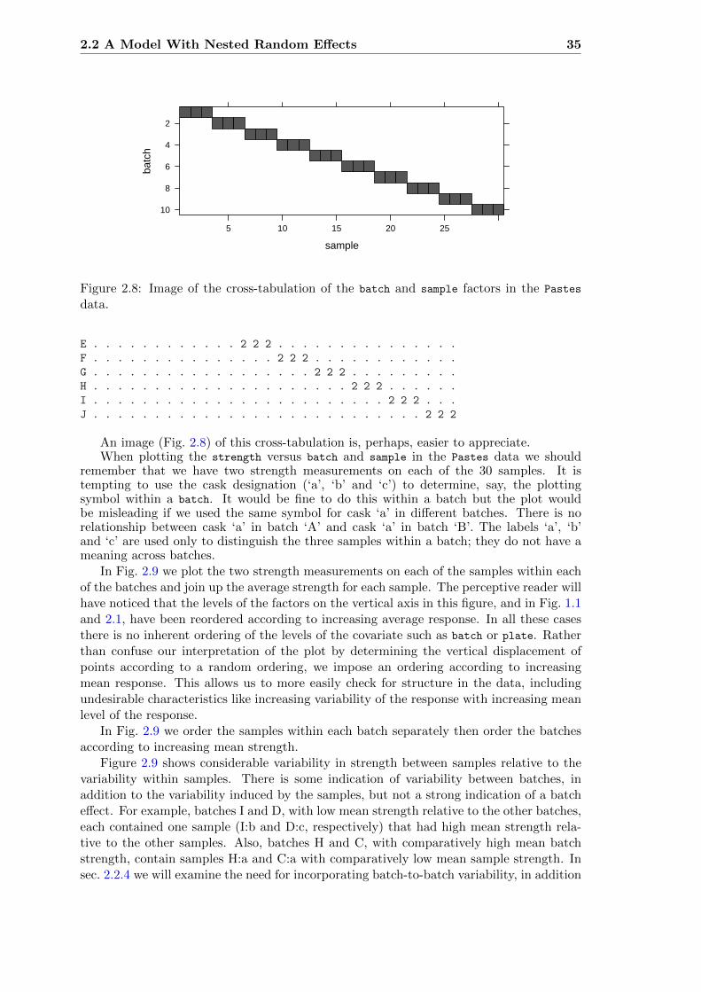
2.2 A Model With Nested Random Effects 35
sample
batc
h
2
4
6
8
10
5 10 15 20 25
Figure 2.8: Image of the cross-tabulation of the batch and sample factors in the Pastes
data.
E . . . . . . . . . . . . 2 2 2 . . . . . . . . . . . . . . .
F . . . . . . . . . . . . . . . 2 2 2 . . . . . . . . . . . .
G . . . . . . . . . . . . . . . . . . 2 2 2 . . . . . . . . .
H . . . . . . . . . . . . . . . . . . . . . 2 2 2 . . . . . .
I . . . . . . . . . . . . . . . . . . . . . . . . 2 2 2 . . .
J . . . . . . . . . . . . . . . . . . . . . . . . . . . 2 2 2
An image (Fig. 2.8) of this cross-tabulation is, perhaps, easier to appreciate.When plotting the strength versus batch and sample in the Pastes data we should
remember that we have two strength measurements on each of the 30 samples. It istempting to use the cask designation (‘a’, ‘b’ and ‘c’) to determine, say, the plottingsymbol within a batch. It would be fine to do this within a batch but the plot wouldbe misleading if we used the same symbol for cask ‘a’ in different batches. There is norelationship between cask ‘a’ in batch ‘A’ and cask ‘a’ in batch ‘B’. The labels ‘a’, ‘b’and ‘c’ are used only to distinguish the three samples within a batch; they do not have ameaning across batches.
In Fig. 2.9 we plot the two strength measurements on each of the samples within eachof the batches and join up the average strength for each sample. The perceptive reader willhave noticed that the levels of the factors on the vertical axis in this figure, and in Fig. 1.1and 2.1, have been reordered according to increasing average response. In all these casesthere is no inherent ordering of the levels of the covariate such as batch or plate. Ratherthan confuse our interpretation of the plot by determining the vertical displacement ofpoints according to a random ordering, we impose an ordering according to increasingmean response. This allows us to more easily check for structure in the data, includingundesirable characteristics like increasing variability of the response with increasing meanlevel of the response.
In Fig. 2.9 we order the samples within each batch separately then order the batchesaccording to increasing mean strength.
Figure 2.9 shows considerable variability in strength between samples relative to thevariability within samples. There is some indication of variability between batches, inaddition to the variability induced by the samples, but not a strong indication of a batcheffect. For example, batches I and D, with low mean strength relative to the other batches,each contained one sample (I:b and D:c, respectively) that had high mean strength rela-tive to the other samples. Also, batches H and C, with comparatively high mean batchstrength, contain samples H:a and C:a with comparatively low mean sample strength. Insec. 2.2.4 we will examine the need for incorporating batch-to-batch variability, in addition

36 Models With Multiple Random-effects Terms
Paste strength
Sam
ple
with
in b
atch
E:bE:aE:c
54 56 58 60 62 64 66
E
J:cJ:aJ:b
J
I:aI:cI:b
I
B:bB:cB:a
B
D:aD:bD:c
D
G:cG:bG:a
G
F:bF:cF:a
F
C:aC:bC:c
CA:bA:aA:c
A
H:aH:cH:b
H
Figure 2.9: Strength of paste preparations according to the batch and the sample withinthe batch. There were two strength measurements on each of the 30 samples; three sampleseach from 10 batches.
to sample-to-sample variability, in the statistical model.
Nested Factors
Because each level of sample occurs with one and only one level of batch we say that sampleis nested within batch. Some presentations of mixed-effects models, especially those relatedto multilevel modeling (Rasbash et al., 2000) or hierarchical linear models (Raudenbush &Bryk, 2002), leave the impression that one can only define random effects with respect tofactors that are nested. This is the origin of the terms “multilevel”, referring to multiple,nested levels of variability, and “hierarchical”, also invoking the concept of a hierarchy oflevels. To be fair, both those references do describe the use of models with random effectsassociated with non-nested factors, but such models tend to be treated as a special case.
The blurring of mixed-effects models with the concept of multiple, hierarchical levels ofvariation results in an unwarranted emphasis on “levels” when defining a model and leadsto considerable confusion. It is perfectly legitimate to define models having random effectsassociated with non-nested factors. The reasons for the emphasis on defining randomeffects with respect to nested factors only are that such cases do occur frequently in

2.2 A Model With Nested Random Effects 37
practice and that some of the computational methods for estimating the parameters inthe models can only be easily applied to nested factors.
This is not the case for the methods used in the lme4 package. Indeed there is nothingspecial done for models with random effects for nested factors. When random effects areassociated with multiple factors exactly the same computational methods are used whetherthe factors form a nested sequence or are partially crossed or are completely crossed.
There is, however, one aspect of nested grouping factors that we should emphasize,which is the possibility of a factor that is implicitly nested within another factor. Suppose,for example, that the sample factor was defined as having three levels instead of 30 withthe implicit assumption that sample is nested within batch. It may seem silly to try todistinguish 30 different batches with only three levels of a factor but, unfortunately, dataare frequently organized and presented like this, especially in text books. The cask factorin the Pastes data is exactly such an implicitly nested factor. If we cross-tabulate batch
and cask
> xtabs(~ cask + batch, Pastes)
batch
cask A B C D E F G H I J
a 2 2 2 2 2 2 2 2 2 2
b 2 2 2 2 2 2 2 2 2 2
c 2 2 2 2 2 2 2 2 2 2
we get the impression that the cask and batch factors are crossed, not nested. If we knowthat the cask should be considered as nested within the batch then we should create a newcategorical variable giving the batch-cask combination, which is exactly what the sample
factor is. A simple way to create such a factor is to use the interaction operator, ‘:’,on the factors. It is advisable, but not necessary, to apply factor to the result therebydropping unused levels of the interaction from the set of all possible levels of the factor.(An “unused level” is a combination that does not occur in the data.) A convenient codeidiom is
> Pastes$sample <- with(Pastes, factor(batch:cask))
or
> Pastes <- within(Pastes, sample <- factor(batch:cask))
In a small data set like Pastes we can quickly detect a factor being implicitly nestedwithin another factor and take appropriate action. In a large data set, with perhapshundreds of thousands of test scores for students in thousands of schools from hundredsof school districts, it is not always obvious if school identifiers are unique across the entiredata set or just within a district. If you are not sure, the safest thing to do is to create theinteraction factor, as shown above, so you can be confident that levels of the district:schoolinteraction do indeed correspond to unique schools.
2.2.2 Fitting a Model With Nested Random Effects
Fitting a model with simple, scalar random effects for nested factors is done in exactly thesame way as fitting a model with random effects for crossed grouping factors. We includerandom-effects terms for each factor, as in
> summary(fm04 <- lmer(strength ~ 1 + (1|sample) + (1|batch), Pastes, REML=FALSE))

38 Models With Multiple Random-effects Terms
Λ
10
20
30
10 20 30
Z'Z
10
20
30
10 20 30
L
10
20
30
10 20 30
Figure 2.10: Images of the relative covariance factor, Λ, the cross-product of the random-effects model matrix, ZTZ, and the sparse Cholesky factor, L, for model fm04.
Linear mixed model fit by maximum likelihood ['lmerMod']
Formula: strength ~ 1 + (1 | sample) + (1 | batch)
Data: Pastes
AIC BIC logLik deviance df.resid
256.0 264.4 -124.0 248.0 56
Scaled residuals:
Min 1Q Median 3Q Max
-1.48467 -0.52624 0.01215 0.46735 1.38918
Random effects:
Groups Name Variance Std.Dev.
sample (Intercept) 8.434 2.9041
batch (Intercept) 1.199 1.0951
Residual 0.678 0.8234
Number of obs: 60, groups: sample, 30; batch, 10
Fixed effects:
Estimate Std. Error t value
(Intercept) 60.0533 0.6421 93.52
Not only is the model specification similar for nested and crossed factors, the internalcalculations are performed according to the methods described in sec. 1.4.1 for each modeltype. Comparing the patterns in the matrices Λ, ZTZ and L for this model (Fig. 2.10) tothose in Fig. 2.4 shows that models with nested factors produce simple repeated structuresalong the diagonal of the sparse Cholesky factor, L, after reordering the random effects(we discuss this reordering later in sec. 5.4.1).This type of structure has the desirable property that there is no “fill-in” during calculationof the Cholesky factor. In other words, the number of non-zeros in L is the same as thenumber of non-zeros in the lower triangle of the matrix being factored, ΛTZTZΛ+I (which,because Λ is diagonal, has the same structure as ZTZ).
Fill-in of the Cholesky factor is not an important issue when we have a few dozenrandom effects, as we do here. It is an important issue when we have millions of randomeffects in complex configurations, as has been the case in some of the models that have

2.2 A Model With Nested Random Effects 39
sample
I:aE:bE:aD:aG:cB:bC:aI:c
D:bJ:c
H:aF:bJ:aE:cJ:b
G:bF:cB:cA:bB:aA:aA:cG:aC:bH:cF:aC:cI:b
D:cH:b
−5 0 5
batch
EJI
BDGFCAH
−3 −2 −1 0 1 2
Figure 2.11: 95% prediction intervals on the random effects for model fm04 fit to the Pastes
data.
been fit using lmer.
2.2.3 Assessing Parameter Estimates in Model fm04
The parameter estimates are: σ1 =2.904, the standard deviation of the random effects forsample; σ2 =1.095, the standard deviation of the random effects for batch; σ =0.823, thestandard deviation of the residual noise term; and β0 =60.053, the overall mean response,which is labeled (Intercept) in these models.
The estimated standard deviation for sample is nearly three times as large as that forbatch, which confirms what we saw in Fig. 2.9. Indeed our conclusion from Fig. 2.9 wasthat there may not be a significant batch-to-batch variability in addition to the sample-to-sample variability.
Plots of the prediction intervals of the random effects (Fig. 2.11)
confirm this impression in that all the prediction intervals for the random effects for batch
contain zero. Furthermore, the profile zeta plot (Fig. 2.12) shows that the even the 50%profile-based confidence interval on σ2 extends to zero.
Because there are several indications that σ2 could reasonably be zero, resulting in asimpler model incorporating random effects for batch only, we perform a statistical test ofthis hypothesis.

40 Models With Multiple Random-effects Terms
ζ
−2
−1
0
1
2
2.0 2.5 3.0 3.5 4.0 4.5
σ1
0 1 2 3
σ2
0.6 0.7 0.8 0.9 1.0 1.1 1.2
σ
58 59 60 61 62
(Intercept)
Figure 2.12: Profile zeta plots for the parameters in model fm04.
2.2.4 Testing H0 : σ2 = 0 Versus Ha : σ2 > 0
One of the many famous statements attributed to Albert Einstein is “Everything shouldbe made as simple as possible, but not simpler.” In statistical modeling this principal ofparsimony is embodied in hypothesis tests comparing two models, one of which containsthe other as a special case. Typically, one or more of the parameters in the more generalmodel, which we call the alternative hypothesis, is constrained in some way, resulting inthe restricted model, which we call the null hypothesis. Although we phrase the hypothesistest in terms of the parameter restriction, it is important to realize that we are comparingthe quality of fits obtained with two nested models. That is, we are not assessing param-eter values per se; we are comparing the model fit obtainable with some constraints onparameter values to that without the constraints.
Because the more general model, Ha, must provide a fit that is at least as good asthe restricted model, H0, our purpose is to determine whether the change in the qualityof the fit is sufficient to justify the greater complexity of model Ha. This comparison isoften reduced to a p-value, which is the probability of seeing a difference in the model fitsas large as we did, or even larger, when, in fact, H0 is adequate. Like all probabilities,a p-value must be between 0 and 1. When the p-value for a test is small (close to zero)we prefer the more complex model, saying that we “reject H0 in favor of Ha”. On theother hand, when the p-value is not small we “fail to reject H0”, arguing that there is anon-negligible probability that the observed difference in the model fits could reasonablybe the result of random chance, not the inherent superiority of the model Ha. Under thesecircumstances we prefer the simpler model, H0, according to the principal of parsimony.
These are the general principles of statistical hypothesis tests. To perform a test inpractice we must specify the criterion for comparing the model fits, the method for calcu-lating the p-value from an observed value of the criterion, and the standard by which wewill determine if the p-value is “small” or not. The criterion is called the test statistic, thep-value is calculated from a reference distribution for the test statistic, and the standardfor small p-values is called the level of the test.
In sec. 1.5 we referred to likelihood ratio tests (LRTs) for which the test statistic is thedifference in the deviance. That is, the LRT statistic is d0 − da where da is the deviancein the more general (Ha) model fit and d0 is the deviance in the constrained (H0) model.An approximate reference distribution for an LRT statistic is the χ2
ν distribution where

2.2 A Model With Nested Random Effects 41
ν, the degrees of freedom, is determined by the number of constraints imposed on theparameters of Ha to produce H0.
The restricted model fit
> summary(fm04a <- lmer(strength ~ 1 + (1|sample), Pastes, REML=FALSE))
Linear mixed model fit by maximum likelihood ['lmerMod']
Formula: strength ~ 1 + (1 | sample)
Data: Pastes
AIC BIC logLik deviance df.resid
254.4 260.7 -124.2 248.4 57
Scaled residuals:
Min 1Q Median 3Q Max
-1.49173 -0.54158 0.01509 0.46195 1.38824
Random effects:
Groups Name Variance Std.Dev.
sample (Intercept) 9.633 3.1037
Residual 0.678 0.8234
Number of obs: 60, groups: sample, 30
Fixed effects:
Estimate Std. Error t value
(Intercept) 60.0533 0.5765 104.2
is compared to model fm04 with the anova function
> anova(fm04a, fm04)
Data: Pastes
Models:
fm04a: strength ~ 1 + (1 | sample)
fm04: strength ~ 1 + (1 | sample) + (1 | batch)
npar AIC BIC logLik deviance Chisq Df Pr(>Chisq)
fm04a 3 254.40 260.69 -124.2 248.40
fm04 4 255.99 264.37 -124.0 247.99 0.4072 1 0.5234
which provides a p-value of 0.5234. Because typical standards for “small” p-values are5% or 1%, a p-value over 50% would not be considered significant at any reasonable level.
We do need to be cautious in quoting this p-value, however, because the parametervalue being tested, σ2 = 0, is on the boundary of set of possible values, σ2 ≥ 0, for thisparameter. The argument for using a χ2
1 distribution to calculate a p-value for the changein the deviance does not apply when the parameter value being tested is on the boundary.As shown in Pinheiro & Bates (2000, Sect. 2.5), the p-value from the χ2
1 distribution willbe “conservative” in the sense that it is larger than a simulation-based p-value would be.In the worst-case scenario the χ2-based p-value will be twice as large as it should be but,even if that were true, an effective p-value of 26% would not cause us to reject H0 in favorof Ha.
2.2.5 Assessing the Reduced Model, fm04a
The profile zeta plots for the remaining parameters in model fm04a (Fig. 2.13)are similar to the corresponding panels in Fig. 2.12, as confirmed by the numerical valuesof the confidence intervals.

42 Models With Multiple Random-effects Terms
ζ
−2
−1
0
1
2
2.5 3.0 3.5 4.0 4.5
σ1
0.6 0.7 0.8 0.9 1.0 1.1 1.2
σ
59 60 61
(Intercept)
Figure 2.13: Profile zeta plots for the parameters in model fm04a.
> confint(pr04)
2.5 % 97.5 %
.sig01 2.1579337 4.053589
.sig02 0.0000000 2.946591
.sigma 0.6520234 1.085448
(Intercept) 58.6636504 61.443016
> confint(pr04a)
2.5 % 97.5 %
.sig01 2.4306377 4.122011
.sigma 0.6520207 1.085448
(Intercept) 58.8861831 61.220484
The confidence intervals on log(σ) and β0 are similar for the two models. The confi-dence interval on σ1 is slightly wider in model fm04a than in fm04, because the variabilitythat is attributed to batch in fm04 is incorporated into the variability due to sample infm04a.
The patterns in the profile pairs plot (Fig. 2.14) for the reduced model fm04a are similarto those in Fig. A.1, the profile pairs plot for model fm01.

2.3 A Model With Partially Crossed Random Effects 43
Scatter Plot Matrix
.sig01
2.5 3.0 3.5 4.0 4.5 5.0
−3
−2
−1
0
.sigma
0.6
0.8
1.0
1.21.0 1.2
0 1 2 3
(Intercept)
58
59
60
61
62
0 1 2 3
Figure 2.14: Profile pairs plot for the parameters in model fm04a fit to the Pastes data.
2.3 A Model With Partially Crossed Random Effects
Especially in observational studies with multiple grouping factors, the configuration ofthe factors frequently ends up neither nested nor completely crossed. We describe suchsituations as having partially crossed grouping factors for the random effects.
Studies in education, in which test scores for students over time are also associatedwith teachers and schools, usually result in partially crossed grouping factors. If studentswith scores in multiple years have different teachers for the different years, the studentfactor cannot be nested within the teacher factor. Conversely, student and teacher factorsare not expected to be completely crossed. To have complete crossing of the student andteacher factors it would be necessary for each student to be observed with each teacher,which would be unusual. A longitudinal study of thousands of students with hundreds ofdifferent teachers inevitably ends up partially crossed.
In this section we consider an example with thousands of students and instructorswhere the response is the student’s evaluation of the instructor’s effectiveness. Thesedata, like those from most large observational studies, are quite unbalanced.
2.3.1 The InstEval Data
The InstEval data are from a special evaluation of lecturers by students at the SwissFederal Institute for Technology–Zurich (ETH–Zurich), to determine who should receivethe “best-liked professor” award. These data have been slightly simplified and identifying

44 Models With Multiple Random-effects Terms
labels have been removed, so as to preserve anonymity.The variables
> ## the default strict.width is 'no' for back-compatibility instead, we could also
> ## *globally* set strOptions(strict.width = 'cut') str(InstEval, strict.width = 'cut')
> str(InstEval)
'data.frame': 73421 obs. of 7 variables:
$ s : Factor w/ 2972 levels "1","2","3","4",..: 1 1 1 1 2 2 3 3 3 3 ...
$ d : Factor w/ 1128 levels "1","6","7","8",..: 525 560 832 1068 62 406 3 6 19 7..
$ studage: Ord.factor w/ 4 levels "2"<"4"<"6"<"8": 1 1 1 1 1 1 1 1 1 1 ...
$ lectage: Ord.factor w/ 6 levels "1"<"2"<"3"<"4"<..: 2 1 2 2 1 1 1 1 1 1 ...
$ service: Factor w/ 2 levels "0","1": 1 2 1 2 1 1 2 1 1 1 ...
$ dept : Factor w/ 14 levels "15","5","10",..: 14 5 14 12 2 2 13 3 3 3 ...
$ y : int 5 2 5 3 2 4 4 5 5 4 ...
have somewhat cryptic names. Factor s designates the student and d the instructor.The dept factor is the department for the course and service indicates whether the coursewas a service course taught to students from other departments.
Although the response, y, is on a scale of 1 to 5,
> xtabs(~ y, InstEval)
y
1 2 3 4 5
10186 12951 17609 16921 15754
it is sufficiently diffuse to warrant treating it as if it were a continuous response.At this point we will fit models that have random effects for student, instructor, and
department (or the dept:service combination) to these data. In the next chapter we willfit models incorporating fixed-effects for instructor and department to these data.
> summary(fm05 <- lmer(y ~ 1 + (1|s) + (1|d)+(1|dept:service),
+ InstEval, REML=FALSE))
Linear mixed model fit by maximum likelihood ['lmerMod']
Formula: y ~ 1 + (1 | s) + (1 | d) + (1 | dept:service)
Data: InstEval
AIC BIC logLik deviance df.resid
237663.3 237709.3 -118826.6 237653.3 73416
Scaled residuals:
Min 1Q Median 3Q Max
-2.9941 -0.7474 0.0400 0.7721 3.1124
Random effects:
Groups Name Variance Std.Dev.
s (Intercept) 0.10541 0.3247
d (Intercept) 0.26256 0.5124
dept:service (Intercept) 0.01213 0.1101
Residual 1.38495 1.1768
Number of obs: 73421, groups: s, 2972; d, 1128; dept:service, 28
Fixed effects:
Estimate Std. Error t value
(Intercept) 3.25521 0.02824 115.3

2.3 A Model With Partially Crossed Random Effects 45
dept:service
6:111:110:0
9:114:1
2:115:0
7:112:1
1:03:02:01:1
12:08:03:16:05:09:0
14:010:1
4:111:0
5:17:04:08:1
15:1
−0.3 −0.2 −0.1 0.0 0.1 0.2 0.3
Figure 2.15: 95% prediction intervals on the random effects for the dept:service factor inmodel fm05 fit to the InstEval data.
(Fitting this complex model to a moderately large data set takes less than two minuteson a modest laptop computer purchased in 2006. Although this is more time than requiredfor earlier model fits, it is a remarkably short time for fitting a model of this size andcomplexity. In some ways it is remarkable that such a model can be fit at all on such acomputer.)
All three estimated standard deviations of the random effects are less than σ, with σ3,the estimated standard deviation of the random effects for the dept:service interaction,less than one-tenth the estimated residual standard deviation.
> dotplot(rr4, strip = FALSE)
$`dept:service`
It is not surprising that zero is within all of the prediction intervals on the randomeffects for this factor (Fig. 2.15). In fact, zero is close to the middle of all these predictionintervals. However, the p-value for the LRT of H0 : σ3 = 0 versus Ha : σ3 > 0
> fm05a <- lmer(y ~ 1 + (1|s) + (1|d), InstEval, REML=FALSE)
> anova(fm05a,fm05)
Data: InstEval
Models:
fm05a: y ~ 1 + (1 | s) + (1 | d)
fm05: y ~ 1 + (1 | s) + (1 | d) + (1 | dept:service)
npar AIC BIC logLik deviance Chisq Df Pr(>Chisq)
fm05a 4 237786 237823 -118889 237778
fm05 5 237663 237709 -118827 237653 124.43 1 < 2.2e-16

46 Models With Multiple Random-effects Terms
Figure 2.16: Image of the sparse Cholesky factor, L, from model fm05
is highly significant. That is, we have very strong evidence that we should reject H0
in favor of Ha.The seeming inconsistency of these conclusions is due to the large sample size (n =
73421). When a model is fit to a very large sample even the most subtle of differencescan be highly “statistically significant”. The researcher or data analyst must then decideif these terms have practical significance, beyond the apparent statistical significance.
The large sample size also helps to assure that the parameters have good normalapproximations. We could profile this model fit but doing so would take a very longtime and, in this particular case, the analysts are more interested in a model that usesfixed-effects parameters for the instructors, which we will describe in the next chapter.
We could pursue other mixed-effects models here, such as using the dept factor andnot the dept:service interaction to define random effects, but we will revisit these datain the next chapter and follow up on some of these variations there.
2.3.2 Structure of L for model fm05
Before leaving this model we examine the sparse Cholesky factor, L, (Fig. 2.16), which isof size 4128× 4128. Even as a sparse matrix this factor requires a considerable amount ofmemory,
> object.size(getME(fm05,"L"))
8283432 bytes
> unclass(round(object.size(getME(fm05,"L"))/2^20, 3)) # size in megabytes

2.4 Chapter Summary 47
[1] 7.9
but as a triangular dense matrix it would require nearly 10 times as much. There are(4128× 4129)/2 elements on and below the diagonal, each of which would require 8 bytesof storage. A packed lower triangular array would require
> (8 * (4128 * 4129)/2)/2^20 # size in megabytes
[1] 65.01965
megabytes. The more commonly used full rectangular storage requires
> (8 * 4128^2)/2^20 # size in megabytes
[1] 130.0078
megabytes of storage.The number of nonzero elements in this matrix that must be updated for each evalu-
ation of the deviance is
> nnzero(as(getME(fm05,"L"), "sparseMatrix"))
[1] 566960
Comparing this to 8.522256× 10⁶, the number of elements that must be updated in adense Cholesky factor, we can see why the sparse Cholesky factor provides a much moreefficient evaluation of the profiled deviance function.
2.4 Chapter Summary
A simple, scalar random effects term in an lmer model formula is of the form (1|fac),where fac is an expression whose value is the grouping factor of the set of random effectsgenerated by this term. Typically, fac is simply the name of a factor, such as in the terms(1|sample) or (1|plate) in the examples in this chapter. However, the grouping factorcan be the value of an expression, such as (1|dept:service) in the last example.
Because simple, scalar random-effects terms can differ only in the description of thegrouping factor we refer to configurations such as crossed or nested as applying to theterms or to the random effects, although it is more accurate to refer to the configurationas applying to the grouping factors.
A model formula can include several such random effects terms. Because configurationssuch as nested or crossed or partially crossed grouping factors are a property of the data,the specification in the model formula does not depend on the configuration. We simplyinclude multiple random effects terms in the formula specifying the model.
One apparent exception to this rule occurs with implicitly nested factors, in which thelevels of one factor are only meaningful within a particular level of the other factor. Inthe Pastes data, levels of the cask factor are only meaningful within a particular level ofthe batch factor. A model formula of
strength ~ 1 + (1 | cask) + (1 | batch)
would result in a fitted model that did not appropriately reflect the sources of variabilityin the data. Following the simple rule that the factor should be defined so that distinct

48 Models With Multiple Random-effects Terms
experimental or observational units correspond to distinct levels of the factor will avoidsuch ambiguity.
For convenience, a model with multiple, nested random-effects terms can be specifiedas
strength ~ 1 + (1 | batch/cask)
which internally is re-expressed as
strength ~ 1 + (1 | batch) + (1 | batch:cask)
We will avoid terms of the form (1|batch/cask), preferring instead an explicit specifi-cation with simple, scalar terms based on unambiguous grouping factors.
The InstEval data, described in sec. 2.3.1, illustrate some of the characteristics of thereal data to which mixed-effects models are now fit. There is a large number of observa-tions associated with several grouping factors; two of which, student and instructor, havea large number of levels and are partially crossed. Such data are common in sociologicaland educational studies but until now it has been very difficult to fit models that appro-priately reflect such a structure. Much of the literature on mixed-effects models leaves theimpression that multiple random effects terms can only be associated with nested groupingfactors. The resulting emphasis on hierarchical or multilevel configurations is an artifactof the computational methods used to fit the models, not the models themselves.
The parameters of the models fit to small data sets have properties similar to thosefor the models in the previous chapter. That is, profile-based confidence intervals on thefixed-effects parameter, β0, are symmetric about the estimate but overdispersed relative tothose that would be calculated from a normal distribution and the logarithm of the residualstandard deviation, log(σ), has a good normal approximation. Profile-based confidenceintervals for the standard deviations of random effects (σ1, σ2, etc.) are symmetric on alogarithmic scale except for those that could be zero.
Another observation from the last example is that, for data sets with a very largenumber of observations, a term in a model may be “statistically significant” even whenits practical significance is questionable.
Exercises
These exercises use data sets from the MEMSS package for R. Recall that to access a particulardata set, you must either attach the package
> library(MEMSS)
or load just the one data set
> data(ergoStool, package = "MEMSS")
We begin with exercises using the ergoStool data from the MEMSS package. The analysisand graphics in these exercises is performed in Chap. 4. The purpose of these exercises isto see if you can use the material from this chapter to anticipate the results quoted in thenext chapter.

2.4 Chapter Summary 49
Check the documentation, the structure (str) and a summary of the ergoStool datafrom the MEMSS package. (If you are familiar with the Star Trek television series andmovies, you may want to speculate about what, exactly, the “Borg scale” is.) Use
> xtabs(~ Type + Subject, ergoStool)
to determine if these factors are nested, partially crossed or completely crossed. Is thisa replicated or an unreplicated design?
Create a plot, similar to Fig. 2.1, showing the effort by subject with lines connectingpoints corresponding to the same stool types. Order the levels of the Subject factor byincreasing average effort.
The experimenters are interested in comparing these specific stool types. In the nextchapter we will fit a model with fixed-effects for the Type factor and random effects forSubject, allowing us to perform comparisons of these specific types. At this point fit amodel with random effects for both Type and Subject. What are the relative sizes of theestimates of the standard deviations, σ1 (for Subject), σ2 (for Type) and σ (for the residualvariability)?
Refit the model using maximum likelihood. Check the parameter estimates and, inthe case of the fixed-effects parameter, β0, its standard error. In what ways have theparameter estimates changed? Which parameter estimates have not changed?
Profile the fitted model and construct 95% profile-based confidence intervals on theparameters. (Note that you will get the same profile object whether you start with theREML fit or the ML fit. There is a slight advantage in starting with the ML fit.) Is theconfidence interval on σ1 close to being symmetric about its estimate? Is the confidenceinterval on σ2 close to being symmetric about its estimate? Is the corresponding intervalon log(σ1) close to being symmetric about its estimate?
Create the profile zeta plot for this model. For which parameters are there good normalapproximations?
Create a profile pairs plot for this model. Comment on the shapes of the profile tracesin the transformed (ζ) scale and the shapes of the contours in the original scales of theparameters.
Create a plot of the 95% prediction intervals on the random effects for Type using
> dotplot(ranef(fm, which = "Type", condVar = TRUE), aspect = 0.2,
+ strip = FALSE)
(Substitute the name of your fitted model for fm in the call to ranef.) Is there a clearwinner among the stool types? (Assume that lower numbers on the Borg scale correspondto less effort).
Create a plot of the 95% prediction intervals on the random effects for Subject.

50 Models With Multiple Random-effects Terms
Check the documentation, the structure (str) and a summary of the Meat data fromthe MEMSS package. Use a cross-tabulation to discover whether Pair and Block are nested,partially crossed or completely crossed.
Use a cross-tabulation
> xtabs(~ Pair + Storage, Meat)
to determine whether Pair and Storage are nested, partially crossed or completelycrossed.
Fit a model of the score in the Meat data with random effects for Pair, Storage andBlock.
Plot the prediction intervals for each of the three sets of random effects.
Profile the parameters in this model. Create a profile zeta plot. Does including therandom effect for Block appear to be warranted. Does your conclusion from the profilezeta plot agree with your conclusion from examining the prediction intervals for the randomeffects for Block?
Refit the model without random effects for Block. Perform a likelihood ratio test ofH0 : σ3 = 0 versus Ha : σ3 > 0. Would you reject H0 in favor of Ha or fail to reject H0?Would you reach the same conclusion if you adjusted the p-value for the test by halvingit, to take into account the fact that 0 is on the boundary of the parameter region?
Profile the reduced model (i.e. the one without random effects for Block) and createprofile zeta and profile pairs plots. Can you explain the apparent interaction betweenlog(σ) and σ1? (This is a difficult question.)

Chapter 3
Models for Longitudinal Data
Longitudinal data consist of repeated measurements on the same subject (or some other“experimental unit”) taken over time. Generally we wish to characterize the time trendswithin subjects and between subjects. The data will always include the response, thetime covariate and the indicator of the subject on which the measurement has been made.If other covariates are recorded, say whether the subject is in the treatment group orthe control group, we may wish to relate the within- and between-subject trends to suchcovariates.
In this chapter we introduce graphical and statistical techniques for the analysis oflongitudinal data by applying them to a simple example.
3.1 The sleepstudy Data
Belenky et al. (2003) report on a study of the effects of sleep deprivation on reaction timefor a number of subjects chosen from a population of long-distance truck drivers. Thesesubjects were divided into groups that were allowed only a limited amount of sleep eachnight. We consider here the group of 18 subjects who were restricted to three hours of sleepper night for the first ten days of the trial. Each subject’s reaction time was measuredseveral times on each day of the trial.
> str(sleepstudy)
'data.frame': 180 obs. of 3 variables:
$ Reaction: num 250 259 251 321 357 ...
$ Days : num 0 1 2 3 4 5 6 7 8 9 ...
$ Subject : Factor w/ 18 levels "308","309","310",..: 1 1 1 1 1 1 1 1 1 1 ...
In this data frame, the response variable Reaction, is the average of the reactiontime measurements on a given subject for a given day. The two covariates are Days, thenumber of days of sleep deprivation, and Subject, the identifier of the subject on whichthe observation was made.
As recommended for any statistical analysis, we begin by plotting the data. The mostimportant relationship to plot for longitudinal data on multiple subjects is the trend ofthe response over time by subject, as shown in Fig. 3.1. This plot, in which the datafor different subjects are shown in separate panels with the axes held constant for all thepanels, allows for examination of the time-trends within subjects and for comparison ofthese patterns between subjects. Through the use of small panels in a repeating patternFig. 3.1 conveys a great deal of information, the individual time trends for 18 subjectsover 10 days — a total of 180 points — without being overly cluttered.
51

52 Models for Longitudinal Data
Days of sleep deprivation
Ave
rage
rea
ctio
n tim
e (m
s)
200
250
300
350
400
450
0 2 4 6 8
310 309
0 2 4 6 8
370 349
0 2 4 6 8
350 334
308 371 369 351 335
200
250
300
350
400
450
332
200
250
300
350
400
450
372
0 2 4 6 8
333 352
0 2 4 6 8
331 330
0 2 4 6 8
337
Figure 3.1: A lattice plot of the average reaction time versus number of days of sleepdeprivation by subject for the sleepstudy data. Each subject’s data are shown in a separatepanel, along with a simple linear regression line fit to the data in that panel. The panels areordered, from left to right along rows starting at the bottom row, by increasing interceptof these per-subject linear regression lines. The subject number is given in the strip abovethe panel.

3.1 The sleepstudy Data 53
3.1.1 Characteristics of the sleepstudy Data Plot
The principles of “Trellis graphics”, developed by Bill Cleveland and his coworkers atBell Labs and implemented in the lattice package for R by Deepayan Sarkar, have beenincorporated in this plot. As stated above, all the panels have the same vertical andhorizontal scales, allowing us to evaluate the pattern over time for each subject and alsoto compare patterns between subjects. The line drawn in each panel is a simple leastsquares line fit to the data in that panel only. It is provided to enhance our ability todiscern patterns in both the slope (the typical change in reaction time per day of sleepdeprivation for that particular subject) and the intercept (the average response time forthe subject when on their usual sleep pattern).
The aspect ratio of the panels (ratio of the height to the width) has been chosen,according to an algorithm described in Cleveland (1993), to facilitate comparison of slopes.The effect of choosing the aspect ratio in this way is to have the slopes of the lines on thepage distributed around ±45◦, thereby making it easier to detect systematic changes inslopes.
The panels have been ordered (from left to right starting at the bottom row) byincreasing intercept. Because the subject identifiers, shown in the strip above each panel,are unrelated to the response it would not be helpful to use the default ordering of thepanels, which is by increasing subject number. If we did so our perception of patterns in thedata would be confused by the, essentially random, ordering of the panels. Instead we usea characteristic of the data to determine the ordering of the panels, thereby enhancing ourability to compare across panels. For example, a question of interest to the experimentersis whether a subject’s rate of change in reaction time is related to the subject’s initialreaction time. If this were the case we would expect that the slopes would show anincreasing trend (or, less likely, a decreasing trend) in the left to right, bottom to topordering.
There is little evidence in Fig. 3.1 of such a systematic relationship between the sub-ject’s initial reaction time and their rate of change in reaction time per day of sleepdeprivation. We do see that for each subject, except 335, reaction time increases, more-or-less linearly, with days of sleep deprivation. However, there is considerable variationboth in the initial reaction time and in the daily rate of increase in reaction time. We canalso see that these data are balanced, both with respect to the number of observations oneach subject, and with respect to the times at which these observations were taken. Thiscan be confirmed by cross-tabulating Subject and Days.
> xtabs(~ Subject + Days, sleepstudy)
Days
Subject 0 1 2 3 4 5 6 7 8 9
308 1 1 1 1 1 1 1 1 1 1
309 1 1 1 1 1 1 1 1 1 1
310 1 1 1 1 1 1 1 1 1 1
330 1 1 1 1 1 1 1 1 1 1
331 1 1 1 1 1 1 1 1 1 1
332 1 1 1 1 1 1 1 1 1 1
333 1 1 1 1 1 1 1 1 1 1
334 1 1 1 1 1 1 1 1 1 1
335 1 1 1 1 1 1 1 1 1 1
337 1 1 1 1 1 1 1 1 1 1
349 1 1 1 1 1 1 1 1 1 1
350 1 1 1 1 1 1 1 1 1 1
351 1 1 1 1 1 1 1 1 1 1
352 1 1 1 1 1 1 1 1 1 1

54 Models for Longitudinal Data
369 1 1 1 1 1 1 1 1 1 1
370 1 1 1 1 1 1 1 1 1 1
371 1 1 1 1 1 1 1 1 1 1
372 1 1 1 1 1 1 1 1 1 1
In cases like this where there are several observations (10) per subject and a relativelysimple within-subject pattern (more-or-less linear) we may want to examine coefficientsfrom within-subject fixed-effects fits. However, because the subjects constitute a samplefrom the population of interest and we wish to draw conclusions about typical patterns inthe population and the subject-to-subject variability of these patterns, we will eventuallywant to fit mixed models and we begin by doing so. In sec. 3.4 we will compare estimatesfrom a mixed-effects model with those from the within-subject fixed-effects fits.
3.2 Mixed-effects Models For the sleepstudy Data
Based on our preliminary graphical exploration of these data, we fit a mixed-effects modelwith two fixed-effects parameters, the intercept and slope of the linear time trend for thepopulation, and two random effects for each subject. The random effects for a particularsubject are the deviations in intercept and slope of that subject’s time trend from thepopulation values.
We will fit two linear mixed models to these data. One model, fm06, allows for cor-relation (in the unconditional distribution) of the random effects for the same subject.That is, we allow for the possibility that, for example, subjects with higher initial reactiontimes may, on average, be more strongly affected by sleep deprivation. The second model,fm07, provides independent (again, in the unconditional distribution) random effects forintercept and slope for each subject.
3.2.1 A Model With Correlated Random Effects
The first model is fit as
> summary(fm06 <- lmer(Reaction ~ 1 + Days + (1 + Days|Subject),
+ sleepstudy, REML=FALSE))
Linear mixed model fit by maximum likelihood ['lmerMod']
Formula: Reaction ~ 1 + Days + (1 + Days | Subject)
Data: sleepstudy
AIC BIC logLik deviance df.resid
1763.9 1783.1 -876.0 1751.9 174
Scaled residuals:
Min 1Q Median 3Q Max
-3.9416 -0.4656 0.0289 0.4636 5.1793
Random effects:
Groups Name Variance Std.Dev. Corr
Subject (Intercept) 565.48 23.780
Days 32.68 5.717 0.08
Residual 654.95 25.592
Number of obs: 180, groups: Subject, 18
Fixed effects:

3.2 Mixed-effects Models For the sleepstudy Data 55
Λ
10
20
30
10 20 30
Σ
10
20
30
10 20 30
L
10
20
30
10 20 30
Figure 3.2: Images of Λ, Σ and L for model fm06
Estimate Std. Error t value
(Intercept) 251.405 6.632 37.907
Days 10.467 1.502 6.968
Correlation of Fixed Effects:
(Intr)
Days -0.138
From the display we see that this model incorporates both an intercept and a slope (withrespect to Days) in the fixed effects and in the random effects. Extracting the conditionalmodes of the random effects
> head(ranef(fm06)[["Subject"]])
(Intercept) Days
308 2.815789 9.0755068
309 -40.047855 -8.6441517
310 -38.432497 -5.5134706
330 22.831765 -4.6586649
331 21.549514 -2.9444450
332 8.815409 -0.2351823
confirms that these are vector-valued random effects. There are a total of q = 36 randomeffects, two for each of the 18 subjects.
The random effects section of the model display,
Subject (Intercept) 23.780
Days 5.717 0.08
Residual 25.592
Number of obs: 180, groups: Subject, 18
indicates that there will be a random effect for the intercept and a random effect for theslope with respect to Days at each level of Subject and, furthermore, the unconditionaldistribution of these random effects, B ∼ N (0,Σ), allows for correlation of the randomeffects for the same subject.
We can confirm the potential for correlation of random effects within subject in theimages of Λ, Σ and L for this model (Fig. 3.2). The matrix Λ has 18 triangular blocksof size 2 along the diagonal, generating 18 square, symmetric blocks of size 2 along the

56 Models for Longitudinal Data
diagonal of Σ. The 18 symmetric blocks on the diagonal of Σ are identical. Overall weestimate two standard deviations and a correlation for a vector-valued random effect ofsize 2, as shown in the model summary.
Often the variances and the covariance of random effects are quoted, rather than thestandard deviations and the correlation shown here. We have already seen that the vari-ance of a random effect is a poor scale on which to quote the estimate because confidenceintervals on the variance are so badly skewed. It is more sensible to assess the estimatesof the standard deviations of random effects or, possibly, the logarithms of the standarddeviations if we can be confident that 0 is outside the region of interest. We do display theestimates of the variances of the random effects but mostly so that the user can comparethese estimates to those from other software or for cases where an estimate of a varianceis expected (sometimes even required) to be given when reporting a mixed model fit.
We do not quote estimates of covariances of vector-valued random effects because thecovariance is a difficult scale to interpret, whereas a correlation has a fixed scale. Acorrelation must be between −1 and 1, allowing us to conclude that a correlation estimateclose to those extremes indicates that Σ is close to singular and the model is not wellformulated.
The estimates of the fixed effects parameters are β = (251.41, 10.467)T. These rep-resent a typical initial reaction time (i.e. without sleep deprivation) in the population ofabout 250 milliseconds, or 1/4 sec., and a typical increase in reaction time of a little morethan 10 milliseconds per day of sleep deprivation.
The estimated subject-to-subject variation in the intercept corresponds to a standarddeviation of about 25 ms. A 95% prediction interval on this random variable would beapproximately ±50 ms. Combining this range with a population estimated intercept of250 ms. indicates that we should not be surprised by intercepts as low as 200 ms. or ashigh as 300 ms. This range is consistent with the reference lines shown in Figure 3.1.
Similarly, the estimated subject-to-subject variation in the slope corresponds to astandard deviation of about 5.7 ms./day so we would not be surprised by slopes as lowas 10.5 − 2 · 5.7 = −0.9 ms./day or as high as 10.5 + 2 · 5.7 = 21.9 ms./day. Again, theconclusions from these rough, “back of the envelope” calculations are consistent with ourobservations from Fig. 3.1.
The estimated residual standard deviation is about 25 ms. leading us to expect ascatter around the fitted lines for each subject of up to ±50 ms. From Figure 3.1 we cansee that some subjects (309, 372 and 337) appear to have less variation than ±50 ms.about their within-subject fit but others (308, 332 and 331) may have more.
Finally, we see the estimated within-subject correlation of the random effect for theintercept and the random effect for the slope is very low, 0.081, confirming our impressionthat there is little evidence of a systematic relationship between these quantities. Inother words, observing a subject’s initial reaction time does not give us much informationfor predicting whether their reaction time will be strongly affected by each day of sleepdeprivation or not. It seems reasonable that we could get nearly as good a fit from a modelthat does not allow for correlation, which we describe next.
3.2.2 A Model With Uncorrelated Random Effects
In a model with uncorrelated random effects we have B ∼ N (0,Σ) where Σ is diagonal. Wehave seen models like this in previous chapters but those models had simple scalar randomeffects for all the grouping factors. Here we want to have a simple scalar random effect forSubject and a random effect for the slope with respect to Days, also indexed by Subject.We accomplish this by specifying two random-effects terms. The first, (1|Subject), is a

3.2 Mixed-effects Models For the sleepstudy Data 57
simple scalar term. The second has Days on the left hand side of the vertical bar.It may seem that the model formula we want should be
Reaction ~ 1 + Days + (1 | Subject) + (Days | Subject)
but it is not. Because the intercept is implicit in linear models, the second random effectsterm is equivalent to (1+Days|Subject) and will, by itself, produce correlated, vector-valued random effects.
We must suppress the implicit intercept in the second random-effects term, which wedo by writing it as (0+Days|Subject), read as “no intercept and Days by Subject”. Analternative expression for Days without an intercept by Subject is (Days - 1 | Subject).Using the first form we have
> summary(fm07 <- lmer(Reaction ~ 1 + Days + (1|Subject) +
+ (0+Days|Subject), sleepstudy, REML=FALSE))
Linear mixed model fit by maximum likelihood ['lmerMod']
Formula: Reaction ~ 1 + Days + (1 | Subject) + (0 + Days | Subject)
Data: sleepstudy
AIC BIC logLik deviance df.resid
1762 1778 -876 1752 175
Scaled residuals:
Min 1Q Median 3Q Max
-3.9535 -0.4673 0.0239 0.4625 5.1883
Random effects:
Groups Name Variance Std.Dev.
Subject (Intercept) 584.27 24.172
Subject.1 Days 33.63 5.799
Residual 653.12 25.556
Number of obs: 180, groups: Subject, 18
Fixed effects:
Estimate Std. Error t value
(Intercept) 251.405 6.708 37.48
Days 10.467 1.519 6.89
Correlation of Fixed Effects:
(Intr)
Days -0.194
As in model fm06, there are two random effects for each subject
> head(ranef(fm07)[["Subject"]])
(Intercept) Days
308 1.854750 9.2364126
309 -40.022659 -8.6174135
310 -38.723478 -5.4343288
330 23.903441 -4.8582077
331 22.396449 -3.1048565
332 9.052061 -0.2821684
but no correlation has been estimated

58 Models for Longitudinal Data
Λ
10
20
30
10 20 30
Σ
10
20
30
10 20 30
L
10
20
30
10 20 30
Figure 3.3: Images of Λ, the relative covariance factor, Σ, the variance-covariance matrixof the random effects, and L, the sparse Cholesky factor, in model fm07
10
20
30
10
20
30
Figure 3.4: Images of ZT for models fm06 (upper panel) and fm07 (lower panel)
Subject (Intercept) 24.172
Subject.1 Days 5.799
Residual 25.556
Number of obs: 180, groups: Subject, 18
The Subject factor is repeated in the “Groups” column because there were two distinctterms generating these random effects and these two terms had the same grouping factor.
Images of the matrices Λ, Σ and L (Fig. 3.3) show that Σ is indeed diagonal. Theorder of the random effects in Σ and Λ for model fm07 is different from the order in modelfm06. In model fm06 the two random effects for a particular subject were adjacent. Inmodel fm07 all the intercept random effects occur first then all the Days random effects.The sparse Cholesky decomposition, L, has the same form in both models because thefill-reducing permutation (described in sec. 5.4.1) calculated for model fm07 provides apost-ordering to group random effects with similar structure in Z.
Images of ZT for these two models (Fig. 3.4) shows that the columns of Z (rows of ZT)from one model are the same as those from the other model but in a different order.

3.2 Mixed-effects Models For the sleepstudy Data 59
3.2.3 Generating Z and Λ From Random-effects Terms
Let us consider these columns in more detail, starting with the columns of Z for modelfm07. The first 18 columns (rows in the bottom panel of Fig. 3.4) are the indicator columnsfor the Subject factor, as we would expect from the simple, scalar random-effects term(1|Subject). The pattern of zeros and non-zeros in the second group of 18 columns isdetermined by the indicators of the grouping factor, Subject, and the values of the non-zeros are determined by the Days covariate. In other words, these columns are formed bythe interaction of the numeric covariate, Days, and the categorical covariate, Subject.
The non-zero values in the model matrix Z for model fm06 are the same as those formodel fm06 but the columns are in a different order. Pairs of columns associated withthe same level of the grouping factor are adjacent. One way to think of the process ofgenerating these columns is to extend the idea of an interaction between a single covariateand the grouping factor to generating an “interaction” of a model matrix and the levels ofthe grouping factor. In other words, we begin with the two columns of the model matrixfor the expression 1 + Days and the 18 columns of indicators for the Subject factor. Theresult will have 36 columns that we regard as 18 adjacent pairs. The values within eachof these pairs of columns are the values of the 1 + Days columns, when the indicator is 1,otherwise they are zero.
We can now describe the general process of creating the model matrix, Z, and therelative covariance factor, Λ from the random-effects terms in the model formula. Eachrandom-effects term is of the form (expr|fac). The expression expr is evaluated as a linearmodel formula, producing a model matrix with s columns. The expression fac is evaluatedas a factor. Let k be the number of levels in this factor, after eliminating unused levels, ifany. The ith term generates siki columns in the model matrix, Z, and a diagonal blockof size siki in the relative covariance factor, Λ. The siki columns in Z have the pattern ofthe interaction of the si columns from the ith expr with the ki indicator columns for theith grouping factor fac. The diagonal block in Λ is itself block diagonal, consisting of kiblocks, each a lower triangular matrix of size si. In fact, these inner blocks are repetitionsof the same lower triangular si × si matrix. The i term contributes si(si + 1)/2 elementsto the variance-component parameter, θ, and these are the elements in the lower triangleof this si × si template matrix.
Note that when counting the columns in a model matrix we must take into accountthe implicit intercept term. For example, we could write the formula for model fm06 as
Reaction ~ Days + (Days | Subject)
realizing that the linear model expression, Days, actually generates two columns becauseof the implicit intercept.
Whether or not to include an explicit intercept term in a model formula is a matter ofpersonal taste. Many people prefer to write the intercept explicitly so as to emphasize therelationship between terms in the formula and coefficients or random effects in the model.Others omit these implicit terms so as to economize on the amount of typing required.Either approach can be used. The important point to remember is that the intercept mustbe explicitly suppressed when you don’t want it in a term.
Also, the intercept term must be explicit when it is the only term in the expression.That is, a simple, scalar random-effects term must be written as (1|fac) because a termlike (|fac) is not syntactically correct. However, we can omit the intercept from the fixed-effects part of the model formula if we have any random-effects terms. That is, we couldwrite the formula for model fm01 in Chap. 1 as

60 Models for Longitudinal Data
Yield ~ (1 | Batch)
or even
Yield ~ 1 | Batch
although omitting the parentheses around a random-effects term is risky. Becauseof operator precedence, the vertical bar operator, |, takes essentially everything in theexpression to the left of it as its first operand. It is advisable always to enclose such termsin parentheses so the scope of the operands to the | operator is clearly defined.
3.2.4 Comparing Models fm07 and fm06
Returning to models fm06 and fm07 for the sleepstudy data, it is easy to see that these arenested models because fm06 is reduced to fm07 by constraining the within-group correlationof random effects to be zero (which is equivalent to constraining the element below thediagonal in the 2× 2 lower triangular blocks of Λ in Fig. 3.2 to be zero).
We can use a likelihood ratio test to compare these fitted models.
> anova(fm07, fm06)
Data: sleepstudy
Models:
fm07: Reaction ~ 1 + Days + (1 | Subject) + (0 + Days | Subject)
fm06: Reaction ~ 1 + Days + (1 + Days | Subject)
npar AIC BIC logLik deviance Chisq Df Pr(>Chisq)
fm07 5 1762.0 1778.0 -876.00 1752.0
fm06 6 1763.9 1783.1 -875.97 1751.9 0.0639 1 0.8004
The value of the χ2 statistic, 0.0639, is very small, corresponding to a p-value of 0.80and indicating that the extra parameter in model fm06 relative to fm07 does not produce asignificantly better fit. By the principal of parsimony we prefer the reduced model, fm07.
This conclusion is consistent with the visual impression provided by Fig. 3.1. Theredoes not appear to be a strong relationship between a subject’s initial reaction time andthe extent to which his or her reaction time is affected by sleep deprivation.
In this likelihood ratio test the value of the parameter being tested, a correlation ofzero, is not on the boundary of the parameter space. We can be confident that the p-valuefrom the LRT adequately reflects the underlying situation.
(Note: It is possible to extend profiling to the correlation parameters and we will doso but that has not been done yet.)
3.3 Assessing the Precision of the Parameter Estimates
Plots of the profile ζ for the parameters in model fm07 (Fig. 3.5) show that confidenceintervals on σ1 and σ2 will be slightly skewed; those for log(σ) will be symmetric andwell-approximated by methods based on quantiles of the standard normal distributionand those for the fixed-effects parameters, β1 and β2 will be symmetric and slightly over-dispersed relative to the standard normal. For example, the 95% profile-based confidenceintervals are
> confint(pr07)

3.3 Assessing the Precision of the Parameter Estimates 61
ζ
−2
−1
0
1
2
20 30 40
σ1
4 6 8 10
σ2
22 24 26 28 30
σ
240 250 260 270
(Intercept)
6 8 10 12 14
Days
Figure 3.5: Profile zeta plot for each of the parameters in model fm07. The vertical linesare the endpoints of 50%, 80%, 90%, 95% and 99% profile-based confidence intervals foreach parameter.
2.5 % 97.5 %
.sig01 15.258647 37.786473
.sig02 3.964074 8.769159
.sigma 22.880555 28.787598
(Intercept) 237.572148 265.238062
Days 7.334067 13.600505
The profile pairs plot (Fig. 3.6)shows, for the most part, the usual patterns. First, consider the panels below the diagonal,which are on the (ζi, ζj) scales. The ζ pairs for log(σ) and β0, in the (4, 3) panel, and forlog(σ) and β1, in the (5, 3) panel, show the ideal pattern. The profile traces are straightand orthogonal, producing interpolated contours on the ζ scale that are concentric circlescentered at the origin. When mapped back to the scales of log(σ) and β0 or β1, in panels(3, 4) and (3, 5), these circles become slightly distorted, but this is only due to the moderatenonlinearity in the profile ζ plots for these parameters.
Examining the profile traces on the ζ scale for log(σ) versus σ1, the (3, 1) panel, orversus σ2, the (3, 2) panel, and for σ1 versus σ2, the (2, 1) panel, we see that close to theestimate the traces are orthogonal but as one variance component becomes small there isusually an increase in the others. In some sense the total variability in the response willbe partitioned across the contribution of the fixed effects and the variance components. Ineach of these panels the fixed-effects parameters are at their optimal values, conditionalon the values of the variance components, and the variance components must compensatefor each other. If one is made smaller then the others must become larger to compensate.
The patterns in the (4, 1) panel (σ1 versus β0, on the ζ scale) and the (5, 2) panel(σ2 versus β1, on the ζ scale) are what we have come to expect. As the fixed-effectsparameter is moved from its estimate, the standard deviation of the corresponding randomeffect increases to compensate. The (5, 1) and (4, 2) panels show that changing the valueof a fixed effect doesn’t change the estimate of the standard deviation of the randomeffects corresponding to the other fixed effect, which makes sense although the perfectorthogonality shown here will probably not be exhibited in models fit to unbalanced data.
In some ways the most interesting panels are those for the pair of fixed-effects param-eters: (5, 4) on the ζ scale and (4, 5) on the original scale. The traces are not orthogonal.

62 Models for Longitudinal Data
Scatter Plot Matrix
.sig01
10 20 30 40 50
−3
−2
−1
0
.sig02
4
6
8
108 10
0 1 2 3
.sigma
22
24
26
28
30 26 28 30
0 1 2 3
(Intercept)
230
240
250
260
270 250 260 270
0 1 2 3
Days
6
8
10
12
14
16
0 1 2 3
Figure 3.6: Profile pairs plot for the parameters in model fm07. The contour lines corre-spond to marginal 50%, 80%, 90%, 95% and 99% confidence regions based on the likelihoodratio. Panels below the diagonal represent the (ζi, ζj) parameters; those above the diagonalrepresent the original parameters.

3.4 Examining the Random Effects and Predictions 63
In fact the slopes of the traces at the origin of the (5, 4) (ζ scale) panel are the correlationof the fixed-effects estimators (−0.194 for this model) and its inverse. However, as wemove away from the origin on one of the traces in the (5, 4) panel it curves back towardthe horizontal axis (for the horizontal trace) or the vertical axis (for the vertical trace).In the ζ scale the individual contours are still concentric ellipses but their eccentricitychanges from contour to contour. The innermost contours have greater eccentricity thanthe outermost contours. That is, the outermost contours are more like circles than are theinnermost contours.
In a fixed-effects model the shapes of projections of deviance contours onto pairs offixed-effects parameters are consistent. In a fixed-effects model the profile traces in theoriginal scale will always be straight lines. For mixed models these traces can fail to belinear, as we see here, contradicting the widely-held belief that inferences for the fixed-effects parameters in linear mixed models, based on T or F distributions with suitablyadjusted degrees of freedom, will be completely accurate. The actual patterns of deviancecontours are more complex than that.
3.4 Examining the Random Effects and Predictions
The result of applying ranef to fitted linear mixed model is a list of data frames. Thecomponents of the list correspond to the grouping factors in the random-effects terms, notto the terms themselves. Model fm07 is the first model we have fit with more than oneterm for the same grouping factor where we can see the combination of random effectsfrom more than one term.
> str(rr1 <- ranef(fm07))
List of 1
$ Subject:'data.frame': 18 obs. of 2 variables:
..$ (Intercept): num [1:18] 1.85 -40.02 -38.72 23.9 22.4 ...
..$ Days : num [1:18] 9.24 -8.62 -5.43 -4.86 -3.1 ...
..- attr(*, "postVar")=List of 2
.. ..$ (Intercept): num [1, 1, 1:18] 146 146 146 146 146 ...
.. ..$ Days : num [1, 1, 1:18] 5.34 5.34 5.34 5.34 5.34 ...
- attr(*, "class")= chr "ranef.mer"
The plot method for "ranef.mer" objects produces one plot for each grouping factor.For scalar random effects the plot is a normal probability plot. For two-dimensionalrandom effects, including the case of two scalar terms for the same grouping factor, asin this model, the plot is a scatterplot. For three or more random effects per level ofthe grouping factor, the plot is a scatterplot matrix. The left hand panel in Fig. 3.7 wascreated with plot(ranef(fm07)).
The coef method for a fitted lmer model combines the fixed-effects estimates and theconditional modes of the random effects, whenever the column names of the random effectscorrespond to the names of coefficients. For model fm07 the fixed-effects coefficients are(Intercept) and Days and the columns of the random effects match these names. Thuswe can calculate some kind of per-subject “estimates” of the slope and intercept and plotthem, as in the right hand panel of Fig. 3.7. By comparing the two panels in Fig. 3.7 wecan see that the result of the coef method is simply the conditional modes of the randomeffects shifted by the coefficient estimates.
It is not entirely clear how we should interpret these values. They are a combinationof parameter estimates with the modal values of random variables and, as such, are ina type of “no man’s land” in the probability model. (In the Bayesian approach (Box

64 Models for Longitudinal Data
Days
(Int
erce
pt)
−40
−20
0
20
−10 −5 0 5 10
Days
(Int
erce
pt)
220
240
260
280
0 5 10 15 20
Figure 3.7: Plot of the conditional modes of the random effects for model fm07 (left panel)and the corresponding subject-specific coefficients (right panel)
& Tiao, 1973) to inference, however, both the parameters and the random effects arerandom variables and the interpretation of these values is straightforward.) Despite thedifficulties of interpretation in the probability model, these values are of interest becausethey determine the fitted response for each subject.
Comparison with an “all-fixed effects” linear model (‘lm(..)‘)
We can fit a separate regression line to each of the 18 subjects, in two different ways here:First, using one lm() with Subject × Days interaction and lmList() from package lme4
which calls lm() 18 times for each individual Subject, just using its 10 observations:First, the one lm() call on the full data set:
> (flm7 <- lm(Reaction ~ Days * Subject, sleepstudy))# "D * S": main effects + 2-way interactions
Call:
lm(formula = Reaction ~ Days * Subject, data = sleepstudy)
Coefficients:
(Intercept) Days Subject309 Subject310 Subject330
244.193 21.765 -39.138 -40.708 45.492
Subject331 Subject332 Subject333 Subject334 Subject335
41.546 20.059 30.826 -4.030 18.842
Subject337 Subject349 Subject350 Subject351 Subject352
45.911 -29.081 -18.358 16.954 32.179
Subject369 Subject370 Subject371 Subject372 Days:Subject309
10.775 -33.744 9.443 22.852 -19.503
Days:Subject310 Days:Subject330 Days:Subject331 Days:Subject332 Days:Subject333
-15.650 -18.757 -16.499 -12.198 -12.623
Days:Subject334 Days:Subject335 Days:Subject337 Days:Subject349 Days:Subject350
-9.512 -24.646 -2.739 -8.271 -2.261
Days:Subject351 Days:Subject352 Days:Subject369 Days:Subject370 Days:Subject371
-15.331 -8.198 -10.417 -3.709 -12.576

3.4 Examining the Random Effects and Predictions 65
Days:Subject372
-10.467
> ## dummy.coef(): *all* coefficients (inspite of contrasts giving "one coeff. less"):
> str(dcf7 <- dummy.coef(flm7))
List of 4
$ (Intercept) : Named num 244
..- attr(*, "names")= chr "(Intercept)"
$ Days : Named num 21.8
..- attr(*, "names")= chr "Days"
$ Subject : Named num [1:18] 0 -39.1 -40.7 45.5 41.5 ...
..- attr(*, "names")= chr [1:18] "308" "309" "310" "330" ...
$ Days:Subject: Named num [1:18] 0 -19.5 -15.6 -18.8 -16.5 ...
..- attr(*, "names")= chr [1:18] "308" "309" "310" "330" ...
- attr(*, "class")= chr "dummy_coef"
- attr(*, "matrix")= logi FALSE
> dfF <- as.data.frame(with(dcf7,
+ cbind(`(Intercept)` = `Subject`, Days = `Days:Subject`) +
+ cbind(`(Intercept)`, Days)[rep(1, length(Subject)),]))
> dfF
(Intercept) Days
308 244.1927 21.764702
309 205.0549 2.261785
310 203.4842 6.114899
330 289.6851 3.008073
331 285.7390 5.266019
332 264.2516 9.566768
333 275.0191 9.142045
334 240.1629 12.253141
335 263.0347 -2.881034
337 290.1041 19.025974
349 215.1118 13.493933
350 225.8346 19.504017
351 261.1470 6.433498
352 276.3721 13.566549
369 254.9681 11.348109
370 210.4491 18.056151
371 253.6360 9.188445
372 267.0448 11.298073
Secondly, here (and in all perfectly nested cases), this is the same as “one regressionfor each Subject”, i.e., using lmList()
> fmlmL <- lmList(Reaction ~ Days | Subject, sleepstudy)# pool = TRUE (is default)
> fmlmLs <- lmList(Reaction ~ Days | Subject, sleepstudy, pool = FALSE)
> df <- coef(fmlmL )
> dfs<- coef(fmlmLs) ; identical(df, dfs) ; rm(dfs)
[1] TRUE
> attributes(df) <- attributes(dfF) # <- for comparing, remove the extra "lmList" attributes of 'df'
> all.equal(df, dfF, tol = 1e-14)
[1] TRUE
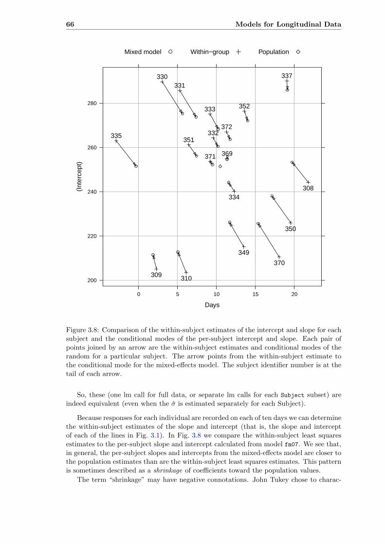
66 Models for Longitudinal Data
Days
(Int
erce
pt)
200
220
240
260
280
0 5 10 15 20
308
309 310
334
349
350
370
330331
332
333
335
337
351
352
369371
372
Mixed model Within−group Population
Figure 3.8: Comparison of the within-subject estimates of the intercept and slope for eachsubject and the conditional modes of the per-subject intercept and slope. Each pair ofpoints joined by an arrow are the within-subject estimates and conditional modes of therandom for a particular subject. The arrow points from the within-subject estimate tothe conditional mode for the mixed-effects model. The subject identifier number is at thetail of each arrow.
So, these (one lm call for full data, or separate lm calls for each Subject subset) areindeed equivalent (even when the σ is estimated separately for each Subject).
Because responses for each individual are recorded on each of ten days we can determinethe within-subject estimates of the slope and intercept (that is, the slope and interceptof each of the lines in Fig. 3.1). In Fig. 3.8 we compare the within-subject least squaresestimates to the per-subject slope and intercept calculated from model fm07. We see that,in general, the per-subject slopes and intercepts from the mixed-effects model are closer tothe population estimates than are the within-subject least squares estimates. This patternis sometimes described as a shrinkage of coefficients toward the population values.
The term “shrinkage” may have negative connotations. John Tukey chose to charac-
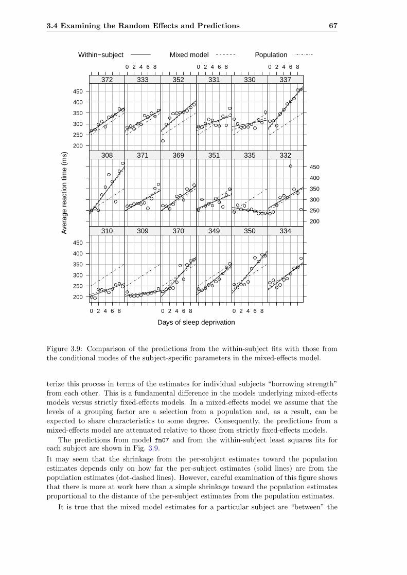
3.4 Examining the Random Effects and Predictions 67
Days of sleep deprivation
Ave
rage
rea
ctio
n tim
e (m
s)
200
250
300
350
400
450
0 2 4 6 8
310 309
0 2 4 6 8
370 349
0 2 4 6 8
350 334
308 371 369 351 335
200
250
300
350
400
450
332200
250
300
350
400
450
372
0 2 4 6 8
333 352
0 2 4 6 8
331 330
0 2 4 6 8
337
Within−subject Mixed model Population
Figure 3.9: Comparison of the predictions from the within-subject fits with those fromthe conditional modes of the subject-specific parameters in the mixed-effects model.
terize this process in terms of the estimates for individual subjects “borrowing strength”from each other. This is a fundamental difference in the models underlying mixed-effectsmodels versus strictly fixed-effects models. In a mixed-effects model we assume that thelevels of a grouping factor are a selection from a population and, as a result, can beexpected to share characteristics to some degree. Consequently, the predictions from amixed-effects model are attenuated relative to those from strictly fixed-effects models.
The predictions from model fm07 and from the within-subject least squares fits foreach subject are shown in Fig. 3.9.
It may seem that the shrinkage from the per-subject estimates toward the populationestimates depends only on how far the per-subject estimates (solid lines) are from thepopulation estimates (dot-dashed lines). However, careful examination of this figure showsthat there is more at work here than a simple shrinkage toward the population estimatesproportional to the distance of the per-subject estimates from the population estimates.
It is true that the mixed model estimates for a particular subject are “between” the

68 Models for Longitudinal Data
within-subject estimates and the population estimates, in the sense that the arrows inFig. 3.8 all point somewhat in the direction of the population estimate. However, theextent of the attenuation of the within-subject estimates toward the population estimatesis not simply related to the distance between those two sets of estimates. Consider thetwo panels, labeled 330 and 337, at the top right of Fig. 3.9. The within-subject estimatesfor 337 are quite unlike the population estimates but the mixed-model estimates are veryclose to these within-subject estimates. That is, the solid line and the dashed line in thatpanel are nearly coincident and both are a considerable distance from the dot-dashed line.For subject 330, however, the dashed line is more-or-less an average of the solid line andthe dot-dashed line, even though the solid and dot-dashed lines are not nearly as far apartas they are for subject 337.
The difference between these two cases is that the within-subject estimates for 337are very well determined. Even though this subject had an unusually large intercept andslope, the overall pattern of the responses is very close to a straight line. In contrast, theoverall pattern for 330 is not close to a straight line so the within-subject coefficients arenot well determined. The multiple R2 for the solid line in the 337 panel is 93.3% butin the 330 panel it is only 15.8%. The mixed model can pull the predictions in the 330panel, where the data are quite noisy, closer to the population line without increasing theresidual sum of squares substantially. When the within-subject coefficients are preciselyestimated, as in the 337 panel, very little shrinkage takes place.
We see from Fig. 3.9 that the mixed-effects model smooths out the between-subjectdifferences in the predictions by bringing them closer to a common set of predictions, butnot at the expense of dramatically increasing the sum of squared residuals. That is, thepredictions are determined so as to balance fidelity to the data, measured by the residualsum of squares, with simplicity of the model. The simplest model would use the sameprediction in each panel (the dot-dashed line) and the most complex model, based onlinear relationships in each panel, would correspond to the solid lines. The dashed linesare between these two extremes. We will return to this view of the predictions from mixedmodels balancing complexity versus fidelity in sec. 5.3, where we make the mathematicalnature of this balance explicit.
> dotplot(ranef(fm06,condVar=TRUE),scales = list(x = list(relation = "free")))[[1]]
We should also examine the prediction intervals on the random effects (Fig. 3.10) wherewe see that many prediction intervals overlap zero but there are several that do not. Inthis plot the subjects are ordered from bottom to top according to increasing conditionalmode of the random effect for (Intercept). The resulting pattern in the conditional modesof the random effect for Days reinforces our conclusion that the model fm07, which doesnot allow for correlation of the random effects for (Intercept) and Days, is suitable.
3.5 Chapter Summary
Problems
Check the structure of documentation, structure and a summary of the Orthodont dataset from the MEMSS package.(a) Create an xyplot of the distance versus age by Subject for the female subjects only.
You can use the optional argument subset = Sex == "Female" in the call to xyplot toachieve this. Use the optional argument type = c("g","p","r") to add reference linesto each panel.

3.5 Chapter Summary 69
Subject
309310370349350334335371308369351332372333352331330337
−60 −40 −20 0 20 40 60
(Intercept)
−15 −10 −5 0 5 10
Days
Figure 3.10: Prediction intervals on the random effects for model fm07.
(b) Enhance the plot by choosing an aspect ratio for which the typical slope of the refer-ence line is around 45o. You can set it manually (something like aspect = 4) or withan automatic specification (aspect = "xy"). Change the layout so the panels form onerow (layout = c(11,1)).
(c) Order the panels according to increasing response at age 8. This is achieved with theoptional argument index.cond which is a function of arguments x and y. In this caseyou could use index.cond = function(x,y) y[x == 8]. Add meaningful axis labels.Your final plot should be like
Age (yr)
Dis
tanc
e fr
om p
ituita
ry to
pte
rygo
max
illar
y fis
sure
(m
m)
16
18
20
22
24
26
28
89 11 13
F10
89 11 13
F06
89 11 13
F09
89 11 13
F03
89 11 13
F01
89 11 13
F02
89 11 13
F05
89 11 13
F07
89 11 13
F08
89 11 13
F04
89 11 13
F11
Figure 3.11: Distance versus age for the female subjects in the Orthodont data
(d) Fit a linear mixed model to the data for the females only with random effects forthe intercept and for the slope by subject, allowing for correlation of these random

70 Models for Longitudinal Data
effects within subject. Relate the fixed effects and the random effects’ variances andcovariances to the variability shown in the figure.
(e) Produce a “caterpillar plot” of the random effects for intercept and slope. Does theplot indicate correlated random effects?
(f) Consider what the Intercept coefficient and random effects represents. What willhappen if you center the ages by subtracting 8 (the baseline year) or 11 (the middleof the age range)?
(g) Repeat for the data from the male subjects.
Fit a model to both the female and the male subjects in the Orthodont data set, allowingfor differences by sex in the fixed-effects for intercept (probably with respect to the centeredage range) and slope.

Chapter 4
Building Linear Mixed Models
In the previous chapter we incorporated the time covariate of longitudinal data in both thefixed-effects terms and the random-effects terms of linear mixed models. In this chapterwe will extend the use of covariates, both numeric and categorical, in linear mixed modelsand discuss general approaches to building and assessing these models.
Statistical model building is still somewhat more of an art than a science and thereare many practical issues that we should bear in mind while engaged in it. We discusshow some of the optional arguments to the lmer function can be used to check for possibleproblems.
We begin with a discussion of categorical covariates and how they are incorporated inthe fixed-effects terms.
4.1 Incorporating categorical covariates with fixed levels
As we have seen in the earlier chapters, each random-effects term in a linear mixed modelis defined with respect to a grouping factor, which is a categorical covariate whose levelsare regarded as a sample from a population of possible levels. In some cases we may haveother categorical covariates with a fixed set of levels (such as gender, with fixed levelsmale and female) that we wish to incorporate into the model. Although incorporatingsuch covariates into the model formula is straightforward, the interpretation of coefficientsand the model’s structure can be subtle.
4.1.1 The Machines Data
Milliken & Johnson (2009, Table 23.1) discuss data from an experiment measuring pro-ductivity on a manufacturing task according to the type of machine used and the operator.No further details on the experiment are given and it is possible that these data, whichare available as Machines in the MEMSS package, were constructed for illustration and arenot observed data from an actual experiment.
> str(Machines)
'data.frame': 54 obs. of 3 variables:
$ Worker : Factor w/ 6 levels "1","2","3","4",..: 1 1 1 2 2 2 3 3 3 4 ...
$ Machine: Factor w/ 3 levels "A","B","C": 1 1 1 1 1 1 1 1 1 1 ...
$ score : num 52 52.8 53.1 51.8 52.8 53.1 60 60.2 58.4 51.1 ...
> xtabs(~ Machine + Worker, Machines)
71

72 Building Linear Mixed Models
Quality and productivity score
Wor
ker
6
2
4
1
5
3
45 50 55 60 65 70
● ●●
● ●●
●●●
● ●●
● ●●
●●●
A B C●
Figure 4.1: A quality and productivity score for each of six operators (the Worker factor)on each of three machine types.
Worker
Machine 1 2 3 4 5 6
A 3 3 3 3 3 3
B 3 3 3 3 3 3
C 3 3 3 3 3 3
The cross-tabulation shows that each of the six operators used each of the three ma-chines on three occasions producing replicate observations of the “subject-stimulus” com-binations. Although the operators represent a sample from the population of potentialoperators, the three machines are the specific machines of interest. That is, we regardthe levels of Machine as fixed levels and the levels of Worker as a random sample from apopulation. In other subject/stimulus studies we may regard the levels of the stimulus asa random sample from a population of stimuli.
We can see in Fig. 4.1
that, while the scores for each machine-operator combination are tightly clustered,there are considerable, apparently systematic, differences between machines and some-what smaller differences between operators. The pattern across operators for each of themachines is similar except for one unusual combination, operator 6 on machine B. Forthe other five operators the scores on machine A are less than those on machine B whichare less than those on Machine C but for operator 6 the scores on machine B are lessthan those on machine A. We expect our models to show a significant interaction betweenthe Worker and Machine factors because of this unusual pattern. As we will see, we canincorporate such an interaction into a linear mixed model in two different ways.
4.1.2 Comparing models with and without interactions
We fit and compare three models for these data: fm08 without interactions, fm09 withvector-valued random effects to allow for interactions, and fm10 with interactions incorpo-rated into a second simple scalar random-effects term.
> fm08 <- lmer(score ~ Machine + ( 1 |Worker), Machines, REML=FALSE)
> fm09 <- lmer(score ~ Machine + (Machine|Worker), Machines, REML=FALSE)

4.1 Incorporating categorical covariates with fixed levels 73
Warning in checkConv(attr(opt, "derivs"), opt$par, ctrl = control$checkConv, : Model
failed to converge with max|grad| = 0.00821788 (tol = 0.002, component 1)
> fm10 <- lmer(score ~ Machine + ( 1 |Worker) + (1|Machine:Worker),
+ Machines, REML=FALSE)
> anova(fm08, fm09, fm10)
Data: Machines
Models:
fm08: score ~ Machine + (1 | Worker)
fm10: score ~ Machine + (1 | Worker) + (1 | Machine:Worker)
fm09: score ~ Machine + (Machine | Worker)
Df AIC BIC logLik deviance Chisq Chi Df Pr(>Chisq)
fm08 5 303.70 313.65 -146.85 293.70
fm10 6 237.27 249.20 -112.64 225.27 68.4338 1 < 2e-16
fm09 10 236.42 256.31 -108.21 216.42 8.8516 4 0.06492
Notice that in the anova summary the order of the models has been rearranged ac-cording to the complexity of the models, as measured by the number of parameters tobe estimated. The simplest model, fm08, incorporates three fixed-effects parameters andtwo variance component parameters — a total of 5 parameters, the number displayed inthe column labeled Df. Model fm10, with scalar random effects for Worker and for theMachine:Worker combination incorporates one additional variance component for a totalof six parameters, while model fm09 adds five variance-component parameters to those infm08, for a total of 10 parameters.
In the comparison of models fm08 and fm10 (i.e. the line labeled fm10 in the anova table)we see that the additional parameter is highly significant. The change in the deviance of68.4338 (in the column labeled Chisq) at a cost of one additional parameter is huge; hencewe prefer the more complex model fm10. In the next line, which is the comparison ofthe more complex model fm09 to the simpler model fm10, the change in the deviance is8.8516 at a cost of 4 additional parameters with a p-value of 6.5%. In formal hypothesistests we establish a boundary, often chosen to be 5%, below which we regard the p-valueas providing “significant” evidence to prefer the more complex model and above whichthe results are regarded as representing an “insignificant” improvement. Such boundaries,while arbitrary, help us to assess the numerical results and here we prefer model fm10, ofintermediate complexity.
A display of this fitted model,
> fm10
Linear mixed model fit by maximum likelihood ['lmerMod']
Formula: score ~ Machine + (1 | Worker) + (1 | Machine:Worker)
Data: Machines
AIC BIC logLik deviance df.resid
237.2694 249.2034 -112.6347 225.2694 48
Random effects:
Groups Name Std.Dev.
Machine:Worker (Intercept) 3.3970
Worker (Intercept) 4.3645
Residual 0.9616
Number of obs: 54, groups: Machine:Worker, 18; Worker, 6
Fixed Effects:
(Intercept) MachineB MachineC
52.356 7.967 13.917
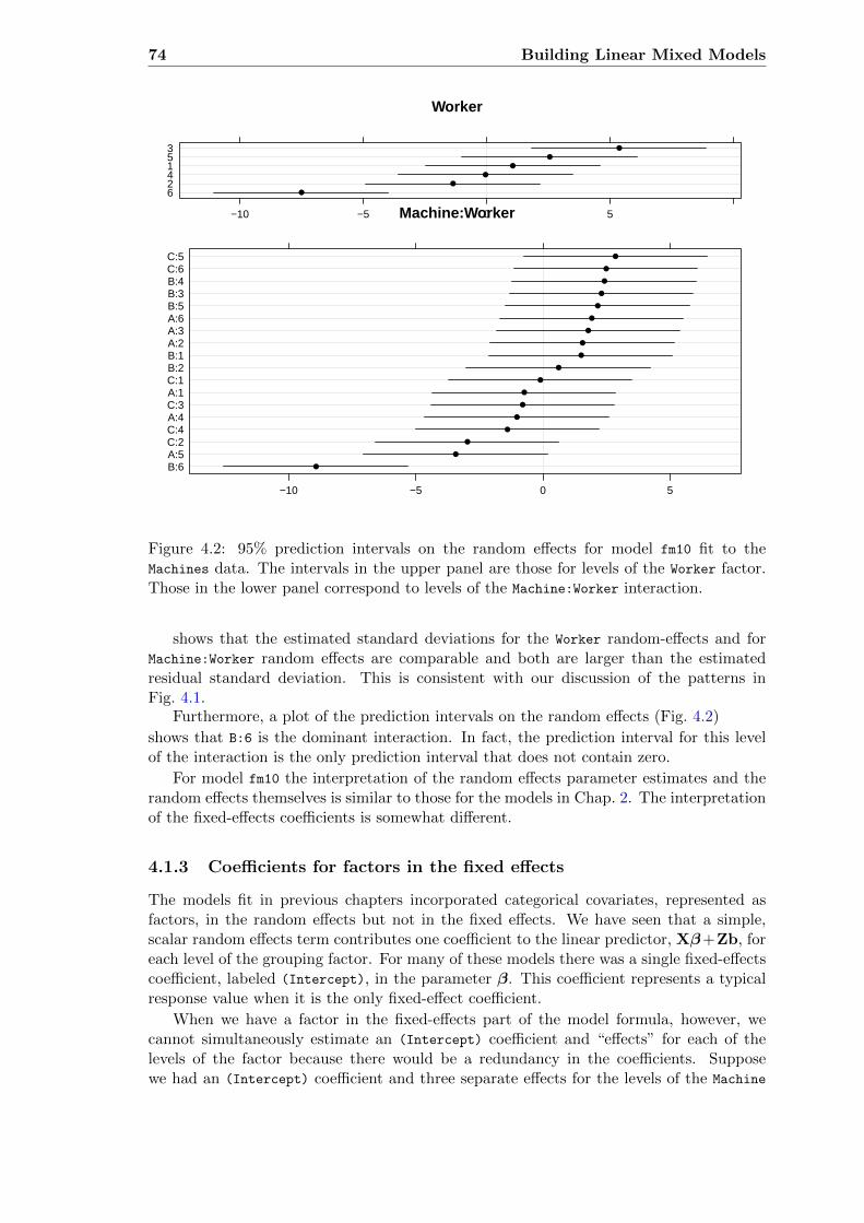
74 Building Linear Mixed Models
Machine:Worker
B:6A:5C:2C:4A:4C:3A:1C:1B:2B:1A:2A:3A:6B:5B:3B:4C:6C:5
−10 −5 0 5
●
●
●
●
●
●
●
●
●
●
●
●
●
●
●
●
●
●
Worker
624153
−10 −5 0 5
●
●
●
●
●
●
Figure 4.2: 95% prediction intervals on the random effects for model fm10 fit to theMachines data. The intervals in the upper panel are those for levels of the Worker factor.Those in the lower panel correspond to levels of the Machine:Worker interaction.
shows that the estimated standard deviations for the Worker random-effects and forMachine:Worker random effects are comparable and both are larger than the estimatedresidual standard deviation. This is consistent with our discussion of the patterns inFig. 4.1.
Furthermore, a plot of the prediction intervals on the random effects (Fig. 4.2)
shows that B:6 is the dominant interaction. In fact, the prediction interval for this levelof the interaction is the only prediction interval that does not contain zero.
For model fm10 the interpretation of the random effects parameter estimates and therandom effects themselves is similar to those for the models in Chap. 2. The interpretationof the fixed-effects coefficients is somewhat different.
4.1.3 Coefficients for factors in the fixed effects
The models fit in previous chapters incorporated categorical covariates, represented asfactors, in the random effects but not in the fixed effects. We have seen that a simple,scalar random effects term contributes one coefficient to the linear predictor, Xβ+Zb, foreach level of the grouping factor. For many of these models there was a single fixed-effectscoefficient, labeled (Intercept), in the parameter β. This coefficient represents a typicalresponse value when it is the only fixed-effect coefficient.
When we have a factor in the fixed-effects part of the model formula, however, wecannot simultaneously estimate an (Intercept) coefficient and “effects” for each of thelevels of the factor because there would be a redundancy in the coefficients. Supposewe had an (Intercept) coefficient and three separate effects for the levels of the Machine

4.1 Incorporating categorical covariates with fixed levels 75
factor. If we were to add a constant, say 2.6, to each of the effects coefficients and subtract2.6 from the (Intercept) we would generate the same set of fitted values and hence thesame likelihood. We would not be able to define a unique set of maximum likelihoodestimates, β.
In R this redundancy is removed by applying contrasts to the levels of a factor whenit is incorporated in the fixed-effects part of a linear predictor formula, and we can choosewhich contrasts are used when fitting a model. To show the effect of changing the contrastswe will refit model fm10 with different contrasts for the Machine factor and examine theestimated fixed effects. We can either extract the fixed-effects coefficient estimates bythemselves
> fixef(fm10)
(Intercept) MachineB MachineC
52.355556 7.966667 13.916667
or extract the coefficients and their standard errors and t ratios
> coef(summary(fm10))
Estimate Std. Error t value
(Intercept) 52.355556 2.269242 23.071830
MachineB 7.966667 1.987298 4.008794
MachineC 13.916667 1.987298 7.002809
for comparisons. To save on typing we will use update to fit the modified models. Recallthat update applied to a fitted model allows us to re-fit the model with changes that wespecify in subsequent arguments.
First let’s consider how the model changes if we suppress the intercept coefficient,which we can do by appending - 1 to the model formula. The update function allows usto do this by writing a model formula with dots indicating “what was there in the originalfit”. Thus
> (fm10a <- update(fm10, . ~ . - 1))
Linear mixed model fit by maximum likelihood ['lmerMod']
Formula: score ~ Machine + (1 | Worker) + (1 | Machine:Worker) - 1
Data: Machines
AIC BIC logLik deviance df.resid
237.2694 249.2034 -112.6347 225.2694 48
Random effects:
Groups Name Std.Dev.
Machine:Worker (Intercept) 3.3970
Worker (Intercept) 4.3645
Residual 0.9616
Number of obs: 54, groups: Machine:Worker, 18; Worker, 6
Fixed Effects:
MachineA MachineB MachineC
52.36 60.32 66.27
Notice that there are three fixed-effects coefficients in this model fit, just as there are inmodel fm10. All we have done by suppressing the intercept is to estimate a different set ofcoefficients in the fixed effects. The log-likelihood and the various statistics summarizingthe fit are the same — for example,

76 Building Linear Mixed Models
> AIC(fm10a,fm10)
df AIC
fm10a 6 237.2694
fm10 6 237.2694
Even the fitted values are the same
> all.equal(fitted(fm10a), fitted(fm10))
[1] TRUE
There are several things to note about model fm10a compared to model fm10. First,we can see that the —?!?— To see some of the approaches to removing this redun-dancy, including the defau —?!?— If we suppress the intercept we can estimate onecoefficient for each level of the factor
> coef(summary(update(fm10, . ~ . + 0)))
Estimate Std. Error t value
MachineA 52.35556 2.269242 23.07183
MachineB 60.32222 2.269242 26.58255
MachineC 66.27222 2.269242 29.20457
unless we impose additional estimability conditions on the coefficients.
—?!?— only one of the prediction intervals for the interaction that does not—?!?—
In both models fm09 and fm10 we incorporate the Machine factor —?!?— is in fitmodels having different configurations of simple, scalar random effects but always withthe same fixed-effects specification of an intercept, or overall mean response, only.
It is common in practice to have several fixed-effects terms involving one or morecovariates in the specification of a linear mixed model. Indeed, the purpose of fitting alinear mixed model is often to draw inferences about the effects of the covariates whileappropriately accounting for different sources of variability in the responses.
In this chapter we demonstrate how fixed-effects terms are incorporated in a linearmixed model and how inferences about the effects of the covariates are drawn from afitted linear mixed model.
4.2 Models for the ergoStool data
Problems 2.4 and 2.4 in Chap. 2 involve examining the structure of the ergoStool datafrom the MEMSS package
> str(ergoStool)
'data.frame': 36 obs. of 3 variables:
$ effort : num 12 15 12 10 10 14 13 12 7 14 ...
$ Type : Factor w/ 4 levels "T1","T2","T3",..: 1 2 3 4 1 2 3 4 1 2 ...
$ Subject: Factor w/ 9 levels "A","B","C","D",..: 1 1 1 1 2 2 2 2 3 3 ...
and plotting these data, as in Fig. 4.3.
These data are from an ergometrics experiment where nine subjects evaluated thedifficulty to arise from each of four types of stools. The measurements are on the scale

4.2 Models for the ergoStool data 77
Effort to arise (Borg scale)
H
E
D
I
F
C
G
A
B
8 10 12 14
●
●
●
●
●
●
●
●
●
T1 T2 T3 T4●
Figure 4.3: Subjective evaluation of the effort required to arise (on the Borg scale) by 9subjects, each of whom tried each of four types of stool.
of perceived exertion developed by the Swedish physician and researcher Gunnar Borg.Measurements on this scale are in the range 6-20 with lower values indicating less exertion.
From Fig. 4.3 we can see that all nine subjects rated type T1 or type T4 as requiringthe least exertion and rated type T2 as requiring the most exertion. Type T3 was perceivedas requiring comparatively little exertion by some subjects (H and E) and comparativelygreater exertion by others (F, C and G).
Problem 2.4 involves fitting and evaluating a model in which the effects of both theSubject and the Type factors are incorporated as random effects. Such a model may not beappropriate for these data where we wish to make inferences about these particular fourstool types. According to the distinction between fixed- and random-effects described insec. 1.1, if the levels of the Type factor are fixed and reproducible we generally incorporatethe factor in the fixed-effects part of the model.
Before doing so, let’s review the results of fitting a linear mixed model with randomeffects for both Subject and Type.
4.2.1 Random-effects for both Subject and Type
A model with random effects for both Subject and Type is fit in the same way that we fitsuch in Chap. 2,
> (fm16 <- lmer(effort ~ 1 + (1|Subject) + (1|Type), ergoStool, REML=FALSE))
Linear mixed model fit by maximum likelihood ['lmerMod']
Formula: effort ~ 1 + (1 | Subject) + (1 | Type)
Data: ergoStool
AIC BIC logLik deviance df.resid
144.0224 150.3564 -68.0112 136.0224 32
Random effects:
Groups Name Std.Dev.
Subject (Intercept) 1.305
Type (Intercept) 1.505
Residual 1.101
Number of obs: 36, groups: Subject, 9; Type, 4
Fixed Effects:

78 Building Linear Mixed Models
ζ
−2
−1
0
1
2
0.5 1.0 1.5 2.0 2.5 3.0
σ1
1 2 3 4 5
σ2
0.8 1.0 1.2 1.4 1.6
σ
8 10 12
(Intercept)
Figure 4.4: Profile zeta plot for the parameters in model fm16 fit to the ergoStool data
(Intercept)
10.25
from which we determine that the mean effort to arise, across stool types and acrosssubjects, is 10.250 on this scale, with standard deviations of 1.305 for the random-effectsfor the Subject factor and 1.505 for the Type factor.
One question we would want to address is whether there are “significant” differencesbetween stool types, taking into account the differences between subjects. We couldapproach this question by fitting a reduced model, without random effects for Type, andcomparing this fit to model fm16 using a likelihood-ratio test.
> fm16a <- lmer(effort ~ 1 + (1|Subject), ergoStool, REML=FALSE)
> anova(fm16a, fm16)
Data: ergoStool
Models:
fm16a: effort ~ 1 + (1 | Subject)
fm16: effort ~ 1 + (1 | Subject) + (1 | Type)
Df AIC BIC logLik deviance Chisq Chi Df Pr(>Chisq)
fm16a 3 164.15 168.90 -79.075 158.15
fm16 4 144.02 150.36 -68.011 136.02 22.128 1 2.551e-06
The p-value in this test is very small, indicating that the more complex model, fm16,which allows for differences in the effort to arise for the different stool types, provides asignificantly better fit to the observed data.
In sec. 2.2.4 we indicated that, because the constraint on the reduced model, σ2 = 0, ison the boundary of the parameter space, the p-value for this likelihood ratio test statisticcalculated using a χ2
1 reference distribution will be conservative. That is, the p-value onewould obtain by, say, simulation from the null distribution, would be even smaller thanthe p-value, 0.0000026, reported by this test, which is already very small.
Thus the evidence against the null hypothesis (H0 : σ2 = 0) and in favor of thealternative, richer model (Ha : σ2 > 0) is very strong.
Another way of addressing the question of whether it is reasonable for σ2 to be zero isto profile fm16 and examine profile zeta plots (Fig. 4.4)
and the corresponding profile pairs plot (Fig. 4.5).

4.2 Models for the ergoStool data 79
Scatter Plot Matrix
.sig01
0.5 1.0 1.5 2.0 2.5 3.0 3.5
−3
−2
−1
0
.sig02
2
4
6
86 8
0 1 2 3
.sigma
0.8
1.0
1.2
1.4
1.6
1.8 1.4 1.6 1.8
0 1 2 3
(Intercept)
6
8
10
12
14
0 1 2 3
Figure 4.5: Profile pairs plot for the parameters in model fm16 fit to the ergoStool data
We can see from the profile zeta plot (Fig. 4.4) that both σ1, the standard deviationof the Subject random effects, and, σ2, the standard deviation of the Type random effects,are safely non-zero. We also see that σ2 is very poorly determined. That is, a 95%profile-based confidence interval on this parameter, obtained as
> confint(pr16)[".sig02",]
2.5 % 97.5 %
0.7925051 3.7958573
is very wide. The upper end point of this 95% confidence interval, 3.796, is more thantwice as large as the estimate, σ2 = 1.505.
A plot
of the prediction intervals on the random effects for Type (Fig. 4.6) confirms the im-pression from Fig. 4.3 regarding the stool types. Type T2 requires the greatest effort andtype T1 requires the least effort. There is considerable overlap of the prediction intervals

80 Building Linear Mixed Models
Type
T1T4T3T2
−2 −1 0 1 2 3
●
●
●
●
Figure 4.6: 95% prediction intervals on the random effects for Type from model fm16 fit tothe ergoStool data
for types T1 and T4 and somewhat less overlap between types T4 and T3 and between typesT3 and T2.
In an analysis like this we begin by asking if there are any significant differences betweenthe stool types, which we answered for this model by testing the hypothesis H0 : σ2 = 0versus Ha : σ2 > 0. If we reject H0 in favor of Ha — that is, if we conclude that themore complex model including random effects for Type provides a significantly better fitthan the simpler model — then usually we want to follow up with the question, “Whichstool types are significantly different from each other?”. It is possible, though not easy,to formulate an answer to that question from a model fit such as fm16 in which the stooltypes are modeled with random effects, but it is more straightforward to address thatquestion when we model the stool types as fixed-effects parameters, which we do next.
4.2.2 Fixed Effects for Type, Random for Subject
To incorporate the Type factor in the fixed-effects parameters, instead of as a groupingfactor for random effects, we remove the random-effects term, (1|Type), and add Type tothe fixed-effects specification.
> (fm17 <- lmer(effort ~ 1 + Type + (1|Subject), ergoStool, REML = 0))
Linear mixed model fit by maximum likelihood ['lmerMod']
Formula: effort ~ 1 + Type + (1 | Subject)
Data: ergoStool
AIC BIC logLik deviance df.resid
134.1444 143.6456 -61.0722 122.1444 30
Random effects:
Groups Name Std.Dev.
Subject (Intercept) 1.256
Residual 1.037
Number of obs: 36, groups: Subject, 9
Fixed Effects:
(Intercept) TypeT2 TypeT3 TypeT4
8.5556 3.8889 2.2222 0.6667
It appears that the last three levels of the Type factor are now modeled as fixed-effects parameters, in addition to the (Intercept) parameter, whose estimate has de-creased markedly from that in model fm16. Furthermore, the estimates of the fixed-effectsparameters labeled TypeT2, TypeT3 and TypeT4, while positive, are very much smaller thanwould be indicated by the average responses for these types.
It turns out, of course, that the fixed-effects parameters generated by a factor covari-ate do not correspond to the overall mean and the effect for each level of the covariate.

4.2 Models for the ergoStool data 81
Although a model for an experiment such as this is sometimes written in a form like
yij = µ+ αi + bj + εij , i = 1, . . . , 4, j = 1, . . . 9 (4.1)
where i indexes the stool type and j indexes the subject, the parameters {µ, α1, α2, α3, α4},representing the overall mean and the effects of each of the stool types, are redundant.Given a set of estimates for these parameters we would not change the predictions from themodel if, for example, we added one to µ and subtracted one from all the α’s. In statisticalterminology we say that this set of parameters is not estimable unless we impose some otherconditions on them. The estimability condition
∑4i=1 αi = 0 is often used in introductory
texts.The approach taken in R is not based on redundant parameters that are subject to
estimability conditions. While this approach may initially seem reasonable, in complexmodels it quickly becomes unnecessarily complex to need to use constrained optimizationfor parameter estimation. Instead we incorporate the constraints into the parameters thatwe estimate. That is, we reduce the redundant set of parameters to an estimable set ofcontrasts between the levels of the factors.
The default contrasts generated for a factor
Although the particular set of contrasts used for a categorical factor can be controlledby the user, either as a global option for a session (see ?options) or by the optionalcontrasts argument available in most model-fitting functions, most users do not modifythe contrasts, preferring to leave them at the default setting, which is the “treatment”contrasts (contr.treatment) for an unordered factor and orthogonal polynomial contrasts(contr.poly) for an ordered factor. You can check the current global setting with
> getOption("contrasts")
unordered ordered
"contr.treatment" "contr.poly"
Because these were the contrasts in effect when model fm17 was fit, the particularcontrasts used for the Type factor, which has four levels, correspond to
> contr.treatment(4)
2 3 4
1 0 0 0
2 1 0 0
3 0 1 0
4 0 0 1
In this display the rows correspond to the levels of the Type factor and the columnscorrespond to the parameters labeled TypeT2, TypeT3 and TypeT4.
The values of Type in the data frame, whose first few rows are
> head(ergoStool)
effort Type Subject
1 12 T1 A
2 15 T2 A
3 12 T3 A
4 10 T4 A
5 10 T1 B
6 14 T2 B

82 Building Linear Mixed Models
combined with the contrasts produce the model matrix X, whose first few rows are
> head(model.matrix(fm17))
(Intercept) TypeT2 TypeT3 TypeT4
1 1 0 0 0
2 1 1 0 0
3 1 0 1 0
4 1 0 0 1
5 1 0 0 0
6 1 1 0 0
We see that the rows of X for observations on stool type T1 have zeros in the last threecolumns; the rows for observations on stool type T2 have a 1 in the second column andzeros in the last two columns, and so on. As before, the (Intercept) column is a columnof 1’s.
When we evaluate Xβ in the linear predictor expression, Xβ + Zb, we take the pelements of the fixed-effects parameter vector, β, whose estimate is
> fixef(fm17)
(Intercept) TypeT2 TypeT3 TypeT4
8.5555556 3.8888889 2.2222222 0.6666667
and the p elements of a row of the matrix X, multiply corresponding componentsand sum the resulting products. For example, the fixed-effects predictor for the firstobservation (stool type T1) will be
8.5556× 1 + 3.8889× 0 + 2.2222× 0 + 0.6667× 0 = 8.5556
and the fixed-effects predictor for the second observation (stool type T2) will be
8.5556× 1 + 3.8889× 1 + 2.2222× 0 + 0.6667× 0 = 12.4444
We see that the parameter labeled (Intercept) is actually the fixed-effects prediction forthe first level of Type (i.e. level T1) and the second parameter, labeled TypeT2, is thedifference between the fixed-effects prediction for the second level (T2) and the first level(T1) of the Type factor.
Similarly, the fixed-effects predictions for the T3 and T4 levels of Type are 8.5556 +2.2222 = 10.7778 and 8.5556 + 0.6667 = 9.2222, respectively, as can be verified from
> head(as.vector(model.matrix(fm17) %*% fixef(fm17)))
[1] 8.555556 12.444444 10.777778 9.222222 8.555556 12.444444
The fact that the parameter labeled TypeT2 is the difference between the fixed-effectsprediction for levels T2 and T1 of the Type factor is why we refer to the parameters as beinggenerated by contrasts. They are formed by contrasting the fixed-effects predictions forsome combination of the levels of the factor. In this case the contrast is between levels T2
and T1.In general, the parameters generated by the “treatment” contrasts (the default for
unordered factors) represent differences between the first level of the factor, which isincorporated into the (Intercept) parameter, and the subsequent levels. We say that thefirst level of the factor is the reference level and the others are characterized by their shiftrelative to this reference level.

4.2 Models for the ergoStool data 83
ζ
−2
−1
0
1
2
0.5 1.0 1.5 2.0 2.5
σ1
0.8 1.0 1.2 1.4
σ
7 8 9 10
(Intercept)
2.5 3.5 4.5
TypeT2
1.0 2.0 3.0
TypeT3
−0.5 0.5 1.5
TypeT4
Figure 4.7: Profile zeta plot for the parameters in model fm16 fit to the ergoStool data
Profiling the contrasts
Because some of the contrasts that are of interest to us correspond to fixed-effects param-eter values, we can profile the fitted model
(Fig. 4.7) and check, say, the confidence intervals on these parameters.
> confint(pr17, c("TypeT2", "TypeT3", "TypeT4"))
2.5 % 97.5 %
TypeT2 2.8953043 4.882473
TypeT3 1.2286377 3.215807
TypeT4 -0.3269179 1.660251
According to these intervals, and from what we see from Fig. 4.7, types T2 and T3 aresignificantly different from type T1 (the intervals do not contain zero) but type T4 is not(the confidence interval on this contrast contains zero).
However, this process must be modified in two ways to provide a suitable answer. Themost important modification is to take into account the fact that we are performing mul-tiple comparisons simultaneously. We describe what this means and how to accomodatefor it in the next subsection. The other problem is that this process only allows us toevaluate contrasts of the reference level, T1, with the other levels and the reference levelis essentially arbitrary. For completeness we should evaluate all six possible contrasts ofpairs of levels.
We can do this by refitting the model with a different reference level for the Type
factor and profiling the modified model fit. The relevel function allows us to change thereference level of a factor.
> pr17a <- profile(lmer(effort ~ 1 + Type + (1|Subject),
+ within(ergoStool, Type <- relevel(Type, "T2")),
+ REML=FALSE))
> pr17b <- profile(lmer(effort ~ 1 + Type + (1|Subject),
+ within(ergoStool, Type <- relevel(Type, "T3")),
+ REML=FALSE))
The other constrasts of interest are

84 Building Linear Mixed Models
> confint(pr17a, c("TypeT3", "TypeT4"))
2.5 % 97.5 %
TypeT3 -2.660251 -0.6730821
TypeT4 -4.215807 -2.2286377
> confint(pr17b, "TypeT4")
2.5 % 97.5 %
from which we would conclude that type T2 requires significantly greater effort thanany of the other types at the 5% level (because none of the 95% confidence intervals oncontrasts with T2 contain zero) and that types T3 and T4 are significantly different at the5% level.
However, we must take into account that we are performing multiple, simultaneouscomparisons of levels.
Multiple comparisons
In the technical definition of a confidence interval we regard the end points as being random(because they are calculated from the random variable which is the observed data) and thevalue of the parameter or the contrast of interest as being fixed (because it is determinedfrom the fixed, but unknown, values of the parameters). Thus we speak of the probabilitythat an interval covers the true parameter value rather than the probability that theparameter falls in the interval. The distinction may seem, and probably is, somewhatpedantic. We introduce it here simply to clarify the term “coverage probability” usedthroughout this section.
We have evaluated six possible pairwise comparisons of the four levels of the Type
factor. A 95% confidence interval on a particular contrast has, in theory, a 5% probabilityof failing to cover the true difference. That is, if the difference between two levels wasin fact zero, there would still be a 5% probability that a 95% confidence interval onthat contrast would not include zero. When we consider the coverage of the six intervalscontrasting all possible pairs of stool types we usually have in mind that there shouldbe a 95% probability of all six intervals covering the true, but unknown, differences ineffort for the stool types. That is, we think of the coverage probability as applying tothe simultaneous coverage of the family of intervals, not to the coverage of one specificinterval.
But the intervals calculated in the previous section were based on 95% coverage foreach specific interval. In the worst case scenario the family-wise coverage could be as lowas 1− 0.05 ∗ 6 = 0.70 or 70%. For factors with more than four levels there are even morepossible pairwise comparisons (for k levels there are k(k − 1)/2 possible pairs) and thisworst-case coverage probability is even further from the nominal level of 95%.
Several methods have been developed to compensate for multiple comparisons in theanalysis of linear models with fixed effects only. One of the simplest, although somewhatcoarse, compensations is the Bonferroni correction where the individual intervals are cho-sen to have a greater coverage probability in such a way that the “worst-case” probabilityis the desired level. With six comparisons to get a family-wise coverage probability of 95%the individual intervals are chosen to have coverage of
> (covrge <- 1 - 0.05/6)
[1] 0.9916667

4.2 Models for the ergoStool data 85
or a little more than 99%. We can specify this coverage level for the individual intervalsto ensure a family-wise coverage of at least 95%.
> rbind(confint(pr17, c("TypeT2","TypeT3","TypeT4"), covrge),
+ confint(pr17a, c("TypeT3","TypeT4"), covrge),
+ confint(pr17b, "TypeT4", covrge))
0.417 % 99.583 %
TypeT2 2.5109497 5.2668280
TypeT3 0.8442830 3.6001613
TypeT4 -0.7112726 2.0446058
TypeT3 -3.0446059 -0.2887275
TypeT4 -4.6001614 -1.8442831
We again reach the conclusion that the only pair of stool types for which zero is withinthe confidence interval on the difference in effects is the (T1,T4) pair but, for these intervals,the family-wise coverage of all six intervals is at least 95%.
There are other, perhaps more effective, techniques for adjusting intervals to take intoaccount multiple comparisons. The purpose of this section is to show that the profile-basedconfidence intervals can be extended to at least the Bonferroni correction.
The easiest way to apply other multiple comparison adjustment methods is to modelboth the Type and the Subject factors with fixed effects, which we do next.
4.2.3 Fixed Effects for Type and Subject
Even though the subjects in this study are chosen as representatives of a population,many statisticians would regard Subject as a blocking factor in the experiment and fit amodel with fixed-effects for both Type and Subject. A blocking factor is a known source ofvariability in the response. We are not interested in the effects of the levels of the blockingfactor—we only wish to accomodate for this source of variability when comparing levelsof the experimental factor, which is the Type factor in this example.
We will discuss the advantages and disadvantages of the fixed- versus random-effectschoice for the Subject factor at the end of this section. For the moment we proceed to fitthe fixed-effects model, for which we could use the lm function or the aov function. Thesetwo functions produce exactly the same model fit but the aov function returns an object ofclass "aov" which extends the class "lm", providing more options for examining the fittedmodel.
> summary(fm08 <- aov(effort ~ Subject + Type, ergoStool))
Df Sum Sq Mean Sq F value Pr(>F)
Subject 8 66.50 8.312 6.866 0.000106
Type 3 81.19 27.065 22.356 3.93e-07
Residuals 24 29.06 1.211
As seen above, the summary method for objects of class "aov" provides an analysis ofvariance table. The order in which the terms are listed in the model formula can affectthe results in this table, if the data are unbalanced, and we should be cautious to listthe terms in the model in the appropriate order, even for a balanced data set like theergoStool. The rule is that blocking factors should precede experimental factors becausethe contributions of the terms are assessed sequentially. Thus we read the rows in thistable as measuring the variability due to the Subject factor and due to the Type factorafter taking into account the Subject. We want to assess the experimental factor afterhaving removed the variability due to the blocking factor.

86 Building Linear Mixed Models
If desired we can assess individual coefficients by applying the summary method for"lm" objects, called summary.lm to this fitted model. For example, the coefficients table isavailable as
> coef(summary.lm(fm08))
Estimate Std. Error t value Pr(>|t|)
(Intercept) 1.055556e+01 0.6352554 1.661624e+01 1.146367e-14
SubjectB 6.005604e-15 0.7780258 7.719029e-15 1.000000e+00
SubjectC -1.500000e+00 0.7780258 -1.927957e+00 6.577394e-02
SubjectD -3.000000e+00 0.7780258 -3.855913e+00 7.577323e-04
SubjectE -3.750000e+00 0.7780258 -4.819892e+00 6.565314e-05
SubjectF -2.000000e+00 0.7780258 -2.570609e+00 1.678081e-02
SubjectG -1.500000e+00 0.7780258 -1.927957e+00 6.577394e-02
SubjectH -4.000000e+00 0.7780258 -5.141218e+00 2.907651e-05
SubjectI -2.250000e+00 0.7780258 -2.891935e+00 8.010522e-03
TypeT2 3.888889e+00 0.5186838 7.497610e+00 9.753420e-08
TypeT3 2.222222e+00 0.5186838 4.284348e+00 2.562927e-04
TypeT4 6.666667e-01 0.5186838 1.285304e+00 2.109512e-01
but often the individual coefficients are of less interest than the net effect of the vari-ability due to the levels of the factor, as shown in the analysis of variance table. Forexample, in the summary of the coefficients shown above the (Intercept) coefficient isthe predicted response for the reference subject (subject A) on the reference stool type(type T1). Other coefficients generated by the Subject term are the differences from thereference subject to other subjects. It is not clear why we would want to compare all theother subjects to subject A.
One of the multiple comparison methods that we can apply to fm08 is Tukey’s HonestSignificant Difference (HSD) method
> TukeyHSD(fm08, which = "Type")
Tukey multiple comparisons of means
95% family-wise confidence level
Fit: aov(formula = effort ~ Subject + Type, data = ergoStool)
$Type
diff lwr upr p adj
T2-T1 3.8888889 2.4580431 5.3197347 0.0000006
T3-T1 2.2222222 0.7913764 3.6530680 0.0013709
T4-T1 0.6666667 -0.7641791 2.0975125 0.5807508
T3-T2 -1.6666667 -3.0975125 -0.2358209 0.0182037
T4-T2 -3.2222222 -4.6530680 -1.7913764 0.0000115
T4-T3 -1.5555556 -2.9864013 -0.1247098 0.0295822
from which we reach essentially the same conclusions as before, although perhaps lessarduously.
4.2.4 Fixed Effects Versus Random Effects for Subject
These three analyses provoke the question of whether to use fixed-effects parameters orrandom effects for the Subject factor. That is, should Subject be treated as a blockingfactor or as a sample of levels from a population. If the sole purpose of the experiment isto rate the stool types relative to each other then it may be more convenient to consider

4.3 Covariates Affecting Mathematics Score Gain 87
Subject as a blocking factor in the experiment and incorporate it as the first term ina fixed-effects model for this completely balanced data set from a designed experiment.Strictly speaking, the inferences about the stool types that we would draw apply to theseparticular nine subjects only, not to a general population, but in practice it is not toomuch of a stretch to think of them as applying to a population unless we want to predictthe score that a general member of the population would give to a particular stool type.We can formulate the prediction but assessing the variability in the prediction is difficultwhen using fixed-effects models.
Random effects are preferred, perhaps even necessary, if we wish to make inferencesthat apply to the population of potential users. Also, when we have unbalanced dataor large samples, the flexibility of mixed models becomes important in stabilizing theestimation of parameters. The estimation of parameters in fixed-effects models by leastsquares is somewhat rigid. In theory it requires that the columns of the model matrix,X, are linearly independent. In practice, it is very difficult to determine if the columnsof a large model matrix are indeed linear independent or, equivalently, if the rank of Xis exactly p. The best we can do is determine if the condition number, κ, of X (the ratioof the largest to smallest singular values — see ?kappa) is sufficiently small to trust thenumerical linear algebra results. One way of thinking of κ is as a “magnification factor”for numerical perturbations. In the worst-case scenario, perturbations of relative size ε inthe elements of y results in perturbations of relative size κε in the coefficients β.
When the number of columns, p, of X is small the condition number tends to be small.
> kappa(fm08, exact = TRUE)
[1] 10.76924
However, when p is large the condition number of X tends to become very largeand evaluation of fixed-effects parameter estimates and their standard errors is an ill-conditioned problem.
Calculations involving the random effects model matrix, Z, are not as sensitive toill-conditioning. The numerical accuracy is determined by the condition number of thesparse Cholesky factor, Lθ, defined in (1.5) which is less than the condition number ofΛTθ ZTZΛθ, even when Λθ is singular.
> L16 <- as(getME(fm16, "L"), "Matrix")
> kappa(L16, exact = TRUE)
[1] 4.839807
The evaluation of Lθ is an example of regularization methods for solving ill-posedproblems or to prevent overfitting.
4.3 Covariates Affecting Mathematics Score Gain
West et al. (2007) provides comparisons of several different software systems for fittinglinear mixed models by fitting sample models to different data sets using each of thesesoftware systems. The lmer function from the lme4 package is not included in thesecomparisons because it was still being developed when that book was written.
In this section we will use lmer to fit models described in Chap. 4 of West et al. (2007)to data on the gain in mathematics scores for students in a selection of classrooms inseveral schools.

88 Building Linear Mixed Models
> str(classroom)
'data.frame': 1190 obs. of 11 variables:
$ sex : Factor w/ 2 levels "M","F": 2 1 2 1 1 2 1 1 2 1 ...
$ minority: Factor w/ 2 levels "N","Y": 2 2 2 2 2 2 2 2 2 2 ...
$ mathkind: int 448 460 511 449 425 450 452 443 422 480 ...
$ mathgain: int 32 109 56 83 53 65 51 66 88 -7 ...
$ ses : num 0.46 -0.27 -0.03 -0.38 -0.03 0.76 -0.03 0.2 0.64 0.13 ...
$ yearstea: num 1 1 1 2 2 2 2 2 2 2 ...
$ mathknow: num NA NA NA -0.11 -0.11 -0.11 -0.11 -0.11 -0.11 -0.11 ...
$ housepov: num 0.082 0.082 0.082 0.082 0.082 0.082 0.082 0.082 0.082 0.082 ...
$ mathprep: num 2 2 2 3.25 3.25 3.25 3.25 3.25 3.25 3.25 ...
$ classid : Factor w/ 312 levels "1","2","3","4",..: 160 160 160 217 217 217 217 217 ..
$ schoolid: Factor w/ 107 levels "1","2","3","4",..: 1 1 1 1 1 1 1 1 1 1 ...
The response modeled in Chap. 4 of West et al. (2007) is mathgain, the differencebetween a student’s mathematics score at the end of grade one and at the end of kinder-garten. To allow comparisons with the results in West et al. (2007) we will use thatresponse in this section.
There is one observation per student. In the terminology of the multilevel modelingliterature the levels of variability correspond to student (level 1), classroom (level 2) andschool (level 3) with the assumption that classroom is nested within school. The conceptof “levels” can only be applied to models and data sets in which the grouping factors ofthe random effects form a nested sequence. In crossed or partially crossed configurationsthere are no clearly defined levels.
At this point we should check if there is implicit nesting. That is, are the levels ofthe classid factor nested within schoolid factor. We could simply create the interactionfactor to avoid the possibility of implicit nesting but it saves a bit of trouble if we checkbefore doing so
> with(classroom, isNested(classid, schoolid))
[1] TRUE
A model with simple, scalar random effects and without any fixed-effects terms (otherthan the implicit intercept) is called the “unconditional model” in the multilevel modelingliterature. We fit it as
> (fm09 <- lmer(mathgain ~ (1|classid) + (1|schoolid), classroom))
Linear mixed model fit by REML ['lmerMod']
Formula: mathgain ~ (1 | classid) + (1 | schoolid)
Data: classroom
REML criterion at convergence: 11768.76
Random effects:
Groups Name Std.Dev.
classid (Intercept) 9.961
schoolid (Intercept) 8.804
Residual 32.066
Number of obs: 1190, groups: classid, 312; schoolid, 107
Fixed Effects:
(Intercept)
57.43
The results from this model fit using the REML criterion can be compared to Table4.6 (page 156) of West et al. (2007).

4.3 Covariates Affecting Mathematics Score Gain 89
Gain in Mathematics score from kindergarten to first grade
Cla
ssro
om w
ithin
sch
ool
8277136287
28
0 50 100 150 200
● ●●●
● ●●●●
● ●● ●● ●●● ● ●● ●●
● ●● ● ●
76
214266205226236
●● ●● ●● ●● ●
●
● ●●●
●● ●●●99
3022049
25181
● ●●
● ●●● ● ●
● ● ●● ●● ● ●●●●
●● ●●●●●
12
264304
80120209
● ●●● ●●●● ●●● ●● ●
● ●
● ●● ●● ● ●●● ●●
71
18666
15784
196
●● ●● ● ●
●
● ●● ●
● ● ●● ●●
●●●
85
69240133
7119 ●●
●● ●
● ●
●●●● ● ●
46
8832
10026
229●●● ● ●●● ●● ●
● ● ●●●●
●
● ● ●●●
33
272250171
3640
●●●●
●● ●
●
57
260119
8592
5 ●
●● ● ●● ●●●
●
● ●●
15
787
216177
10
●
●●
●
●●●
● ●17
57263271298244
● ●● ●
●
●● ●● ●●
●● ● ● ●
68311261152
83146
●● ● ● ●● ●
● ●●
●● ●● ●●
●●●
70
Figure 4.8: Comparative dotplots of gain in the mathematics scores in classrooms withinschools.
It seems that the housepov value is a property of the school. We can check this byconsidering the number of unique combinations of housepov and schoolid and comparingthat to the number of levels of schoolid. For safety we check the number of levels offactor(schoolid) in case there are unused levels in schoolid.
> with(classroom, length(levels(factor(schoolid))))
[1] 107
> nrow(unique(subset(classroom, select = c(schoolid, housepov))))
[1] 107
In some formulations of multilevel models or hierarchical linear models it is importantto associate covariates with different levels in the hierarchy.

90 Building Linear Mixed Models
ζ
−2
−1
0
1
2
4 6 8 10 12
σ1
6 8 10 12
σ2
26 27 28
σ
70 75 80
(Intercept)
−0.52 −0.48 −0.44
I(mathkind − 450)−4 −2 0 2
sexF
−14 −10 −6 −4 −2
minorityY
2 4 6 8
ses
−30 −10 0 10
−2
−1
0
1
2
housepov
Figure 4.9: Profile plot of the parameters in model fm4.
> (fm14 <- lmer(mathgain ~ 1 + I(mathkind-450) + sex + minority + ses
+ + housepov + (1|classid) + (1|schoolid), classroom))
Linear mixed model fit by REML ['lmerMod']
Formula: mathgain ~ 1 + I(mathkind - 450) + sex + minority + ses + housepov +
(1 | classid) + (1 | schoolid)
Data: classroom
REML criterion at convergence: 11378.06
Random effects:
Groups Name Std.Dev.
classid (Intercept) 9.031
schoolid (Intercept) 8.818
Residual 27.100
Number of obs: 1190, groups: classid, 312; schoolid, 107
Fixed Effects:
(Intercept) I(mathkind - 450) sexF minorityY
73.1708 -0.4709 -1.2346 -7.7559
ses housepov
5.2397 -11.4392
A profile plot of the parameters in model fm14 is shown in Fig. 4.9.
4.4 Rat Brain example
> ftable(xtabs(activate ~ animal + treatment + region, ratbrain))
region BST LS VDB
animal treatment

4.4 Rat Brain example 91
activate
BST
LS
VDB
200 300 400 500 600 700
●
●
●
Bas
al
BST
LS
VDB
●
●
●C
arba
chol
R100797R100997R110597R111097R111397
●
Figure 4.10: Activation of brain regions in rats
R100797 Basal 458.16 245.04 237.42
Carbachol 664.72 587.10 726.96
R100997 Basal 479.81 261.19 195.51
Carbachol 515.29 437.56 604.29
R110597 Basal 462.79 278.33 262.05
Carbachol 589.25 493.93 621.07
R111097 Basal 366.19 199.31 187.11
Carbachol 371.71 302.02 449.70
R111397 Basal 375.58 204.85 179.38
Carbachol 492.58 355.74 459.58
Description of the Rat Brain data should go here.

92 Building Linear Mixed Models

Chapter 5
Computational Methods forMixed Models
In this chapter we describe some of the details of the computational methods for fittinglinear mixed models, as implemented in the lme4 package, and the theoretical developmentbehind these methods. We also provide the basis for later generalizations to models fornon-Gaussian responses and to models in which the relationship between the conditionalmean, µ, and the linear predictor, γ = Xβ+Zb = ZΛθu+Xβ, is a nonlinear relationship.
This material is directed at those readers who wish to follow the theory and methodol-ogy of linear mixed models and how both can be extended to other forms of mixed models.Readers who are less interested in the “how” and the “why” of fitting mixed models thanin the results themselves should not feel obligated to master these details.
We begin by reviewing the definition of linear mixed-effects models and some of thebasics of the computational methods, as given in sec. 1.1.
5.1 Definitions and Basic Results
As described in sec. 1.1, a linear mixed-effects model is based on two vector-valued randomvariables: the q-dimensional vector of random effects, B, and the n-dimensional responsevector, Y . Equation (1.1) defines the unconditional distribution of B and the conditionaldistribution of Y , given B = b, as multivariate Gaussian distributions of the form
(Y |B = b) ∼ N (Xβ + Zb, σ2I)
B ∼ N (0,Σθ).
The q × q, symmetric, variance-covariance matrix, Var(B) = Σθ, depends on thevariance-component parameter vector, θ, and is positive semidefinite, which means that
bTΣθb ≥ 0, ∀b 6= 0. (5.1)
(The symbol ∀ denotes “for all”.) The fact that Σθ is positive semidefinite does notguarantee that Σ−1θ exists. We would need a stronger property, bTΣθb > 0, ∀b 6= 0,called positive definiteness, to ensure that Σ−1θ exists.
Many computational formulas for linear mixed models are written in terms of Σ−1θ .Such formulas will become unstable as Σθ approaches singularity. And it can do so. It isa fact that singular (i.e. non-invertible) Σθ can and do occur in practice, as we have seenin some of the examples in earlier chapters. Moreover, during the course of the numericaloptimization by which the parameter estimates are determined, it is frequently the case
93

94 Computational Methods for Mixed Models
that the deviance or the REML criterion will need to be evaluated at values of θ thatproduce a singular Σθ. Because of this we will take care to use computational methodsthat can be applied even when Σθ is singular and are stable as Σθ approaches singularity.
As defined in (1.2) a relative covariance factor, Λθ, is any matrix that satisfies
Σθ = σ2ΛθΛTθ .
According to this definition, Σ depends on both σ and θ and we should write it as Σσ,θ.However, we will blur that distinction and continue to write Var(B) = Σθ. Anothertechnicality is that the common scale parameter, σ, can, in theory, be zero. We will showthat in practice the only way for its estimate, σ, to be zero is for the fitted values fromthe fixed-effects only, Xβ, to be exactly equal to the observed data. This occurs onlywith data that have been (incorrectly) simulated without error. In practice we can safelyassume that σ > 0. However, Λθ, like Σθ, can be singular.
Our computational methods are based on Λθ and do not require evaluation of Σθ. Infact, Σθ is explicitly evaluated only at the converged parameter estimates.
The spherical random effects, U ∼ N (0, σ2Iq), determine B as
B = ΛθU . (5.2)
Although it may seem more intuitive to write U as a linear transformation of B, we cannotdo that when Λθ is singular, which is why (5.2) is in the form shown.
We can easily verify that (5.2) provides the desired distribution for B. As a lineartransformation of a multivariate Gaussian random variable, B will also be multivariateGaussian. Its mean and variance-covariance matrix are straightforward to evaluate,
E[B] = ΛθE[U ] = Λθ0 = 0 (5.3)
and
Var(B) = E[(B − E[B])(B − E[B])T
]= E
[BBT
]= E
[Λθ UUTΛT
θ
]= Λθ E[UUT]ΛT
θ = Λθ Var(U)ΛTθ
= Λθ σ2Iq ΛT
θ = σ2ΛθΛTθ = Σθ
(5.4)
and have the desired form.Just as we concentrate on how θ determines Λθ, not Σθ, we will concentrate on prop-
erties of U rather than B. In particular, we now define the model according to thedistributions
(Y |U = u) ∼ N (ZΛθu + Xβ, σ2In)
U ∼ N (0, σ2Iq).(5.5)
To allow for extensions to other types of mixed models we distinguish between thelinear predictor
γ = ZΛθu + Xβ (5.6)
and the conditional mean of Y , given U = u, which is
µ = E [Y |U = u] . (5.7)
For a linear mixed model µ = γ. In other forms of mixed models the conditional mean, µ,can be a nonlinear function of the linear predictor, γ. For some models the dimension ofγ is a multiple of n, the dimension of µ and y, but for a linear mixed model the dimensionof γ must be n. Hence, the model matrix Z must be n× q and X must be n× p.

5.2 The Conditional Distribution (U|Y = y) 95
5.2 The Conditional Distribution (U|Y = y)
In this chapter it will help to be able to distinguish between the observed response vectorand an arbitrary value of Y . For this chapter only we will write the observed data vectoras yobs, with the understanding that y without the subscript will refer to an arbitraryvalue of the random variable Y .
The likelihood of the parameters, θ, β, and σ, given the observed data, yobs, is theprobability density of Y , evaluated at yobs. Although the numerical values of the prob-ability density and the likelihood are identical, the interpretations of these functions aredifferent. In the density we consider the parameters to be fixed and the value of y asvarying. In the likelihood we consider y to be fixed at yobs and the parameters, θ, β andσ, as varying.
The natural approach for evaluating the likelihood is to determine the marginal dis-tribution of Y , which in this case amounts to determining the marginal density of Y , andevaluate that density at yobs. To follow this course we would first determine the jointdensity of U and Y , written fU ,Y(u,y), then integrate this density with respect to u tocreate the marginal density, fY(y), and finally evaluate this marginal density at yobs.
To allow for later generalizations we will change the order of these steps slightly.We evaluate the joint density function, fU ,Y(u,y), at yobs, producing the unnormalizedconditional density, h(u). We say that h is “unnormalized” because the conditional densityis a multiple of h
fU |Y(u|yobs) =h(u)∫
Rq h(u) du. (5.8)
In some theoretical developments the normalizing constant, which is the integral in thedenominator of an expression like (5.8), is not of interest. Here it is of interest becausethe normalizing constant is exactly the likelihood that we wish to evaluate,
L(θ,β, σ|yobs) =
∫Rqh(u) du. (5.9)
For a linear mixed model, where all the distributions of interest are multivariate Gaus-sian and the conditional mean, µ, is a linear function of both u and β, the distinctionbetween evaluating the joint density at yobs to produce h(u) then integrating with respectto u, as opposed to first integrating the joint density then evaluating at yobs, is not terri-bly important. For other mixed models this distinction can be important. In particular,generalized linear mixed models, described in Chap. 6, are often used to model a discreteresponse, such as a binary response or a count, leading to a joint distribution for Y and Uthat is discrete with respect to one variable, y, and continuous with respect to the other,u. In such cases there isn’t a joint density for Y and U . The necessary distribution theoryfor general y and u is well-defined but somewhat awkward to describe. It is much easier torealize that we are only interested in the observed response vector, yobs, not some arbitraryvalue of y, so we can concentrate on the conditional distribution of U given Y = yobs.For all the mixed models we will consider, the conditional distribution, (U |Y = yobs),is continuous and both the conditional density, fU |Y(u|yobs), and its unnormalized form,h(u), are well-defined.
5.3 Integrating h(u) in the Linear Mixed Model
The integral defining the likelihood in (5.9) has a closed form in the case of a linear mixedmodel but not for some of the more general forms of mixed models. To motivate methodsfor approximating the likelihood in more general situations, we describe in some detail how

96 Computational Methods for Mixed Models
the integral can be evaluated using the sparse Cholesky factor, Lθ, and the conditionalmode,
u = arg maxu
fU |Y(u|yobs) = arg maxu
h(u) = arg maxu
fY|U (yobs|u) fU (u). (5.10)
The notation arg maxu means that u is the value of u that maximizes the expression thatfollows.
In general, the mode of a continuous distribution is the value of the random variablethat maximizes the density. The value u is called the conditional mode of u, given Y =yobs, because u maximizes the conditional density of U given Y = yobs. The locationof the maximum can be determined by maximizing the unnormalized conditional densitybecause h(u) is just a constant multiple of fU |Y(u|yobs). The last part of (5.10) is simplya re-expression of h(u) as the product of fY|U (yobs|u) and fU (u). For a linear mixedmodel these densities are
fY|U (y|u) =1
(2πσ2)n/2exp
(−‖y −Xβ − ZΛθu‖2
2σ2
)(5.11)
fU (u) =1
(2πσ2)q/2exp
(−‖u‖
2
2σ2
)(5.12)
with product
h(u) =1
(2πσ2)(n+q)/2exp
(−‖yobs −Xβ − ZΛθu‖2 + ‖u‖2
2σ2
). (5.13)
On the deviance scale we have
− 2 log (h(u)) = (n+ q) log(2πσ2) +‖yobs −Xβ − ZΛθu‖2 + ‖u‖2
σ2. (5.14)
Because (5.14) describes the negative log density, u will be the value of u that minimizesthe expression on the right hand side of (5.14).
The only part of the right hand side of (5.14) that depends on u is the numerator ofthe second term. Thus
u = arg minu‖yobs −Xβ − ZΛθu‖2 + ‖u‖2. (5.15)
The expression to be minimized, called the objective function, is described as a penalizedresidual sum of squares (PRSS) and the minimizer, u, is called the penalized least squares(PLS) solution. They are given these names because the first term in the objective,‖yobs −Xβ − ZΛθu‖2, is a sum of squared residuals, and the second term, ‖u‖2, is apenalty on the length, ‖u‖, of u. Larger values of u (in the sense of greater lengths asvectors) incur a higher penalty.
The PRSS criterion determining the conditional mode balances fidelity to the observeddata (i.e. producing a small residual sum of squares) against simplicity of the model (small‖u‖). We refer to this type of criterion as a smoothing objective, in the sense that itseeks to smooth out the fitted response by reducing model complexity while still retainingreasonable fidelity to the observed data.
For the purpose of evaluating the likelihood we will regard the PRSS criterion as afunction of the parameters, given the data, and write its minimum value as
r2θ,β = minu‖yobs −Xβ − ZΛθu‖2 + ‖u‖2. (5.16)

5.4 Determining the PLS Solutions, u and βθ 97
Notice that β only enters the right hand side of (5.16) through the linear predictor ex-pression. We will see that u can be determined by a direct (i.e. non-iterative) calculationand, in fact, we can minimize the PRSS criterion with respect to u and β simultaneouslywithout iterating. We write this minimum value as
r2θ = minu,β‖yobs −Xβ − ZΛθu‖2 + ‖u‖2. (5.17)
The value of β at the minimum is called the conditional estimate of β given θ, writtenβθ.
5.4 Determining the PLS Solutions, u and βθ
One way of expressing a penalized least squares problem like (5.16) is by incorporating thepenalty as “pseudo-data” in an ordinary least squares problem. We extend the “responsevector”, which is yobs −Xβ when we minimize with respect to u only, with q responsesthat are 0 and we extend the predictor expression, ZΛθu with Iqu. Writing this as a leastsquares problem produces
u = arg minu
∥∥∥∥[yobs −Xβ0
]−[ZΛθIq
]u
∥∥∥∥2 , (5.18)
which is arg minu ‖y∗ −X∗u‖2 when y∗ := (yobs −Xβ | 0)T and X∗ := (ZΛθ | Iq)T and
where a solution satisfies the normal equations (X∗TX∗)u = X∗Ty∗, or(ΛTθ ZTZΛθ + Iq
)u = ΛT
θ ZT (yobs −Xβ) . (5.19)
To evaluate u we form the sparse Cholesky factor, Lθ, which is a lower triangular q× qmatrix that satisfies
LθLTθ = ΛT
θ ZTZΛθ + Iq. (5.20)
The actual evaluation of the sparse Cholesky factor, Lθ, often incorporates a fill-reducingpermutation, which we describe next.
5.4.1 The Fill-reducing Permutation, P
In earlier chapters we have seen that often the random effects vector is re-ordered beforeLθ is created. The re-ordering or permutation of the elements of u and, correspondingly,the columns of the model matrix, ZΛθ, does not affect the theory of linear mixed modelsbut can have a profound effect on the time and storage required to evaluate Lθ in largeproblems. We write the effect of the permutation as multiplication by a q× q permutationmatrix, P, although in practice we apply the permutation without ever constructing P.That is, the matrix P is a notational convenience only.
The matrix P consists of permuted columns of the identity matrix, Iq, and it is easyto establish that the inverse permutation corresponds to multiplication by PT. Becausemultiplication by P or by PT simply re-orders the components of a vector, the length ofthe vector is unchanged. Thus,
‖Pu‖2 = ‖u‖2 = ‖PTu‖2 (5.21)
and we can express the penalty in (5.17) in any of these three forms. The properties of Pthat it preserves lengths of vectors and that its transpose is its inverse are summarized bystating that P is an orthogonal matrix.

98 Computational Methods for Mixed Models
The permutation represented by P is determined from the structure of ΛTθ ZTZΛθ + Iq
for some initial value of θ. The particular value of θ does not affect the result becausethe permutation depends only the positions of the non-zeros, not the numerical values atthese positions.
Taking into account the permutation, the sparse Cholesky factor, Lθ, is defined to bethe sparse, lower triangular, q × q matrix with positive diagonal elements satisfying
LθLTθ = P
(ΛTθ ZTZΛθ + Iq
)PT. (5.22)
(Problems 5.8 and 5.8 outline the steps in showing that we can require the diagonalelements of Λθ to be positive, not just non-negative.) Because the diagonal elements of Lθ are positive, its determinant, | Lθ|, which, for a triangular matrix such as Lθ, is simplythe product of its diagonal elements, is also positive.
Many sparse matrix methods, including the sparse Cholesky decomposition, are per-formed in two stages: the symbolic phase in which the locations of the non-zeros in theresult are determined and the numeric phase in which the numeric values at these po-sitions are evaluated. The symbolic phase for the decomposition (5.22), which includesdetermining the permutation, P, need only be done once. Evaluation of Lθ for subse-quent values of θ requires only the numeric phase, which typically is much faster than thesymbolic phase.
The permutation, P, serves two purposes. The first, and more important purpose, isto reduce the number of non-zeros in the factor, Lθ. The factor is potentially non-zero atevery non-zero location in the lower triangle of the matrix being decomposed. However,as we saw in Fig. 2.4 of sec. 2.1.2, there may be positions in the factor that get filled-ineven though they are known to be zero in the matrix being decomposed. The fill-reducingpermutation is chosen according to certain heuristics to reduce the amount of fill-in. Weuse the approximate minimal degree (AMD) method described in Davis (1996). After thefill-reducing permutation is determined, a “post-ordering” is applied. This has the effectof concentrating the non-zeros near the diagonal of the factor. See Davis (2006) for details.
The pseudo-data representation of the PLS problem, (5.18), becomes
u = arg minu
∥∥∥∥[yobs −Xβ0
]−[ZΛθP
T
PT
]Pu
∥∥∥∥2 (5.23)
and the system of linear equations satisfied by u is
LθLTθ Pu = P
(ΛTθ ZTZΛθ + Iq
)PTPu = PΛT
θ ZT (yobs −Xβ) . (5.24)
Obtaining the Cholesky factor, Lθ, may not seem to be great progress toward determin-ing u because we still must solve (5.24) for u. However, it is the key to the computationalmethods in the lme4 package. The ability to evaluate Lθ rapidly for many different valuesof θ is what makes the computational methods in lme4 feasible, even when applied to verylarge data sets with complex structure. Once we evaluate Lθ it is straightforward to solve(5.24) for u because Lθ is triangular.
In sec. 5.6 we will describe the steps in determining this solution but first we will showthat the solution, u, and the value of the objective at the solution, r2θ,β, do allow us toevaluate the deviance.
5.4.2 The Value of the Deviance and Profiled Deviance
After evaluating Lθ and using that to solve for u, which also produces r2θ,β, we can writethe PRSS for a general u as
‖yobs −Xβ − ZΛθu‖2 + ‖u‖2 = r2θ,β + ‖LTθ P(u− u)‖2 (5.25)

5.4 Determining the PLS Solutions, u and βθ 99
which finally allows us to evaluate the likelihood. We plug the right hand side of (5.25)into the definition of h(u) and apply the change of variable
z =LTθ P(u− u)
σ. (5.26)
The determinant of the Jacobian of this transformation,∣∣∣∣ dzdu∣∣∣∣ =
∣∣∣∣LTθ P
σ
∣∣∣∣ =|LTθ | · |P|σq
=|Lθ|σq
(5.27)
is required for the change of variable in the integral. We use the letter z for the transformedvalue because we will rearrange the integral to have the form of the integral of the densityof the standard multivariate normal distribution. That is, we will use the result∫
Rq
e−‖z‖2/2
(2π)q/2dz = 1. (5.28)
Putting all these pieces together gives
L(θ, β, σ) =
∫Rqh(u) du
=
∫Rq
1
(2πσ2)(n+q)/2exp
(−r2θ,β + ‖LT
θ P(u− u)‖2
2σ2
)du
=
exp
(− r2θ,β
2σ2
)(2πσ2)n/2
∫Rq
1
(2π)q/2exp
(−‖LT
θ P(u− u)‖2
2σ2
)|Lθ||Lθ|
du
σq
=
exp
(− r2θ,β
2σ2
)(2πσ2)n/2|Lθ|
∫Rq
e−‖z‖2/2
(2π)q/2dz
=
exp
(− r2θ,β
2σ2
)(2πσ2)n/2|Lθ|
.
(5.29)
The deviance can now be expressed as
d(θ,β, σ|yobs) = −2 log (L(θ,β, σ|yobs)) = n log(2πσ2) + 2 log |Lθ|+r2θ,βσ2
,
as stated in (1.6). The maximum likelihood estimates of the parameters are those thatminimize this deviance.
Equation (1.6) is a remarkably compact expression, considering that the class of modelsto which it applies is very large indeed. However, we can do better than this if we noticethat β affects (1.6) only through r2θ,β, and, for any value of θ, minimizing this expression
with respect to β is just an extension of the penalized least squares problem. Let βθ bethe value of β that minimizes the PRSS simultaneously with respect to β and u and let r2θbe the PRSS at these minimizing values. If, in addition, we set σ2θ = r2θ/n, which is thevalue of σ2 that minimizes the deviance for a given value of r2θ , then the profiled deviance,which is a function of θ only, becomes
d(θ|yobs) = 2 log |Lθ|+ n
[1 + log
(2πr2θn
)]. (5.30)
Numerical optimization (minimization) of d(θ|yobs) with respect to θ determines theMLE, θ. The MLEs for the other parameters, β and σ, are the corresponding conditionalestimates evaluated at θ.

100 Computational Methods for Mixed Models
5.4.3 Determining r2θ and βθ
To determine u and βθ simultaneously we rearrange the terms in (5.23) as[u
βθ
]= arg min
u,β
∥∥∥∥[yobs
0
]−[ZΛθP
T XPT 0
] [Puβ
]∥∥∥∥2 . (5.31)
The PLS values, u and βθ, are the solutions to[P(ΛTθ ZTZΛθ + Iq
)PT PΛT
θ ZTXXTZΛθP
T XTX
] [Pu
βθ
]=
[PΛT
θ ZTyobs
XTyobs
]. (5.32)
To evaluate these solutions we decompose the system matrix as[P(ΛTθ ZTZΛθ + Iq
)PT PΛT
θ ZTXXTZΛθP
T XTX
]=
[Lθ 0
RTZX RT
X
] [LTθ RZX
0 RX
](5.33)
where, as before, Lθ, the sparse Cholesky factor, is the sparse lower triangular q×q matrixsatisfying (5.22). The other two matrices in (5.33): RZX , which is a general q× p matrix,and RX , which is an upper triangular p× p matrix, satisfy
LθRZX = PΛTθ ZTX (5.34)
and
RTXRX = XTX−RT
ZXRZX . (5.35)
Those familiar with standard ways of writing a Cholesky decomposition as either LLT
or RTR (L is the factor as it appears on the left and R is as it appears on the right) willnotice a notational inconsistency in (5.33). One Cholesky factor is defined as the lowertriangular fractor on the left and the other is defined as the upper triangular factor onthe right. It happens that in R the Cholesky factor of a dense positive-definite matrixis returned as the right factor, whereas the sparse Cholesky factor is returned as the leftfactor.
One other technical point that should be addressed is whether XTX − RTZXRZX is
positive definite. In theory, if X has full column rank, so that XTX is positive definite, thenthe downdated matrix, XTX −RT
ZXRZX , must also be positive definite (see Prob. 5.8).In practice, the downdated matrix can become computationally singular in ill-conditionedproblems, in which case an error is reported.
The extended decomposition (5.33) not only provides for the evaluation of the profileddeviance function, d(θ), (5.30) but also allows us to define and evaluate the profiled REMLcriterion.
5.5 The REML Criterion
The so-called REML estimates of variance components are often preferred to the maximumlikelihood estimates. (“REML” can be considered to be an acronym for “restricted” or“residual” maximum likelihood, although neither term is completely accurate becausethese estimates do not maximize a likelihood.) We can motivate the use of the REMLcriterion by considering a linear regression model,
Y ∼ N (Xβ, σ2In), (5.36)

5.5 The REML Criterion 101
in which we typically estimate σ2 as
σ2R =‖yobs −Xβ‖2
n− p(5.37)
even though the maximum likelihood estimate of σ2 is
σ2L =‖yobs −Xβ‖2
n. (5.38)
The argument for preferring σ2R to σ2L as an estimate of σ2 is that the numerator in
both estimates is the sum of squared residuals at β and, although the residual vector,yobs − Xβ, is an n-dimensional vector, it satisfies p linearly independent constraints,XT(yobs −Xβ) = 0. That is, the residual at β is the projection of the observed responsevector, yobs, into an (n − p)-dimensional linear subspace of the n-dimensional response
space. The estimate σ2R takes into account the fact that σ2 is estimated from residualsthat have only n− p degrees of freedom.
Another argument often put forward for REML estimation is that σ2R is an unbiasedestimate of σ2, in the sense that the expected value of the estimator is equal to thevalue of the parameter. However, determining the expected value of an estimator involvesintegrating with respect to the density of the estimator and we have seen that densitiesof estimators of variances will be skewed, often highly skewed. It is not clear why weshould be interested in the expected value of a highly skewed estimator. If we were totransform to a more symmetric scale, such as the estimator of the standard deviation orthe estimator of the logarithm of the standard deviation, the REML estimator would nolonger be unbiased. Furthermore, this property of unbiasedness of variance estimatorsdoes not generalize from the linear regression model to linear mixed models. This is allto say that the distinction between REML and ML estimates of variances and variancecomponents is probably less important than many people believe.
Nevertheless it is worthwhile seeing how the computational techniques described inthis chapter apply to the REML criterion because the REML parameter estimates θR
and σ2R for a linear mixed model have the property that they would specialize to σ2R from(5.37) for a linear regression model, as seen in sec. 1.3.2.
Although not usually derived in this way, the REML criterion (on the deviance scale)can be expressed as
dR(θ, σ|yobs) = −2 log
∫RpL(θ,β, σ|yobs) dβ. (5.39)
The REML estimates θR and σ2R minimize dR(θ, σ|yobs).
To evaluate this integral we form an expansion, similar to (5.25), of r2θ,β about βθ
r2θ,β = r2θ + ‖RX(β − βθ)‖2. (5.40)
In the same way that (5.25) was used to simplify the integral in (5.29), we can derive
∫Rp
exp
(− r2θ,β
2σ2
)(2πσ2)n/2|Lθ|
dβ =exp
(− r2θ
2σ2
)(2πσ2)(n−p)/2|Lθ||RX |
(5.41)
corresponding to a REML criterion on the deviance scale of
dR(θ, σ|yobs) = (n− p) log(2πσ2) + 2 log (|Lθ||RX |) +r2θσ2. (5.42)

102 Computational Methods for Mixed Models
Plugging in the conditional REML estimate, σ2R = r2θ/(n−p), provides the profiled REMLcriterion
dR(θ|yobs) = 2 log (|Lθ||RX |) + (n− p)[1 + log
(2πr2θn− p
)]. (5.43)
The REML estimate of θ is
θR = arg minθdR(θ|yobs), (5.44)
and the REML estimate of σ2 is the conditional REML estimate of σ2 at θR,
σ2R = r2θR/(n− p). (5.45)
It is not entirely clear how one would define a “REML estimate” of β because the REMLcriterion, dR(θ, σ|y), defined in (5.42), does not depend on β. However, it is customary(and not unreasonable) to use βR = β
θRas the REML estimate of β.
5.6 Step-by-step Evaluation of the Profiled Deviance
An object returned by lmer is an S4-classed object (Chambers, 2008) of class "merMod".A special utility function, mkdevfun, creates a function to evaluate the deviance from suchan object. Because the deviance evaluation function may be called many, many times fordifferent values of the model parameters and may need to handle large data structuresvery efficiently, the default deviance evaluator uses compiled code, that is written in C++using the facilities of the Rcpp package (Eddelbuettel, 2013). As such, this function is notvery illuminating
> fm08 <- lmer(Reaction ~ 1 + Days + (1+Days|Subject),
+ sleepstudy, REML=FALSE)
> (df1 <- as(fm08, "function"))# calls hidden mkdevfun() --> =?= mkdevfun(fm08)
function (theta)
.Call(lmer_Deviance, pp$ptr(), resp$ptr(), as.double(theta))
<environment: 0x101ebe78>
unless you are willing to go digging into the source code for the compiled functioncalled merDeviance.
However, if we set the optional argument compDev=FALSE and suppress the compileddeviance evaluation then the deviance function follows the deviance evaluation in moreeasily understood R constructions.
> df2 <- as.function(fm08, control=list(compDev=FALSE))## needs lme4-devel (>= 2018-02-08)
> ## or mkLmerDevfun(fr, ... ???) ## was mkdevfun(fm08, compDev=FALSE)
> head(df2)
1 function (theta)
2 .Call(lmer_Deviance, pp$ptr(), resp$ptr(), as.double(theta))
Providing for an R-based evaluation of the deviance, in addition to the compiled code,allows us to check for consistent results. For example, suppose that we wished to check thatthe compiled and R-based deviance functions agreed at the initial values of the parameterθ = [1, 0, 1]T

5.6 Step-by-step Evaluation of the Profiled Deviance 103
> all.equal(df1(c(1,0,1)), df2(c(1,0,1)))
[1] TRUE
Without going into detail let us just point out that, because the function df2 is createdwithin another function, mkdevfun, df2 has access to the structures in the model, fm08,which internally is identified as mod. The deviance evaluation uses the value of θ, calledth, and information in three of the model slots: the random-effects structure, called re,the fixed-effects structure, called fe, and the response structure, called resp. There is alsoa diagonal matrix of weights, called WtMat, available to this function but for our evaluationthat matrix is the identity and we will ignore it.
The function, with line numbers, is
1 function (theta)
2 .Call(lmer_Deviance, pp$ptr(), resp$ptr(), as.double(theta))
Lines 3 to 9 create local versions of Λ and L from the information in the re slot andthe argument th.
In lines 3 to 5 the argument th is checked for correct mode and length and whether itviolates the lower bounds stored in the lower slot.
In lines 6 and 7 the current value of Λ is created from a template, stored in the Lambda
slot, the value of th and the Lind index vector, which maps elements of θ to the non-zeroelements of Λ.
As mentioned above, WtMat is the identity in this case so line 8 amounts to assigningthe matrix in the Zt slot to the local variable Ut. Then line 9 evaluates the sparse Choleskyfactor, L, by updating the template in the L slot. The optional argument, mult=1, to theupdate method is the multiple of the identity matrix to add to the tcrossprod of the secondargument. This produces the factor Lθ defined in (5.22).
Lines 10 to 14 produce ZTy, XTy and ZTX, taking into account possible weights, fromthe sqrtrwt (square root of the residual weights) slot, and/or an offset, from the offset
slot. To avoid confusion when incorporating weights, these values are stored as Utr, Vtrand UtV.
Because the R-based evaluation function, df2, must be able to handle non-default valuesof arguments such as weights and offset to the lmer function, we will skip over some of thedetails and concentrate on the parts that correspond to formulas in the previous section.
First we derive the matrix Λθ from θ. A template version of Λ is stored in the random-effects structure slot, called re, of the model object. The Lind slot contains an index vectorindicating which element of theta is to be used to replace an element of the x slot in Lambda
> theta <- c(1, 0, 1)
> Lambda <- getME(fm08, "Lambda")
> Lambda@x <- getME(fm08, "Lind")
object (Chambers, 2008) containing a set of well-defined “slots”. For evaluation of thedevai environment, accessed with the env extractor. This environment contains severalmatrices and vectors that are used in the evaluation of the profiled deviance. In thissection we use these matrices and vectors from one of our examples to explicitly trace thesteps in evaluating the profiled deviance. This level of detail is provided for those whosestyle of learning is more of a “hands on” style and for those who may want to programmodifications of this approach.
Consider our model fm08, fit as

104 Computational Methods for Mixed Models
> fm08 <- lmer(Reaction ~ 1 + Days + (1 + Days|Subject), sleepstudy,
+ REML=FALSE, verbose=1)
iteration: 1
f(x) = 1784.642296
iteration: 2
f(x) = 1790.125637
...
The environment of the model contains the converged parameter vector, θ (theta), therelative covariance factor, Λθ (Lambda), the sparse Cholesky factor, Lθ (L), the matricesRZX (RZX) and RX (RX), the conditional mode, u (u), and the conditional estimate, βθ(fixef). The permutation represented by P is contained in the sparse Cholesky represen-tation, L.
Although the model matrices, X (X) and ZT (Zt), and the response vector, yobs (y),are available in the environment, many of the products that involve only these fixed valuesare precomputed and stored separately under the names XtX (XTX), Xty, ZtX and Zty.
To provide easy access to the objects in the environment of fm08 we attach it to thesearch path.
> attach(as.environment(fm08@pp), name="fm08@pp")
The following object is masked from package:methods:
initialize
The following object is masked from package:base:
beta
> attach(as.environment(fm08@resp), name="fm08@resp")
The following objects are masked from fm08@pp:
.->Ptr, .refClassDef, .self, Ptr, initialize, initializePtr, ptr
The following objects are masked from package:stats:
offset, weights
The following object is masked from package:methods:
initialize
Please note that this is done here for illustration only. The practice of attaching a listor a data frame or, less commonly, an environment in an R session is overused, somewhatdangerous (because of the potential of forgetting to detach it later) and discouraged. Thepreferred practice is to use the with function to gain access by name to components ofsuch composite objects. For this section of code, however, using with or within wouldquickly become very tedious and we use attach instead.
To update the matrix Λθ to a new value of θ we need to know which of the non-zerosin Λ are updated from which elements of θ. Recall that the dimension of θ is small (3, inthis case) but Λ is potentially large (18×18 with 54 non-zeros). The environment containsan integer vector Lind that maps the elements of theta to the non-zeros in Lambda.
Suppose we wish to recreate the evaluation of the profiled deviance at the initial valueof θ = (1, 0, 1). We begin by updating Λθ and forming the product UT = ΛT
θ ZT
> str(getME(fm08, "Lambda"))
Formal class 'dgCMatrix' [package "Matrix"] with 6 slots
..@ i : int [1:54] 0 1 1 2 3 3 4 5 5 6 ...

5.6 Step-by-step Evaluation of the Profiled Deviance 105
..@ p : int [1:37] 0 2 3 5 6 8 9 11 12 14 ...
..@ Dim : int [1:2] 36 36
..@ Dimnames:List of 2
.. ..$ : NULL
.. ..$ : NULL
..@ x : num [1:54] 0.9292 0.0182 0.2226 0.9292 0.0182 ...
..@ factors : list()
> str(getME(fm08, "Lind"))
int [1:54] 1 2 3 1 2 3 1 2 3 1 ...
> ##_FIXME __ TODO __ of course, cannot use getME() in LHS <- ...
> ##_F getME(fm08, "Lambda")@x[] <- c(1,0,1)[getME(fm08, "Lind")]
> ##_F str(getME(fm08, "Lambda")@x)
> Ut <- crossprod(getME(fm08, "Lambda"), getME(fm08, "Zt"))
The Cholesky factor object, L, can be updated from Ut without forming UTU + Iexplicitly. The optional argument mult to the update method specifies a multiple of theidentity to be added to UTU
> L <- update(getME(fm08, "L"), Ut, mult = 1)
Then we evaluate RZX and RX according to (5.34) and (5.35)
> RZX <- solve(L, solve(L, crossprod(getME(fm08, "Lambda"),
+ getME(fm08, "Zt") %*% getME(fm08, "X")),
+ sys = "P"),
+ sys = "L")
> #RX <- chol(crossprod(getME(fm08, "X")) - crossprod(RZX))
Solving (5.32) for u and βθ is done in stages. Writing cu and cβ for the intermediateresults that satisfy [
Lθ 0RTZX RT
X
] [cucβ
]=
[PΛT
θ ZTyobs
XTyobs.
](5.46)
we evaluate
> #cu <- solve(L, solve(L, crossprod(getME(fm08, "Lambda"), getME(fm08, "Utr")),
> # sys = "P"), sys = "L")
> #cbeta <- solve(t(RX), getME(fm08, "Vtr") - crossprod(RZX, cu))
The next set of equations to solve is[LTθ RZX
0 RX
] [Pu
βθ
]=
[cUcβ
]. (5.47)
> #fixef <- as.vector(solve(RX, cbeta))
> #u <- solve(L, solve(L, cu - RZX %*% fixef, sys = "Lt"), sys = "Pt")
We can now create the conditional mean, mu, the penalized residual sum of squares,prss, the logarithm of the square of the determinant of L, ldL2, and the profiled deviance,which, fortuitously, equals the value shown earlier.

106 Computational Methods for Mixed Models
> #mu <- gamma <- as.vector(crossprod(Ut, u) + getME(fm08, "X") %*% fixef)
> #prss <- sum(c(getME(fm08, "y") - mu, as.vector(u))^2)
> #ldL2 <- 2 * as.vector(determinant(L)£mod)
> #nobs <- length(mu)
> #(deviance <- ldL2 + nobs * (1 + log(2 * pi * prss/nobs)))
The last step is detach the environment of fm08 from the search list
> #detach()
to avoid later name clashes.In terms of the calculations performed, these steps describe exactly the evaluation of
the profiled deviance in lmer. The actual function for evaluating the deviance, accessible asfm08@setPars, —FIXME— is a slightly modified version of what is shown above. However,the modifications are only to avoid creating copies of potentially large objects and to allowfor cases where the model matrix, X, is sparse. In practice, unless the optional argumentcompDev = FALSE is given, the profiled deviance is evaluated in compiled code, providing aspeed boost, but the R code can be used if desired. This allows for checking the resultsfrom the compiled code and can also be used as a template for extending the computationalmethods to other types of models.
5.7 Generalizing to Other Forms of Mixed Models
In later chapters we cover the theory and practice of generalized linear mixed models(GLMMs), nonlinear mixed models (NLMMs) and generalized nonlinear mixed models(GNLMMs). Because quite a bit of the theoretical and computational methodology cov-ered in this chapter extends to those models we will cover the common aspects here.
5.7.1 Descriptions of the Model Forms
We apply the name “generalized” to models in which the conditional distribution, (Y |U =u), is not required to be Gaussian but does preserve some of the properties of the sphericalGaussian conditional distribution
(Y |U = u) ∼ N (ZΛθu + Xβ, σ2In)
from the linear mixed model. In particular, the components of Y are conditionally indepen-dent, given U = u. Furthermore, u affects the distribution only through the conditionalmean, which we will continue to write as µ, and it affects the conditional mean onlythrough the linear predictor, γ = ZΛθu + Xβ.
Typically we do not have µ = γ, however. The elements of the linear predictor, γ, canbe positive or negative or zero. Theoretically they can take on any value between −∞ and∞. But many distributional forms used in GLMMs put constraints on the value of themean. For example, the mean of a Bernoulli random variable, modeling a binary response,must be in the range 0 < µ < 1 and the mean of a Poisson random variable, modelinga count, must be positive. To achieve these constraints we write the conditional mean,µ, as a transformation of the unbounded predictor, written η. For historical, and sometheoretical, reasons the inverse of this transformation is called the link function, written
η = g(µ), (5.48)
and the transformation we want is called the inverse link, written g−1.

5.7 Generalizing to Other Forms of Mixed Models 107
Both g and g−1 are determined by scalar functions, g and g−1, respectively, appliedto the individual components of the vector argument. That is, η must be n-dimensionaland the vector-valued function µ = g−1(η) is defined by the component functions µi =g−1(ηi), i = 1, . . . , n. Among other things, this means that the Jacobian matrix of theinverse link, dµ
dη , will be diagonal.
Because the link function, g, and the inverse link, g−1, are nonlinear functions (therewould be no purpose in using a linear link function) many people use the terms “generalizedlinear mixed model” and “nonlinear mixed model” interchangeably. We reserve the term“nonlinear mixed model” for the type of models used, for example, in pharmacokineticsand pharmacodynamics, where the conditional distribution is a spherical multivariateGaussian
(Y |U = u) ∼ N (µ, σ2In) (5.49)
but µ depends nonlinearly on γ. For NLMMs the length of the linear predictor, γ, is amultiple, ns, of n, the length of µ.
Like the map from η to µ, the map from γ to µ has a “diagonal” property, which wenow describe. If we use γ to fill the columns of an n× s matrix, Γ, then µi depends onlyon the ith row of Γ. In fact, µi is determined by a nonlinear model function, f , appliedto the i row of Γ. Writing µ = f(γ) based on the component function f , we see that theJacobian of f , dµ
dγ , will be the vertical concatenation of s diagonal n× n matrices.Because we will allow for generalized nonlinear mixed models (GNLMMs), in which
the mapping from γ to µ has the form
γ → η → µ, (5.50)
we will use (5.50) in our definitions.
5.7.2 Determining the Conditional Mode, u
For all these types of mixed models, the conditional distribution, (U |Y = yobs), is acontinuous distribution for which we can determine the unscaled conditional density, h(u).As for linear mixed models, we define the conditional mode, u, as the value that maximizesthe unscaled conditional density.
Determining the conditional mode, u, in a nonlinear mixed model is a penalized non-linear least squares (PNLS) problem
u = arg minu‖yobs − µ‖2 + ‖u‖2 (5.51)
which we solve by adapting the iterative techniques, such as the Gauss-Newton method (Bates& Watts, 1988, Sect. 2.2.1), used for nonlinear least squares. Starting at an initial value,u(0), (the bracketed superscript denotes the iteration number) with conditional mean, µ(0),we determine an increment δ(1) by solving the penalized linear least squares problem,
δ(1) = arg minδ
∥∥∥∥[yobs − µ(0)
0− u(0)
]−[U(0)
Iq
]δ
∥∥∥∥2 (5.52)
where
U(0) =dµ
du
∣∣∣∣u(0)
. (5.53)
Naturally, we use the sparse Cholesky decomposition, L(0)θ , satisfying
L(0)θ
(L(0)θ
)= P
[(U(0)
)TU(0) + Iq
]PT (5.54)

108 Computational Methods for Mixed Models
to determine this increment. The next iteration begins at
u(1) = u(0) + kδ(1) (5.55)
where k is the step factor chosen, perhaps by step-halving (Bates & Watts, 1988, Sect. 2.2.1),to ensure that the penalized residual sum of squares decreases at each iteration. Conver-gence is declared when the orthogonality convergence criterion (Bates & Watts, 1988,Sect. 2.2.3) is below some pre-specified tolerance.
The Laplace approximation to the deviance is
d(θ,β, σ|yobs) ≈ n log(2πσ2) + 2 log |Lθ,β|+r2θ,βσ2
, (5.56)
where the Cholesky factor, Lθ,β, and the penalized residual sum of squares, r2θ,β, are bothevaluated at the conditional mode, u. The Cholesky factor depends on θ, β and u forthese models but typically the dependence on β and u is weak.
5.8 Chapter Summary
The definitions and the computational results for maximum likelihood estimation of theparameters in linear mixed models were summarized in sec. 1.4.1. A key computation isevaluation of the sparse Cholesky factor, Λθ, satisfying (5.22),
LθLTθ = P
(ΛTθ ZTZΛθ + Iq
)PT,
where P represents the fill-reducing permutation determined during the symbolic phaseof the sparse Cholesky decomposition.
An extended decomposition (5.33) provides the q × p matrix RZX and the p × pupper triangular RX that are used to determine the conditional mode uθ, the conditionalestimate βθ, and the minimum penalized residual sum of squares, r2θ , from which theprofiled deviance
d(θ|yobs) = 2 log |Lθ|+ n
[1 + log
(2πr2θn
)]or the profile REML criterion
dR(θ|yobs) = 2 log (|Lθ||RX |) + (n− p)[1 + log
(2πr2θn− p
)]can be evaluated and optimized (minimized) with respect to θ.
Exercises
Unlike the exercises in other chapters, these exercises establish theoretical results, whichdo not always apply exactly to the computational results.
Show that the matrix Aθ = PΛTθ ZTZΛθP
T + Iq is positive definite. That is, bTAb >0, ∀b 6= 0.

5.8 Chapter Summary 109
(a) Show that Λθ can be defined to have non-negative diagonal elements. (Hint: Showthat the product ΛθD where D is a diagonal matrix with diagonal elements of ±1 isalso a Cholesky factor. Thus the signs of the diagonal elements can be chosen howeverwe want.)
(b) Use the result of Prob. 5.8 to show that the diagonal elements of Λθ must be non-zero.(Hint: Suppose that the first zero on the diagonal of Λθ is in the ith position. Showthat there is a solution x to ΛT
θ x = 0 with xi = 1 and xj = 0, j = i + 1, . . . , q andthat this x contradicts the positive definite condition.)
Show that if X has full column rank, which means that there does not exist a β 6= 0for which Xβ = 0, then XTX is positive definite.
Show that if X has full column rank then[ZΛθP
T XPT 0
]
also must have full column rank. (Hint: First show that u must be zero in any vector
[uβ
]satisfying [
ZΛθPT X
PT 0
] [uβ
]= 0.
Use this result and (5.33) to show that[Lθ 0
RTZX RT
X
] [LTθ RZX
0 RX
]is positive definite and, hence, RX is non-singular.)

110 Computational Methods for Mixed Models

Chapter 6
Generalized Linear Mixed Modelsfor Binary Responses
In this chapter we consider mixed-effects models for data sets in which the response isbinary, representing yes/no or true/false or correct/incorrect responses.
Because the response can only take on one of two values we adapt our models to predictthe probability of the positive response. We retain the concept of the linear predictor,Xβ + Zb, depending on the fixed-effects parameters, β, and the random effects, b, withthe corresponding model matrices, X and Z, determining the conditional mean, µ, ofthe response, given the random effects, but the relationship is more general than that forthe linear mixed model. The linear predictor, which we shall write as η, determines µaccording to a link function, g. For historical reasons it is the function taking an elementof µ to the corresponding element of η that is called the link. The transformation in theopposite direction, from η to µ, is called the inverse link.
As described in earlier chapters, models based on a Gaussian distribution for the re-sponse vector with its mean determined by the linear predictor are called linear models.Models incorporating coefficients in a linear predictor but allowing for more general formsof the distribution of the response are called generalized linear models. When the lin-ear predictor incorporates random effects in addition to the fixed-effects parameters wecall them generalized linear mixed models (GLMMs) and fit such models with the glmer
function. As in previous chapters, we will begin with an example to help illustrate theseideas.
6.1 Artificial contraception use in regions of Bangladesh
One of the test data sets from the Center for Multilevel Modelling, University of Bristolis derived from the 1989 Bangladesh Fertility Survey, (Huq & Cleland, 1990). The dataare a subsample of responses from 1934 women grouped in 60 districts and are availableas the Contraception data set in the mlmRev package.
> str(Contraception)
'data.frame': 1934 obs. of 6 variables:
$ woman : Factor w/ 1934 levels "1","2","3","4",..: 1 2 3 4 5 6 7 8 9 10 ...
$ district: Factor w/ 60 levels "1","2","3","4",..: 1 1 1 1 1 1 1 1 1 1 ...
$ use : Factor w/ 2 levels "N","Y": 1 1 1 1 1 1 1 1 1 1 ...
$ livch : Factor w/ 4 levels "0","1","2","3+": 4 1 3 4 1 1 4 4 2 4 ...
$ age : num 18.44 -5.56 1.44 8.44 -13.56 ...
$ urban : Factor w/ 2 levels "N","Y": 2 2 2 2 2 2 2 2 2 2 ...
111

112 Generalized Linear Mixed Models for Binary Responses
Centered age
Pro
port
ion
0.0
0.2
0.4
0.6
0.8
1.0
−10 0 10 20
N
−10 0 10 20
Y
0 1 2 3+
Figure 6.1: Contraception use versus centered age for women in the Bangladesh FertilitySurvey 1989. Panels are determined by whether the woman is in an urban setting or not.Lines within the panels are scatterplot smoother lines for women with 0, 1, 2 and 3 ormore live children.
The response of interest is use — whether the woman chooses to use artificial contra-ception. The covariates include the district in which the woman resides, the number oflive children she currently has, her age and whether she is in a rural or an urban setting.
Note that the age variable is centered about a particular age so some values are neg-ative. Regretably, the information on what the centering age was does not seem to beavailable.
6.1.1 Plotting the binary response
Producing informative graphical displays of a binary response as it relates to covariatesis somewhat more challenging than the corresponding plots for responses on a continuousscale. If we were to plot the 1934 responses as 0/1 values versus, for example, the woman’scentered age, we would end up with a rather uninformative plot because all the pointswould fall on one of two horizontal lines.
One approach to illustrating the structure of the data more effectively is to add scat-terplot smoother lines (Fig. 6.1) to show the trend in the response with respect to thecovariate. Once we have the smoother lines in such a plot we can omit the data pointsthemselves, as we did here, because they add very little information.
The first thing to notice about the plot is that the proportion of women using contra-ception is not linear in age, which, on reflection, makes sense. A woman in the middle ofthis age range (probably corresponding to an age around 25) is more likely to use artificialcontraception than is a girl in her early teens or a woman in her forties. We also seethat women in an urban setting are more likely to use contraception than those in a ruralsetting and that women with no live children are less likely than women who have livechildren. There do not seem to be strong differences between women who have 1, 2 or3 or more children compared to the differences between women with children and thosewithout children.
Interestingly, the quadratic pattern with respect to age does not seem to have been

6.1 Artificial contraception use in regions of Bangladesh 113
noticed. Comparisons of model fits through different software systems, as provided bythe Center for Multilevel Modelling, incorporate only a linear term in age, even thoughthe pattern is clearly nonlinear. The lesson here is similar to what we have seen in otherexamples; careful plotting of the data should, whenever possible, precede attempts to fitmodels to the data.
6.1.2 Initial GLMM fit to the contraception data
As for the lmer function, the first two arguments to the glmer function for fitting gener-alized linear mixed models are the model formula and the name of the data frame. Thethird argument to glmer, named family, describes the type of conditional distribution ofthe response given the random effects. Actually, as the name family implies, it containsmore information than just the distribution type in that each distribution and link aredescribed by several functions. Certain distributions, including the binomial, have canon-ical link functions (described in sec. 6.2.2) associated with them and if we specify justthe distribution type we get the family with the canonical link. Thus our initial fit isgenerated as
> fm10 <- glmer(use ~ poly(age,2) + urban + livch + (1|district),
+ Contraception, binomial)
Note that originally, we’ve used 1 + age + I(age^2) instead of poly(age, 2). Thislead to two warnings,
In checkConv(attr(opt, "derivs"), opt$par, ctrl = control$checkConv, :
1: Model failed to converge with max|grad| = 0.0067772 (tol = 0.001, component 1)
2: Model is nearly unidentifiable: very large eigenvalue - Rescale variables?
Once we use orthogonal polynomials via poly(), convergence is fine.When displaying a fitted model like this that has several fixed-effects coefficients it is
helpful to specify the optional argument corr=FALSE to suppress printing of the somewhatlarge correlation matrix of the fixed effects estimators.
> summary(fm10, corr=FALSE)
Generalized linear mixed model fit by maximum likelihood (Laplace Approximation) [
glmerMod]
Family: binomial ( logit )
Formula: use ~ poly(age, 2) + urban + livch + (1 | district)
Data: Contraception
AIC BIC logLik deviance df.resid
2388.7 2433.3 -1186.4 2372.7 1926
Scaled residuals:
Min 1Q Median 3Q Max
-1.8438 -0.7592 -0.4640 0.9493 3.0715
Random effects:
Groups Name Variance Std.Dev.
district (Intercept) 0.2258 0.4752
Number of obs: 1934, groups: district, 60
Fixed effects:
Estimate Std. Error z value Pr(>|z|)
(Intercept) -1.4055 0.1521 -9.239 < 2e-16

114 Generalized Linear Mixed Models for Binary Responses
poly(age, 2)1 -5.7989 3.2856 -1.765 0.0776
poly(age, 2)2 -16.3208 2.6109 -6.251 4.08e-10
urbanY 0.6973 0.1209 5.769 7.97e-09
livch1 0.8150 0.1632 4.994 5.91e-07
livch2 0.9165 0.1863 4.918 8.74e-07
livch3+ 0.9150 0.1873 4.886 1.03e-06
The interpretation of the coefficients in this model is somewhat different from the linearmixed models coefficients that we examined previously but many of the model-buildingsteps are similar. A rough assessment of the utility of a particular term in the fixed-effects part of the model can be obtained from examining the estimates of the coefficientsassociated with it and their standard errors. To test whether a particular term is useful weomit it from the model, refit and compare the reduced model fit to the original accordingto the change in deviance.
We will examine the terms in the model first and discuss the interpretation of thecoefficients in sec. 6.2.
Recall from Chap. 4 that the default set of contrasts for a factor such as livch isoffsets relative to the reference level, in this case women who do not have any live children.Although the coefficients labeled livch1, livch2 and livch3+ are all large relative to theirstandard errors, they are quite close to each other. This confirms our earlier impressionthat the main distinction is between women with children and those without and, for thosewho do have children, the number of children is not an important distinction.
After incorporating a new variable ch — an indicator of whether the woman has anychildren — in the data
> Contraception <- within(Contraception,
+ ch <- factor(livch != 0, labels = c("N", "Y")))
we fit a reduced model, fm11, with summary
Generalized linear mixed model fit by maximum likelihood (Laplace Approximation) [
glmerMod]
Family: binomial ( logit )
Formula: use ~ poly(age, 2) + urban + ch + (1 | district)
Data: Contraception
AIC BIC logLik deviance df.resid
2385.2 2418.6 -1186.6 2373.2 1928
Scaled residuals:
Min 1Q Median 3Q Max
-1.8151 -0.7620 -0.4619 0.9518 3.1033
Random effects:
Groups Name Variance Std.Dev.
district (Intercept) 0.2247 0.474
Number of obs: 1934, groups: district, 60
Fixed effects:
Estimate Std. Error z value Pr(>|z|)
(Intercept) -1.3827 0.1465 -9.438 < 2e-16
poly(age, 2)1 -4.8349 2.7276 -1.773 0.0763
poly(age, 2)2 -16.5821 2.5773 -6.434 1.24e-10
urbanY 0.6929 0.1207 5.743 9.30e-09
chY 0.8604 0.1482 5.805 6.45e-09

6.1 Artificial contraception use in regions of Bangladesh 115
Centered age
Pro
port
ion
0.0
0.2
0.4
0.6
0.8
1.0
−10 0 10 20
N
−10 0 10 20
Y
N Y
Figure 6.2: Contraception use versus centered age for women in the Bangladesh FertilitySurvey 1989. Panels are determined by whether the woman is in an urban setting or not.Lines within the panels are scatterplot smoother lines for women without children andwomen with one or more live children.
Comparing this model to the previous model
> anova(fm11, fm10)
Data: Contraception
Models:
fm11: use ~ poly(age, 2) + urban + ch + (1 | district)
fm10: use ~ poly(age, 2) + urban + livch + (1 | district)
Df AIC BIC logLik deviance Chisq Chi Df Pr(>Chisq)
fm11 6 2385.2 2418.6 -1186.6 2373.2
fm10 8 2388.7 2433.3 -1186.4 2372.7 0.4571 2 0.7957
indicates that the reduced model is adequate.A plot of the smoothed observed proportions versus centered age according to ch and
urban (Fig. 6.2) indicates that all four groups have a quadratic trend with respect to agebut the location of the peak proportion is shifted for those without children relative tothose with children. Incorporating an interaction of age and ch allows for such a shift.
fixed-effect model matrix is rank deficient so dropping 1 column / coefficient
Generalized linear mixed model fit by maximum likelihood (Laplace Approximation) [
glmerMod]
Family: binomial ( logit )
Formula: use ~ poly(age, 2) + ch + age:ch + urban + (1 | district)
Data: Contraception
AIC BIC logLik deviance df.resid
2379.2 2418.2 -1182.6 2365.2 1927
Scaled residuals:
Min 1Q Median 3Q Max
-1.8720 -0.7560 -0.4668 0.9486 2.9974

116 Generalized Linear Mixed Models for Binary Responses
Random effects:
Groups Name Variance Std.Dev.
district (Intercept) 0.223 0.4723
Number of obs: 1934, groups: district, 60
Fixed effects:
Estimate Std. Error z value Pr(>|z|)
(Intercept) -1.79066 0.21977 -8.148 3.70e-16
poly(age, 2)1 -0.73839 3.12060 -0.237 0.8130
poly(age, 2)2 -20.59538 3.00618 -6.851 7.33e-12
chY 1.21073 0.20733 5.840 5.23e-09
urbanY 0.71401 0.12126 5.888 3.90e-09
chN:age -0.06835 0.02543 -2.688 0.0072
fit warnings:
fixed-effect model matrix is rank deficient so dropping 1 column / coefficient
Comparing this fitted model to the previous one
> anova(fm11, fm12)
Data: Contraception
Models:
fm11: use ~ poly(age, 2) + urban + ch + (1 | district)
fm12: use ~ poly(age, 2) + ch + age:ch + urban + (1 | district)
Df AIC BIC logLik deviance Chisq Chi Df Pr(>Chisq)
fm11 6 2385.2 2418.6 -1186.6 2373.2
fm12 7 2379.2 2418.2 -1182.6 2365.2 8.0045 1 0.004666
confirms the usefulness of this term.Continuing with the model-building we turn our attention to the random effects spec-
ification to see whether urban/rural differences vary significantly between districts andwhether the distinction between childless women and women with children varies betweendistricts. We fit a succession of models, described in the exercises for this chapter, beforesettling on model fm13,
Generalized linear mixed model fit by maximum likelihood (Laplace Approximation) [
glmerMod]
Family: binomial ( logit )
Formula: use ~ poly(age, 2) + ch + age:ch + urban + (1 | urban:district)
Data: Contraception
Control: glmerControl(check.conv.grad = .makeCC("warning", tol = 0.002),
check.rankX = "silent.drop.cols")
AIC BIC logLik deviance df.resid
2368.5 2407.4 -1177.2 2354.5 1927
Scaled residuals:
Min 1Q Median 3Q Max
-1.9834 -0.7358 -0.4518 0.9090 2.9502
Random effects:
Groups Name Variance Std.Dev.
urban:district (Intercept) 0.3229 0.5682
Number of obs: 1934, groups: urban:district, 102
Fixed effects:

6.2 Link functions and interpreting coefficients 117
Estimate Std. Error z value Pr(>|z|)
(Intercept) -1.79746 0.22612 -7.949 1.88e-15
poly(age, 2)1 -0.82929 3.16121 -0.262 0.79307
poly(age, 2)2 -20.12597 3.03163 -6.639 3.17e-11
chY 1.21285 0.20957 5.787 7.15e-09
urbanY 0.78667 0.17214 4.570 4.88e-06
chN:age -0.06647 0.02563 -2.593 0.00951
Correlation of Fixed Effects:
(Intr) p(,2)1 p(,2)2 chY urbanY
poly(ag,2)1 -0.071
poly(ag,2)2 0.211 -0.349
chY -0.877 -0.054 -0.094
urbanY -0.334 -0.005 -0.016 0.084
chN:age 0.718 -0.445 0.494 -0.673 -0.049
fit warnings:
fixed-effect model matrix is rank deficient so dropping 1 column / coefficient
Data: Contraception
Models:
fm12: use ~ poly(age, 2) + ch + age:ch + urban + (1 | district)
fm13: use ~ poly(age, 2) + ch + age:ch + urban + (1 | urban:district)
Df AIC BIC logLik deviance Chisq Chi Df Pr(>Chisq)
fm12 7 2379.2 2418.2 -1182.6 2365.2
fm13 7 2368.5 2407.4 -1177.2 2354.5 10.706 0 < 2.2e-16
Notice that although there are 60 distinct districts there are only 102 distinct combi-nations of urban:district represented in the data. In 15 of the 60 districts there are norural women in the sample and in 3 districts there are no urban women in the sample, asshown in
> xtabs(~ urban + district, Contraception)
district
urban 1 2 3 4 5 6 7 8 9 10 11 12 13 14 15 16 17 18 19 20
N 54 20 0 19 37 58 18 35 20 13 21 23 16 17 14 18 24 33 22 15
Y 63 0 2 11 2 7 0 2 3 0 0 6 8 101 8 2 0 14 4 0
district
urban 21 22 23 24 25 26 27 28 29 30 31 32 33 34 35 36 37 38 39 40
N 10 20 15 14 49 13 39 45 25 45 27 24 7 26 28 14 13 7 24 12
Y 8 0 0 0 18 0 5 4 7 16 6 0 7 9 20 3 0 7 2 29
district
urban 41 42 43 44 45 46 47 48 49 50 51 52 53 55 56 57 58 59 60 61
N 23 6 28 27 34 74 9 26 4 15 20 42 0 0 24 23 20 10 22 31
Y 3 5 17 0 5 12 6 16 0 4 17 19 19 6 21 4 13 0 10 11
6.2 Link functions and interpreting coefficients
To this point the only difference we have encountered between glmer and lmer as model-fitting functions is the need to specify the distribution family in a call to glmer. Theformula specification is identical and the assessment of the significance of terms usinglikelihood ratio tests is similar. This is intentional. We have emphasized the use oflikelihood ratio tests on terms, whether fixed-effects or random-effects terms, exactly sothe approach will be general.

118 Generalized Linear Mixed Models for Binary Responses
However, the interpretation of the coefficient estimates in the different types of modelsis different. In a linear mixed model the linear predictor is the conditional mean (or“expected value”) of the response given the random effects. That is, if we assume that weknow the values of the fixed-effects parameters and the random effects then the expectedresponse for a particular combination of covariate values is the linear predictor. Individualcoefficients can be interpreted as slopes of the fitted response with respect to a numericcovariate or as shifts between levels of a categorical covariate.
To interpret the estimates of coefficients in a GLMM we must define and examine thelink function that we mentioned earlier.
6.2.1 The logit link function for binary responses
The probability model for a binary response is the Bernoulli distribution, which is aboutthe simplest probability distribution we can concoct. There are only two possible values:0 and 1. If the probability of the response 1 is p then the probability of 0 must be 1−p. Itis easy to establish that the expected value is also p. For consistency across distributionfamilies we write this expected response as µ instead of p. We should, however, keep inmind that, for this distribution, µ corresponds to a probability and hence must satisfy0 ≤ µ ≤ 1.
In general we don’t want to have restrictions on the values of the linear predictor sowe equate the linear predictor to a function of µ that has an unrestricted range. In thecase of the Bernoulli distribution with the canonical link function we equate the linearpredictor to the log odds or logit of the positive response. That is
η = logit(µ) = log
(µ
1− µ
). (6.1)
To understand why this is called the “log odds” recall that µ corresponds to a proba-bility in [0, 1]. The corresponding odds, µ
1−µ , is in [0,∞) and the logarithm of the odds,logit(µ), is in (−∞,∞).
The inverse of the logit link function,
µ =1
1 + exp(−η)(6.2)
shown in Fig. 6.3, takes a value on the unrestricted range, (−∞,∞), and maps it tothe probability range, [0, 1]. It happens this function is also the cumulative distributionfunction for the standard logistic distribution, available in R as the function plogis. Insome presentations the relationship between the logit link and the logistic distributionis emphasized but that often leads to questions of why we should focus on the logisticdistribution. Also, it is not clear how this approach would generalize to other distributionssuch as the Poisson or the Gamma distributions.
6.2.2 Canonical link functions
A way of deriving the logit link that does generalize to a class of common distributionsin what is called the exponential family is to consider the logarithm of the probabilityfunction (for discrete distributions) or the probability density function (for continuousdistributions). The probability function for the Bernoulli distribution is µ for y = 1 and1−µ for y = 0. If we write this in a somewhat peculiar way as µy ·(1−µ)1−y for y ∈ {0, 1}then the logarithm of the probability function becomes
log(µy · (1− µ)1−y
)= log(1− µ) + y log
(µ
1− µ
). (6.3)

6.2 Link functions and interpreting coefficients 119
η
µ=
1
1+
exp(
−η)
0.0
0.2
0.4
0.6
0.8
1.0
−5 0 5
Figure 6.3: Inverse of the logit link function. The linear predictor value, η, which is on anunrestricted scale, is mapped to µ on the probability scale, [0, 1].
Notice that the logit link function is the multiple of y in the last term.For members of the exponential family the logarithm of the probability or probability
density function can be expressed as a sum of up to three terms: one that involves yonly, one that involves the parameters only and the product of y and a function of theparameters. This function is the canonical link.
In the case of the Poisson distribution the probability function is e−µµy
y! for y ∈{0, 1, 2, . . . } so the log probability function is
− log(y!)− µ+ y log(µ). (6.4)
and the canonical link function is log(µ).
6.2.3 Interpreting coefficient estimates
Returning to the interpretation of the estimated coefficients in model fm13 we apply exactlythe same interpretation as for a linear mixed model but taking into account that slopesor differences in levels are with respect to the logit or log-odds function. If we wishto express results in the probability scale then we should apply the plogis function towhatever combination of coefficients is of interest to us.
For example, we see from Fig. 6.2 that the observed proportion of childless womenwith a centered age of 0 living in a rural setting who use artificial contraception is about20%. The fitted value of the log-odds for a typical district (i.e. with a random effect ofzero) is -1.79746 corresponding to a fitted probability of
> plogis(fixef(fm13)[[1]])
[1] 0.1421607
or 14.2%.Similarly the predicted log-odds of a childless woman with a centered age of 0 in an
urban setting of a typical district using artificial contraception is
> sum(fixef(fm13)[c("(Intercept)","urbanY")])
[1] -1.010791
corresponding to a probability of

120 Generalized Linear Mixed Models for Binary Responses
urban:district
Sta
ndar
d no
rmal
qua
ntile
s
−2
−1
0
1
2
−1 0 1
●
●●●●●
●●●●●●●●●
●●●●●●●●●●●
●●●●●●●●●●
●●●●●●●●●●●●●●●●
●●●●●●●●●●●
●●●●●●●●
●●●●●●●●●●●●
●●● ●●●●● ●●
●●●●●●●●
●
Figure 6.4: 95% prediction intervals on the random effects in fm13 versus quantiles of thestandard normal distribution.
> plogis(sum(fixef(fm13)[c("(Intercept)","urbanY")]))
[1] 0.266825
The predicted log-odds and predicted probability for a woman with children and atthe same age and location are
> logodds <- sum(fixef(fm13)[c("(Intercept)","chY","urbanY")])
> c("log-odds"=logodds, "probability"=plogis(logodds))
log-odds probability
0.2020557 0.5503428
We should also be aware that the random effects are defined on the linear predictorscale and not on the probability scale. A normal probability plot of the conditional modesof the random effects for model fm13 (Fig. 6.4) shows that the smallest random effectsare approximately -1 and the largest are approximately 1. The numerical values andthe identifier of the combination of urban and district for these extreme values can beobtained as
> head(sort(ranef(fm13, drop=TRUE)[[1]]), 3)
N:1 N:11 N:24
-0.9407442 -0.9080543 -0.5862504
and
> tail(sort(ranef(fm13, drop=TRUE)[[1]]), 3)
N:58 Y:14 N:34
0.6843265 0.6947738 1.0846994
The exponential of the random effect is the relative odds of a woman in a particu-lar urban/district combination using artificial birth control compared to her counterpart(same age, same with/without children status, same urban/rural status) in a typical dis-trict. The odds of a rural woman in district 1 (i.e. the N:1 value of the urban:district
interaction) using artifical contraception is

6.2 Link functions and interpreting coefficients 121
> exp(ranef(fm13, drop=TRUE)[[1]]["N:1"])
N:1
0.3903373
or about 40% of that of her rural counterpart in a typical district.Notice that there is considerable variability in the lengths of the prediction intervals
in Fig. 6.4, unlike those from previous model fits (e.g. Fig. 1.11, p. 21 or Fig. 2.2, p. 2.2).This is to be expected with data from a highly unbalanced observational study.
Consider the cross-tabulation of counts of interviewees by district and urban/ruralstatus presented at the end of sec. 6.1.2. The data contains responses from 54 ruralwomen in district 1 but only 21 rural women from district 11. Thus the bottom line inFig. 6.4, from the N:1 level of the urban:district interaction, and based on 54 responses,is shorter than the line second from the bottom, for N:11 and based on 21 women only.

122 Generalized Linear Mixed Models for Binary Responses

Appendix A
Examining likelihood contourprojections
A.0.1 Profile Pairs Plots
A profiled deviance object, such as pr01, not only provides information on the sensitivityof the model fit to changes in parameters, it also tells us how the parameters influenceeach other. When we re-fit the model subject to a constraint such as, say, σ1 = 60, weobtain the conditional estimates for the other parameters — σ and β0 in this case. Theconditional estimate of, say, σ as a function of σ1 is called the profile trace of σ on σ1.Plotting such traces provides valuable information on how the parameters in the modelare influenced by each other.
The profile pairs plot, obtained as
> splom(pr01)
and shown in Fig. A.1 shows the profile traces along with interpolated contours of thetwo-dimensional profiled deviance function. The contours are chosen to correspond to thetwo-dimensional marginal confidence regions at particular confidence levels.
Because this plot may be rather confusing at first we will explain what is shown ineach panel. To make it easier to refer to panels we assign them (x, y) coordinates, as in aCartesian coordinate system. The columns are numbered 1 to 3 from left to right and therows are numbered 1 to 3 from bottom to top. Note that the rows are numbered from thebottom to the top, like the y-axis of a graph, not from top to bottom, like a matrix.
The diagonal panels show the ordering of the parameters: σ1 first, then log(σ) thenβ0. Panels above the diagonal are in the original scale of the parameters. That is, thetop-left panel, which is the (1, 3) position, has σ1 on the horizontal axis and β0 on thevertical axis.
In addition to the contour lines in this panel, there are two other lines, which are theprofile traces of σ1 on β0 and of β0 on σ1. The profile trace of β0 on σ1 is a straighthorizontal line, indicating that the conditional estimate of β0, given a value of σ1, isconstant. Again, this is a consequence of the simple model form and the balanced dataset. The other line in this panel, which is the profile trace of σ1 on β0, is curved. Thatis, the conditional estimate of σ1 given β0 depends on β0. As β0 moves away from theestimate, β0, in either direction, the conditional estimate of σ1 increases.
We will refer to the two traces on a panel as the “horizontal trace” and “vertical trace”.They are not always perfectly horizontal and vertical lines but the meaning should be clearfrom the panel because one trace will always be more horizontal and the other will be more
123

124 Examining likelihood contour projections
Scatter Plot Matrix
.sig01
0 50 100 150
−3
−2
−1
0
.sigma
40
50
60
70
80 60 70 80
0 1 2 3
(Intercept)
1450
1500
1550
1600
0 1 2 3
Figure A.1: Profile pairs plot for the parameters in model fm01. The contour lines cor-respond to two-dimensional 50%, 80%, 90%, 95% and 99% marginal confidence regionsbased on the likelihood ratio. Panels below the diagonal represent the (ζi, ζj) parameters;those above the diagonal represent the original parameters.
vertical. The one that is more horizontal is the trace of the parameter on the y axis as afunction of the parameter on the horizontal axis, and vice versa.
The contours shown on the panel are interpolated from the profile zeta function andthe profile traces, in the manner described in Bates & Watts (1988, Chapter 6). Onecharacteristic of a profile trace, which we can verify visually in this panel, is that thetangent to a contour must be vertical where it intersects the horizontal trace and horizontalwhere it intersects the vertical trace.
The (2, 3) panel shows β0 versus log(σ). In this case the traces actually are horizontaland vertical straight lines. That is, the conditional estimate of β0 doesn’t depend onlog(σ) and the conditional estimate of log(σ) doesn’t depend on β0. Even in this case,however, the contour lines are not concentric ellipses, because the deviance is not perfectlyquadratic in these parameters. That is, the zeta functions, ζ(β0) and ζ(log(σ)), are notlinear.
The (1, 2) panel, showing log(σ) versus σ1 shows distortion along both axes and nonlin-ear patterns in both traces. When σ1 is close to zero the conditional estimate of log(σ) islarger than when σ1 is large. In other words small values of σ1 inflate the estimate of log(σ)

125
because the variability that would be explained by the random effects gets incorporatedinto the residual noise term.
Panels below the diagonal are on the ζ scale, which is why the axes on each of thesepanels span the same range, approximately −3 to +3, and the profile traces always crossat the origin. Thus the (3, 1) panel shows ζ(σ1) on the vertical axis versus ζ(β0) onthe horizontal. These panels allow us to see distortions from an elliptical shape due tononlinearity of the traces, separately from the one-dimensional distortions caused by a poorchoice of scale for the parameter. The ζ scales provide, in some sense, the best possible setof single-parameter transformations for assessing the contours. On the ζ scales the extentof a contour on the horizontal axis is exactly the same as the extent on the vertical axisand both are centered about zero.
Another way to think of this is that, if we would have profiled σ21 instead of σ1, wewould change all the panels in the first column but the panels on the first row wouldremain the same.
Exercises
Create a profile pairs plot for model fm01ML fit in Chap. 1 to the Dyestuff data. Doesthe shape of the deviance contours in this model mirror those in Fig. A.1?

126 Examining likelihood contour projections

Bibliography
Bates, D. M. & Watts, D. G. (1988), Nonlinear Regression Analysis and Its Applications,Wiley, Hoboken, NJ.
Belenky, G., Wesensten, N. J., Thorne, D. R., Thomas, M. L., Sing, H. C., Redmond,D. P., Russo, M. B. & Balkin, T. J. (2003), ‘Patterns of performance degradationand restoration during sleep restriction and subsequent recovery: a sleep dose-responsestudy’, Journal of Sleep Research 12, 1–12.
Box, G. & Tiao, G. (1973), Bayesian Inference in Statistical Analysis, Addison-Wesley,Reading, MA.
Chambers, J. M. (2008), Software for Data Analysis: Programming with R, Springer, NewYork. ISBN 978-0-387-75935-7.
Cleveland, B. (1993), Visualizing Data, Hobart Press, Summit, NJ.
Davies, O. L. & Goldsmith, P. L., eds (1972), Statistical Methods in Research and Pro-duction, 4th edn, Hafner.
Davis, T. (1996), ‘An approximate minimal degree ordering algorithm’, SIAM J. MatrixAnalysis and Applications 17(4), 886–905.
Davis, T. (2006), Direct Methods for Sparse Linear Systems, SIAM, Philadelphia, PA.
Eddelbuettel, D. (2013), Seamless R and C++ Integration with Rcpp, Springer, New York.ISBN 978-1-4614-6867-7.
Huq, N. M. & Cleland, J. (1990), Bangladesh fertility survey 1989 (main report), Technicalreport, National Institute of Population Research and Training, Dhaka, Bangladesh.
Leisch, F. (2002), Sweave: Dynamic generation of statistical reports using literate dataanalysis, in W. Hardle & B. Ronz, eds, ‘Compstat 2002 — Proceedings in ComputationalStatistics’, Physica Verlag, Heidelberg, pp. 575–580. ISBN 3-7908-1517-9.
Milliken, G. A. & Johnson, D. E. (2009), Analysis of Messy Data: Volume 1, DesignedExperiments, 2nd edn, CRC Press.
Pinheiro, J. C. & Bates, D. M. (2000), Mixed-effects Models in S and S-PLUS, Springer.
Rasbash, J., Browne, W., Goldstein, H., Yang, M. & Plewis, I. (2000), A User’s Guideto MLwiN, Multilevel Models Project, Institute of Education, University of London,London.
Raudenbush, S. W. & Bryk, A. S. (2002), Hierarchical Linear Models: Applications andData Analysis Methods, 2nd edn, Sage.
127

128 BIBLIOGRAPHY
Sakamoto, Y., Ishiguro, M. & Kitagawa, G. (1986), Akaike Information Criterion Statis-tics, Reidel, Dordrecht, Holland.
Sarkar, D. (2008), Lattice: Multivariate Data Visualization with R, Springer.
Schwarz, G. (1978), ‘Estimating the dimension of a model’, Annals of Statistics 6, 461–464.
West, B. T., Welch, K. B. & Ga lecki, A. T. (2007), Linear Mixed Models: A PracticalGuide Using Statistical Software, Chapman and Hall/CRC, Boca Raton, FL.

Index
Bbinary response, 111
CCenter for Multilevel Modelling, 111Cleveland,William, 53Contraception data, 111
Ddata set
Contraception, 111
Ffitted models
fm10, 113fm11, 115fm12, 116fm13, 117
Ggeneralized linear model, 111glm, 111glmer, 111GLMM, 111
Rresponse
binary, 111
SSarkar,Deepayan, 53scatterplot smoother, 112
129