DOT/FAA/AR-05/22 Office of Aviation Research Washington, D.C. 20591

Fundamental Studies of Titanium Forging Materials—Engine Titanium Consortium Phase II June 2005 Final Report This document is available to the U.S. public through the National Technical Information Service (NTIS), Springfield, VA 22161.

U.S. Department of Transportation Federal Aviation Administration

NOTICE

This document is disseminated under the sponsorship of the U.S. Department of Transportation in the interest of information exchange. The United States Government assumes no liability for the contents or use thereof. The United States Government does not endorse products or manufacturers. Trade or manufacturers names appear herein solely because they are considered essential to the objective of this report. This document does not constitute FAA certification policy. Consult your local FAA aircraft certification office as to its use. This report is available at the Federal Aviation Administration William J. Hughes Technical Center's Full-Text Technical Reports page: actlibrary.tc.faa.gov in Adobe Acrobat portable document format (PDF).

Technical Report Documentation Page

1. Report No.

DOT/FAA/AR-05/22

2. Government Accession No. 3. Recipient's Catalog No.

5. Report Date June 2005

4. Title and Subtitle FUNDAMENTAL STUDIES OF TITANIUM FORGING MATERIALS—ENGINE TITANIUM CONSORTIUM PHASE II 6. Performing Organization Code

7. Author(s) F. J. Margetan1, E. Nieters2, L. Brasche1, L. Yu1, A. Degtyar3, H. Wasan3, M. Keller2, and A. Kinney4

8. Performing Organization Report No. 10. Work Unit No. (TRAIS)

9. Performing Organization Name and Address 1Iowa State University Ames, IA 2General Electric Aircraft Engines Cincinnati, OH

3Pratt & Whitney 400 Main Street East Hartford, CT 06108 4Honeywell Engines, Systems & Services 111 S. 34th Street Phoenix, AZ 85072

11. Contract or Grant No. DTFA0398FIA029

13. Type of Report and Period Covered Final Report

12. Sponsoring Agency Name and Address

U.S. Department of Transportation Federal Aviation Administration Office of Aviation Research Washington, DC 20591

14. Sponsoring Agency Code ANE-110

15. Supplementary Notes Federal Aviation Administration William J. Hughes Technical Center COTR was Cu Nguyen, Technical Monitors were Paul Swindell and Rick Micklos. 16. Abstract Because of their relatively low density and high strength at elevated temperatures, titanium alloys are often used in the manufacture of rotating jet engine components. To ensure safe operation, these components are ultrasonically inspected to detect defects such as hard alpha inclusions. A fundamental understanding of the ultrasonic properties of such components is necessary to improve inspection protocols. This report discusses measurements of ultrasonic velocity, attenuation, and backscattered grain noise in representative forged engine disks of Ti-6-4 alloy, with emphasis on the grain noise that acts to limit flaw detectability in practice. The manner in which the measurements can be used to design improved ultrasonic inspections is discussed. Other topics include the relationship between ultrasonic properties and forging strain, the effect of surface curvature on inspectability, and tests of models that predict ultrasonic flaw signals and grain noise levels. The manufacture of a representative forged disk containing synthetic hard alpha defects and flat-bottomed holes is also discussed. 17. Key Words

Titanium forging, Ultrasonic inspection, Probability of detection, Ultrasonic attenuation, Ultrasonic grain noise

18. Distribution Statement

This document is available to the public through the National Technical Information Service (NTIS), Springfield, Virginia 22161.

19. Security Classif. (of this report)

Unclassified

20. Security Classif. (of this page)

Unclassified

21. No. of Pages

219

22. Price

Form DOT F1700.7 (8-72) Reproduction of completed page authorized

iii/iv

ACKNOWLEDGEMENTS

The authors would like to acknowledge the Federal Aviation Administration for the support in funding this project. Research Team: Iowa State University: Lisa Brasche Pranaam Haldipur Anxiang Li

Frank Margetan Bill Meeker R. Bruce Thompson Linxiao Yu General Electric Aircraft Engines: David Copley

Mike Keller Richard Klaassen Lat Koo Mike Gigliotti Edward Nieters Thadd Patton Lee Perocchi Pratt & Whitney: Andrei Degtyar Anton Lavrentyev Kevin Smith Jeff Umbach Harpreet Wasan Honeywell Engines, Systems & Services: Waled Hassan Andy Kinney Joel Schraan

v

TABLE OF CONTENTS

Page EXECUTIVE SUMMARY xix 1. INTRODUCTION 1-1

1.1 Purpose 1-1 1.2 Background 1-1 1.3 Program Objectives 1-2 1.4 Related Activities and Documents 1-2 1.5 Approach 1-3

2. DISCUSSION OF RESULTS 2-1

2.1 Ultrasonic Properties of Forgings and Their Implications for Forging Inspections 2-1

2.2 Coupon Selection Based on Grain Noise C-Scans, Macroetch, and Forging

Strain Information 2-1

2.2.1 Pratt & Whitney Disk 2-4

2.2.2 Basic Measurements of Backscattered Noise Level, Velocity, and Attenuation in the Forging Flow Line Coupons 2-24

2.2.3 Relationship Between UT Properties and Forging Strain 2-33

2.2.4 Identification of the High-Noise Coupons and Measurements of

Grain Noise FOM 2-47

2.2.5 Determination of Pulse Volume for #1/2 FBH Detection Sensitivity 2-55

2.2.6 Other Measurements on the Forging Flow Line Coupons 2-61

2.2.7 Summary 2-78

2.3 Effect of Surface Curvature on Inspectability 2-81

2.3.1 Effect of Surface Curvature on FBH Amplitudes 2-81 2.3.2 Effect of Surface Curvature on Backscattered Grain Noise 2-87 2.3.3 Summary 2-113

2.4 Synthetic Inclusion Disk 2-115

2.4.1 Approach 2-115

vi

2.4.2 Results and Discussion 2-116 3. SUMMARY 3-1

4. REFERENCES 4-1

APPENDICES

A—Results of Backscattered Noise and Attenuation Measurements for the Forging Flow Line Coupons

B—Synthetic Inclusion Disk Backscattered Noise C-Scans

C—Ultrasonic Test Specimens

vii

LIST OF FIGURES

Figure Page 1-1 Types of Property Measurement (or Forging Flow Line) Coupons 1-4

1-2 Basic Geometry of Specimens Used to Study the Effect of Surface Curvature on Disk Inspections 1-5

2-1 Examples of Possible Property Measurement Coupon Sites and Geometries 2-2

2-2 Possible Shear-Wave Attenuation Measurement Setups 2-3

2-3 Preferred Locations in Forgings for Property Measurement Blocks 2-3

2-4 Computer-Aided Drawings of the P&W-Supplied Forged Disk 2-4

2-5 Cross Section of the Sonic Shape of the P&W-Supplied Forging, With Inspection Surfaces Indicated 2-5

2-6 Macroetch for the P&W-Supplied Forging 2-5

2-7 Results of a DEFORM Calculation for the P&W Forging Showing How Small Circular Elements in the Billet are Deformed by the Forging Process 2-6

2-8 Backscattered Noise C-Scan for the Shallowest Zone (0.20″-0.56″) Below Surface 1 of the P&W Forging 2-7

2-9 Backscattered Noise C-Scan for the Third Zone (1.54″-2.21″) Below Surface 2 of the P&W Forging 2-8

2-10 Backscattered Noise C-Scan for the Fourth Zone (2.37″-3.08″) Below Surface 3 of the P&W Forging 2-8

2-11 Average Noise Levels in the High-Noise Regions of the P&W Forging 2-9

2-12 Average and Peak Noise Levels for High-Noise Regions of the P&W Forging 2-9

2-13 Ratio of Average Noise Levels in High- and Low-Noise Regions of the P&W Forging 2-10

2-14 Ratio of Peak to Average Noise as a Function of Depth in the P&W Forging 2-10

2-15 Sites for Eight Property Measurement Coupons Cut From the P&W-Supplied Forged Disk 2-11

2-16 Radial-Axial Locations for the Eight Property Measurement Coupons in the P&W Disk, Superimposed on the DEFORM Strain Map From Figure 2-7(b) 2-11

viii

2-17 General Appearance of the GE-Supplied Forged Disk Before the Bore Hole Was Cut 2-12

2-18 Cross Section of the Sonic Shape of the GE-Supplied Forging 2-12

2-19 Macroetch for the GE-Supplied Forging 2-13

2-20 Results of a DEFORM Calculation for the GE Forging, Showing How Small Circular Elements in the Billet are Deformed by the Forging Process 2-13

2-21 Relative Forging Strain Levels as Calculated by DEFORM for the GE Forging in Arbitrary Units 2-13

2-22 Backscattered Noise C-Scan for the Shallowest Zone (0.06″-0.6″) Below Surface UG of the GE Forging 2-14

2-23 Backscattered Noise C-Scan for the Second Zone (0.5″-1.0″) Below Surface UO of the GE Forging 2-15

2-24 Sites for Property Measurement Coupons Cut From the GE-Supplied Forged Disk 2-15

2-25 Average Noise Levels in the High-Noise Regions of the GE Forging 2-16

2-26 Ratio of Average Noise Levels in High- and Low-Noise Regions of the GE Forging 2-17

2-27 Ratio of Peak-to-Average Noise in the GE Forging 2-17

2-28 Sites for Property Measurement Coupons Cut From the GE-Supplied Forged Disk 2-18

2-29 General Appearance of the HW-Supplied Forged Disk 2-18

2-30 Cross Section of the Sonic Shape of the HW Forging 2-19

2-31 Macroetch of the HW-Supplied Forging 2-19

2-32 Results of a DEFORM Calculation for the HW Forging, Showing How Small Circular Elements in the Billet are Deformed by the Forging Process 2-19

2-33 Inspection Surfaces for the HW Forged Disk With Transducer and Setup Data 2-20

2-34 Backscattered Noise C-Scan Acquired Through Surface D of the HW Forging 2-20

2-35 Backscattered Noise C-Scan Acquired Through Surface F of the HW Forging 2-21

2-36 Backscattered Noise C-Scan Acquired Through Surface A of the HW Forging 2-21

2-37 Sites for Property Measurement Coupons Cut From the HW-Supplied Forged Disk 2-23

ix

2-38 Coupon Locations for the HW-Supplied Forged Disk Superimposed on the DEFORM Strain Map 2-23

2-39 Coupon Labeling Scheme for the GE-Supplied Ti-6-4 Forging 2-24

2-40 Experimental Setup for Examining the Dependence of Backscattered Grain Noise on Position and Inspection Direction for Rectangular Ti-6-4 Forging Coupons 2-25

2-41 Predicted Amplitudes for #1 FBH Echoes 2-26

2-42 Pulse Volume Determination for the Focused Transducer Used in the Noise Measurements 2-27

2-43 Backscattered Grain Noise C-Scans Through Four Surfaces of Coupon GE5 2-28

2-44 Enumeration of the Eight Noise Measurements Categories for Each Forging Flow Line Coupon 2-28

2-45 Peak and Average Noise Levels for the P&W Forging Coupons 2-29

2-46 Peak and Average Noise Levels for the GE Forging Coupons 2-29

2-47 Peak and Average Noise Levels for the HW Forging Coupons 2-30

2-48 Setups Used for UT Velocity and Attenuation Measurements 2-31

2-49 Measured UT Velocities for Propagation in the Radial (Through Side 1) and Axial (Through Side 2) Directions of the Forging Flow Line Coupons 2-32

2-50 Measured Attenuation-Versus-Frequency Curves for Two Coupons From the HW Ti-6-4 Forging 2-33

2-51 Measured UT Attenuation Values at 10 MHz for the Forging Flow Line Coupons 2-34

2-52 In the Absence of Recrystallization, the Shapes of Macrograins in a Forging Will Vary With Position Due to the Varying Strain Levels 2-35

2-53 DEFORM Calculation for the P&W Forging, Beginning With 5:1 Elliptical Volume Elements in the Billet 2-36

2-54 Output of the DEFORM Calculation for the HW Forging, Beginning With 5:1 Elliptical Volume Elements in the Billet 2-36

2-55 Strain Diagram for the P&W Ti-6-4 Forging, Beginning With 5:1 Ellipses in the Billet Aligned With the Billet Axis 2-37

2-56 Measured Properties of the Elliptical Macrograins in Forging Strain Maps, as Calculated Using DEFORM 2-38

x

2-57 Definition of the Ellipse Projection Ratio for a Forging Macrograin, as Calculated Using DEFORM 2-38

2-58 Correlation Between Grain Noise Anisotropy and Ellipse Projection Ratio for the P&W Forging 2-39

2-59 Correlation Between Grain Noise Anisotropy and Ellipse Projection Ratio for the HW Forging 2-39

2-60 Correlation Between Grain Noise Anisotropy and Ellipse Projection Ratio for the GE Forging, Beginning With Circular Macrograins in the Billet 2-40

2-61 Measured and Fitted Grain Noise FOM Curves for the Lower Right Quadrant of Forging Coupon PW8, Assuming Macrograins With 7:1 Aspect Ratios in the Billet 2-42

2-62 Measured and Predicted Grain Noise FOM Curves for Inspections Through Sides 4 and 5 of Forging Coupon PW2, Based on Model Parameters Deduced by Fitting to Noise Data From Coupon PW8 2-42

2-63 Measured and Predicted Average GPN Amplitudes for the Various Quadrants of the Forging Flow Line Coupons From the P&W Forging 2-43

2-64 Gated-Peak Grain Noise C-Scan Image Resulting From a Rotational-Axial Scan of the Cylindrical Coupons From the High-Strain Regions of the Three Ti-6-4 Forgings 2-44

2-65 Comparisons of Measured and Predicted Angular Profiles for Backscattered Grain Noise in the Cylindrical Coupon From the Web Region of the P&W Ti-6-4 Forging 2-45

2-66 Measured and Predicted Average Gated-Peak Grain Noise Amplitudes for Various Quadrants of the Forging Flow Line Coupons From the P&W Forging 2-46

2-67 Relationships Between Noise Anisotropy, Attenuation Anisotropy, and Total Forging Strain for Coupons Cut From Various Locations in OEM-Supplied Ti-6-4 Forged Engine Disks 2-48

2-68 Relationship Between Velocity Anisotropy and Local Total Forging Strain for Ti-6-4 Forging Flow Line Coupons 2-48

2-69 Location and Backscattered Grain Noise C-Scan for the Highest-Noise Coupon in the GE-Supplied Ti-6-4 Forging 2-49

2-70 Location and Backscattered Grain Noise C-Scan for the Highest-Noise Coupon in the P&W-Supplied Ti-6-4 Forging 2-49

xi

2-71 Location and Backscattered Grain Noise C-Scan for the Highest-Noise Coupon in the HW-Supplied Ti-6-4 Forging 2-50

2-72 Measured Attenuation Values and Power-Law Fit for the HW High-Noise Coupon 2-51

2-73 The rms Backscattered Grain Noise Level Within the High-Noise HW Forging Coupon 2-52

2-74 Deduced Grain Noise Capacity (FOM) for the High-Noise HW Forging Coupon 2-52

2-75 Measured FOM Curve and Associated Power-Law Fit for the Highest-Noise Depth Zone Within the High-Noise Coupon From the HW Ti-6-4 Forging 2-53

2-76 Measured Grain Noise FOM Values, as Functions of Frequency, for the GE and P&W High-Noise Forging Coupons 2-54

2-77 Rule of Thumb Relating S/N Ratio to UT PV 2-56

2-78 Noise-to-Signal Data for Three Ti Forging Specimens Used to Test the PV Rule of Thumb 2-57

2-79 Noise-to-Signal Measurements for the Three High-Noise Forging Coupons 2-58

2-80 Beam Diameter Determination for the 10-MHz F6 Transducer Focused at the FBH Depth 2-59

2-81 Pulse Duration Determination for the 10-MHz F6 Transducer Focused at the FBH Depth 2-59

2-82 Peak N/S vs the Square Root of PV for Measurements Performed on the Highest-Noise Coupons Cut From the Three OEM-Supplied Ti-6-4 Forgings 2-60

2-83 Inspection Direction Labels for Measurements by P&W Personnel 2-62

2-84 Longitudinal Velocities for the Seven Rectangular P&W Forging Flow Line Coupons 2-63

2-85 Average Longitudinal Attenuation Values at 10 MHz for the Seven Rectangular P&W Forging Flow Line Coupons 2-64

2-86 Noise A-Scans for Axial Beam Propagation at Nine Positions in Coupon PW1 2-65

2-87 (a) Measured rms Noise Curves, as Functions of Time Relative to the Front-Wall Echo (t=0), for the Seven Rectangular P&W Forging Coupons and (b) Tabular Comparisons of Measured and Predicted GPN Quantities 2-66

2-88 Measured Absolute rms Noise Levels at a Depth of 0.7″ for the Seven P&W Forging Flow Line Coupons 2-67

xii

2-89 Measured Attenuation and FOM Values for Axial Beam Propagation in the Seven P&W Forging Flow Line Coupons 2-68

2-90 Comparison of Two Measures of Backscattered Grain Noise Levels in the P&W Forging Flow Line Coupons 2-69

2-91 Micrographs of the Surface Perpendicular to the Axial Direction for P&W Forging Coupons PW1 and PW8 2-69

2-92 Number of Alpha-Phase Grain Aggregates per Unit Length, as Deduced From Micrographs of the Hoop, Radial, and Axial Surfaces of the P&W Forging Coupons 2-70

2-93 Back-Wall Amplitude C-Scans of Three Ti-6-4 Forging Flow Line Coupons Acquired Using a 10-MHz Planar Transducer 2-71

2-94 Experimental Setup for Attenuation Measurements 2-72

2-95 Measured Amplitudes and Phases in Beam-Mapping Scans of a FQ Block and Ti-6-4 Forging Coupon HW7 2-73

2-96 Attenuation Curves at Sites Having Strong and Weak Back-Wall Echoes in the HW7 Forging Coupon 2-74

2-97 Measured Attenuation of Ti-6-4 Forging Coupon HW7 as Deduced From P/E Back-Wall Scans and From the TT Method 2-75

2-98 Measured Attenuation of Ti-6-4 Forging Coupons PW2 and GE4 as Deduced From P/E Back-Wall Scans and From the TT Method 2-75

2-99 Categories of UT Pressure-Field Distortions Treated in Signal Fluctuation Models 2-76

2-100 Measured and Predicted Back-Wall Echoes and Spectra at Three Locations in a 2″ Thick Ti Alloy Billet Specimen 2-77

2-101 Calculated Responses From 20-mil-Diameter FBHs Located Below Flat and Curved Surfaces in Ti-6-4 Forging Material (Beam Focused Near Surface) 2-83

2-102 Calculated Responses From 20-mil-Diameter FBHs Located Below Flat and Curved Surfaces in Ti-6-4 Forging Material (Beam Focused Below Surface) 2-83

2-103 Geometry of the Flat R88DT Curvature Correction Block 2-84

2-104 Geometry of the R88DT Curvature Correction Block With a 10″ Convex Curvature 2-85

2-105 Geometry of the R88DT Curvature Correction Block With an 8″ Concave Curvature and Pertinent Dimensions for the Other Concave Blocks 2-85

xiii

2-106 Relative Efficiency Factors for Three Transducers Used for Measurements on the Curvature Correction Blocks 2-86

2-107 Utrasonic Peak Responses From #1 FBHs in the Flat Curvature Correction Block 2-87

2-108 Gains Required to Compensate for Surface Curvature as Measured Using a Set of Curvature Correction Blocks and Three Different Transducers 2-88

2-109 Positions of the Noise Curvature Blocks Relative to the Original P&W Forging 2-89

2-110 Appearances of the Six Noise Curvature Blocks and Regions Used for Subsequent Grain Noise Measurements 2-90

2-111 Preliminary C-Scans Showing Gated-Peak Grain Noise Levels Measured Through the Flat Surfaces of the Six Noise Curvature Blocks 2-91

2-112 Experimental Setup for Noise Measurements Using the Noise Curvature Blocks 2-92

2-113 Examples of Noise Data (a) Raw Noise A-Scan at One Transducer Position, (b) Measured and Smoothed rms Noise-Versus-Depth Curves, and (c) C-Scan Images for Four Depth Zones 2-93

2-114 Comparison of Measured and Predicted rms Grain Noise Levels for Inspections Through the Flat Surfaces of the Six Noise Curvature Blocks Using a 2.4″ Water Path 2-95

2-115 Comparison of Measured and Predicted rms Grain Noise Levels for Inspections Through the Flat Surfaces of the Six Noise Curvature Blocks Using a 1.0″ Water Path 2-95

2-116 Measured and Predicted Average Amplitudes in GPN C-Scan Images 2-96

2-117 Measured and Predicted Maximum Amplitudes in GPN C-Scan Images 2-97

2-118 (a)-(b) Microstructure Difference Factors, as Functions of Depth, Measured Using Water Paths of 2.4″ and 1.0″, Respectively and (c)-(d) a More Detailed View of the Microstructure Correction Factors for Two of the Blocks 2-98

2-119 Average GPN Amplitudes Seen in C-Scans Through the Flat Sides of the Noise Curvature Blocks 2-99

2-120 Average GPN Amplitudes Seen in C-Scans Through the Flat Sides of the Noise Curvature Blocks at a 2.4″ Water Path, Before and After Correction for Microstructural Differences Between the Blocks 2-99

2-121 Radial Profiles of the Noise C-Scans Through the Flat Sides of the Noise Curvature Blocks 2-100

xiv

2-122 Polynomial Fit to the Average Radial Noise Profile Observed Through the Flat Sides of the Noise Curvature Blocks (After Normalization) 2-101

2-123 Raw rms Noise-Versus-Depth Curves as Measured Through the Curved Surfaces of the Noise Curvature Blocks 2-102

2-124 Average and Peak Values of Noise Amplitudes in C-Scans for Inspections Through the Curved Surfaces of the Noise Curvature Blocks at 1″ Water Path 2-103

2-125 Grain Noise Attributes for Measurements Through the Upper Surfaces Before and After Corrections for Microstructural Differences Between Coupons 2-104

2-126 Flow Chart for Noise Model Calculations 2-105

2-127 Predicted Incident Absolute Pressure Amplitudes at 10 MHz Within Three of the Noise Curvature Blocks for the Transducer Used in the Experiments 2-105

2-128 Examples of Measured and Simulated GPN C-Scans 2-106

2-129 Role of the Noise SCL in Model Calculations of Synthetic C-Scan Images 2-107

2-130 Predicted Absolute rms Noise Levels and rms Noise Ratios for Inspections Through the Upper Surfaces of the Noise Curvature Blocks at Two Water Paths 2-108

2-131 Effect of Surface Curvature on rms Noise-Versus-Depth 2-109

2-132 Comparison of Measured and Predicted GPN Statistics for Noise C-Scans Measured Through the Upper Surfaces at 1.0″ Water Path and 57 dB Gain 2-110

2-133 Comparison of Measured and Predicted GPN Statistics for Noise C-Scans Measured Through the Upper Surfaces at 2.4″ Water Path and 57 dB Gain 2-111

2-134 C-Scans Through the Upper Surfaces of the Noise Curvature Blocks, Showing the FBHs at 1.5″ Depth 2-113

2-135 Etched Macrostructure of an As-Forged Disk of the Selected Design 2-116

2-136 The SID As-Purchased From the Supplier 2-117

2-137 The SID After Skim-Cut Machining 2-117

2-138 Typical C-Scan of Disk After Light Skim Cut to Characterize Structural Noise 2-118

2-139 Statistical Distribution of Seed Velocities 2-121

2-140 Identification of Inspection Surfaces 2-121

2-141 Approximate Dimensions of the SID in its Final Machined Form 2-122

xv

2-142 C-Scan Images (Through Surfaces UH, UJ, UK, UL, and UM) of the SID After EDM Slicing 2-122

2-143 Drilling Surface for Seed Targets 2-123

2-144 An SID With Seed Holes Drilled 2-123

2-145 Seed Locations as Viewed From Forward Side 2-124

2-146 Seed Locations as Viewed From Aft Surface 2-124

2-147 Placement of an SID Seed Into an Empty Hole 2-125

2-148 Two Seeds in the SID 2-125

2-149 An SID Cross Section With Embedded Seeds 2-126

2-150 An SID Cross Section Showing Approximate Radial Positions of Embedded Seeds and FBHs 2-126

2-151 Flat Bottom Hole Locations, Viewed From Aft Side 2-127

2-152 Seed and FBH Locations, Viewed From Forward Side 2-128

xvi

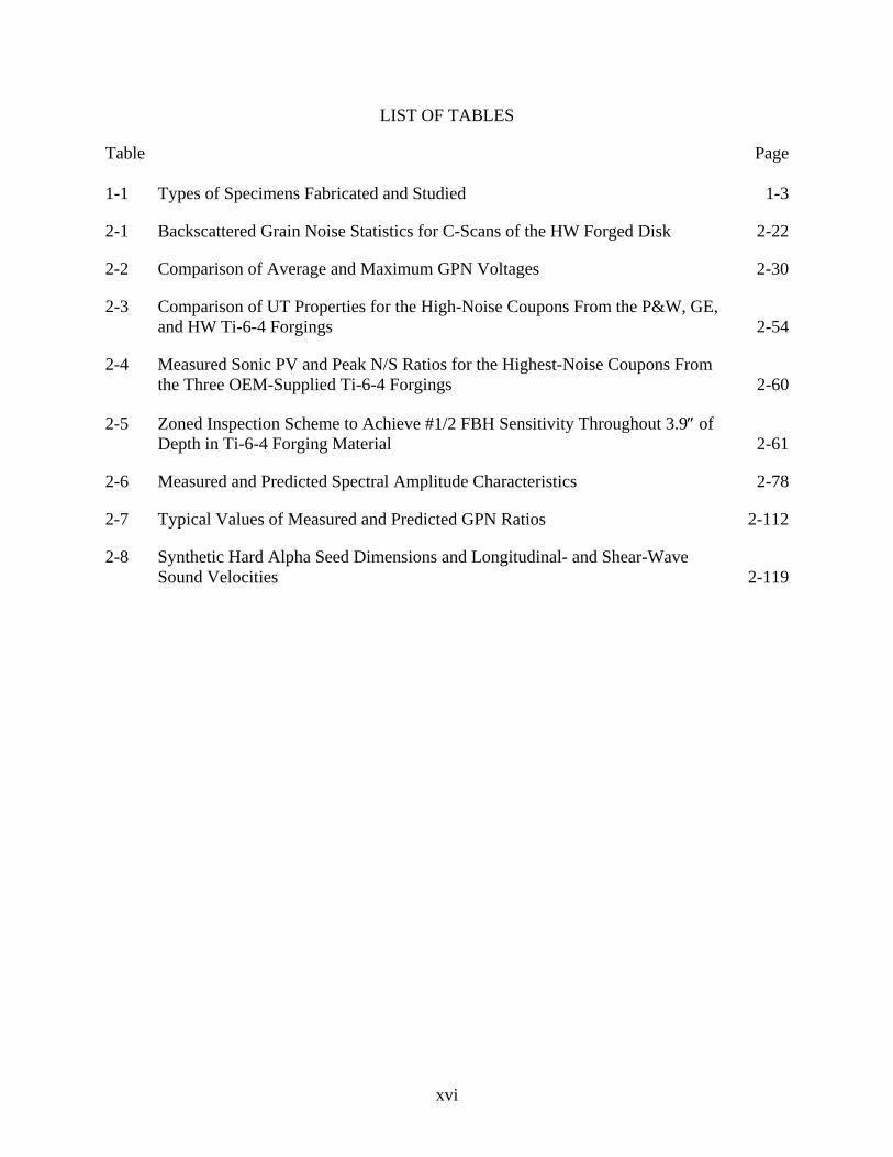
LIST OF TABLES

Table Page 1-1 Types of Specimens Fabricated and Studied 1-3

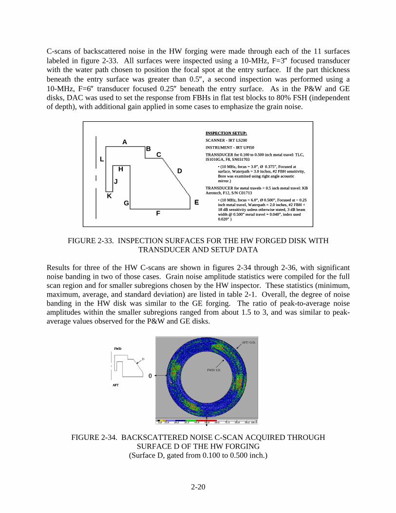
2-1 Backscattered Grain Noise Statistics for C-Scans of the HW Forged Disk 2-22

2-2 Comparison of Average and Maximum GPN Voltages 2-30

2-3 Comparison of UT Properties for the High-Noise Coupons From the P&W, GE, and HW Ti-6-4 Forgings 2-54

2-4 Measured Sonic PV and Peak N/S Ratios for the Highest-Noise Coupons From the Three OEM-Supplied Ti-6-4 Forgings 2-60

2-5 Zoned Inspection Scheme to Achieve #1/2 FBH Sensitivity Throughout 3.9″ of Depth in Ti-6-4 Forging Material 2-61

2-6 Measured and Predicted Spectral Amplitude Characteristics 2-78

2-7 Typical Values of Measured and Predicted GPN Ratios 2-112

2-8 Synthetic Hard Alpha Seed Dimensions and Longitudinal- and Shear-Wave Sound Velocities 2-119

xvii/xviii

LIST OF ACRONYMS

2D Two-dimensional DAC Distance-amplitude correction EDM Electron discharge machining ETC Engine Titanium Consortium FOM Figure of merit FQ Fused-quartz FBH Flat-bottom hole FSH Full-screen height GE General Electric Aircraft Engines GPN Gated-peak noise HIP Hot isostatic press HW Honeywell Engines, Systems & Services ID Inside diameter ISU Iowa State University N/S Noise-to-signal NAR Noise anisotropy ratio NDE Nondestructive evaluation Ni Nickel OD Outside diameter OEM Original equipment manufacturer P&W United Technologies Pratt & Whitney P/C Pitch/catch P/E Pulse/echo PoD Probability of detection PV Pulse volume RF Radio frequency rms Root mean square S/N Signal-to-noise SCL Spatial correlation length SID Synthetic inclusion disk Ti Titanium TT Through-transmission UT Ultrasonic

xix

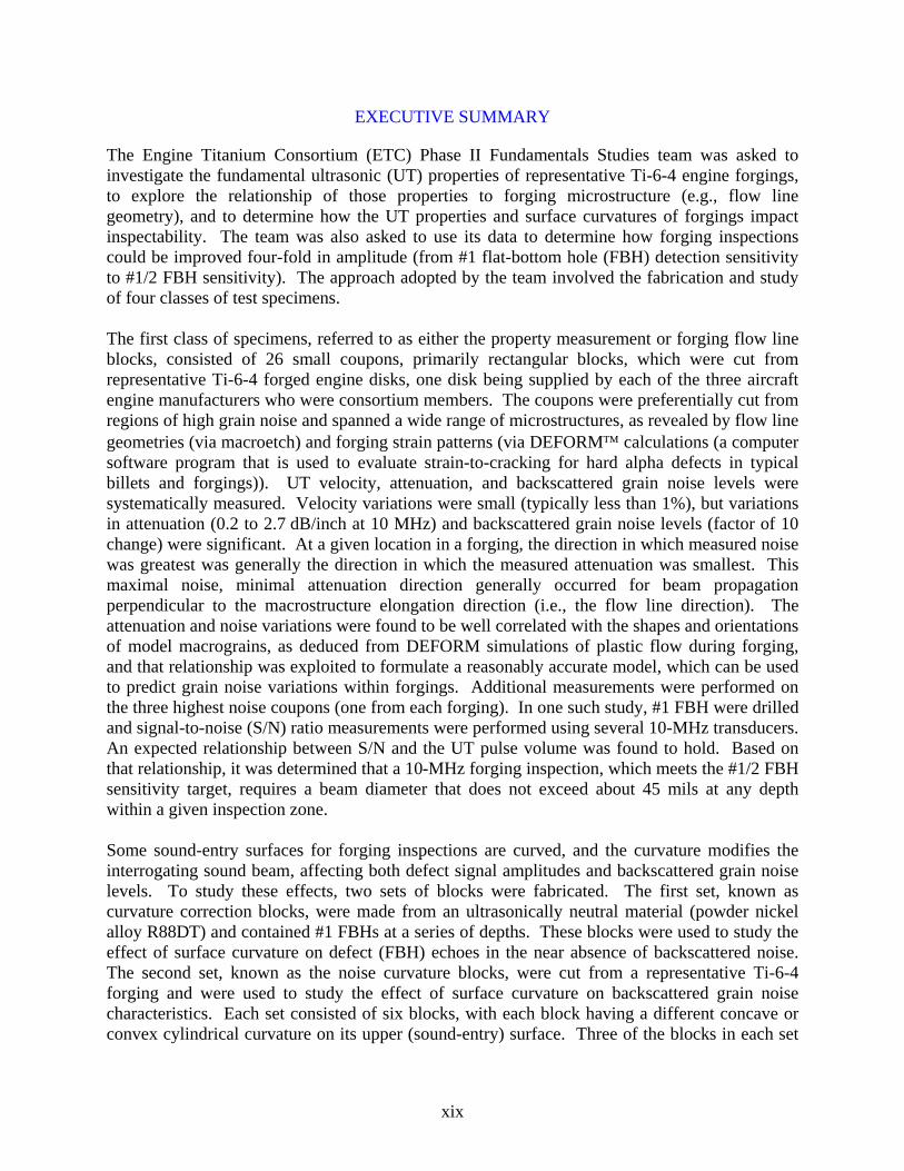
EXECUTIVE SUMMARY

The Engine Titanium Consortium (ETC) Phase II Fundamentals Studies team was asked to investigate the fundamental ultrasonic (UT) properties of representative Ti-6-4 engine forgings, to explore the relationship of those properties to forging microstructure (e.g., flow line geometry), and to determine how the UT properties and surface curvatures of forgings impact inspectability. The team was also asked to use its data to determine how forging inspections could be improved four-fold in amplitude (from #1 flat-bottom hole (FBH) detection sensitivity to #1/2 FBH sensitivity). The approach adopted by the team involved the fabrication and study of four classes of test specimens. The first class of specimens, referred to as either the property measurement or forging flow line blocks, consisted of 26 small coupons, primarily rectangular blocks, which were cut from representative Ti-6-4 forged engine disks, one disk being supplied by each of the three aircraft engine manufacturers who were consortium members. The coupons were preferentially cut from regions of high grain noise and spanned a wide range of microstructures, as revealed by flow line geometries (via macroetch) and forging strain patterns (via DEFORM™ calculations (a computer software program that is used to evaluate strain-to-cracking for hard alpha defects in typical billets and forgings)). UT velocity, attenuation, and backscattered grain noise levels were systematically measured. Velocity variations were small (typically less than 1%), but variations in attenuation (0.2 to 2.7 dB/inch at 10 MHz) and backscattered grain noise levels (factor of 10 change) were significant. At a given location in a forging, the direction in which measured noise was greatest was generally the direction in which the measured attenuation was smallest. This maximal noise, minimal attenuation direction generally occurred for beam propagation perpendicular to the macrostructure elongation direction (i.e., the flow line direction). The attenuation and noise variations were found to be well correlated with the shapes and orientations of model macrograins, as deduced from DEFORM simulations of plastic flow during forging, and that relationship was exploited to formulate a reasonably accurate model, which can be used to predict grain noise variations within forgings. Additional measurements were performed on the three highest noise coupons (one from each forging). In one such study, #1 FBH were drilled and signal-to-noise (S/N) ratio measurements were performed using several 10-MHz transducers. An expected relationship between S/N and the UT pulse volume was found to hold. Based on that relationship, it was determined that a 10-MHz forging inspection, which meets the #1/2 FBH sensitivity target, requires a beam diameter that does not exceed about 45 mils at any depth within a given inspection zone. Some sound-entry surfaces for forging inspections are curved, and the curvature modifies the interrogating sound beam, affecting both defect signal amplitudes and backscattered grain noise levels. To study these effects, two sets of blocks were fabricated. The first set, known as curvature correction blocks, were made from an ultrasonically neutral material (powder nickel alloy R88DT) and contained #1 FBHs at a series of depths. These blocks were used to study the effect of surface curvature on defect (FBH) echoes in the near absence of backscattered noise. The second set, known as the noise curvature blocks, were cut from a representative Ti-6-4 forging and were used to study the effect of surface curvature on backscattered grain noise characteristics. Each set consisted of six blocks, with each block having a different concave or convex cylindrical curvature on its upper (sound-entry) surface. Three of the blocks in each set

xx

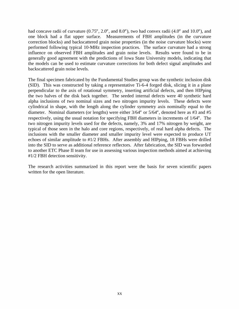
had concave radii of curvature (0.75″, 2.0″, and 8.0″), two had convex radii (4.0″ and 10.0″), and one block had a flat upper surface. Measurements of FBH amplitudes (in the curvature correction blocks) and backscattered grain noise properties (in the noise curvature blocks) were performed following typical 10-MHz inspection practices. The surface curvature had a strong influence on observed FBH amplitudes and grain noise levels. Results were found to be in generally good agreement with the predictions of Iowa State University models, indicating that the models can be used to estimate curvature corrections for both defect signal amplitudes and backscattered grain noise levels. The final specimen fabricated by the Fundamental Studies group was the synthetic inclusion disk (SID). This was constructed by taking a representative Ti-6-4 forged disk, slicing it in a plane perpendicular to the axis of rotational symmetry, inserting artificial defects, and then HIPping the two halves of the disk back together. The seeded internal defects were 40 synthetic hard alpha inclusions of two nominal sizes and two nitrogen impurity levels. These defects were cylindrical in shape, with the length along the cylinder symmetry axis nominally equal to the diameter. Nominal diameters (or lengths) were either 3/64″ or 5/64″, denoted here as #3 and #5 respectively, using the usual notation for specifying FBH diameters in increments of 1/64″. The two nitrogen impurity levels used for the defects, namely, 3% and 17% nitrogen by weight, are typical of those seen in the halo and core regions, respectively, of real hard alpha defects. The inclusions with the smaller diameter and smaller impurity level were expected to produce UT echoes of similar amplitude to #1/2 FBHs. After assembly and HIPping, 18 FBHs were drilled into the SID to serve as additional reference reflectors. After fabrication, the SID was forwarded to another ETC Phase II team for use in assessing various inspection methods aimed at achieving #1/2 FBH detection sensitivity. The research activities summarized in this report were the basis for seven scientific papers written for the open literature.

1-1

1. INTRODUCTION.

1.1 PURPOSE.

The complex microstructures of titanium (Ti) alloys typically used in aircraft engine forgings can significantly modify the signal strength from flaws and produce competing backscattered noise signals, which interfere with the detection of the flaws [1]. An understanding of ultrasonic (UT) wave propagation in these systems is needed to guide the development and application of inspection systems with the highest possible sensitivity, to develop algorithms to most accurately interpret the acquired data, and to provide a basis for evaluating their capability, e.g., in the determination of probability of detection (PoD). 1.2 BACKGROUND.

Phase I of the Engine Titanium Consortium (ETC) effort focused on developing a solid fundamental understanding of the nondestructive evaluation (NDE) characteristics of Ti jet engine alloys and the effect of microstructure on the detectability of defects such as hard alpha inclusions. Cylindrical Ti billets typically contain columnar macrograins that tend to align with the billet axis and have dimensions on the order of several millimeters. The macrograins themselves are comprised of much smaller micrograins, which have preferred orientations for their crystalline axes. Fundamental property measurements were performed in Phase I to investigate the effects of that micro- or macrostructure on UT beam propagation. In those measurements, rectangular coupons were cut from representative Ti-17 and Ti-6Al-4V billets, and sonic beams were propagated through the coupons in the radial, axial, and hoop directions. For each propagation direction, three UT quantities were measured: • Velocity, which determines the rate of beam focusing and diffraction;

• Attenuation, which describe the rate of decay of beam strength with penetration depth;

• Noise figure of merit (FOM), which describes the capacity of the microstructure for generating backscattered grain noise.

It was found that the direction of beam propagation relative to the billet macrostructure had a profound influence on the basic UT properties and, hence, on inspectability [2, 3, 4, and 5]. For example, grain noise levels were typically an order of magnitude smaller for propagation in the axial direction than in the radial or hoop direction. The columnar macrostructure was also found to distort the incident sonic beam, leading to significant excess signal attenuation and fluctuation effects. The severity of the distortion depended upon the beam propagation direction relative to the macrograin elongation direction, with the greatest distortions occurring when the beam traveled parallel to the elongation. In billet inspections, beam propagation is generally radially inward, approximately perpendicular to macrograin elongation; hence, beam distortion effects are minimized, but backscatter noise levels tend to be large. Flow lines in forged components are the counterparts of the elongated columnar macrograins in billets. It is, consequently, expected that the basic UT properties of forgings will depend strongly on the direction of sound propagation relative to the local flow line geometry.

1-2

Fundamental property measurements are thus needed to quantify the effects of forging microstructure on beam propagation and the corresponding effect on inspectability. In addition, the surface curvatures of forgings are more complex than those of billets, requiring measurements to determine the effects of curvature variations on flaw signal amplitudes, grain noise levels and signal-to-noise (S/N) ratios. The UT property data is critical to determining the sensitivity and PoD of forging inspections. The data will be used to test aspects of the inspection simulation models developed under other ETC subtasks. The combined experimental and theoretical understanding of UT wave propagation in titanium forgings will provide the basis for the design of forging inspection systems with improved sensitivity and for the assessment of their capabilities as needed for life management studies. 1.3 PROGRAM OBJECTIVES.

The objectives of this program were

• to gain the fundamental understanding of the UT properties of Ti forgings that is needed to provide a foundation for the development of reliable inspection methods that provide uniformly high sensitivity throughout the forging envelope.

• to acquire the data necessary to relate the detectability of defects in forgings to component properties (i.e., flow line characteristics and surface curvature) and defect properties (i.e., size, shape, composition, location, and orientation) thereby providing a foundation for the design of improved inspections and the evaluation of inspection capability.

1.4 RELATED ACTIVITIES AND DOCUMENTS.

The ETC was established in 1993 and includes Iowa State University (ISU), General Electric Aircraft Engines (GE), Honeywell Engines, Systems & Services (HW), and Pratt & Whitney (P&W) in a partnership to perform research that contributes to improvements in flight safety. The Phase I program, which was completed in 1998, led to improvements in production inspection of Ti billet [6], improved physics models for UTs [7 and 8], and a feasibility study for phased array for UT inspection of billets [9]. In-service inspection efforts led to a commercially available portable scanner [10] and eddy-current probes [11], as well as improved probe designs [12] and eddy-current probe design tools [13]. Considerable progress was also made in development of a new approach [14] to quantifying inspection performance as reported in an Federal Aviation Administration (FAA) report “A Methodology for the Assessment of the Capability of Inspection Systems for Detection of Subsurface Flaws in Engine Components” [15]. A sound understanding of the manner in which the UT properties of Ti alloys affect billet inspections was developed during ETC Phase I, as detailed in a lengthy FAA report, “Fundamental Studies: Inspection Properties for Engine Titanium Alloys” [16]. The work summarized in this report was performed under ETC Phase II Fundamental Property Measurements for Titanium Forgings. The research results and the fabricated specimens were made available to two companion ETC Phase II research teams: Inspection Development for Titanium Forgings used the UT property data and specimens in the design and testing of improved forging inspections, and PoD of Ultrasonic Inspections of Titanium Forgings was to

1-3

have used the UT property data in critiques of forging inspection schemes and probability of detection calculations, but that subtask was later suspended. 1.5 APPROACH.

The approach for this research effort consisted of the fabrication and study of the four classes of test specimens listed in table 1-1, which are briefly discussed below. Section 2 gives a more detailed discussion of the fabrication and uses of the test specimens.

TABLE 1-1. TYPES OF SPECIMENS FABRICATED AND STUDIED

Nomenclature Number of Specimens

(Alloy) Uses Property measurement blocks (or forging flow line coupons)

26 (Ti-6-4)

Measurement of basic UT properties of representative Ti-6-4 engine forgings. Study of the relationship between properties and forging flow lines (localized strain). Determination of sonic pulse volume requirements for improved forging inspections.

Curvature correction blocks

6 (nickel alloy R88DT)

To measure the effect of surface curvature on defect signal amplitudes and to test models that predict curvature correction factors for defect amplitudes.

Noise curvature blocks 6 (Ti-6-4)

To measure the effect of surface curvature on backscattered grain noise levels and to test models that predict curvature correction factors for grain noise.

Synthetic inclusion disk

1 (Ti-6-4)

Full-round disk with internal flaws (FBHs and synthetic hard alpha inclusions) for assessing various forging inspection methods.

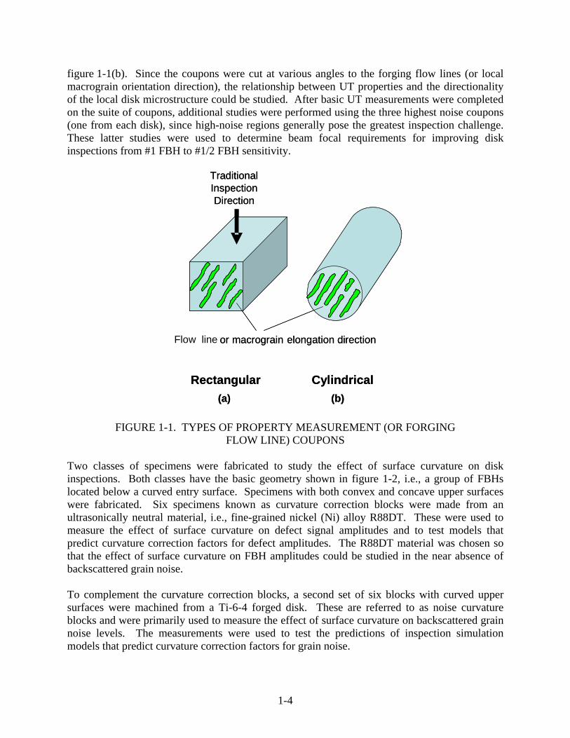
FBH = Flat-bottom hole The first class consisted of small coupons, primarily rectangular prisms, cut from representative Ti-6-4 forged engine disks. Each of the three aircraft engine manufacturers (P&W; GE; and HW) supplied one forging for this purpose, and a total of 26 coupons were cut from high-noise regions of these forgings. These coupons are referred to as either property measurement or forging flow line specimens, and they were used to measure fundamental UT properties (velocity, attenuation, and backscattered grain noise) for typical Ti-6-4 forgings. Most of the property-measurement coupons were rectangular blocks, as illustrated in figure 1-1(a), with one face perpendicular to the beam propagation direction for a standard, normal-incident, longitudinal-wave disk inspection. However, one coupon from each disk was a cylinder, which was used to study the angular dependence of backscattered grain noise, as illustrated in

1-4

figure 1-1(b). Since the coupons were cut at various angles to the forging flow lines (or local macrograin orientation direction), the relationship between UT properties and the directionality of the local disk microstructure could be studied. After basic UT measurements were completed on the suite of coupons, additional studies were performed using the three highest noise coupons (one from each disk), since high-noise regions generally pose the greatest inspection challenge. These latter studies were used to determine beam focal requirements for improving disk inspections from #1 FBH to #1/2 FBH sensitivity.

Rectangular Cylindrical

TraditionalInspectionDirection

or macrograin elongation direction

(a) (b)Rectangular Cylindrical

TraditionalInspectionDirection

Flow line or macrograin elongation direction

(a) (b)

FIGURE 1-1. TYPES OF PROPERTY MEASUREMENT (OR FORGING FLOW LINE) COUPONS

Two classes of specimens were fabricated to study the effect of surface curvature on disk inspections. Both classes have the basic geometry shown in figure 1-2, i.e., a group of FBHs located below a curved entry surface. Specimens with both convex and concave upper surfaces were fabricated. Six specimens known as curvature correction blocks were made from an ultrasonically neutral material, i.e., fine-grained nickel (Ni) alloy R88DT. These were used to measure the effect of surface curvature on defect signal amplitudes and to test models that predict curvature correction factors for defect amplitudes. The R88DT material was chosen so that the effect of surface curvature on FBH amplitudes could be studied in the near absence of backscattered grain noise. To complement the curvature correction blocks, a second set of six blocks with curved upper surfaces were machined from a Ti-6-4 forged disk. These are referred to as noise curvature blocks and were primarily used to measure the effect of surface curvature on backscattered grain noise levels. The measurements were used to test the predictions of inspection simulation models that predict curvature correction factors for grain noise.

1-5/1-6

FBH’s

Initial Shape

BA

CDE

- 2”- 4”flat4”

2”

Surface ProgressionBasic ShapeTypes of

Upper Surfaces

concave

convexFBH’s

Initial Shape

BA

CDE

- 2”- 4”flat4”

2”

Surface ProgressionBasic ShapeTypes of

Upper Surfaces

concave

convex

FIGURE 1-2. BASIC GEOMETRY OF SPECIMENS USED TO STUDY THE EFFECT OF SURFACE CURVATURE ON DISK INSPECTIONS

The final specimen fabricated under this effort was the Synthetic Inclusion Disk (SID). This was constructed by taking a representative Ti-6-4 forged disk, slicing it in a plane perpendicular to the axis of rotational symmetry, inserting artificial defects, and then hot isostatic pressing (HIP) the two halves of the disk back together. Internal defects were either FBH reflectors or spherical inclusions of synthetic hard alpha material. The SID was primarily fabricated for use in a companion Phase II study, Inspection Development for Titanium Forging, for assessing various forging inspection methods aimed at achieving #1/2 FBH sensitivity.

2-1

2. DISCUSSION OF RESULTS.

2.1 ULTRASONIC PROPERTIES OF FORGINGS AND THEIR IMPLICATIONS FOR FORGING INSPECTIONS.

A chief goal of this study was to document the manner in which UT properties vary within representative Ti-6-4 forgings and to use that data to help design improved forging inspections. In particular, the Inspection Development for Titanium Forging intended to use the UT data to design forging inspections that improve defect detection sensitivity four-fold, from the current #1 FBH level to a #1/2 FBH level. Since backscattered grain noise is primarily responsible for determining defect detection limits, an emphasis was placed on grain noise measurement and analysis. Each original equipment manufacturer (OEM) was asked to look through their inventory for potential forgings that could be used as sources for test samples. It was desired that the microstructures of the property measurement coupons be representative of the microstructures seen in typical forged engine components such as those studied in the Inspection Development for Titanium Forging. The OEMs supplied three typical forgings, and eight to ten coupons were cut from each. Coupon sites were chosen to provide a range of local microstructures based on backscattered noise, macroetch, and strain-map data. Measurements of UT longitudinal-wave velocity, attenuation, and backscattered noise were taken on the coupons and certain predictive models were developed to better understand the property data. The UT property data was also used to determine sonic beam-focusing requirements needed to achieve the # 1/2 FBH detection sensitivity target. This section describes that work. 2.2 COUPON SELECTION BASED ON GRAIN NOISE C-SCANS, MACROETCH, AND FORGING STRAIN INFORMATION.

Coupon selection from each forging was based on four factors: part dimension, flow line information, backscattered UT noise C-scans, and model simulations of forging strain. Coupons cut from a forging had to be large enough to permit straightforward measurement of UT properties. Once suitable-sized forgings were identified, UT pulse/echo (P/E) inspections were performed to map out backscattered grain noise patterns. Since the high-noise regions are presumably harder to inspect, they were given priority in coupon selection. The OEMs also provided flow line information (macroetch photographs) so coupons could be selected from both high and low flow line density regions. In addition, each OEM worked with its respective forging supplier to acquire forging strain maps, as predicted using DEFORM software [17]. Prior to actual fabrication of the property measurement coupons, some general design methodologies were developed. The coupons were principally designed for measurement of longitudinal-wave properties in the axial-radial plane, which are the interest of the current study. However, the coupon geometry will also allow measurements of shear-wave properties in the axial-hoop plane. These may be of interest to future researchers. Figure 2-1 depicts a portion of a generic sonic shape disk, with possible coupon sites indicated. Four rectangular coupons (A, C, D, and E) are indicated, with each having an entry face perpendicular to the beam

2-2

propagation direction for longitudinal-wave inspections (green arrows). The beam propagation direction for shear-wave inspections, if performed, is usually obtained by tilting the beam out of the plane of the page (e.g., into the Y Z plane for coupon E).

...

...

...

...

CL

A C E

D

portion of disk forging flow line

L - wave propagationdirection

...

...

...

...

CL

X (radial)

Y (axial)

Z (hoop)

A C E

D

portion of disk forging flow line

L - wave propagationdirection

FIGURE 2-1. EXAMPLES OF POSSIBLE PROPERTY MEASUREMENT COUPON SITES AND GEOMETRIES

As indicated in figure 2-1, it was desirable that coupons be cut from several locations in a forging with different local microstructures. Nearly all the coupons were chosen to be rectangular blocks with square cross sections in the radial-axial plane. This permitted comparative longitudinal-wave attenuation measurements to be performed for two propagation directions (e.g., axial and radial for coupon A) without complications arising from different thicknesses. In many cases, the two beam propagation directions were parallel and perpendicular, respectively, to the local flow lines. A small number of coupons with circular cross sections in the radial-axial plane were cut to better study the effect of flow line angle on backscattered noise. The rectangular coupons all had their longer dimension in the hoop direction. This design will permit future shear-wave attenuation measurements to be attempted using corner-trap echoes, as shown in figure 2-2 (left). If the use of corner-trap echoes proves to be problematic as is sometimes the case, a wedge could be cut (right) to facilitate shear-wave attenuation measurement. Both geometries shown in figure 2-2 have been used successfully in the past to measure attenuations in jet engine Ni alloys by comparison to a back-wall echo from a fused-quartz (FQ) reference block [18]. Inspections of Ti alloy forged disks typically reveal noise banding in the hoop (circumferential) direction, as illustrated in figure 2-3. In such cases, it was decided that property coupons would be cut from the high-noise regions of the disk, since defect detection is generally most difficult in such areas.

2-3

FIGURE 2-2. POSSIBLE SHEAR-WAVE ATTENUATION MEASUREMENT SETUPS

FIGURE 2-3. PREFERRED LOCATIONS IN FORGINGS FOR PROPERTY MEASUREMENT BLOCKS

These design considerations guided coupon site selection in the OEM-supplied forgings. The following sections discuss how the coupon sites were specifically chosen for each of the three OEM-supplied disks. For the GE, P&W, and HW disks, in turn, the key elements of the data used in coupon selection will be displayed. The displayed materials include (1) drawings showing the axial-radial cross sections of each disk; (2) photographs of macroetches of the cross sections of nominally identical disks revealing flow line structures; (3) outputs of DEFORM calculations showing metal deformation during the forging process; and (4) selected examples of

high noise quadrant

low no

ise qu

adran

thigh noise quadrant

low no

ise qu

adran

t

primary coupon sites

high noise quadrant

low no

ise qu

adran

thigh noise quadrant

low no

ise qu

adran

t

primary coupon sites

TiFQ BS1 CT1

45 shear wavein metal

o

same waterpath for both

Compare spectrum of corner-trap echo in Ti to that of back-wall echo in FQ

CT1

45 shear wave in metal

Alternative Geometry

Z (hoop)

Y (axial)

(typically)

o

2-4

C-scan images acquired by the OEMs during their respective inspections of the disks in question. The latter shows how backscattered noise levels vary with position within the forging. The specific coupon sites chosen for each forging will be indicated, and then the UT property measurements subsequently performed on the coupons themselves will be discussed. All the disk inspections performed to select coupon sites were focused-probe, normal incidence, P/E immersion inspections using longitudinal waves. It was noted that the three OEMs followed different protocols for inspecting disks, with each using different choices of transducers, inspection zones, and distance-amplitude correction (DAC) procedures. Thus, the noise C-scans supplied by different OEMs were not directly comparable to one another, although all could be used to infer the degree of noise banding and to identify the high-noise regions from which coupons were cut. After property measurement coupons were cut by the OEMs from their respective forgings, those coupons were shipped to ISU for UT measurements, which were all conducted following a uniform procedure. 2.2.1 Pratt & Whitney Disk.

The first disk considered was supplied by P&W. Figure 2-4 shows the general appearance of the disk (i.e., the sonic shape), and figure 2-5 shows the disk cross section with dimensional information. A macroetch of the cross section, revealing the flow line structure, is shown in figure 2-6. Figure 2-7 shows the results of a DEFORM simulation, which tracks plastic metal flow during the forging process. Small volume elements with circular cross sections in the radial-axial plane were specified in the billet blank, and these volume elements were then followed through the simulated forging process. As shown in figure 2-7(b), each circular element deformed into an ellipse, and areas of high forging strain have very elongated ellipses. FIGURE 2-4. COMPUTER-AIDED DRAWINGS OF THE P&W-SUPPLIED FORGED DISK

(Its inner and outer diameters are approximately 4.2 and 17.8 inches, respectively.)

2-5

FIGURE 2-5. CROSS SECTION OF THE SONIC SHAPE OF THE P&W-SUPPLIED FORGING, WITH INSPECTION SURFACES INDICATED

FIGURE 2-6. MACROETCH FOR THE P&W-SUPPLIED FORGING

Transducer: Nominal 3” focus, 3/8” diameter, 10 MHz Technisonic probe (N7135).Surfaces: Three inspection surfaces.Gating: Time interval between front and back wall echoes was divided into

4 time gates (different time gates for each inspection surface). Gain: Fixed waterpath with DAC. DAC set so that echoes from #1 FBHs in flat

calibration blocks were at 80% FSH. Then 15 dB of additional gain added.Increments: 0.02” scanning increments in the scan and index directions.

C.L.Surface 1

Surface 3Surface 2

2.1”

6.8”

3.3”

Surface Gate Depth_Range

1 1 0.20” - 0.56”1 2 0.56” - 0.93”1 3 0.93” - 1.29”1 4 1.29” - 1.62”2 1 0.20” - 0.87”2 2 0.87” - 1.54”2 3 1.54” - 2.21”2 4 2.21” - 2.88”3 1 0.18” - 0.91”3 2 0.91” - 1.64”3 3 1.64” - 2.37”3 4 2.37” - 3.08”

Surface Gate Depth_Range

1 1 0.20” - 0.56”1 2 0.56” - 0.93”1 3 0.93” - 1.29”1 4 1.29” - 1.62”2 1 0.20” - 0.87”2 2 0.87” - 1.54”2 3 1.54” - 2.21”2 4 2.21” - 2.88”3 1 0.18” - 0.91”3 2 0.91” - 1.64”3 3 1.64” - 2.37”3 4 2.37” - 3.08”

Transducer: Nominal 3” focus, 3/8” diameter, 10 MHz Technisonic probe (N7135).Surfaces: Three inspection surfaces.Gating: Time interval between front and back wall echoes was divided into

4 time gates (different time gates for each inspection surface). Gain: Fixed waterpath with DAC. DAC set so that echoes from #1 FBHs in flat

calibration blocks were at 80% FSH. Then 15 dB of additional gain added.Increments: 0.02” scanning increments in the scan and index directions.

C.L.Surface 1

Surface 3Surface 2

2.1”

6.8”

3.3”

C.L.Surface 1

Surface 3Surface 2

2.1”

6.8”

3.3”

Surface Gate Depth_Range

1 1 0.20” - 0.56”1 2 0.56” - 0.93”1 3 0.93” - 1.29”1 4 1.29” - 1.62”2 1 0.20” - 0.87”2 2 0.87” - 1.54”2 3 1.54” - 2.21”2 4 2.21” - 2.88”3 1 0.18” - 0.91”3 2 0.91” - 1.64”3 3 1.64” - 2.37”3 4 2.37” - 3.08”

Surface Gate Depth_Range

1 1 0.20” - 0.56”1 2 0.56” - 0.93”1 3 0.93” - 1.29”1 4 1.29” - 1.62”2 1 0.20” - 0.87”2 2 0.87” - 1.54”2 3 1.54” - 2.21”2 4 2.21” - 2.88”3 1 0.18” - 0.91”3 2 0.91” - 1.64”3 3 1.64” - 2.37”3 4 2.37” - 3.08”

Bore WebRim

Bore WebRim

2-6

(a) (b)

FIGURE 2-7. RESULTS OF A DEFORM CALCULATION FOR THE P&W FORGING

SHOWING HOW SMALL CIRCULAR ELEMENTS IN THE BILLET ARE DEFORMED BY THE FORGING PROCESS (a) BILLET SLICE BEFORE FORGING, WITH THE

CROSS-SECTIONAL AREA DIVIDED INTO CIRCULAR ELEMENTS AND (b) RESULTS OF THE FORGING PROCESS

2-7

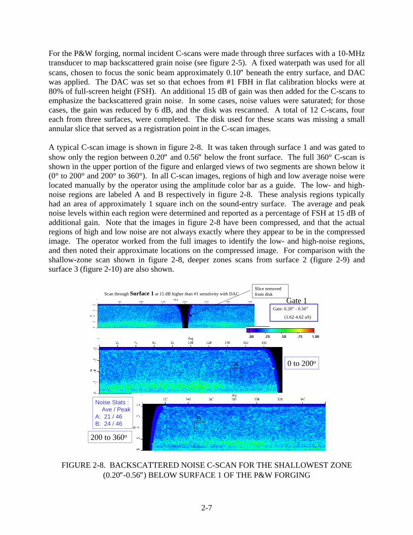
For the P&W forging, normal incident C-scans were made through three surfaces with a 10-MHz transducer to map backscattered grain noise (see figure 2-5). A fixed waterpath was used for all scans, chosen to focus the sonic beam approximately 0.10″ beneath the entry surface, and DAC was applied. The DAC was set so that echoes from #1 FBH in flat calibration blocks were at 80% of full-screen height (FSH). An additional 15 dB of gain was then added for the C-scans to emphasize the backscattered grain noise. In some cases, noise values were saturated; for those cases, the gain was reduced by 6 dB, and the disk was rescanned. A total of 12 C-scans, four each from three surfaces, were completed. The disk used for these scans was missing a small annular slice that served as a registration point in the C-scan images. A typical C-scan image is shown in figure 2-8. It was taken through surface 1 and was gated to show only the region between 0.20″ and 0.56″ below the front surface. The full 360° C-scan is shown in the upper portion of the figure and enlarged views of two segments are shown below it (0° to 200° and 200° to 360°). In all C-scan images, regions of high and low average noise were located manually by the operator using the amplitude color bar as a guide. The low- and high-noise regions are labeled A and B respectively in figure 2-8. These analysis regions typically had an area of approximately 1 square inch on the sound-entry surface. The average and peak noise levels within each region were determined and reported as a percentage of FSH at 15 dB of additional gain. Note that the images in figure 2-8 have been compressed, and that the actual regions of high and low noise are not always exactly where they appear to be in the compressed image. The operator worked from the full images to identify the low- and high-noise regions, and then noted their approximate locations on the compressed image. For comparison with the shallow-zone scan shown in figure 2-8, deeper zones scans from surface 2 (figure 2-9) and surface 3 (figure 2-10) are also shown.

FIGURE 2-8. BACKSCATTERED NOISE C-SCAN FOR THE SHALLOWEST ZONE

(0.20″-0.56″) BELOW SURFACE 1 OF THE P&W FORGING

Scan through Surface 1 at 15 dB higher than #1 sensitivity with DACSlice removedfrom disk

0 to 200o

200 to 360o

Gate: 0.20” - 0.56”

(1.62-4.62 uS)

Gate 1

A

B

Noise Stats : Ave / PeakA: 21 / 46B: 24 / 46

2-8

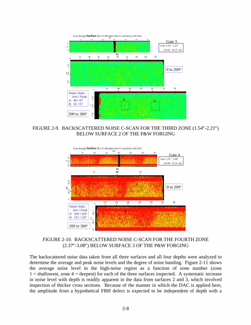
FIGURE 2-9. BACKSCATTERED NOISE C-SCAN FOR THE THIRD ZONE (1.54″-2.21″)

BELOW SURFACE 2 OF THE P&W FORGING

FIGURE 2-10. BACKSCATTERED NOISE C-SCAN FOR THE FOURTH ZONE

(2.37″-3.08″) BELOW SURFACE 3 OF THE P&W FORGING The backscattered noise data taken from all three surfaces and all four depths were analyzed to determine the average and peak noise levels and the degree of noise banding. Figure 2-11 shows the average noise level in the high-noise region as a function of zone number (zone 1 = shallowest, zone 4 = deepest) for each of the three surfaces inspected. A systematic increase in noise level with depth is readily apparent in the data from surfaces 2 and 3, which involved inspection of thicker cross sections. Because of the manner in which the DAC is applied here, the amplitude from a hypothetical FBH defect is expected to be independent of depth with a

Scan through Surface 2 at 15 dB higher than #1 sensitivity with DAC

0 to 200o

200 to 360o

Gate 3Gate: 1.54” - 2.21”

(12.62 - 18.12 uS)

Noise Stats : Ave / PeakA: 48 / 87B: 52 / 97

B A

Scan through Surface 3 at 15 dB higher than #1 sensitivity with DAC

0 to 200o

Gate 4Gate: 2.37” - 3.08”

(19.44 - 25.24 uS)

A

BNoise Stats : Ave / PeakA: 100 / 169B: 121 / 197

200 to 360o

2-9

constant amplitude of 450% FSH (i.e., 15 dB above 80%). Thus, the noise levels measured may be thought of as being noise-to-signal (N/S) ratios. Studies conducted during ETC Phase I have shown that for typical inspection scenarios, N/S tends to grow like the square root of the sonic pulse volume (PV) when the noise is microstructural in origin. Thus, N/S tends to be smallest near the focal zone of a sound beam, and to increase as one moves away from the focal zone, other factors (e.g., microstructure) being constant [16].

FIGURE 2-11. AVERAGE NOISE LEVELS IN THE HIGH-NOISE

REGIONS OF THE P&W FORGING The dependence of noise level (or N/S) on inspection depth is more explicitly shown in figure 2-12. There the average and peak noise levels in the high-noise regions have been plotted as a function of the maximum depth within the inspection zone. The 12 values in figure 2-11 have, thus, been replotted to produce the lower (blue) curve in figure 2-12, and the peak noise values are similarly plotted in the upper (red) curve. The general dependence on depth shown in figure 2-12 is believed to be principally due to the spreading of the sonic beam that was focused just below the entry surface for these measurements.

FIGURE 2-12. AVERAGE AND PEAK NOISE LEVELS FOR HIGH-NOISE

REGIONS OF THE P&W FORGING

0

20

40

60

80

100

120

140

160

S1 S2 S3

Surface

Noi

se L

evel

(%

FSH

)Zone 1 Zone 2Zone 3 Zone 4

0

50

100

150

200

250

0.0 1.0 2.0 3.0 4.0

Max Depth in Zone (inches)

Noi

se L

evel

(%

FSH

) Ave-HighPeak-High

2-10

The degree of noise banding in the circumferential direction was evaluated by plotting the average high-noise amplitude divided by the average low-noise amplitude for each zone of all three surfaces. The result, shown in figure 2-13, indicates that very little noise banding was observed in the P&W forging, with the high- to low-noise ratio ranging only from 1.0 to 1.2.

FIGURE 2-13. RATIO OF AVERAGE NOISE LEVELS IN HIGH- AND LOW-NOISE

REGIONS OF THE P&W FORGING The peak noise level observed within a region of a forging C-scan will always exceed the average noise level within that same region. The peak-to-average ratio is often of interest from a PoD standpoint, and this ratio is plotted versus zone depth in figure 2-14. For the P&W forging, the peak and average noise levels in a given 1-square-inch region typically differ by about a factor of 2.

FIGURE 2-14. RATIO OF PEAK TO AVERAGE NOISE AS A FUNCTION OF

DEPTH IN THE P&W FORGING

0.6

0.7

0.8

0.9

1.0

1.1

1.2

1.3

S1 S2 S3

Surface

Ave

-Hig

h / A

ve-L

ow

Zone 1 Zone 2Zone 3 Zone 4

0.0

0.5

1.0

1.5

2.0

2.5

0.0 1.0 2.0 3.0 4.0

Max Depth in Zone (inches)

Peak

/ A

vera

ge

Low noise regions

High noise regions

2-11

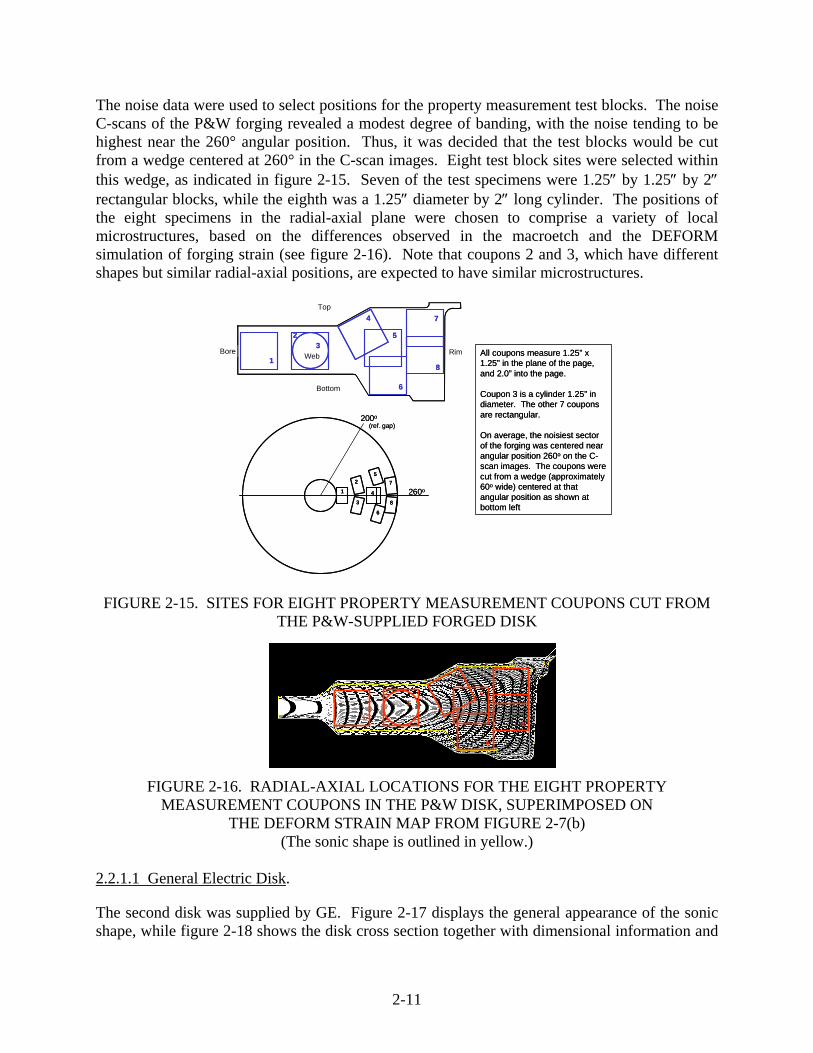
The noise data were used to select positions for the property measurement test blocks. The noise C-scans of the P&W forging revealed a modest degree of banding, with the noise tending to be highest near the 260° angular position. Thus, it was decided that the test blocks would be cut from a wedge centered at 260° in the C-scan images. Eight test block sites were selected within this wedge, as indicated in figure 2-15. Seven of the test specimens were 1.25″ by 1.25″ by 2″ rectangular blocks, while the eighth was a 1.25″ diameter by 2″ long cylinder. The positions of the eight specimens in the radial-axial plane were chosen to comprise a variety of local microstructures, based on the differences observed in the macroetch and the DEFORM simulation of forging strain (see figure 2-16). Note that coupons 2 and 3, which have different shapes but similar radial-axial positions, are expected to have similar microstructures. FIGURE 2-15. SITES FOR EIGHT PROPERTY MEASUREMENT COUPONS CUT FROM

THE P&W-SUPPLIED FORGED DISK

FIGURE 2-16. RADIAL-AXIAL LOCATIONS FOR THE EIGHT PROPERTY MEASUREMENT COUPONS IN THE P&W DISK, SUPERIMPOSED ON

THE DEFORM STRAIN MAP FROM FIGURE 2-7(b) (The sonic shape is outlined in yellow.)

2.2.1.1 General Electric Disk.

The second disk was supplied by GE. Figure 2-17 displays the general appearance of the sonic shape, while figure 2-18 shows the disk cross section together with dimensional information and

All coupons measure 1.25” x 1.25” in the plane of the page, and 2.0” into the page.

Coupon 3 is a cylinder 1.25” in diameter. The other 7 coupons are rectangular.

On average, the noisiest sector of the forging was centered near angular position 260o on the C-scan images. The coupons were cut from a wedge (approximately 60o wide) centered at that angular position as shown at bottom left

Bore Web Rim1

23

4

5

6

7

8

Top

Bottom

260o1

2

34

5

6

7

8

200o

(ref. gap)

All coupons measure 1.25” x 1.25” in the plane of the page, and 2.0” into the page.

Coupon 3 is a cylinder 1.25” in diameter. The other 7 coupons are rectangular.

On average, the noisiest sector of the forging was centered near angular position 260o on the C-scan images. The coupons were cut from a wedge (approximately 60o wide) centered at that angular position as shown at bottom left

Bore Web Rim1

23

4

5

6

7

8

Top

Bottom

260o1

2

34

5

6

7

8

200o

(ref. gap)

1

23

4

5

6

7

81

23

4

5

6

7

8

2-12

some UT inspection details. A macroetch of the cross section, revealing the flow line structure, is shown in figure 2-19. Figure 2-20 shows the results of a DEFORM simulation for plastic metal flow during the forging process. Again, small volume elements with circular cross sections in the radial-axial plane were specified in the billet blank, and these volume elements were followed through the forging process. Each OEM worked with a different forging supplier to perform DEFORM simulations and to document the outputs. Different suppliers were able to perform such calculations and display the results with differing degrees of sophistication. For example, the DEFORM results for the P&W disk shown in figure 2-7 have a different format than that shown in figure 2-20 for the GE disk. An alternative method for displaying DEFORM results is shown in figure 2-21, where the calculated forging strain magnitudes in the radial-axial plane are displayed as a function of position.

FIGURE 2-17. GENERAL APPEARANCE OF THE GE-SUPPLIED FORGED DISK BEFORE THE BORE HOLE WAS CUT

(Sonic shape is approximately 22″ in diameter with a 9″ diameter central hole.)

FIGURE 2-18. CROSS SECTION OF THE SONIC SHAPE OF THE GE-SUPPLIED FORGING

There were two inspection zones for all surfaces exceptUK (Zone 1 only) and UG (Zones 1-4).

The zoning scheme was:

Zone 1, calibrated 0.06" to 0.5", gated 0.06" to 0.6".Zone 2, calibrated 0.5" to 1.0", gated 0.4" to 1.1".Zone 3, calibrated 1.0" to 1.5", gated 0.9" to 1.6".Zone 4, calibrated 1.5" to 2.0", gated 1.4" to 2.1".

Two probes were used:I3 (10 MHz, 0.375” dia. F= 3”) andF8 (10 MHz, 1” dia. F= 8”)

Zone 1 used I3 Zone 2 used F8 (except UJ,UR,UZ)Zones 3 & 4 used F8.

US

CenterLine

UG(3 3/4”)

UR

UP

UO(1”)

UZ(1 15/32”)

UM(1 1/16”)

ULUK

UJ

UH (1 15/16”)6 9/16”

4.5”

US (11/16”)

7/16”

Lengths of selectedsurfaces are indicated.

There were two inspection zones for all surfaces exceptUK (Zone 1 only) and UG (Zones 1-4).

The zoning scheme was:

Zone 1, calibrated 0.06" to 0.5", gated 0.06" to 0.6".Zone 2, calibrated 0.5" to 1.0", gated 0.4" to 1.1".Zone 3, calibrated 1.0" to 1.5", gated 0.9" to 1.6".Zone 4, calibrated 1.5" to 2.0", gated 1.4" to 2.1".

Two probes were used:I3 (10 MHz, 0.375” dia. F= 3”) andF8 (10 MHz, 1” dia. F= 8”)

Zone 1 used I3 Zone 2 used F8 (except UJ,UR,UZ)Zones 3 & 4 used F8.

US

CenterLine

UG(3 3/4”)

UR

UP

UO(1”)

UZ(1 15/32”)

UM(1 1/16”)

ULUK

UJ

UH (1 15/16”)6 9/16”

4.5”

US (11/16”)

7/16”

Lengths of selectedsurfaces are indicated.

US

CenterLine

UG(3 3/4”)

UR

UP

UO(1”)

UZ(1 15/32”)

UM(1 1/16”)

ULUK

UJ

UH (1 15/16”)6 9/16”

4.5”

US (11/16”)

7/16”

Lengths of selectedsurfaces are indicated.

2-13

FIGURE 2-19. MACROETCH FOR THE GE-SUPPLIED FORGING (The approximate boundary of the sonic shape is indicated.)

FIGURE 2-20. RESULTS OF A DEFORM CALCULATION FOR THE GE FORGING, SHOWING HOW SMALL CIRCULAR ELEMENTS IN THE BILLET ARE

DEFORMED BY THE FORGING PROCESS

FIGURE 2-21. RELATIVE FORGING STRAIN LEVELS AS CALCULATED BY DEFORM FOR THE GE FORGING IN ARBITRARY UNITS

(The as-forged cross section is shown with the white line indicating the boundary of the sonic shape.)

Bore

Web

Rim

Bore

Web

Rim

Billet Blank

GE Forging

Billet Blank

GE Forging

0 1.2 2.4 3.6 4.8 6.0 7.2 8.4 9.6 10.8 12.0 Radius (inches)

-1.2

0.0

1.2

2.4

3.64.5

4.0

3.5

3.0

2.5

2.0

1.5

1.0

0.5

Low Strain(0.238)

High Strain(5.411)

Hei

ght

(inch

es)

GE Ti 6-4 Forging

0 1.2 2.4 3.6 4.8 6.0 7.2 8.4 9.6 10.8 12.0 Radius (inches)

-1.2

0.0

1.2

2.4

3.64.5

4.0

3.5

3.0

2.5

2.0

1.5

1.0

0.5

Low Strain(0.238)

High Strain(5.411)

Hei

ght

(inch

es)

0 1.2 2.4 3.6 4.8 6.0 7.2 8.4 9.6 10.8 12.0 Radius (inches)

-1.2

0.0

1.2

2.4

3.64.5

4.0

3.5

3.0

2.5

2.0

1.5

1.0

0.5

Low Strain(0.238)

High Strain(5.411)

0 1.2 2.4 3.6 4.8 6.0 7.2 8.4 9.6 10.8 12.0 Radius (inches)

-1.2

0.0

1.2

2.4

3.64.5

4.0

3.5

3.0

2.5

2.0

1.5

1.0

0.5

Low Strain(0.238)

High Strain(5.411)

Hei

ght

(inch

es)

GE Ti 6-4 Forging

2-14

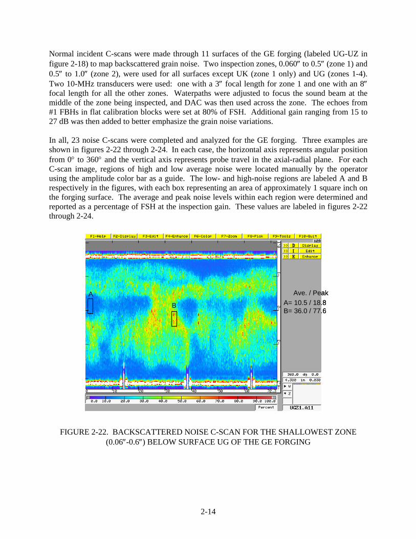
Normal incident C-scans were made through 11 surfaces of the GE forging (labeled UG-UZ in figure 2-18) to map backscattered grain noise. Two inspection zones, 0.060″ to 0.5″ (zone 1) and 0.5″ to 1.0″ (zone 2), were used for all surfaces except UK (zone 1 only) and UG (zones 1-4). Two 10-MHz transducers were used: one with a 3″ focal length for zone 1 and one with an 8″ focal length for all the other zones. Waterpaths were adjusted to focus the sound beam at the middle of the zone being inspected, and DAC was then used across the zone. The echoes from #1 FBHs in flat calibration blocks were set at 80% of FSH. Additional gain ranging from 15 to 27 dB was then added to better emphasize the grain noise variations. In all, 23 noise C-scans were completed and analyzed for the GE forging. Three examples are shown in figures 2-22 through 2-24. In each case, the horizontal axis represents angular position from 0° to 360° and the vertical axis represents probe travel in the axial-radial plane. For each C-scan image, regions of high and low average noise were located manually by the operator using the amplitude color bar as a guide. The low- and high-noise regions are labeled A and B respectively in the figures, with each box representing an area of approximately 1 square inch on the forging surface. The average and peak noise levels within each region were determined and reported as a percentage of FSH at the inspection gain. These values are labeled in figures 2-22 through 2-24.

FIGURE 2-22. BACKSCATTERED NOISE C-SCAN FOR THE SHALLOWEST ZONE (0.06″-0.6″) BELOW SURFACE UG OF THE GE FORGING

A

B A= 10.5 / 18.8B= 36.0 / 77.6

Ave. / PeakA

B

A

B A= 10.5 / 18.8B= 36.0 / 77.6

Ave. / Peak

2-15

FIGURE 2-23. BACKSCATTERED NOISE C-SCAN FOR THE SECOND ZONE (0.5″-1.0″)

BELOW SURFACE UO OF THE GE FORGING

FIGURE 2-24. SITES FOR PROPERTY MEASUREMENT COUPONS CUT FROM THE

GE-SUPPLIED FORGED DISK

UOZ2F8.pcx 25May00 0.5” x 2” analysis regions

A

B

A= 10.9 / 23.5B= 40.7 / 87.8

Ave. / Peak

UGZ4F8.pcx 25May00 0.25” x 4” analysis regions

A

B

A= 7.0 / 12.5B= 42.3 / 85.4

Ave. / Peak

2-16

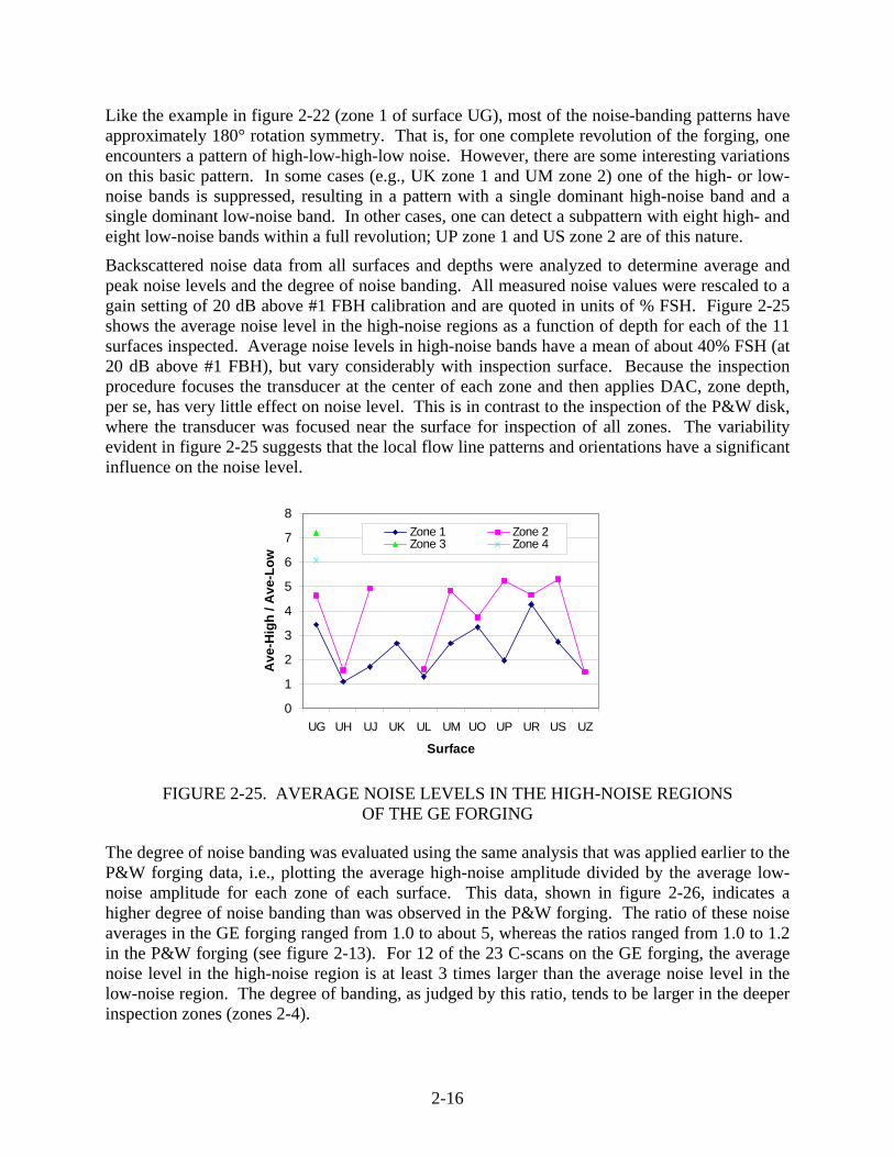
Like the example in figure 2-22 (zone 1 of surface UG), most of the noise-banding patterns have approximately 180° rotation symmetry. That is, for one complete revolution of the forging, one encounters a pattern of high-low-high-low noise. However, there are some interesting variations on this basic pattern. In some cases (e.g., UK zone 1 and UM zone 2) one of the high- or low-noise bands is suppressed, resulting in a pattern with a single dominant high-noise band and a single dominant low-noise band. In other cases, one can detect a subpattern with eight high- and eight low-noise bands within a full revolution; UP zone 1 and US zone 2 are of this nature.

Backscattered noise data from all surfaces and depths were analyzed to determine average and peak noise levels and the degree of noise banding. All measured noise values were rescaled to a gain setting of 20 dB above #1 FBH calibration and are quoted in units of % FSH. Figure 2-25 shows the average noise level in the high-noise regions as a function of depth for each of the 11 surfaces inspected. Average noise levels in high-noise bands have a mean of about 40% FSH (at 20 dB above #1 FBH), but vary considerably with inspection surface. Because the inspection procedure focuses the transducer at the center of each zone and then applies DAC, zone depth, per se, has very little effect on noise level. This is in contrast to the inspection of the P&W disk, where the transducer was focused near the surface for inspection of all zones. The variability evident in figure 2-25 suggests that the local flow line patterns and orientations have a significant influence on the noise level.

FIGURE 2-25. AVERAGE NOISE LEVELS IN THE HIGH-NOISE REGIONS

OF THE GE FORGING The degree of noise banding was evaluated using the same analysis that was applied earlier to the P&W forging data, i.e., plotting the average high-noise amplitude divided by the average low-noise amplitude for each zone of each surface. This data, shown in figure 2-26, indicates a higher degree of noise banding than was observed in the P&W forging. The ratio of these noise averages in the GE forging ranged from 1.0 to about 5, whereas the ratios ranged from 1.0 to 1.2 in the P&W forging (see figure 2-13). For 12 of the 23 C-scans on the GE forging, the average noise level in the high-noise region is at least 3 times larger than the average noise level in the low-noise region. The degree of banding, as judged by this ratio, tends to be larger in the deeper inspection zones (zones 2-4).

0

1

2

3

4

5

6

7

8

UG UH UJ UK UL UM UO UP UR US UZ

Surface

Ave

-Hig

h / A

ve-L

ow

Zone 1 Zone 2Zone 3 Zone 4

2-17

FIGURE 2-26. RATIO OF AVERAGE NOISE LEVELS IN HIGH- AND

LOW-NOISE REGIONS OF THE GE FORGING As was done earlier for the P&W forging, the ratio of peak-to-average noise was computed for each 1″ square analysis region, as shown in figure 2-27 for the GE disk. In any given analysis region, the ratio of the peak noise pixel value to the average noise value was typically about 2. This was true for both the low- and high-noise regions. These results are very similar to those from the P&W forging (see figure 2-14), where the ratio varied from about 1.5 to 2.2. The one major exception was surface UL, zone 2, which has a region of elevated noise in a narrow angular range.

Figure 2-27. RATIO OF PEAK-TO-AVERAGE NOISE IN THE GE FORGING

As with the P&W forging, the GE noise data was used to select locations for the property measurement test blocks. Eight coupon sites were selected; their approximate locations are shown in figure 2-28. The data indicated that one angular section of the bore and web regions of the disk tended to have a higher noise level. All eight coupons were cut from this octant, as shown in figure 2-28. Seven of the coupons were rectangular prisms, while the eighth

0

10

20

30

40

50

60

70

80

90

UG UH UJ UK UL UM UO UP UR US UZ

Surface

Noi

se L

evel

(%

FSH

)

Zone 1 Zone 2Zone 3 Zone 4

0

1

2

3

4

5

UG UH UJ UK UL UM UO UP UR US UZ

Surface

Peak

/ A

vera

ge

Zone 1; Low Zone 2; LowZone 1; High Zone 2; High

2-18

(coupon 2) was a cylinder that was expected to have a similar microstructure to rectangular coupon #1. As for the P&W disk, the test coupon locations in the radial-axial plane were chosen using the macroetch and DEFORM results to provide a variety of flow line geometries relative to the beam propagation direction.

FIGURE 2-28. SITES FOR PROPERTY MEASUREMENT COUPONS CUT FROM THE

GE-SUPPLIED FORGED DISK 2.2.1.2 Honeywell Disk.

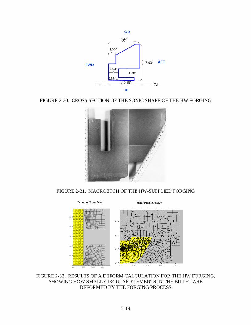
The last of the three Ti-6-4 forgings used as sources for property measurement coupons was supplied by HW. Figure 2-29 displays the general appearance of the sonic shape, while figure 2-30 shows the disk cross section, with dimensional information. A macroetch of the cross section, revealing the flow line structure, is shown in figure 2-31. Figure 2-32 shows the results of a DEFORM simulation of the forging process in the same spirit as the P&W and GE forgings.

FIGURE 2-29. GENERAL APPEARANCE OF THE HW-SUPPLIED FORGED DISK (The ruler is about 6.5″ long.)

US

UG

UR

UPUO

UZ

UMUL

UK

UJ

UH

US

12

4

58

3

6

7

Coupons 1,4,5,6,7 are rectangles approx. 1.25” x 1.25” x 2.0”.Coupon 3 is a rectangle approx. 0.5” x 0.5” x 2.0”.Coupon 8 is a rectangle approx. 1.0” x 1.0” x 2.0”.Coupon 2 is a cylinder approx. 1.25” diameter by 2.0” long.

Note that each rectangular coupon has two sides the same length.

Sites for 8 coupons cut from the GE-supplied forging.

Note that sites 1 and 2 are expected to have similar microstructures. All coupons are 2” long in the “hoop” direction.

Highest noise octantof disk, as judged from UO, UM, UK C-scans

3

6

7

12 4, 5

8

US

UG

UR

UPUO

UZ

UMUL

UK

UJ

UH

US

12

4

58

3

6

7

US

UG

UR

UPUO

UZ

UMUL

UK

UJ

UH

US

12

4

58

3

6

7

Coupons 1,4,5,6,7 are rectangles approx. 1.25” x 1.25” x 2.0”.Coupon 3 is a rectangle approx. 0.5” x 0.5” x 2.0”.Coupon 8 is a rectangle approx. 1.0” x 1.0” x 2.0”.Coupon 2 is a cylinder approx. 1.25” diameter by 2.0” long.

Note that each rectangular coupon has two sides the same length.

Sites for 8 coupons cut from the GE-supplied forging.

Note that sites 1 and 2 are expected to have similar microstructures. All coupons are 2” long in the “hoop” direction.

Highest noise octantof disk, as judged from UO, UM, UK C-scans

3

6

7

12 4, 5

8 Highest noise octantof disk, as judged from UO, UM, UK C-scans

Highest noise octantof disk, as judged from UO, UM, UK C-scans

3

6

7

12 4, 5

8

2-19

FIGURE 2-30. CROSS SECTION OF THE SONIC SHAPE OF THE HW FORGING

FIGURE 2-31. MACROETCH OF THE HW-SUPPLIED FORGING

FIGURE 2-32. RESULTS OF A DEFORM CALCULATION FOR THE HW FORGING, SHOWING HOW SMALL CIRCULAR ELEMENTS IN THE BILLET ARE

DEFORMED BY THE FORGING PROCESS

ID

AFTFWD

OD

7.63″

1.88″

0.65″0.85″

6.43″

CL

1.55″

1.93″

Billet in Upset Dies After Finisher stageBillet in Upset Dies After Finisher stage

2-20

C-scans of backscattered noise in the HW forging were made through each of the 11 surfaces labeled in figure 2-33. All surfaces were inspected using a 10-MHz, F=3″ focused transducer with the water path chosen to position the focal spot at the entry surface. If the part thickness beneath the entry surface was greater than 0.5″, a second inspection was performed using a 10-MHz, F=6″ transducer focused 0.25″ beneath the entry surface. As in the P&W and GE disks, DAC was used to set the response from FBHs in flat test blocks to 80% FSH (independent of depth), with additional gain applied in some cases to emphasize the grain noise.

FIGURE 2-33. INSPECTION SURFACES FOR THE HW FORGED DISK WITH TRANSDUCER AND SETUP DATA

Results for three of the HW C-scans are shown in figures 2-34 through 2-36, with significant noise banding in two of those cases. Grain noise amplitude statistics were compiled for the full scan region and for smaller subregions chosen by the HW inspector. These statistics (minimum, maximum, average, and standard deviation) are listed in table 2-1. Overall, the degree of noise banding in the HW disk was similar to the GE forging. The ratio of peak-to-average noise amplitudes within the smaller subregions ranged from about 1.5 to 3, and was similar to peak-average values observed for the P&W and GE disks.

FIGURE 2-34. BACKSCATTERED NOISE C-SCAN ACQUIRED THROUGH SURFACE D OF THE HW FORGING

(Surface D, gated from 0.100 to 0.500 inch.)

AB

C

D

EF

H

J

GK

L

INSPECTION SETUP:

SCANNER - IRT LS200

INSTRUMENT - IRT UPI50

TRANSDUCER for 0.100 to 0.500 inch metal travel: TLC, IS1010GA, F8, SN031703

• (10 MHz, focus = 3.0”, Ø 0.375”, Focused at surface, Waterpath = 3.0 inches, #2 FBH sensitivity, Bore was examined using right angle acoustic mirror.)

TRANSDUCER for metal travels > 0.5 inch metal travel: KB Aerotech, F12, S/N C01713

• (10 MHz, focus = 6.0”, Ø 0.500”, Focused at ~ 0.25 inch metal travel, Waterpath = 2.0 inches, #2 FBH + 18 dB sensitivity unless otherwise stated, 3 dB beam width @ 0.500” metal travel = 0.040”, index used 0.020” )

AB

C

D

EF

H

J

GK

L

INSPECTION SETUP:

SCANNER - IRT LS200

INSTRUMENT - IRT UPI50

TRANSDUCER for 0.100 to 0.500 inch metal travel: TLC, IS1010GA, F8, SN031703

• (10 MHz, focus = 3.0”, Ø 0.375”, Focused at surface, Waterpath = 3.0 inches, #2 FBH sensitivity, Bore was examined using right angle acoustic mirror.)

TRANSDUCER for metal travels > 0.5 inch metal travel: KB Aerotech, F12, S/N C01713

• (10 MHz, focus = 6.0”, Ø 0.500”, Focused at ~ 0.25 inch metal travel, Waterpath = 2.0 inches, #2 FBH + 18 dB sensitivity unless otherwise stated, 3 dB beam width @ 0.500” metal travel = 0.040”, index used 0.020” )

0FWD/ I.D.

AFT/ O.D.

AFT

FWD

D

0FWD/ I.D.

AFT/ O.D.

AFT

FWD

D

AFT

FWD

D

2-21

FIGURE 2-35. BACKSCATTERED NOISE C-SCAN ACQUIRED THROUGH SURFACE F OF THE HW FORGING

(Surface F, gated from a 0.100- to 0.500-inch C-scan shown aft looking forward.)

FIGURE 2-36. BACKSCATTERED NOISE C-SCAN ACQUIRED THROUGH SURFACE A OF THE HW FORGING

(Surface A, gated from 0.50 to 1.00 inch.)

0° I.D.

O.D.

F

FWD

AFT

0° I.D.

O.D.

F

FWD

AFTF

FWD

AFT

0°I.D.

O.D.

FWD A

AFT

0°I.D.

O.D.

FWD A

AFT

FWD A

AFT

2-22

TABLE 2-1. BACKSCATTERED GRAIN NOISE STATISTICS FOR C-SCANS OF THE HW FORGED DISK

Surface Gated Range

in Inches

Min. Amp.

% FSH

Ave. Amp. %FSH

Max. Amp. %FSH

Std. Dev. Notes

A 0.100 to 0.500 7.8 21.1 70.5 1.9 Entire scan area (70.5 max. on 1 to 3 individual pixels)

A 0.100 to 0.500 7.8 21.1 34.5 1.9 Average clean area A 0.100 to 0.500 7.8 16.4 25.1 3.5 Low-amplitude area (1-area) B 0.100 to 0.500 16.4 26.6 46.2 1.9 Entire scan area B 0.100 to 0.500 16.4 24.3 30.5 1.1 Average clean area B 0.100 to 0.500 21.9 28.2 37.6 1.5 High-amplitude area (2-areas) C 0.100 to 0.500 10.9 21.5 32.1 1.9 Entire scan area C 0.100 to 0.500 18.8 25.4 32.1 1.9 Single line, high-amplitude area

(1-area) D 0.100 to 0.500 9.4 26.2 98.4+ 7.0 Entire scan area D 0.100 to 0.500 14.1 23.9 58.8 3.9 Average clean area D 0.100 to 0.500 14.5 31.3 93.0 8.8 Average high-amplitude area

(4-areas) E 0.100 to 0.500 7.8 22.3 72.9 5.4 Entire scan area E 0.100 to 0.500 9.4 20.0 48.6 3.5 Average clean area E 0.100 to 0.500 15.2 26.5 61.1 5.4 Average high-amplitude area

(5-areas) F 0.100 to 0.500 18.0 33.3 97.2 6.6 Entire scan area F 0.100 to 0.500 23.5 29.8 47.8 1.9 Average clean area F 0.100 to 0.500 22.3 35.5 93.1 7.0 Average high-amplitude area

(4-areas) G 0.100 to 0.500 13.3 22.7 36.8 1.5 Entire scan area G 0.100 to 0.500 14.7 22.5 39.4 1.5 Average high-amplitude area

(4-areas) L 0.100 to 0.500 5.4 26.2 97.2 10.5 Entire scan area L 0.100 to 0.500 5.4 26.3 86.4 10.6 Average high-amplitude area

(5-areas)

AB C

D

EF

HJ

GK

L

2-23

As was the case for the P&W and GE disks, sites for property measurement coupons in the HW forging were based on the combined macroetch, forging strain, and grain noise data. The macroetch and strain data were used to select coupon locations in the radial-axial plane, and the hoop locations were chosen such that the measured grain noise was as large as possible. Coupon sites for the HW forging are shown in figure 2-37, with the guidelines used to choose the hoop coordinates. The radial-axial locations of the coupons relative to the computed forging strain map are shown in figure 2-38. In all, ten coupons were cut from the HW forging, with the majority again being 1.25″ by 1.25″ by 2.0″ rectangular blocks. As before, one of the rectangular blocks (4) had a cylindrical counterpart (10) cut from an adjacent location in the hoop direction.

FIGURE 2-37. SITES FOR PROPERTY MEASUREMENT COUPONS CUT FROM THE HW-SUPPLIED FORGED DISK

FIGURE 2-38. COUPON LOCATIONS FOR THE HW-SUPPLIED FORGED DISK SUPERIMPOSED ON THE DEFORM STRAIN MAP

(The sonic shape is shown in blue.)

1

23

4

5

6

7 8

9

10

AFT

FWD

OD

1.75”

1.25” / 2

Sonic shape.

L

A

KG

BC

D

EF

IDH

J

1

23

4

5

6

7 8

9

10

AFT

FWD

OD

1.75”

1.25” / 2

Sonic shape.

1

23

4

5

6

7 8

9

10

AFT

FWD

OD

1.75”

1.25” / 2

Sonic shape.

L

A

KG

BC

D

EF

IDH

J

Figure at left shows only the radial/axial locations of the coupons. The location in the hoop (circumferential) direction is determined from noise C-scans.

The main objective is to cut each coupon from a high-noise band. A secondary objective is to try (if possible) to confine all of the coupons to one “sector” of the forging, so that the entire forging is not destroyed in the effort to get the coupons.

The table below indicates the primary C-scan surface to be consulted when choosing the angular position for each coupon. In some cases a second scan can also be consulted – indicated in parenthesis. If the two scans do not both have high noise bands at the same angular position, the primary C-scan should be used to assign a coupon location, and mark it for the machinist.

Coupon Primary (secondary) C-scan surface1 F (G)2 F3 F4 F (G)5 D (F)6 H (F)7 L (A)8 B (A)9 L or J

10 F (G)

(The ensonification direction for the primary C-scan is always perpendicular to macrograin elongation. Macrograins in the billet are elongated in the axial direction with typical 5:1 aspect ratios. Thus the macrograins in the forging will have a shape similar to that obtained by stretching the ellipses seen in the DEFORM strain map by a factor of 5 in the axial direction.)

All coupons have nominal dimensions of 1.25” X 1.25” x 2.0” except for #9 which is nominally 0.5” x 0.5” x 2.0”.

1

23

4

5

6

7 8

9

10

AFT

FWD

OD

1.75”

1.25” / 2

Sonic shape.

L

A

KG

BC

D

EF

IDH

J

1

23

4

5

6

7 8

9

10

AFT

FWD

OD

1.75”

1.25” / 2

Sonic shape.

1

23

4

5

6

7 8

9

10

AFT

FWD

OD

1.75”

1.25” / 2

Sonic shape.

L

A

KG

BC

D

EF

IDH

J

Figure at left shows only the radial/axial locations of the coupons. The location in the hoop (circumferential) direction is determined from noise C-scans.

The main objective is to cut each coupon from a high-noise band. A secondary objective is to try (if possible) to confine all of the coupons to one “sector” of the forging, so that the entire forging is not destroyed in the effort to get the coupons.

The table below indicates the primary C-scan surface to be consulted when choosing the angular position for each coupon. In some cases a second scan can also be consulted – indicated in parenthesis. If the two scans do not both have high noise bands at the same angular position, the primary C-scan should be used to assign a coupon location, and mark it for the machinist.

Coupon Primary (secondary) C-scan surface1 F (G)2 F3 F4 F (G)5 D (F)6 H (F)7 L (A)8 B (A)9 L or J

10 F (G)

(The ensonification direction for the primary C-scan is always perpendicular to macrograin elongation. Macrograins in the billet are elongated in the axial direction with typical 5:1 aspect ratios. Thus the macrograins in the forging will have a shape similar to that obtained by stretching the ellipses seen in the DEFORM strain map by a factor of 5 in the axial direction.)

All coupons have nominal dimensions of 1.25” X 1.25” x 2.0” except for #9 which is nominally 0.5” x 0.5” x 2.0”.

1

23

4

5

6

7 8

9

10

1

23

4

5

6

7 8

9

10

2-24

2.2.2 Basic Measurements of Backscattered Noise Level, Velocity, and Attenuation in the Forging Flow Line Coupons.

One goal of this study was to document the manner in which UT properties vary within representative Ti-6-4 forgings and relate those properties to the forging microstructure. The 26 coupons cut from the three OEM-supplied forgings were used for this purpose and are referred to as either the property measurement or forging flow line coupons. Prior to UT measurements, identification numbers were engraved into one corner of the hoop face of each coupon, as illustrated in figure 2-34. These identification numbers were P&W1-P&W7, GE1-GE8, and HW1-HW10 for the three sets of coupons, respectively. The six sides of each rectangular coupon were then numbered 1, 2, … 6 in indelible ink, as shown in figure 2-39. The normal vectors to sides 1, 2, and 3 generally point in the radial, axial, and hoop directions, respectively, with side 1 facing right, side 2 facing up, and side 3 facing the viewer in the standard drawings that show coupon locations within the forgings (e.g., figures 2-15, 2-28, and 2-37). For tilted coupons, such as GE6 in figure 2-39, side 1 faces the lower right and side 2 faces the upper right. In all cases, sides 4, 5, and 6 are always opposite to sides 1, 2, and 3, respectively. FIGURE 2-39. COUPON LABELING SCHEME FOR THE GE-SUPPLIED Ti-6-4 FORGING

2.2.2.1 Backscattered Noise Measurements.

The first group of experiments was designed to measure backscattered grain noise amplitudes in the coupons using a focused transducer with known focal properties. Recall that S/N ratios in Ti alloy inspections are generally found to be approximately inversely proportional to the square root of the sonic PV evaluated at the depth of the flaw [16 and 19]. By measuring backscattered

Side 3(hoop)

Side 1(OD)

Side 2(AFT)

engravedlabel

Coupons GE6,7Coupons GE1,3,4,5,8

24

5 1(Hoop)

AFT

FWD

ID OD3

US

UG

UR

UPUO

UZ

UMUL

UK

UJ

UH

US

12

4

58

3

6

7

AFT

FWD

IDOD

6.6”

Side 3(hoop)

Side 1(OD)

Side 2(AFT)

engravedlabel

Side 3(hoop)

Side 1(OD)

Side 2(AFT)

engravedlabel

Coupons GE6,7Coupons GE1,3,4,5,8

24

5 1(Hoop)

AFT

FWD

ID OD324

5 1(Hoop)

AFT

FWD

ID OD3

US

UG

UR

UPUO

UZ

UMUL

UK

UJ

UH

US

12

4

58

3

6

7

AFT

FWD

IDOD

6.6”

US

UG

UR

UPUO

UZ

UMUL

UK

UJ

UH

US

12

4

58

3

6

7

AFT

FWD

IDOD

6.6”

2-25

noise from the focal zone of the probe (relative to an FBH reference) and measuring the PV in the focal zone, one would then have the necessary data to estimate S/N values that would result for forging inspections using other transducers whose PVs were known. Twenty of the forging flow line coupons had nominally identical dimensions of 1.25″ by 1.25″ by 2.0″, making them ideal for systematic studies of the manner in which UT properties depend on forging location and strain. All of these coupons could be inspected in a common manner using fixed experimental protocols, which were performed at ISU. The measurement setup used for backscattered grain noise studies is shown in figure 2-40. The transducer used was a 15-MHz broadband probe with a nominal diameter of 0.5″ and a nominal focal length of 90 mm (3.5″). The transducer was characterized by beam-mapping experiments in water [20 and 21] and found to have an effective diameter of 0.48″ and an effective geometric focal length of 3.80″. Since absolute grain noise levels tend to increase with inspection frequency, a 15-MHz probe was chosen rather than one of the 10-MHz transducers traditionally used for forging inspections. For each measurement trial, the beam was focused one-quarter of the way between the front and back surfaces, and gated-peak noise (GPN) data was then gathered from one-half of the coupon volume (the half nearest the transducer). No DAC was used. Thus, as discussed in reference 16, the measurement is most sensitive to backscattered noise from a plane of grains located near the focal plane (about 1.25″/4 = 0.3125″ deep). The graph in figure 2-40 shows the predicted manner in which noise sensitivity depends upon depth for a uniform microstructure, using the models described in Appendix B of reference 16. For normalization purposes, noise amplitudes were compared to the echo from a #1 FBH located 0.5″ deep in a fine-grained IN100 step-block, using the same inspection water path as employed for the noise measurements.

FIGURE 2-40. EXPERIMENTAL SETUP FOR EXAMINING THE DEPENDENCE OF BACKSCATTERED GRAIN NOISE ON POSITION AND INSPECTION DIRECTION

FOR RECTANGULAR Ti-6-4 FORGING COUPONS

Transducer is: 15 MHz

- Diameter F = 3.5”

Focused 1/4 way down. Gated region for C-scan images of gated peak noise.

Coupons measure

Each of the four large surfaces was scanned.

Relative inspection sensitivity with depth within gate. (Via noise models.)

0.0 0.2 0.4 0.6 0.81.0

Transducer is: 15 MHz

- Diameter F = 3.5”

Focused 1/4 way down. Gated region for C-scan images of gated peak noise.

Coupons measure 1.25″ x 1.25″ x 2.0″.

Each of the four large surfaces was scanned.

Relative inspection sensitivity with depth within gate. (Via noise models.)

0.0 0.2 0.4 0.6 0.81.0

Transducer is: 15 MHz

- Diameter F = 3.5”

Transducer is: 15 MHz

0.5″ F = 3.5”

Focused 1/4 way down. Focused 1/4 way down. Gated region for C-scan images of

2-26

A #1 FBH located 0.3125″ deep in fine-grained Ti-6-4 would have been the ideal reference, but was unavailable. For the probe in question, the relationship between FBH amplitudes in the available IN100 block and the ideal Ti-6-4 block was estimated using ISU inspection simulation models [7]. Predicted #1 FBH peak amplitudes as a function of depth for both materials are shown in figure 2-41. These model calculations indicate that the response from a #1 FBH located 0.31″ deep in fine-grained Ti-6-4 (top arrow in figure 2-41) would be about 3.1 times larger than a #1 FBH 0.50″ deep in IN100 (bottom arrow in figure 2-41), for the transducer in question. Part of this difference (a factor of 1.7) arises mainly from the density difference between IN100 and Ti-6-4, which influences sonic transmission coefficients. The remainder is due to the locations of the FBHs relative to the focal zone. This translation factor of 3.1 will be used in the tabulation of normalized grain noise amplitudes.

FIGURE 2-41. PREDICTED AMPLITUDES FOR #1 FBH ECHOES (15-MHz, 0.5″, F = 90-mm probe)

As indicated in section 2.3.1, measured noise amplitudes relative to an FBH reference will be different for different transducers, with the difference approximately proportional to the ratio of the square roots of the PVs of the transducers. For the focused transducer used in the noise measurements, the PV in the focal plane was determined by measuring (1) the lateral beam diameter (as estimated by scanning over a #1 FBH in IN100 and locating the -6 dB points) and (2) the pulse duration (as estimated by finding the -6 dB points of the envelope function of the rectified A-scan of the peak FBH echo). The PV measurement particulars are summarized in figure 2-42. Except for a minor correction for speed of sound differences, the PV in the focal zone is expected to be similar for IN100 and Ti-6-4. Based on these measurements, the PV in Ti-6-4 in the focal zone was estimated as 3.63E-4 cubic centimeters, or 2.21E-5 cubic inches. Using this value, the tabulated noise amplitudes for the forging coupons can be rescaled to provide estimated noise amplitudes for inspections with other transducers.

0.00

0.05

0.10

0.15

0.0 0.2 0.4 0.6 0.8 1.0

Metal Depth (inches)

Rec

tifie

d FB

H A

mpl

itude

.

Ti 6-4; 3.2" water path

IN100, 3.2" water path

(Vol

ts)

0.00

0.05

0.10

0.15

0.0 0.2 0.4 0.6 0.8 1.0

Metal Depth (inches)

Rec

tifie

d FB

H A

mpl

itude

.

Ti 6-4; 3.2" water path

IN100, 3.2" water path

(Vol

ts)

2-27

FIGURE 2-42. PULSE VOLUME DETERMINATION FOR THE FOCUSED TRANSDUCER USED IN THE NOISE MEASUREMENTS

Four C-scans were performed on each rectangular coupon, one each through sides 1, 2, 4, and 5 (see figure 2-39), which each have nominal surface areas of 1.25″ by 2.0″. The results for a typical case are shown in figure 2-43. In the upper row of the figure, each C-scan is displayed at the gain setting actually used during data acquisition. In the bottom row, the C-scans have been rescaled to a common gain setting to facilitate visual comparison of the noise levels. C-scans for all 20 of the 1.25″ by 1.25″ by 2.0″ forging flow line coupons can be found in appendix A, as well as additional information about cropping and labeling the C-scan images. Figure 2-43 shows that the grain noise levels for coupon GE5 are much larger for radial beam propagation than for axial propagation. It was found that noise levels are very sensitive to the orientation between the beam direction and the flow line (or macrograin elongation) direction. Generally speaking, the backscattered noise level is largest for beam propagation perpendicular to the macrograin elongation. For the suite of 20 coupons as a whole, the C-scan images generally show little variability from top to bottom (i.e., in the hoop direction). Some, however, show significant variability from left to right (i.e., in the axial or radial direction). For this reason, when noise statistics were tabulated, each image was split into its left and right halves, and average- and peak-noise amplitudes were computed for each half separately (see appendix A). Because there are four

Estimated Pulse Volume for Noise Measurements

Lateral beam diameters at the focal plane are expected to be similar for IN100 and Ti 6-4.

The lateral beam diameter in the focal zone was measured by adjusting the waterpath to maximize the echo from the 0.5”-deep #1 FBH in IN100, and then scanning the FBH (Panel A) The average beam diameter at the -6 dB level (Panel B) was estimated as 0.0827 cm or 0.0325 inches.

The pulse duration (0.109 us) was estimated by finding the - 6 dB points of the envelope function of the peak FBH echo (Panel C). This leads to a pulse length in Ti 6-4 (v =0.62 cm/us) of 0.0676 cm 0r 0.0266” .

Based on these measurements, the pulse volume in Ti 6-4 in the focal zone is estimated as 3.63E-4 cm^3 or2.21E-5 in^3.

0.1” x 0.1” scan area.50 x 50 pixels, each 0.002” x 0.002”

208 pixels (shown in black) are within 6 dB of max amplitude. Ave. beam dia. obtained from π*D*D/4 =208 sq. pixels

Signal from #1 FBH in Focal Zone

-0.12

-0.08

-0.04

0.00

0.04

0.08

0.12

0.4 0.5 0.6 0.7 0.8 0.9 1.0

Time (microseconds)

FBH

Res

pons

e (V

olts

) .

envelopeRF signal

At -6 dBΔt = 0.109us

Panel A Panel B

Panel C

Estimated Pulse Volume for Noise Measurements

Lateral beam diameters at the focal plane are expected to be similar for IN100 and Ti 6-4.

The lateral beam diameter in the focal zone was measured by adjusting the waterpath to maximize the echo from the 0.5”-deep #1 FBH in IN100, and then scanning the FBH (Panel A) The average beam diameter at the -6 dB level (Panel B) was estimated as 0.0827 cm or 0.0325 inches.

The pulse duration (0.109 us) was estimated by finding the - 6 dB points of the envelope function of the peak FBH echo (Panel C). This leads to a pulse length in Ti 6-4 (v =0.62 cm/us) of 0.0676 cm 0r 0.0266” .

Based on these measurements, the pulse volume in Ti 6-4 in the focal zone is estimated as 3.63E-4 cm^3 or2.21E-5 in^3.

0.1” x 0.1” scan area.50 x 50 pixels, each 0.002” x 0.002”

208 pixels (shown in black) are within 6 dB of max amplitude. Ave. beam dia. obtained from π*D*D/4 =208 sq. pixels

Signal from #1 FBH in Focal Zone

-0.12

-0.08

-0.04

0.00

0.04

0.08

0.12

0.4 0.5 0.6 0.7 0.8 0.9 1.0

Time (microseconds)

FBH

Res

pons

e (V

olts

) .

envelopeRF signal

At -6 dBΔt = 0.109us

Panel A Panel B

Panel C

2-28

inspection directions, this yields eight sets of {average, peak} noise amplitudes for each coupon. These eight sets are enumerated 1-8 using the numbering scheme shown in figure 2-44. For example, measurement 5 refers to beam propagation through side 2, with noise statistics reported for the half of the C-scan image closest to side 4.

FIGURE 2-43. BACKSCATTERED GRAIN NOISE C-SCANS THROUGH FOUR SURFACES OF COUPON GE5

FIGURE 2-44. ENUMERATION OF THE EIGHT NOISE MEASUREMENTS CATEGORIES FOR EACH FORGING FLOW LINE COUPON

(Four quadrants times two propagation directions.) The measured noise levels, relative to the amplitude from a (hypothetical) #1 FBH in fine-grained Ti-6-4 at the same average depth, are summarized in figures 2-45 through 2-47. The upper set of bars indicates peak noise levels, while the lower set indicates average GPN levels. (The tabulated values can be found in appendix A.) Average noise values range from 0.2% to 2.5% of the FBH response. Peak noise values range from 0.5% to 6.9% of the FBH response, with HW coupon 5 having the greatest peak noise level of any coupon (6.9%).

0% 100%

1.3% / 3.2% 1.0% / 1.7% 3.3% / 12.0% 3.1% / 11.4%

AFT (45 dB) FWD (48 dB) OD (36 dB) ID (36 dB)

OD

OD IDID A

FT

AFT

FWD

FWD

HOOP HOOP HOOP HOOP

AFT (36 dB) FWD (36 dB) OD (36 dB) ID (36 dB)

OD

OD IDID A

FT

AFT

FWD

FWD

HOOP HOOP HOOP HOOP

15 dB

GE52

4

5

1(3 = Hoop)

AFT

FWD

ID OD

Scan area in eachimage is 1.63” x 0.83”

Coupon GE5

Ref. Scan#1 FBH

0.5 inches deepin IN100 block.

0.1” x 0.1” scan.Mean / Max w.r.t. 100% = #1 FBHin IN100 at same waterpath & gain.

0% 100%0% 100%

1.3% / 3.2% 1.0% / 1.7% 3.3% / 12.0% 3.1% / 11.4%

AFT (45 dB) FWD (48 dB) OD (36 dB) ID (36 dB)

OD

OD IDID A

FT

AFT

FWD

FWD

HOOP HOOP HOOP HOOP

AFT (36 dB) FWD (36 dB) OD (36 dB) ID (36 dB)

OD

OD IDID A

FT

AFT

FWD

FWD

HOOP HOOP HOOP HOOP

AFT (45 dB) FWD (48 dB) OD (36 dB) ID (36 dB)

OD

OD IDID A

FT

AFT

FWD

FWD

HOOP HOOP HOOP HOOP

AFT (36 dB) FWD (36 dB) OD (36 dB) ID (36 dB)

OD

OD IDID A

FT

AFT

FWD

FWD

HOOP HOOP HOOP HOOP

15 dB

GE52

4

5

1(3 = Hoop)

AFT

FWD

ID OD

Scan area in eachimage is 1.63” x 0.83”

Coupon GE5

GE52

4

5

1(3 = Hoop)

AFT

FWD

ID OD

Scan area in eachimage is 1.63” x 0.83”

Coupon GE5

Ref. Scan#1 FBH

0.5 inches deepin IN100 block.

0.1” x 0.1” scan.Mean / Max w.r.t. 100% = #1 FBHin IN100 at same waterpath & gain.

OD(side 1)

1

8 7

5

4

3 2

6

BOT(side 5)

ID(side 4)

TOP(side 2) TOP

ODID

BOT

18

7

54

3

2

6

Side 1

Side 4 Side 2

Side 5

“Untilted” Case “Tilted” Case

OD(side 1)

1

8 7

5

4

3 2

6

BOT(side 5)

ID(side 4)

TOP(side 2)

OD(side 1)

1

8 7

5

4

3 2

6

BOT(side 5)

ID(side 4)

TOP(side 2) TOP

ODID

BOT

18

7

54

3

2

6

Side 1

Side 4 Side 2

Side 5

TOP

ODID

BOT

18

7

54

3

2

6

Side 1

Side 4 Side 2

Side 5

“Untilted” Case “Tilted” Case

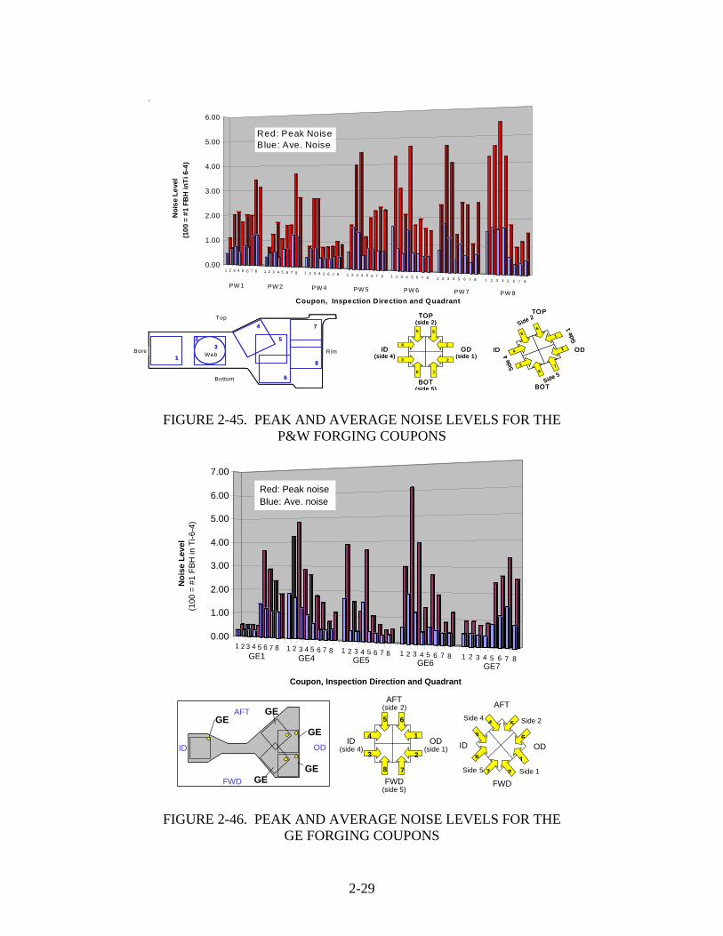
2-29

FIGURE 2-45. PEAK AND AVERAGE NOISE LEVELS FOR THE P&W FORGING COUPONS

FIGURE 2-46. PEAK AND AVERAGE NOISE LEVELS FOR THE GE FORGING COUPONS

1 2 3 4 5 6 7 8 1 2 3 4 5 6 7 8 1 2 3 4 5 6 7 8 1 2 3 4 5 6 7 8 1 2 3 4 5 6 7 8 0.00

1.00

2.00

3.00

4.00

5.00

6.00

7.00

Noi

se L

evel

(1

00 =

#1

FBH

in T

i-6-4

)

Coupon, Inspection Direction and Quadrant

GE1 GE7 GE6 GE5 GE4

US

GEGE

GE

GE

GE

AFT

FWD

ID ODOD

(side 1)

1

8 7

5

4

3 2

6

FWD(side 5)

ID(side 4)

AFT(side 2) AFT

OD ID

FWD

18

7

54

3

2

6

Side 1

Side 4 Side 2

Side 5

Red: Peak noise Blue: Ave. noise

Bore Web Rim1

23

4

5

6

7

8

Top

Bottom

OD(side 1)

1

8 7

5

4

3 2

6

BOT(side 5)

ID(side 4)

TOP(side 2)

TOP

ODID

BOT

1

87

5

4

3

2

6

Side

1

Side

4

Side 2

Side 5

1 2 3 4 5 6 7 8 1 2 3 4 5 6 7 8 1 2 3 4 5 6 7 8 1 2 3 4 5 6 7 8 1 2 3 4 5 6 7 8 1 2 3 4 5 6 7 8 1 2 3 4 5 6 7 8

0.00

1.00

2.00

3.00

4.00

5.00

6.00

Noi

se L

evel

(1

00 =

#1

FBH

inTi

6-4

) .

Coupon, Inspection Direction and Quadrant

PW 1PW 7PW 5PW 4PW 2 PW 6 PW 8

Red: Peak NoiseBlue: Ave. Noise

Bore Web Rim1

23

4

5

6

7

8

Top

Bottom

OD(side 1)

1

8 7

5

4

3 2

6

BOT(side 5)

ID(side 4)

TOP(side 2)

TOP

ODID

BOT

1

87

5

4

3

2

6

Side

1

Side

4

Side 2

Side 5

1 2 3 4 5 6 7 8 1 2 3 4 5 6 7 8 1 2 3 4 5 6 7 8 1 2 3 4 5 6 7 8 1 2 3 4 5 6 7 8 1 2 3 4 5 6 7 8 1 2 3 4 5 6 7 8

0.00

1.00

2.00

3.00

4.00

5.00

6.00

Noi

se L

evel

(1

00 =

#1

FBH

inTi

6-4

) .

Coupon, Inspection Direction and Quadrant

PW 1PW 7PW 5PW 4PW 2 PW 6 PW 8

Red: Peak NoiseBlue: Ave. Noise

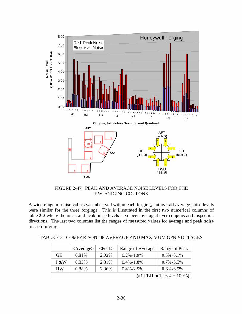
2-30

FIGURE 2-47. PEAK AND AVERAGE NOISE LEVELS FOR THE HW FORGING COUPONS

A wide range of noise values was observed within each forging, but overall average noise levels were similar for the three forgings. This is illustrated in the first two numerical columns of table 2-2 where the mean and peak noise levels have been averaged over coupons and inspection directions. The last two columns list the ranges of measured values for average and peak noise in each forging.

TABLE 2-2. COMPARISON OF AVERAGE AND MAXIMUM GPN VOLTAGES

<Average> <Peak> Range of Average Range of Peak GE 0.81% 2.03% 0.2%-1.9% 0.5%-6.1% P&W 0.83% 2.31% 0.4%-1.8% 0.7%-5.5% HW 0.88% 2.36% 0.4%-2.5% 0.6%-6.9%

(#1 FBH in Ti-6-4 = 100%)

1 2

3

4 5

6

7 8

9 10

AFT

FWD

OD

1 2

3

4 5

6

7 8

9 10

AFT

FWD

OD OD (side 1)

1

8 7

5

4

3 2

6

FWD(side 5)

ID(side 4)

AFT(side 2)

OD (side 1)

1

8 7

5

4

3 2

6

FWD(side 5)

ID(side 4)

AFT(side 2)

1 2 3 4 5 6 7 8 1 2 3 4 5 6 7 8 1 2 3 4 5 6 7 8 1 2 3 4 5 6 7 8 1 2 3 4 5 6 7 8 1 2 3 4 5 6 7 8 1 2 3 4 5 6 7 8 1 2 3 4 5 6 7 83 4 5 6 7 8 1 2 3 4 5 6 7 8 1 2 3 4 5 6 7 8 1 2 3 4 5 6 7 8

0.00

1.00

2.00

3.00

4.00

5.00

6.00

7.00

8.00

Coupon, Inspection Direction and Quadrant

H1 H8H4H3H2 H6 H5 H7

Noi

se L

evel

(1

00 =

#1

FBH

in

Ti 6

-4)

Red: Peak NoiseBlue: Ave. Noise

Honeywell Forging

2-31

2.2.2.2 Velocity and Attenuation Measurements.

For the forging flow line coupons, UT longitudinal-wave velocity and attenuation measurements were performed using the same procedures established in Phase I for rectangular billet coupons [16]. The basic experimental setups are shown in figure 2-48. Measurements were made through sides 1 and 2 of each specimen, generally corresponding to beam propagation in the radial and axial directions, respectively. The UT measurement system consisted of a Panametrics 5052 pulser/receiver, a Lecroy 9400A digitizing oscilloscope, a Testek water tank with a motorized XY scanning bridge, a manual gimble-gimble goniometer for adjusting the transducer orientation, and a personal computer to control scanning and data acquisition. The A-scans (radio frequency (RF) waveforms) required for the attenuation measurements were digitized at a 100-MHz sampling rate. Because the forging microstructure can sometimes act to steer the beam slightly, the front-wall echo was used to normalize the beam on the entry surface. That is, the two transducer orientation angles were adjusted so that the front-wall echo amplitude was maximized.

FIGURE 2-48. SETUPS USED FOR UT VELOCITY AND ATTENUATION MEASUREMENTS

(A 10-MHz, 1/4″ planar probe was used in each case. The water path was typically 5 cm.) The sound velocity near the center of the coupon was determined from the average time delay between the first three successive back-wall echoes, denoted BS1, BS2, and BS3, respectively, in figure 2-48. The time delay between two echoes was specifically defined as the time difference between the corresponding zero crossing points just preceding the dominant positive peaks in the RF waveforms. Results of the velocity measurements are shown in figure 2-49. Velocity variations were relatively small, with the measured values ranging from 0.617 to 0.622 cm/μsec, a spread of about 1%. Although the spread in measured values was small, some systematic variations were observed. For example, for the P&W coupons in figure 2-49, one sees that the difference between the velocities in the radial and axial directions tends to lessen as one moves from coupon HW1 (near the forging inside diameter (ID)) to coupon HW8 (near the forging outside diameter (OD)). It was also noted that the forging strain tends to decrease as one moves from the ID to the OD of the P&W forging (see figure 2-16).

Scan

-

Ti

Scan

-

Ti Ti Ti Fused Quartz Reference Ti 6 4 coupon

Scan

Attenuation Measurement

BS1 BS2 BS3

Velocity Measurement

2-32

FIGURE 2-49. MEASURED UT VELOCITIES FOR PROPAGATION IN THE RADIAL (THROUGH SIDE 1) AND AXIAL (THROUGH SIDE 2) DIRECTIONS OF THE

FORGING FLOW LINE COUPONS Unlike velocity, UT attenuation is typically a strong function of frequency. Attenuation-versus-frequency curves were measured by comparing the spectral amplitudes of the first back-wall echo in the Ti-6-4 specimen to a FQ reference block. (The method is described in detail in reference 16.) The macrostructure of engine Ti alloys acts to distort the pressure and amplitude profiles of a propagating sound beam. The details of these distortions vary from location to location within a coupon. As a consequence, back-wall amplitude C-scans tend to have a blotchy appearance rather than the uniform coloration of fine-grained metals. Stated in another way, the effective UT attenuation varies from point to point over relatively small distances. For this reason, the transducer was scanned in two dimensions above the specimen, and the attenuation values were measured at 100 or more locations within the central 1.5″ by 0.75″ area of each standard coupon. The quoted attenuation-versus-frequency curves for each specimen are, thus, area averages. Examples of measured average attenuation curves are shown in figure 2-50 for two of the coupons from the HW forging. The attenuation values are in Neper/cm units; if desired, multiply by 22.06 to change to dB/inch units. Measured values are most trustworthy in the frequency range from about 5 to 16 MHz where the spectral amplitudes of the back-wall echoes are largest. Similar attenuation-versus-frequency curves for the other forging flow line coupons can be found in appendix A. Forging inspections of Ti-6-4 engine disks with similar dimensions to those

Measured Longitudinal-Wave Sound Velocities for the Forging-Flowline Coupons in cm/microsec Units.

HW: Velocity Vs. Coupon Number

0.6140.6150.6160.6170.6180.6190.62

0.6210.6220.623

HW1 HW2 HW3 HW4 HW5 HW6 HW7 HW8Coupon Number

Velo

city

(cm

/us)

AxialRadial

GE: Velocity Vs. Coupon Number

0.615

0.616

0.617

0.618

0.619

0.62

0.621

0.622

GE1 GE4 GE5 GE6 GE7Coupon Number

Veloc

ity (c

m/us

)

AxialRadial

PW: Velocity Vs. Coupon Number

0.616

0.617

0.618

0.619

0.62

0.621

0.622

0.623

PW1 PW2 PW4 PW5 PW6 PW7 PW8Coupon Number

Velo

city

(cm

/us)

AxialRadial

Measured Longitudinal-Wave Sound Velocities for the Forging-Flowline Coupons in cm/microsec Units.

HW: Velocity Vs. Coupon Number

0.6140.6150.6160.6170.6180.6190.62

0.6210.6220.623

HW1 HW2 HW3 HW4 HW5 HW6 HW7 HW8Coupon Number

Velo

city

(cm

/us)

AxialRadial

GE: Velocity Vs. Coupon Number

0.615

0.616

0.617

0.618

0.619

0.62

0.621

0.622

GE1 GE4 GE5 GE6 GE7Coupon Number

Veloc

ity (c

m/us

)

AxialRadial

PW: Velocity Vs. Coupon Number

0.616

0.617

0.618

0.619

0.62

0.621

0.622

0.623

PW1 PW2 PW4 PW5 PW6 PW7 PW8Coupon Number

Velo

city

(cm

/us)

AxialRadial

2-33

studied here generally use 10-MHz transducers. Measured attenuation values at 10 MHz for this suite of forging flow line coupons are shown in figure 2-51 in dB/inch units. Figures 2-50 and 2-51 illustrate that attenuation variations across a forging can be considerable, with the attenuation being largest for radial propagation at some locations and largest for axial propagation at others. As will be discussed in the next section, certain aspects of the attenuation variations can be correlated with variations in forging strain.

FIGURE 2-50. MEASURED ATTENUATION-VERSUS-FREQUENCY CURVES FOR TWO COUPONS FROM THE HW Ti-6-4 FORGING

(Coupon HW1 (top panel) is from the mid-radius, aft region of the forging. Coupon HW7 (lower panel) is from the ID, forward region. The results

are shown for both radial and axial sound propagation.) 2.2.3 Relationship Between UT Properties and Forging Strain.

The property measurement coupons were also used to study the relationship between the UT properties and the local forging microstructures. The microstructural data consisted primarily of the macroetch photographs and the forging strain maps calculated using DEFORM. Although flow line directions in the macroetches can be readily discerned, it proved difficult to define and extract other quantitative measures of the flow lines (such as flow line density) from the photographs. Thus, it was decided that it might be more fruitful to work directly with the DEFORM outputs rather than the macroetch photographs.

Honeywell#7 Side1&2 Attenuation

0.00

0.05

0.10

0.15

0.20

0.25

0.30

0 2 4 6 8 10 12 14 16 18 20

Frequency (MHz)

Att

(Np/

cm)

Att_Side 1Att_Side2

Honeywell#1 Side1&2 Attenuation

0.00

0.03

0.06

0.09

0.12

0.15

0 2 4 6 8 10 12 14 16 18 20

Frequency (MHz)

Att

(Np/

cm)

Att_Side 1Att_Side2

radial

radial

axial

axial

Honeywell#7 Side1&2 Attenuation

0.00

0.05

0.10

0.15

0.20

0.25

0.30

0 2 4 6 8 10 12 14 16 18 20

Frequency (MHz)

Att

(Np/

cm)

Att_Side 1Att_Side2

Honeywell#1 Side1&2 Attenuation

0.00

0.03

0.06

0.09

0.12

0.15

0 2 4 6 8 10 12 14 16 18 20

Frequency (MHz)

Att

(Np/

cm)

Att_Side 1Att_Side2

radial

radial

axial

axial

2-34

FIGURE 2-51. MEASURED UT ATTENUATION VALUES AT 10 MHz FOR THE

FORGING FLOW LINE COUPONS (The results are shown for propagation in the radial direction

(through side 1) and axial direction (through side 2).) In Ti-6-4 billet materials, the ETC Phase I studies found that UT properties were correlated with the shapes and orientations of the large-scale microstructural elements known as macrograins. For example, backscattered grain noise levels tend to be largest when the beam travels perpendicular to the macrograin elongation direction, and effective attenuation values tend to be smallest for that beam propagation direction [16]. If little recrystallization occurs during the forging process, the macrograins in the billet will deform into associated macrograins in the forging, and these may largely control the UT properties of the forging. In billets, the macrograin elongation direction is predominantly along the billet axis. The situation will be more complicated in forgings since the local material deformation varies with position, as shown in figure 2-52.

For each OEM-supplied forging, the results of DEFORM calculations were given, showing how circular volume elements in the billet deform into elliptical elements in the forging. (See figures 2-7, 2-20, and 2-32.) However, since billet macrograins tend to be elongated along the billet axis, a more appropriate starting point for the current study would be DEFORM calculations in which the initial billet volume elements have elliptical cross sections. For the P&W and HW forgings, it was possible to work with the respective forging houses to carryout such calculations. However, similar calculations could not be obtained from Ladish, the source for the GE forging.

PW: Attenuation at 10MHz Bar Graph

00.20.40.60.8

11.21.41.61.8

PW#1 PW#2 PW#4 PW#5 PW#6 PW#7 PW#8

Coupon Number

Atte

nuat

ion

(dB/

inch

)

Axial(S2)Radial(S1)

GE: Attenuation at 10MHz Bar Graph

0

0.2

0.4

0.6

0.8

1

GE#1 GE#4 GE#5 GE#6 GE#7

Coupon Number

Atte

nuat

ion

(dB/

inch

)

Axial(S2)Radial(S1)

HW: Attenuation at 10MHz Bar Graph

0

0.5

1

1.5

2

2.5

3

HW#1 HW#2 HW#3 HW#4 HW#5 HW#6 HW#7 HW#8

Coupon Number

Atte

nuat

ion

(Np/

cm)

Axial(S2)Radial(S1)

Measured Longitudinal-Wave Attenuation Values for the Forging-Flowline Coupons at 10 MHz in dB/inch Units.

PW: Attenuation at 10MHz Bar Graph

00.20.40.60.8

11.21.41.61.8

PW#1 PW#2 PW#4 PW#5 PW#6 PW#7 PW#8

Coupon Number

Atte

nuat

ion

(dB/

inch

)

Axial(S2)Radial(S1)

GE: Attenuation at 10MHz Bar Graph

0

0.2

0.4

0.6

0.8

1

GE#1 GE#4 GE#5 GE#6 GE#7

Coupon Number

Atte

nuat

ion

(dB/

inch

)

Axial(S2)Radial(S1)

HW: Attenuation at 10MHz Bar Graph

0

0.5

1

1.5

2

2.5

3

HW#1 HW#2 HW#3 HW#4 HW#5 HW#6 HW#7 HW#8

Coupon Number

Atte

nuat

ion

(Np/

cm)

Axial(S2)Radial(S1)

Measured Longitudinal-Wave Attenuation Values for the Forging-Flowline Coupons at 10 MHz in dB/inch Units.

2-35

FIGURE 2-52. IN THE ABSENCE OF RECRYSTALLIZATION, THE SHAPES OF MACROGRAINS IN A FORGING WILL VARY WITH POSITION DUE TO

THE VARYING STRAIN LEVELS The results of the DEFORM calculations beginning with 5:1 elliptical elements in the billet (elongated parallel to the billet axis) are shown for the P&W and HW forgings in figures 2-53 and 2-54, respectively. One sees that both the elongations and orientations of the volume elements in the forgings are changed, compared to the predictions of the earlier DEFORM simulations. Note that the shapes and orientations of the volume elements in the forgings vary systematically with position. Also note that the forging volume elements tend to be elongated in the axial direction at some locations (e.g., near the forging OD) and tend to be elongated in the radial direction at other locations (e.g., near the forging ID). The elongations of physical macrograins in Ti forgings often exhibit a similar dependence on position, and it was assumed that the shapes and orientations of the volume elements in the DEFORM calculations approximate those of physical macrograins. In previous measurements of backscattered grain noise, it was found that noise levels varied significantly with location and inspection direction within forgings (see figures 2-45, 2-46, and 2-47). Some aspects of the noise variations appear to be well correlated with the forging macrograin shapes and orientations predicted by the DEFORM calculations. Consider figure 2-55 whose upper portion shows the strain diagram for the P&W Ti-6-4 forging, beginning with 5:1 ellipses in the billet. Superimposed on the diagram are the locations of seven rectangular property measurement coupons. Recall that noise measurements on each coupon were made in two directions for each of the four quadrants in the radial-axial plane. The lower portion of figure 2-55 lists the values of the noise anisotropy ratio (NAR) for each quadrant of each P&W coupon. This ratio, which is sometimes called, simply, the noise anisotropy, compares the average grain noise level measured for axial propagation (numerator of ratio) to the radial propagation (denominator). Ratio values near unity indicate that the backscattered noise level is similar for the two inspection directions. For tilted coupon PW4, the noise levels were measured at normal incidence, and the noise value through the upper or lower face (i.e., the nearly axial face) appears in the numerator.

Cast Ingot Reduced-Diameter Billet

Forging

“Macrograins”:large scale microstructure

Cast Ingot Reduced-Diameter Billet

Forging

“Macrograins”:large scale microstructure“Macrograins”:large scale microstructure

2-36

FIGURE 2-53. DEFORM CALCULATION FOR THE P&W FORGING, BEGINNING WITH

5:1 ELLIPTICAL VOLUME ELEMENTS IN THE BILLET

1

23

4

5

6

7 8

9

10

1

23

4

5

6

7 8

9

10

1

23

4

5

6

7 8

9

10

1

23

4

5

6

7 8

9

10

FIGURE 2-54. OUTPUT OF THE DEFORM CALCULATION FOR THE HW FORGING, BEGINNING WITH 5:1 ELLIPTICAL VOLUME ELEMENTS IN THE BILLET

(The approximate boundaries of the sonic shape and forging flow line coupons are also shown.)

Volume elements with 5:1 aspect ratio in the billet blank. (Full billet blank not shown)

Volume elements in the PW forging.

Volume elements with 5:1 aspect ratio in the billet blank. (Full billet blank not shown)

Volume elements in the PW forging.

2-37

FIGURE 2-55. STRAIN DIAGRAM FOR THE P&W Ti-6-4 FORGING, BEGINNING WITH 5:1 ELLIPSES IN THE BILLET ALIGNED WITH THE BILLET AXIS

Comparing the upper and lower portions of figure 2-55, one sees that (1) the forging volume elements tend to have about equal projections onto the two inspection directions in regions where the NAR is near unity; (2) the axial noise is larger than the radial noise (NAR > 1) in regions where the ellipses are elongated in the radial direction; and (3) the radial noise is larger than the axial noise (NAR < 1) in regions where the ellipses are elongated in the axial direction. Thus, overall, a coherent explanation of the noise anisotropy emerges if one assumes that forging macrograin geometries are primarily responsible for the noise, and that their shapes in the forging are determined by their shapes in the billet and the subsequent deformation during forging. The only major exception in figure 2-55 is for coupon PW5, which has relatively circular DEFORM elements throughout, but has a measured NAR that varies substantially from quadrant to quadrant. The macroetch revealed that this coupon is in a region with swirling flow lines; the relationship between noise and macrostructure may be more complicated there, or the DEFORM calculations may be less trustworthy in such a region. To carry the analysis further, tabulations were made of the macrograin shape and orientation characteristics, as calculated using DEFORM. As illustrated in figure 2-56, the computed elliptical volume elements were examined to determine (1) the length of the major axis, (2) the length of the minor axis, and (3) the (acute) orientation angle between the major axis and the radial direction of the forging (more generally, the direction normal to coupon sides 1 and 4). These quantities were measured near the center of each quadrant of each coupon, usually averaging the properties of neighboring ellipses to best estimate the values at the quadrant center. Attempts were then made to correlate attributes of the localized grain noise levels to the forging macrograin properties shown in figure 2-56. The best correlation discovered was between the NAR and the ellipse projection ratio defined in figure 2-57. Recall that the noise anisotropy is

1

24

5

6

7

8

1.55 1.62

1.67 1.78

1.82 2.05

2.10 2.36

0.95 0.91

0.58 0.63

1.52 1.20

0.52 0.44

0.45 0.40

0.90 0.68

2.10 0.82

0.58 0.23

0.37 0.26

0.33 0.25

or

or

Tabulation of Noise Anisotropyby Coupon Quadrant

(Axial Mean Noise / Radial Mean Noise)

1

24

5

6

7

81

24

5

6

7

81

24

5

6

7

8

1.55 1.62

1.67 1.78

1.82 2.05

2.10 2.36

0.95 0.91

0.58 0.63

1.52 1.20

0.52 0.44

0.45 0.40

0.90 0.68

2.10 0.82

0.58 0.23

0.37 0.26

0.33 0.25

1.55 1.62

1.67 1.78

1.82 2.05

2.10 2.36

0.95 0.91

0.58 0.63

1.52 1.20

0.52 0.44

0.45 0.40

0.90 0.68

2.10 0.82

0.58 0.23

0.37 0.26

0.33 0.25

or

or

or

or

Tabulation of Noise Anisotropyby Coupon Quadrant

(Axial Mean Noise / Radial Mean Noise)

2-38

defined as the ratio of the average GPN values for C-scans made from two orthogonal directions. The ellipse projection ratio, as the name implies, is the ratio of the projections of the strain ellipses onto the same two inspection directions. A correlation between these two ratios is not unexpected, since the backscattered noise level from a local region will depend, in part, on the cross section that the macrograins present to the sonic beam [22].

FIGURE 2-56. MEASURED PROPERTIES OF THE ELLIPTICAL MACROGRAINS IN FORGING STRAIN MAPS, AS CALCULATED USING DEFORM

Ave. Noise Seen From Axial Direction

Ave. Noise Seen From Radial DirectionNoise Anisotropy Ratio =

Y

X

Axial

RadialEllipse Projection Ratio= Y / X a

b

θ

Ave. Noise Seen From Axial Direction

Ave. Noise Seen From Radial DirectionNoise Anisotropy Ratio =

Y

X

Axial

RadialEllipse Projection Ratio= Y / X a

b

θ

FIGURE 2-57. DEFINITION OF THE ELLIPSE PROJECTION RATIO FOR A FORGING MACROGRAIN, AS CALCULATED USING DEFORM

Comparisons between the grain noise anisotropy ratio (from earlier C-scan noise measurements) and the ellipse projection ratio (from DEFORM calculations) are shown in figures 2-58 and 2-59 for the P&W and HW forgings, respectively. In each case, the assumed macrograins in the billet were 5:1 ellipsoids, elongated in the axial direction. There are four plotted points for each forging flow line coupon, corresponding to the four quadrants where measurements and analyses were made. For perfect correlation between grain noise anisotropy and the ellipse projection ratio, the plotted points in figures 2-58 or 2-59 would all lie along a diagonal line. This is approximately the case, although there is significant scatter about that ideal line, with the scatter being somewhat larger for the HW forging. The choice of 5:1 as an aspect ratio for the billet macrograins was a guess. If the billet aspect ratio is more properly chosen, one would expect that forging locations having circular macrograins would have a noise aspect ratio of unity, i.e.,

Ellipse properties directly measured from DEFORM outputs:Length of the major axis;Length of the minor axis;The (acute) orientation angle θ with the “radial”

direction as shown above.

θ“Radial” inspection direction(thru side 1 or 4) θ

6

These measurements were made at locations near the centers of the four quadrants of each coupon, indicated by the four white dots in the example at left (HW coupon # 6).

Ellipse properties directly measured from DEFORM outputs:Length of the major axis;Length of the minor axis;The (acute) orientation angle θ with the “radial”

direction as shown above.

θ“Radial” inspection direction(thru side 1 or 4) θ

θ“Radial” inspection direction(thru side 1 or 4) θ

66

These measurements were made at locations near the centers of the four quadrants of each coupon, indicated by the four white dots in the example at left (HW coupon # 6).

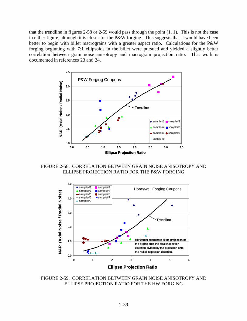
2-39

that the trendline in figures 2-58 or 2-59 would pass through the point (1, 1). This is not the case in either figure, although it is closer for the P&W forging. This suggests that it would have been better to begin with billet macrograins with a greater aspect ratio. Calculations for the P&W forging beginning with 7:1 ellipsoids in the billet were pursued and yielded a slightly better correlation between grain noise anisotropy and macrograin projection ratio. That work is documented in references 23 and 24.

FIGURE 2-58. CORRELATION BETWEEN GRAIN NOISE ANISOTROPY AND ELLIPSE PROJECTION RATIO FOR THE P&W FORGING

FIGURE 2-59. CORRELATION BETWEEN GRAIN NOISE ANISOTROPY AND ELLIPSE PROJECTION RATIO FOR THE HW FORGING

0.0

0.5

1.0

1.5

2.0

2.5

0.0 0.5 1.0 1.5 2.0 2.5 3.0 3.5 Ellipse Projection Ratio

NA

R (

Axi

al N

oise

/ R

adia

l Noi

se)

sample#1 sample#2 sample#4 sample#5 sample#6 sample#7 sample#8

P&W Forging Coupons

Trendline

0.0

0.5

1.0

1.5

2.0

2.5

0.0 0.5 1.0 1.5 2.0 2.5 3.0 3.5 Ellipse Projection Ratio

sample#1 sample#2 sample#4 sample#5 sample#6 sample#7 sample#8

P&W Forging Coupons

Trendline

0.0

1.0

2.0

3.0

4.0

5.0

0 1 2 3 4 5 6

Ellipse Projection Ratio

sample#1 sample#2sample#3 sample#4sample#6 sample#8sample#5 sample#7sample#9

Honeywell Forging Coupons

Horizontal coordinate is the projection of the ellipse onto the axial inspection direction divided by the projection onto the radial inspection direction.

Trendline

0.0

1.0

2.0

3.0

4.0

5.0

0 1 2 3 4 5 6

Ellipse Projection Ratio

NA

R (

Axi

al N

oise

/ R

adia

l Noi

se)

sample#1 sample#2sample#3 sample#4sample#6 sample#8sample#5 sample#7sample#9

Horizontal coordinate is the projection of the ellipse onto the axial inspection direction divided by the projection onto the radial inspection direction.

Trendline

2-40

A similar comparison between grain noise anisotropy and ellipse projection ratio was performed for the GE forging, although the only forging strain map available was that which assumed circular volume elements in the billet. The result is shown in figure 2-60. The measurement of ellipse properties was hampered by the quality of the DEFORM outputs provided by the forger (Ladish). In particular, for some high-deformation regions of the forging, it was not possible to accurately discern the dimensions of the individual ellipses in the strain map. Nonetheless, there is still a positive correlation for the GE forging.

FIGURE 2-60. CORRELATION BETWEEN GRAIN NOISE ANISOTROPY AND ELLIPSE PROJECTION RATIO FOR THE GE FORGING, BEGINNING WITH

CIRCULAR MACROGRAINS IN THE BILLET In summary, a good understanding of the noise anisotropy in Ti-6-4 forgings can be obtained by assuming that it is controlled by the shapes of the macrograins in the forging, which, in turn, arise from the macrograin shapes in the billet and the forging strain pattern. In particular, the noise level at a given forging location tends to be largest for the inspection direction in which the model macrograins present the largest cross-sectional area to the incident sound beam. This finding motivated further research to try to correlate absolute grain noise levels in forgings, rather than just noise ratios, to the DEFORM outputs. An effort was made to develop simulation models to predict the variation of the absolute UT grain noise level within a forging. The models treat the forging as an effective medium containing scattering elements (macrograins) whose mean properties vary systematically with position. One model input is the local geometry of a scattering element, including its elongation and orientation with respect to the incident UT beam; as before, the local macrograin geometry is calculated using DEFORM. Two additional model inputs are the mean volume of a scattering element (V) and a parameter (<(δC33) 2>) that quantifies the mean elastic property variation between neighboring scatterers. These latter two global inputs are assumed to be fixed throughout the forging and are deduced by fitting to a

0

1

2

3

4

5

0 2 4 6 8 10Ellipsoid Projection Ratio (Y/X)

Noi

se A

niso

trop

y

Sample #1Sample #4Sample #5Smaple #6Sample #7

GE Ti 6-4Forging Coupons

Trendline

0

1

2

3

4

5

0 2 4 6 8 10Ellipsoid Projection Ratio (Y/X)

Noi

se A

niso

trop

y

Sample #1Sample #4Sample #5Smaple #6Sample #7

GE Ti 6-4Forging Coupons

0

1

2

3

4

5

0 2 4 6 8 10Ellipsoid Projection Ratio (Y/X)

Noi

se A

niso

trop

y

Sample #1Sample #4Sample #5Smaple #6Sample #7

GE Ti 6-4Forging Coupons

Trendline

2-41

limited amount of experimental data. Mathematical details of the noise models that were developed for Ti engine forgings can be found in references [24, 25, and 26]. They are based on earlier work by Rose for the backscattered noise power scattered from randomly orientated, equiaxed, single-phase [27] and multiphase [28] polycrystals, and on the work of Han and Thompson [22] who extended Rose’s theory to the cases of duplex microstructures containing elongated microstructural features or texture. Appearing in the models is a commonly used measure of a microstructure’s noise-generating capability known as the backscattering power coefficient η, i.e., the differential scattering cross section per unit volume in the backward direction [27 and 28]. Here, it was preferred to use the square root of η, the grain noise FOM, since it is directly proportional to the noise voltage observed on an oscilloscope during UT inspection. The grain noise FOM-versus-frequency curve, which depends only on the metal microstructure and beam propagation direction, is measured by comparing the average spectral components of noise A-scans to those of a front-wall or back-wall reference signal. The grain-noise FOM and its measurement are described in reference 16 and the references cited therein. The forging noise model comes in two forms, a simpler one, which ignores the effects on microstructural texture (preferentially oriented crystalline axes), and a more complex model, which treats texture. To develop and test the noise models, the P&W Ti-6-4 forging was chosen because a faster turn around of DEFORM calculations was available. Beginning with 7:1 ellipsoidal elements in the billet, the usual DEFORM strain map was generated to determine the shapes and orientations of the macrograins within the forging, with these serving as one class of noise model inputs. For the untextured model, the remaining two global parameters (macrograin volume V and elastic constant anisotropy factor (<(δC33)2>) were obtained by comparing predicted FOM-versus-frequency curves to the measured curves for one quadrant of one forging flow line coupon, i.e., the quadrant closest to sides 1 and 5 of coupon PW8 (located in the rim region of the forging). The two model parameters were adjusted to maximize the agreement between the measured and predicted FOM curves, as shown in figure 2-61. The optimal average scatterer volume was estimated as V = 1.328e-06 cm3, and the optimal elastic property variation factor was estimated as <(δC33) 2> = 9.75 GPa2. Once the model parameters were determined, backscattered noise predictions could be made for other locations and inspection directions throughout the forging. Examples of such predictions are shown in figure 2-62 for inspections in the axial and radial directions of coupon PW2, located in the web region of the forging. Note that coupons PW2 and PW8 have very different local flow line geometries, as shown in figure 2-62. Also note that for PW8, the measured noise level is highest for radial propagation, while for PW2, it is highest for axial propagation. This reversal of noise directionality is well-predicted by the model. The noise model was also used to predict the average GPN amplitudes (relative to the FBH reference), which were previously measured for C-scans over each quadrant of each P&W coupon. The procedure used to make such predictions is described in reference 24. It makes use of the fact that, to a good first approximation, the average GPN amplitude within a quadrant will be proportional to the average FOM value near the center frequency of the transducer. For selected coupons, measured FOM and GPN data were both available, and these were used to find

2-42

FIGURE 2-61. MEASURED AND FITTED GRAIN NOISE FOM CURVES FOR THE LOWER RIGHT QUADRANT OF FORGING COUPON PW8, ASSUMING MACROGRAINS

WITH 7:1 ASPECT RATIOS IN THE BILLET

FIGURE 2-62. MEASURED AND PREDICTED GRAIN NOISE FOM CURVES FOR INSPECTIONS THROUGH SIDES 4 AND 5 OF FORGING COUPON PW2, BASED ON

MODEL PARAMETERS DEDUCED BY FITTING TO NOISE DATA FROM COUPON PW8

Bore Web

RimSide 2

Side 5

Side 4 Side 18

Minmizing the Sum of Errors Square to fit the Exp. V=1.328E-06cm^3, <deltaC^2>=9.75 Gpa^2

0.000

0.005

0.010

0.015

0.020

0.025

0.030

0.035

4 6 8 10 12 14 16Frequency (MHz)

FOM

(1/c

m^0

.5)

side1 Exp.Side 5 Exp.side1_fittingSide5 Fitting

Bore Web

RimSide 2

Side 5

Side 4 Side 18

Bore Web

RimSide 2

Side 5

Side 4 Side 1

Bore Web

Rim

Bore Web

Rim

Bore Web

RimSide 2

Side 5

Side 4 Side 18

Minmizing the Sum of Errors Square to fit the Exp. V=1.328E-06cm^3, <deltaC^2>=9.75 Gpa^2

0.000

0.005

0.010

0.015

0.020

0.025

0.030

0.035

4 6 8 10 12 14 16Frequency (MHz)

FOM

(1/c

m^0

.5)

side1 Exp.Side 5 Exp.side1_fittingSide5 Fitting

The Predict FOM on PW #2 S5&S4 V=1.328E-06cm^3, deltaC^2=9.75 GPa^2

0.000

0.005

0.010

0.015

0.020

0.025

0.030

4 6 8 10 12 14 16Freque ncy (M Hz)

FO

M (1

/cm

^0.5

)

side4_Expside4_predictionSide5 Exp.Side5_Prediction

Bore Web

Rim

28

Side 2

Side 5

Side 4Side 1

Side 2

Side 5

Side 4 Side 1

FitPrediction

The Predict FOM on PW #2 S5&S4 V=1.328E-06cm^3, deltaC^2=9.75 GPa^2

0.000

0.005

0.010

0.015

0.020

0.025

0.030

4 6 8 10 12 14 16Freque ncy (M Hz)

FO

M (1

/cm

^0.5

)

side4_Expside4_predictionSide5 Exp.Side5_Prediction

Bore Web

Rim

28

Side 2

Side 5

Side 4Side 1

Side 2

Side 5

Side 4 Side 1

FitPrediction

Bore Web

Rim

28

Side 2

Side 5

Side 4Side 1

Side 2

Side 5

Side 4 Side 1

Bore Web

Rim

Bore Web

Rim

28

Side 2

Side 5

Side 4Side 1

Side 2

Side 5

Side 4 Side 128

Side 2

Side 5

Side 4Side 1

Side 2

Side 5

Side 4Side 1

Side 2

Side 5

Side 4 Side 1

Side 2

Side 5

Side 4 Side 1

FitPrediction

2-43

the scaling factor, relating average GPN to FOM at 10 MHz. Using this scaling factor, GPN amplitudes could then be predicted from the model FOM curves predicted for each coupon quadrant. Predicted GPN amplitudes are compared with the experiment for the P&W forging in figure 2-63, using the untextured version of the noise model. Each forging coupon yielded eight plotted points, corresponding to the combination of four quadrants and two inspection directions (axial and radial). The simplified model treatment ignores the fact that UT attenuation varies throughout the forging, and effectively ignores the frequency dependence of FOM. Nonetheless, one observes a good correlation between measured and predicted GPN amplitudes, which each vary by a factor of 5 within the forging. If the model were exact, the points in figure 2-63 would all lie along a diagonal line through the plot region. The largest departures from this ideal situation generally occurred for coupons 5 and 6, where, as noted earlier, the macroetch reveals flow lines having a swirling appearance.

FIGURE 2-63. MEASURED AND PREDICTED AVERAGE GPN AMPLITUDES FOR THE VARIOUS QUADRANTS OF THE FORGING FLOW LINE COUPONS FROM THE

P&W FORGING (RELATIVE TO A VALUE OF 100 FOR THE #1 FBH IN THE IN100 REFERENCE BLOCK)

Recall that in addition to the rectangular coupons, one cylindrical coupon was cut from a high-strain region of each OEM-supplied forging. Backscattered noise measurements were performed using these three cylindrical coupons to investigate the variation of noise with rotation angle. Figure 2-64 shows the GPN C-scan obtained by stacking the three 1.25″ diameter coupons atop one another and performing a rotational-axial scan using a 5-MHz cylindrically focused transducer. For a full rotation of each of the cylindrical forging coupons, one observes a pattern of low-high-low-high noise amplitude.

Pre d icte d GPN Vs. Expe r ime ntal GPN (Normalize d by #1FBH in 1N100 ),

V=1.328E-06 cm^3, <de ltaC^2>=9.75GPa^2

0.0

1.0

2.0

3.0

4.0

5.0

6.0

0.0 1.0 2.0 3.0 4.0 5.0 6.0Norm a lize d GPN by Pre diction

No

rmal

ized

GP

N f

rom

Exp

erim

PW#1 PW#2 PW#4PW#5 PW#6 PW#7PW#8

2-44

FIGURE 2-64. GATED-PEAK GRAIN NOISE C-SCAN IMAGE RESULTING FROM A ROTATIONAL-AXIAL SCAN OF THE CYLINDRICAL COUPONS FROM THE

HIGH-STRAIN REGIONS OF THE THREE Ti-6-4 FORGINGS (A cylindrically focused, 0.5″ diameter, 5-MHz transducer having a nominal 4-cm

focal length was used. The inspection water path was 2.4 cm.) The cylindrical coupon from the P&W forging was used to further test the two-parameter (untextured) noise model. Measured and predicted angular noise profiles are shown in figure 2-65. The model curve is the predicted FOM profile (at 10 MHz) scaled to have about the same peak amplitude as the experimental curve. As before, the experimental and model quantities are expected to be approximately proportional to one another, although the scaling factor will be different from that used earlier because of the effect of the curved entry surface. The model (in this case, based on 7:1 ellipsoidal volume elements in the billet) successfully predicts the overall shape of the angular profile, but with somewhat sharper peaks than the experiment. The model tests, using the cylindrically focused transducer, are discussed in reference 24. The version of the grain noise model used in figure 2-61 through 2-65 did not account for metal texture that is known to be generated by forging processes [25]. Large deformations during forging are expected to cause partial alignment of crystallites by slip, twinning, or their combination. Such deformation-dependent texture will cause the elastic property variability factor, <δC332>, to vary with position inside the forging. A second version of the model formalism was developed, which accounts for both strain and texture, and model predictions were similarly performed and compared with experiment. This more complex model is discussed in references 25 and 26. Figure 2-66, taken from reference 25, compares measured and predicted absolute grain noise levels in the P&W forging, in the style of figure 2-63. Taken

PW3

GE2

HW10

Degrees

PW#3

GE#2

HW#10

PW3

GE2

HW10

Degrees

PW#3

GE#2

HW#10

PW#3

GE#2

HW#10

PW#3

GE#2

HW#10

2-45

as a whole, the collection of plotted points in figure 2-66, which used a texture effect, lie closer to the ideal diagonal line (representing perfect correlation between model and experiment) than figure 2-63 (noise model without a texture effect).

FIGURE 2-65. COMPARISONS OF MEASURED AND PREDICTED ANGULAR PROFILES FOR BACKSCATTERED GRAIN NOISE IN THE CYLINDRICAL

COUPON FROM THE WEB REGION OF THE P&W Ti-6-4 FORGING

00 3600

C-scan Image of Gated-Peak Noise (GPN) from cylindrical coupon PW3

Bore Web

Rim

3Angle

Angle Between Macrograin Major Axis and Inspection Direction (Degrees)

Ang

ular

Pro

files

of M

easu

red

Aver

age

Gat

ed-

Peak

Noi

se a

nd P

redi

cted

FO

M a

t 5 M

Hz.

Model

Experiment

00 3600

C-scan Image of Gated-Peak Noise (GPN) from cylindrical coupon PW3

00 360000 3600

C-scan Image of Gated-Peak Noise (GPN) from cylindrical coupon PW3

Bore Web

Rim

3Angle

Bore Web

Rim

3

Bore Web

Rim

Bore Web

Rim

3Angle

Angle Between Macrograin Major Axis and Inspection Direction (Degrees)

Ang

ular

Pro

files

of M

easu

red

Aver

age

Gat

ed-

Peak

Noi

se a

nd P

redi

cted

FO

M a

t 5 M

Hz.

Model

Experiment

2-46

FIGURE 2-66. MEASURED AND PREDICTED AVERAGE GATED-PEAK GRAIN NOISE AMPLITUDES FOR VARIOUS QUADRANTS OF THE FORGING FLOW

LINE COUPONS FROM THE P&W FORGING (Absolute noise amplitudes are relative to a value of 100

for the #1 FBH in the IN100 reference block.)

The following briefly summarizes the model development work performed to better understand grain noise variability within forgings. A fairly simple two-parameter model was first developed that can predict grain noise variations within Ti-6-4 forgings. The model approximates the forging microstructure as an effective medium containing scattering elements, referred to here as macrograins, in which the average macrograin volume is constant throughout the forging, and the crystalline axes of the grains are randomly oriented relative to one another. The shapes and orientations of the macrograins were deduced from DEFORM simulations of material strain and, consequently, vary throughout the forging. The two global (constant) model parameters, the mean volume of the scattering elements and the elastic property variability, were obtained by fitting to noise data for one particular region of the P&W Ti-6-4 forging. Model testing was then done by comparing predictions with experimental data for (1) FOM-versus-frequency curves for selected rectangular coupons, (2) mean GPN amplitudes within the four quadrants of each of the seven rectangular coupons cut from different regions of the forging, and (3) angular dependence of grain noise for one cylindrical coupon cut from the web region of the forging. Reasonable agreement between experiment and theory was achieved, indicating the model captured the main factors that control the variability of backscattered grain noise within the forging. The simple two-parameter model neglects metal texture that develops in high-strain regions of the forging (i.e., preferentially oriented crystalline axes, as indicated by velocity anisotropy). A more complex model that treats texture effects was developed, which appears to produce slightly better agreement with experiment. (See references 24, 25, and 26 for more details.) Note that these modeling efforts, to relate UT grain to forging strain, are a work-in-progress, and the results in the present report are only preliminary. It is anticipated that future updated results should be available in the

Measured and Predicted Gated Peak Noise in P&W Forging [ V=1.167E-06 cm^3, <deltaC^2_Opt>=14.25GPa^2 ]

0.0

1.0

2.0

3.0

4.0

5.0

6.0

0.0 1.0 2.0 3.0 4.0 5.0 6.0Predicted GPN Level

Expe

rimen

tal G

PN L

evel

PW#1 PW#2 PW#4PW#5 PW#6 PW#7PW#8

2-47

PhD thesis of Linxiao Yu [26] and in planned publications in the open scientific literature, which will be based on that thesis. For the forging flow line coupons, the primary interest was the study of noise variability, since, in practice, backscattered grain noise is generally the key UT property that determines flaw size detection limits. However, noise and velocity variations in the forgings and their relationship to forging strain were examined. As with backscattered noise, there were correlations between the attenuation and velocity anisotropies and various measures of the forging strain, as shown in figures 2-67 and 2-68. In analogy with backscattered noise, the attenuation anisotropy for a given coupon was defined as the ratio of the attenuation values in the axial and radial directions at some fixed frequency. Then the anisotropy ratio was compared to a dimensionless measure of the total strain developed during forging at the location of the coupon. The strain measure used in figures 2-67 and 2-68 was based on the DEFORM calculations, which showed how circular volume elements in the radial-axial plane of the billet were deformed into elliptical elements in the radial-axial plane of forging. The circular element calculations were used because they were available for all three forgings. For these two figures, the simple ratio of the major to minor ellipse axes (averaged over the coupon volume) was used as the measure of the deformation strain amplitude, and noise and attenuation values for a given propagation direction were averaged over the coupon quadrants. As shown in figure 2-67, both noise and attenuation anisotropies were found be correlated to deformation strain amplitude, but in opposite manners. At sites where the radial noise exceeded the axial noise, it was generally found that the axial attenuation exceeded the radial attenuation. A similar behavior was observed in the ETC Phase I studies of Ti-6-4 billet coupons and was traced to the shapes of the macrograins in billets [16]. The current work further indicates that macrograin shape and orientation also play an important role in determining the UT attenuation variations within forgings. The velocity anisotropy of the forging coupons was also examined and found to be correlated with forging strain amplitude, as shown in figure 2-68, although the degree of correlation was somewhat less than for noise or attenuation. The quantity plotted on the vertical axis in figure 2-68 is the percentage difference in velocities measured in the axial and radial directions. The horizontal axis again displays the ratio of the major to minor ellipse axes of the deformed volume elements averaged over the coupon in question. Developing models to predict velocity and attenuation variations within forgings would be an interesting topic for future research. The measured UT properties of the forging flow line coupons and the related forging strain maps reported herein can serve as data for guiding the development and testing of such models. 2.2.4 Identification of the High-Noise Coupons and Measurements of Grain Noise FOM.

When designing UT inspections of forgings, the high-noise regions are of chief interest since the elevated grain noise levels there can mask echoes from small or weakly reflecting defects. For this reason, additional UT measurements were performed for the highest-noise coupon from each OEM-supplied forging. These additional measurements included determination of the attenuation and the backscattered grain noise capacity (FOM), both of which are frequency-dependent quantities determined solely by the metal microstructure. Although all the forging flow line coupons were cut from high-noise quadrants of their respective forgings, some coupons had higher grain noise levels than others. The highest-noise coupon from each forging was identified by comparing backscattered noise C-scans, such as those contained in appendix A. All the rectangular coupons were examined, including a few that were smaller than the standard

2-48

size (1.25″ by 1.25″ by 2.0″). The highest-noise coupons from each forging were all found to be of standard size, i.e., coupons GE6, PW8, and HW5. The locations of these coupons within their respective forgings and the inspection directions producing the highest grain noise levels are illustrated in figures 2-69 through 2-71. Backscattered noise C-scan images are also shown.

FIGURE 2-67. RELATIONSHIPS BETWEEN NOISE ANISOTROPY, ATTENUATION ANISOTROPY, AND TOTAL FORGING STRAIN FOR COUPONS CUT FROM VARIOUS

LOCATIONS IN OEM-SUPPLIED Ti-6-4 FORGED ENGINE DISKS

FIGURE 2-68. RELATIONSHIP BETWEEN VELOCITY ANISOTROPY AND LOCAL

TOTAL FORGING STRAIN FOR Ti-6-4 FORGING FLOW LINE COUPONS

Noise Anisotropy =

Noise in Axial Dir.

Noise in Radial Dir.

Atten. Anisotropy =

Atten. (10 MHz) in Axial Dir.

Atten. (10 MHz) in Radial Dir.

Attenuation Anisotropy Vs. Total Strain

0

0.5

1

1.5

2

2.5

0 2 4 6 8 10

Deformation Strain

Atte

nuat

ion

Ani

sotr

opy

HW CouponsGE CouponsPW Coupons

Noise Anisotropy Vs. Total Strain

0

1

2

3

4

5

0 2 4 6 8 10

Deformation Strain

Noi

se A

niso

trop

y

HW CouponsGE CouponsPW Coupons

Noise Anisotropy Vs. Attenuation Anisotropy

0

1

2

3

4

5

0 0.5 1 1.5 2 2.5

Attenuation Anisotropy

Noi

se A

niso

trop

y

HW CouponsGE CouponsPW Coupons

0.0

0.1

0.2

0.3

0.4

0.5

0.6

0.7

0 2 4 6 8 10Average Strain (Y/X)

Perc

enta

ge V

eloc

ity

Varia

tion

from

Rad

ial t

o A

xial

HW CouponsGE CouponsPW Coupons

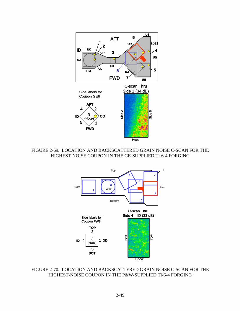
2-49

FIGURE 2-69. LOCATION AND BACKSCATTERED GRAIN NOISE C-SCAN FOR THE HIGHEST-NOISE COUPON IN THE GE-SUPPLIED Ti-6-4 FORGING

FIGURE 2-70. LOCATION AND BACKSCATTERED GRAIN NOISE C-SCAN FOR THE HIGHEST-NOISE COUPON IN THE P&W-SUPPLIED Ti-6-4 FORGING

Side labels for Coupon GE6

24

5 1(Hoop)

AFT

FWD

ID OD3

US

UG

UR

UPUO

UZ

UMUL

UK

UJ

UH

US

12

4

58

3

6

7

AFT

FWD

IDOD

C-scan ThruSide 1 (34 dB)

Hoop

Sid

e 2

Sid

e 5

Side labels for Coupon GE6

24

5 1(Hoop)

AFT

FWD

ID OD324

5 1(Hoop)

AFT

FWD

ID OD3

US

UG

UR

UPUO

UZ

UMUL

UK

UJ

UH

US

12

4

58

3

6

7

AFT

FWD

IDOD

US

UG

UR

UPUO

UZ

UMUL

UK

UJ

UH

US

12

4

58

3

6

7

AFT

FWD

IDOD

US

UG

UR

UPUO

UZ

UMUL

UK

UJ

UH

US

12

4

58

3

6

7

AFT

FWD

IDOD

C-scan ThruSide 1 (34 dB)

Hoop

Sid

e 2

Sid

e 5

Bore Web Rim1

23

4

5

6

7

8

Top

Bottom

Side labels for Coupon PW8

2

4

5

1(Hoop)

TOP

BOT

ID OD3

C-scan ThruSide 4 = ID (33 dB)

TOP

BO

T

HOOP

Bore Web Rim1

23

4

5

6

7

8

Top

Bottom

Bore Web Rim1

23

4

5

6

7

8

Top

Bottom

Side labels for Coupon PW8

2

4

5

1(Hoop)

TOP

BOT

ID OD3

Side labels for Coupon PW8

2

4

5

1(Hoop)

TOP

BOT

ID OD3

C-scan ThruSide 4 = ID (33 dB)

TOP

BO

T

HOOP

C-scan ThruSide 4 = ID (33 dB)

TOP

BO

T

HOOP

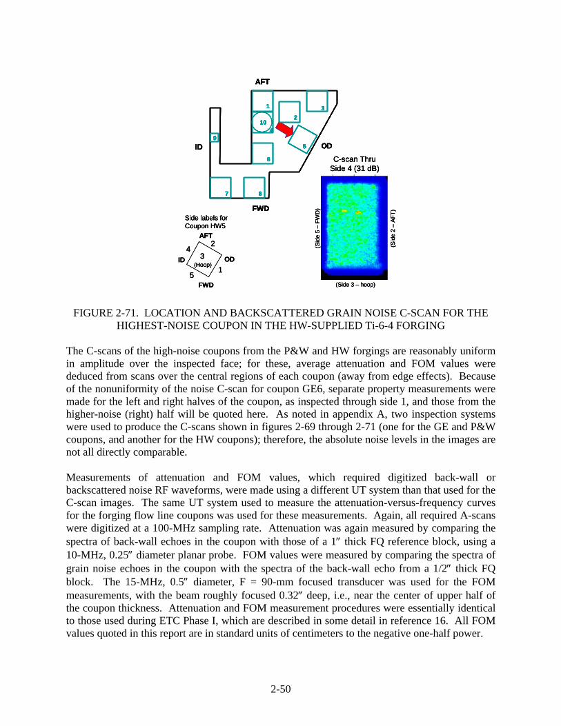
2-50

FIGURE 2-71. LOCATION AND BACKSCATTERED GRAIN NOISE C-SCAN FOR THE HIGHEST-NOISE COUPON IN THE HW-SUPPLIED Ti-6-4 FORGING

The C-scans of the high-noise coupons from the P&W and HW forgings are reasonably uniform in amplitude over the inspected face; for these, average attenuation and FOM values were deduced from scans over the central regions of each coupon (away from edge effects). Because of the nonuniformity of the noise C-scan for coupon GE6, separate property measurements were made for the left and right halves of the coupon, as inspected through side 1, and those from the higher-noise (right) half will be quoted here. As noted in appendix A, two inspection systems were used to produce the C-scans shown in figures 2-69 through 2-71 (one for the GE and P&W coupons, and another for the HW coupons); therefore, the absolute noise levels in the images are not all directly comparable. Measurements of attenuation and FOM values, which required digitized back-wall or backscattered noise RF waveforms, were made using a different UT system than that used for the C-scan images. The same UT system used to measure the attenuation-versus-frequency curves for the forging flow line coupons was used for these measurements. Again, all required A-scans were digitized at a 100-MHz sampling rate. Attenuation was again measured by comparing the spectra of back-wall echoes in the coupon with those of a 1″ thick FQ reference block, using a 10-MHz, 0.25″ diameter planar probe. FOM values were measured by comparing the spectra of grain noise echoes in the coupon with the spectra of the back-wall echo from a 1/2″ thick FQ block. The 15-MHz, 0.5″ diameter, F = 90-mm focused transducer was used for the FOM measurements, with the beam roughly focused 0.32″ deep, i.e., near the center of upper half of the coupon thickness. Attenuation and FOM measurement procedures were essentially identical to those used during ETC Phase I, which are described in some detail in reference 16. All FOM values quoted in this report are in standard units of centimeters to the negative one-half power.

1

23

4

5

6

7 8

9

10

AFT

FWD

OD

1

23

4

5

6

7 8

9

10

AFT

FWD

ODID

Side labels for Coupon HW5

2

5

4

1(Hoop)

AFT

FWD

ID OD3

C-scan ThruSide 4 (31 dB)

(Side 3 – hoop)

(Sid

e 2

–AF

T)

(Sid

e 5

–FW

D)

1

23

4

5

6

7 8

9

10

AFT

FWD

OD

1

23

4

5

6

7 8

9

10

AFT

FWD

ODID

1

23

4

5

6

7 8

9

10

AFT

FWD

OD

1

23

4

5

6

7 8

9

10

AFT

FWD

ODID

Side labels for Coupon HW5

2

5

4

1(Hoop)

AFT

FWD

ID OD3

Side labels for Coupon HW5

2

5

4

1(Hoop)

AFT

FWD

ID OD3

C-scan ThruSide 4 (31 dB)

(Side 3 – hoop)

(Sid

e 2

–AF

T)

(Sid

e 5

–FW

D)

C-scan ThruSide 4 (31 dB)

(Side 3 – hoop)

(Sid

e 2

–AF

T)

(Sid

e 5

–FW

D)

2-51

The velocity and attenuation measurements (averaged over entry surfaces) that were performed for all the standard-sized forging flow line coupons. The results for the high-noise coupons PW8 and HW5 were checked by repeating the measurements, and for coupon GE6, separate attenuation measurements were taken for the left and right halves of the side 1 entry surface. A power-law fit to the attenuation data for each high-noise coupon was then performed, as illustrated in figure 2-72 for the HW case. In that figure, average measured attenuation values are shown for scans over two areas of the coupon: a full scan region (central region measuring 1.5″ by 0.75″ at the entry surface) and a reduced-area region (central 1.25″ by 0.50″). The measured attenuation values are very similar for the two regions. For GE6, there was little difference in measured velocity or attenuation for the two halves of the coupon, but the noise FOM values were found to be quite different, as expected from the noise C-scan image.

FIGURE 2-72. MEASURED ATTENUATION VALUES AND POWER-LAW FIT FOR THE HW HIGH-NOISE COUPON

Because the microstructure typically varies with depth, FOM values were deduced for a series of depths by using time gates with different centers and durations. The results of the procedure are shown in figures 2-73 through 2-75 for the high-noise HW coupon. Figure 2-73 shows the root mean squared (rms) grain noise level as a function of time for the scan above side 4. The rms noise level (deduced from noise A-scans described in references 16 and 29) depicts the manner in which the absolute grain noise level varies with observation time or, equivalently, with depth within the specimen. For uniform microstructures, the rms noise level tends to peak near the round-trip travel time to the focal zone. Six time gates spanning different depth zones are also shown in figure 2-73. FOM-versus-frequency curves were deduced separately from the grain noise echoes within each of these gates, and the results are shown in figure 2-74. The FOM extraction procedure [16] requires knowledge of the attenuation-versus-frequency curve, and the measured attenuation curve (which is actually an average over the coupon thickness) was used in the analysis. One sees in figure 2-74 that the deduced FOM curve depends somewhat on the time gate used. This dependence is believed to be primarily due to the forging microstructure

0.00

0.01

0.02

0.03

0.04

0.05

4 6 8 10 12 14 16 18Frequency (MHz)

Atte

nuat

ion

(Nep

ers/

cm)

Full scan region

Reduced scan region

Power Law Fitfit is 0.00082 x freq1.343

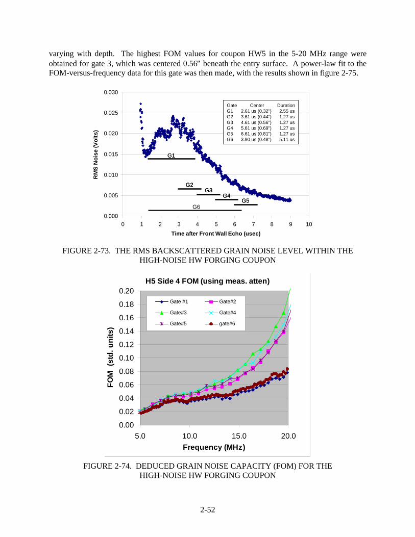
2-52

varying with depth. The highest FOM values for coupon HW5 in the 5-20 MHz range were obtained for gate 3, which was centered 0.56″ beneath the entry surface. A power-law fit to the FOM-versus-frequency data for this gate was then made, with the results shown in figure 2-75.

FIGURE 2-73. THE RMS BACKSCATTERED GRAIN NOISE LEVEL WITHIN THE HIGH-NOISE HW FORGING COUPON

FIGURE 2-74. DEDUCED GRAIN NOISE CAPACITY (FOM) FOR THE

HIGH-NOISE HW FORGING COUPON

0.000

0.005

0.010

0.015

0.020

0.025

0.030

0 1 2 3 4 5 6 7 8 9 10Time after Front Wall Echo (usec)

RM

S N

oise

(Vol

ts)

Gate Center DurationG1 2.61 us (0.32”) 2.55 usG2 3.61 us (0.44”) 1.27 usG3 4.61 us (0.56”) 1.27 usG4 5.61 us (0.69”) 1.27 usG5 6.61 us (0.81”) 1.27 usG6 3.90 us (0.48”) 5.11 us

G4G5

G1

G2G3

G60.000

0.005

0.010

0.015

0.020

0.025

0.030

0 1 2 3 4 5 6 7 8 9 10Time after Front Wall Echo (usec)

RM

S N

oise

(Vol

ts)

Gate Center DurationG1 2.61 us (0.32”) 2.55 usG2 3.61 us (0.44”) 1.27 usG3 4.61 us (0.56”) 1.27 usG4 5.61 us (0.69”) 1.27 usG5 6.61 us (0.81”) 1.27 usG6 3.90 us (0.48”) 5.11 us

G4G4G5G5

G1G1

G2G2G3G3

G6

H5 Side 4 FOM (using meas. atten)

0.00

0.02

0.04

0.06

0.08

0.10

0.12

0.14

0.16

0.18

0.20

5.0 10.0 15.0 20.0Frequency (MHz)

FOM

(st

d. u

nits

)

Gate #1 Gate#2

Gate#3 Gate#4

Gate#5 gate#6

2-53

FIGURE 2-75. MEASURED FOM CURVE AND ASSOCIATED POWER-LAW FIT FOR

THE HIGHEST-NOISE DEPTH ZONE WITHIN THE HIGH-NOISE COUPON FROM THE HW Ti-6-4 FORGING

Similar analyses were performed for the highest-noise coupons from the GE and P&W forgings. Measured FOM-versus-frequency curves for the same set of six depth zones are shown in figure 2-76. Again, for each coupon, a power-law fit was made to the FOM curve for the depth zone having the largest FOM values. The results for the three high-noise coupons are compared in table 2-3 for the depth zone having the highest noise capacity. Listed noise FOM values are conservative in the sense that they are the highest values measured for any depth zone in these coupons. The peak grain noise FOM value was largest for the HW forging and roughly similar for the GE and P&W forgings. Note that the differences in FOM values in table 2-3 are greater than the corresponding differences in average noise values listed in table 2-2. This is chiefly because, in the survey measurements leading to table 2-2, only GPN amplitudes were measured (relative to an FBH reference), and the focal spot of the transducer was not necessarily located in the depth zone where the noise capacity was greatest. For table 2-3 however, noise A-scan data were analyzed in a manner that identified the depth zone with the greatest noise capacity. In addition, the FOM measurement procedure accounts for the differences in attenuation of the various coupons, which also affect absolute grain noise levels. The UT properties listed in table 2-3 were originally compiled to support PoD computations planned under the suspended PoD of forgings subtask. These properties can be used as inputs to computer models that simulate UT inspections of forgings and estimate S/N ratios for defects of various types. Examples of such simulations for one proposed forging inspection scheme can be found in an article written for the 2001 QNDE conference held in Brunswick, Maine [23].

H5 Side 4 FOM (using meas. atten)

y = 0.00415x1.07820

0.00

0.01

0.02

0.03

0.04

0.05

0.06

0.07

0.08

0.09

0.10

4 6 8 10 12 14 16Frequency (MHz)

FOM

(st

d. u

nits

)

Gate#3

Pow er (Gate#3)

2-54

FIGURE 2-76. MEASURED GRAIN NOISE FOM VALUES, AS FUNCTIONS OF FREQUENCY, FOR THE GE AND P&W HIGH-NOISE FORGING COUPONS

TABLE 2-3. COMPARISON OF UT PROPERTIES FOR THE HIGH-NOISE COUPONS

FROM THE P&W, GE, AND HW Ti-6-4 FORGINGS

P&W GE HW Velocity (cm/μsec): 0.622 0.618 0.621 Density (gm/cc): 4.43 4.43 4.43 Attenuation power law*: 6.83E-4*freq.1.79 4.31E-5*freq.2.26 8.20E-*freq.1.34 Attenuation at 10 MHz: 0.93 dB/inch 0.17 dB/inch 0.40 dB/inch FOM power law*: 1.61E-3*freq.1.25 2.93E-3*freq.0.896 4.15E-3*freq.1.078 Meas. FOM at 10 MHz: 0.027 0.021 0.047

*For power laws, units are N/cm for attenuation, and cm-0.5 for FOM, with the frequency input in MHz.

0.000

0.010

0.020

0.030

0.040

0.050

5 10 15 20

Frequency (MHz)

FOM

(cm

^-0.

5)

Gate #1 Gate#2

Gate#3 Gate#4

Gate#5 Gate#6

PW8 Side 4 FOM(Deduced With Measured Attenuation)

0.000

0.010

0.020

0.030

0.040

0.050

0.060

0.070

0.080

5.0 10.0 15.0 20.0Frequency (MHz)

FOM

(cm

^-0.

5)

Gate #1 Gate#2

Gate#3 Gate#4

Gate#5 Gate#6

GE6_side1(high noise half)

PW6_side4

0.000

0.010

0.020

0.030

0.040

0.050

5 10 15 20

Frequency (MHz)

FOM

(cm

^-0.

5)

Gate #1 Gate#2

Gate#3 Gate#4

Gate#5 Gate#6

PW8 Side 4 FOM(Deduced With Measured Attenuation)

0.000

0.010

0.020

0.030

0.040

0.050

0.060

0.070

0.080

5.0 10.0 15.0 20.0Frequency (MHz)

FOM

(cm

^-0.

5)

Gate #1 Gate#2

Gate#3 Gate#4

Gate#5 Gate#6

GE6_side1(high noise half)

PW6_side4

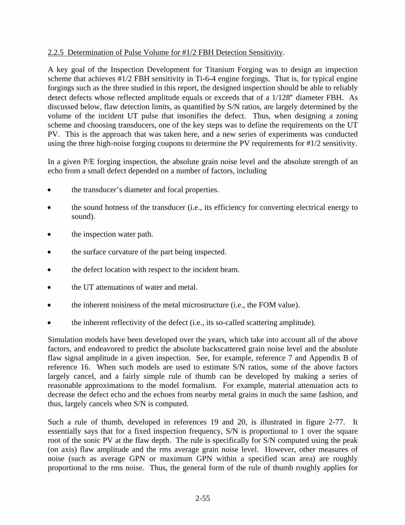
2-55

2.2.5 Determination of Pulse Volume for #1/2 FBH Detection Sensitivity.

A key goal of the Inspection Development for Titanium Forging was to design an inspection scheme that achieves #1/2 FBH sensitivity in Ti-6-4 engine forgings. That is, for typical engine forgings such as the three studied in this report, the designed inspection should be able to reliably detect defects whose reflected amplitude equals or exceeds that of a 1/128″ diameter FBH. As discussed below, flaw detection limits, as quantified by S/N ratios, are largely determined by the volume of the incident UT pulse that insonifies the defect. Thus, when designing a zoning scheme and choosing transducers, one of the key steps was to define the requirements on the UT PV. This is the approach that was taken here, and a new series of experiments was conducted using the three high-noise forging coupons to determine the PV requirements for #1/2 sensitivity. In a given P/E forging inspection, the absolute grain noise level and the absolute strength of an echo from a small defect depended on a number of factors, including • the transducer’s diameter and focal properties.

• the sound hotness of the transducer (i.e., its efficiency for converting electrical energy to sound).

• the inspection water path.

• the surface curvature of the part being inspected.

• the defect location with respect to the incident beam.

• the UT attenuations of water and metal.

• the inherent noisiness of the metal microstructure (i.e., the FOM value).

• the inherent reflectivity of the defect (i.e., its so-called scattering amplitude).

Simulation models have been developed over the years, which take into account all of the above factors, and endeavored to predict the absolute backscattered grain noise level and the absolute flaw signal amplitude in a given inspection. See, for example, reference 7 and Appendix B of reference 16. When such models are used to estimate S/N ratios, some of the above factors largely cancel, and a fairly simple rule of thumb can be developed by making a series of reasonable approximations to the model formalism. For example, material attenuation acts to decrease the defect echo and the echoes from nearby metal grains in much the same fashion, and thus, largely cancels when S/N is computed. Such a rule of thumb, developed in references 19 and 20, is illustrated in figure 2-77. It essentially says that for a fixed inspection frequency, S/N is proportional to 1 over the square root of the sonic PV at the flaw depth. The rule is specifically for S/N computed using the peak (on axis) flaw amplitude and the rms average grain noise level. However, other measures of noise (such as average GPN or maximum GPN within a specified scan area) are roughly proportional to the rms noise. Thus, the general form of the rule of thumb roughly applies for

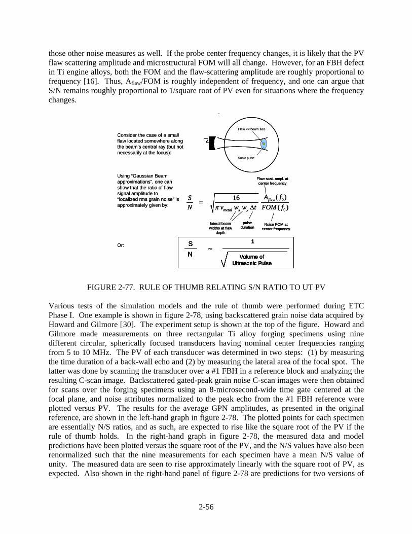
2-56

those other noise measures as well. If the probe center frequency changes, it is likely that the PV flaw scattering amplitude and microstructural FOM will all change. However, for an FBH defect in Ti engine alloys, both the FOM and the flaw-scattering amplitude are roughly proportional to frequency [16]. Thus, Aflaw/FOM is roughly independent of frequency, and one can argue that S/N remains roughly proportional to 1/square root of PV even for situations where the frequency changes. g

Flaw << beam size

Consider the case of a small flaw located somewhere along the beam’s central ray (but not necessarily at the focus):

Using “Gaussian Beam approximations”, one can show that the ratio of flaw signal amplitude to “localized rms grain noise” is approximately given by:

0

0

( )16( )

flaw

metal x y

A fSN v w w t FOM fπ

=Δ

pulseduration

lateral beamwidths at flaw

depth

Noise FOM at center frequency

Flaw scat. ampl. at center frequency

Sonic pulse

Or: SN Volume of

Ultrasonic Pulse

~1S

N Volume ofUltrasonic Pulse

Volume ofUltrasonic Pulse

~1

g

Flaw << beam size

Consider the case of a small flaw located somewhere along the beam’s central ray (but not necessarily at the focus):

Using “Gaussian Beam approximations”, one can show that the ratio of flaw signal amplitude to “localized rms grain noise” is approximately given by:

0

0

( )16( )

flaw

metal x y

A fSN v w w t FOM fπ

=Δ

pulseduration

lateral beamwidths at flaw

depth

Noise FOM at center frequency

Flaw scat. ampl. at center frequency

0

0

( )16( )

flaw

metal x y

A fSN v w w t FOM fπ

=Δ

pulseduration

lateral beamwidths at flaw

depth

Noise FOM at center frequency

Flaw scat. ampl. at center frequency

Sonic pulse

Or: SN Volume of

Ultrasonic Pulse

~1S

N Volume ofUltrasonic Pulse

Volume ofUltrasonic Pulse

~1S

N Volume ofUltrasonic Pulse

~1S

N Volume ofUltrasonic Pulse

Volume ofUltrasonic Pulse

~1

FIGURE 2-77. RULE OF THUMB RELATING S/N RATIO TO UT PV Various tests of the simulation models and the rule of thumb were performed during ETC Phase I. One example is shown in figure 2-78, using backscattered grain noise data acquired by Howard and Gilmore [30]. The experiment setup is shown at the top of the figure. Howard and Gilmore made measurements on three rectangular Ti alloy forging specimens using nine different circular, spherically focused transducers having nominal center frequencies ranging from 5 to 10 MHz. The PV of each transducer was determined in two steps: (1) by measuring the time duration of a back-wall echo and (2) by measuring the lateral area of the focal spot. The latter was done by scanning the transducer over a #1 FBH in a reference block and analyzing the resulting C-scan image. Backscattered gated-peak grain noise C-scan images were then obtained for scans over the forging specimens using an 8-microsecond-wide time gate centered at the focal plane, and noise attributes normalized to the peak echo from the #1 FBH reference were plotted versus PV. The results for the average GPN amplitudes, as presented in the original reference, are shown in the left-hand graph in figure 2-78. The plotted points for each specimen are essentially N/S ratios, and as such, are expected to rise like the square root of the PV if the rule of thumb holds. In the right-hand graph in figure 2-78, the measured data and model predictions have been plotted versus the square root of the PV, and the N/S values have also been renormalized such that the nine measurements for each specimen have a mean N/S value of unity. The measured data are seen to rise approximately linearly with the square root of PV, as expected. Also shown in the right-hand panel of figure 2-78 are predictions for two versions of

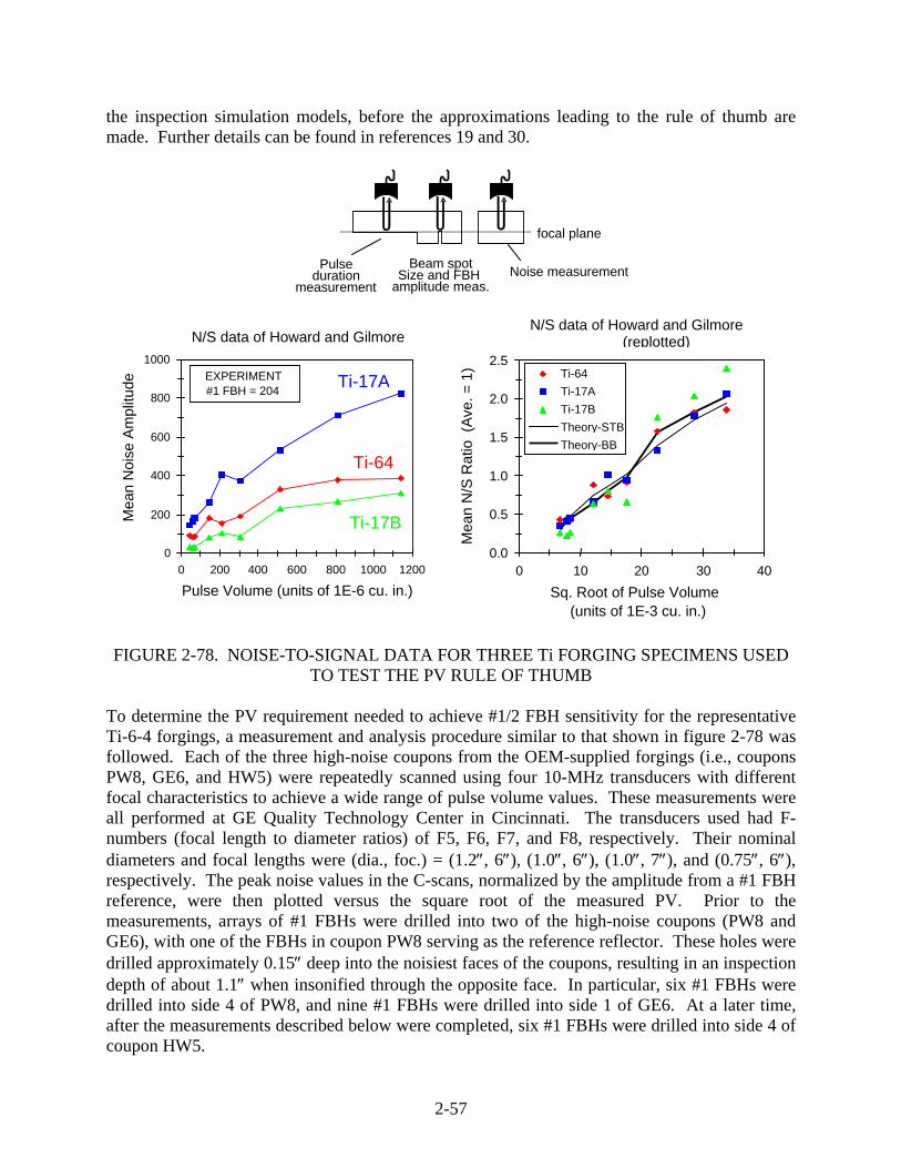
2-57

the inspection simulation models, before the approximations leading to the rule of thumb are made. Further details can be found in references 19 and 30.

FIGURE 2-78. NOISE-TO-SIGNAL DATA FOR THREE Ti FORGING SPECIMENS USED

TO TEST THE PV RULE OF THUMB To determine the PV requirement needed to achieve #1/2 FBH sensitivity for the representative Ti-6-4 forgings, a measurement and analysis procedure similar to that shown in figure 2-78 was followed. Each of the three high-noise coupons from the OEM-supplied forgings (i.e., coupons PW8, GE6, and HW5) were repeatedly scanned using four 10-MHz transducers with different focal characteristics to achieve a wide range of pulse volume values. These measurements were all performed at GE Quality Technology Center in Cincinnati. The transducers used had F-numbers (focal length to diameter ratios) of F5, F6, F7, and F8, respectively. Their nominal diameters and focal lengths were (dia., foc.) = (1.2″, 6″), (1.0″, 6″), (1.0″, 7″), and (0.75″, 6″), respectively. The peak noise values in the C-scans, normalized by the amplitude from a #1 FBH reference, were then plotted versus the square root of the measured PV. Prior to the measurements, arrays of #1 FBHs were drilled into two of the high-noise coupons (PW8 and GE6), with one of the FBHs in coupon PW8 serving as the reference reflector. These holes were drilled approximately 0.15″ deep into the noisiest faces of the coupons, resulting in an inspection depth of about 1.1″ when insonified through the opposite face. In particular, six #1 FBHs were drilled into side 4 of PW8, and nine #1 FBHs were drilled into side 1 of GE6. At a later time, after the measurements described below were completed, six #1 FBHs were drilled into side 4 of coupon HW5.

Pulse duration

measurement

Beam spotSize and FBH

amplitude meas.Noise measurement

focal plane

0

200

400

600

800

1000

0 200 400 600 800 1000 1200

Pulse Volume (units of 1E-6 cu. in.)

Mea

n N

oise

Am

plitu

de

Ti-17A

Ti-17B

Ti-64

EXPERIMENT #1 FBH = 204

N/S data of Howard and Gilmore

0.0

0.5

1.0

1.5

2.0

2.5

0 10 20 30 40Sq. Root of Pulse Volume

(units of 1E-3 cu. in.)

Mea

n N

/S R

atio

(A

ve. =

1) Ti-64

Ti-17ATi-17BTheory-STBTheory-BB

N/S data of Howard and Gilmore (replotted)

2-58

The C-scan data for one case is shown in figure 2-79. The transducer was the F6 probe, and the water path was chosen to focus the sound beam at the depth of the FBHs. The inspection gain was set such that the response from the #1 FBH reference hole would be at 320% FSH, or equivalent, and that the response from a #1/2 FBH would be approximately 80% FSH. The peak noise was measured for each of the high-noise coupons shown in the figure, resulting in 30.6%, 43.0%, and 36% FSH for the P&W, HW, and GE coupons respectively. The time gate used for all C-scan measurements was 1.6 microseconds wide (corresponding to about 0.2″ of metal depth), centered approximately at the FBH depth.

FIGURE 2-79. NOISE-TO-SIGNAL MEASUREMENTS FOR THE THREE HIGH-NOISE FORGING COUPONS

In addition to the N/S measurements, sonic PVs were also measured. First, the -6dB beam diameter at the FBH depth was determined from a fine-increment C-scan of the reference hole in the PW8 coupon. Figure 2-80 shows the beam diameter determination for the F6 example, leading to a value of 39.4 mils. Second, as shown in figure 2-81, the pulse duration was measured by finding the -6 dB points for the envelope function of the rectified FBH echo, then it was translated to a pulse length in metal. For the case shown, the pulse length was 36.7 mils, leading to a measured PV of (π/4)(39.4 mils)2(36.7mils) = 44,600 cubic mils. Similar measurements of peak N/S amplitudes and sonic PVs were made for a total of nine configurations (transducer and water path combinations). For most transducers, measurements were made using more than one water path to vary the beam spot size at the FBH depth. For the F6 transducer, for example, three water paths were used: one chosen to maximize the amplitude from the reference FBH and two longer water paths for which the peak FBH amplitude was down by 3 and 6 dB, respectively, from the first case. Measured N/S amplitudes and sonic PVs

#1/2 FBH ~ 80%

HW5Max noise43%

GE6Max. noise36%

PW8Max. noise30.6%

2-59

for the nine measurement configurations are listed in table 2-4, and N/S is plotted versus the square root of PV, as shown in figure 2-82. For each coupon, the trend of the data approximately follows a straight line that passes through the origin, as expected from the rule of thumb. The slope of the line is different for each coupon; that slope is expected to be approximately proportional to the average FOM value within the time gate, although, strictly speaking, one would need to measure both the noise level and the FBH reference amplitude in the same specimen for this to be true. Coupon HW5 has the highest slope while the slopes for the PW8 and GE6 coupons are similar. This ordering is in good agreement with the ordering of peak FOM curves near 10 MHz for these three coupons.

FIGURE 2-80. BEAM DIAMETER DETERMINATION FOR THE 10-MHz F6 TRANSDUCER FOCUSED AT THE FBH DEPTH

FIGURE 2-81. PULSE DURATION DETERMINATION FOR THE

10-MHz F6 TRANSDUCER FOCUSED AT THE FBH DEPTH

FBH C-scan

All pixels with amplitudes within 6 dB of the maximum are located, and their joint area is measured.FBH C-scan

All pixels with amplitudes within 6 dB of the maximum are located, and their joint area is measured.

Microseconds

0

25

50

75

100

125

0.0 0.1 0.2 0.3 0.4 0.5 0.6 0.7

Am

plitu

de The full width of the

envelope of the rectified FBH echo at the –6 dB level (50% of the maximum) is 0.150 microseconds.

F6-0dB-Rect

F6-0dB-Env

2-60

TABLE 2-4. MEASURED SONIC PV AND PEAK N/S RATIOS FOR THE HIGHEST-NOISE COUPONS FROM THE THREE OEM-SUPPLIED Ti-6-4 FORGINGS

Peak N/S Ratio Transducer Location

PV (cubic mils)

PV (Sqrt) PW8 HW5 GE6

F5 0 dB 20173 142.0324 25.0 29.0 25.0 F5 -3 dB 26633 163.1952 29.8 41.5 31.3 F5 -6 dB 34972 187.0091 39.0 50.9 39.2 F6 0 dB 44613 211.2176 30.6 43.0 36.0 F6 -3 dB 57029 238.8072 38.4 58.8 47.0 F6 -6 dB 69354 263.3516 42.7 66.3 54.9 F7 0 dB 51013 225.8606 40.8 43.9 37.6 F7 -3 dB 68170 261.0929 48.0 67.5 52.5 F8 0 dB 79673 282.2649 53.0 74.5 50.0

FIGURE 2-82. PEAK N/S VS THE SQUARE ROOT OF PV FOR MEASUREMENTS PERFORMED ON THE HIGHEST-NOISE COUPONS

CUT FROM THE THREE OEM-SUPPLIED Ti-6-4 FORGINGS As discussed in the ETC Phase II final report for the Forging Inspection Development subtask [31], a goal was set to develop and demonstrate #1/2 FBH detection sensitivity for zoned inspections of Ti-6-4 forgings. This was specifically taken to mean that within each inspection zone, the peak noise anywhere within a C-scan image should be at least 3 dB below the response from a #1/2 FBH located in that zone. The target inspection sensitivity is indicated by the magenta line in figure 2-82, which at 56.6% FSH, is 3 dB below the amplitude from a #1/2 reference hole (80% FSH on the same scale). From the measurements one can conclude that

0.0

10.0

20.0

30.0

40.0

50.0

60.0

70.0

80.0

0 100 200 300

Sqrt (Pulse Volume in cubic mils)

Peak

-Noi

se-t

o-Si

gnal

(% F

SH)

PW8HW5GE6

#1 FBH at 12 dB above 80%or at 318.5% on this scale

F6 @

-3dB

F5 @

-3dB

56.6% (3 dB below 80%)

F6 @

0dB

For each specimen,Rule-of-Thumb wouldpredict a straight linepassing thru origin.Slope dependent on FOM

F5 @

0dB F8

@ 0

dB

1.6 usec time gate

#1/2 FBHapprox at 80%on this scale.

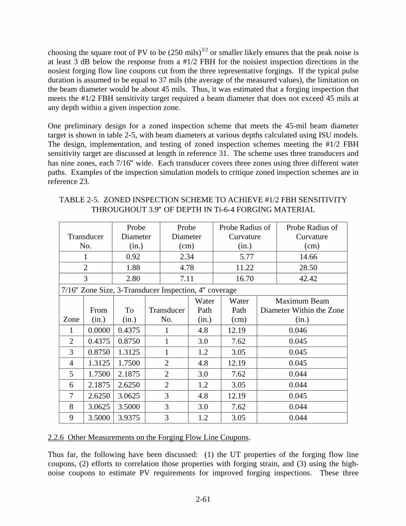
2-61

choosing the square root of PV to be (250 mils)3/2 or smaller likely ensures that the peak noise is at least 3 dB below the response from a #1/2 FBH for the noisiest inspection directions in the nosiest forging flow line coupons cut from the three representative forgings. If the typical pulse duration is assumed to be equal to 37 mils (the average of the measured values), the limitation on the beam diameter would be about 45 mils. Thus, it was estimated that a forging inspection that meets the #1/2 FBH sensitivity target required a beam diameter that does not exceed 45 mils at any depth within a given inspection zone. One preliminary design for a zoned inspection scheme that meets the 45-mil beam diameter target is shown in table 2-5, with beam diameters at various depths calculated using ISU models. The design, implementation, and testing of zoned inspection schemes meeting the #1/2 FBH sensitivity target are discussed at length in reference 31. The scheme uses three transducers and has nine zones, each 7/16″ wide. Each transducer covers three zones using three different water paths. Examples of the inspection simulation models to critique zoned inspection schemes are in reference 23.

TABLE 2-5. ZONED INSPECTION SCHEME TO ACHIEVE #1/2 FBH SENSITIVITY THROUGHOUT 3.9″ OF DEPTH IN Ti-6-4 FORGING MATERIAL

Transducer No.

Probe Diameter

(in.)

Probe Diameter

(cm)

Probe Radius of Curvature

(in.)

Probe Radius of Curvature

(cm) 1 0.92 2.34 5.77 14.66 2 1.88 4.78 11.22 28.50 3 2.80 7.11 16.70 42.42

7/16″ Zone Size, 3-Transducer Inspection, 4″ coverage

Zone From (in.)

To (in.)

Transducer No.

Water Path (in.)

Water Path (cm)

Maximum Beam Diameter Within the Zone

(in.) 1 0.0000 0.4375 1 4.8 12.19 0.046 2 0.4375 0.8750 1 3.0 7.62 0.045 3 0.8750 1.3125 1 1.2 3.05 0.045 4 1.3125 1.7500 2 4.8 12.19 0.045 5 1.7500 2.1875 2 3.0 7.62 0.044 6 2.1875 2.6250 2 1.2 3.05 0.044 7 2.6250 3.0625 3 4.8 12.19 0.045 8 3.0625 3.5000 3 3.0 7.62 0.044 9 3.5000 3.9375 3 1.2 3.05 0.044

2.2.6 Other Measurements on the Forging Flow Line Coupons.

Thus far, the following have been discussed: (1) the UT properties of the forging flow line coupons, (2) efforts to correlation those properties with forging strain, and (3) using the high-noise coupons to estimate PV requirements for improved forging inspections. These three

2-62

studies largely fulfilled the intended uses for these coupons. However, a few other inquires were pursued using the forging flow line coupons, which are also worthy of mention. 2.2.6.1 Additional Measurements on the P&W Forging Coupons.

In addition to the systematic UT property measurements performed at ISU on coupons from all three forgings, some OEMs performed independent measurements on the coupons taken from their own forgings. The most complete study was conducted by P&W personnel who measured velocity, attenuation, and backscattered noise in three different inspection directions for each of the seven rectangular P&W coupons. The enumeration scheme they used for the radial, axial, and circumferential faces of the coupons is shown in figure 2-83. Note that it differs from the ISU measurements (figure 2-39).

up

hub

1 (circumferential)

2 (radial)

3 (axial)

1

2

3 4

5

6

6

1

2

3

4

5

1 2

3 4up

hub

up

hub

1 (circumferential)

2 (radial)

3 (axial)

1

2

3 4

5

6

6

1

2

3

4

5

1 2

3 4

FIGURE 2-83. INSPECTION DIRECTION LABELS FOR MEASUREMENTS

BY P&W PERSONNEL (With velocity measurement positions indicated.)

Longitudinal-wave velocities were deduced from measurements of the time delays between the first and second back-wall echoes using a 10-MHz, 3/8″ diameter planar probe in immersion. For the radial and axial directions, the velocity was measured at six positions, as indicated in figure 2-83, and the results were averaged. In the circumferential direction, the velocity was measured at four positions. Measured velocities in the radial, hoop, and axial directions are shown in figure 2-84 for the seven P&W coupons. Both the average values (plotted points) and standard deviations (vertical bars) of the measurements are indicated for each inspection direction. The variability in the velocity throughout the suite of coupons was quite small, ranging from a low of 6.19 mm/μsec to a high of 6.24 mm/μsec, a range of about 0.8%. In the axial direction (i.e., the typical inspection direction), a clear trend was observed, with the velocity increasing by about 0.4% from the bore towards the rim. This same trend was observed in the ISU measurements (figure 2-49).

2-63

1

2

3

4

5

6

7

8Radial (2)

Axial (3)

Circumferential (1)

6.180

6.190

6.200

6.210

6.220

6.230

6.240

6.250

0 2 4 6 8 10

Test block

Velo

city

, mm

/ μs

radialhoopnormal

0.4%

FIGURE 2-84. LONGITUDINAL VELOCITIES FOR THE SEVEN RECTANGULAR P&W FORGING FLOW LINE COUPONS

Attenuation measurements performed by P&W personnel followed the general procedure developed at the ISU. The first back-wall reflection at a given point in the forging coupon was compared to the back-wall reflection from a low-attenuation block of similar thickness, in this case, a block of fine-grained Ni alloy IN1100. By comparing the spectra of the two back-wall echoes, the attenuation-versus-frequency curve for the metal specimen can be deduced within the bandwidth of the transducer [18]. For measurements on the seven rectangular coupons from the P&W forging, the 10-MHz, 3/8″ diameter planar transducer was again used. For each inspection direction, attenuation curves were deduced at approximately 100 points by scanning the transducer over the central region of the entry surface. For measurements in the axial and radial directions, the scan area was 0.8″ by 1.2″. For measurements in the circumferential direction, the scan area was 0.5″ by 0.5″. As is generally the case for engine Ti specimens, for a fixed inspection direction, substantial variations were observed in the strength of the back-wall echo from position-to-position within a given coupon. For a given inspection direction, the attenuation-versus-frequency curves measured at the various scan locations were averaged, and the average curve was fit to a power law of the form Attenuation (N/cm) = (A)(Frequency in MHz)

1.5 (2-1)

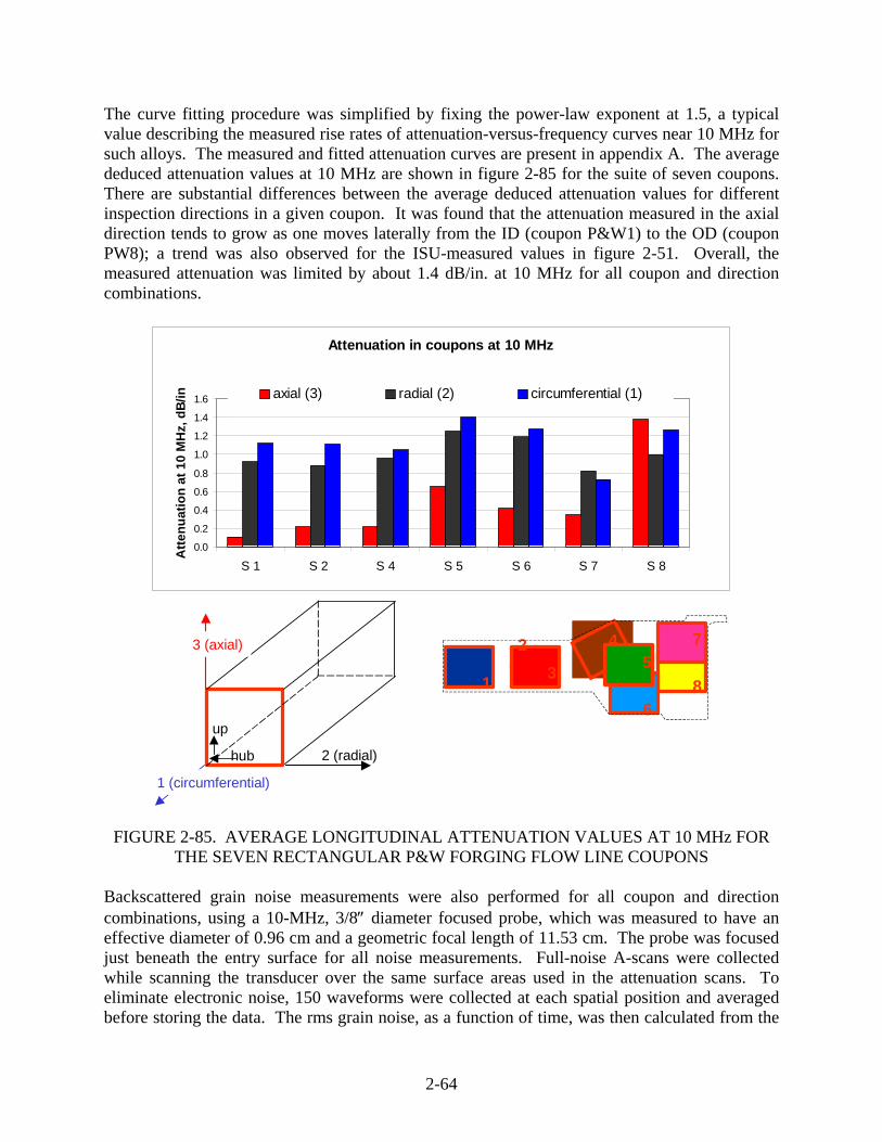
2-64

The curve fitting procedure was simplified by fixing the power-law exponent at 1.5, a typical value describing the measured rise rates of attenuation-versus-frequency curves near 10 MHz for such alloys. The measured and fitted attenuation curves are present in appendix A. The average deduced attenuation values at 10 MHz are shown in figure 2-85 for the suite of seven coupons. There are substantial differences between the average deduced attenuation values for different inspection directions in a given coupon. It was found that the attenuation measured in the axial direction tends to grow as one moves laterally from the ID (coupon P&W1) to the OD (coupon PW8); a trend was also observed for the ISU-measured values in figure 2-51. Overall, the measured attenuation was limited by about 1.4 dB/in. at 10 MHz for all coupon and direction combinations.

1

23

45

6

7

8

up

hub 2 (radial)

3 (axial)

Attenuation in coupons at 10 MHz

0.0

0.2

0.4

0.6

0.8

1.0

1.2

1.4

1.6

S 1 S 2 S 4 S 5 S 6 S 7 S 8

Atte

nuat

ion

at 1

0 M

Hz,

dB/

in axial (3) radial (2) circumferential (1)

1 (circumferential)

FIGURE 2-85. AVERAGE LONGITUDINAL ATTENUATION VALUES AT 10 MHz FOR

THE SEVEN RECTANGULAR P&W FORGING FLOW LINE COUPONS Backscattered grain noise measurements were also performed for all coupon and direction combinations, using a 10-MHz, 3/8″ diameter focused probe, which was measured to have an effective diameter of 0.96 cm and a geometric focal length of 11.53 cm. The probe was focused just beneath the entry surface for all noise measurements. Full-noise A-scans were collected while scanning the transducer over the same surface areas used in the attenuation scans. To eliminate electronic noise, 150 waveforms were collected at each spatial position and averaged before storing the data. The rms grain noise, as a function of time, was then calculated from the

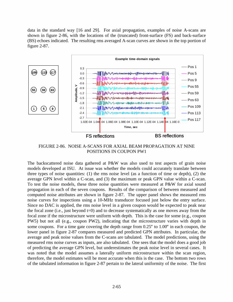
2-65

data in the standard way [16 and 29]. For axial propagation, examples of noise A-scans are shown in figure 2-86, with the locations of the (truncated) front-surface (FS) and back-surface (BS) echoes indicated. The resulting rms averaged A-scan curves are shown in the top portion of figure 2-87.

Example time-domain signals

-2.7

-2.4

-2.1

-1.8

-1.5

-1.2

-0.9

-0.6

-0.3

0.0

0.3

1.02E-04 1.04E-04 1.06E-04 1.08E-04 1.10E-04 1.12E-04 1.14E-04 1.16E-04

Time, sec

Am

plitu

de, V

Pos 1

Pos 5

Pos 9

Pos 55

Pos 59

Pos 63

Pos 109

Pos 113

Pos 117

51 9

5955 63

113109 117

FS reflections BS reflections

Example time-domain signals

-2.7

-2.4

-2.1

-1.8

-1.5

-1.2

-0.9

-0.6

-0.3

0.0

0.3

1.02E-04 1.04E-04 1.06E-04 1.08E-04 1.10E-04 1.12E-04 1.14E-04 1.16E-04

Time, sec

Am

plitu

de, V

Pos 1

Pos 5

Pos 9

Pos 55

Pos 59

Pos 63

Pos 109

Pos 113

Pos 117

51 9

5955 63

113109 117

51 9

5955 63

113109 117

FS reflections BS reflections

FIGURE 2-86. NOISE A-SCANS FOR AXIAL BEAM PROPAGATION AT NINE POSITIONS IN COUPON PW1

The backscattered noise data gathered at P&W was also used to test aspects of grain noise models developed at ISU. At issue was whether the models could accurately translate between three types of noise quantities: (1) the rms noise level (as a function of time or depth), (2) the average GPN level within a C-scan, and (3) the maximum or peak GPN value within a C-scan. To test the noise models, these three noise quantities were measured at P&W for axial sound propagation in each of the seven coupons. Results of the comparison of between measured and computed noise attributes are shown in figure 2-87. The upper panel shows the measured rms noise curves for inspections using a 10-MHz transducer focused just below the entry surface. Since no DAC is applied, the rms noise level in a given coupon would be expected to peak near the focal zone (i.e., just beyond t=0) and to decrease systematically as one moves away from the focal zone if the microstructure were uniform with depth. This is the case for some (e.g., coupon PW5) but not all (e.g., coupon PW2), indicating that the microstructure varies with depth in some coupons. For a time gate covering the depth range from 0.25″ to 1.00″ in each coupon, the lower panel in figure 2-87 compares measured and predicted GPN attributes. In particular, the average and peak noise values from the C-scans are tabulated. The model predictions, using the measured rms noise curves as inputs, are also tabulated. One sees that the model does a good job of predicting the average GPN level, but underestimates the peak noise level in several cases. It was noted that the model assumes a laterally uniform microstructure within the scan region, therefore, the model estimates will be most accurate when this is the case. The bottom two rows of the tabulated information in figure 2-87 pertain to the lateral uniformity of the noise. The first

2-66

(a)

Coupon 1 Coupon 2 Coupon 4 Coupon 5 Coupon 6 Coupon 7 Coupon 8

Experimental summary. Time gate for C-scan extends from 0.25″-1.00″. All noise values are in Volts at fixed gain. Max. rms value in gate 0.0374 0.0370 0.0233 0.0371 0.0323 0.0405 0.0259

Max. gated peak noise 0.1302 0.1606 0.0777 0.1454 0.2184 0.2343 0.1321

Average gated peak noise 0.1044 0.1071 0.053 0.0892 0.0727 0.0952 0.0616

Averages

Ratio max. gated peak/rms 3.48 4.34 3.34 3.92 6.76 5.79 5.09 4.7

Ratio avg. gated peak/rms 2.79 2.89 2.28 2.40 2.25 2.35 2.38 2.5

Theory predictions, using the rms_noise_vs_time curve on 0.25″-1.00″ as input. 117 probe positions in scan. Max. rms value in gate 0.0374 0.0370 0.0233 0.0371 0.0323 0.0405 0.0259

Max. gated peak noise 0.1476 0.1499 0.084 0.1361 0.1181 0.1483 0.0938

Average gated peak noise 0.099792 0.101675 0.050877 0.084498 0.070964 0.091534 0.058439

Averages

Ratio max. gated peak/rms 3.94 4.05 3.61 3.67 3.66 3.66 3.62 3.7

Ratio avg. gated peak/rms 2.67 2.75 2.18 2.28 2.20 2.26 2.25 2.4

Comment on lateral uniformity

of noise within coupon: Average Good Very Good Average Average Very Bad Bad

Std,/Dev,/mean for ISU 0.246 0.228 0.197 0.260 0.247 0.387 0.310

Gated-peak noise meas.

(b)

FIGURE 2-87. (a) MEASURED RMS NOISE CURVES, AS FUNCTIONS OF TIME RELATIVE TO THE FRONT-WALL ECHO (t=0), FOR THE SEVEN RECTANGULAR

P&W FORGING COUPONS AND (b) TABULAR COMPARISONS OF MEASURED AND PREDICTED GPN QUANTITIES

0.010

0.015

0.020

0.025

0.030

0.035

0.040

0.045

0.050

0 2 4 6 8 10

Time after FS echo (μsec)

RM

S no

ise

(Vol

ts)

Coupon 1

Coupon 2

Coupon 4

Coupon 5

Coupon 6

Coupon 7

Coupon 8

Time gate -scans –1.00Time gate for C-scans (0.25″-1.00″)

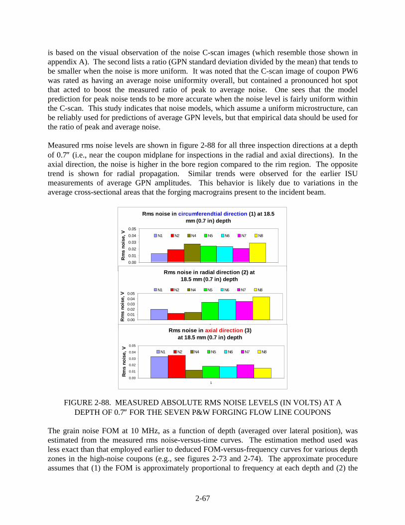
2-67

is based on the visual observation of the noise C-scan images (which resemble those shown in appendix A). The second lists a ratio (GPN standard deviation divided by the mean) that tends to be smaller when the noise is more uniform. It was noted that the C-scan image of coupon PW6 was rated as having an average noise uniformity overall, but contained a pronounced hot spot that acted to boost the measured ratio of peak to average noise. One sees that the model prediction for peak noise tends to be more accurate when the noise level is fairly uniform within the C-scan. This study indicates that noise models, which assume a uniform microstructure, can be reliably used for predictions of average GPN levels, but that empirical data should be used for the ratio of peak and average noise. Measured rms noise levels are shown in figure 2-88 for all three inspection directions at a depth of 0.7″ (i.e., near the coupon midplane for inspections in the radial and axial directions). In the axial direction, the noise is higher in the bore region compared to the rim region. The opposite trend is shown for radial propagation. Similar trends were observed for the earlier ISU measurements of average GPN amplitudes. This behavior is likely due to variations in the average cross-sectional areas that the forging macrograins present to the incident beam.

FIGURE 2-88. MEASURED ABSOLUTE RMS NOISE LEVELS (IN VOLTS) AT A DEPTH OF 0.7″ FOR THE SEVEN P&W FORGING FLOW LINE COUPONS

The grain noise FOM at 10 MHz, as a function of depth (averaged over lateral position), was estimated from the measured rms noise-versus-time curves. The estimation method used was less exact than that employed earlier to deduced FOM-versus-frequency curves for various depth zones in the high-noise coupons (e.g., see figures 2-73 and 2-74). The approximate procedure assumes that (1) the FOM is approximately proportional to frequency at each depth and (2) the

Rms noise in circumferendtial direction (1) at 18.5 mm (0.7 in) depth

0.000.010.020.030.040.05

1

Rm

s no

ise,

V N1 N2 N4 N5 N6 N7 N8

Rms noise in radial direction (2) at 18.5 mm (0.7 in) depth

0.000.010.020.030.040.05

1

Rm

s no

ise,

V

N1 N2 N4 N5 N6 N7 N8

Rms noise in axial direction (3) at 18.5 mm (0.7 in) depth

0.00

0.01

0.02

0.03

0.04

0.05

1

Rms

nois

e, V N1 N2 N4 N5 N6 N7 N8

2-68

measured rms noise level at a given depth is directly proportional to the local FOM value (evaluated at the center frequency) at that depth. This approximate FOM estimation method is discussed in more detail in reference 32. The deduced FOM-versus-depth curves obtained in this manner may be found in appendix A. The FOM values at 10 MHz were found to be limited by 0.025 1/cm1/2 in all cases and showed the same general behavior on inspection direction and coupon location as the rms noise values in figure 2-88. For axial beam propagation, figure 2-89 compares the measured attenuation values with the measured FOM values near the coupon midplanes. One sees a clear inverse relationship between attenuation and noise attributes. This is reminiscent of the inverse correlation between attenuation and noise anisotropy in coupons from all three forgings in the ISU study (figure 2-67).

FIGURE 2-89. MEASURED ATTENUATION AND FOM VALUES FOR AXIAL BEAM PROPAGATION IN THE SEVEN P&W FORGING FLOW LINE COUPONS

In general, the UT property measurements performed by P&W personnel were found to be in good agreement with those reported by ISU researchers, when comparing the graphs in this section (and in appendix A) with those presented in figures 2-45, 2-49, and 2-51. Since different approaches were taken in the measurement of grain noise attributes, not all of the measured values could be directly compared. However, when direct comparison was not possible, quantities that were expected to be nearly proportional to one another were found to be so. An example is shown in figure 2-90 where two measures of backscattered grain noise levels in the P&W forging flow line coupons are compared. The vertical axis displays the noise FOM at 10 MHz and a depth of 0.31″, as estimated by P&W personnel using a 10-MHz focused probe. The horizontal axis displays the measured average GPN level, relative to a #1 FBH, as measured at ISU using a 15-MHz probe focused approximately 0.31″ deep. Each plotted point represents one coupon inspected from one direction, with values averaged over the lateral area of the entry

Attenuation in axial (3) direction at 10 MHz

0.0

0.2

0.4

0.6

0.8

1.0

1.2

1.4

1.6

1.8

1Samples

Atte

nuat

ion,

dB

/in

S 1 S 2 S 4 S 5 S 6 S 7 S 8

Axial (3) direction: FOM at 10 MHz at 2 cm depth

0.000

0.005

0.010

0.015

0.020

0.025

0.030

1

FOM-1 FOM-2 FOM-4 FOM-5 FOM-6 FOM-7 FOM-8

radial

axial

circumferential1

2

3

4

5

6

7

8

Attenuation in axial (3) direction at 10 MHz

0.0

0.2

0.4

0.6

0.8

1.0

1.2

1.4

1.6

1.8

1Samples

Atte

nuat

ion,

dB

/in

S 1 S 2 S 4 S 5 S 6 S 7 S 8

Axial (3) direction: FOM at 10 MHz at 2 cm depth

0.000

0.005

0.010

0.015

0.020

0.025

0.030

1

FOM-1 FOM-2 FOM-4 FOM-5 FOM-6 FOM-7 FOM-8

radial

axial

circumferential

radial

axial

circumferential1

2

3

4

5

6

7

81

2

3

4

5

6

7

8

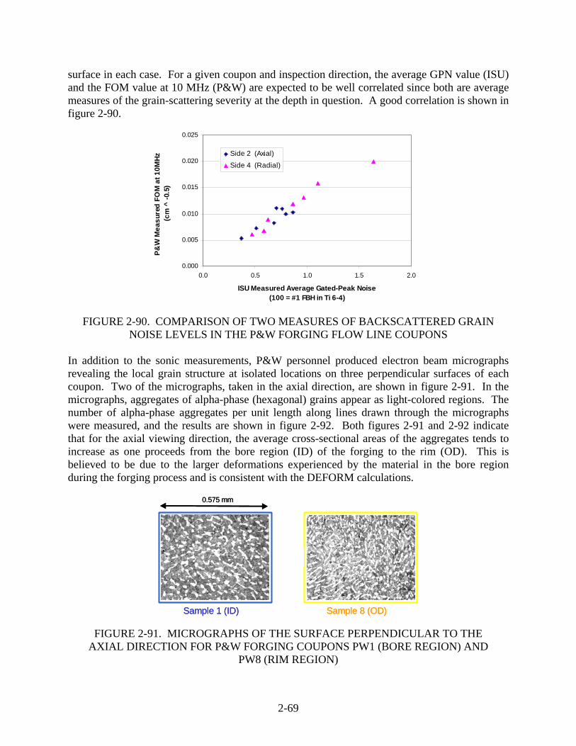
2-69

surface in each case. For a given coupon and inspection direction, the average GPN value (ISU) and the FOM value at 10 MHz (P&W) are expected to be well correlated since both are average measures of the grain-scattering severity at the depth in question. A good correlation is shown in figure 2-90.

FIGURE 2-90. COMPARISON OF TWO MEASURES OF BACKSCATTERED GRAIN NOISE LEVELS IN THE P&W FORGING FLOW LINE COUPONS

In addition to the sonic measurements, P&W personnel produced electron beam micrographs revealing the local grain structure at isolated locations on three perpendicular surfaces of each coupon. Two of the micrographs, taken in the axial direction, are shown in figure 2-91. In the micrographs, aggregates of alpha-phase (hexagonal) grains appear as light-colored regions. The number of alpha-phase aggregates per unit length along lines drawn through the micrographs were measured, and the results are shown in figure 2-92. Both figures 2-91 and 2-92 indicate that for the axial viewing direction, the average cross-sectional areas of the aggregates tends to increase as one proceeds from the bore region (ID) of the forging to the rim (OD). This is believed to be due to the larger deformations experienced by the material in the bore region during the forging process and is consistent with the DEFORM calculations.

FIGURE 2-91. MICROGRAPHS OF THE SURFACE PERPENDICULAR TO THE AXIAL DIRECTION FOR P&W FORGING COUPONS PW1 (BORE REGION) AND

PW8 (RIM REGION)

0.000

0.005

0.010

0.015

0.020

0.025

0.0 0.5 1.0 1.5 2.0

ISU Measured Average Gated-Peak Noise(100 = #1 FBH in Ti 6-4)

P&W

Mea

sure

d FO

M a

t 10M

Hz (c

m ^

-0.5

)

Side 2 (Axial)Side 4 (Radial)

Sample 1 (ID) Sample 8 (OD)

0.575 mm

Sample 1 (ID) Sample 8 (OD)

0.575 mm

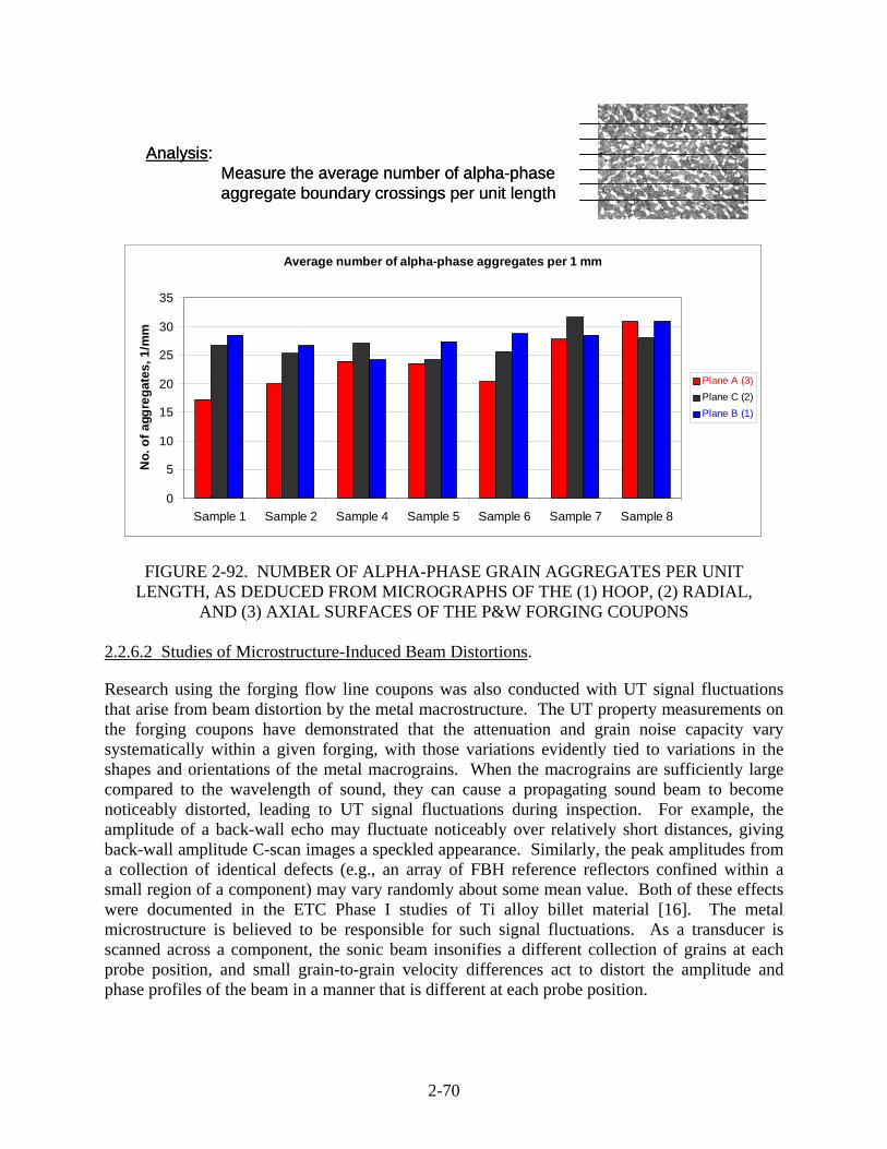
2-70

Average number of alpha-phase aggregates per 1 mm

0

5

10

15

20

25

30

35

Sample 1 Sample 2 Sample 4 Sample 5 Sample 6 Sample 7 Sample 8

No.

of a

ggre

gate

s, 1

/mm

Plane A (3)Plane C (2)Plane B (1)

Analysis: Measure the average number of alpha-phaseaggregate boundary crossings per unit length

Average number of alpha-phase aggregates per 1 mm

0

5

10

15

20

25

30

35

Sample 1 Sample 2 Sample 4 Sample 5 Sample 6 Sample 7 Sample 8

No.

of a

ggre

gate

s, 1

/mm

Plane A (3)Plane C (2)Plane B (1)

Analysis: Measure the average number of alpha-phaseaggregate boundary crossings per unit length

FIGURE 2-92. NUMBER OF ALPHA-PHASE GRAIN AGGREGATES PER UNIT LENGTH, AS DEDUCED FROM MICROGRAPHS OF THE (1) HOOP, (2) RADIAL,

AND (3) AXIAL SURFACES OF THE P&W FORGING COUPONS 2.2.6.2 Studies of Microstructure-Induced Beam Distortions.

Research using the forging flow line coupons was also conducted with UT signal fluctuations that arise from beam distortion by the metal macrostructure. The UT property measurements on the forging coupons have demonstrated that the attenuation and grain noise capacity vary systematically within a given forging, with those variations evidently tied to variations in the shapes and orientations of the metal macrograins. When the macrograins are sufficiently large compared to the wavelength of sound, they can cause a propagating sound beam to become noticeably distorted, leading to UT signal fluctuations during inspection. For example, the amplitude of a back-wall echo may fluctuate noticeably over relatively short distances, giving back-wall amplitude C-scan images a speckled appearance. Similarly, the peak amplitudes from a collection of identical defects (e.g., an array of FBH reference reflectors confined within a small region of a component) may vary randomly about some mean value. Both of these effects were documented in the ETC Phase I studies of Ti alloy billet material [16]. The metal microstructure is believed to be responsible for such signal fluctuations. As a transducer is scanned across a component, the sonic beam insonifies a different collection of grains at each probe position, and small grain-to-grain velocity differences act to distort the amplitude and phase profiles of the beam in a manner that is different at each probe position.

2-71

One effect of microstructure-induced beam distortions is to alter the apparent attenuation that is deduced using back-wall echoes, since the measured attenuation then has contributions both from energy loss (true attenuation) and beam distortion effects [16]. A series of experiments was performed at ISU to directly measure the energy-loss attenuation and to compare it to that deduced from back-wall echoes. Three of the 1.25″ by 1.25″ by 2.0″ Ti-6-4 forging flow line coupons were selected for use in these studies: GE4 (from the mid-thickness OD region of the GE forging), HW7 (from the forward ID region of the HW forging), and PW2 (from the web region of the P&W forging). Back-wall C-scan images of these three coupons through the radial (side 1) and axial (side 2) faces are shown in figure 2-93. A 1/4″ diameter, 10-MHz broadband planar transducer was used. Since all six back-wall images were acquired at the same gain setting and through the same nominal thickness (1.25″), gross attenuation differences can be readily discerned. For example, axial beam propagation through coupon HW7 leads to the lowest average back-wall amplitude, indicating the highest attenuation of the six. For HW7 and PW2, back-wall attenuation is larger for axial propagation than for radial propagation; for GE4, this order is reversed. These attenuation differences are believed to stem from microstructural differences between the coupons, principally the sizes and shapes of the macrograins and their orientations relative to the axial and radial directions in the forgings. Within each C-scan image, a sound beam entering through side 1 (side 2) propagates in the radial (axial) direction of the original forging. Distance scales are in inches, as shown in figure 2-93. Local amplitude variations are shown, which arise from local variations in the metal microstructure. These amplitude variations led to differences in the measured attenuation values at different scan points.

GE 4 side 2 HW7 side 2 PW2 side 2

GE 4 side 1 HW7 side 1 PW2 side 1

@ 15 dB(axial)

@ 15 dB(radial)

Low High

GE 4 side 2 HW7 side 2 PW2 side 2

GE 4 side 1 HW7 side 1 PW2 side 1

@ 15 dB(axial)

@ 15 dB(radial)

Low HighLow High

FIGURE 2-93. BACK-WALL AMPLITUDE C-SCANS OF THREE Ti-6-4 FORGING FLOW LINE COUPONS ACQUIRED USING A 10-MHz PLANAR TRANSDUCER

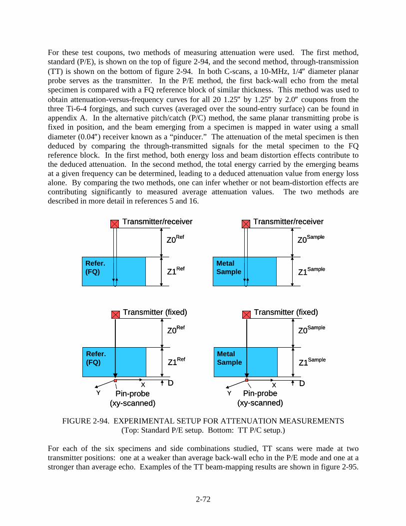
2-72

For these test coupons, two methods of measuring attenuation were used. The first method, standard (P/E), is shown on the top of figure 2-94, and the second method, through-transmission (TT) is shown on the bottom of figure 2-94. In both C-scans, a 10-MHz, 1/4″ diameter planar probe serves as the transmitter. In the P/E method, the first back-wall echo from the metal specimen is compared with a FQ reference block of similar thickness. This method was used to obtain attenuation-versus-frequency curves for all 20 1.25″ by 1.25″ by 2.0″ coupons from the three Ti-6-4 forgings, and such curves (averaged over the sound-entry surface) can be found in appendix A. In the alternative pitch/catch (P/C) method, the same planar transmitting probe is fixed in position, and the beam emerging from a specimen is mapped in water using a small diameter (0.04″) receiver known as a “pinducer.” The attenuation of the metal specimen is then deduced by comparing the through-transmitted signals for the metal specimen to the FQ reference block. In the first method, both energy loss and beam distortion effects contribute to the deduced attenuation. In the second method, the total energy carried by the emerging beams at a given frequency can be determined, leading to a deduced attenuation value from energy loss alone. By comparing the two methods, one can infer whether or not beam-distortion effects are contributing significantly to measured average attenuation values. The two methods are described in more detail in references 5 and 16.

FIGURE 2-94. EXPERIMENTAL SETUP FOR ATTENUATION MEASUREMENTS (Top: Standard P/E setup. Bottom: TT P/C setup.)

For each of the six specimens and side combinations studied, TT scans were made at two transmitter positions: one at a weaker than average back-wall echo in the P/E mode and one at a stronger than average echo. Examples of the TT beam-mapping results are shown in figure 2-95.

Transmitter (fixed)

XY

Z1Ref

Pin-probe(xy-scanned)

Z0Ref

Refer.(FQ)

D

Z1Sample

Transmitter (fixed)

Z0Sample

MetalSample

XY

D

Transmitter/receiver

Z1Ref

Z0Ref

Refer. (FQ) Z1Sample

Transmitter/receiver

Z0Sample

MetalSample

Pin-probe(xy-scanned)

Transmitter (fixed)

XY

Z1Ref

Pin-probe(xy-scanned)

Z0Ref

Refer.(FQ)

D

Z1Sample

Transmitter (fixed)

Z0Sample

MetalSample

XY

D

Transmitter/receiver

Z1Ref

Z0Ref

Refer. (FQ) Z1Sample

Transmitter/receiver

Z0Sample

MetalSample

Pin-probe(xy-scanned)

2-73

There, for one frequency of interest, the amplitude and phase profiles of the received P/C signal are shown for propagation through both the 1″ thick FQ reference block and the 1.25″ thick HW7 coupon. A 0.25″ diameter, 10-MHz transducer served as a transmitter, and the emerging beam was mapped by scanning a pinducer over a 0.8″ by 0.8″ area; the central 0.4″ by 0.4″ area is shown in the figure. One notes that the amplitude and phase profiles of the beam emerging from the FQ are approximately rotationally symmetric about the beam centerline, while those from the forging coupon are somewhat asymmetric (distorted). In figure 2-96, attenuation-versus-frequency curves are displayed for the same specimen, as deduced using both the P/E and TT methods at two sites (strong echo site, weak echo site) for each propagation direction. As is always the case in such graphs, one can change from Neper/cm units (as shown) to dB/inch units by multiplying by 22.06. When the P/E method is used to deduce attenuation for a fixed propagation direction, a larger attenuation value is naturally obtained at the weak echo location. The TT method, however, is found to yield nearly identical attenuation values at the weak and strong echo sites. This indicates that the differences in back-wall amplitude (and deduced P/E attenuation) at the two sites is not due to a difference in the amount of sound energy reaching the back wall, but rather, due to beam distortion differences (principally, phase front distortion differences) at the two sites.

FIGURE 2-95. MEASURED AMPLITUDES (TOP) AND PHASES (BOTTOM) IN BEAM-MAPPING SCANS OF A FQ BLOCK (LEFT) AND

Ti-6-4 FORGING COUPON HW7 (RIGHT) (The results are for the 6-MHz component of the through-transmitted signal.)

1”-thick FQ, 6 MHz Amplitude HW7 Side 1 (radial), 6 MHz Amplitude

1”-thick FQ, 6 MHz Phase HW7 Side 1 (radial), 6 MHz Phase

36 dB gain 44 dB gain

1”-thick FQ, 6 MHz Amplitude HW7 Side 1 (radial), 6 MHz Amplitude

1”-thick FQ, 6 MHz Phase HW7 Side 1 (radial), 6 MHz Phase

36 dB gain 44 dB gain

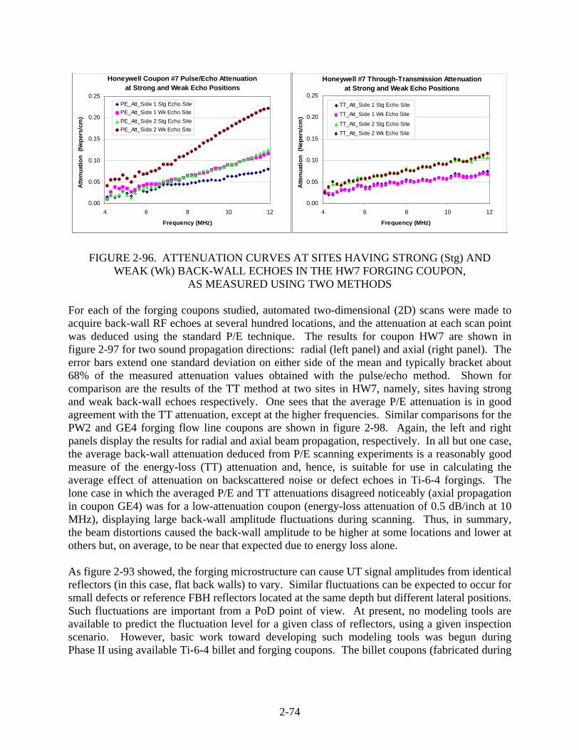
2-74

FIGURE 2-96. ATTENUATION CURVES AT SITES HAVING STRONG (Stg) AND WEAK (Wk) BACK-WALL ECHOES IN THE HW7 FORGING COUPON,

AS MEASURED USING TWO METHODS

For each of the forging coupons studied, automated two-dimensional (2D) scans were made to acquire back-wall RF echoes at several hundred locations, and the attenuation at each scan point was deduced using the standard P/E technique. The results for coupon HW7 are shown in figure 2-97 for two sound propagation directions: radial (left panel) and axial (right panel). The error bars extend one standard deviation on either side of the mean and typically bracket about 68% of the measured attenuation values obtained with the pulse/echo method. Shown for comparison are the results of the TT method at two sites in HW7, namely, sites having strong and weak back-wall echoes respectively. One sees that the average P/E attenuation is in good agreement with the TT attenuation, except at the higher frequencies. Similar comparisons for the PW2 and GE4 forging flow line coupons are shown in figure 2-98. Again, the left and right panels display the results for radial and axial beam propagation, respectively. In all but one case, the average back-wall attenuation deduced from P/E scanning experiments is a reasonably good measure of the energy-loss (TT) attenuation and, hence, is suitable for use in calculating the average effect of attenuation on backscattered noise or defect echoes in Ti-6-4 forgings. The lone case in which the averaged P/E and TT attenuations disagreed noticeably (axial propagation in coupon GE4) was for a low-attenuation coupon (energy-loss attenuation of 0.5 dB/inch at 10 MHz), displaying large back-wall amplitude fluctuations during scanning. Thus, in summary, the beam distortions caused the back-wall amplitude to be higher at some locations and lower at others but, on average, to be near that expected due to energy loss alone. As figure 2-93 showed, the forging microstructure can cause UT signal amplitudes from identical reflectors (in this case, flat back walls) to vary. Similar fluctuations can be expected to occur for small defects or reference FBH reflectors located at the same depth but different lateral positions. Such fluctuations are important from a PoD point of view. At present, no modeling tools are available to predict the fluctuation level for a given class of reflectors, using a given inspection scenario. However, basic work toward developing such modeling tools was begun during Phase II using available Ti-6-4 billet and forging coupons. The billet coupons (fabricated during

Honeywell Coupon #7 Pulse/Echo Attenuationat Strong and Weak Echo Positions

0.00

0.05

0.10

0.15

0.20

0.25

4 6 8 10 12

Frequency (MHz)

Atte

nuat

ion

(Nep

ers/

cm)

PE_Att_Side 1 Stg Echo SitePE_Att_Side 1 Wk Echo SitePE_Att_Side 2 Stg Echo SitePE_Att_Side 2 Wk Echo Site

Honeywell #7 Through-Transmission Attenuationat Strong and Weak Echo Positions

0.00

0.05

0.10

0.15

0.20

0.25

4 6 8 10 12

Frequency (MHz)

Atte

nuat

ion

(Nep

ers/

cm)

TT_Att_Side 1 Stg Echo Site

TT_Att_Side 1 Wk Echo Site

TT_Att_Side 2 Stg Echo SiteTT_Att_Side 2 Wk Echo Site

Honeywell Coupon #7 Pulse/Echo Attenuationat Strong and Weak Echo Positions

0.00

0.05

0.10

0.15

0.20

0.25

4 6 8 10 12

Frequency (MHz)

Atte

nuat

ion

(Nep

ers/

cm)

PE_Att_Side 1 Stg Echo SitePE_Att_Side 1 Wk Echo SitePE_Att_Side 2 Stg Echo SitePE_Att_Side 2 Wk Echo Site

Honeywell #7 Through-Transmission Attenuationat Strong and Weak Echo Positions

0.00

0.05

0.10

0.15

0.20

0.25

4 6 8 10 12

Frequency (MHz)

Atte

nuat

ion

(Nep

ers/

cm)

TT_Att_Side 1 Stg Echo Site

TT_Att_Side 1 Wk Echo Site

TT_Att_Side 2 Stg Echo SiteTT_Att_Side 2 Wk Echo Site

2-75

FIGURE 2-97. MEASURED ATTENUATION OF Ti-6-4 FORGING COUPON HW7 AS DEDUCED FROM P/E BACK-WALL SCANS (PLOTTED POINTS

WITH ERROR BARS) AND FROM THE TT METHOD (AT STRONG AND WEAK ECHO SITES)

FIGURE 2-98. MEASURED ATTENUATION OF Ti-6-4 FORGING COUPONS PW2 AND GE4 AS DEDUCED FROM P/E BACK-WALL SCANS (PLOTTED

POINTS WITH ERROR BARS) AND FROM THE TT METHOD (AT STRONG AND WEAK ECHO SITES)

Attenuation of Coupon HW7 (Radial Propagation)

0.00

0.01

0.02

0.03

0.04

0.05

0.06

0.07

0.08

0.09

2 4 6 8 10 12

Frequency (MHz)

Atte

nuat

ion

(Nep

ers/

cm) P/E C-scan_Side 1

TT_Att_Stg_SiteTT_Att_Wk_Site

Attenuation of Coupon HW7 (Axial Propagation)

0.00

0.02

0.04

0.06

0.08

0.10

0.12

0.14

0.16

0.18

2 4 6 8 10 12

Frequency (MHz)

Atte

nuat

ion

(Nep

ers/

cm)

P/E C-scan_Side 2TT_Att_Stg_SiteTT_Att_Wk_Site

Attenuation of Coupon HW7 (Radial Propagation)

0.00

0.01

0.02

0.03

0.04

0.05

0.06

0.07

0.08

0.09

2 4 6 8 10 12

Frequency (MHz)

Atte

nuat

ion

(Nep

ers/

cm) P/E C-scan_Side 1

TT_Att_Stg_SiteTT_Att_Wk_Site

Attenuation of Coupon HW7 (Axial Propagation)

0.00

0.02

0.04

0.06

0.08

0.10

0.12

0.14

0.16

0.18

2 4 6 8 10 12

Frequency (MHz)

Atte

nuat

ion

(Nep

ers/

cm)

P/E C-scan_Side 2TT_Att_Stg_SiteTT_Att_Wk_Site

Attenuation of Coupon PW2 (Radial Propagation)

0.00

0.02

0.04

0.06

0.08

2 4 6 8 10 12

Frequency (MHz)

Atte

nuat

ion

(Nep

ers/

cm)

P/E C-scan_Side 1TT_Att_Stg_SiteTT_Att_Wk_Site

Attenuation of Coupon PW2 (Axial Propagation)

0.00

0.02

0.04

0.06

0.08

2 4 6 8 10 12

Frequency (MHz)

Atte

nuat

ion

(Nep

ers/

cm)

P/E C-scan_Side 2TT_Att_Stg_SiteTT_Att_Wk_Site

Attenuation of Coupon GE4 (Radial Propagation)

0.00

0.02

0.03

0.05

0.06

2 4 6 8 10 12

Frequency (MHz)

Atte

nuat

ion

(Nep

ers/

cm)

P/E C-scan_Side 1TT_Att_Stg_SiteTT_Att_Wk_Site

Attenuation of Coupon GE4 (Axial Propagation)

0.00

0.02

0.03

0.05

0.06

2 4 6 8 10 12

Frequency (MHz)

Atte

nuat

ion

(Nep

ers/

cm)

P/E C-scan_Side 2TT_Att_Stg_SiteTT_Att_Wk_Site

Attenuation of Coupon PW2 (Radial Propagation)

0.00

0.02

0.04

0.06

0.08

2 4 6 8 10 12

Frequency (MHz)

Atte

nuat

ion

(Nep

ers/

cm)

P/E C-scan_Side 1TT_Att_Stg_SiteTT_Att_Wk_Site

Attenuation of Coupon PW2 (Axial Propagation)

0.00

0.02

0.04

0.06

0.08

2 4 6 8 10 12

Frequency (MHz)

Atte

nuat

ion

(Nep

ers/

cm)

P/E C-scan_Side 2TT_Att_Stg_SiteTT_Att_Wk_Site

Attenuation of Coupon GE4 (Radial Propagation)

0.00

0.02

0.03

0.05

0.06

2 4 6 8 10 12

Frequency (MHz)

Atte

nuat

ion

(Nep

ers/

cm)

P/E C-scan_Side 1TT_Att_Stg_SiteTT_Att_Wk_Site

Attenuation of Coupon GE4 (Axial Propagation)

0.00

0.02

0.03

0.05

0.06

2 4 6 8 10 12

Frequency (MHz)

Atte

nuat

ion

(Nep

ers/

cm)

P/E C-scan_Side 2TT_Att_Stg_SiteTT_Att_Wk_Site

2-76

ETC Phase I) were preferred for some of the initial experiments because signal fluctuation levels tended to be larger and, thus, more easily measured. The underlying central concept for model development is that the fluctuations for different types of reflectors (e.g., back walls or FBHs) all stem from distortions of the propagating sound beam by the microstructure. Thus, if a few key statistical parameters that describe the nature and severity of the beam distortions can be defined and measured, then these can be used as inputs to models that predict the signal fluctuations. The distortion parameters currently being considered provide statistical descriptions of (1) the lateral drift of the center of energy about its expected position (beam skewing), (2) the distortion of pressure amplitude about its expected pattern, and (3) two types of wavefront distortion (wrinkling and tilting). The meanings of these beam distortion categories are illustrated in figure 2-99.

FIGURE 2-99. CATEGORIES OF UT PRESSURE-FIELD DISTORTIONS TREATED IN SIGNAL FLUCTUATION MODELS

An effort was initiated [33 and 34] to develop models that relate the fluctuations in back-wall amplitude C-scans (like those of figure 2-93) to sonic beam distortions as measured via TT beam mapping (like those of figure 2-95). First it was shown that the back-wall echo at a particular location in a Ti alloy specimen could be accurately predicted from TT beam-mapping data at that same location. This is illustrated in figure 2-100 for measurements made on a 2″ thick block cut from a Ti-17 billet. The billet specimen was inspected in the axial direction using a 5-MHz,

Distortions of sonic wavefronts

• Systematic tilting: ? .

• Phase “wrinkling”: ΔΦ .

Distortions of the lateral amplitude profile

• Drift of center of energy: ΔD.

• Amplitude “wrinkling”: ΔA/A0.

ΔA A0

?

ΔΦ

ΔD

Sonic field for a Homogeneous Microstructure

Distorted field for an inhomogeneousMicrostructure

Distortions of sonic wavefronts

• Systematic tilting: ? .

• Phase “wrinkling”: ΔΦ .

Distortions of the lateral amplitude profile

• Drift of center of energy: ΔD.

• Amplitude “wrinkling”: ΔA/A0.

ΔA A0ΔA A0ΔA A0

???

ΔΦΔΦΔΦ

ΔDΔD

Sonic field for a Homogeneous Microstructure

Distorted field for an inhomogeneousMicrostructure

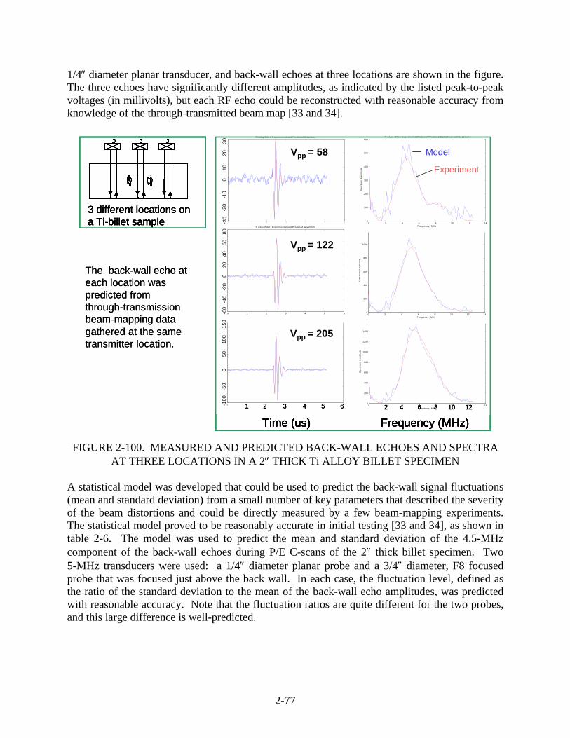
2-77

1/4″ diameter planar transducer, and back-wall echoes at three locations are shown in the figure. The three echoes have significantly different amplitudes, as indicated by the listed peak-to-peak voltages (in millivolts), but each RF echo could be reconstructed with reasonable accuracy from knowledge of the through-transmitted beam map [33 and 34]. FIGURE 2-100. MEASURED AND PREDICTED BACK-WALL ECHOES AND SPECTRA

AT THREE LOCATIONS IN A 2″ THICK Ti ALLOY BILLET SPECIMEN A statistical model was developed that could be used to predict the back-wall signal fluctuations (mean and standard deviation) from a small number of key parameters that described the severity of the beam distortions and could be directly measured by a few beam-mapping experiments. The statistical model proved to be reasonably accurate in initial testing [33 and 34], as shown in table 2-6. The model was used to predict the mean and standard deviation of the 4.5-MHz component of the back-wall echoes during P/E C-scans of the 2″ thick billet specimen. Two 5-MHz transducers were used: a 1/4″ diameter planar probe and a 3/4″ diameter, F8 focused probe that was focused just above the back wall. In each case, the fluctuation level, defined as the ratio of the standard deviation to the mean of the back-wall echo amplitudes, was predicted with reasonable accuracy. Note that the fluctuation ratios are quite different for the two probes, and this large difference is well-predicted.

3 different locations ona Ti-billet sample

0 1 2 3 4 5 6-100

-50

0

50

100

150Ti A lloy B illet : Experimental and P redicted W aveform

0 2 4 6 8 10 12 140

200

400

600

800

1000

1200

1400

1600

Frequency, M Hz

Spe

ctru

m A

mpl

itude

Ti ALloy Billet: Experim ental(Red) and Predic ted Back(Blue) wall Spectrum

0 2 4 6 8 10 12 140

200

400

600

800

1000

1200

Frequency, MHz

Spe

ctru

m A

mpl

itude

Ti ALloy Billet: Experimental(Red) and Predicted Back(Blue) wall Spectrum

0 1 2 3 4 5 6-30

-20

-10

0

10

20

30Ti A lloy B illet : Experim ental and P redicted W aveform

0 1 2 3 4 5 6-60

-40

-20

0

20

40

60

80Ti Alloy Billet: Experimental and P redicted W aveform

0 2 4 6 8 10 12 140

100

200

300

400

500

600

Frequency, MHz

Spe

ctru

m A

mpl

itude

Ti ALloy B illet: Experimental(Red) and P redic ted Back(B lue) wall Spectrum

Time (us) Frequency (MHz)2 4 6 8 10 121 2 3 4 5 6

-10

-30

-20

010

2030

-20

-60

-40

020

4060

80-1

00-5

00

5010

015

0

Vpp = 58

Vpp = 122

Vpp = 205

The back-wall echo at each location was predicted from through-transmission beam-mapping data gathered at the same transmitter location.

Experiment

Model

3 different locations ona Ti-billet sample3 different locations ona Ti-billet sample3 different locations ona Ti-billet sample

0 1 2 3 4 5 6-100

-50

0

50

100

150Ti A lloy B illet : Experimental and P redicted W aveform

0 2 4 6 8 10 12 140

200

400

600

800

1000

1200

1400

1600

Frequency, M Hz

Spe

ctru

m A

mpl

itude

Ti ALloy Billet: Experim ental(Red) and Predic ted Back(Blue) wall Spectrum

0 2 4 6 8 10 12 140

200

400

600

800

1000

1200

Frequency, MHz

Spe

ctru

m A

mpl

itude

Ti ALloy Billet: Experimental(Red) and Predicted Back(Blue) wall Spectrum

0 1 2 3 4 5 6-30

-20

-10

0

10

20

30Ti A lloy B illet : Experim ental and P redicted W aveform

0 1 2 3 4 5 6-60

-40

-20

0

20

40

60

80Ti Alloy Billet: Experimental and P redicted W aveform

0 2 4 6 8 10 12 140

100

200

300

400

500

600

Frequency, MHz

Spe

ctru

m A

mpl

itude

Ti ALloy B illet: Experimental(Red) and P redic ted Back(B lue) wall Spectrum

Time (us) Frequency (MHz)2 4 6 8 10 121 2 3 4 5 6

-10

-30

-20

010

2030

-20

-60

-40

020

4060

80-1

00-5

00

5010

015

0

Vpp = 58

Vpp = 122

Vpp = 205

0 1 2 3 4 5 6-100

-50

0

50

100

150Ti A lloy B illet : Experimental and P redicted W aveform

0 2 4 6 8 10 12 140

200

400

600

800

1000

1200

1400

1600

Frequency, M Hz

Spe

ctru

m A

mpl

itude

Ti ALloy Billet: Experim ental(Red) and Predic ted Back(Blue) wall Spectrum

0 2 4 6 8 10 12 140

200

400

600

800

1000

1200

Frequency, MHz

Spe

ctru

m A

mpl

itude

Ti ALloy Billet: Experimental(Red) and Predicted Back(Blue) wall Spectrum

0 1 2 3 4 5 6-30

-20

-10

0

10

20

30Ti A lloy B illet : Experim ental and P redicted W aveform

0 1 2 3 4 5 6-60

-40

-20

0

20

40

60

80Ti Alloy Billet: Experimental and P redicted W aveform

0 2 4 6 8 10 12 140

100

200

300

400

500

600

Frequency, MHz

Spe

ctru

m A

mpl

itude

Ti ALloy B illet: Experimental(Red) and P redic ted Back(B lue) wall Spectrum

Time (us) Frequency (MHz)2 4 6 8 10 121 2 3 4 5 6

-10

-30

-20

010

2030

-20

-60

-40

020

4060

80-1

00-5

00

5010

015

0

0 1 2 3 4 5 6-100

-50

0

50

100

150Ti A lloy B illet : Experimental and P redicted W aveform

0 2 4 6 8 10 12 140

200

400

600

800

1000

1200

1400

1600

Frequency, M Hz

Spe

ctru

m A

mpl

itude

Ti ALloy Billet: Experim ental(Red) and Predic ted Back(Blue) wall Spectrum

0 2 4 6 8 10 12 140

200

400

600

800

1000

1200

Frequency, MHz

Spe

ctru

m A

mpl

itude

Ti ALloy Billet: Experimental(Red) and Predicted Back(Blue) wall Spectrum

0 1 2 3 4 5 6-30

-20

-10

0

10

20

30Ti A lloy B illet : Experim ental and P redicted W aveform

0 1 2 3 4 5 6-60

-40

-20

0

20

40

60

80Ti Alloy Billet: Experimental and P redicted W aveform

0 2 4 6 8 10 12 140

100

200

300

400

500

600

Frequency, MHz

Spe

ctru

m A

mpl

itude

Ti ALloy B illet: Experimental(Red) and P redic ted Back(B lue) wall Spectrum

Time (us) Frequency (MHz)2 4 6 8 10 121 2 3 4 5 6

Time (us) Frequency (MHz)2 4 6 8 10 122 4 6 8 10 121 2 3 4 5 61 2 3 4 5 6

-10

-30

-20

010

2030

-10

-30

-20

010

2030

-20

-60

-40

020

4060

80-2

0-6

0-4

00

2040

6080

-100

-50

050

100

150

-100

-50

050

100

150

Vpp = 58

Vpp = 122

Vpp = 205

The back-wall echo at each location was predicted from through-transmission beam-mapping data gathered at the same transmitter location.

Experiment

Model

2-78

TABLE 2-6. MEASURED AND PREDICTED SPECTRAL AMPLITUDE CHARACTERISTICS

Probe Type Measured Predicted Mean (μ) 613.32 664.53 STD (σ) 158.92 201.20

Planar probe

σ/μ 25.92% 30.28% Mean (μ) 1249.42 1056.65 STD (σ) 73.25 53.75

Focused probe

σ/μ 5.87% 5.09%

STD = Standard deviation In addition, a parallel effort was begun to make use of a 2D computational model [35] that predicts sonic beam patterns in the presence of microstructures. For several types of model microstructures containing elongated grains, the 2D model was used to predict distorted beams for many ensembles of grains and to predict the back-wall amplitude for each grain ensemble. In experimental terms, this calculation would be equivalent to measuring the back-wall response for a P/E inspection at several hundred locations above a specimen, and then mapping the through-transmitted beam (using a small-diameter receiver) at each location. The computed distorted beams were then analyzed to obtain the beam distortion severity parameters, which were input into the statistical model to predict the back-wall echo fluctuations. The predictions were found to be in generally good agreement with the characteristics of back-wall echoes, as calculated directly for each model microstructure [35]. Although all work to date for the statistical model has been for single-frequency components of the UT data, the extension to full RF signals should be possible. The details of the signal fluctuation model development were presented at the July 2003 QNDE Conference in Green Bay, WI, see references 33 and 35. 2.2.7 Summary.

Each of the three OEMs selected a representative Ti-6-4 engine forging and performed focused-probe, normal incident, P/E C-scans to map out backscattered grain noise patterns in the forging interior. Each OEM also provided a cross-sectional macroetch of the forging, revealing flow line patterns, and DEFORM calculations of metal strain, which developed during the forging process. From the noise maps, macroetches, and DEFORM calculations, coupon sites were selected within each forging. In the circumferential direction of each forging, coupons were cut from high-noise sectors since high-noise regions are generally the most difficult to inspect. Within the high-noise sector, coupon locations in the axial and radial directions were generally chosen to span the widest possible range of microstructures. A total of 26 such coupons were cut. The majority (20) being rectangular blocks of standard size with nominal dimensions of 1.25″ by 1.25″ by 2.0″ (radial by axial by hoop). Three of the coupons were cylinders used to study the dependence of grain noise on inspection direction. Systematic P/E, longitudinal-wave UT property measurements of the standard blocks were performed at two facilities. Velocity, attenuation, and backscattered noise measurements were

2-79

performed at ISU for all 20 standard-sized coupons for beam propagation in the radial and axial directions (the usual propagation directions for longitudinal-wave forging inspections). Similar (but not always identical) measurements were performed for radial, axial, and hoop propagation on eight standard-sized coupons from the P&W forging by P&W personnel. The measurements at the two facilities were in good general agreement. For all three OEM forgings, sonic velocity variations were quite small, usually varying by less that 1 percent with position and inspection direction. Although the variations were small, systematic changes in velocity and velocity anisotropy was observed as one moved from the ID to the OD of a given forging. By themselves, these small variations in average sound speed are believed to pose no particular inspection difficulties. By contrast, variations of the UT attenuation and the average backscattered grain noise with position and inspection direction in the radial-axial plane were quite large, with either quantity varying significantly within a given forging by about an order of magnitude within the suite of forging flow line coupons. Measured attenuation values at 10 MHz ranged from 0.2 to 2.7 dB/inch, and maximal GPN levels ranged from 0.5% to 6.9% of the amplitude of a #1 FBH reference reflector. The N/S values quoted above are specifically for an inspection using a focused transducer having a sonic PV of 2.2E-5 cubic inches; N/S ratios for other inspections can be estimated by using a rule of thumb that relates N/S to the square root of the PV. Variations of noise and attenuation with position and inspection direction were found to be related to one another and to the details of the local forging strain. At a given location in a forging, the direction in which the measured noise was greatest was generally the direction in which the measured attenuation was smallest. The maximal noise, minimal attenuation direction generally occurred for beam propagation perpendicular to the macrostructure elongation direction (i.e., the flow lines). The noise (or attenuation) anisotropy, defined as the noise (or attenuation) measured for axial propagation divided by that measured for radial propagation, was well correlated with the local forging strain, as calculated by the DEFORM software. More specifically, DEFORM calculations were performed in which circular or ellipsoidal volume elements in the billet (model macrograins) were tracked to determine their final shapes at the conclusion of the forging process. The noise or attenuation anisotropy was found to be well correlated with the ratio of the projections of the forging macrograins onto the two inspection directions. The clear relationship between noise anisotropy and forging macrograin geometry (as calculated using DEFORM) led to an effort at ISU to develop two models to predict the variation of absolute grain noise levels within a forging. The simpler model version treats the forging as an effective scattering medium described by two global parameters, which are the same at all points in the forging. One parameter describes the average size of the forging macrograins, and the other describes the average difference in elastic stiffness constants from one macrograin to the next. The model relies on DEFORM to calculate the shapes and orientations of the macrograins at various locations in the forging, assuming the initial macrograins in the billet are elongated in the axial direction. The simpler version of the model assumes the crystalline axes within the macrograins are randomly oriented. The more complex version of the model takes into account the preferred orientations (texture) that develop in high-strain regions. Both models were applied

2-80

to predict noise variations throughout the P&W forging, showing reasonable agreement with experiment. This suggests that noise variations within forgings can be largely understood by following the shapes and orientations of the metal macrograins during the forging process. Backscattered grain noise can mask the echo from a small or subtle defect in a forging, thus playing a key role in determining the defect detection limits. Although all the forging flow line coupons were cut from high-noise sections of the OEM-supplied forgings, some coupons had higher grain noise levels than others. Additional measurements were performed on three coupons (one from each forging) having the largest absolute noise levels. In particular, the backscattered grain noise capacity (or FOM) was measured as a function of frequency for various depth zones and tabulated for the zone having the maximum FOM value. The values of velocity, attenuation, and noise FOM for these three worst-case microstructures can be used as inputs to inspection simulation models, which estimate the PoD for various forging inspection schemes. Current forging inspections are generally designed to #1 FBH sensitivity, i.e., to reliably detect any defect whose reflectivity exceeds that of a #1 FBH. A four-fold improvement in detection amplitude to a #1/2 FBH standard is desired for future forging inspections. The three high-noise coupons were used to determine beam focal requirements for achieving the #1/2 FBH detection sensitivity. As the sonic beam becomes better focused, the peak S/N ratio for a given defect tends to rise, being approximately proportional the reciprocal of the square-root of the sonic PV at the defect’s location. At the GE facility in Cincinnati, OH, S/N ratios for the three high-noise coupons were repeatedly measured using different 10-MHz transducers and various water path choices to span a wide range of PVs. #1 FBH reflectors were drilled into the high-noise coupons to facilitate these measurements. These results indicated that a typical 10-MHz forging inspection, which meets the #1/2 FBH sensitivity target, requires a beam diameter that does not exceed about 45 mils at any depth within a given inspection zone. This information was used in the Inspection Development for Titanium Forging Study to design improved forging inspection schemes. Selected forging flow line coupons were used to study UT signal fluctuations caused by the metal microstructure. For example, the amplitude of a back-wall echo can fluctuate noticeably over relatively short distances, giving back-wall amplitude C-scan images a speckled appearance. These fluctuations have important implications for PoD. To study the fluctuations, a small receiving transducer (pinducer) was used to map the amplitude and phase profiles of sonic beams that emerged after passing through Ti alloy and FQ blocks. It was shown that distortions of the profiles by the Ti microstructure were responsible for the variation in the back-wall amplitude when the transmitting probe was scanned in P/E mode. The beam profile maps were also used to measure the energy-loss attenuation in selected forging flow line coupons. For these coupons, the average attenuation value deduced from planar probe P/E measurements of back-wall amplitude was generally close to the energy-loss value. Thus, the beam distortions caused the back-wall amplitude to be higher at some locations and lower at others, but on average, near that expected due to energy loss alone. Work was also begun on the development of a model that could predict the back-wall signal fluctuation level from several model parameters that described the nature and severity of the

2-81

beam distortions, with those model parameters themselves measured via TT beam-mapping experiments. Initial tests of the model formalism, both experimentally and through computer simulations, appeared promising. 2.3 EFFECT OF SURFACE CURVATURE ON INSPECTABILITY.

Real-world forgings have complex geometries that can impact inspection sensitivity. If a component being inspected has a curved sound-entry surface, the shape of the sonic beam injected into the interior is altered compared to a flat-entry surface. For example, a focused sound beam may focus deeper or shallower under a curved surface, and the focal spot may have an elliptical rather than a circular cross section. Such modifications in the shape of the incident UT field affect inspections in two basic ways: (1) the sonic pressure field incident upon a flaw is altered, changing both the peak flaw amplitude and the shape and size of the defect image within a C-scan and (2) since the cross section of the sonic beam is changed, a different collection of metal grains will be insonified, thus altering the backscattered grain noise level. These two phenomena together determine S/N ratios and, hence, defect detection probabilities. Models have been developed at ISU to treat the effects of surface curvature on both defect signal amplitude [7] and backscattered grain noise characteristics. (See Appendix B of reference 16.) Two classes of specimens containing both convex and concave upper surfaces were fabricated to study the effect of surface curvature on disk inspections and to test model predictions. A set of six specimens known as curvature correction blocks were made from an ultrasonically neutral material, i.e., fine-grained Ni alloy R88DT. These were used to measure the effect of surface curvature on FBH signal amplitudes at various depths. The R88DT material was chosen so that the effect of surface curvature on FBH amplitudes could be studied in the absence of backscattered grain noise. A second set of six blocks with curved upper surfaces was machined from a representative Ti-6-4 forged disk. These blocks are referred to as noise curvature blocks, and were primarily used to measure the effect of surface curvature on backscattered grain noise levels. The measurements performed on both sets of blocks are discussed below along with comparisons to model predictions. 2.3.1 Effect of Surface Curvature on FBH Amplitudes.

Before curvature correction blocks were fabricated, the Consortium OEMs were surveyed to determine the range of surface curvatures likely to be encountered during inspections of the sonic shapes of current and future forgings. It was determined that convex radii with a curvature of 4″ and larger and a concave radii of 0.75″ and larger were of chief interest. The research team then decided that convex radii of 4.0″ and 8.0″ and concave radii of 0.75″, 2.0″, and 8.0 would be reasonable choices for the test block curvatures. Prior to fabricating the blocks, model calculations were performed to assess the likely effect of each curvature choice on inspectability. This was done to check that each selected curvature would lead to an easily measurable, but not overly extreme, change in defect amplitudes compared to a flat-entry surface. The inspection parameters assumed in the model simulations are listed below. Two commonly used inspection scenarios were examined, each of which used spherically focused, 10-MHz transducers. In the first case a 3/8″ diameter transducer was focused near the entry surface; in the second case, a 3/4″ diameter transducer was focused well into the interior. Model defects were FBHs with

2-82

20-mil diameters located at a sequence of depths down to 2″. The specimens were assumed to be made from generic Ti-6-4 forging material, having velocity and attenuation values typical of those measured earlier in the forging flow line coupons. The responses from the FBHs were calculated using the Thompson-Gray measurement model with a Gauss-Hermite expansion for the incident sonic beam [7, 20, and 36]. • Transducers

− 10 MHz, 3/8″ diameter, 3″ focal length. Focused near the entry surface. − 10 MHz, 3/4″ diameter, 8″ focal length. Focused 1″ below the entry surface.

• Surface Radii of Curvature

− Flat − Concave: 0.75″, 2.0″, and 8.0″ − Convex: 4.0″ and 10.0″

• Size of FBH: 0.020″ diameter • Depth of holes was varied from 0.050″ to 2.0″ with 0.005″ steps • ISU model applied (Thompson/Gray) • Ti-6-4 generic velocity and attenuation assumed

Figure 2-101 displays the results of model calculations for the case where the sonic beam is focused near the entry surface. The upper panels in the figure show the predicted absolute FBH amplitudes (in arbitrary units) as a function of depth for a flat-entry surface and for each of the five assumed surface curvatures. The predicted amplitude for a (smaller) #1 FBH below a flat surface is also shown for comparison. The lower panels in figure 2-101 show the differences (in dB units) between the predicted FBH amplitudes beneath each curved surface and the FBH amplitude beneath a flat surface. As expected, the difference grows as the surface curvature becomes more severe, i.e., as the magnitude of the radius of curvature decreases. For the near-surface focus case, the predicted amplitude differences, relative to the flat surface, range from about -10 dB to +10 dB. Figure 2-102 displays similar results for the other case considered, where the water path was fixed such that the nominal focus would occur about 1″ deep for a flat-surface inspection. For the simulated inspection through the flat surface, the focal maximum is found to be somewhat inside the 1″, due to both the effect of metal attenuation and the fact that the actual focal point of a transducer is always inside the geometric focal point (where the beam would focus in the absence of sound diffraction). For concave curvatures, the beam focuses at shallower depths, and for convex curvatures, it focuses at deeper depths. The departures of the predicted FBH amplitudes from the flat-surface case range from about -28 dB to +28 dB over the 2″ depth range. Again, the departures are larger when the surface curvature is more severe. It was noted that the predicted dB difference curves shown in figures 2-101 and 2-102 are relatively insensitive to the diameter of the FBH, so long as the hole is small compared to the lateral width of the beam.

2-83

FIGURE 2-101. CALCULATED RESPONSES FROM 20-mil-DIAMETER FBHs LOCATED

BELOW FLAT AND CURVED SURFACES IN Ti-6-4 FORGING MATERIAL (BEAM FOCUSED NEAR SURFACE)

FIGURE 2-102. CALCULATED RESPONSES FROM 20-mil-DIAMETER FBHs LOCATED BELOW FLAT AND CURVED SURFACES IN Ti-6-4 FORGING MATERIAL (BEAM

FOCUSED BELOW SURFACE)

E ffect of c oncave su rface 10 MHz , 3" focus p robe, focused near surface

0.0

10 .0

20 .0

30 .0

40 .0

50 .0

60 .0

0.0 0.5 1 .0 1.5 2.0

Hole Depth, in

Am

plitu

de

#1F BH, flat

20 mils, flat

20 mils, 0.75" concave

20 mi ls, 2" c oncave

20 mi ls, 8" c oncave

E ffec t o f concave surface 10 MH z , 3" focus p robe, focuse d near surface

Amp litude change comp ared to fla t

-15

-10

-5

0

5

10

15

0.00 0.50 1.00 1.50 2.00

Hole Depth, in

Am

plit

ude

ch

ang

e, d

B

0.75" concave

2" c oncave

8" c oncave

E ffect of co nvex surface 10 MHz, 3" focus p robe, focused near surface

0

5

10

15

20

25

30

0.00 0.50 1.00 1.50 2.00Hole Depth, in

Am

plitu

de

#1FBH, flat

20 mils , f lat

20 mils , 4" convex

20 mils , 10" c onvex

Effect o f con vex surface 10 MHz , 3" focu s probe , focus ed near surfac e

Am plitude cha nge compared to flat

-2 .00

-1.50

-1.00

-0.50

0.00

0.50

1.00

1.50

2.00

0 .00 0 .50 1 .00 1 .50 2.00

Hole Depth , inA

mpl

itud

e ch

ang

e, d

B 4" convex

10" convex

Effect of concave surface 10 M Hz , 8" focu s probe, focuse d @ 1"

0.000

0 .002

0 .004

0 .006

0 .008

0.0 0.5 1.0 1.5 2.0

Depth , in

FB

H r

esp

onc

e

flat s urfac e

0.7 5" co nca ve

2" concave

8" concave

Effect o f concave s urface 10 MH z, 8" focus pro be, focused @ 1"

Am p litude change comp ared to flat

-30

-20

-10

0

10

20

30

0.0 0.5 1.0 1.5 2.0

De pth , in

Diff

eren

ce (c

onve

x-fla

t),

dB

0 .75" concave

2" co nca ve

8" co nca ve

E ffect of con vex surfac e 10 MH z, 8" fo cus probe, focus ed @ 1"

0.00 0

0.00 1

0.00 2

0.00 3

0.00 4

0.00 5

0.00 6

0.00 7

0. 0 0. 5 1.0 1. 5 2. 0

D epth , in

FB

H r

esp

once

f lat surfac e

4" c onvex

10" conve x

E ffect of con vex s urface 1 0 M Hz , 8" focus probe, focused @ 1"

Amplitude cha ng e c om pared to flat

-10

-8

-6

-4

-2

0

2

0.0 0.5 1.0 1.5 2.0

Depth, in

Diff

eren

ce (c

onve

x-fl

at),

dB

4" c onve x

10" c onve x

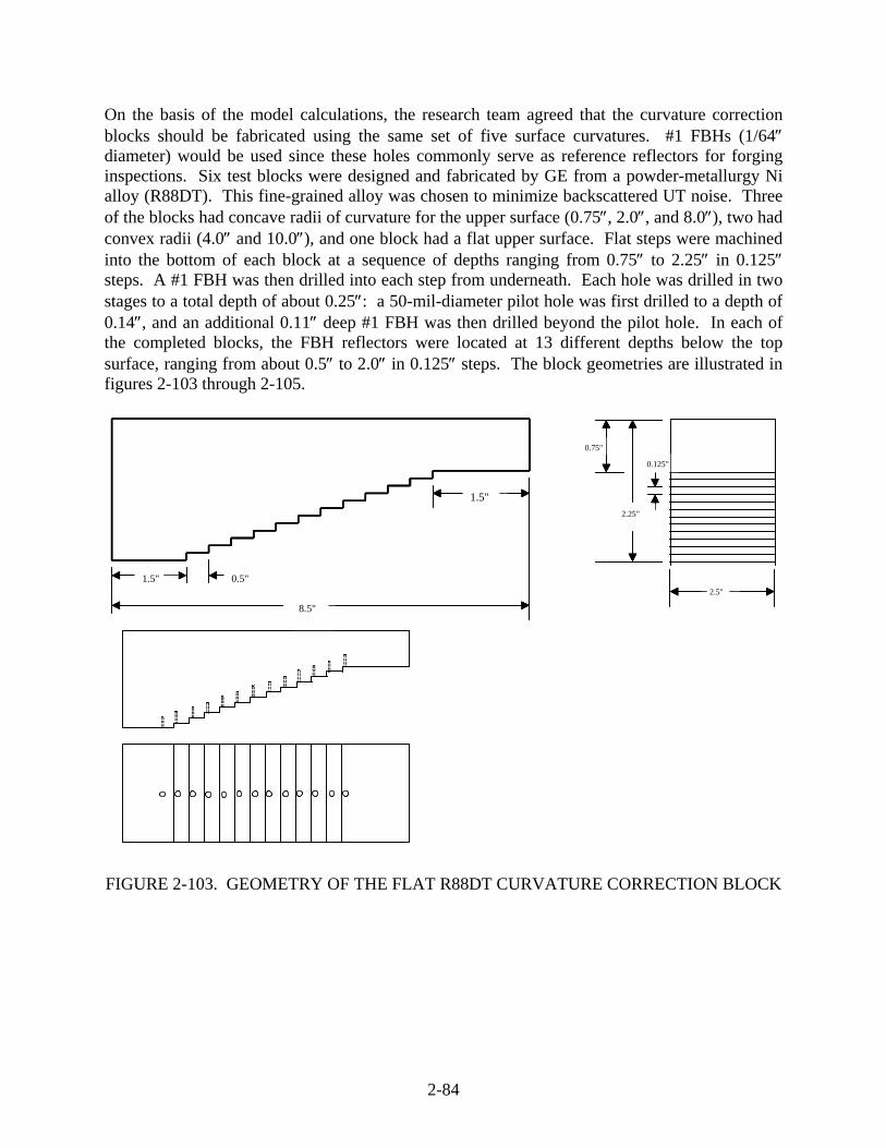
2-84

On the basis of the model calculations, the research team agreed that the curvature correction blocks should be fabricated using the same set of five surface curvatures. #1 FBHs (1/64″ diameter) would be used since these holes commonly serve as reference reflectors for forging inspections. Six test blocks were designed and fabricated by GE from a powder-metallurgy Ni alloy (R88DT). This fine-grained alloy was chosen to minimize backscattered UT noise. Three of the blocks had concave radii of curvature for the upper surface (0.75″, 2.0″, and 8.0″), two had convex radii (4.0″ and 10.0″), and one block had a flat upper surface. Flat steps were machined into the bottom of each block at a sequence of depths ranging from 0.75″ to 2.25″ in 0.125″ steps. A #1 FBH was then drilled into each step from underneath. Each hole was drilled in two stages to a total depth of about 0.25″: a 50-mil-diameter pilot hole was first drilled to a depth of 0.14″, and an additional 0.11″ deep #1 FBH was then drilled beyond the pilot hole. In each of the completed blocks, the FBH reflectors were located at 13 different depths below the top surface, ranging from about 0.5″ to 2.0″ in 0.125″ steps. The block geometries are illustrated in figures 2-103 through 2-105. FIGURE 2-103. GEOMETRY OF THE FLAT R88DT CURVATURE CORRECTION BLOCK

0.125"

1.5"

1.5"

8.5"

0.5"

0.75"

2.25"

2.5"

0.125"

1.5"

1.5"

8.5"

0.5"

0.75"

2.25"

2.5"

0.125"

1.5"

1.5"

8.5"

0.5"

0.75"

2.25"

2.5"

2-85

FIGURE 2-104. GEOMETRY OF THE R88DT CURVATURE CORRECTION BLOCK WITH A 10″ CONVEX CURVATURE

(See figure 2-103 for drilled holes.)

FIGURE 2-105. GEOMETRY OF THE R88DT CURVATURE CORRECTION BLOCK WITH AN 8″ CONCAVE CURVATURE AND PERTINENT DIMENSIONS FOR

THE OTHER CONCAVE BLOCKS (See figure 2-103 for drilled holes.)

1.5"

1.5"

8.5"

0.5"

0.75"

C = 0.098”

H = 2.348”

R = 8”

W

0.125"

2.50”

2.503.251.50W

0.1250.1250.125S

2.3483.0853.00H

0.0980.8340.75C

8.02.00.75R

2.503.251.50W

0.1250.1250.125S

2.3483.0853.00H

0.0980.8340.75C

8.02.00.75R

1.5"

1.5"

8.5"

0.5"

0.75"

C = 0.098”

H = 2.348”

R = 8”

W

0.125"

2.50”

1.5"

1.5"

8.5"

0.5"

0.75"

C = 0.098”

H = 2.348”

R = 8”

W

0.125"

2.50”

2.503.251.50W

0.1250.1250.125S

2.3483.0853.00H

0.0980.8340.75C

8.02.00.75R

2.503.251.50W

0.1250.1250.125S

2.3483.0853.00H

0.0980.8340.75C

8.02.00.75R

1.5"

1.5"

8.5"

0.5"

0.75"

0.078"

2.25"

0.125"

2.5"

10.0" Radius

1.5"

1.5"

8.5"

0.5"

0.75"

0.078"

2.25"

0.125"

2.5"

10.0" Radius

2-86

Measurements of FBH amplitudes in the six blocks were then performed using three different transducers. Two of the transducers were I3 probes (nominally 10 MHz, 3/8″ diameter, 3″ focus) of the kind typically used for near-zone forging inspections. The third transducer, denoted here as F10 (nominally 10 MHz, 1″ diameter, 10″ focus), was of the kind typically used for deeper-zone inspections. Each transducer was characterized to determine its effective diameter and geometrical focal length, and its efficiency factor for the conversion of electrical energy to sound was also measured [7, 20, and 36]. The efficiency factors as functions of frequency, deduced from the analysis of the spectrum of an echo from a known reflector, are shown in figure 2-106. The two I3 transducers have quite different efficiencies; the probe designated I3-2 is the hotter of the two, producing larger FBH echoes for a given input stimulus than I3-1. The probe efficiency factor usually peaks near the designed center frequency (10 MHz), which is, approximately, the case for each of the three transducers.

FIGURE 2-106. RELATIVE EFFICIENCY FACTORS (ARBITRARY UNITS) FOR THREE TRANSDUCERS USED FOR MEASUREMENTS ON THE

CURVATURE CORRECTION BLOCKS Two-dimensional scans of the upper surfaces of the curvature correction blocks were performed at P&W to measure the peak amplitudes of each FBH. The measured peak amplitudes were then compared to the model predictions. The results for the flat block are shown in figure 2-107, with model predictions shown as solid lines having the same color as the plotted points representing the measured amplitudes. In figure 2-107, the vertical axis displaying the absolute receiver gain in dB units needed to bring the peak FBH amplitude to 50% FSH. Thus, high gain in the figure corresponds to weak FBH echoes. It was difficult to obtain accurate data on the deeper holes using the weaker of the two I3 probes (I3-1), because of the need to operate at very high receiver gains, thus boosting grain and electronic noise levels. For that probe, a second measurement trial (denoted I3-1a in figure 2-107) was conducted using a higher transmitter gain than is customary. This lessened the receiver gains needed to bring hole amplitudes to 50% FSH and improved hole resolution somewhat. Overall, the largest discrepancy between model and experiment was about 1.5 dB, and the research team considered this as acceptable accuracy.

0.00

0.05

0.10

0.15

0.20

4 6 8 10 12 14 16 18

Frequency, MHz

Effic

ienc

y

I3-1I3-2F10

2-87

FIGURE 2-107. ULTRASONIC PEAK RESPONSES (IN dB UNITS) FROM #1 FBHs IN THE FLAT CURVATURE CORRECTION BLOCK

Measured and predicted curvature correction factors are compared for the various blocks in figure 2-108. Again, plotted points represent measured values, and solid curves are model predictions. The curvature correction is defined as the receiver gain that must be added to an inspection to compensate for the effect of surface curvature. The measured value plotted here is the gain required to bring an FBH at a given depth beneath a curved surface to 50% FSH minus the similar gain required for a hole at the same depth in the flat reference block. As shown in figure 2-108, the model calculations were found to predict the trends in the data well. The largest discrepancy between model and experiment was about 2 dB for the cases studied. The research team agreed that the model appeared sufficiently accurate to be useful as a tool for calculating curvature corrections in forging inspections. 2.3.2 Effect of Surface Curvature on Backscattered Grain Noise.

One limiting factor in the detection of small or subtle internal defects is backscattered grain noise, which arises from the scattering of sound by microstructural boundaries within the forging. In this report, the interplay between the observed grain noise level and the curvature of the forging surface was investigated. In P/E immersion inspections, any surface curvature will modify the incident sound profile within the forging, thus causing each metal grain to be insonified in an altered manner. This, in turn, changes the statistical properties of the backscattered grain noise. Six noise curvature blocks were fabricated to investigate the manner in which surface curvature influences inspection sensitivity in forgings. The principal use of the blocks was to test models developed at ISU that predict the characteristics of backscattered grain during forging inspections. Block fabrication and backscattered noise measurements were performed by P&W, and further analyses and model predictions were performed at ISU.

3035404550556065707580

0 0.5 1 1.5 2

Depth, in

Gai

n fo

r #1F

BH=5

0%FS

H I3-1I3-1aI3-2F10

2-88

FIGURE 2-108. GAINS (IN dB UNITS) REQUIRED TO COMPENSATE FOR SURFACE CURVATURE AS MEASURED USING A SET OF CURVATURE CORRECTION

BLOCKS AND THREE DIFFERENT TRANSDUCERS To isolate the effect of surface curvature on backscattered noise, it is necessary to have a suitable set of specimens. An ideal set of specimens would have identical, uniform, and homogeneous microstructures with each specimen having a different curvature on one surface. As depicted in figure 2-109, the specimens chosen were six blocks, each measuring approximately 1.6″ by 5.9″ by 2″ (axial by radial by hoop), fabricated by P&W from the same Ti-6-4 forging used for the P&W forging flow line coupons. The location of each block within the forging cross section is shown in figure 2-109(a). The surface curvatures were the same values used for the R88DI curvature correction blocks. Three of the blocks had concave radii of curvature for the upper surface (0.75″, 2.0″, and 8.0″), two had convex radii (4.0″ and 10.0″), and one block had a flat upper surface. The five curved blocks were machined first, and the flat block was machined at a later date from one of the remaining wedge-shaped scraps. The lower surfaces of each specimen were machined flat and had several small FBHs drilled into them. These 1/64″ diameter, 0.10″ deep holes did not play a role in the noise measurements, but may be of use as reference reflectors in future studies. Although each block was cut from the same position in the radial-axial plane of the forging, the blocks, of necessity, had different angular positions, as shown in

8" concave block

-4

-2

0

2

4

6

8

10

0 0.5 1 1.5 2Depth, in

Gai

n di

fere

nce

betw

een

curv

ed a

nd

flat f

or #

1FB

H=5

0%FS

H

I3-1I3-2F10S i 1

2" concave block

-8

-4

0

4

8

12

16

20

24

0 0.5 1 1.5 2Depth, in

Gai

n di

fere

nce

betw

een

curv

ed a

nd

flat f

or #

1FB

H=5

0%FS

HI3-1I3-2F10S i 1

0.75" concave block

-8

-4

0

4

8

12

16

20

24

0 0.5 1 1.5 2Depth, in

Gai

n di

fere

nce

betw

een

curv

ed a

nd

flat f

or #

1FB

H=5

0%FS

H

I3-1I3-2F10S i 1

10" convex block

-4

-2

0

2

4

6

8

10

0 0.5 1 1.5 2Depth, in

Gai

n di

fere

nce

betw

een

curv

ed a

nd

flat f

or #

1FB

H=5

0%FS

H

I3-1I3-2F10S i 1

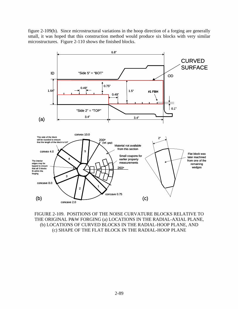
2-89

figure 2-109(b). Since microstructural variations in the hoop direction of a forging are generally small, it was hoped that this construction method would produce six blocks with very similar microstructures. Figure 2-110 shows the finished blocks.

FIGURE 2-109. POSITIONS OF THE NOISE CURVATURE BLOCKS RELATIVE TO THE ORIGINAL P&W FORGING (a) LOCATIONS IN THE RADIAL-AXIAL PLANE,

(b) LOCATIONS OF CURVED BLOCKS IN THE RADIAL-HOOP PLANE, AND (c) SHAPE OF THE FLAT BLOCK IN THE RADIAL-HOOP PLANE

260o

200o(ref. gap)

Material not availablefrom this section

This side of the blockwill be rounded to ensure that the length of the block is 6.8”

The interior edges may be lopped to ensure that all 5 blocks fit within the forging

concave 0.75

concave 2.0

concave 8.0

convex 4.0

convex 10.0

12

3

4

5Small coupons for earlier property measurements

Flat block was later machined from one of the

remaining wedges

2”

CURVEDSURFACE

1.64”0.75”

1.5”

6.8”

3.4”

0.49”

0.49”

3.4”

#1 FBH

0.1”

IDOD

“Side 5” = “BOT”

“Side 2” = “TOP”

(a)

(b) (c)

260o

200o(ref. gap)

Material not availablefrom this section

This side of the blockwill be rounded to ensure that the length of the block is 6.8”

The interior edges may be lopped to ensure that all 5 blocks fit within the forging

concave 0.75

concave 2.0

concave 8.0

convex 4.0

convex 10.0

12

3

4

5Small coupons for earlier property measurements

Flat block was later machined from one of the

remaining wedges

2”

CURVEDSURFACE

1.64”0.75”

1.5”

6.8”

3.4”

0.49”

0.49”

3.4”

#1 FBH

0.1”

IDOD

“Side 5” = “BOT”

“Side 2” = “TOP”

(a)

(b) (c)

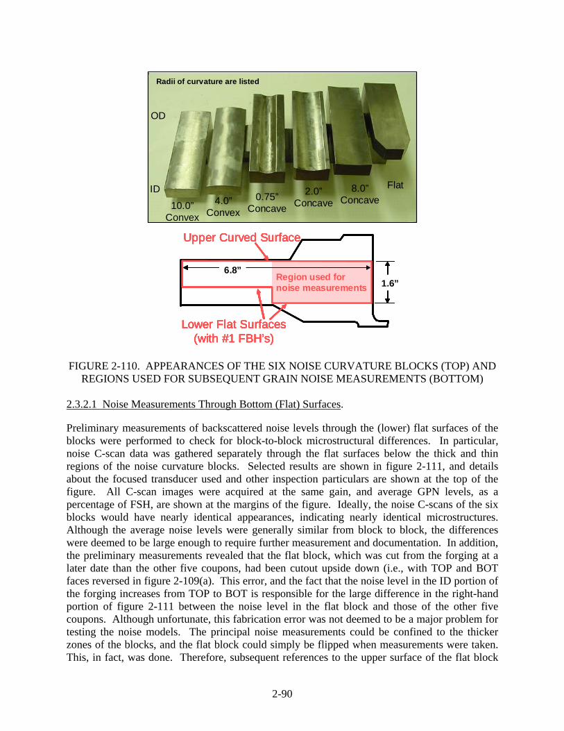
2-90

FIGURE 2-110. APPEARANCES OF THE SIX NOISE CURVATURE BLOCKS (TOP) AND

REGIONS USED FOR SUBSEQUENT GRAIN NOISE MEASUREMENTS (BOTTOM) 2.3.2.1 Noise Measurements Through Bottom (Flat) Surfaces.

Preliminary measurements of backscattered noise levels through the (lower) flat surfaces of the blocks were performed to check for block-to-block microstructural differences. In particular, noise C-scan data was gathered separately through the flat surfaces below the thick and thin regions of the noise curvature blocks. Selected results are shown in figure 2-111, and details about the focused transducer used and other inspection particulars are shown at the top of the figure. All C-scan images were acquired at the same gain, and average GPN levels, as a percentage of FSH, are shown at the margins of the figure. Ideally, the noise C-scans of the six blocks would have nearly identical appearances, indicating nearly identical microstructures. Although the average noise levels were generally similar from block to block, the differences were deemed to be large enough to require further measurement and documentation. In addition, the preliminary measurements revealed that the flat block, which was cut from the forging at a later date than the other five coupons, had been cutout upside down (i.e., with TOP and BOT faces reversed in figure 2-109(a). This error, and the fact that the noise level in the ID portion of the forging increases from TOP to BOT is responsible for the large difference in the right-hand portion of figure 2-111 between the noise level in the flat block and those of the other five coupons. Although unfortunate, this fabrication error was not deemed to be a major problem for testing the noise models. The principal noise measurements could be confined to the thicker zones of the blocks, and the flat block could simply be flipped when measurements were taken. This, in fact, was done. Therefore, subsequent references to the upper surface of the flat block

ID

OD

8.0”Concave

Flat2.0”Concave0.75”

Concave4.0”

Convex10.0”

Convex

Radii of curvature are listed

ID

OD

8.0”Concave

Flat2.0”Concave0.75”

Concave4.0”

Convex10.0”

Convex

Radii of curvature are listed

Upper Curved Surface

Lower Flat Surfaces(with #1 FBH’s)

Region used fornoise measurements

6.8”1.6”

Upper Curved Surface

Lower Flat Surfaces(with #1 FBH’s)

Region used fornoise measurements

Upper Curved Surface

Lower Flat Surfaces(with #1 FBH’s)

Region used fornoise measurements

6.8”1.6”

ID

OD

8.0”Concave

Flat2.0”Concave0.75”

Concave4.0”

Convex10.0”

Convex

Radii of curvature are listed

ID

OD

8.0”Concave

Flat2.0”Concave0.75”

Concave4.0”

Convex10.0”

Convex

Radii of curvature are listed

Upper Curved Surface

Lower Flat Surfaces(with #1 FBH’s)

Region used fornoise measurements

6.8”1.6”

Upper Curved Surface

Lower Flat Surfaces(with #1 FBH’s)

Region used fornoise measurements

Upper Curved Surface

Lower Flat Surfaces(with #1 FBH’s)

Region used fornoise measurements

6.8”1.6”

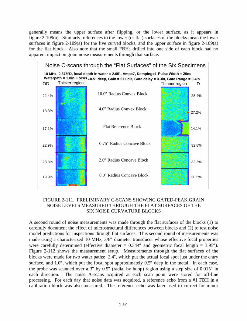
2-91

generally means the upper surface after flipping, or the lower surface, as it appears in figure 2-109(a). Similarly, references to the lower (or flat) surfaces of the blocks mean the lower surfaces in figure 2-109(a) for the five curved blocks, and the upper surface in figure 2-109(a) for the flat block. Also note that the small FBHs drilled into one side of each block had no apparent impact on grain noise measurements through that surface.

FIGURE 2-111. PRELIMINARY C-SCANS SHOWING GATED-PEAK GRAIN NOISE LEVELS MEASURED THROUGH THE FLAT SURFACES OF THE

SIX NOISE CURVATURE BLOCKS A second round of noise measurements was made through the flat surfaces of the blocks (1) to carefully document the effect of microstructural differences between blocks and (2) to test noise model predictions for inspections through flat surfaces. This second round of measurements was made using a characterized 10-MHz, 3/8″ diameter transducer whose effective focal properties were carefully determined (effective diameter = 0.344″ and geometric focal length = 3.95″). Figure 2-112 shows the measurement setup. Measurements through the flat surfaces of the blocks were made for two water paths: 2.4″, which put the actual focal spot just under the entry surface, and 1.0″, which put the focal spot approximately 0.5″ deep in the metal. In each case, the probe was scanned over a 3″ by 0.5″ (radial by hoop) region using a step size of 0.015″ in each direction. The noise A-scans acquired at each scan point were stored for off-line processing. For each day that noise data was acquired, a reference echo from a #1 FBH in a calibration block was also measured. The reference echo was later used to correct for minor

Thinner region

Noise C-scans through the “Flat Surfaces” of the Six Specimens

Thicker region

10 MHz, 0.375″D, focal depth in water = 2.65″, Amp=7, Damping=1,Pulse Width = 20ns Waterpath = 1.0in, Focus ≈0.5″ deep, Gain = 57.0dB, Gate delay = 0.3in, Gate Range = 0.4in

10.0″ Radius Convex Block

4.0″ Radius Convex Block

Flat Reference Block

0.75″ Radius Concave Block

2.0″ Radius Concave Block

8.0″ Radius Concave Block

OD ID

22.4%

18.8%

17.1%

22.9%

23.3%

19.9%

28.4%

14.1%

27.2%

32.8%

32.3%

30.5%

2-92

differences in measurement system efficiency from one measurement trial to the next. In addition, the electronic noise level was measured so that it could be properly accounted for when noise model predictions were compared with experiment.

FIGURE 2-112. EXPERIMENTAL SETUP FOR NOISE MEASUREMENTS USING THE NOISE CURVATURE BLOCKS

The types of grain noise data that were gathered are illustrated in figure 2-113. Raw noise A-scans were recorded and used to construct rms noise level curves and GPN C-scan images. The rms noise curves provided a convenient way of describing the manner in which the observed grain noise varies with depth. Their calculation from raw A-scan data is described in reference 29. Since no DAC was applied, the rms noise curves tend to peak near the focal zone, as is the case in figure 2-113(b). GPN C-scans are commonly used in industrial settings to describe the lateral variation of the noise. As illustrated in figure 2-113(c), GPN C-scans were constructed for four time gates (or depth zones), having the same center but different durations, as listed. As the time gate is enlarged, there are more opportunities to observed large grain noise amplitudes, and the measured GPN amplitude consequently tends to rise, as shown in the figure. For each GPN C-scan image, the average amplitude, the peak amplitude, and the standard deviation of the amplitudes about the mean were computed. The four inspection gates (G1-G4) whose centers and extents are indicated in figure 2-113(c) were consistently used for all noise measurements through both the flat and curved sides of the coupons.

scan

scan

Ti 6-4ForgingSpecimen

scanscan

scanscan

Ti 6-4ForgingSpecimen

#1 FBHin IN1100 reference

block

#1 FBHin IN1100 reference

block

Focused transducer had 3/8” diameter, 3.95” geom.

focal length in water.

2-93

Ring-down of front-wall echo

Back-wall echoGrain Noise

Typical RMS-Noise-Versus-Depth CurveFlat Block; Lower Surface; 1.0" Water Path

2

4

6

8

0.2 0.4 0.6 0.8 1 1.2 1.4 1.6

Depth (inches)

RMS

Noi

se L

evel

(%

FS

H) .

rmssmoothed

Zone 1

Zone 2

Zone 3

Zone 4

0.8”-1.0”

0.7”-1.1”

0.6”-1.2”

0.5”-1.3”

Zone location

OD ID

2.0” Concave Block; 1” Water Path; Flat Side

(G1)

(G2)

(G3)

(G4)

Zone 1

Zone 2

Zone 3

Zone 4

0.8”-1.0”

0.7”-1.1”

0.6”-1.2”

0.5”-1.3”

Zone location

OD ID

2.0” Concave Block; 1” Water Path; Flat Side

(G1)

(G2)

(G3)

(G4)

(a)

(b)

(c)

Ring-down of front-wall echo

Back-wall echoGrain Noise

Typical RMS-Noise-Versus-Depth CurveFlat Block; Lower Surface; 1.0" Water Path

2

4

6

8

0.2 0.4 0.6 0.8 1 1.2 1.4 1.6

Depth (inches)

RMS

Noi

se L

evel

(%

FS

H) .

rmssmoothed

Zone 1

Zone 2

Zone 3

Zone 4

0.8”-1.0”

0.7”-1.1”

0.6”-1.2”

0.5”-1.3”

Zone location

OD ID

2.0” Concave Block; 1” Water Path; Flat Side

(G1)

(G2)

(G3)

(G4)

Zone 1

Zone 2

Zone 3

Zone 4

0.8”-1.0”

0.7”-1.1”

0.6”-1.2”

0.5”-1.3”

Zone location

OD ID

2.0” Concave Block; 1” Water Path; Flat Side

(G1)

(G2)

(G3)

(G4)

(a)

(b)

(c)

FIGURE 2-113. EXAMPLES OF NOISE DATA (a) RAW NOISE A-SCAN AT ONE TRANSDUCER POSITION, (b) MEASURED AND SMOOTHED RMS NOISE-VERSUS-

DEPTH CURVES, AND (c) C-SCAN IMAGES FOR FOUR DEPTH ZONES

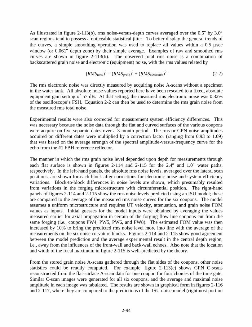
2-94

As illustrated in figure 2-113(b), rms noise-versus-depth curves averaged over the 0.5″ by 3.0″ scan regions tend to possess a noticeable statistical jitter. To better display the general trends of the curves, a simple smoothing operation was used to replace all values within a 0.5 μsec window (or 0.061″ depth zone) by their simple average. Examples of raw and smoothed rms curves are shown in figure 2-113(b). The observed total rms noise is a combination of backscattered grain noise and electronic (equipment) noise, with the rms values related by (RMStotal)2 = (RMSgrain)2 + (RMSelectronic)2 (2-2) The rms electronic noise was directly measured by acquiring noise A-scans without a specimen in the water tank. All absolute noise values reported here have been rescaled to a fixed, absolute equipment gain setting of 57 dB. At that setting, the measured rms electronic noise was 0.32% of the oscilloscope’s FSH. Equation 2-2 can then be used to determine the rms grain noise from the measured rms total noise. Experimental results were also corrected for measurement system efficiency differences. This was necessary because the noise data through the flat and curved surfaces of the various coupons were acquire on five separate dates over a 3-month period. The rms or GPN noise amplitudes acquired on different dates were multiplied by a correction factor (ranging from 0.93 to 1.09) that was based on the average strength of the spectral amplitude-versus-frequency curve for the echo from the #1 FBH reference reflector. The manner in which the rms grain noise level depended upon depth for measurements through each flat surface is shown in figures 2-114 and 2-115 for the 2.4″ and 1.0″ water paths, respectively. In the left-hand panels, the absolute rms noise levels, averaged over the lateral scan positions, are shown for each block after corrections for electronic noise and system efficiency variations. Block-to-block differences in noise levels are shown, which presumably resulted from variations in the forging microstructure with circumferential position. The right-hand panels of figures 2-114 and 2-115 show the rms noise levels predicted using an ISU model; these are compared to the average of the measured rms noise curves for the six coupons. The model assumes a uniform microstructure and requires UT velocity, attenuation, and grain noise FOM values as inputs. Initial guesses for the model inputs were obtained by averaging the values measured earlier for axial propagation in certain of the forging flow line coupons cut from the same forging (i.e., coupons PW4, PW5, PW6, and PW8). The estimated FOM value was then increased by 10% to bring the predicted rms noise level more into line with the average of the measurements on the six noise curvature blocks. Figures 2-114 and 2-115 show good agreement between the model prediction and the average experimental result in the central depth region, i.e., away from the influences of the front-wall and back-wall echoes. Also note that the location and width of the focal maximum in figure 2-115 is well-predicted by the theory. From the stored grain noise A-scans gathered through the flat sides of the coupons, other noise statistics could be readily computed. For example, figure 2-113(c) shows GPN C-scans reconstructed from the flat-surface A-scan data for one coupon for four choices of the time gate. Similar C-scan images were generated for all six coupons, and the average and maximal noise amplitude in each image was tabulated. The results are shown in graphical form in figures 2-116 and 2-117, where they are compared to the predictions of the ISU noise model (rightmost portion

2-95

of each plot). The model the does a good job of predicting the average GPN amplitude for each of the four gates. However, the theory tends to underestimate the maximum noise amplitude seen in a given C-scan. The noise model used in figures 2-116 and 2-117 again assumed a uniform average microstructure. The noise data indicate that the actual microstructure of a typical block varies only modestly with axial depth, but varies quite significantly with radial position, as shown in figure 2-113(c). Radial variations of noise FOM were incorporated into the noise model for later calculations.

FIGURE 2-114. COMPARISON OF MEASURED AND PREDICTED RMS GRAIN NOISE LEVELS FOR INSPECTIONS THROUGH THE FLAT SURFACES OF THE SIX NOISE

CURVATURE BLOCKS USING A 2.4″ WATER PATH

FIGURE 2-115. COMPARISON OF MEASURED AND PREDICTED RMS GRAIN NOISE LEVELS FOR INSPECTIONS THROUGH THE FLAT SURFACES OF THE SIX NOISE

CURVATURE BLOCKS USING A 1.0″ WATER PATH

Noise Measurements thru Flat Entry Surfaces2.4" water path; 57 dB

0

2

4

6

8

10

12

0.0 0.2 0.4 0.6 0.8 1.0 1.2 1.4 1.6

Metal Depth (inches)

RM

S G

rain

Noi

se (%

of F

SH)

.

Flat, FBHs in back Flat, FBHs in front

0.75 cv 2.0 cv

8.0 cv 4.0 cx

10.0 cx Theory

Exp. values corrected for electronic noise and Ref signal differences

Model assumes: FOM = 1.1* (5.6E-4*freq^1.25) Atten = 5.7E-4*freq^1.8

Noise Measurements thru Flat Entry Surfaces2.4" water path; 57 dB

0

2

4

6

8

10

12

0.0 0.2 0.4 0.6 0.8 1.0 1.2 1.4 1.6

Metal Depth (inches)

RM

S G

rain

Noi

se (%

of F

SH)

.

Theory Exp. Ave.

Exp. values correctedfor electronic noise and Ref signal differences

Model assumes: FOM = 1.1* (5.6E-4*freq^1.25) Atten = 5.7E-4*freq^1.8

Noise Measurements thru Flat Entry Surfaces2.4" water path; 57 dB

0

2

4

6

8

10

12

0.0 0.2 0.4 0.6 0.8 1.0 1.2 1.4 1.6

Metal Depth (inches)

RM

S G

rain

Noi

se (%

of F

SH)

.

Flat, FBHs in back Flat, FBHs in front

0.75 cv 2.0 cv

8.0 cv 4.0 cx

10.0 cx Theory

Exp. values corrected for electronic noise and Ref signal differences

Model assumes: FOM = 1.1* (5.6E-4*freq^1.25) Atten = 5.7E-4*freq^1.8

Noise Measurements thru Flat Entry Surfaces2.4" water path; 57 dB

0

2

4

6

8

10

12

0.0 0.2 0.4 0.6 0.8 1.0 1.2 1.4 1.6

Metal Depth (inches)

RM

S G

rain

Noi

se (%

of F

SH)

.

Theory Exp. Ave.

Exp. values correctedfor electronic noise and Ref signal differences

Model assumes: FOM = 1.1* (5.6E-4*freq^1.25) Atten = 5.7E-4*freq^1.8

Noise Measurements thru Flat Entry Surfaces1.0" water path; 57 dB

0

2

4

6

8

10

12

14

0.0 0.2 0.4 0.6 0.8 1.0 1.2 1.4 1.6

Metal Depth (inches)

RM

S G

rain

Noi

se (%

of F

SH)

. Flat, FBHs in back Flat, FBHs in front

0.75 cv 2.0 cv

8.0 cv 4.0 cx

10.0 cx Theory

Exp. values correctedfor electronic noise

Model assumes: FOM = 1.1* (5.6E-4*freq^1.25) Atten = 5.7E-4*freq^1.8

Noise Measurements thru Flat Entry Surfaces1.0" water path; 57 dB

0

2

4

6

8

10

12

14

0.0 0.2 0.4 0.6 0.8 1.0 1.2 1.4 1.6

Metal Depth (inches)

RM

S G

rain

Noi

se (%

of F

SH)

.

Theory Exp. Ave.

Exp. values correctedfor electronic noise

Model assumes: FOM = 1.1* (5.6E-4*freq^1.25) Atten = 5.7E-4*freq^1.8

Noise Measurements thru Flat Entry Surfaces1.0" water path; 57 dB

0

2

4

6

8

10

12

14

0.0 0.2 0.4 0.6 0.8 1.0 1.2 1.4 1.6

Metal Depth (inches)

RM

S G

rain

Noi

se (%

of F

SH)

. Flat, FBHs in back Flat, FBHs in front

0.75 cv 2.0 cv

8.0 cv 4.0 cx

10.0 cx Theory

Exp. values correctedfor electronic noise

Model assumes: FOM = 1.1* (5.6E-4*freq^1.25) Atten = 5.7E-4*freq^1.8

Noise Measurements thru Flat Entry Surfaces1.0" water path; 57 dB

0

2

4

6

8

10

12

14

0.0 0.2 0.4 0.6 0.8 1.0 1.2 1.4 1.6

Metal Depth (inches)

RM

S G

rain

Noi

se (%

of F

SH)

.

Theory Exp. Ave.

Exp. values correctedfor electronic noise

Model assumes: FOM = 1.1* (5.6E-4*freq^1.25) Atten = 5.7E-4*freq^1.8

2-96

FIGURE 2-116. MEASURED AND PREDICTED AVERAGE AMPLITUDES IN GPN C-SCAN IMAGES

(Results are shown for the four choices of the time gate (or depth zone) for each inspection water path.)

2.3.2.2 Correcting for Microstructural Differences.

The average noise characteristics, as reflected by the rms noise-versus-depth curves in figures 2-114 and 2-115, are somewhat different for the different blocks, indicating that the microstructures of the specimens are not identical. The differences in these flat-surface rms curves were used to determine microstructure difference factors, which were later used to approximately correct rms noise values measured through the curved surfaces.

Noise Measurements from flat side, water path = 1" Average Gated Peak Noise, Gain = 57 dB, I3 probe

0

5

10

15

20

25

Flat with FBH in back

Flat with FBH in front

0.75"concave

2.0"concave

8.0"concave

4.0"convex

10.0"convex

THEORY

% F

SH

Gate1 Gate 2 Gate 3 Gate 4

Noise Measurements from flat side, water path = 2.4"Average Gated Peak Noise, Gain = 57 dB, I3 probe

0

5

10

15

20

25

Flat with FBH in back

Flat with FBH in front

0.75"concave

2.0"concave

8.0"concave

4.0" convex 10.0"convex

THEORY

% F

SH

Gate1 Gate 2 Gate 3 Gate 4

2-97

FIGURE 2-117. MEASURED AND PREDICTED MAXIMUM AMPLITUDES IN GPN C-SCAN IMAGES

(Results are shown for the four choices of the time gate (or depth zone) for each inspection water path.)

For each block, the following four-step procedure was used to determine the depth-dependent microstructure difference factor from the flat-surface rms noise data. 1. The measured rms noise-versus depth curve was adjusted to remove the (minor) effect of

electronic noise.

2. The six rms noise curves (one for each block) were averaged to determine the mean curve for the suite of coupons. This was done separately for each of the two inspection water paths (2.4″ and 1.0″).

3. The rms noise curve for a given coupon was divided by the mean curve to determine the fractional deviation from the mean at each metal depth. As shown in figure 2-118, these difference factors were found to be nearly identical for the two inspections at different water paths, indicating that they do indeed arise from microstructural variations.

Noise Measurements from flat side, water path = 1" Maximum Gated Peak Noise, Gain = 57 dB, I3 probe

0

20

40

60

80

Flat with FBH in back

Flat with FBH in front

0.75"concave

2.0"concave

8.0"concave

4.0"convex

10.0"convex

THEORY

% F

SH

Gate1 Gate 2 Gate 3 Gate 4

Noise Measurements from flat side, water path = 2.4" Maximum Gated Peak Noise, Gain = 57 dB, I3 probe

0

20

40

60

80

Flat with FBH in back

Flat with FBH in front

0.75"concave

2.0"concave

8.0"concave

4.0" convex 10.0"convex

THEORY

% F

SH

Gate1 Gate 2 Gate 3 Gate 4

2-98

4. The difference factors measured for a given block using the 2.4″ and 1.0″ water paths were then averaged. In subsequence analyses of grain noise measured through the curved surfaces of the blocks, these difference factors were used (with the distance scale inverted) to correct noise quantities for microstructural differences. The correction procedure was relatively straightforward. In brief, if a measurement through the lower (flat) surface of a given coupon found the noise amplitude at depth Z to be 10% lower than the average for all coupons, then the noise amplitude measured at depth T-Z from the curved side was adjusted upward by 10%, where T denotes the coupon thickness.

FIGURE 2-118. (a)-(b) MICROSTRUCTURE DIFFERENCE FACTORS, AS

FUNCTIONS OF DEPTH, MEASURED USING WATER PATHS OF 2.4″ AND 1.0″, RESPECTIVELY AND (c)-(d) A MORE DETAILED VIEW OF THE

MICROSTRUCTURE CORRECTION FACTORS FOR TWO OF THE BLOCKS Average GPN C-scan amplitudes could be corrected in much the same way. Figure 2-119 shows the average GPN amplitudes measured through the flat (bottom) sides of the specimens. If the microstructures of the six coupons were identical, each curve would be a horizontal straight line. There are systematic departures from this ideal state: for example the 8″ concave specimen always has lower than average amplitude for each time gate and water path. To obtain rough microstructure correction factors for GPN, the noise amplitude for a given coupon was compared to the average overall six coupons (for a given gate and water path) to obtain a difference factor.

RMS grain noise in Ti noise curvature blocks measured from flat side, water path = 2.4"Normalized by average over six coupons.

0.60

0.80

1.00

1.20

1.40

1.60

1.80

0.0 0.2 0.4 0.6 0.8 1.0 1.2 1.4 1.6

Depth (inches)

Cou

pon

Noi

se /

Ave

rage

flat with FBHs in back0.75 cv2.0 cv8.0 cv4.0 cx10.0 cx

(5 and 0.62 dB corrections to "flat")

RMS grain noise in Ti noise curvature blocks measured from flat side, water path = 1"

Normalized by average over six coupons.

0.60

0.80

1.00

1.20

1.40

1.60

1.80

0.0 0.2 0.4 0.6 0.8 1.0 1.2 1.4 1.6

Depth (inches)

Cou

pon

Noi

se /

Ave

rage

flat with FBHs in back0.75 cv2.0 cv8.0 cv4.0 cx10.0 cx

RMS grain noise in Ti noise curvature blocks m easured from flat side, norm alized by average over six coupons.

0.6

0.7

0.8

0.9

1.0

1.1

1.2

1.3

1.4

0.0 0.2 0.4 0.6 0.8 1.0 1.2 1.4 1.6

Depth (inches)

Cou

pon

Noi

se /

Ave

rage

.

4.0 cx- 1.0"4.0 cx - 2.4"4.0 cx - ave.

4.0” – Convex Specimen

RMS grain noise in Ti noise curvature blocks m easured from flat s ide, norm alized by average over six coupons.

0.6

0.7

0.8

0.9

1.0

1.1

1.2

1.3

1.4

0.0 0.2 0.4 0.6 0.8 1.0 1.2 1.4 1.6

Depth (inches)

Cou

pon

Noi

se /

Ave

rage

. 0.75 cv - 1.0"0.75 cv - 2.4"0.75 cv - ave.

0.75” – Concave Specimen

(a) (b)

(c) (d)

RMS grain noise in Ti noise curvature blocks measured from flat side, water path = 2.4"Normalized by average over six coupons.

0.60

0.80

1.00

1.20

1.40

1.60

1.80

0.0 0.2 0.4 0.6 0.8 1.0 1.2 1.4 1.6

Depth (inches)

Cou

pon

Noi

se /

Ave

rage

flat with FBHs in back0.75 cv2.0 cv8.0 cv4.0 cx10.0 cx

(5 and 0.62 dB corrections to "flat")

RMS grain noise in Ti noise curvature blocks measured from flat side, water path = 1"

Normalized by average over six coupons.

0.60

0.80

1.00

1.20

1.40

1.60

1.80

0.0 0.2 0.4 0.6 0.8 1.0 1.2 1.4 1.6

Depth (inches)

Cou

pon

Noi

se /

Ave

rage

flat with FBHs in back0.75 cv2.0 cv8.0 cv4.0 cx10.0 cx

RMS grain noise in Ti noise curvature blocks m easured from flat side, norm alized by average over six coupons.

0.6

0.7

0.8

0.9

1.0

1.1

1.2

1.3

1.4

0.0 0.2 0.4 0.6 0.8 1.0 1.2 1.4 1.6

Depth (inches)

Cou

pon

Noi

se /

Ave

rage

.

4.0 cx- 1.0"4.0 cx - 2.4"4.0 cx - ave.

4.0” – Convex Specimen

RMS grain noise in Ti noise curvature blocks m easured from flat s ide, norm alized by average over six coupons.

0.6

0.7

0.8

0.9

1.0

1.1

1.2

1.3

1.4

0.0 0.2 0.4 0.6 0.8 1.0 1.2 1.4 1.6

Depth (inches)

Cou

pon

Noi

se /

Ave

rage

. 0.75 cv - 1.0"0.75 cv - 2.4"0.75 cv - ave.

0.75” – Concave Specimen

(a) (b)

(c) (d)

2-99

These difference factors are then averaged over water path and time gate choices. The averaged results are listed at the top of each plot in figure 2-119. For example, the value of 0.926 for the 2″ concave specimen means that the GPN level in that coupon tends to be about 7% below the average for the suite of six coupons.

FIGURE 2-119. AVERAGE GPN AMPLITUDES SEEN IN C-SCANS THROUGH THE FLAT SIDES OF THE NOISE CURVATURE BLOCKS

For the flat-side data for the 2.4″ water path inspection, the effect of applying the simple microstructure correction procedure is shown in figure 2-120. All data for a given coupon is divided by a single correction factor (e.g., 0.926 for the 8″ concave specimen). After correction, the average GPN amplitude is less dependent on the choice of coupon, but some residual scatter remains.

FIGURE 2-120. AVERAGE GPN AMPLITUDES SEEN IN C-SCANS THROUGH THE FLAT SIDES OF THE NOISE CURVATURE BLOCKS AT A 2.4″ WATER

PATH, BEFORE (LEFT) AND AFTER (RIGHT) CORRECTION FOR MICROSTRUCTURAL DIFFERENCES BETWEEN THE BLOCKS

Flat Side Inspection; 1.0" w.p.Average GPN

0

5

10

15

20

25

0.75"concave

2.0"concave

8.0"concave

flat 10.0"convex

4.0"convex

Ave

rage

GPN

(% F

SH

)

G1G2G3G4

Flat Side Inspection; 2.4" w.p.Average GPN

0

2

4

6

8

10

12

14

0.75"concave

2.0"concave

8.0"concave

flat 10.0"convex

4.0"convex

Ave

rage

GPN

(% F

SH)

G1G2G3G4

Microstructure Difference Factors:0.969 1.136 0.926 0.992 1.046 0.931

Microstructure Difference Factors:0.969 1.136 0.926 0.992 1.046 0.931

Flat Side Inspection; 1.0" w.p.Average GPN

0

5

10

15

20

25

0.75"concave

2.0"concave

8.0"concave

flat 10.0"convex

4.0"convex

Ave

rage

GPN

(% F

SH

)

G1G2G3G4

Flat Side Inspection; 2.4" w.p.Average GPN

0

2

4

6

8

10

12

14

0.75"concave

2.0"concave

8.0"concave

flat 10.0"convex

4.0"convex

Ave

rage

GPN

(% F

SH)

G1G2G3G4

Microstructure Difference Factors:0.969 1.136 0.926 0.992 1.046 0.931

Microstructure Difference Factors:0.969 1.136 0.926 0.992 1.046 0.931

Flat Side Inspection; 2.4" w.p.Average GPN

0

2

4

6

8

10

12

14

0.75"concave

2.0"concave

8.0"concave

flat 10.0"convex

4.0"convex

Ave

rage

GP

N (%

FSH

)

G1G2G3G4

Corrected for microstructural differences

Flat Side Inspection; 2.4" w.p.Average GPN

0

2

4

6

8

10

12

14

0.75"concave

2.0"concave

8.0"concave

flat 10.0"convex

4.0"convex

Ave

rage

GP

N (%

FS

H)

G1G2G3G4

Microstructure Difference Factors:0.969 1.136 0.926 0.992 1.046 0.931

Flat Side Inspection; 2.4" w.p.Average GPN

0

2

4

6

8

10

12

14

0.75"concave

2.0"concave

8.0"concave

flat 10.0"convex

4.0"convex

Ave

rage

GP

N (%

FSH

)

G1G2G3G4

Corrected for microstructural differences

Flat Side Inspection; 2.4" w.p.Average GPN

0

2

4

6

8

10

12

14

0.75"concave

2.0"concave

8.0"concave

flat 10.0"convex

4.0"convex

Ave

rage

GP

N (%

FS

H)

G1G2G3G4

Microstructure Difference Factors:0.969 1.136 0.926 0.992 1.046 0.931

Flat Side Inspection; 2.4" w.p.Average GPN

0

2

4

6

8

10

12

14

0.75"concave

2.0"concave

8.0"concave

flat 10.0"convex

4.0"convex

Ave

rage

GP

N (%

FSH

)

G1G2G3G4

Corrected for microstructural differences

Flat Side Inspection; 2.4" w.p.Average GPN

0

2

4

6

8

10

12

14

0.75"concave

2.0"concave

8.0"concave

flat 10.0"convex

4.0"convex

Ave

rage

GP

N (%

FS

H)

G1G2G3G4

Microstructure Difference Factors:0.969 1.136 0.926 0.992 1.046 0.931

2-100

Similar corrections were applied to GPN data acquired through the curved surfaces of the coupons. After correcting the grain noise properties for the microstructural differences between coupons, the remaining differences in noise properties are presumable due to surface curvature effects alone. In addition to the coupon-to-coupon differences, which presumably arise from microstructural variations in the hoop direction of the forging, the microstructure of each coupon varies significantly with radial position. These radial variations can also be quantified using the C-scans through the flat sides. To do this, the 1.0″ water path case with the widest gate (Gate 4) was chosen since that combination leads to the highest average noise level. One such C-scan image is shown at top left of figure 2-121. A horizontal profile of the image is calculated, i.e., at each horizontal (radial) position the values for the vertical (hoop) row of pixels are averaged. The results are shown in the graph at the bottom of figure 2-121 for each coupon. Also shown (small circles) is the average profile for the suite of six coupons.

FIGURE 2-121. RADIAL PROFILES OF THE NOISE C-SCANS THROUGH THE FLAT SIDES OF THE NOISE CURVATURE BLOCKS

The averaged radial profile from figure 2-121 is shown again in figure 2-122, where it has now been normalized to have an average value of unity over the 3-inch-wide radial range shown in either figure. Also displayed is a fourth-order polynomial fit that summarizes the general trend of the data. This smooth variation of noise level with radial position will be assumed in certain model calculations.

GPN Amplitude ProfileFlat Sides; 1.0" Water Path; Gate 4

0

5

10

15

20

25

30

35

40

45

0.0 1.0 2.0 3.0Radial Position (inches)

Ave

. GP

N A

mpl

itude

(% F

SH) .

Flat0.75" concave2.0" concave8.0" concave4.0" convex10.0" convexAverage

8.0″ concave block, flat side; 1.0″ water path

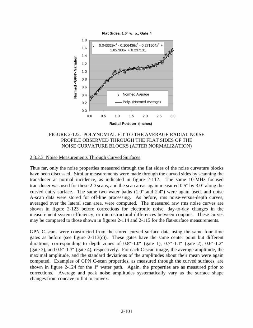
2-101

Flat Sides; 1.0" w. p.; Gate 4

y = 0.043329x4 - 0.106436x3 - 0.271504x2 + 1.057836x + 0.237131

0.0

0.2

0.4

0.6

0.8

1.0

1.2

1.4

1.6

1.8

0.0 0.5 1.0 1.5 2.0 2.5 3.0

Radial Position (inches)

Nor

med

<G

PN>

Varia

tion

Normed Average

Poly. (Normed Average)

FIGURE 2-122. POLYNOMIAL FIT TO THE AVERAGE RADIAL NOISE PROFILE OBSERVED THROUGH THE FLAT SIDES OF THE NOISE CURVATURE BLOCKS (AFTER NORMALIZATION)

2.3.2.3 Noise Measurements Through Curved Surfaces.

Thus far, only the noise properties measured through the flat sides of the noise curvature blocks have been discussed. Similar measurements were made through the curved sides by scanning the transducer at normal incidence, as indicated in figure 2-112. The same 10-MHz focused transducer was used for these 2D scans, and the scan areas again measured 0.5″ by 3.0″ along the curved entry surface. The same two water paths (1.0″ and 2.4″) were again used, and noise A-scan data were stored for off-line processing. As before, rms noise-versus-depth curves, averaged over the lateral scan area, were computed. The measured raw rms noise curves are shown in figure 2-123 before corrections for electronic noise, day-to-day changes in the measurement system efficiency, or microstructural differences between coupons. These curves may be compared to those shown in figures 2-114 and 2-115 for the flat-surface measurements. GPN C-scans were constructed from the stored curved surface data using the same four time gates as before (see figure 2-113(c)). These gates have the same center point but different durations, corresponding to depth zones of 0.8″-1.0″ (gate 1), 0.7″-1.1″ (gate 2), 0.6″-1.2″ (gate 3), and 0.5″-1.3″ (gate 4), respectively. For each C-scan image, the average amplitude, the maximal amplitude, and the standard deviations of the amplitudes about their mean were again computed. Examples of GPN C-scan properties, as measured through the curved surfaces, are shown in figure 2-124 for the 1″ water path. Again, the properties are as measured prior to corrections. Average and peak noise amplitudes systematically vary as the surface shape changes from concave to flat to convex.

2-102

Total RMS noise in Ti noise curvature blocks measured from curved side, water path = 1"

0

5

10

15

20

0.0 0.5 1.0 1.5 2.0

Depth, in

% o

f FSH

flat with FBHs in backflat with FBHs in front0.75 cv2.0 cv8.0 cv4.0 cx10.0 cx

Total RMS noise in Ti noise curvature blocks measured from curved side, water path = 2.4"

0

5

10

15

20

0.0 0.5 1.0 1.5 2.0

Depth, in

% o

f FSH

flat with FBHs in backflat with FBHs in front0.75 cv2.0 cv8.0 cv4.0 cx10.0 cx

Total RMS noise in Ti noise curvature blocks measured from curved side, water path = 1"

0

5

10

15

20

0.0 0.5 1.0 1.5 2.0

Depth, in

% o

f FSH

flat with FBHs in backflat with FBHs in front0.75 cv2.0 cv8.0 cv4.0 cx10.0 cx

Total RMS noise in Ti noise curvature blocks measured from curved side, water path = 2.4"

0

5

10

15

20

0.0 0.5 1.0 1.5 2.0

Depth, in

% o

f FSH

flat with FBHs in backflat with FBHs in front0.75 cv2.0 cv8.0 cv4.0 cx10.0 cx

FIGURE 2-123. RAW RMS NOISE-VERSUS-DEPTH CURVES AS MEASURED THROUGH THE CURVED SURFACES OF THE NOISE CURVATURE BLOCKS

The rms noise curves were corrected to remove the effect of electronic noise using equation 2-2. Both the rms noise curves and GPN amplitudes were corrected for measurement system efficiency difference, and for microstructural differences between the six coupons, in the manner described earlier in this section. In particular, for rms noise curves, the microstructure difference factors (as functions of depth) deduced from the flat-surface measurements (shown in figure 2-118) were used for the corrections, following the procedure on page 178. For GPN amplitudes, microstructural difference corrections were made in a similar way using the multiplicative factors shown in figure 2-120.

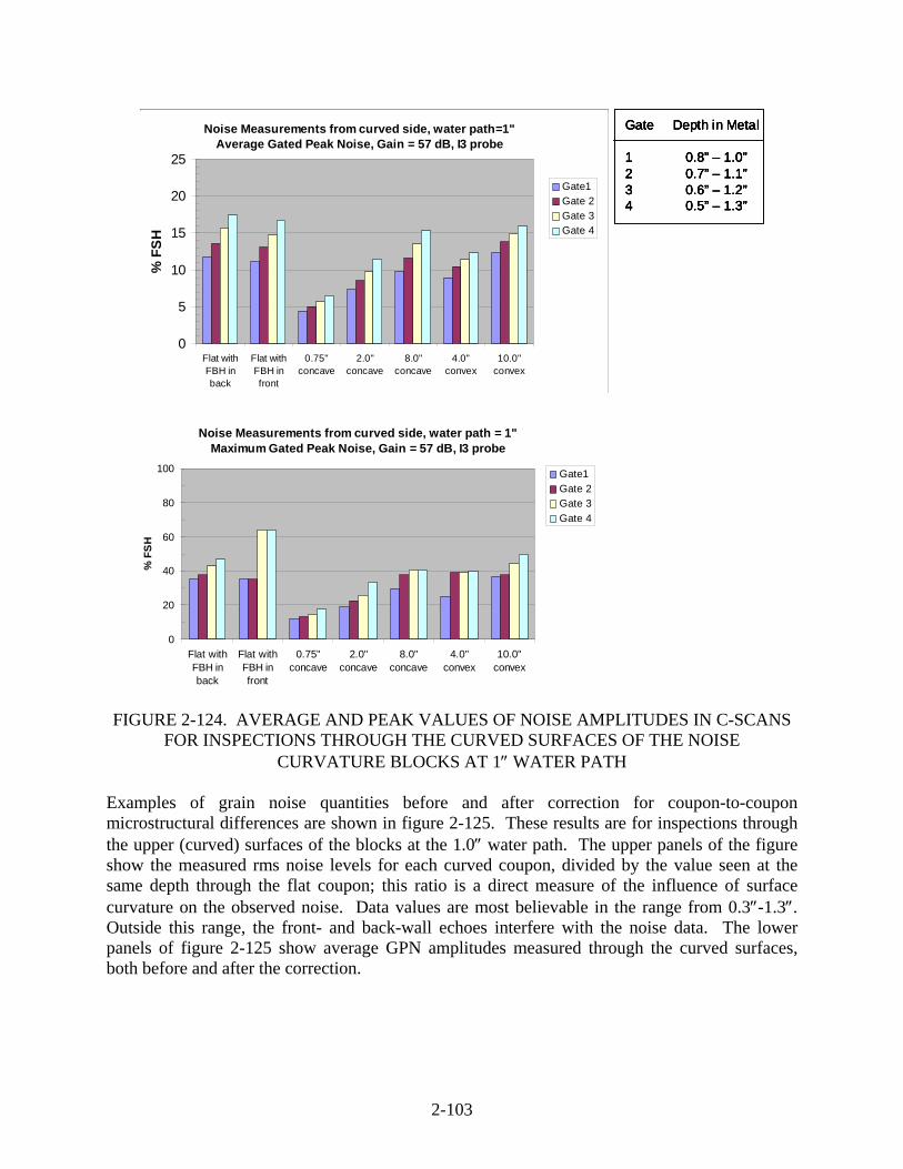
2-103

Noise Measurements from curved side, water path=1"Average Gated Peak Noise, Gain = 57 dB, I3 probe

0

5

10

15

20

25

Flat withFBH inback

Flat withFBH infront

0.75"concave

2.0"concave

8.0"concave

4.0"convex

10.0"convex

% F

SH

Gate1Gate 2Gate 3Gate 4

Noise Measurements from curved side, water path = 1"Maximum Gated Peak Noise, Gain = 57 dB, I3 probe

0

20

40

60

80

100

Flat withFBH inback

Flat withFBH infront

0.75"concave

2.0"concave

8.0"concave

4.0"convex

10.0"convex

% F

SH

Gate1Gate 2Gate 3Gate 4

Gate Depth in Metal

1 0.8” – 1.0”2 0.7” – 1.1”3 0.6” – 1.2”4 0.5” – 1.3”

Gate Depth in Metal

1 0.8” – 1.0”2 0.7” – 1.1”3 0.6” – 1.2”4 0.5” – 1.3”

Noise Measurements from curved side, water path=1"Average Gated Peak Noise, Gain = 57 dB, I3 probe

0

5

10

15

20

25

Flat withFBH inback

Flat withFBH infront

0.75"concave

2.0"concave

8.0"concave

4.0"convex

10.0"convex

% F

SH

Gate1Gate 2Gate 3Gate 4

Noise Measurements from curved side, water path = 1"Maximum Gated Peak Noise, Gain = 57 dB, I3 probe

0

20

40

60

80

100

Flat withFBH inback

Flat withFBH infront

0.75"concave

2.0"concave

8.0"concave

4.0"convex

10.0"convex

% F

SH

Gate1Gate 2Gate 3Gate 4

Gate Depth in Metal

1 0.8” – 1.0”2 0.7” – 1.1”3 0.6” – 1.2”4 0.5” – 1.3”

Gate Depth in Metal

1 0.8” – 1.0”2 0.7” – 1.1”3 0.6” – 1.2”4 0.5” – 1.3”

FIGURE 2-124. AVERAGE AND PEAK VALUES OF NOISE AMPLITUDES IN C-SCANS

FOR INSPECTIONS THROUGH THE CURVED SURFACES OF THE NOISE CURVATURE BLOCKS AT 1″ WATER PATH

Examples of grain noise quantities before and after correction for coupon-to-coupon microstructural differences are shown in figure 2-125. These results are for inspections through the upper (curved) surfaces of the blocks at the 1.0″ water path. The upper panels of the figure show the measured rms noise levels for each curved coupon, divided by the value seen at the same depth through the flat coupon; this ratio is a direct measure of the influence of surface curvature on the observed noise. Data values are most believable in the range from 0.3″-1.3″. Outside this range, the front- and back-wall echoes interfere with the noise data. The lower panels of figure 2-125 show average GPN amplitudes measured through the curved surfaces, both before and after the correction.

2-104

Curved Side Inspection; 1.0" w.p.Average GPN

0

2

4

6

8

10

12

14

16

18

20

0.75"concave

2.0"concave

8.0"concave

flat 10.0"convex

4.0"convex

Ave

rage

GP

N (%

FS

H)

G1G2G3G4

Curved Side Inspection; 1.0" w.p.Average GPN

0

2

4

6

8

10

12

14

16

18

20

0.75"concave

2.0"concave

8.0"concave

flat 10.0"convex

4.0"convex

Ave

rage

GP

N (%

FS

H)

G1G2G3G4

Corrected for microstructural differences

Effect of Curvature - 1.0" water path(Corrected for E-noise and system diffs)

0.2

0.4

0.6

0.8

1

1.2

1.4

1.6

0.0 0.2 0.4 0.6 0.8 1.0 1.2 1.4 1.6 1.8

Depth (inches)

RM

S N

oise

(fla

t = 1

)0.75 cv 2.0 cv8.0 cv 4.0 cx10.0 cx

RMS noise thru curve / RMS noise thru flat(not corrected for microstructural differences)

Effect of Curvature - 1.0" water path(Corrected for all other effects)

0.2

0.4

0.6

0.8

1

1.2

1.4

1.6

0.0 0.2 0.4 0.6 0.8 1.0 1.2 1.4 1.6 1.8

Depth (inches)

RM

S N

oise

(fla

t = 1

)

0.75 cv 2.0 cv8.0 cv 4.0 cx10.0 cx

RMS noise thru curve / RMS noise thru flat(corrected for microstructural differences)

1.0” water path 1.0” water path

Curved Side Inspection; 1.0" w.p.Average GPN

0

2

4

6

8

10

12

14

16

18

20

0.75"concave

2.0"concave

8.0"concave

flat 10.0"convex

4.0"convex

Ave

rage

GP

N (%

FS

H)

G1G2G3G4

Curved Side Inspection; 1.0" w.p.Average GPN

0

2

4

6

8

10

12

14

16

18

20

0.75"concave

2.0"concave

8.0"concave

flat 10.0"convex

4.0"convex

Ave

rage

GP

N (%

FS

H)

G1G2G3G4

Corrected for microstructural differences

Effect of Curvature - 1.0" water path(Corrected for E-noise and system diffs)

0.2

0.4

0.6

0.8

1

1.2

1.4

1.6

0.0 0.2 0.4 0.6 0.8 1.0 1.2 1.4 1.6 1.8

Depth (inches)

RM

S N

oise

(fla

t = 1

)0.75 cv 2.0 cv8.0 cv 4.0 cx10.0 cx

RMS noise thru curve / RMS noise thru flat(not corrected for microstructural differences)

Effect of Curvature - 1.0" water path(Corrected for all other effects)

0.2

0.4

0.6

0.8

1

1.2

1.4

1.6

0.0 0.2 0.4 0.6 0.8 1.0 1.2 1.4 1.6 1.8

Depth (inches)

RM

S N

oise

(fla

t = 1

)

0.75 cv 2.0 cv8.0 cv 4.0 cx10.0 cx

RMS noise thru curve / RMS noise thru flat(corrected for microstructural differences)

1.0” water path 1.0” water path

FIGURE 2-125. GRAIN NOISE ATTRIBUTES FOR MEASUREMENTS THROUGH THE UPPER (CURVED) SURFACES BEFORE (LEFT) AND AFTER (RIGHT) CORRECTIONS

FOR MICROSTRUCTURAL DIFFERENCES BETWEEN COUPONS 2.3.2.4 Noise Modeling.

Before displaying additional noise data for the curved surface measurements, the independent scatterer noise model whose predictions will be compared with experiment will be briefly discussed. The model assumes that the observed noise is an incoherent superposition of the direct echoes from the individual metal grains. Multiple scattering events are ignored. A flow chart for the model calculations is shown in figure 2-126. Reference 36 and the references cited therein describe the use of the basic model to predict the absolute rms noise level in a given inspection and the subsequent prediction of GPN amplitude distributions from rms noise-vs-time curves. The absolute noise level will depend on properties of the metal specimen and details of the inspection system. Metal UT properties that are input to the model include the density, sound speed, attenuation, and noise FOM. The latter is a frequency-dependent measure of the noise-generating capacity of the microstructure, equal to the square root of the standard backscatter power coefficient. The surface curvature changes the sound pattern injected into the component

2-105

by the transducer and, thus, determines which metal grains are insonified. This, in turn, impacts the backscattered noise characteristics. One step in the model calculations is the prediction of the incident sound pattern within the metal component. Examples of model calculations showing how the incident sound pattern is modified by surface curvature are shown in figure 2-127.

Average UT properties obtained from fundamental studies coupons(v, atten, FOM)

Measuredprobe focal characteristics (diameter, GFL)

UT system efficiency deduced from FBH reference signal

RMSNoiseModel

RMS grain noise level vs depth for average microstructure

Sonic pulse duration; Noise spatial correlation length

Empirical data on how noise varies with radial position

GatedPeakNoiseModel

Simulated noise C-scans; GPN statistics

Electronic noise level (measured)

Location and duration of time gate

Density = 4.43 gm/cm3

Velocity = 0.622 cm/usecAttenuation(f in MHz) =

0.00057 f 1.8 N/cmFOM(f in MHz) =

0.00062 f 1.25 cm –1/2

Average UT properties obtained from fundamental studies coupons(v, atten, FOM)

Measuredprobe focal characteristics (diameter, GFL)

UT system efficiency deduced from FBH reference signal

RMSNoiseModel

RMS grain noise level vs depth for average microstructure

Sonic pulse duration; Noise spatial correlation length

Empirical data on how noise varies with radial position

GatedPeakNoiseModel

Simulated noise C-scans; GPN statistics

Electronic noise level (measured)

Location and duration of time gate

Average UT properties obtained from fundamental studies coupons(v, atten, FOM)

Measuredprobe focal characteristics (diameter, GFL)

UT system efficiency deduced from FBH reference signal

RMSNoiseModel

RMSNoiseModel

RMS grain noise level vs depth for average microstructure

Sonic pulse duration; Noise spatial correlation length

Empirical data on how noise varies with radial position

GatedPeakNoiseModel

GatedPeakNoiseModel

Simulated noise C-scans; GPN statistics

Electronic noise level (measured)

Location and duration of time gate

Density = 4.43 gm/cm3

Velocity = 0.622 cm/usecAttenuation(f in MHz) =

0.00057 f 1.8 N/cmFOM(f in MHz) =

0.00062 f 1.25 cm –1/2

FIGURE 2-126. FLOW CHART FOR NOISE MODEL CALCULATIONS

1.5”

Thru 2” Concave Thru 4” ConvexThru Flat0.6”

1.5”

Thru 2” Concave Thru 4” ConvexThru Flat0.6”

1.5”

Thru 2” Concave Thru 4” ConvexThru Flat0.6”

FIGURE 2-127. PREDICTED INCIDENT ABSOLUTE PRESSURE AMPLITUDES AT 10 MHz WITHIN THREE OF THE NOISE CURVATURE BLOCKS FOR

THE TRANSDUCER USED IN THE EXPERIMENTS (A 1″ water path is assumed, and the upper surfaces are assumed to be curved

in the plane of the page.) The average UT properties (i.e., averaged over the 0.5″ by 3″ by 1.6″ scan volume) assumed in the model calculations were largely determined from prior measurements on four of the smaller forging flow line coupons and are listed in the upper left portion of figure 2-126. The standard

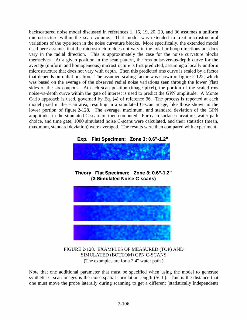
2-106

backscattered noise model discussed in references 1, 16, 19, 20, 29, and 36 assumes a uniform microstructure within the scan volume. That model was extended to treat microstructural variations of the type seen in the noise curvature blocks. More specifically, the extended model used here assumes that the microstructure does not vary in the axial or hoop directions but does vary in the radial direction. This is approximately the case for the noise curvature blocks themselves. At a given position in the scan pattern, the rms noise-versus-depth curve for the average (uniform and homogeneous) microstructure is first predicted, assuming a locally uniform microstructure that does not vary with depth. Then this predicted rms curve is scaled by a factor that depends on radial position. The assumed scaling factor was shown in figure 2-122, which was based on the average of the observed radial noise variations seen through the lower (flat) sides of the six coupons. At each scan position (image pixel), the portion of the scaled rms noise-vs-depth curve within the gate of interest is used to predict the GPN amplitude. A Monte Carlo approach is used, governed by Eq. (4) of reference 36. The process is repeated at each model pixel in the scan area, resulting in a simulated C-scan image, like those shown in the lower portion of figure 2-128. The average, maximum, and standard deviation of the GPN amplitudes in the simulated C-scan are then computed. For each surface curvature, water path choice, and time gate, 1000 simulated noise C-scans were calculated, and their statistics (mean, maximum, standard deviation) were averaged. The results were then compared with experiment.

Exp. Flat Specimen; Zone 3: 0.6”-1.2”

Theory Flat Specimen; Zone 3: 0.6”-1.2”(3 Simulated Noise C-scans)

Exp. Flat Specimen; Zone 3: 0.6”-1.2”

Theory Flat Specimen; Zone 3: 0.6”-1.2”(3 Simulated Noise C-scans)

FIGURE 2-128. EXAMPLES OF MEASURED (TOP) AND SIMULATED (BOTTOM) GPN C-SCANS

(The examples are for a 2.4″ water path.) Note that one additional parameter that must be specified when using the model to generate synthetic C-scan images is the noise spatial correlation length (SCL). This is the distance that one must move the probe laterally during scanning to get a different (statistically independent)

2-107

noise A-scan. Based on measurements at ISU using 10-MHz focused transducers and other Ti-6-4 forging specimens, an SCL value of 0.045″ was used in the model calculations. If a smaller SCL value is used (such as 0.015″, which equals the scan step size for noise measurements), then the speckle pattern in the simulated C-scan images is too fine when compared with experiment. This is demonstrated in figure 2-129.

One additional parameter which must be specified when using the model to generate synthetic C-scan images is the noise “spatial correlation length” (SCL). This is the distance that one must move the probe laterally to obtain a statistically independent noise A-scan. Based on measurements at ISU using 10-MHz focused transducers with other Ti 6-4 forging specimens, SCL= 0.045” has been used in our model calculations.

If a smaller SCL is used (say 0.015”), then the “speckle pattern” in the simulated C-scan images is too fine compared with experiment (top image), as shown at left.

Exp. Flat Specimen; Zone 3: 0.6”-1.2”

Theory Flat Specimen; Zone 3: 0.6”-1.2”(Simulated assuming SCL = 0.045” )

Theory Flat Specimen; Zone 3: 0.6”-1.2”(Simulated assuming SCL = 0.015” )

(Above examples are for 2.4” water path)

Role of the Noise Spatial CorrelationLength in Model Calculations

One additional parameter which must be specified when using the model to generate synthetic C-scan images is the noise “spatial correlation length” (SCL). This is the distance that one must move the probe laterally to obtain a statistically independent noise A-scan. Based on measurements at ISU using 10-MHz focused transducers with other Ti 6-4 forging specimens, SCL= 0.045” has been used in our model calculations.

If a smaller SCL is used (say 0.015”), then the “speckle pattern” in the simulated C-scan images is too fine compared with experiment (top image), as shown at left.

Exp. Flat Specimen; Zone 3: 0.6”-1.2”

Theory Flat Specimen; Zone 3: 0.6”-1.2”(Simulated assuming SCL = 0.045” )

Theory Flat Specimen; Zone 3: 0.6”-1.2”(Simulated assuming SCL = 0.015” )

(Above examples are for 2.4” water path)

Role of the Noise Spatial CorrelationLength in Model Calculations

FIGURE 2-129. ROLE OF THE NOISE SCL IN MODEL CALCULATIONS OF SYNTHETIC C-SCAN IMAGES

2.3.2.5 Effect of Surface Curvature on rms Noise Levels: Experiment and Theory.

Predicted rms noise-versus-depth curves, averaged over the 0.5″ by 3.0″ scan areas, are shown in figure 2-130 for each surface curvature and both inspection water paths. The two leftmost panels show the predicted absolute rms noise levels in the absence of electronic noise. One sees that the effect of a concave sound-entry surface curvature is to shorten the focal depth, thus enhancing the noise level at shallow depths and decreasing it deeper in the metal. The effect of convex curvature is just the opposite. The same trends are seen for both the 1.0″ and 2.4″ water paths, but the deviations from the flat-surface result are greater for the 1.0″ water path. The rightmost two panels of figure 2-130 show the predicted rms noise levels for each curved coupon divided by the predicted value at the same depth for the flat coupon. This dimensionless ratio is a direct measure of the influence of surface curvature on the observed noise level. Figure 2-131 compares measured and predicted rms noise-versus-depth curves normalized by the flat-surface result at the same depth. The measured values have been corrected to account for the day-to-day differences in the measurement system efficiency and for specimen-to-specimen microstructural differences. In addition, electronic noise was subtracted from the measured total noise to obtain an experimental measure of backscattered grain noise alone. Given the rather simple method used to correct for microstructural differences between specimens, the overall

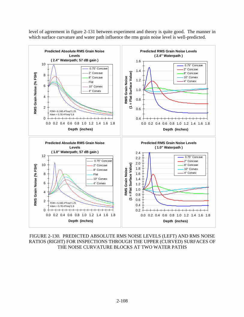
2-108

level of agreement in figure 2-131 between experiment and theory is quite good. The manner in which surface curvature and water path influence the rms grain noise level is well-predicted.

FIGURE 2-130. PREDICTED ABSOLUTE RMS NOISE LEVELS (LEFT) AND RMS NOISE RATIOS (RIGHT) FOR INSPECTIONS THROUGH THE UPPER (CURVED) SURFACES OF

THE NOISE CURVATURE BLOCKS AT TWO WATER PATHS

Predicted Absolute RMS Grain Noise Levels

( 2.4" Waterpath; 57 dB gain )

0

2

4

6

8

10

0.0 0.2 0.4 0.6 0.8 1.0 1.2 1.4 1.6 1.8

Depth (inches)

RM

S G

rain

Noi

se (%

FSH

) . 0.75" Concave

2" Concave8" ConcaveFlat10" Convex4" Convex

FOM = 6.16E-4*freq^1.25Atten = 5.7E-4*freq^1.8

Predicted RMS Grain Noise Levels( 2.4" Waterpath )

0.4

0.6

0.8

1.0

1.2

1.4

1.6

0.0 0.2 0.4 0.6 0.8 1.0 1.2 1.4 1.6 1.8

Depth (inches)R

MS

Gra

in N

oise

(1 =

Fla

t Sur

face

Val

ue)

0.75" Concave2" Concave8" Concave10" Convex4" Convex

Predicted Absolute RMS Grain Noise Levels

( 1.0" Waterpath; 57 dB gain )

0

2

4

6

8

10

12

0.0 0.2 0.4 0.6 0.8 1.0 1.2 1.4 1.6 1.8

Depth (inches)

RM

S G

rain

Noi

se (%

FSH

) . 0.75" Concave

2" Concave8" ConcaveFlat10" Convex4" Convex

FOM = 6.16E-4*freq^1.25Atten = 5.7E-4*freq^1.8

Predicted RMS Grain Noise Levels( 1.0" Waterpath )

0.20.40.60.81.01.21.41.61.82.02.22.4

0.0 0.2 0.4 0.6 0.8 1.0 1.2 1.4 1.6 1.8

Depth (inches)

RM

S G

rain

Noi

se(1

= F

lat S

urfa

ce V

alue

)

0.75" Concave2" Concave8" Concave10" Convex4" Convex

2-109

FIGURE 2-131. EFFECT OF SURFACE CURVATURE ON RMS NOISE-VERSUS-DEPTH

(Left: Experiment. Right: Model.) 2.3.2.6 Effect of Surface Curvature on GPN: Experiment and Theory.

Experimental and predicted values of GPN statistics in C-scan images are compared in figures 2-132 and 2-133 for inspections through the upper (curved) surfaces of the noise curvature blocks. The two figures show results for the 1.0″ and 2.4″ water paths, respectively. The upper panels of each figure display absolute average GPN amplitudes in %FSH units. The middle panels display the ratio of the standard deviation of the amplitudes to the average amplitude for each C-scan, and the lower panels display the ratio of the peak amplitude to the average amplitude. Again, experimental values were adjusted to correct for measurement system efficiency differences and for specimen-to-specimen microstructural differences. These adjustments do not alter the values of the experimental ratios shown in the figures, but do affect the absolute amplitudes shown in the upper panels. The model predictions were adjusted only to account for electronic noise. This was done by adding the measured rms electronic noise level to each predicted rms noise curve (using equation 2-2) before synthetic C-scans were generated.

Effect of Curvature - 2.4" water path(Corrected for all other effects)

0.4

0.6

0.8

1

1.2

1.4

0.0 0.2 0.4 0.6 0.8 1.0 1.2 1.4

Depth (inches)

RM

S N

oise

(fla

t = 1

)

0.75 cv 2.0 cv8.0 cv 4.0 cx10.0 cx

Predicted RMS Grain Noise Levels( 2.4" Waterpath )

0.4

0.6

0.8

1.0

1.2

1.4

0.0 0.2 0.4 0.6 0.8 1.0 1.2 1.4

Depth (inches)

RM

S G

rain

Noi

se(1

= F

lat S

urfa

ce V

alue

)

0.75" Concave2" Concave8" Concave10" Convex4" Convex

Effect of Curvature - 1.0" water path(Corrected for all other effects)

0.2

0.4

0.6

0.8

1

1.2

1.4

1.6

0.0 0.2 0.4 0.6 0.8 1.0 1.2 1.4

Depth (inches)

RM

S N

oise

(fla

t = 1

)

0.75 cv 2.0 cv8.0 cv 4.0 cx10.0 cx

Predicted RMS Grain Noise Levels( 2.4" Waterpath )

0.2

0.4

0.6

0.8

1.0

1.2

1.4

1.6

0.0 0.2 0.4 0.6 0.8 1.0 1.2 1.4

Depth (inches)

RM

S G

rain

Noi

se(1

= F

lat S

urfa

ce V

alue

) 0.75" Concave2" Concave8" Concave10" Convex4" Convex

(1.0” Water Path)

RMS noise thru curve / RMS noise thru flat(corrected for microstructural differences)

RMS noise thru curve / RMS noise thru flat(corrected for microstructural differences)

1.0” water path

2.4” water path

Effect of Curvature - 2.4" water path(Corrected for all other effects)

0.4

0.6

0.8

1

1.2

1.4

0.0 0.2 0.4 0.6 0.8 1.0 1.2 1.4

Depth (inches)

RM

S N

oise

(fla

t = 1

)

0.75 cv 2.0 cv8.0 cv 4.0 cx10.0 cx

Predicted RMS Grain Noise Levels( 2.4" Waterpath )

0.4

0.6

0.8

1.0

1.2

1.4

0.0 0.2 0.4 0.6 0.8 1.0 1.2 1.4

Depth (inches)

RM

S G

rain

Noi

se(1

= F

lat S

urfa

ce V

alue

)

0.75" Concave2" Concave8" Concave10" Convex4" Convex

Effect of Curvature - 1.0" water path(Corrected for all other effects)

0.2

0.4

0.6

0.8

1

1.2

1.4

1.6

0.0 0.2 0.4 0.6 0.8 1.0 1.2 1.4

Depth (inches)

RM

S N

oise

(fla

t = 1

)

0.75 cv 2.0 cv8.0 cv 4.0 cx10.0 cx

Predicted RMS Grain Noise Levels( 2.4" Waterpath )

0.2

0.4

0.6

0.8

1.0

1.2

1.4

1.6

0.0 0.2 0.4 0.6 0.8 1.0 1.2 1.4

Depth (inches)

RM

S G

rain

Noi

se(1

= F

lat S

urfa

ce V

alue

) 0.75" Concave2" Concave8" Concave10" Convex4" Convex

(1.0” Water Path)

RMS noise thru curve / RMS noise thru flat(corrected for microstructural differences)

RMS noise thru curve / RMS noise thru flat(corrected for microstructural differences)

Effect of Curvature - 2.4" water path(Corrected for all other effects)

0.4

0.6

0.8

1

1.2

1.4

0.0 0.2 0.4 0.6 0.8 1.0 1.2 1.4

Depth (inches)

RM

S N

oise

(fla

t = 1

)

0.75 cv 2.0 cv8.0 cv 4.0 cx10.0 cx

Predicted RMS Grain Noise Levels( 2.4" Waterpath )

0.4

0.6

0.8

1.0

1.2

1.4

0.0 0.2 0.4 0.6 0.8 1.0 1.2 1.4

Depth (inches)

RM

S G

rain

Noi

se(1

= F

lat S

urfa

ce V

alue

)

0.75" Concave2" Concave8" Concave10" Convex4" Convex

Effect of Curvature - 1.0" water path(Corrected for all other effects)

0.2

0.4

0.6

0.8

1

1.2

1.4

1.6

0.0 0.2 0.4 0.6 0.8 1.0 1.2 1.4

Depth (inches)

RM

S N

oise

(fla

t = 1

)

0.75 cv 2.0 cv8.0 cv 4.0 cx10.0 cx

Predicted RMS Grain Noise Levels( 2.4" Waterpath )

0.2

0.4

0.6

0.8

1.0

1.2

1.4

1.6

0.0 0.2 0.4 0.6 0.8 1.0 1.2 1.4

Depth (inches)

RM

S G

rain

Noi

se(1

= F

lat S

urfa

ce V

alue

) 0.75" Concave2" Concave8" Concave10" Convex4" Convex

(1.0” Water Path) Predicted RMS Grain Noise Levels

( 2.4" Waterpath )

0.2

0.4

0.6

0.8

1.0

1.2

1.4

1.6

0.0 0.2 0.4 0.6 0.8 1.0 1.2 1.4

Depth (inches)

RM

S G

rain

Noi

se(1

= F

lat S

urfa

ce V

alue

) 0.75" Concave2" Concave8" Concave10" Convex4" Convex

(1.0” Water Path)

RMS noise thru curve / RMS noise thru flat(corrected for microstructural differences)

RMS noise thru curve / RMS noise thru flat(corrected for microstructural differences)

1.0” water path

2.4” water path

2-110

Experiment Model

FIGURE 2-132. COMPARISON OF MEASURED (LEFT) AND PREDICTED (RIGHT) GPN

STATISTICS FOR NOISE C-SCANS MEASURED THROUGH THE UPPER (CURVED) SURFACES AT 1.0″ WATER PATH AND 57 dB GAIN

Curved Side Inspection; 1.0" w.p.Average GPN

0

2

4

6

8

10

12

14

16

18

20

0.75"concave

2.0"concave

8.0"concave

flat 10.0"convex

4.0"convex

Aver

age

GPN

(% F

SH)

G1G2G3G4

Corrected for microstructural differences

Curved Side Inspection; 1.0" w.p.Average GPN

0

2

4

6

8

10

12

14

16

18

20

0.75"concave

2.0"concave

8.0"concave

flat 10.0"convex

4.0"convex

Ave

rage

GP

N (%

FS

H)

G1G2G3G4

Curved Side Inspection; 1.0" w.p.Std. Deviation / Average of GPN

0.0

0.1

0.2

0.3

0.4

0.5

0.75"concave

2.0"concave

8.0"concave

flat 10.0"convex

4.0"convex

Std

. Dev

. / A

ve o

f GP

N

G1G2G3G4

Curved Side Inspection; 1.0" w.p.Std. Dev. / Ave GPN

0

0.1

0.2

0.3

0.4

0.5

0.75"concave

2.0"concave

8.0"concave

flat 10.0"convex

4.0"convex

Std

. Dev

. of G

PN

G1G2G3G4

Curved Side Inspection; 1.0" w.p.Maximum / Average GPN

0

1

2

3

4

5

0.75"concave

2.0"concave

8.0"concave

flat 10.0"convex

4.0"convex

Max

/ Ave

GP

N

G1G2G3G4

Curved Side Inspection; 1.0" w.p.Max / Ave GPN

0

1

2

3

4

5

0.75"concave

2.0"concave

8.0"concave

flat 10.0"convex

4.0"convex

Max

/ A

ve G

PN

G1G2G3G4

Curved Side Inspection; 1.0" w.p.Average GPN

0

2

4

6

8

10

12

14

16

18

20

0.75"concave

2.0"concave

8.0"concave

flat 10.0"convex

4.0"convex

Ave

rage

GP

N (%

FS

H)

G1G2G3G4

Corrected for microstructural differences

Curved Side Inspection; 1.0" w.p.Average GPN

0

2

4

6

8

10

12

14

16

18

20

0.75"concave

2.0"concave

8.0"concave

flat 10.0"convex

4.0"convex

Ave

rage

GP

N (%

FS

H)

G1G2G3G4

Curved Side Inspection; 1.0" w.p.Std. Deviation / Average of GPN

0.0

0.1

0.2

0.3

0.4

0.5

0.75"concave

2.0"concave

8.0"concave

flat 10.0"convex

4.0"convex

Std.

Dev

. / A

ve o

f GP

N

G1G2G3G4

Curved Side Inspection; 1.0" w.p.Std. Dev. / Ave GPN

0

0.1

0.2

0.3

0.4

0.5

0.75"concave

2.0"concave

8.0"concave

flat 10.0"convex

4.0"convex

Std

. Dev

. of G

PN

G1G2G3G4

Curved Side Inspection; 1.0" w.p.Maximum / Average GPN

0

1

2

3

4

5

0.75"concave

2.0"concave

8.0"concave

flat 10.0"convex

4.0"convex

Max

/ Ave

GP

N

G1G2G3G4

Curved Side Inspection; 1.0" w.p.Max / Ave GPN

0

1

2

3

4

5

0.75"concave

2.0"concave

8.0"concave

flat 10.0"convex

4.0"convex

Max

/ A

ve G

PN

G1G2G3G4

2-111

Experiment Model

FIGURE 2-133. COMPARISON OF MEASURED (LEFT) AND PREDICTED (RIGHT) GPN

STATISTICS FOR NOISE C-SCANS MEASURED THROUGH THE UPPER (CURVED) SURFACES AT 2.4″ WATER PATH AND 57 dB GAIN

Curved Side Inspection; 2.4" w.p.Average GPN

0

2

4

6

8

10

12

0.75"concave

2.0"concave

8.0"concave

flat 10.0"convex

4.0"convex

Ave

rage

GP

N (%

FS

H)

G1G2G3G4

Corrected for microstructural differences

Curved Side Inspection; 2.4" w.p.Average GPN

0

2

4

6

8

10

12

0.75"concave

2.0"concave

8.0"concave

flat 10.0"convex

4.0"convex

Ave

rage

GP

N (%

FS

H)

G1G2G3G4

Curved Side Inspection; 2.4" w.p.Std. Deviation / Average of GPN

0

0.1

0.2

0.3

0.4

0.5

0.75"concave

2.0"concave

8.0"concave

flat 10.0"convex

4.0"convex

Std

. Dev

. / A

ve o

f GPN

G1G2G3G4

Curved Side Inspection; 2.4" w.p.Std. Dev. / Ave GPN

0

0.1

0.2

0.3

0.4

0.5

0.75"concave

2.0"concave

8.0"concave

flat 10.0"convex

4.0"convex

Std.

Dev

. of G

PN

G1G2G3G4

Curved Side Inspection; 2.4" w.p.Maximum / Average GPN

0

1

2

3

4

5

0.75"concave

2.0"concave

8.0"concave

flat 10.0"convex

4.0"convex

Max

/ A

ve G

PN

G1G2G3G4

Curved Side Inspection; 2.4" w.p.Max / Ave GPN

0

1

2

3

4

5

0.75"concave

2.0"concave

8.0"concave

flat 10.0"convex

4.0"convex

Max

/ A

ve G

PN

G1G2G3G4

Curved Side Inspection; 2.4" w.p.Average GPN

0

2

4

6

8

10

12

0.75"concave

2.0"concave

8.0"concave

flat 10.0"convex

4.0"convex

Ave

rage

GP

N (%

FS

H)

G1G2G3G4

Corrected for microstructural differences

Curved Side Inspection; 2.4" w.p.Average GPN

0

2

4

6

8

10

12

0.75"concave

2.0"concave

8.0"concave

flat 10.0"convex

4.0"convex

Ave

rage

GP

N (%

FS

H)

G1G2G3G4

Curved Side Inspection; 2.4" w.p.Std. Deviation / Average of GPN

0

0.1

0.2

0.3

0.4

0.5

0.75"concave

2.0"concave

8.0"concave

flat 10.0"convex

4.0"convex

Std

. Dev

. / A

ve o

f GP

N

G1G2G3G4

Curved Side Inspection; 2.4" w.p.Std. Dev. / Ave GPN

0

0.1

0.2

0.3

0.4

0.5

0.75"concave

2.0"concave

8.0"concave

flat 10.0"convex

4.0"convex

Std.

Dev

. of G

PN

G1G2G3G4

Curved Side Inspection; 2.4" w.p.Maximum / Average GPN

0

1

2

3

4

5

0.75"concave

2.0"concave

8.0"concave

flat 10.0"convex

4.0"convex

Max

/ A

ve G

PN

G1G2G3G4

Curved Side Inspection; 2.4" w.p.Max / Ave GPN

0

1

2

3

4

5

0.75"concave

2.0"concave

8.0"concave

flat 10.0"convex

4.0"convex

Max

/ A

ve G

PN

G1G2G3G4

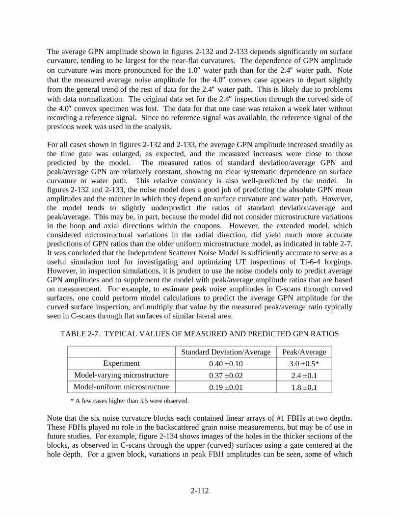
2-112

The average GPN amplitude shown in figures 2-132 and 2-133 depends significantly on surface curvature, tending to be largest for the near-flat curvatures. The dependence of GPN amplitude on curvature was more pronounced for the 1.0″ water path than for the 2.4″ water path. Note that the measured average noise amplitude for the 4.0″ convex case appears to depart slightly from the general trend of the rest of data for the 2.4″ water path. This is likely due to problems with data normalization. The original data set for the 2.4″ inspection through the curved side of the 4.0″ convex specimen was lost. The data for that one case was retaken a week later without recording a reference signal. Since no reference signal was available, the reference signal of the previous week was used in the analysis. For all cases shown in figures 2-132 and 2-133, the average GPN amplitude increased steadily as the time gate was enlarged, as expected, and the measured increases were close to those predicted by the model. The measured ratios of standard deviation/average GPN and peak/average GPN are relatively constant, showing no clear systematic dependence on surface curvature or water path. This relative constancy is also well-predicted by the model. In figures 2-132 and 2-133, the noise model does a good job of predicting the absolute GPN mean amplitudes and the manner in which they depend on surface curvature and water path. However, the model tends to slightly underpredict the ratios of standard deviation/average and peak/average. This may be, in part, because the model did not consider microstructure variations in the hoop and axial directions within the coupons. However, the extended model, which considered microstructural variations in the radial direction, did yield much more accurate predictions of GPN ratios than the older uniform microstructure model, as indicated in table 2-7. It was concluded that the Independent Scatterer Noise Model is sufficiently accurate to serve as a useful simulation tool for investigating and optimizing UT inspections of Ti-6-4 forgings. However, in inspection simulations, it is prudent to use the noise models only to predict average GPN amplitudes and to supplement the model with peak/average amplitude ratios that are based on measurement. For example, to estimate peak noise amplitudes in C-scans through curved surfaces, one could perform model calculations to predict the average GPN amplitude for the curved surface inspection, and multiply that value by the measured peak/average ratio typically seen in C-scans through flat surfaces of similar lateral area.

TABLE 2-7. TYPICAL VALUES OF MEASURED AND PREDICTED GPN RATIOS

Standard Deviation/Average Peak/Average Experiment 0.40 ±0.10 3.0 ±0.5*

Model-varying microstructure 0.37 ±0.02 2.4 ±0.1 Model-uniform microstructure 0.19 ±0.01 1.8 ±0.1

* A few cases higher than 3.5 were observed. Note that the six noise curvature blocks each contained linear arrays of #1 FBHs at two depths. These FBHs played no role in the backscattered grain noise measurements, but may be of use in future studies. For example, figure 2-134 shows images of the holes in the thicker sections of the blocks, as observed in C-scans through the upper (curved) surfaces using a gate centered at the hole depth. For a given block, variations in peak FBH amplitudes can be seen, some of which

2-113

are systematic (due to systematic attenuation variations with radial position) and some of which appear to be random. Such variations can be important when assessing detection reliability.

FIGURE 2-134. C-SCANS THROUGH THE UPPER (CURVED) SURFACES OF THE NOISE CURVATURE BLOCKS, SHOWING THE FBHs AT 1.5″ DEPTH

(The inspection water path was 1.0″.) Additional information about the noise curvature blocks and their use in testing backscattered noise models can be found in an article written for the Proceedings of the 2002 Conference on Quantitative NDE [37]. 2.3.3 Summary.

Some sound-entry surfaces for forging inspections are curved, which cause sound beams radiating into the forging to be altered. The sound beam will generally focus at a different depth and have different cross-sectional profiles compared to an inspection through a flat surface with the same transducer. Since the sound field impinging upon both defects and neighboring metal grains is altered, both defect signal amplitudes and backscattered grain noise levels will be changed. To study these changes, two sets of blocks were fabricated. The first set, known as the curvature correction blocks, were made from an ultrasonically neutral material (powder Ni alloy R88DT) and were used to study the effect of surface curvature on defect (FBH) echoes in the near absence of backscattered noise. The second set, known as the noise curvature blocks, were cut from a representative Ti-6-4 forging and were used to study the effect of surface curvature on backscattered grain noise characteristics. Each set consisted of six blocks, with each block having a different cylindrical curvature on the upper (sound-entry) surface. Three of the blocks in each set had concave radii of curvature (0.75″, 2.0″, and 8.0″); two had convex radii (4.0″ and 10.0″); and one block had a flat upper surface.

10” convex

4” convex

8” concave

2” concave

flat

10” convex

4” convex

8” concave

2” concave

flat

2-114

The curvature correction blocks each contained 13 #1 FBH reflectors, located at depths ranging from 0.5″ to 2.0″ beneath the upper (curved) surface. A series of experiments were performed in which 10-MHz transducers were scanned over the upper surfaces of the blocks and the peak amplitude of each FBH were measured. Three transducers were used, each with a fixed water path. Two of the transducers were I3 probes (nominally 10 MHz, 3/8″ diameter, 3″ focus) of the kind typically used for near-zone forging inspections. The third transducer, denoted as F10 (nominally 10 MHz, 1″ diameter, 10″ focus), was of the kind typically used for deeper-zone inspections. Each transducer was characterized to determine its effective diameter and geometrical focal length, and its efficiency factor for the conversion of electrical energy to sound was also measured. By comparing peak FBH amplitudes for inspections through curved and flat surfaces, curvature correction values (in dB units) were determined. The curvature correction, which is a function of depth, is defined as the receiver gain that must be added to an inspection to compensate for the effect of surface curvature on FBH amplitudes. Curvature corrections over the 0.5″-2″ depth range studied ranged from about -2 to +22 dB for the three measurement trials. As expected, the curvature corrections tended to be largest for the surfaces having the most severe curvatures. Measured curvature corrections were compared to the predictions of the ISU models, with the largest discrepancy between model and experiment was about 2 dB for the cases studied. The research team agreed that the flaw signal model appeared sufficiently accurate to be useful for calculating curvature corrections in forging inspections. The six noise curvature blocks each measured approximately 1.6″ by 5.9″ by 2″ (axial by radial by hoop) and were fabricated from the same Ti-6-4 forging that was the source of the P&W forging flow line coupons. The upper surface of each block was cylindrically curved, and the lower surface contained two flat steps into which several #1 FBHs were drilled. The holes played no role in the grain noise measurements. Preliminary measurements revealed that the flat block from the set had been cut upside down from the forging. This presented no real difficulties since the flat block could simply be flipped over, and the noise measurements were confined to the 1.6″ thick regions of the blocks. For the noise curvature blocks, measurements of backscattered grain noise properties were performed using a well-characterized 10-MHz, 3/8″ diameter focused transducer of the type generally used by P&W in forging inspections to depths of a few inches. Two inspection water paths were used: 2.4″, which put the actual focal spot just under the entry surface, and 1.0″, which put the focal spot approximately 0.5″ deep in the metal. Raw noise A-scans were recorded and used to construct rms noise level curves and GPN C-scan images. The rms noise curves provide a convenient way of describing the manner in which the observed grain noise varies with depth, and GPN C-scans are commonly used in industrial settings to describe the lateral variation of the noise. GPN C-scans were constructed for four time gates (or depth zones) having the same center but different durations, and for each, the average amplitude, the peak amplitude, and the standard deviation of the amplitudes about the mean were computed. Noise measurements through the bottom (flat) surfaces indicated that the microstructures of the six noise curvature blocks were not identical to one another. The differences seen in the flat-surface measurements were used to determine microstructure difference factors, which were later used to approximately correct the rms and GPN noise values measured through the upper (curved) surfaces for block-to-block microstructural differences. In addition, the noise

2-115

measurements through the lower (flat) surfaces revealed that the microstructures of the blocks varied systematically with radial position. The measured backscattered noise properties were found to depend significantly on surface curvature, with the deviations from the flat-surface case generally being more pronounced for the 1.0″ water path than for the 2.4″ water path. The measured (and corrected) rms noise-versus-depth curves and GPN properties were then compared to the predictions of the ISU models. The models were generalized to treat nonuniform microstructure in one direction (radial in this case) and to output simulated noise C-scan images. The noise model was found to do a good job of predicting (1) absolute rms noise-versus-depth curves for flat surface inspections, (2) the changes to rms noise-versus-depth curves that result from surface curvature, and (3) the average GPN amplitude seen in a C-scan, and the manner in which it depends on surface curvature, water path, and the choice of time gate. Although the model did a good job of predicting average noise properties, it tended to slightly underpredict the ratios of standard deviation/average and peak/average for noise C-scans. The research team concluded that the noise model is sufficiently accurate to serve as a useful simulation tool for investigating and optimizing UT inspections of Ti-6-4 forgings. However, in inspection simulations, it is prudent to use the noise models only to predict average GPN amplitudes, and then to supplement the model with peak/average amplitude ratios that are based on measurement. 2.4 SYNTHETIC INCLUSION DISK.

The capability of UT equipment and procedures to detect flaws is determined by inspecting blocks of representative material in which holes and notches have been machined [38]. Typically, the blocks are rectangular or cylindrical, and the holes are located to inspect the length of the hole or its top surface, such that they represent open cracks. With improved capabilities of inspection and the value of detecting ever-smaller flaws, there is a need to validate inspection capabilities with realistic defects located at all orientations within a part. Additionally, while machined holes and notches can represent cracks, flaws such as hard alpha inclusions in Ti have small reflectances [39], and there is a need for standardized referees at smaller target signal amplitudes [40]. An effort was undertaken, as summarized in this section, to embed synthetic hard alpha inclusions into a production aeroengine disk at various locations, sizes, and orientations—so that the disk could be used to assess the inspection capabilities on a part that would be representative of current industrial needs. The finished product was termed the synthetic inclusion disk. 2.4.1 Approach.

The approach selected was to obtain a disk, slice it on a plane perpendicular to its rotational axis of symmetry, embed hard alpha seeds, electron beam weld the disk pieces together on their periphery, and HIP the disk together. This approach had been previously used to make small seeded blocks [41]. The desired final disk would then be machined to the shape prescribed for UT inspection (sonic shape). Since the forging would lose some thickness from the cutting step, the forging was obtained as-forged with no machining. In this way, machining to final shape and thickness would be done after HIP bonding. To minimize any warping during slicing, the forging would be stress-relief

2-116

annealed. The seed locations would be selected after a UT scan of the forging to determine variability in grain noise. 2.4.2 Results and Discussion.

2.4.2.1 Measurements of UT Noise in an As-Forged Disk.

The disk obtained was a production Ti-6-4 forging of the same general design as used for the GE forging flow line coupons. The disk shape was ideal since it would comprise a real forging geometry along with embedded, controlled reflectors. The directional, textured nature of the microstructure within the forging would permit measurements of how the UT beam interacted with microstructural features. Figure 2-135 shows the etched macrostructure of an as-forged disk of the design selected, with the sonic outline to be machined superimposed on the image. The forging flow lines are generally parallel to the as-forged surfaces and to the final sonic inspection shape, except for the bore where flow lines are perpendicular to the part surface.

FIGURE 2-135. ETCHED MACROSTRUCTURE OF AN AS-FORGED DISK OF

THE SELECTED DESIGN The forging was purchased from the supplier in the pre-heat-treated condition with the as-forged surface. Figure 2-136 shows the disk as-received. The disk was inspected using a 10-MHz, F8 transducer (i.e., one having a focal length eight times its diameter) following a standard production inspection procedure. C-scans obtained were used to identify high- and low-noise regions and to plan the number and placement of targets. C-scan data were acquired before and after a light skim cut. The forged shape included a solid center since the bore had not yet been machined away. The inspection surfaces were neither flat nor concentric, and the surface finish was rougher than normally specified for UT inspection. The inspection could not achieve 0.06″ near-surface resolution due to these limitations, and the signal gate was increased to 0.2″ depth to avoid false alarm signals due to the rough entry surface. The OD was too irregular to be inspected at all. While noise patterns were detectable, confidence in the accuracy of the data was low due to poor surface conditions.

Bore

Rim

AFT

FWD

ODID

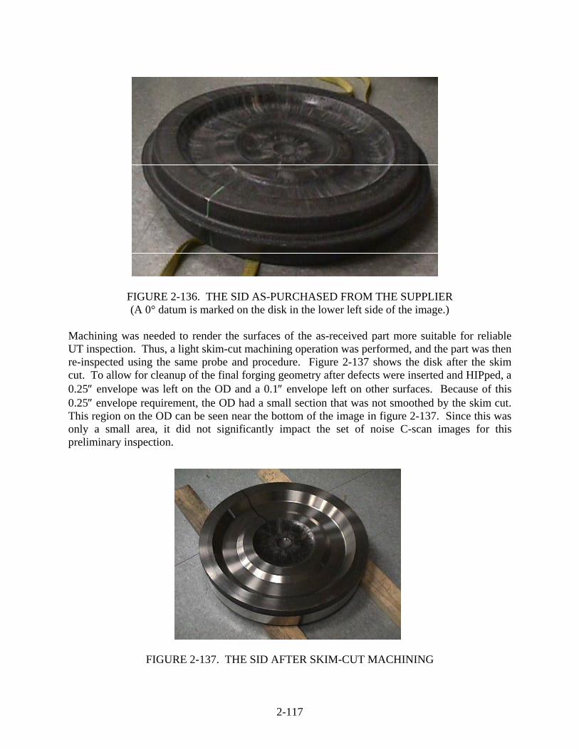
2-117

FIGURE 2-136. THE SID AS-PURCHASED FROM THE SUPPLIER (A 0° datum is marked on the disk in the lower left side of the image.)

Machining was needed to render the surfaces of the as-received part more suitable for reliable UT inspection. Thus, a light skim-cut machining operation was performed, and the part was then re-inspected using the same probe and procedure. Figure 2-137 shows the disk after the skim cut. To allow for cleanup of the final forging geometry after defects were inserted and HIPped, a 0.25″ envelope was left on the OD and a 0.1″ envelope left on other surfaces. Because of this 0.25″ envelope requirement, the OD had a small section that was not smoothed by the skim cut. This region on the OD can be seen near the bottom of the image in figure 2-137. Since this was only a small area, it did not significantly impact the set of noise C-scan images for this preliminary inspection.

FIGURE 2-137. THE SID AFTER SKIM-CUT MACHINING

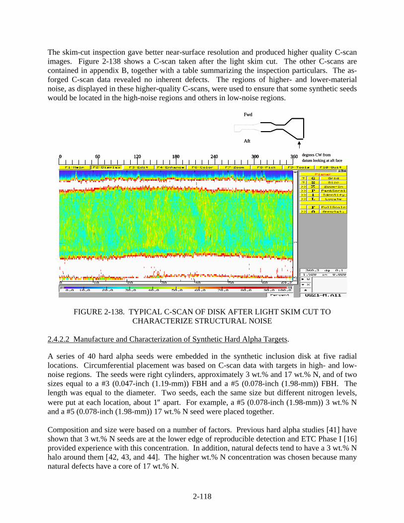
2-118

The skim-cut inspection gave better near-surface resolution and produced higher quality C-scan images. Figure 2-138 shows a C-scan taken after the light skim cut. The other C-scans are contained in appendix B, together with a table summarizing the inspection particulars. The as-forged C-scan data revealed no inherent defects. The regions of higher- and lower-material noise, as displayed in these higher-quality C-scans, were used to ensure that some synthetic seeds would be located in the high-noise regions and others in low-noise regions.

FIGURE 2-138. TYPICAL C-SCAN OF DISK AFTER LIGHT SKIM CUT TO

CHARACTERIZE STRUCTURAL NOISE

2.4.2.2 Manufacture and Characterization of Synthetic Hard Alpha Targets.

A series of 40 hard alpha seeds were embedded in the synthetic inclusion disk at five radial locations. Circumferential placement was based on C-scan data with targets in high- and low-noise regions. The seeds were right cylinders, approximately 3 wt.% and 17 wt.% N, and of two sizes equal to a #3 (0.047-inch (1.19-mm)) FBH and a #5 (0.078-inch (1.98-mm)) FBH. The length was equal to the diameter. Two seeds, each the same size but different nitrogen levels, were put at each location, about 1″ apart. For example, a #5 (0.078-inch (1.98-mm)) 3 wt.% N and a #5 (0.078-inch (1.98-mm)) 17 wt.% N seed were placed together. Composition and size were based on a number of factors. Previous hard alpha studies [41] have shown that 3 wt.% N seeds are at the lower edge of reproducible detection and ETC Phase I [16] provided experience with this concentration. In addition, natural defects tend to have a 3 wt.% N halo around them [42, 43, and 44]. The higher wt.% N concentration was chosen because many natural defects have a core of 17 wt.% N.

0 60 120 180 240 300 360

Fwd

Aft

degrees CW fromdatum looking at aft face

0 60 120 180 240 300 3600 60 120 180 240 300 360

Fwd

Aft

degrees CW fromdatum looking at aft face

2-119

Grain noise, arising from localized anisotropy of sound velocity within Ti-6-4 grains, was an additional consideration for selecting a low-nitrogen composition. It was desirable to select a low-nitrogen composition whose reflectance relative to a mean velocity in Ti-6-4 would be similar to maximum sound reflectance between maximally misaligned grains. Gigliotti [16] measured sound velocity in large Ti-6-4 grains: a maximum velocity of 6712 m/s was measured parallel to the c axis (hexagonal symmetry axis) orientation, and a minimum velocity of 6063 to m/s was measured perpendicular to the c-axis. This anisotropy could give rise to a 5% reflectance. In work measuring sound velocities of Ti-N alloys [39], a composition of 3 wt.% N was calculated to have about a 5% reflectance in host Ti-6-4 metal. A #1/2 (0.0078-inch (0.20-mm)) FBH presents 1/36 (or 2.8%) of the reflecting area of a #3 (0.047-inch (1.19-mm)) FBH. Therefore, an area-amplitude relationship would place the signal reflected by the #1/2 FBH target at 1/36 of the #3 FBH. However, the UT inspection of Ti disk forgings is typically conducted with 10-MHz, F8 transducers. Data sets acquired at 10 MHz on #1/2, #1, #2, and #3 FBHs show the signals reflected from the #1/2 FBH targets to fall within 3.7% and 4.3% of the #3 FBH. A theoretical explanation of this observation is still under development. Data acquired at 10 MHz on 0.047-inch (1.19-mm) -diameter, 3 wt.%N synthetic hard alpha inclusions also show reflectivities approximately 4% of a #3 FBH. It, therefore, seems reasonable to state that 3 wt.% N 0.047-inch (1.19-mm) synthetic hard alpha inclusions are expected to closely approximate a #1/2 FBH with respect to reflected signal amplitude, even though the two targets are a factor of 36 different in reflecting area. Table 2-8 gives the dimensions and measured sound velocities for all 40 synthetic hard alpha seeds that were placed in the disk. The #3 (0.047-inch (1.19-mm) seeds were too small to accurately measure shear velocities. With reference to table 2-9, the longitudinal velocity (cL) measurements were made using a 1/4″ diameter, 50-MHz transducer having a quartz buffer rod; the shear-wave velocities (cS) were measured with a 1/4″ diameter, 20-MHz quartz buffer rod transducer.

TABLE 2-8. SYNTHETIC HARD ALPHA SEED DIMENSIONS AND LONGITUDINAL- AND SHEAR-WAVE SOUND VELOCITIES

Seed No. wt.% N Length (mm)

Diameter (mm)

cL (mm/µs)

cS (mm/µs)

1 3 1.223 1.200 7.152 2 17 1.216 1.197 8.492 3 3 1.241 1.199 6.891 4 17 1.202 1.164 8.435 5 3 1.994 1.934 6.588 3.537 6 17 1.955 1.994 8.323 4.915 7 3 1.972 1.920 6.743 3.501 8 17 1.953 1.978 8.328 4.901 9 3 1.198 1.185 6.897 10 17 1.211 1.188 8.398 11 3 1.227 1.184 6.999 12 17 1.219 1.204 8.471

2-120

TABLE 2-8. SYNTHETIC HARD ALPHA SEED DIMENSIONS AND LONGITUDINAL- AND SHEAR-WAVE SOUND VELOCITIES (Continued)

Seed No. wt.% N Length (mm)

Diameter (mm)

cL (mm/µs)

cS (mm/µs)

13 3 1.982 1.911 6.678 3.576 14 17 1.923 1.986 8.314 4.918 15 3 1.995 1.939 6.619 3.542 16 17 1.962 1.965 8.307 4.908 17 3 1.251 1.207 6.923 18 17 1.209 1.192 8.562 19 3 1.192 1.185 6.819 20 17 1.250 1.223 8.735 21 3 1.982 1.929 6.653 3.628 22 17 1.966 1.963 8.306 4.894 23 3 2.021 1.985 6.551 3.513 24 17 1.999 1.975 8.336 4.885 25 3 1.211 1.227 6.881 26 17 1.218 1.169 8.559 27 3 1.198 1.188 6.768 28 17 1.299 1.190 9.339 29 3 1.983 1.925 6.645 3.632 30 17 1.956 1.954 8.295 4.921 31 3 2.002 1.910 6.638 3.539 32 17 1.961 1.951 8.309 4.896 33 3 1.231 1.210 7.010 34 17 1.208 1.166 8.513 35 3 1.236 1.213 7.112 36 17 1.243 1.177 8.456 37 3 2.003 1.950 6.619 3.351 38 17 1.979 1.968 8.368 4.905 39 3 2.011 1.938 6.570 3.505 40 17 1.930 1.974 8.308 4.917

Figure 2-139 shows a cumulative distribution probability plot for the seed velocities. This plot shows the velocities tightly bunched. The velocities of the #5 (0.078-inch (1.98-mm)) seeds are slightly lower than those of the #3 (0.047-inch (1.19-mm)) seeds. This is likely an artifact of the measurement process. The larger seeds were deburred after machining, while the smaller seeds were not. Since seed lengths were measured with a micrometer, the lengths of the smaller seeds may have a bias to positive error, since burr-to-burr length would be measured. 2.4.2.3 Incorporation of Synthetic Hard Alpha Within the Disk.

Using the C-scan images, regions of high- and low-grain noise below the flat inspection surfaces were identified in the forging. Figure 2-140 shows a schematic of the forging and the labeled scan surfaces, and figure 2-141 gives the forging dimensions. A single electron discharge

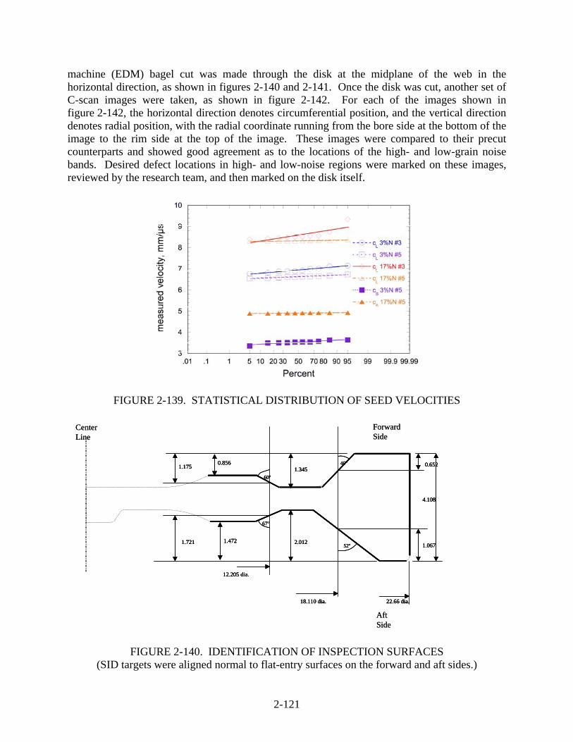
2-121

machine (EDM) bagel cut was made through the disk at the midplane of the web in the horizontal direction, as shown in figures 2-140 and 2-141. Once the disk was cut, another set of C-scan images were taken, as shown in figure 2-142. For each of the images shown in figure 2-142, the horizontal direction denotes circumferential position, and the vertical direction denotes radial position, with the radial coordinate running from the bore side at the bottom of the image to the rim side at the top of the image. These images were compared to their precut counterparts and showed good agreement as to the locations of the high- and low-grain noise bands. Desired defect locations in high- and low-noise regions were marked on these images, reviewed by the research team, and then marked on the disk itself.

FIGURE 2-139. STATISTICAL DISTRIBUTION OF SEED VELOCITIES

FIGURE 2-140. IDENTIFICATION OF INSPECTION SURFACES

(SID targets were aligned normal to flat-entry surfaces on the forward and aft sides.)

12.205 dia.

18.110 dia.

40°

52°

60°

67°

0.652

1.067

1.3451.175

2.0121.721 1.472

0.856

4.108

22.66 dia.

CenterLine

ForwardSide

AftSide

12.205 dia.

18.110 dia.

40°

52°

60°

67°

0.652

1.067

1.3451.175

2.0121.721 1.472

0.856

4.108

22.66 dia.

12.205 dia.

18.110 dia.

40°

52°

60°

67°

0.652

1.067

1.3451.175

2.0121.721 1.472

0.856

4.108

22.66 dia.

CenterLine

ForwardSide

AftSide

2-122

FIGURE 2-141. APPROXIMATE DIMENSIONS OF THE

SID IN ITS FINAL MACHINED FORM (The bold lines show machined surfaces, and the thin lines are

as-forged surfaces, which were removed in the final part.)

FIGURE 2-142. C-SCAN IMAGES (THROUGH SURFACES UH, UJ, UK, UL, AND UM)

OF THE SID AFTER EDM SLICING Holes for the #5 (0.078-inch (1.98-mm)) and #3 (0.047-inch (1.19-mm)) seeds were drilled on the internal surface, as shown in figure 2-143, in locations based on the C-scan images in figure 2-142. Figure 2-144 shows the full disk cross section with holes drilled. Three holes are marked for reference.

CenterLine

UM ULUK

UJ

UH

UG

US

UR

UPUO

Forward Side

Aft Side

CenterLine

UM ULUK

UJ

UH

UG

US

UR

UPUO

Forward Side

Aft Side

High noise Low noiseHigh noise Low noise

min max

0° 360°CCW direction

UH

UJ

UK

UL

UM

Inner Radius

Outer Radius

2-123

FIGURE 2-143. DRILLING SURFACE FOR SEED TARGETS

(Holes were drilled normal to the inspection surfaces along the internal side of the cut forging.)

FIGURE 2-144. AN SID WITH SEED HOLES DRILLED

(Three of the 40 total holes are marked.) For horizontal surfaces (e.g., UM at the bore), seeds normal to the forward side were also normal to the aft side (UO in this case). For sloped surfaces, half of the seeds were aligned normal to the forward surface (e.g., UL) and half were aligned normal to the aft surface (UP in this case). Normal seed alignment provides flat targets for area-amplitude calculations. Figure 2-145 schematically shows the location of all the seeds as viewed from the forward side of the SID. Figure 2-146 shows the seed locations viewed from the aft side, using the seed numbers in table 2-8. Figure 2-147 shows a seed being placed in the SID.

CenterLine

UM ULUK

UJ

UH

Drilled this surface

CenterLine

UM ULUK

UJ

UH

Drilled this surface

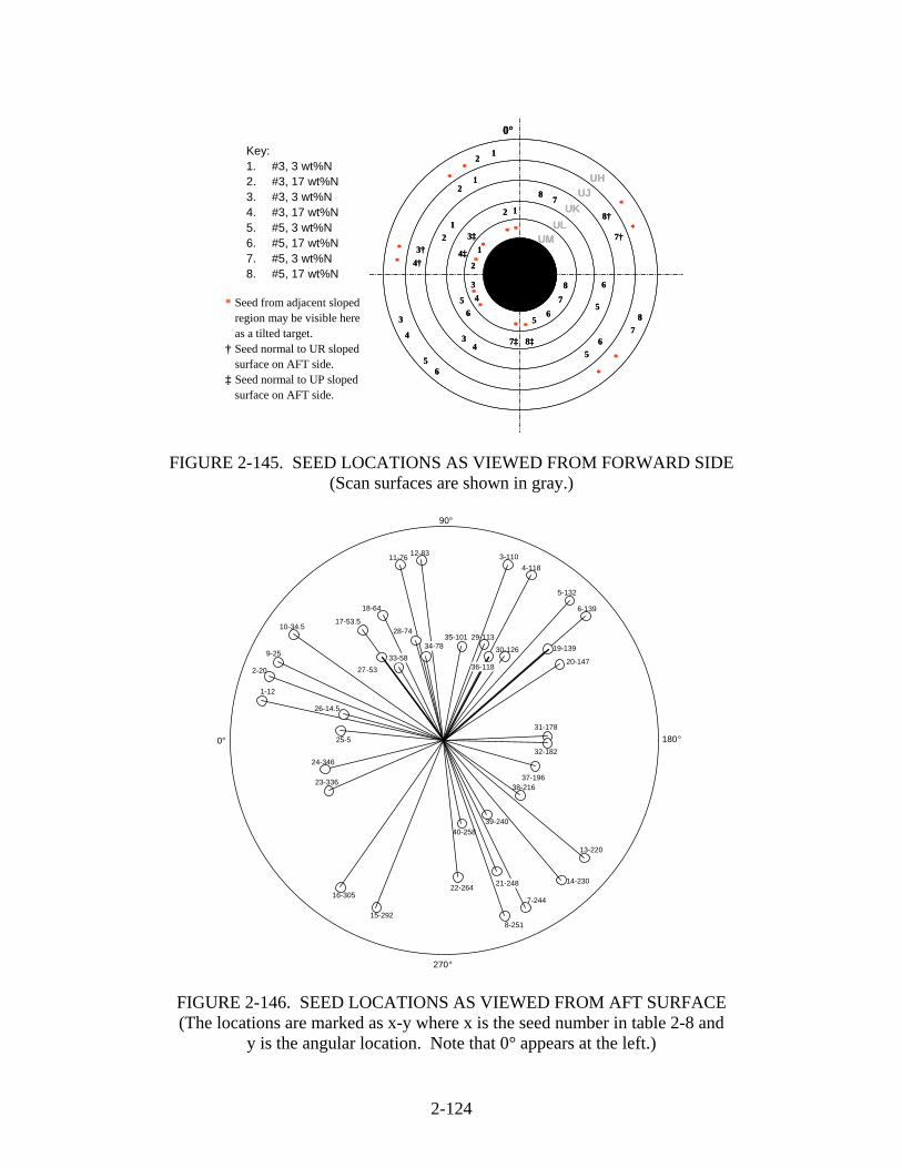
2-124

FIGURE 2-145. SEED LOCATIONS AS VIEWED FROM FORWARD SIDE (Scan surfaces are shown in gray.)

FIGURE 2-146. SEED LOCATIONS AS VIEWED FROM AFT SURFACE (The locations are marked as x-y where x is the seed number in table 2-8 and

y is the angular location. Note that 0° appears at the left.)

Key: 1. #3, 3 wt%N 2. #3, 17 wt%N 3. #3, 3 wt%N 4. #3, 17 wt%N 5. #5, 3 wt%N 6. #5, 17 wt%N 7. #5, 3 wt%N 8. #5, 17 wt%N

* Seed from adjacent sloped region may be visible here as a tilted target.

† Seed normal to UR sloped surface on AFT side.

‡ Seed normal to UP sloped surface on AFT side.

8‡

12

3

4

56

7 8

12

3†4†

56

7†

8†1

2

34

5

6

78

12

3‡

4‡

56

7‡

1

2

34

56

78

UH

0°

UJUK

ULUM

**

**

*

*

*

* ***

*

**

* *

8‡

12

3

4

56

7 8

12

3†4†

56

7†

8†1

2

34

5

6

78

12

3‡

4‡

56

7‡

1

2

34

56

78

UH

0°

UJUK

ULUM

**

**

*

*

*

* ***

*

**

* *

1-12

2-20

3-1104-118

5-132

6-139

7-244

0°

8-251

9-25

10-34.5

11-76 12-83

13-220

14-230

15-292

16-305

17-53.5

18-64

19-139

20-147

21-24822-264

23-336

25-5

26-14.5

27-53

28-7429-113

30-126

31-178

32-182

33-5834-78

35-101

36-118

37-19638-216

39-24040-258

90°

180°

270°

24-346

2-125

FIGURE 2-147. PLACEMENT OF AN SID SEED INTO AN EMPTY HOLE

(Another empty hole is visible at the lower left corner.) After the seeds were set in the disk, a prick-punch was used to wedge parent material around the hole to ensure the seeds would not fall out during handling. Figure 2-148 shows two seeds in the SID.

FIGURE 2-148. TWO SEEDS IN THE SID

(The prick-punch marks are the shiny spots at the upper left side of the seeds.)

After the seeds were placed, the two forging halves were welded together via electron beam welding, leak checked, and sent for HIPping. The initial HIP failed, which was caused by a leak in the bore of the disk. The location was identified, welded again, and the disk was sent out for a second HIP. This time the HIP succeeded. Figure 2-149 schematically illustrates the state of the disk at this point, with the approximate radial positions of the synthetic hard alpha seeds shown. Note that the seeds at radial locations 2 and 4 are shown tilted, to be normal to the aft surfaces. Only half of the seeds had that orientation. The other half (not shown) was tilted normal to the forward surfaces.

2-126

FIGURE 2-149. AN SID CROSS SECTION WITH EMBEDDED SEEDS

The disk was then machined to its final shape (see the white line in figure 2-149 and the dimensional values in figure 2-141). Another C-scan inspection was conducted to verify HIP quality and seed locations. No problems were found. 2.4.2.4 Machining of Flat Bottom Holes.

The final step in the SID fabrication was drilling the FBH targets. A total set of 18 FBHs were drilled in the three flat surfaces on the aft side. Three radial positions were used, as indicated in figure 2-150. Note that the FBHs were drilled in the opposite side of the disk from that used for drilling the small holes into which seeds were inserted. This design allows for inspection of certain FBHs through the large UL surface on the forward side rather than through the narrow US surface on the aft side.

FIGURE 2-150. AN SID CROSS SECTION SHOWING APPROXIMATE RADIAL

POSITIONS OF EMBEDDED SEEDS AND FBHs

Bore

Web

Rim

AFT

FWD

ODID

1 2* 3 4* 5

UO UPUR

US

UG

UJ

UH

UKULUM

Bore

Web

Rim

AFT

FWD

ODID

1 2* 3 4* 5

UO UPUR

US

UG

UJ

UH

UKULUM

Seed FBH

Bore

Web

Rim

AFT

FWD

ODID

1 2* 3 4* 5

UO UPUR

US

UG

UJ

UH

UKULUM

Seed FBH

Bore

Web

Rim

AFT

FWD

ODID

1 2* 3 4* 5

UO UPUR

US

UG

UJ

UH

UKULUM

Bore

Web

Rim

AFT

FWD

ODID

1 2* 3 4* 5

UO UPUR

US

UG

UJ

UH

UKULUM

2-127

Great care was taken when laying out the hole locations to ensure that none were put on top of a seed. At each radial location, one #5 (0.078-inch, 1.98-mm), one #3 (0.047-inch, 1.19-mm), and four #1 FBHs were drilled. For metal paths longer than a 10-to-1, length-to-diameter ratio, 1/4″ diameter counterbores were used. At the bottom of the counterbore, the actual FBH was drilled. The #3 and #5 FBHs permit true equivalent reflectivity measurements with seeds of the same size. These size holes traditionally have good reproducibility, thus, replicates at each location were not needed. The #1 FBHs serve as small targets for inspection, and replicates were placed at each location due to lower reproducibility. No #1/2 FBHs were drilled because they have poor reproducibility, and they cannot be drilled deep enough to ultrasonically resolve the hole from the backwall or the counterbore shoulder. Figure 2-151 shows the hole location map for the SID.

FIGURE 2-151. FLAT BOTTOM HOLE LOCATIONS, VIEWED FROM AFT SIDE

(Scan surfaces are labeled in gray.) Holes were drilled in surface US all at the same radial location 0.75″ in from the rim to an overall depth of 2.3875″. Holes drilled in surface UK were put at a location centered radially to an overall depth of 0.3755″. Holes drilled in surface UO were centered radially on the surface to an overall depth of 0.9155″. Figure 2-152 shows a composite view of the SID with both seed and FBH locations marked.

Key:A1 #5 FBH US, 50°B1 #3 FBH US, 65°C1 #1 FBH US, 340°C2 #1 FBH US, 270°C3 #1 FBH US, 200°C4 #1 FBH US, 160°

A2 #5 FBH UK, 320°B2 #3 FBH UK, 290°C5 #1 FBH UK, 305°C6 #1 FBH UK, 230°C7 #1 FBH UK, 110°C8 #1 FBH UK, 30°

A3 #5 FBH UO, 350°B3 #3 FBH UO, 335°C9 #1 FBH UO, 310°C10 #1 FBH UO, 290°C11 #1 FBH UO, 145°C12 #1 FBH UO, 30°

US

0°

URUK

UP

UO

A1

B1

C4C3

C2

C1

A2

C5

B2

C6

C7

C8

C12A3B3

C9

C10

C11

US

0°

URUK

UP

UO

A1

B1

C4C3

C2

C1

A2

C5

B2

C6

C7

C8

C12A3B3

C9

C10

C11

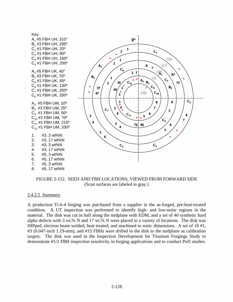
2-128

FIGURE 2-152. SEED AND FBH LOCATIONS, VIEWED FROM FORWARD SIDE

(Scan surfaces are labeled in gray.)

2.4.2.5 Summary.

A production Ti-6-4 forging was purchased from a supplier in the as-forged, pre-heat-treated condition. A UT inspection was performed to identify high- and low-noise regions in the material. The disk was cut in half along the midplane with EDM, and a set of 40 synthetic hard alpha defects with 3 wt.% N and 17 wt.% N were placed in a variety of locations. The disk was HIPped, electron beam welded, heat treated, and machined to sonic dimensions. A set of 18 #1, #3 (0.047-inch 1.19-mm), and #15 FBHs were drilled in the disk to the midplane as calibration targets. The disk was used in the Inspection Development for Titanium Forgings Study to demonstrate #1/2 FBH inspection sensitivity in forging applications and to conduct PoD studies.

Key:A1 #5 FBH UH, 310°B1 #3 FBH UH, 295ºC1 #1 FBH UH, 20ºC2 #1 FBH UH, 90ºC3 #1 FBH UH, 160ºC4 #1 FBH UH, 200º

A2 #5 FBH UK, 40°B2 #3 FBH UK, 70ºC5 #1 FBH UK, 55ºC6 #1 FBH UK, 130ºC7 #1 FBH UK, 250ºC8 #1 FBH UK, 330º

A3 #5 FBH UM, 10ºB3 #3 FBH UM, 25ºC9 #1 FBH UM, 50ºC10 #1 FBH UM, 70ºC11 #1 FBH UM, 215ºC12 #1 FBH UM, 330º

1. #3, 3 wt%N2. #3, 17 wt%N3. #3, 3 wt%N4. #3, 17 wt%N5. #5, 3 wt%N6. #5, 17 wt%N7. #5, 3 wt%N8. #5, 17 wt%N

8‡

12

3

4

56

78

12

3†4†

56

7†

8†1

2

34

5

6

78

12

3‡

4‡

56

7‡

1

2

34

56

7

8

UH

0°

UJUK

UL

UM

**

**

*

*

*

***

*

*

**

* *

A1

B1

C4 C3

C2

C1

A2

C5

B2

C6

C7

C8

C12A3 B3

C9

C10

C11

8‡

12

3

4

56

78

12

3†4†

56

7†

8†1

2

34

5

6

78

12

3‡

4‡

56

7‡

1

2

34

56

7

8

UH

0°

UJUK

UL

UM

**

**

*

*

*

***

*

*

**

* *

A1

B1

C4 C3

C2

C1

A2

C5

B2

C6

C7

C8

C12A3 B3

C9

C10

C11

3-1

3. SUMMARY.

The Engine Titanium Consortium (ETC) Phase II Fundamental Studies team was asked to investigate the fundamental ultrasonic (UT) properties of representative Ti-6-4 engine forgings, to explore the relationship of those properties to forging microstructure (e.g., flow line geometry), and to determine how those fundamental properties and forging surface curvatures impact inspectability. The team was also asked to use its data to suggest how forging inspections could be improved four-fold in amplitude (from #1 flat-bottom hole (FBH) detection sensitivity to #1/2 FBH sensitivity) and to make recommendations. The approach adopted by the team involved the fabrication and study of the four classes of test specimens listed in table 1-1. The first class of specimens, referred to as either the property measurement or forging flow line blocks, consisted of 26 small coupons, primarily rectangular prisms, which were cut from representative Ti-6-4 forged engine disks. Each of the three aircraft engine manufacturers (United Technologies Pratt & Whitney (P&W); General Electric Aircraft Engines (GE); and Honeywell Engines, Systems & Services) supplied one forging for this purpose, and the coupons were used to measure fundamental UT properties (velocity, attenuation, and backscattered grain noise). Most of the property measurement coupons were rectangular blocks, having one face perpendicular to the beam propagation direction for a standard normal incident longitudinal-wave disk inspection. However, one coupon from each disk was a cylinder used to better study the angular dependence of backscattered grain noise. Coupon locations in the axial-radial plane were chosen to span a wide range of microstructures, as revealed by flow line geometries (via macroetch) and forging strain patterns (via DEFORM™ calculations (a computer software program that is used to evaluate strain-to-cracking for hard alpha defects in typical billets and forgings)). In the hoop direction, coupons were cut from high-noise regions of the disks (as revealed by C-scans), since high-noise regions are generally the most difficult to inspect. Since the coupons were cut at various angles to the forging flow lines (or local macrograin orientation direction), the relationship between UT properties and the directionality of the local disk microstructure could be studied. All but three of the rectangular blocks were standard size, having nominal dimensions of 1.25″ by 1.25″ by 2.0″ (radial by axial by hoop). Systematic measurements on these blocks were performed to measure UT velocity, attenuation, and backscattered grain noise levels, and to subsequently investigate the relationship of the UT property variations to the flow line geometry. For all three forgings, sonic velocity variations measured over lengths of an inch or more were quite small, usually varying by less that 1 percent with position and inspection direction and, by themselves, are believed to pose no particular inspection difficulties. By contrast, variations of the UT attenuation and the average backscattered grain noise level with position and inspection direction in the radial-axial plane were quite large, with either quantity varying significantly within any given forging and varying by about an order of magnitude within the suite of forging flow line coupons. Measured attenuation values at 10 MHz ranged from 0.2 to 2.7 dB/inch, and maximal gated-peak noise (GPN) levels ranged from 0.5% to 6.9% of the amplitude of a #1 FBH reference reflector. The signal-to-noise (S/N) ratios quoted above are specifically for an inspection using a focused transducer having a particular sonic pulse volume (PV) (2.2E-5 cubic inches); noise-to-signal (N/S) ratios for other inspections can be estimated by using a rule of thumb that relates the N/S ratios to the square root of the PV.

3-2

Variations of noise and attenuation with position and inspection direction were found to be related to one another and to the details of the local forging strain. At a given location in a forging, the direction in which measured noise was greatest was generally the direction in which the measured attenuation was smallest. The maximal noise, minimal attenuation direction generally occurred for beam propagation perpendicular to the macrostructure elongation direction (i.e., the flow lines). The noise or attenuation anisotropy, defined as the value measured for axial propagation divided by that measured for radial propagation, calculated using DEFORM, was found to be well-correlated with the directionality of the local forging strain. More specifically, DEFORM calculations were performed in which circular or ellipsoidal volume elements in the billet (model macrograins) were tracked to determine their final shapes at the conclusion of the forging process. The noise or attenuation anisotropy was found to be well-correlated with the ratio of the projections of the forging macrograins onto the two inspection directions. The clear relationship between noise anisotropy and forging macrograin geometry led to the development of models that predict the variation of absolute grain noise levels within a forging. Two models were developed: a simpler one, which ignores metal texture, and a more complex one, which treats texture. The simpler model treats the forging as an effective scattering medium described by two global parameters that are the same at all points in the forging. One parameter describes the average size of the forging macrograins, and the other describes the average difference in elastic stiffness constants from one macrograin to the next. The model relies on DEFORM to calculate the shapes and orientations of the macrograins at various locations in the forging, assuming initial macrograins in the billet which are elongated in the axial direction. The simpler model assumes that crystalline axes within the macrograins are randomly oriented. The more complex version of the model takes into account the preferred orientations (texture) that develop in high strain regions. Both models were applied to predict noise variations throughout the P&W forging, and there was reasonable agreement with experiment. This suggests that noise variations within forgings can be largely understood from knowing the shapes and orientations of the elongated metal macrograins. Backscattered grain noise can mask the echo from a small or subtle defect in a forging, and, thus, plays a key role in determining defect detection limits. Although all the forging flow line coupons were cut from high-noise sections of the original equipment manufacturer-supplied forgings, some coupons had higher grain noise levels that others. Additional measurements were performed on the three coupons (one from each forging) with the largest absolute noise levels. The values of velocity, attenuation, and backscattered grain noise capacity (or figure of merit for noise severity) for these three worst-case microstructures were reported to the ETC, which were used as inputs to inspection simulation models that estimate the probability of defect detection for various forging inspection schemes. The three high-noise coupons were also used to determine beam focal requirements for achieving the #1/2 FBH detection sensitivity. As the sonic beam becomes better focused, the peak S/N ratio for a given defect tends to rise, being approximately proportional the reciprocal of the square root of the sonic PV at the defect’s location. The S/N ratios of the three high-noise coupons were repeatedly measured using different 10-MHz transducers and various water path choices to span a wide range of PVs. #1 FBH reflectors were drilled into the high-noise coupons to facilitate these measurements. Measured S/N ratios were in good agreement with the PV rule of thumb. The results indicated that a typical 10-MHz forging inspection that met the #1/2 FBH sensitivity target requires a beam diameter that does not exceed about 45 mils at any depth within a given inspection zone.

3-3

This information was used in a companion ETC study to design improved forging inspection schemes. The final use of the forging flow line coupons was to study UT signal fluctuations caused by the metal microstructure, such as the speckle that appears in back-wall amplitude C-scan images. Related fluctuations of FBH reference amplitudes or defect-signal amplitudes have important implications for probability of detection. To study the fluctuations, a small receiving transducer (pinducer) was used to map the amplitude and phase profiles of sonic beams that emerged after passing through titanium (Ti) alloy and fused-quartz blocks. It was shown that distortions of the beam profiles by the Ti microstructure were responsible for the variation in back-wall amplitude when the transmitting probe was scanned in pulse/echo mode. The beam profile maps were also used to measure the energy-loss attenuation in selected forging flow line coupons. For these coupons, the average attenuation value deduced from planar probe pulse/echo measurements of back-wall amplitude was generally close to the energy-loss value. Thus, the beam distortions caused the back-wall amplitude to be higher at some locations and lower at others, but on average, near that expected due to energy loss alone. Work was also begun to develop a model that could predict the back-wall signal fluctuation level from known model parameters, which described the nature and severity of the beam distortions, with those model parameters themselves measured via through-transmission, beam-mapping experiments. Initial tests of the model formalism, both experimentally and through computer simulations, appeared promising. The continued development and testing of signal fluctuation models, and their extension to small reflectors (e.g., FBHs), would be a useful avenue for future work. Some sound-entry surfaces for forging inspections are curved, and the curvature causes the interrogating sound beam to focus at a different depth and have different cross-sectional profiles compared to an inspection through a flat surface with the same transducer. Both defect signal amplitudes and backscattered grain noise levels are affected. To study these effects, two sets of blocks were fabricated. The first set, known as the curvature correction blocks, was made from an ultrasonically neutral material (powder nickel alloy R88DT) and was used to study the effect of surface curvature on defect (FBH) echoes in the near absence of backscattered noise. The second set, known as the noise curvature blocks, was cut from a representative Ti-6-4 forging and was used to study the effect of surface curvature on backscattered grain noise characteristics. Each set consisted of six blocks, with each block having a different cylindrical curvature on the upper (sound-entry) surface. Three of the blocks in each set had concave radii of curvature (0.75″, 2.0″, and 8.0″); two had convex radii (4.0″and 10.0″); and one block had a flat upper surface. The curvature correction blocks each contained 13 #1 FBH reflectors, located at depths ranging from 0.5″ to 2.0″ beneath the upper (curved) surface. A series of experiments were performed in which 10-MHz transducers were scanned over the upper surfaces of the blocks, and the peak amplitude of each FBH were measured. By comparing peak FBH amplitudes for inspections through curved and flat surfaces, depth-dependent curvature correction values were determined, defined as the receiver gain that must be added to an inspection to compensate for the effect of surface curvature on FBH amplitudes. Curvature corrections over the 0.5″-2″ depth range studied ranged from about -2 to +22 dB for the three measurement trials using different transducers. As expected, the curvature corrections tended to be largest for the surfaces having

3-4

the most severe curvatures. Measured curvature corrections were compared to the predictions of the Iowa State University (ISU) models, and the largest discrepancy between model and experiment was about 2 dB for the cases studied. The research team agreed that the flaw signal model appeared sufficiently accurate to be useful for calculating curvature corrections in forging inspections. The six noise curvature blocks were fabricated from the same Ti-6-4 forging, which was the source of the P&W forging flow line coupons. The upper surface of each block was cylindrically curved, and the lower surfaces were flat. Measurements of backscattered grain noise properties were performed through both the flat and curved surfaces using a 10-MHz focused transducer often used in forging inspections to depths of a few inches. Two inspection water paths were used to investigate two different focal conditions. Raw noise A-scans were recorded and used to construct root mean squared (rms) noise level curves and GPN C-scan images. The rms noise curves provided a convenient way of describing the manner in which the observed grain noise varies with depth, and GPN C-scans are commonly used in industrial settings to describe the lateral variation of the noise. GPN C-scans were constructed for four time gates (or depth zones) having the same center but different durations, and for each, the average amplitude, the peak amplitude, and the standard deviation of the amplitudes about the mean were computed. Measurements through the bottom (flat) surfaces of the noise curvature blocks were used to document block-to-block microstructural differences and to determine appropriate correction factors. Noise measurements through the upper (curved) surfaces were then corrected for microstructural differences to isolate the effects due to curvature alone. The effect of surface curvature on the measured noise was quite significant, with absolute noise levels altered by up to a factor of 3 compared to the flat-surface case. The measured rms noise-versus-depth curves and GPN properties were compared to the predictions of the ISU models. The noise models were generalized to (1) treat nonuniform microstructures and (2) output simulated noise C-scan images. The noise model did a good job of predicting (1) absolute rms noise-versus-depth curves for flat surface inspections; (2) the changes to rms noise-versus-depth curves that result from surface curvature; and (3) the average GPN amplitude in a C-scan, and the manner in which it depends on surface curvature, water path, and the choice of time gate. Although the model did a good job of predicting average noise properties, it tended to slightly underpredict the ratios of standard deviation/average and peak/average for noise C-scans. The team concluded that the noise model was sufficiently accurate to serve as a useful simulation tool for investigating and optimizing UT inspections of Ti-6-4 forgings. However, in C-scan simulations, it was prudent to use the noise models only to predict average GPN amplitudes, and then to supplement the model with peak/average amplitude ratios that are based on direct measurement. The final specimen fabricated by the Fundamental Studies task group was the synthetic inclusion disk (SID). This was constructed by taking a representative Ti-6-4 forged disk, slicing it in a plane perpendicular to the axis of rotational symmetry, inserting artificial defects, and then HIPping the two halves of the disk back together. The basic disk geometry was the same as the GE-supplied forging flow line coupons. The seeded internal defects were 40 synthetic hard alpha inclusions. These were right circular cylinders of two sizes (#3 and #5 diameters and

3-5/3-6

lengths) and two nitrogen impurity levels (3% and 17% nitrogen by weight). The two impurity levels are typical of those in the halo and core regions, respectively, of real hard alpha defects. The inclusions with the smaller diameter and smaller impurity level were expected to produce UT echoes of similar amplitude to #1/2 FBHs. The inclusions were placed into a variety of locations, some having high-grain noise levels and some having low-grain noise levels, as identified by UT C-scans prior to slicing. After assembly and HIPping were successfully accomplished, 18 FBHs were drilled into the SID to serve as additional reference reflectors. These were of three sizes: #1 (12 holes), #3 (3 holes), and #5 (3 holes). After fabrication, the SID was forwarded to another ETC Phase II team for use in assessing various inspection methods aimed at achieving #1/2 FBH detection sensitivity. The research activities summarized in this report were the basis for seven scientific papers written for the open literature, namely, references 23, 24, 25, 33, 34, 35, and 38. The ETC specimens fabricated during this research program are listed in appendix C.

4-1

4. REFERENCES.

1. Margetan, F.J., Han, K.Y., Yalda, I., Goettsch, S., and Thompson, R.B., “The Practical Application of Grain Noise Models in Titanium Billets and Forgings,” Review of Progress in QNDE, 14B, D.O. Thompson and D.E. Chimenti, eds., Plenum Press, New York, NY, 1995, pp. 2129-2136.

2. Panetta, P.D., Margetan, F.J., Yalda, I., and Thompson, R.B., “Ultrasonic Attenuation Measurements in Jet-Engine Titanium Alloys,” in Review of Progress in QNDE, Vol. 15B, D.O. Thompson and D.E. Chimenti, eds., Plenum Press, New York, NY, 1996, p. 1735.

3. Panetta, P.D., Margetan, F.J., Yalda, I., and Thompson, R.B., “Observation and Interpretation of Microstructurally Induced Fluctuations of Back-Surface Signals and Ultrasonic Attenuation in Titanium Alloys,” ibid., Vol. 16B, 1997, p. 1547.

4. Margetan, F.J., Han, Kim, Y., Yalda, I., Goettsch, S., and Thompson, R.B., “The Practical Application of Grain Noise Models in Titanium Billets and Forgings,” ibid., Vol. 14B, 1995, p. 2129.

5. Margetan, F.J., Han, K.Y., Yalda-Mooshabad, I., Goettsch, S., and Thompson, R.B., “The Practical Application of Grain Noise Models in Titanium Billets and Forgings,” Review of Progress in QNDE, Vol. 14B, D.O. Thompson and D.E. Chimenti, eds., Plenum Press, New York, NY, 1995, pp. 2129-2136.

6. Howard, P., Copley, D., and Gilmore, R., “Transducer Design for High Sensitivity Ultrasonic Inspection of Titanium,” in Review of Progress in QNDE, Vol. 16A, D.O. Thompson and D.E. Chimenti, eds., Plenum Press, New York, NY, 1997, pp. 893-900.

7. Gray, T.A., “Application of Measurement Models to Specification of Ultrasonic Inspections,” in Review of Progress in QNDE, Vol. 16B, D.O. Thompson and D.E. Chimenti, eds., Plenum Press, New York, NY, 1997, pp. 2061-2068.

8. Thompson, R.B., Margetan, F.J., Yalda, I., Chiou, C.-P., and Panetta, P.D., “Coupling Microstructure Outputs of Process Models to Ultrasonic Inspectability Predictions,” in Review of Progress in QNDE, Vol. 17B, D.O. Thompson and D.E. Chimenti, eds., Plenum Press, New York, NY, 1998, pp. 1847-1853.

9. Umbach, J.A. and Roberts, R.A., “Ultrasonic Phased Array Transducers-Model and Experiment,” presented at ASNT Fall Conference, October 1997.

10. Smith, K. and Brasche, L., “Successful Implementation of FAA Research Address the Disk Inspection Initiative,” in Proceedings of the 5th Annual FAA/NASA/DOD Aging Aircraft Conference, 2001.

11. Filkins, R.J., Fulton, J.P., Patton, T.C., and Young, J.D., “Recent Advances and Implementations of Flexible Eddy Current Probe Technology,” in Review of Progress in

4-2

QNDE, Vol. 17B, D.O. Thompson and D.E. Chimenti, eds., Plenum Press, New York, NY, 1998, pp. 1809-1816.

12. Amos, J.M. and Chao, J.C., “Optimization of a Wide-Field Eddy Current Probe Using a Boundary Element Method Based Model,” in Review of Progress in QNDE, Vol. 17A, D.O. Thompson and D. E. Chimenti, eds., Plenum Press, New York, NY, 1998, pp. 275-282.

13. Chao, J.C., Nakagawa, N., Raulerson, D.A., and Moulder, J.C., “Boundary Element Method Based Probe Design Model Validation,” in Review of Progress in QNDE, Vol. 16A, D.O. Thompson and D.E. Chimenti, eds., Plenum Press, New York, NY, 1997, pp. 967-972.

14. Meeker, W.Q., Chan, V., Thompson, R.B., and Chiou, C.-P., “A Methodology for Predicting Probability of Detection for Ultrasonic Testing,” in Review of Progress in QNDE, Vol. 20B, D.O. Thompson and D.E. Chimenti, eds., AIP, Melville, NY, 2001, pp. 1972-1978.

15. Burkel, R.H., et al., “A Methodology for the Assessment of the Capability of Inspection Systems for Detection of Subsurface Flaws in Aircraft Turbine Engine Components,” FAA report DOT/FAA/AR-01/96, September 2002.

16. Margetan, F.J., Gigliotti, M., Brasche, L., and Leach, W., “Fundamental Studies: Inspection Properties for Engine Titanium Alloys,” FAA Report DOT/FAA/AR-02/114, December 2002.

17. DEFORM is a commercial software package produced by Scientific Forming Technologies Corporation, Columbus, Ohio.

18. Haldipur, P.F., Margetan, F.J., Yu, L., and Thompson, R.B., “Ultrasonic Attenuation Measurements in Jet-Engine Nickel Alloys,” Review of Progress in QNDE, Vol. 20, D.O. Thompson and D.E. Chimenti, eds., AIP, Melville, NY, 2001, pp. 1338-1345.

19. Margetan, F.J., Yalda, I., Thompson, R.B., Umbach, J., Suh, U., Howard, P.J., Copley, D.C., and Gilmore, R., “Ultrasonic Grain Noise Modeling: Recent Applications to Engine Titanium Inspections,” Review of Progress in QNDE, Vol. 16, D.O. Thompson and D. E. Chimenti, eds., Plenum Press, New York, NY, 1997, pp. 1555-1562.

20. Margetan, F.J., Thompson, R.B., Yalda-Mooshabad, I., and Han, Y.K., “Detectability of Small Flaws in Advanced Engine Alloys,” ISU Center for NDE, July 1993.

21. Yalda, I., Panetta, P.D., Margetan, F.J., and Thompson, R.B., “Characterization of Ultrasonic Focused Transducers Using Axial Scans and C-Scans,” Review of Progress in QNDE, Vol. 16, D.O. Thompson and D.E. Chimenti, eds., Plenum Press, New York, NY, 1997, pp. 927-934.

4-3

22. Han, Y.K. and Thompson, R.B., in Metallurgical and Materials Transactions, Vol. 28A,

1997, p. 91.

23. Yu, L., Margetan, F.J., Thompson, R.B., and Degtyar, A., “Survey of Ultrasonic Properties of Aircraft Engine Titanium Forgings,” Review of Progress in QNDE, Vol. 21B, D.O. Thompson and D.E. Chimenti, eds., AIP, Melville, NY, 2002, pp. 1510-1517.

24. Yu, L., Thompson, R.B., Margetan, F.J., and Degtyar, A., “Modeling Ultrasonic Grain Noise Within Ti-6Al-4V Forgings”, Review of Progress in QNDE, Vol. 22, D.O. Thompson and D.E. Chimenti, eds., AIP, Melville, NY, 2003, pp. 1339-1346.

25. Yu, L., Thompson, R.B., and Margetan, F.J., “A Model Correlating Backsacttered Ultrasonic Grain Noise With Inhomogeneous Plastic Deformation in Ti-6Al-4V forgings,” (in preparation).

26. Yu, L., “Understanding and Improving Ultrasonic Inspections of Jet Engine Titanium Alloys,” Ph.D. Thesis, Dept. of Materials Science and Engineering, Iowa State University, 2004.

27. Rose, J.H., Review of Progress in QNDE, Vol. 11B, D.O. Thompson and D.E. Chimenti, eds., Plenum, New York, NY, 1992, p. 1677-1684.

28. Rose, J.H., Review of Progress in QNDE, Vol. 12B, D.O. Thompson and D.E. Chimenti, eds., Plenum Press, New York, NY, 1993, pp. 1719-1726.

29. Margetan, F.J., Thompson, R.B., and Yalda-Mooshabad, I., “Backscattered Microstructural Noise in Ultrasonic Toneburst Inspections,” Journal of Nondestructive Evaluation, Vol. 13, 1994, pp. 111-136.

30. Howard, P.J. and Gilmore, R.S., “Ultrasonic Noise and the Volume of the Ultrasonic Pulse,” Review of Progress in Quantitative Nondestructive Evaluation, Vol. 15B, D.O. Thompson and D.E. Chimenti, eds., Plenum Press, New York, NY, 1996, pp. 1495-1502.

31. Margetan, F.J., Umbach, J., Roberts, R. Friedl, J., Degtyar, A., Keller, M., Hassan, W., Brasche, L., Klassen, A., Wasan, H., and Kinney, A., “Inspection Development for Titanium Forgings,” FAA report DOT/FAA/AR-05/46.

32. Margetan, F.J., Haldipur, P., Yu, L., Thompson, R.B., Degtyar, A., and Wasan, H., “Backscattered Ultrasonic Noise Measurements in Jet-Engine Nickel Alloys,” Review of Progress in QNDE, Vol. 20, D.O. Thompson and D.E. Chimenti, eds., AIP, Melville, NY, 2001, pp. 1314-1321.

33. Yu, L., Thompson, R.B., Margetan, F.J., and Wang, Y., “A Monte-Carlo Model for Microstructure-Induced Ultrasonic Signal Fluctuations in Titanium Alloy Inspections,” Review of Progress in QNDE, Vol. 23, D.O. Thompson and D.E. Chimenti, eds., AIP, Melville, NY, 2004.

4-4

34. Yu, L., Thompson, R.B., Margetan, F.J., and Wang, Y., “Microstructure-Induced

Ultrasonic Signal Fluctuations in Titanium Alloy Inspections,” (in preparation).

35. Li, A., Yu, L., Roberts, R., Margetan, F.J., and Thompson, R.B., “A 2-D Numerical Simulation Study of Microstructure-Induced Ultrasonic Beam Distortions,” Review of Progress in QNDE, Vol. 23, D.O. Thompson and D.E. Chimenti, eds., AIP, Melville, NY, 2004.

36. Thompson, R.B. and Gray, T.A., “A Model Relating Ultrasonic Scattering Measurements Through Liquid-Solid Interfaces to Unbounded Medium Scattering Amplitudes,” J. Acoust. Soc. Am., 74, 1983, p. 1279.

37. Margetan, F.J., Thompson, R.B., Degtyar, A., and Wasan, H., “Effect of Surface Curvature on Backscattered Ultrasonic Grain Noise in Titanium Forgings,” Review of Progress in QNDE, Vol. 22, D.O. Thompson and D.E. Chimenti, eds., AIP, Melville, NY, 2003, pp. 1363-1370.

38. Blessing, G.V., “An Assessment of Ultrasonic Reference Block Calibration Methodology,” NBSIR 83-2710, National Bureau of Standards, Washington, D.C., 1983.

39. Gigliotti, M.F.X., Gilmore, R.S., and Perocchi, L.C., “Microstructure and Sound Velocity of Ti-N-O Synthetic Inclusions in Ti-6Al-4V,” Metallurgical Transactions, A, 25A (11), 1994, pp. 2321-2329.

40. Conrardy, W.P., Titanium-6Al-4V Low Density Inclusion Problem, Technical Memorandum MAA 66-20, Research and Technology Division, Air Force Systems Command, Wright Patterson Air Force Base, Ohio, July 1966.

41. Gigliotti, M.F.X., Perocchi, L.C., Nieters, E.J., and Gilmore, R.S., “Design and Fabrication of Forged Ti-6Al-4V Blocks With Synthetic Ti-N Inclusions for Estimation of Detectability by Ultrasonic Signal-to-Noise,” Review of Progress in QDNE, Vol. 14, D.O. Thompson and D.E. Chimenti, eds., Plenum Press, New York, NY, 1995, pp. 2089-2096.

42. Grala, Edward M., “Characterization of Alpha Segregation Defects in Ti-6Al-4V Alloy,” Technical report AFML-TR-68-304, Air Force Materials Laboratory, Wright Patterson Air Force Base, Ohio, September 1968.

43. Yves Honnorat, “Issues and Breakthrough in the Manufacture of Turboengine Titanium Parts,” Materials Science and Engineering, A213, 1996, pp. 115-123.

44. A. Mitchell, “The Electron Beam Melting and Refining of Titanium Alloys,” Materials Science and Engineering, A263, 1999, pp. 217-223.

APPENDIX A—RESULTS OF BACKSCATTERED NOISE AND ATTENUATION MEASUREMENTS FOR THE FORGING FLOW LINE COUPONS

The first section of this appendix, figures A-1 through A-5, displays noise C-scan images and tabulated noise statistics for the 20 nominally 1.25″ by 1.25″ by 2.0″ forging flow line coupons cut from three original equipment manufacturer-supplied Ti-6-4 forgings, as measured at Iowa State University (ISU). See figures 2-15, 2-28, and 2-37 for coupon locations within the radial/axial plane of each forging. Due to an upgrade of ISU facilities, two scanning systems were used for these measurements: a SONIX system for the Pratt & Whitney (P&W) and General Electric (GE) coupons; and a UTEX system for the Honeywell (HW) coupons. Thus, there are some differences in the formatting of the images. The second section of this appendix, figure A-6, presents average attenuation-versus-frequency curves for the same 20 forging flow line coupons, as measured at ISU. The results shown are average curves for scans over the central region of each coupon, with side 1 measurements (generally) corresponding to radial propagation in the forging, and side 2 to axial propagation. Note that measured raw attenuation curves for the 1-20 MHz frequency range are shown in figure A-6; values are generally only trustworthy in the 4-16 MHz range where spectral amplitudes are sufficiently large to allow a proper measurement. The third section of this appendix, table A-1, lists grain noise statistics for the forging flow line coupons, as extracted from the backscattered grain noise C-scan images shown in figures A-4 and A-6. The final section of the appendix, figures A-7 through A-9, summarizes attenuation and backscattered noise measurements performed by P&W personnel on the seven rectangular coupons from the P&W forging.

A-1

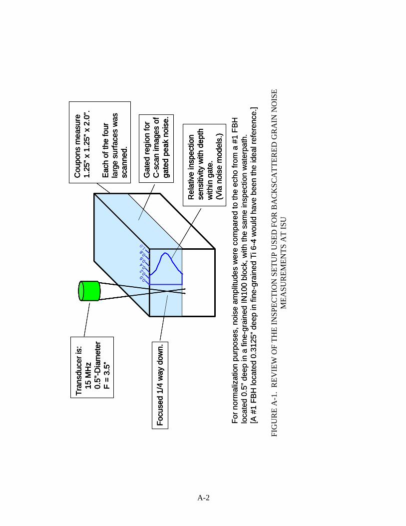
For n

orm

aliz

atio

n pu

rpos

es, n

oise

am

plitu

des

wer

e co

mpa

red

to th

e ec

ho fr

om a

#1

FBH

lo

cate

d 0.

5” d

eep

in a

fine

-gra

ined

IN10

0 bl

ock,

with

the

sam

e in

spec

tion

wat

erpa

th.

[A #

1 FB

H lo

cate

d 0.

3125

” dee

p in

fine

-gra

ined

Ti 6

-4 w

ould

hav

e be

en th

e id

eal r

efer

ence

.]

Tran

sduc

er is

:15

MH

z0.

5”-D

iam

eter

F =

3.5”

Focu

sed

1/4

way

dow

n.

Gat

ed re

gion

for

C-s

can

imag

es o

f ga

ted

peak

noi

se.

Cou

pons

mea

sure

1.25

” x 1

.25”

x 2

.0”.

Eac

h of

the

four

la

rge

surfa

ces

was

sc

anne

d.

Rel

ativ

e in

spec

tion

sens

itivi

ty w

ith d

epth

with

in g

ate.

(Via

noi

se m

odel

s.)

0.00.2

0.40.6

0.81.0

For n

orm

aliz

atio

n pu

rpos

es, n

oise

am

plitu

des

wer

e co

mpa

red

to th

e ec

ho fr

om a

#1

FBH

lo

cate

d 0.

5” d

eep

in a

fine

-gra

ined

IN10

0 bl

ock,

with

the

sam

e in

spec

tion

wat

erpa

th.

[A #

1 FB

H lo

cate

d 0.

3125

” dee

p in

fine

-gra

ined

Ti 6

-4 w

ould

hav

e be

en th

e id

eal r

efer

ence

.]

Tran

sduc

er is

:15

MH

z0.

5”-D

iam

eter

F =

3.5”

Focu

sed

1/4

way

dow

n.

Gat

ed re

gion

for

C-s

can

imag

es o

f ga

ted

peak

noi

se.

Cou

pons

mea

sure

1.25

” x 1

.25”

x 2

.0”.

Eac

h of

the

four

la

rge

surfa

ces

was

sc

anne

d.

Rel

ativ

e in

spec

tion

sens

itivi

ty w

ith d

epth

with

in g

ate.

(Via

noi

se m

odel

s.)

0.00.2

0.40.6

0.81.0

Tran

sduc

er is

:15

MH

z0.

5”-D

iam

eter

F =

3.5”

Tran

sduc

er is

:15

MH

z0.

5”-D

iam

eter

F =

3.5”

Focu

sed

1/4

way

dow

n.Fo

cuse

d 1/

4 w

ay d

own.

Gat

ed re

gion

for

C-s

can

imag

es o

f ga

ted

peak

noi

se.

Gat

ed re

gion

for

C-s

can

imag

es o

f ga

ted

peak

noi

se.

Cou

pons

mea

sure

1.25

” x 1

.25”

x 2

.0”.

Eac

h of

the

four

la

rge

surfa

ces

was

sc

anne

d.

Cou

pons

mea

sure

1.25

” x 1

.25”

x 2

.0”.

Eac

h of

the

four

la

rge

surfa

ces

was

sc

anne

d.

Rel

ativ

e in

spec

tion

sens

itivi

ty w

ith d

epth

with

in g

ate.

(Via

noi

se m

odel

s.)

Rel

ativ

e in

spec

tion

sens

itivi

ty w

ith d

epth

with

in g

ate.

(Via

noi

se m

odel

s.)

0.00.2

0.40.6

0.80.0

0.20.4

0.60.8

0.00.2

0.40.6

0.81.0

A-2

FI

GU

RE

A-1

. R

EVIE

W O

F TH

E IN

SPEC

TIO

N S

ETU

P U

SED

FO

R B

AC

KSC

ATT

ERED

GR

AIN

NO

ISE

M

EASU

REM

ENTS

AT

ISU

GE

1FW

D (

41 d

B)

OD

ID

HO

OP

0%10

0%

For t

he la

rge

rect

angu

lar c

oupo

ns th

e sc

an

area

was

1.5

” x 2

.24”

in s

teps

of 0

.02”

. A

typi

cal r

esul

t is

show

n ab

ove.

Nea

r the

bou

ndar

ies

of th

e sp

ecim

en, t

he

nois

e am

plitu

des

are

affe

cted

by

“edg

e ef

fect

s”.

“Raw

” C-s

can

for

GE

1 (B

ore

Reg

ion

Cou

pon)

Insp

ecte

d th

ru F

WD

sur

face

The

“edg

e ef

fect

ed” r

egio

ns a

re c

ropp

ed

from

the

final

imag

es. T

he d

ispl

ayed

are

a m

easu

res

abou

t 0.8

3” x

1.6

3” in

this

cas

e.

Not

e th

at in

this

exa

mpl

e, ra

dial

flow

line

s ca

n ev

iden

tly b

e se

en.

Insp

ectio

nsu

rface

and

gain

setti

ng

Labe

ls fo

r the

ad

jace

nt s

urfa

ces

whi

ch a

re p

aral

lel t

o th

e in

spec

tion

dire

ctio

n“H

oop”

(Sid

e 3)

is

alw

ays

at th

e bo

ttom

of

the

imag

e

3.5%

/ 5

.9%

Ave

rage

and

max

imum

gate

d-pe

ak n

oise

am

plitu

de,

as a

per

cent

age

of th

e am

plitu

de o

f the

#1

FBH

in

IN10

0 at

the

sam

e ga

in.

GE

1FW

D (

41 d

B)

OD

ID

HO

OP

0%10

0%0%

100%

For t

he la

rge

rect

angu

lar c

oupo

ns th

e sc

an

area

was

1.5

” x 2

.24”

in s

teps

of 0

.02”

. A

typi

cal r

esul

t is

show

n ab

ove.

Nea

r the

bou

ndar

ies

of th

e sp

ecim

en, t

he

nois

e am

plitu

des

are

affe

cted

by

“edg

e ef

fect

s”.

“Raw

” C-s

can

for

GE

1 (B

ore

Reg

ion

Cou

pon)

Insp

ecte

d th

ru F

WD

sur

face

The

“edg

e ef

fect

ed” r

egio

ns a

re c

ropp

ed

from

the

final

imag

es. T

he d

ispl

ayed

are

a m

easu

res

abou

t 0.8

3” x

1.6

3” in

this

cas

e.

Not

e th

at in

this

exa

mpl

e, ra

dial

flow

line

s ca

n ev

iden

tly b

e se

en.

Insp

ectio

nsu

rface

and

gain

setti

ng

Labe

ls fo

r the

ad

jace

nt s

urfa

ces

whi

ch a

re p

aral

lel t

o th

e in

spec

tion

dire

ctio

n“H

oop”

(Sid

e 3)

is

alw

ays

at th

e bo

ttom

of

the

imag

e

3.5%

/ 5

.9%

Ave

rage

and

max

imum

gate

d-pe

ak n

oise

am

plitu

de,

as a

per

cent

age

of th

e am

plitu

de o

f the

#1

FBH

in

IN10

0 at

the

sam

e ga

in.

A-3

FI

GU

RE

A-2

. EX

PLA

NA

TIO

N O

F C

RO

PPIN

G A

ND

LA

BEL

ING

CO

NV

ENTI

ON

S FO

R N

OIS

E

C-S

CA

NS

OF

THE

P&W

AN

D G

E FO

RG

ING

FLO

W L

INE

CO

UPO

NS

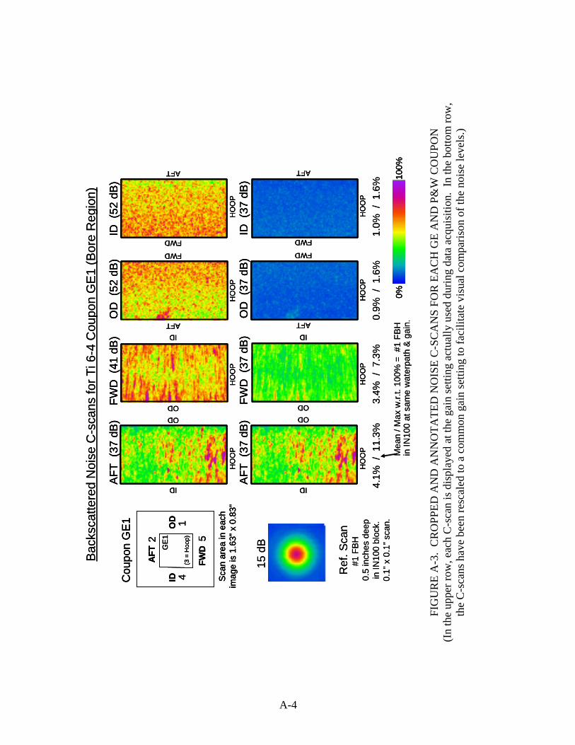
B

acks

catte

red

Noi

se C

-sca

ns fo

r Ti 6

-4 C

oupo

n G

E1

(Bor

e R

egio

n)

AFT

(37

dB

)FW

D (

41 d

B)

OD

(52

dB

)ID

(52

dB

)

ODOD

ID

ID

AFT

AFT

FWD

FWD

HO

OP

HO

OP

HO

OP

HO

OP

AFT

(37

dB

)FW

D (

37 d

B)

OD

(37

dB

)ID

(37

dB

)

ODOD

ID

ID

AFT

AFT

FWD

FWD

HO

OP

HO

OP

HO

OP

HO

OP

0%10

0%

4.1%

/ 1

1.3%

3.4%

/ 7

.3%

0.9%

/ 1

.6%

1.0%

/ 1

.6%

15 d

BGE

12

4

5

1(3

= H

oop)

AFT

FWD

IDO

D

Sca

n ar

ea in

eac

him

age

is 1

.63”

x 0

.83”

Cou

pon

GE1

Ref

. Sca

n#1

FBH

0.

5 in

ches

dee

pin

IN10

0 bl

ock.

0.1”

x 0

.1” s

can.

Mea

n / M

ax w

.r.t.

100%

= #

1 FB

Hin

IN10

0 at

sam

e w

ater

path

& g

ain.

Bac

ksca

ttere

d N

oise

C-s

cans

for T

i 6-4

Cou

pon

GE

1 (B

ore

Reg

ion)

AFT

(37

dB

)FW

D (

41 d

B)

OD

(52

dB

)ID

(52

dB

)

ODOD

ID

ID

AFT

AFT

FWD

FWD

HO

OP

HO

OP

HO

OP

HO

OP

AFT

(37

dB

)FW

D (

37 d

B)

OD

(37

dB

)ID

(37

dB

)

ODOD

ID

ID

AFT

AFT

FWD

FWD

HO

OP

HO

OP

HO

OP

HO

OP

AFT

(37

dB

)FW

D (

41 d

B)

OD

(52

dB

)ID

(52

dB

)

ODOD

ID

ID

AFT

AFT

FWD

FWD

HO

OP

HO

OP

HO

OP

HO

OP

AFT

(37

dB

)FW

D (

37 d

B)

OD

(37

dB

)ID

(37

dB

)

ODOD

ID

ID

AFT

AFT

FWD

FWD

HO

OP

HO

OP

HO

OP

HO

OP

0%10

0%0%

100%

4.1%

/ 1

1.3%

3.4%

/ 7

.3%

0.9%

/ 1

.6%

1.0%

/ 1

.6%

15 d

BGE

12

4

5

1(3

= H

oop)

AFT

FWD

IDO

D

Sca

n ar

ea in

eac

him

age

is 1

.63”

x 0

.83”

Cou

pon

GE1

GE

12

4

5

1(3

= H

oop)

AFT

FWD

IDO

D

Sca

n ar

ea in

eac

him

age

is 1

.63”

x 0

.83”

Cou

pon

GE1

Ref

. Sca

n#1

FBH

0.

5 in

ches

dee

pin

IN10

0 bl

ock.

0.1”

x 0

.1” s

can.

Mea

n / M

ax w

.r.t.

100%

= #

1 FB

Hin

IN10

0 at

sam

e w

ater

path

& g

ain.

A-4

FI

GU

RE

A-3

. C

RO

PPED

AN

D A

NN

OTA

TED

NO

ISE

C-S

CA

NS

FOR

EA

CH

GE

AN

D P

&W

CO

UPO

N

(In

the

uppe

r row

, eac

h C

-sca

n is

dis

play

ed a

t the

gai

n se

tting

act

ually

use

d du

ring

data

acq

uisi

tion.

In

the

botto

m ro

w,

the

C-s

cans

hav

e be

en re

scal

ed to

a c

omm

on g

ain

setti

ng to

faci

litat

e vi

sual

com

paris

on o

f the

noi

se le

vels

.)

B

acks

catte

red

Noi

se C

-sca

ns fo

r Ti 6

-4 C

oupo

n G

E4

(Far

Rim

Reg

ion;

Mid

Thi

ckne

ss)

0%10

0%

1.7%

/ 5

.5%

1.4%

/ 3

.5%

5.6%

/ 1

5.0%

3.6%

/ 8

.8%

AFT

(45

dB)

FWD

(45

dB

)O

D (

34 d

B)ID

(36

dB)

ODOD

ID

ID

AFT

AFT

FWDFWD

HO

OP

HO

OP

HO

OP

HO

OP

AFT

(34

dB)

FWD

(34

dB)

OD

(34

dB)

ID (

34 d

B)

ODOD

ID

ID

AFT

AFT

FWDFWD

HO

OP

HO

OP

HO

OP

HO

OP

15 d

BGE

42

4

5

1(3

= H

oop)

AFT

FWD

IDO

D

Sca

n ar

ea in

eac

him

age

is 1

.63”

x 0

.83”

Cou

pon

GE

4

Ref

. Sca

n#1

FB

H

0.5

inch

es d

eep

in IN

100

bloc

k.0.

1” x

0.1

” sca

n.M

ean

/ Max

w.r.

t. 10

0% =

#1

FBH

in IN

100

at s

ame

wat

erpa

th &

gai

n.

Bac

ksca

ttere

d N

oise

C-s

cans

for T

i 6-4

Cou

pon

GE

4 (F

ar R

im R

egio

n; M

id T

hick

ness

)

0%10

0%0%

100%

1.7%

/ 5

.5%

1.4%

/ 3

.5%

5.6%

/ 1

5.0%

3.6%

/ 8

.8%

AFT

(45

dB)

FWD

(45

dB

)O

D (

34 d

B)ID

(36

dB)

ODOD

ID

ID

AFT

AFT

FWDFWD

HO

OP

HO

OP

HO

OP

HO

OP

AFT

(34

dB)

FWD

(34

dB)

OD

(34

dB)

ID (

34 d

B)

ODOD

ID

ID

AFT

AFT

FWDFWD

HO

OP

HO

OP

HO

OP

HO

OP

AFT

(45

dB)

FWD

(45

dB

)O

D (

34 d

B)ID

(36

dB)

ODOD

ID

ID

AFT

AFT

FWDFWD

HO

OP

HO

OP

HO

OP

HO

OP

AFT

(34

dB)

FWD

(34

dB)

OD

(34

dB)

ID (

34 d

B)

ODOD

ID

ID

AFT

AFT

FWDFWD

HO

OP

HO

OP

HO

OP

HO

OP

15 d

BGE

42

4

5

1(3

= H

oop)

AFT

FWD

IDO

D

Sca

n ar

ea in

eac

him

age

is 1

.63”

x 0

.83”

Cou

pon

GE

4

GE

42

4

5

1(3

= H

oop)

AFT

FWD

IDO

D

Sca

n ar

ea in

eac

him

age

is 1

.63”

x 0

.83”

Cou

pon

GE

4

Ref

. Sca

n#1

FB

H

0.5

inch

es d

eep

in IN

100

bloc

k.0.

1” x

0.1

” sca

n.M

ean

/ Max

w.r.

t. 10

0% =

#1

FBH

in IN

100

at s

ame

wat

erpa

th &

gai

n.

A-5

FI

GU

RE

A-3

. C

RO

PPED

AN

D A

NN

OTA

TED

NO

ISE

C-S

CA

NS

FOR

EA

CH

GE

AN

D P

&W

CO

UPO

N (C

ontin

ued)

(I

n th

e up

per r

ow, e

ach

C-s

can

is d

ispl

ayed

at t

he g

ain

setti

ng a

ctua

lly u

sed

durin

g da

ta a

cqui

sitio

n. I

n th

e bo

ttom

row

, th

e C

-sca

ns h

ave

been

resc

aled

to a

com

mon

gai

n se

tting

to fa

cilit

ate

visu

al c

ompa

rison

of t

he n

oise

leve

ls.)

B

acks

catte

red

Noi

se C

-sca

ns fo

r Ti 6

-4 C

oupo

n G

E5

(Far

Rim

Reg

ion,

FW

D S

ide)

0%10

0%

1.3%

/ 3

.2%

1.0%

/ 1

.7%

3.3%

/ 1

2.0%

3.1%

/ 1

1.4%

AFT

(45

dB

)FW

D (

48 d

B)

OD

(36

dB

)ID

(36

dB

)

ODOD

ID

ID

AFT

AFT

FWD

FWD

HO

OP

HO

OP

HO

OP

HO

OP

AFT

(36

dB

)FW

D (

36 d

B)

OD

(36

dB

)ID

(36

dB

)

ODOD

ID

ID

AFT

AFT

FWDFWD

HO

OP

HO

OP

HO

OP

HO

OP

15 d

BGE

52

4

5

1(3

= H

oop)

AFT

FWD

IDO

D

Scan

are

a in

eac

him

age

is 1

.63”

x 0

.83”

Cou

pon

GE

5

Ref

. Sca

n#1

FB

H

0.5

inch

es d

eep

in IN

100

bloc

k.0.

1” x

0.1

” sca

n.M

ean

/ Max

w.r.

t. 10

0% =

#1

FBH

in IN

100

at s

ame

wat

erpa

th &

gai

n.

Bac

ksca

ttere

d N

oise

C-s

cans

for T

i 6-4

Cou

pon

GE

5 (F

ar R

im R

egio

n, F

WD

Sid

e)

0%10

0%0%

100%

1.3%

/ 3

.2%

1.0%

/ 1

.7%

3.3%

/ 1

2.0%

3.1%

/ 1

1.4%

AFT

(45

dB

)FW

D (

48 d

B)

OD

(36

dB

)ID

(36

dB

)

ODOD

ID

ID

AFT

AFT

FWD

FWD

HO

OP

HO

OP

HO

OP

HO

OP

AFT

(36

dB

)FW

D (

36 d

B)

OD

(36

dB

)ID

(36

dB

)

ODOD

ID

ID

AFT

AFT

FWDFWD

HO

OP

HO

OP

HO

OP

HO

OP

AFT

(45

dB

)FW

D (

48 d

B)

OD

(36

dB

)ID

(36

dB

)

ODOD

ID

ID

AFT

AFT

FWD

FWD

HO

OP

HO

OP

HO

OP

HO

OP

AFT

(36

dB

)FW

D (

36 d

B)

OD

(36

dB

)ID

(36

dB

)

ODOD

ID

ID

AFT

AFT

FWDFWD

HO

OP

HO

OP

HO

OP

HO

OP

15 d

BGE

52

4

5

1(3

= H

oop)

AFT

FWD

IDO

D

Scan

are

a in

eac

him

age

is 1

.63”

x 0

.83”

Cou

pon

GE

5

GE

52

4

5

1(3

= H

oop)

AFT

FWD

IDO

D

Scan

are

a in

eac

him

age

is 1

.63”

x 0

.83”

Cou

pon

GE

5

Ref

. Sca

n#1

FB

H

0.5

inch

es d

eep

in IN

100

bloc

k.0.

1” x

0.1

” sca

n.M

ean

/ Max

w.r.

t. 10

0% =

#1

FBH

in IN

100

at s

ame

wat

erpa

th &

gai

n.

A-6

FI

GU

RE

A-3

. C

RO

PPED

AN

D A

NN

OTA

TED

NO

ISE

C-S

CA

NS

FOR

EA

CH

GE

AN

D P

&W

CO

UPO

N (C

ontin

ued)

(I

n th

e up

per r

ow, e

ach

C-s

can

is d

ispl

ayed

at t

he g

ain

setti

ng a

ctua

lly u

sed

durin

g da

ta a

cqui

sitio

n. I

n th

e bo

ttom

row

, th

e C

-sca

ns h

ave

been

resc

aled

to a

com

mon

gai

n se

tting

to fa

cilit

ate

visu

al c

ompa

rison

of t

he n

oise

leve

ls.)

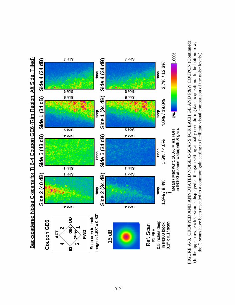
Bac

ksca

ttere

d N

oise

C-s

cans

for T

i 6-4

Cou

pon

GE

6 (R

im R

egio

n, A

ft S

ide,

Tilt

ed)

0%10

0%

1.9%

/ 8.

4%1.

5% /

4.0%

4.0%

/ 19

.0%

2.7%

/ 12

.3%

Side

2 (4

0 dB

)Si

de 5

(43

dB)

Side

1 (3

4 dB

)Si

de 4

(34

dB)

Side 1

Side 4H

oop

Side 1

Side 4

Hoo

pH

oop

Hoo

p

Side 2

Side 5

Side 5

Side 2

Side

2 (3

4 dB

)Si

de 5

(34

dB)

Sid

e 1

(34

dB)

Side

4 (3

4 dB

)

Side 1

Side 4

Hoo

p

Side 1

Side 4

Hoo

pH

oop

Hoo

p

Side 2

Side 5

Side 5

Side 2

15 d

BGE

624 5

1(H

oop)

AFT

FWD

IDO

D

Scan

are

a in

eac

him

age

is 1

.63”

x 0

.83”

Cou

pon

GE6

Ref

. Sca

n#1

FB

H

0.5

inch

es d

eep

in IN

100

bloc

k.0.

1” x

0.1

” sca

n.M

ean

/ Max

w.r.

t. 10

0% =

#1

FBH

in IN

100

at s

ame

wat

erpa

th &

gai

n.

Bac

ksca

ttere

d N

oise

C-s

cans

for T

i 6-4

Cou

pon

GE

6 (R

im R

egio

n, A

ft S

ide,

Tilt

ed)

0%10

0%0%

100%

1.9%

/ 8.

4%1.

5% /

4.0%

4.0%

/ 19

.0%

2.7%

/ 12

.3%

Side

2 (4

0 dB

)Si

de 5

(43

dB)

Side

1 (3

4 dB

)Si

de 4

(34

dB)

Side 1

Side 4H

oop

Side 1

Side 4

Hoo

pH

oop

Hoo

p

Side 2

Side 5

Side 5

Side 2

Side

2 (3

4 dB

)Si

de 5

(34

dB)

Sid

e 1

(34

dB)

Side

4 (3

4 dB

)

Side 1

Side 4

Hoo

p

Side 1

Side 4

Hoo

pH

oop

Hoo

p

Side 2

Side 5

Side 5

Side 2

Side

2 (4

0 dB

)Si

de 5

(43

dB)

Side

1 (3

4 dB

)Si

de 4

(34

dB)

Side 1

Side 4H

oop

Side 1

Side 4

Hoo

pH

oop

Hoo

p

Side 2

Side 5

Side 5

Side 2

Side

2 (3

4 dB

)Si

de 5

(34

dB)

Sid

e 1

(34

dB)

Side

4 (3

4 dB

)

Side 1

Side 4

Hoo

p

Side 1

Side 4

Hoo

pH

oop

Hoo

p

Side 2

Side 5

Side 5

Side 2

15 d

BGE

624 5

1(H

oop)

AFT

FWD

IDO

D

Scan

are

a in

eac

him

age

is 1

.63”

x 0

.83”

Cou

pon

GE6

GE

624 5

1(H

oop)

AFT

FWD

IDO

DG

E62

4 51

(Hoo

p)

AFT

FWD

IDO

D

Scan

are

a in

eac

him

age

is 1

.63”

x 0

.83”

Cou

pon

GE6

Ref

. Sca

n#1

FB

H

0.5

inch

es d

eep

in IN

100

bloc

k.0.

1” x

0.1

” sca

n.M

ean

/ Max

w.r.

t. 10

0% =

#1

FBH

in IN

100

at s

ame

wat

erpa

th &

gai

n.

A-7

FI

GU

RE

A-3

. C

RO

PPED

AN

D A

NN

OTA

TED

NO

ISE

C-S

CA

NS

FOR

EA

CH

GE

AN

D P

&W

CO

UPO

N (C

ontin

ued)

(I

n th

e up

per r

ow, e

ach

C-s

can

is d

ispl

ayed

at t

he g

ain

setti

ng a

ctua

lly u

sed

durin

g da

ta a

cqui

sitio

n. I

n th

e bo

ttom

row

, th

e C

-sca

ns h

ave

been

resc

aled

to a

com

mon

gai

n se

tting

to fa

cilit

ate

visu

al c

ompa

rison

of t

he n

oise

leve

ls.)

Back

scat

tere

d N

oise

C-s

cans

for T

i 6-4

Cou

pon

GE7

(Rim

Reg

ion,

FW

D S

ide,

Tilt

ed)

0%10

0%

3.2%

/ 8.

3%3.

8% /

10.4

%1.

5% /

3.0%

1.4%

/ 2.

8%

Side

2 (3

7 dB

)S

ide

5 (3

5 dB

)S

ide

1 (4

5 dB

)S

ide

4 (4

5 dB

)

Side 1

Side 4H

oop

Side 1

Side 4

Hoo

pH

oop

Hoo

p

Side 2

Side 5

Side 5

Side 2

Side

2 (3

5 dB

)S

ide

5 (3

5 dB

)S

ide

1 (3

5 dB

)S

ide

4 (3

5 dB

)

Side 1

Side 4

Hoo

p

Side 1

Side 4

Hoo

pH

oop

Hoo

p

Side 2

Side 5

Side 5

Side 2

Mea

n / M

ax w

.r.t.

100%

= #

1 FB

Hin

IN10

0 at

sam

e w

ater

path

& g

ain.

15 d

BGE

724 5

1(H

oop)

AFT

FWD

IDO

D

Scan

are

a in

eac

him

age

is 1

.63”

x 0

.83”

Cou

pon

GE7

Ref

. Sca

n#1

FBH

0.

5 in

ches

dee

pin

IN10

0 bl

ock.

0.1”

x 0

.1” s

can.

Back

scat

tere

d N

oise

C-s

cans

for T

i 6-4

Cou

pon

GE7

(Rim

Reg

ion,

FW

D S

ide,

Tilt

ed)

0%10

0%0%

100%

3.2%

/ 8.

3%3.

8% /

10.4

%1.

5% /

3.0%

1.4%

/ 2.

8%

Side

2 (3

7 dB

)S

ide

5 (3

5 dB

)S

ide

1 (4

5 dB

)S

ide

4 (4

5 dB

)

Side 1

Side 4H

oop

Side 1

Side 4

Hoo

pH

oop

Hoo

p

Side 2

Side 5

Side 5

Side 2

Side

2 (3

5 dB

)S

ide

5 (3

5 dB

)S

ide

1 (3

5 dB

)S

ide

4 (3

5 dB

)

Side 1

Side 4

Hoo

p

Side 1

Side 4

Hoo

pH

oop

Hoo

p

Side 2

Side 5

Side 5

Side 2

3.2%

/ 8.

3%3.

8% /

10.4

%1.

5% /

3.0%

1.4%

/ 2.

8%

Side

2 (3

7 dB

)S

ide

5 (3

5 dB

)S

ide

1 (4

5 dB

)S

ide

4 (4

5 dB

)

Side 1

Side 4H

oop

Side 1

Side 4

Hoo

pH

oop

Hoo

p

Side 2

Side 5

Side 5

Side 2

Side

2 (3

5 dB

)S

ide

5 (3

5 dB

)S

ide

1 (3

5 dB

)S

ide

4 (3

5 dB

)

Side 1

Side 4

Hoo

p

Side 1

Side 4

Hoo

pH

oop

Hoo

p

Side 2

Side 5

Side 5

Side 2

Mea

n / M

ax w

.r.t.

100%

= #

1 FB

Hin

IN10

0 at

sam

e w

ater

path

& g

ain.

15 d

BGE

724 5

1(H

oop)

AFT

FWD

IDO

D

Scan

are

a in

eac

him

age

is 1

.63”

x 0

.83”

Cou

pon

GE7

GE

724 5

1(H

oop)

AFT

FWD

IDO

DG

E72

4 51

(Hoo

p)

AFT

FWD

IDO

D

Scan

are

a in

eac

him

age

is 1

.63”

x 0

.83”

Cou

pon

GE7

Ref

. Sca

n#1

FBH

0.

5 in

ches

dee

pin

IN10

0 bl

ock.

0.1”

x 0

.1” s

can.

A-8

FI

GU

RE

A-3

. C

RO

PPED

AN

D A

NN

OTA

TED

NO

ISE

C-S

CA

NS

FOR

EA

CH

GE

AN

D P

&W

CO

UPO

N (C

ontin

ued)

(I

n th

e up

per r

ow, e

ach

C-s

can

is d

ispl

ayed

at t

he g

ain

setti

ng a

ctua

lly u

sed

durin

g da

ta a

cqui

sitio

n. I

n th

e bo

ttom

row

, th

e C

-sca

ns h

ave

been

resc

aled

to a

com

mon

gai

n se

tting

to fa

cilit

ate

visu

al c

ompa

rison

of t

he n

oise

leve

ls.)

Bac

ksca

ttere

d N

oise

C-s

cans

for T

i 6-4

Cou

pon

PW

1 (B

ore

Reg

ion)

TOP

(42

dB)

BO

T (3

7 dB

)O

D (

42 d

B)ID

(42

dB)

ODOD

ID

ID

TOP

TOP

BOT

BOT

HO

OP

HO

OP

HO

OP

HO

OP

TOP

(37

dB)

BOT

(37

dB)

OD

(37

dB)

ID (

37 d

B)

ODOD

ID

ID

TOP

TOP

BOT

BOT

HO

OP

HO

OP

HO

OP

HO

OP

0%10

0%

2.4%

/ 6

.3%

3.8%

/ 1

0.7%

1.8%

/ 6

.3%

1.9%

/ 6

.7%

17 d

B

Ref

. Sca

n#1

FB

H

0.5

inch

es d

eep

in IN

100

bloc

k.0.

1” x

0.1

” sca

n.M

ean

/ Max

w.r.

t. 10

0% =

#1

FBH

in IN

100

at s

ame

wat

erpa

th &

gai

n.

#12

4

5

1

(3 =

Hoo

p)

TOP

BO

T

IDO

D

Dis

play

ed a

rea

in e

ach

imag

e is

1.6

3” x

0.8

3”

Cou

pon

PW1

Bac

ksca

ttere

d N

oise

C-s

cans

for T

i 6-4

Cou

pon

PW

1 (B

ore

Reg

ion)

TOP

(42

dB)

BO

T (3

7 dB

)O

D (

42 d

B)ID

(42

dB)

ODOD

ID

ID

TOP

TOP

BOT

BOT

HO

OP

HO

OP

HO

OP

HO

OP

TOP

(37

dB)

BOT

(37

dB)

OD

(37

dB)

ID (

37 d

B)

ODOD

ID

ID

TOP

TOP

BOT

BOT

HO

OP

HO

OP

HO

OP

HO

OP

0%10

0%0%

100%

2.4%

/ 6

.3%

3.8%

/ 1

0.7%

1.8%

/ 6

.3%

1.9%

/ 6

.7%

17 d

B

Ref

. Sca

n#1

FB

H

0.5

inch

es d

eep

in IN

100

bloc

k.0.

1” x

0.1

” sca

n.M

ean

/ Max

w.r.

t. 10

0% =

#1

FBH

in IN

100

at s

ame

wat

erpa

th &

gai

n.

#12

4

5

1

(3 =

Hoo

p)

TOP

BO

T

IDO

D

Dis

play

ed a

rea

in e

ach

imag

e is

1.6

3” x

0.8

3”

Cou

pon

PW1

#12

4

5

1

(3 =

Hoo

p)

TOP

BO

T

IDO

D

Dis

play

ed a

rea

in e

ach

imag

e is

1.6

3” x

0.8

3”

Cou

pon

PW1

A-9

FI

GU

RE

A-3

. C

RO

PPED

AN

D A

NN

OTA

TED

NO

ISE

C-S

CA

NS

FOR

EA

CH

GE

AN

D P

&W

CO

UPO

N (C

ontin

ued)

(I

n th

e up

per r

ow, e

ach

C-s

can

is d

ispl

ayed

at t

he g

ain

setti

ng a

ctua

lly u

sed

durin

g da

ta a

cqui

sitio

n. I

n th

e bo

ttom

row

, th

e C

-sca

ns h

ave

been

resc

aled

to a

com

mon

gai

n se

tting

to fa

cilit

ate

visu

al c

ompa

rison

of t

he n

oise

leve

ls.)

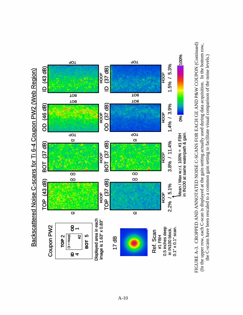
Bac

ksca

ttere

d N

oise

C-s

cans

for T

i 6-4

Cou

pon

PW

2 (W

eb R

egio

n)

TOP

(43

dB)

BO

T (3

7 dB

)O

D (

46 d

B)ID

(43

dB)

ODOD

ID

ID

TOP

TOP

BOT

BOT

HO

OP

HO

OP

HO

OP

HO

OP

TOP

(37

dB)

BOT

(37

dB)

OD

(37

dB)

ID (

37 d

B)

ODOD

ID

ID

TOP

TOP

BOT

BOT

HO

OP

HO

OP

HO

OP

HO

OP

0%10

0%

2.2%

/ 5

.1%

3.8%

/ 1

1.4%

1.4%

/ 3

.9%

1.5%

/ 5

.3%

17 d

B

Ref

. Sca

n#1

FB

H

0.5

inch

es d

eep

in IN

100

bloc

k.0.

1” x

0.1

” sca

n.M

ean

/ Max

w.r.

t. 10

0% =

#1

FBH

in IN

100

at s

ame

wat

erpa

th &

gai

n.

#22

4

5

1

(3 =

Hoo

p)

TOP

BO

T

IDO

D

Dis

play

ed a

rea

in e

ach

imag

e is

1.6

3” x

0.8

3”

Cou

pon

PW2

Bac

ksca

ttere

d N

oise

C-s

cans

for T

i 6-4

Cou

pon

PW

2 (W

eb R

egio

n)

TOP

(43

dB)

BO

T (3

7 dB

)O

D (

46 d

B)ID

(43

dB)

ODOD

ID

ID

TOP

TOP

BOT

BOT

HO

OP

HO

OP

HO

OP

HO

OP

TOP

(37

dB)

BOT

(37

dB)

OD

(37

dB)

ID (

37 d

B)

ODOD

ID

ID

TOP

TOP

BOT

BOT

HO

OP

HO

OP

HO

OP

HO

OP

TOP

(43

dB)

BO

T (3

7 dB

)O

D (

46 d

B)ID

(43

dB)

ODOD

ID

ID

TOP

TOP

BOT

BOT

HO

OP

HO

OP

HO

OP

HO

OP

TOP

(37

dB)

BOT

(37

dB)

OD

(37

dB)

ID (

37 d

B)

ODOD

ID

ID

TOP

TOP

BOT

BOT

HO

OP

HO

OP

HO

OP

HO

OP

0%10

0%0%

100%

2.2%

/ 5

.1%

3.8%

/ 1

1.4%

1.4%

/ 3

.9%

1.5%

/ 5

.3%

17 d

B

Ref

. Sca

n#1

FB

H

0.5

inch

es d

eep

in IN

100

bloc

k.0.

1” x

0.1

” sca

n.M

ean

/ Max

w.r.

t. 10

0% =

#1

FBH

in IN

100

at s

ame

wat

erpa

th &

gai

n.

#22

4

5

1

(3 =

Hoo

p)

TOP

BO

T

IDO

D

Dis

play

ed a

rea

in e

ach

imag

e is

1.6

3” x

0.8

3”

Cou

pon

PW2

#22

4

5

1

(3 =

Hoo

p)

TOP

BO

T

IDO

D

Dis

play

ed a

rea

in e

ach

imag

e is

1.6

3” x

0.8

3”

Cou

pon

PW2

A-10

FI

GU

RE

A-3

. C

RO

PPED

AN

D A

NN

OTA

TED

NO

ISE

C-S

CA

NS

FOR

EA

CH

GE

AN

D P

&W

CO

UPO

N (C

ontin

ued)

(I

n th

e up

per r

ow, e

ach

C-s

can

is d

ispl

ayed

at t

he g

ain

setti

ng a

ctua

lly u

sed

durin

g da

ta a

cqui

sitio

n. I

n th

e bo

ttom

row

, th

e C

-sca

ns h

ave

been

resc

aled

to a

com

mon

gai

n se

tting

to fa

cilit

ate

visu

al c

ompa

rison

of t

he n

oise

leve

ls.)

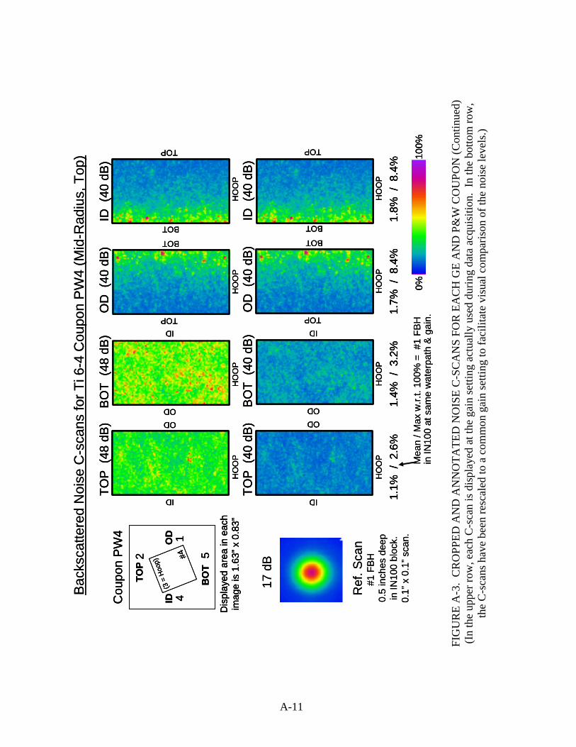
Bac

ksca

ttere

d N

oise

C-s

cans

for T

i 6-4

Cou

pon

PW

4 (M

id-R

adiu

s, T

op)

0%10

0%

TOP

(48

dB

)B

OT

(48

dB)

OD

(40

dB

)ID

(40

dB

)

ODOD

ID

ID

TOP

TOP

BOT

BOT

HO

OP

HO

OP

HO

OP

HO

OP

TOP

(40

dB

)B

OT

(40

dB)

OD

(40

dB

)ID

(40

dB

)

ODOD

ID

ID

TOP

TOP

BOT

BOT

HO

OP

HO

OP

HO

OP

HO

OP

1.1%

/ 2

.6%

1.4%

/ 3

.2%

1.7%

/ 8

.4%

1.8%

/ 8

.4%

17 d

B#42

4

5

1(3

= H

oop)

TOP

BO

T

IDO

D

Dis

play

ed a

rea

in e

ach

imag

e is

1.6

3” x

0.8

3”

Cou

pon

PW

4

Ref

. Sca

n#1

FB

H

0.5

inch

es d

eep

in IN

100

bloc

k.0.

1” x

0.1

” sca

n.M

ean

/ Max

w.r.

t. 10

0% =

#1

FBH

in IN

100

at s

ame

wat

erpa

th &

gai

n.

Bac

ksca

ttere

d N

oise

C-s

cans

for T

i 6-4

Cou

pon

PW

4 (M

id-R

adiu

s, T

op)

0%10

0%0%

100%

TOP

(48

dB

)B

OT

(48

dB)

OD

(40

dB

)ID

(40

dB

)

ODOD

ID

ID

TOP

TOP

BOT

BOT

HO

OP

HO

OP

HO

OP

HO

OP

TOP

(40

dB

)B

OT

(40

dB)

OD

(40

dB

)ID

(40

dB

)

ODOD

ID

ID

TOP

TOP

BOT

BOT

HO

OP

HO

OP

HO

OP

HO

OP

1.1%

/ 2

.6%

1.4%

/ 3

.2%

1.7%

/ 8

.4%

1.8%

/ 8

.4%

TOP

(48

dB

)B

OT

(48

dB)

OD

(40

dB

)ID

(40

dB

)

ODOD

ID

ID

TOP

TOP

BOT

BOT

HO

OP

HO

OP

HO

OP

HO

OP

TOP

(40

dB

)B

OT

(40

dB)

OD

(40

dB

)ID

(40

dB

)

ODOD

ID

ID

TOP

TOP

BOT

BOT

HO

OP

HO

OP

HO

OP

HO

OP

1.1%

/ 2

.6%

1.4%

/ 3

.2%

1.7%

/ 8

.4%

1.8%

/ 8

.4%

17 d

B#42

4

5

1(3

= H

oop)

TOP

BO

T

IDO

D

Dis

play

ed a

rea

in e

ach

imag

e is

1.6

3” x

0.8

3”

Cou

pon

PW

4

#42

4

5

1(3

= H

oop)

TOP

BO

T

IDO

D

Dis

play

ed a

rea

in e

ach

imag

e is

1.6

3” x

0.8

3”

Cou

pon

PW

4

Ref

. Sca

n#1

FB

H

0.5

inch

es d

eep

in IN

100

bloc

k.0.

1” x

0.1

” sca

n.M

ean

/ Max

w.r.

t. 10

0% =

#1

FBH

in IN

100

at s

ame

wat

erpa

th &

gai

n.

A-11

FI

GU

RE

A-3

. C

RO

PPED

AN

D A

NN

OTA

TED

NO

ISE

C-S

CA

NS

FOR

EA

CH

GE

AN

D P

&W

CO

UPO

N (C

ontin

ued)

(I

n th

e up

per r

ow, e

ach

C-s

can

is d

ispl

ayed

at t

he g

ain

setti

ng a

ctua

lly u

sed

durin

g da

ta a

cqui

sitio

n. I

n th

e bo

ttom

row

, th

e C

-sca

ns h

ave

been

resc

aled

to a

com

mon

gai

n se

tting

to fa

cilit

ate

visu

al c

ompa

rison

of t

he n

oise

leve

ls.)

Back

scat

tere

d N

oise

C-s

cans

for T

i 6-4

Cou

pon

PW5

(Mid

-Rad

ius;

Cen

ter)

TOP

(41

dB)

BOT

(41

dB)

OD

(35

dB)

ID (

35 d

B)

ODOD

ID

ID

TOP

TOP

BOT

BOT

HO

OP

HO

OP

HO

OP

HO

OP

TOP

(35

dB)

BO

T (3

5 dB

)O

D (

35 d

B)ID

(35

dB)

ODOD

ID

ID

TOP

TOP

BOT

BOT

HO

OP

HO

OP

HO

OP

HO

OP

0%10

0%

2.5%

/ 6

.9%

2.2%

/ 7

.3%

3.5%

/ 1

2.4%

3.0%

/ 1

3.9%

17 d

B#52

4

5

1

(3 =

Hoo

p)

TOP

BO

T

IDO

D

Dis

play

ed a

rea

in e

ach

imag

e is

1.6

3” x

0.8

3”

Cou

pon

PW5

Ref

. Sca

n#1

FB

H

0.5

inch

es d

eep

in IN

100

bloc

k.0.

1” x

0.1

” sca

n.M

ean

/ Max

w.r.

t. 10

0% =

#1

FBH

in IN

100

at s

ame

wat

erpa

th &

gai

n.

Back

scat

tere

d N

oise

C-s

cans

for T

i 6-4

Cou

pon

PW5

(Mid

-Rad

ius;

Cen

ter)

TOP

(41

dB)

BOT

(41

dB)

OD

(35

dB)

ID (

35 d

B)

ODOD

ID

ID

TOP

TOP

BOT

BOT

HO

OP

HO

OP

HO

OP

HO

OP

TOP

(35

dB)

BO

T (3

5 dB

)O

D (

35 d

B)ID

(35

dB)

ODOD

ID

ID

TOP

TOP

BOT

BOT

HO

OP

HO

OP

HO

OP

HO

OP

TOP

(41

dB)

BOT

(41

dB)

OD

(35

dB)

ID (

35 d

B)

ODOD

ID

ID

TOP

TOP

BOT

BOT

HO

OP

HO

OP

HO

OP

HO

OP

TOP

(35

dB)

BO

T (3

5 dB

)O

D (

35 d

B)ID

(35

dB)

ODOD

ID

ID

TOP

TOP

BOT

BOT

HO

OP

HO

OP

HO

OP

HO

OP

0%10

0%0%

100%

2.5%

/ 6

.9%

2.2%

/ 7

.3%

3.5%

/ 1

2.4%

3.0%

/ 1

3.9%

17 d

B#52

4

5

1

(3 =

Hoo

p)

TOP

BO

T

IDO

D

Dis

play

ed a

rea

in e

ach

imag

e is

1.6

3” x

0.8

3”

Cou

pon

PW5

#52

4

5

1

(3 =

Hoo

p)

TOP

BO

T

IDO

D

Dis

play

ed a

rea

in e

ach

imag

e is

1.6

3” x

0.8

3”

Cou

pon

PW5

Ref

. Sca

n#1

FB

H

0.5

inch

es d

eep

in IN

100

bloc

k.0.

1” x

0.1

” sca

n.M

ean

/ Max

w.r.

t. 10

0% =

#1

FBH

in IN

100

at s

ame

wat

erpa

th &

gai

n.

A-12

FI

GU

RE

A-3

. C

RO

PPED

AN

D A

NN

OTA

TED

NO

ISE

C-S

CA

NS

FOR

EA

CH

GE

AN

D P

&W

CO

UPO

N (C

ontin

ued)

(I

n th

e up

per r

ow, e

ach

C-s

can

is d

ispl

ayed

at t

he g

ain

setti

ng a

ctua

lly u

sed

durin

g da

ta a

cqui

sitio

n. I

n th

e bo

ttom

row

, th

e C

-sca

ns h

ave

been

resc

aled

to a

com

mon

gai

n se

tting

to fa

cilit

ate

visu

al c

ompa

rison

of t

he n

oise

leve

ls.)

Bac

ksca

ttere

d N

oise

C-s

cans

for T

i 6-4

Cou

pon

PW

6 (M

id-R

adiu

s, B

otto

m)

TOP

(41

dB)

BO

T (4

1 dB

)O

D (

35 d

B)ID

(35

dB

)

ODOD

ID

ID

TOP

TOP

BOT

BOT

HO

OP

HO

OP

HO

OP

HO

OP

TOP

(35

dB)

BO

T (3

5 dB

)O

D (

35 d

B)ID

(35

dB)

ODOD

ID

ID

TOP

TOP

BOT

BOT

HO

OP

HO

OP

HO

OP

HO

OP

0%10

0%

2.1%

/ 6

.1%

1.8%

/ 5

.4%

3.9%

/ 1

3.3%

3.4%

/ 1

4.5%

17 d

B#62

4

5

1

(3 =

Hoo

p)

TOP

BO

T

IDO

D

Dis

play

ed a

rea

in e

ach

imag

e is

1.6

3” x

0.8

3”

Cou

pon

PW6

Ref

. Sca

n#1

FBH

0.

5 in

ches

dee

pin

IN10

0 bl

ock.

0.1”

x 0

.1” s

can.

Mea

n / M

ax w

.r.t.

100%

= #

1 FB

Hin

IN10

0 at

sam

e w

ater

path

& g

ain.

Bac

ksca

ttere

d N

oise

C-s

cans

for T

i 6-4

Cou

pon

PW

6 (M

id-R

adiu

s, B

otto

m)

TOP

(41

dB)

BO

T (4

1 dB

)O

D (

35 d

B)ID

(35

dB

)

ODOD

ID

ID

TOP

TOP

BOT

BOT

HO

OP

HO

OP

HO

OP

HO

OP

TOP

(35

dB)

BO

T (3

5 dB

)O

D (

35 d

B)ID

(35

dB)

ODOD

ID

ID

TOP

TOP

BOT

BOT

HO

OP

HO

OP

HO

OP

HO

OP

TOP

(41

dB)

BO

T (4

1 dB

)O

D (

35 d

B)ID

(35

dB

)

ODOD

ID

ID

TOP

TOP

BOT

BOT

HO

OP

HO

OP

HO

OP

HO

OP

TOP

(35

dB)

BO

T (3

5 dB

)O

D (

35 d

B)ID

(35

dB)

ODOD

ID

ID

TOP

TOP

BOT

BOT

HO

OP

HO

OP

HO

OP

HO

OP

0%10

0%0%

100%

2.1%

/ 6

.1%

1.8%

/ 5

.4%

3.9%

/ 1

3.3%

3.4%

/ 1

4.5%

17 d

B#62

4

5

1

(3 =

Hoo

p)

TOP

BO

T

IDO

D

Dis

play

ed a

rea

in e

ach

imag

e is

1.6

3” x

0.8

3”

Cou

pon

PW6

#62

4

5

1

(3 =

Hoo

p)

TOP

BO

T

IDO

D

Dis

play

ed a

rea

in e

ach

imag

e is

1.6

3” x

0.8

3”

Cou

pon

PW6

Ref

. Sca

n#1

FBH

0.

5 in

ches

dee

pin

IN10

0 bl

ock.

0.1”

x 0

.1” s

can.

Mea

n / M

ax w

.r.t.

100%

= #

1 FB

Hin

IN10

0 at

sam

e w

ater

path

& g

ain.

A-13

FI

GU

RE

A-3

. C

RO

PPED

AN

D A

NN

OTA

TED

NO

ISE

C-S

CA

NS

FOR

EA

CH

GE

AN

D P

&W

CO

UPO

N (C

ontin

ued)

(I

n th

e up

per r

ow, e

ach

C-s

can

is d

ispl

ayed

at t

he g

ain

setti

ng a

ctua

lly u

sed

durin

g da

ta a

cqui

sitio

n. I

n th

e bo

ttom

row

, th

e C

-sca

ns h

ave

been

resc

aled

to a

com

mon

gai

n se

tting

to fa

cilit

ate

visu

al c

ompa

rison

of t

he n

oise

leve

ls.)

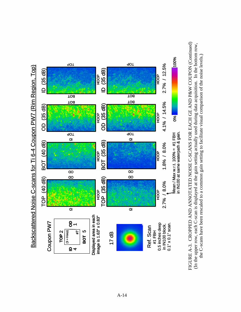
Bac

ksca

ttere

d N

oise

C-s

cans

for T

i 6-4

Cou

pon

PW7

(Rim

Reg

ion,

Top

)

TOP

(40

dB)

BO

T (4

0 dB

)O

D (

35 d

B)ID

(35

dB)

ODOD

ID

ID

TOP

TOP

BOT

BOT

HO

OP

HO

OP

HO

OP

HO

OP

TOP

(35

dB)

BO

T (3

5 dB

)O

D (

35 d

B)ID

(35

dB)

ODOD

ID

ID

TOP

TOP

BOT

BOT

HO

OP

HO

OP

HO

OP

HO

OP

0%10

0%

2.7%

/ 8

.0%

1.8%

/ 8

.0%

4.1%

/ 1

4.5%

2.7%

/ 1

2.5%

17 d

B#72

4

5

1

(3 =

Hoo

p)

TOP

BO

T

IDO

D

Dis

play

ed a

rea

in e

ach

imag

e is

1.6

3” x

0.8

3”

Cou

pon

PW7

Ref

. Sca

n#1

FBH

0.

5 in

ches

dee

pin

IN10

0 bl

ock.

0.1”

x 0

.1” s

can.

Mea

n / M

ax w

.r.t.

100%

= #

1 FB

Hin

IN10

0 at

sam

e w

ater

path

& g

ain.

Bac

ksca

ttere

d N

oise

C-s

cans

for T

i 6-4

Cou

pon

PW7

(Rim

Reg

ion,

Top

)

TOP

(40

dB)

BO

T (4

0 dB

)O

D (

35 d

B)ID

(35

dB)

ODOD

ID

ID

TOP

TOP

BOT

BOT

HO

OP

HO

OP

HO

OP

HO

OP

TOP

(35

dB)

BO

T (3

5 dB

)O

D (

35 d

B)ID

(35

dB)

ODOD

ID

ID

TOP

TOP

BOT

BOT

HO

OP

HO

OP

HO

OP

HO

OP

ODOD

ID

ID

TOP

TOP

BOT

BOT

HO

OP

HO

OP

HO

OP

HO

OP

TOP

(35

dB)

BO

T (3

5 dB

)O

D (

35 d

B)ID

(35

dB)

ODOD

ID

ID

TOP

TOP

BOT

BOT

HO

OP

HO

OP

HO

OP

HO

OP

0%10

0%0%

100%

2.7%

/ 8

.0%

1.8%

/ 8

.0%

4.1%

/ 1

4.5%

2.7%

/ 1

2.5%

17 d

B#72

4

5

1

(3 =

Hoo

p)

TOP

BO

T

IDO

D

Dis

play

ed a

rea

in e

ach

imag

e is

1.6

3” x

0.8

3”

Cou

pon

PW7

#72

4

5

1

(3 =

Hoo

p)

TOP

BO

T

IDO

D

Dis

play

ed a

rea

in e

ach

imag

e is

1.6

3” x

0.8

3”

Cou

pon

PW7

Ref

. Sca

n#1

FBH

0.

5 in

ches

dee

pin

IN10

0 bl

ock.

0.1”

x 0

.1” s

can.

Mea

n / M

ax w

.r.t.

100%

= #

1 FB

Hin

IN10

0 at

sam

e w

ater

path

& g

ain.

A-14

FI

GU

RE

A-3

. C

RO

PPED

AN

D A

NN

OTA

TED

NO

ISE

C-S

CA

NS

FOR

EA

CH

GE

AN

D P

&W

CO

UPO

N (C

ontin

ued)

(I

n th

e up

per r

ow, e

ach

C-s

can

is d

ispl

ayed

at t

he g

ain

setti

ng a

ctua

lly u

sed

durin

g da

ta a

cqui

sitio

n. I

n th

e bo

ttom

row

, th

e C

-sca

ns h

ave

been

resc

aled

to a

com

mon

gai

n se

tting

to fa

cilit

ate

visu

al c

ompa

rison

of t

he n

oise

leve

ls.)

Back

scat

tere

d N

oise

C-s

cans

for T

i 6-4

Cou

pon

PW8

(Rim

Reg

ion,

Cen

ter)

TOP

(42

dB

)B

OT

(42

dB)

OD

(35

dB

)ID

(33

dB

)

ODOD

ID

ID

TOP

TOP

BOT

BOT

HO

OP

HO

OP

HO

OP

HO

OP

TOP

(33

dB

)B

OT

(33

dB)

OD

(33

dB

)ID

(33

dB

)

ODOD

ID

ID

TOP

TOP

BOT

BOT

HO

OP

HO

OP

HO

OP

HO

OP

0%10

0%

1.6%

/ 5

.5%

1.5%

/ 4

.6%

5.0%

/ 1

4.4%

5.1%

/ 1

7.0%

17 d

B#82

4

5

1

(3 =

Hoo

p)

TOP

BO

T

IDO

D

Dis

play

ed a

rea

in e

ach

imag

e is

1.6

3” x

0.8

3”

Cou

pon

PW8

Ref

. Sca

n#1

FB

H

0.5

inch

es d

eep

in IN

100

bloc

k.0.

1” x

0.1

” sca

n.M

ean

/ Max

w.r.

t. 10

0% =

#1

FBH

in IN

100

at s

ame

wat

erpa

th &

gai

n.

Back

scat

tere

d N

oise

C-s

cans

for T

i 6-4

Cou

pon

PW8

(Rim

Reg

ion,

Cen

ter)

TOP

(42

dB

)B

OT

(42

dB)

OD

(35

dB

)ID

(33

dB

)

ODOD

ID

ID

TOP

TOP

BOT

BOT

HO

OP

HO

OP

HO

OP

HO

OP

TOP

(33

dB

)B

OT

(33

dB)

OD

(33

dB

)ID

(33

dB

)

ODOD

ID

ID

TOP

TOP

BOT

BOT

HO

OP

HO

OP

HO

OP

HO

OP

TOP

(42

dB

)B

OT

(42

dB)

OD

(35

dB

)ID

(33

dB

)

ODOD

ID

ID

TOP

TOP

BOT

BOT

HO

OP

HO

OP

HO

OP

HO

OP

TOP

(33

dB

)B

OT

(33

dB)

OD

(33

dB

)ID

(33

dB

)

ODOD

ID

ID

TOP

TOP

BOT

BOT

HO

OP

HO

OP

HO

OP

HO

OP

0%10

0%0%

100%

1.6%

/ 5

.5%

1.5%

/ 4

.6%

5.0%

/ 1

4.4%

5.1%

/ 1

7.0%

17 d

B#82

4

5

1

(3 =

Hoo

p)

TOP

BO

T

IDO

D

Dis

play

ed a

rea

in e

ach

imag

e is

1.6

3” x

0.8

3”

Cou

pon

PW8

#82

4

5

1

(3 =

Hoo

p)

TOP

BO

T

IDO

D

Dis

play

ed a

rea

in e

ach

imag

e is

1.6

3” x

0.8

3”

Cou

pon

PW8

Ref

. Sca

n#1

FB

H

0.5

inch

es d

eep

in IN

100

bloc

k.0.

1” x

0.1

” sca

n.M

ean

/ Max

w.r.

t. 10

0% =

#1

FBH

in IN

100

at s

ame

wat

erpa

th &

gai

n.

A-15

FI

GU

RE

A-3

. C

RO

PPED

AN

D A

NN

OTA

TED

NO

ISE

C-S

CA

NS

FOR

EA

CH

GE

AN

D P

&W

CO

UPO

N (C

ontin

ued)

(I

n th

e up

per r

ow, e

ach

C-s

can

is d

ispl

ayed

at t

he g

ain

setti

ng a

ctua

lly u

sed

durin

g da

ta a

cqui

sitio

n. I

n th

e bo

ttom

row

, th

e C

-sca

ns h

ave

been

resc

aled

to a

com

mon

gai

n se

tting

to fa

cilit

ate

visu

al c

ompa

rison

of t

he n

oise

leve

ls.)

Typi

cal N

oise

C-s

can:

Im

age

Labe

ls a

nd S

tatis

tics

for H

W C

oupo

ns

Tabl

e lis

ts a

vera

ge

and

max

imum

gate

d-pe

ak n

oise

am

plitu

de, a

s a

perc

enta

ge o

f the

am

plitu

de o

f the

#1

FBH

in IN

100

at

the

sam

e w

ater

pa

th a

nd g

ain.

Ampl

itude

s ar

e co

mpu

ted

for t

he

redu

ced-

area

re

gion

(illu

stra

ted

abov

e) w

ith “e

dge

effe

cts”

cro

pped

.Side 2 -AFT

Side 5 -FWD

(Sid

e 3

–ho

op)

Thru

OD

Insp

ectio

n en

try

surfa

ce

“Hoo

p” e

dge

(Sid

e 3)

is

alw

ays

at th

e bo

ttom

of t

he

imag

e,

allo

win

g th

e ot

her e

dges

to

be re

adily

id

entif

ied.

Spe

cim

en,

insp

ectio

n di

rect

ion

and

abso

lute

ga

in

setti

ng.Info

App

earin

g on

Sum

mar

y Fi

gure

s

Tic

mar

ks

are

0.5”

ap

art

H3

Side

1, 3

7dB

Avg

.: 2.

58%

2

.13%

3

.03%

Peak

: 10.

4%

6.1

1%

10.

4%

Full

imag

e

Left

half

Rig

ht

half

Cro

pped

re

gion

use

d fo

r noi

se

stat

istic

s

Reg

ion

scan

ned

mea

sure

s 1.

6” w

ide

by 2

.5” t

all i

n st

eps

of 0

.02”

. N

ear t

he b

ound

arie

s of

the

spec

imen

, the

noi

se a

mpl

itude

s ar

e af

fect

ed b

y “e

dge

effe

cts”

.“Raw

” C-s

can

for

HW

Cou

pon

#3 (A

FT/O

D re

gion

) In

spec

ted

thru

OD

sur

face

0%10

0%

Typi

cal N

oise

C-s

can:

Im

age

Labe

ls a

nd S

tatis

tics

for H

W C

oupo

ns

Tabl

e lis

ts a

vera

ge

and

max

imum

gate

d-pe

ak n

oise

am

plitu

de, a

s a

perc

enta

ge o

f the

am

plitu

de o

f the

#1

FBH

in IN

100

at

the

sam

e w

ater

pa

th a

nd g

ain.

Ampl

itude

s ar

e co

mpu

ted

for t

he

redu

ced-

area

re

gion

(illu

stra

ted

abov

e) w

ith “e

dge

effe

cts”

cro

pped

.Side 2 -AFT

Side 5 -FWD

(Sid

e 3

–ho

op)

Thru

OD

Insp

ectio

n en

try

surfa

ce

“Hoo

p” e

dge

(Sid

e 3)

is

alw

ays

at th

e bo

ttom

of t

he

imag

e,

allo

win

g th

e ot

her e

dges

to

be re

adily

id

entif

ied.

Spe

cim

en,

insp

ectio

n di

rect

ion

and

abso

lute

ga

in

setti

ng.Info

App

earin

g on

Sum

mar

y Fi

gure

s

Tic

mar

ks

are

0.5”

ap

art

H3

Side

1, 3

7dB

Avg

.: 2.

58%

2

.13%

3

.03%

Peak

: 10.

4%

6.1

1%

10.

4%

Full

imag

e

Left

half

Rig

ht

half

Cro

pped

re

gion

use

d fo

r noi

se

stat

istic

sTa

ble

lists

ave

rage

an

d m

axim

umga

ted-

peak

noi

se

ampl

itude

, as

a pe

rcen

tage

of t

he

ampl

itude

of t

he #

1 FB

H in

IN10

0 at

th

e sa

me

wat

er

path

and

gai

n.

Ampl

itude

s ar

e co

mpu

ted

for t

he

redu

ced-

area

re

gion

(illu

stra

ted

abov

e) w

ith “e

dge

effe

cts”

cro

pped

.Side 2 -AFT

Side 5 -FWD

(Sid

e 3

–ho

op)

Thru

OD

Insp

ectio

n en

try

surfa

ce

“Hoo

p” e

dge

(Sid

e 3)

is

alw

ays

at th

e bo

ttom

of t

he

imag

e,

allo

win

g th

e ot

her e

dges

to

be re

adily

id

entif

ied.

Spe

cim

en,

insp

ectio

n di

rect

ion

and

abso

lute

ga

in

setti

ng.Info

App

earin

g on

Sum

mar

y Fi

gure

s

Tic

mar

ks

are

0.5”

ap

art

H3

Side

1, 3

7dB

Avg

.: 2.

58%

2

.13%

3

.03%

Peak

: 10.

4%

6.1

1%

10.

4%

Full

imag

e

Left

half

Rig

ht

half

H3

Side

1, 3

7dB

Avg

.: 2.

58%

2

.13%

3

.03%

Peak

: 10.

4%

6.1

1%

10.

4%

Full

imag

e

Left

half

Rig

ht

half

H3

Side

1, 3

7dB

Avg

.: 2.

58%

2

.13%

3

.03%

Peak

: 10.

4%

6.1

1%

10.

4%

Full

imag

e

Left

half

Rig

ht

half

Avg

.: 2.

58%

2

.13%

3

.03%

Peak

: 10.

4%

6.1

1%

10.

4%

Full

imag

e

Left

half

Rig

ht

half

Cro

pped

re

gion

use

d fo

r noi

se

stat

istic

s

Reg

ion

scan

ned

mea

sure

s 1.

6” w

ide

by 2

.5” t

all i

n st

eps

of 0

.02”

. N

ear t

he b

ound

arie

s of

the

spec

imen

, the

noi

se a

mpl

itude

s ar

e af

fect

ed b

y “e

dge

effe

cts”

.“Raw

” C-s

can

for

HW

Cou

pon

#3 (A

FT/O

D re

gion

) In

spec

ted

thru

OD

sur

face

0%10

0%

Reg

ion

scan

ned

mea

sure

s 1.

6” w

ide

by 2

.5” t

all i

n st

eps

of 0

.02”

. N

ear t

he b

ound

arie

s of

the

spec

imen

, the

noi

se a

mpl

itude

s ar

e af

fect

ed b

y “e

dge

effe

cts”

.“Raw

” C-s

can

for

HW

Cou

pon

#3 (A

FT/O

D re

gion

) In

spec

ted

thru

OD

sur

face

0%10

0%0%

100%

A-16

FI

GU

RE

A-4

. EX

PLA

NA

TIO

N O

F LA

BEL

ING

CO

NV

ENTI

ON

S FO

R N

OIS

E C

-SC

AN

S O

F TH

E H

W

FOR

GIN

G L

OW

LIN

E C

OU

PON

S

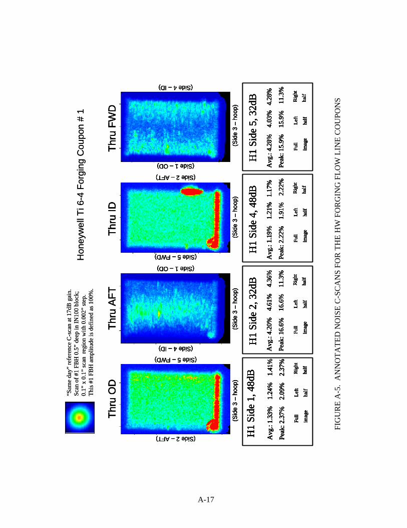
A-17

H1

Side

1, 4

8dB

Avg

.: 1.

33%

1

.24%

1

.41%

Peak

: 2.3

7%

2.0

9%

2.3

7%

Full

imag

e

Left

half

Rig

ht

half

H1

Side

2, 3

2dB

Avg

.: 4.

20%

4

.61%

4

.36%

(Side 2 –AFT)

Thru

OD

Thru

FW

DTh

ru A

FTTh

ru ID

(Sid

e 3

–ho

op)

(Sid

e 3

–ho

op)

(Sid

e 3

–ho

op)

(Sid

e 3

–ho

op)

(Side 2 –AFT)

(Side 5 –FWD)

(Side 5 –FWD)

(Side 4 –ID)

(Side 1 –OD)

(Side 4 –ID)

(Side 1 –OD)

Hon

eyw

ell T

i 6-4

For

ging

Cou

pon

# 1

FI

GU

RE

A-5

. A

NN

OTA

TED

NO

ISE

C-S

CA

NS

FOR

TH

E H

W F

OR

GIN

G F

LOW

LIN

E C

OU

PON

S

Peak

: 16.

6%

16.

6%

11.

3%

Full

imag

e

Left

half

Rig

ht

half

H1

Side

4, 4

8dB

Avg

.: 1.

19%

1

.21%

1.

17%

Peak

: 2.2

2%

1.9

1%

2.2

2%

Full

imag

e

Left

half

Rig

ht

half

H1

Side

5, 3

2dB

Avg

.: 4.

28%

4

.03%

4.

28%

Peak

: 15.

9%

15.

9%

11.

3%

Full

imag

e

Left

half

Rig

ht

half

“Sam

e da

y” re

fere

nce

C-s

can

at 1

7dB

gai

n.

Scan

of #

1 FB

H 0

.5”

deep

in IN

100

bloc

k;

0.1”

x 0

.1”

scan

reg

ion

with

0.0

02”

step

. Th

is #

1 FB

H a

mpl

itude

is d

efin

ed a

s 100

%.

(Side 2 –AFT)

Thru

OD

Thru

FW

DTh

ru A

FTTh

ru ID

(Sid

e 3

–ho

op)

(Sid

e 3

–ho

op)

(Sid

e 3

–ho

op)

(Sid

e 3

–ho

op)

(Side 2 –AFT)

(Side 5 –FWD)

(Side 5 –FWD)

(Side 4 –ID)

(Side 1 –OD)

(Side 4 –ID)

(Side 1 –OD)

(Side 2 –AFT)

Thru

OD

Thru

FW

DTh

ru A

FTTh

ru ID

(Sid

e 3

–ho

op)

(Sid

e 3

–ho

op)

(Sid

e 3

–ho

op)

(Sid

e 3

–ho

op)

(Side 2 –AFT)

(Side 5 –FWD)

(Side 5 –FWD)

(Side 4 –ID)

(Side 1 –OD)

(Side 4 –ID)

(Side 1 –OD)

Thru

OD

Thru

FW

DTh

ru A

FTTh

ru ID

(Sid

e 3

–ho

op)

(Sid

e 3

–ho

op)

(Sid

e 3

–ho

op)

(Sid

e 3

–ho

op)

(Side 2 –AFT)

(Side 5 –FWD)

(Side 5 –FWD)

(Side 4 –ID)

(Side 1 –OD)

(Side 4 –ID)

(Side 1 –OD)

Hon

eyw

ell T

i 6-4

For

ging

Cou

pon

# 1

“Sam

e da

y” re

fere

nce

C-s

can

at 1

7dB

gai

n.

Scan

of #

1 FB

H 0

.5”

deep

in IN

100

bloc

k;

0.1”

x 0

.1”

scan

reg

ion

with

0.0

02”

step

. Th

is #

1 FB

H a

mpl

itude

is d

efin

ed a

s 100

%.

H1

Side

1, 4

8dB

Avg

.: 1.

33%

1

.24%

1

.41%

Peak

: 2.3

7%

2.0

9%

2.3

7%

Full

imag

e

Left

half

Rig

ht

half

H1

Side

2, 3

2dB

Avg

.: 4.

20%

4

.61%

4

.36%

Peak

: 16.

6%

16.

6%

11.

3%

Full

imag

e

Left

half

Rig

ht

half

H1

Side

4, 4

8dB

Avg

.: 1.

19%

1

.21%

1.

17%

Peak

: 2.2

2%

1.9

1%

2.2

2%

Full

imag

e

Left

half

Rig

ht

half

H1

Side

5, 3

2dB

Avg

.: 4.

28%

4

.03%

4.

28%

Peak

: 15.

9%

15.

9%

11.

3%

Full

imag

e

Left

half

Rig

ht

half

H1

Side

1, 4

8dB

Avg

.: 1.

33%

1

.24%

1

.41%

Peak

: 2.3

7%

2.0

9%

2.3

7%

Full

imag

e

Left

half

Rig

ht

half

H1

Side

1, 4

8dB

Avg

.: 1.

33%

1

.24%

1

.41%

Peak

: 2.3

7%

2.0

9%

2.3

7%

Full

imag

e

Left

half

Rig

ht

half

H1

Side

1, 4

8dB

Avg

.: 1.

33%

1

.24%

1

.41%

Peak

: 2.3

7%

2.0

9%

2.3

7%

Full

imag

e

Left

half

Rig

ht

half

Avg

.: 1.

33%

1

.24%

1

.41%

Peak

: 2.3

7%

2.0

9%

2.3

7%

Full

imag

e

Left

half

Rig

ht

half

H1

Side

2, 3

2dB

Avg

.: 4.

20%

4

.61%

4

.36%

Peak

: 16.

6%

16.

6%

11.

3%

Full

imag

e

Left

half

Rig

ht

half

H1

Side

2, 3

2dB

Avg

.: 4.

20%

4

.61%

4

.36%

Peak

: 16.

6%

16.

6%

11.

3%

Full

imag

e

Left

half

Rig

ht

half

H1

Side

2, 3

2dB

Avg

.: 4.

20%

4

.61%

4

.36%

Peak

: 16.

6%

16.

6%

11.

3%

Full

imag

e

Left

half

Rig

ht

half

Avg

.: 4.

20%

4

.61%

4

.36%

Peak

: 16.

6%

16.

6%

11.

3%

Full

imag

e

Left

half

Rig

ht

half

H1

Side

4, 4

8dB

Avg

.: 1.

19%

1

.21%

1.

17%

Peak

: 2.2

2%

1.9

1%

2.2

2%

Full

imag

e

Left

half

Rig

ht

half

H1

Side

4, 4

8dB

Avg

.: 1.

19%

1

.21%

1.

17%

Peak

: 2.2

2%

1.9

1%

2.2

2%

Full

imag

e

Left

half

Rig

ht

half

H1

Side

4, 4

8dB

Avg

.: 1.

19%

1

.21%

1.

17%

Peak

: 2.2

2%

1.9

1%

2.2

2%

Full

imag

e

Left

half

Rig

ht

half

Avg

.: 1.

19%

1

.21%

1.

17%

Peak

: 2.2

2%

1.9

1%

2.2

2%

Full

imag

e

Left

half

Rig

ht

half

H1

Side

5, 3

2dB

Avg

.: 4.

28%

4

.03%

4.

28%

Peak

: 15.

9%

15.

9%

11.

3%

Full

imag

e

Left

half

Rig

ht

half

H1

Side

5, 3

2dB

Avg

.: 4.

28%

4

.03%

4.

28%

Peak

: 15.

9%

15.

9%

11.

3%

Full

imag

e

Left

half

Rig

ht

half

H1

Side

5, 3

2dB

Avg

.: 4.

28%

4

.03%

4.

28%

Peak

: 15.

9%

15.

9%

11.

3%

Full

imag

e

Left

half

Rig

ht

half

Avg

.: 4.

28%

4

.03%

4.

28%

Peak

: 15.

9%

15.

9%

11.

3%

Full

imag

e

Left

half

Rig

ht

half

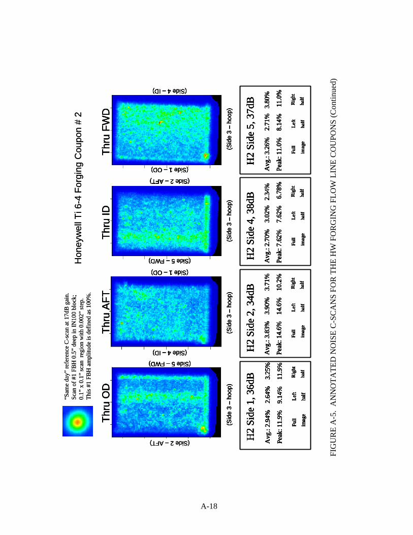
A-18

H2

Side

1, 3

6dB

Avg

.: 2.

94%

2

.64%

3

.25%

Peak

: 11.

9%

9.1

4%

11.

9%

Full

imag

e

Left

half

Rig

ht

half

H2

Side

2, 3

4dB

Avg

.: 3.

83%

3

.90%

3

.71%

Peak

: 14.

6%

14.

6%

10.

2%

Full

imag

e

Left

half

Rig

ht

half

H2

Side

4, 3

8dB

Avg

.: 2.

70%

3

.02%

2.

34%

Peak

: 7.6

2%

7.6

2%

6.7

8%

Full

imag

e

Left

half

Rig

ht

half

H2

Side

5, 3

7dB

Avg

.: 3.

26%

2

.71%

3.

80%

Peak

: 11.

0%

8.1

4%

11.

0%

Full

imag

e

Left

half

Rig

ht

half

(Side 2 –AFT)

Thru

OD

Thru

FW

DTh

ru A

FTTh

ru ID

(Sid

e 3

–ho

op)

(Sid

e 3

–ho

op)

(Sid

e 3

–ho

op)

(Sid

e 3

–ho

op)

(Side 2 –AFT)

(Side 5 –FWD)

(Side 5 –FWD)

(Side 4 –ID)

(Side 1 –OD)

(Side 4 –ID)

(Side 1 –OD)

“Sam

e da

y” re

fere

nce

C-s

can

at 1

7dB

gai

n.

Scan

of #

1 FB

H 0

.5”

deep

in IN

100

bloc

k;

0.1”

x 0

.1”

scan

reg

ion

with

0.0

02”

step

. Th

is #

1 FB

H a

mpl

itude

is d

efin

ed a

s 100

%.

Hon

eyw

ell T

i 6-4

For

ging

Cou

pon

# 2

H2

Side

1, 3

6dB

Avg

.: 2.

94%

2

.64%

3

.25%

Peak

: 11.

9%

9.1

4%

11.

9%

Full

imag

e

Left

half

Rig

ht

half

H2

Side

2, 3

4dB

Avg

.: 3.

83%

3

.90%

3

.71%

Peak

: 14.

6%

14.

6%

10.

2%

Full

imag

e

Left

half

Rig

ht

half

H2

Side

4, 3

8dB

Avg

.: 2.

70%

3

.02%

2.

34%

Peak

: 7.6

2%

7.6

2%

6.7

8%

Full

imag

e

Left

half

Rig

ht

half

H2

Side

5, 3

7dB

Avg

.: 3.

26%

2

.71%

3.

80%

Peak

: 11.

0%

8.1

4%

11.

0%

Full

imag

e

Left

half

Rig

ht

half

H2

Side

1, 3

6dB

Avg

.: 2.

94%

2

.64%

3

.25%

Peak

: 11.

9%

9.1

4%

11.

9%

Full

imag

e

Left

half

Rig

ht

half

H2

Side

1, 3

6dB

Avg

.: 2.

94%

2

.64%

3

.25%

Peak

: 11.

9%

9.1

4%

11.

9%

Full

imag

e

Left

half

Rig

ht

half

H2

Side

1, 3

6dB

Avg

.: 2.

94%

2

.64%

3

.25%

Peak

: 11.

9%

9.1

4%

11.

9%

Full

imag

e

Left

half

Rig

ht

half

Avg

.: 2.

94%

2

.64%

3

.25%

Peak

: 11.

9%

9.1

4%

11.

9%

Full

imag

e

Left

half

Rig

ht

half

H2

Side

2, 3

4dB

Avg

.: 3.

83%

3

.90%

3

.71%

Peak

: 14.

6%

14.

6%

10.

2%

Full

imag

e

Left

half

Rig

ht

half

H2

Side

2, 3

4dB

Avg

.: 3.

83%

3

.90%

3

.71%

Peak

: 14.

6%

14.

6%

10.

2%

Full

imag

e

Left

half

Rig

ht

half

H2

Side

2, 3

4dB

Avg

.: 3.

83%

3

.90%

3

.71%

Peak

: 14.

6%

14.

6%

10.

2%

Full

imag

e

Left

half

Rig

ht

half

Avg

.: 3.

83%

3

.90%

3

.71%

Peak

: 14.

6%

14.

6%

10.

2%

Full

imag

e

Left

half

Rig

ht

half

H2

Side

4, 3

8dB

Avg

.: 2.

70%

3

.02%

2.

34%

Peak

: 7.6

2%

7.6

2%

6.7

8%

Full

imag

e

Left

half

Rig

ht

half

H2

Side

4, 3

8dB

Avg

.: 2.

70%

3

.02%

2.

34%

Peak

: 7.6

2%

7.6

2%

6.7

8%

Full

imag

e

Left

half

Rig

ht

half

H2

Side

4, 3

8dB

Avg

.: 2.

70%

3

.02%

2.

34%

Peak

: 7.6

2%

7.6

2%

6.7

8%

Full

imag

e

Left

half

Rig

ht

half

Avg

.: 2.

70%

3

.02%

2.

34%

Peak

: 7.6

2%

7.6

2%

6.7

8%

Full

imag

e

Left

half

Rig

ht

half

H2

Side

5, 3

7dB

Avg

.: 3.

26%

2

.71%

3.

80%

Peak

: 11.

0%

8.1

4%

11.

0%

Full

imag

e

Left

half

Rig

ht

half

H2

Side

5, 3

7dB

Avg

.: 3.

26%

2

.71%

3.

80%

Peak

: 11.

0%

8.1

4%

11.

0%

Full

imag

e

Left

half

Rig

ht

half

H2

Side

5, 3

7dB

Avg

.: 3.

26%

2

.71%

3.

80%

Peak

: 11.

0%

8.1

4%

11.

0%

Full

imag

e

Left

half

Rig

ht

half

Avg

.: 3.

26%

2

.71%

3.

80%

Peak

: 11.

0%

8.1

4%

11.

0%

Full

imag

e

Left

half

Rig

ht

half

(Side 2 –AFT)

Thru

OD

Thru

FW

DTh

ru A

FTTh

ru ID

(Sid

e 3

–ho

op)

(Sid

e 3

–ho

op)

(Sid

e 3

–ho

op)

(Sid

e 3

–ho

op)

(Side 2 –AFT)

(Side 5 –FWD)

(Side 5 –FWD)

(Side 4 –ID)

(Side 1 –OD)

(Side 4 –ID)

(Side 1 –OD)

(Side 2 –AFT)

Thru

OD

Thru

FW

DTh

ru A

FTTh

ru ID

(Sid

e 3

–ho

op)

(Sid

e 3

–ho

op)

(Sid

e 3

–ho

op)

(Sid

e 3

–ho

op)

(Side 2 –AFT)

(Side 5 –FWD)

(Side 5 –FWD)

(Side 4 –ID)

(Side 1 –OD)

(Side 4 –ID)

(Side 1 –OD)

Thru

OD

Thru

FW

DTh

ru A

FTTh

ru ID

(Sid

e 3

–ho

op)

(Sid

e 3

–ho

op)

(Sid

e 3

–ho

op)

(Sid

e 3

–ho

op)

(Side 2 –AFT)

(Side 5 –FWD)

(Side 5 –FWD)

(Side 4 –ID)

(Side 1 –OD)

(Side 4 –ID)

(Side 1 –OD)

“Sam

e da

y” re

fere

nce

C-s

can

at 1

7dB

gai

n.

Scan

of #

1 FB

H 0

.5”

deep

in IN

100

bloc

k;

0.1”

x 0

.1”

scan

reg

ion

with

0.0

02”

step

. Th

is #

1 FB

H a

mpl

itude

is d

efin

ed a

s 100

%.

Hon

eyw

ell T

i 6-4

For

ging

Cou

pon

# 2

FI

GU

RE

A-5

. A

NN

OTA

TED

NO

ISE

C-S

CA

NS

FOR

TH

E H

W F

OR

GIN

G F

LOW

LIN

E C

OU

PON

S (C

ontin

ued)

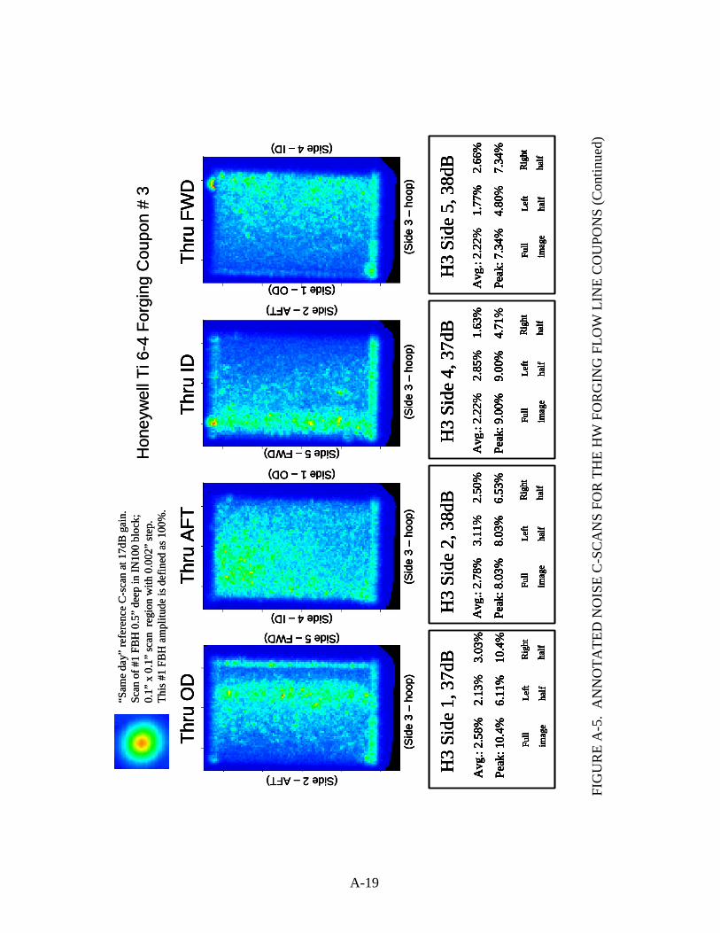
A-19

H3

Side

1, 3

7dB

Avg

.: 2.

58%

2

.13%

3

.03%

Peak

: 10.

4%

6.1

1%

10.

4%

Full

imag

e

Left

half

Rig

ht

half

H3

Side

2, 3

8dB

Avg

.: 2.

78%

3

.11%

2

.50%

Peak

: 8.0

3%

8.0

3%

6.5

3%

Full

imag

e

Left

half

Rig

ht

half

H3

Side

4, 3

7dB

Avg

.: 2.

22%

2

.85%

1

.63%

Peak

: 9.0

0%

9.0

0%

4.7

1%

Full

imag

e

Left

half

Rig

ht

half

H3

Side

5, 3

8dB

Avg

.: 2.

22%

1

.77%

2

.66%

Peak

: 7.3

4%

4.8

0%

7.3

4%

Full

imag

e

Left

half

Rig

ht

half

(Side 2 –AFT)

Thru

OD

Thru

FW

DTh

ru A

FTTh

ru ID

(Sid

e 3

–ho

op)

(Sid

e 3

–ho

op)

(Sid

e 3

–ho

op)

(Sid

e 3

–ho

op)

(Side 2 –AFT)

(Side 5 –FWD)

(Side 5 –FWD)

(Side 4 –ID)

(Side 1 –OD)

(Side 4 –ID)

(Side 1 –OD)

Hon

eyw

ell T

i 6-4

For

ging

Cou

pon

# 3

“Sam

e da

y” re

fere

nce

C-s

can

at 1

7dB

gain

. Sc

an o

f #1

FBH

0.5

” de

ep in

IN10

0 bl

ock;

0.

1” x

0.1

” sc

an r

egio

n w

ith 0

.002

” st

ep.

This

#1

FBH

am

plitu

de is

def

ined

as 1

00%

.

H3

Side

1, 3

7dB

Avg

.: 2.

58%

2

.13%

3

.03%

Peak

: 10.

4%

6.1

1%

10.

4%

Full

imag

e

Left

half

Rig

ht

half

H3

Side

2, 3

8dB

Avg

.: 2.

78%

3

.11%

2

.50%

Peak

: 8.0

3%

8.0

3%

6.5

3%

Full

imag

e

Left

half

Rig

ht

half

H3

Side

4, 3

7dB

Avg

.: 2.

22%

2

.85%

1

.63%

Peak

: 9.0

0%

9.0

0%

4.7

1%

Full

imag

e

Left

half

Rig

ht

half

H3

Side

5, 3

8dB

Avg

.: 2.

22%

1

.77%

2

.66%

Peak

: 7.3

4%

4.8

0%

7.3

4%

Full

imag

e

Left

half

Rig

ht

half

H3

Side

1, 3

7dB

Avg

.: 2.

58%

2

.13%

3

.03%

Peak

: 10.

4%

6.1

1%

10.

4%

Full

imag

e

Left

half

Rig

ht

half

H3

Side

1, 3

7dB

Avg

.: 2.

58%

2

.13%

3

.03%

Peak

: 10.

4%

6.1

1%

10.

4%

Full

imag

e

Left

half

Rig

ht

half

H3

Side

1, 3

7dB

Avg

.: 2.

58%

2

.13%

3

.03%

Peak

: 10.

4%

6.1

1%

10.

4%

Full

imag

e

Left

half

Rig

ht

half

Avg

.: 2.

58%

2

.13%

3

.03%

Peak

: 10.

4%

6.1

1%

10.

4%

Full

imag

e

Left

half

Rig

ht

half

H3

Side

2, 3

8dB

Avg

.: 2.

78%

3

.11%

2

.50%

Peak

: 8.0

3%

8.0

3%

6.5

3%

Full

imag

e

Left

half

Rig

ht

half

H3

Side

2, 3

8dB

Avg

.: 2.

78%

3

.11%

2

.50%

Peak

: 8.0

3%

8.0

3%

6.5

3%

Full

imag

e

Left

half

Rig

ht

half

H3

Side

2, 3

8dB

Avg

.: 2.

78%

3

.11%

2

.50%

Peak

: 8.0

3%

8.0

3%

6.5

3%

Full

imag

e

Left

half

Rig

ht

half

Avg

.: 2.

78%

3

.11%

2

.50%

Peak

: 8.0

3%

8.0

3%

6.5

3%

Full

imag

e

Left

half

Rig

ht

half

H3

Side

4, 3

7dB

Avg

.: 2.

22%

2

.85%

1

.63%

Peak

: 9.0

0%

9.0

0%

4.7

1%

Full

imag

e

Left

half

Rig

ht

half

H3

Side

4, 3

7dB

Avg

.: 2.

22%

2

.85%

1

.63%

Peak

: 9.0

0%

9.0

0%

4.7

1%

Full

imag

e

Left

half

Rig

ht

half

H3

Side

4, 3

7dB

Avg

.: 2.

22%

2

.85%

1

.63%

Peak

: 9.0

0%

9.0

0%

4.7

1%

Full

imag

e

Left

half

Rig

ht

half

Avg

.: 2.

22%

2

.85%

1

.63%

Peak

: 9.0

0%

9.0

0%

4.7

1%

Full

imag

e

Left

half

Rig

ht

half

H3

Side

5, 3

8dB

Avg

.: 2.

22%

1

.77%

2

.66%

Peak

: 7.3

4%

4.8

0%

7.3

4%

Full

imag

e

Left

half

Rig

ht

half

H3

Side

5, 3

8dB

Avg

.: 2.

22%

1

.77%

2

.66%

Peak

: 7.3

4%

4.8

0%

7.3

4%

Full

imag

e

Left

half

Rig

ht

half

H3

Side

5, 3

8dB

Avg

.: 2.

22%

1

.77%

2

.66%

Peak

: 7.3

4%

4.8

0%

7.3

4%

Full

imag

e

Left

half

Rig

ht

half

Avg

.: 2.

22%

1

.77%

2

.66%

Peak

: 7.3

4%

4.8

0%

7.3

4%

Full

imag

e

Left

half

Rig

ht

half

(Side 2 –AFT)

Thru

OD

Thru

FW

DTh

ru A

FTTh

ru ID

(Sid

e 3

–ho

op)

(Sid

e 3

–ho

op)

(Sid

e 3

–ho

op)

(Sid

e 3

–ho

op)

(Side 2 –AFT)

(Side 5 –FWD)

(Side 5 –FWD)

(Side 4 –ID)

(Side 1 –OD)

(Side 4 –ID)

(Side 1 –OD)

(Side 2 –AFT)

Thru

OD

Thru

FW

DTh

ru A

FTTh

ru ID

(Sid

e 3

–ho

op)

(Sid

e 3

–ho

op)

(Sid

e 3

–ho

op)

(Sid

e 3

–ho

op)

(Side 2 –AFT)

(Side 5 –FWD)

(Side 5 –FWD)

(Side 4 –ID)

(Side 1 –OD)

(Side 4 –ID)

(Side 1 –OD)

Thru

OD

Thru

FW

DTh

ru A

FTTh

ru ID

(Sid

e 3

–ho

op)

(Sid

e 3

–ho

op)

(Sid

e 3

–ho

op)

(Sid

e 3

–ho

op)

(Side 2 –AFT)

(Side 5 –FWD)

(Side 5 –FWD)

(Side 4 –ID)

(Side 1 –OD)

(Side 4 –ID)

(Side 1 –OD)

Hon

eyw

ell T

i 6-4

For

ging

Cou

pon

# 3

“Sam

e da

y” re

fere

nce

C-s

can

at 1

7dB

gain

. Sc

an o

f #1

FBH

0.5

” de

ep in

IN10

0 bl

ock;

0.

1” x

0.1

” sc

an r

egio

n w

ith 0

.002

” st

ep.

This

#1

FBH

am

plitu

de is

def

ined

as 1

00%

.

FI

GU

RE

A-5

. A

NN

OTA

TED

NO

ISE

C-S

CA

NS

FOR

TH

E H

W F

OR

GIN

G F

LOW

LIN

E C

OU

PON

S (C

ontin

ued)

A-20

H4

Side

1, 3

9dB

Avg

.: 2.

52%

2

.59%

2

.52%

Peak

: 8.8

4%

8.8

4%

6.6

9%

Full

imag

e

Left

half

Rig

ht

half

H4

Side

2, 3

5dB

Avg

.: 4.

61%

4

.50%

4

.73%

Peak

: 13.

0%

11.

5%

13.

0%

Full

imag

e

Left

half

Rig

ht

half

H4

Side

4, 3

8dB

Avg

.: 2.

06%

2

.18%

1.

94%

Peak

: 7.7

8%

5.7

7%

7.7

8%

Full

imag

e

Left

half

Rig

ht

half

H4

Side

5, 3

5dB

Avg

.: 2.

91%

2

.62%

3.

13%

Peak

: 11.

3%

7.8

0%

11.3

%

Full

imag

e

Left

half

Rig

ht

half

(Side 2 –AFT)Th

ru O

DTh

ru F

WD

Thru

AFT

Thru

ID

(Sid

e 3

–ho

op)

(Sid

e 3

–ho

op)

(Sid

e 3

–ho

op)

(Sid

e 3

–ho

op)

(Side 2 –AFT)

(Side 5 –FWD)

(Side 5 –FWD)

(Side 4 –ID)

(Side 1 –OD)

(Side 4 –ID)

(Side 1 –OD)

Hon

eyw

ell T

i 6-4

For

ging

Cou

pon

# 4

“Sam

e da

y” re

fere

nce

C-s

can

at 1

7dB

gain

. Sc

an o

f #1

FBH

0.5

” de

ep in

IN10

0 bl

ock;

0.

1” x

0.1

” sc

an r

egio

n w

ith 0

.002

” st

ep.

This

#1

FBH

am

plitu

de is

def

ined

as 1

00%

.

H4

Side

1, 3

9dB

Avg

.: 2.

52%

2

.59%

2

.52%

Peak

: 8.8

4%

8.8

4%

6.6

9%

Full

imag

e

Left

half

Rig

ht

half

H4

Side

2, 3

5dB

Avg

.: 4.

61%

4

.50%

4

.73%

Peak

: 13.

0%

11.

5%

13.

0%

Full

imag

e

Left

half

Rig

ht

half

H4

Side

4, 3

8dB

Avg

.: 2.

06%

2

.18%

1.

94%

Peak

: 7.7

8%

5.7

7%

7.7

8%

Full

imag

e

Left

half

Rig

ht

half

H4

Side

5, 3

5dB

Avg

.: 2.

91%

2

.62%

3.

13%

Peak

: 11.

3%

7.8

0%

11.3

%

Full

imag

e

Left

half

Rig

ht

half

H4

Side

1, 3

9dB

Avg

.: 2.

52%

2

.59%

2

.52%

Peak

: 8.8

4%

8.8

4%

6.6

9%

Full

imag

e

Left

half

Rig

ht

half

H4

Side

1, 3

9dB

Avg

.: 2.

52%

2

.59%

2

.52%

Peak

: 8.8

4%

8.8

4%

6.6

9%

Full

imag

e

Left

half

Rig

ht

half

H4

Side

1, 3

9dB

Avg

.: 2.

52%

2

.59%

2

.52%

Peak

: 8.8

4%

8.8

4%

6.6

9%

Full

imag

e

Left

half

Rig

ht

half

Avg

.: 2.

52%

2

.59%

2

.52%

Peak

: 8.8

4%

8.8

4%

6.6

9%

Full

imag

e

Left

half

Rig

ht

half

H4

Side

2, 3

5dB

Avg

.: 4.

61%

4

.50%

4

.73%

Peak

: 13.

0%

11.

5%

13.

0%

Full

imag

e

Left

half

Rig

ht

half

H4

Side

2, 3

5dB

Avg

.: 4.

61%

4

.50%

4

.73%

Peak

: 13.

0%

11.

5%

13.

0%

Full

imag

e

Left

half

Rig

ht

half

H4

Side

2, 3

5dB

Avg

.: 4.

61%

4

.50%

4

.73%

Peak

: 13.

0%

11.

5%

13.

0%

Full

imag

e

Left

half

Rig

ht

half

Avg

.: 4.

61%

4

.50%

4

.73%

Peak

: 13.

0%

11.

5%

13.

0%

Full

imag

e

Left

half

Rig

ht

half

H4

Side

4, 3

8dB

Avg

.: 2.

06%

2

.18%

1.

94%

Peak

: 7.7

8%

5.7

7%

7.7

8%

Full

imag

e

Left

half

Rig

ht

half

H4

Side

4, 3

8dB

Avg

.: 2.

06%

2

.18%

1.

94%

Peak

: 7.7

8%

5.7

7%

7.7

8%

Full

imag

e

Left

half

Rig

ht

half

H4

Side

4, 3

8dB

Avg

.: 2.

06%

2

.18%

1.

94%

Peak

: 7.7

8%

5.7

7%

7.7

8%

Full

imag

e

Left

half

Rig

ht

half

Avg

.: 2.

06%

2

.18%

1.

94%

Peak

: 7.7

8%

5.7

7%

7.7

8%

Full

imag

e

Left

half

Rig

ht

half

H4

Side

5, 3

5dB

Avg

.: 2.

91%

2

.62%

3.

13%

Peak

: 11.

3%

7.8

0%

11.3

%

Full

imag

e

Left

half

Rig

ht

half

H4

Side

5, 3

5dB

Avg

.: 2.

91%

2

.62%

3.

13%

Peak

: 11.

3%

7.8

0%

11.3

%

Full

imag

e

Left

half

Rig

ht

half

H4

Side

5, 3

5dB

Avg

.: 2.

91%

2

.62%

3.

13%

Peak

: 11.

3%

7.8

0%

11.3

%

Full

imag

e

Left

half

Rig

ht

half

Avg

.: 2.

91%

2

.62%

3.

13%

Peak

: 11.

3%

7.8

0%

11.3

%

Full

imag

e

Left

half

Rig

ht

half

(Side 2 –AFT)Th

ru O

DTh

ru F

WD

Thru

AFT

Thru

ID

(Sid

e 3

–ho

op)

(Sid

e 3

–ho

op)

(Sid

e 3

–ho

op)

(Sid

e 3

–ho

op)

(Side 2 –AFT)

(Side 5 –FWD)

(Side 5 –FWD)

(Side 4 –ID)

(Side 1 –OD)

(Side 4 –ID)

(Side 1 –OD)

(Side 2 –AFT)Th

ru O

DTh

ru F

WD

Thru

AFT

Thru

ID

(Sid

e 3

–ho

op)

(Sid

e 3

–ho

op)

(Sid

e 3

–ho

op)

(Sid

e 3

–ho

op)

(Side 2 –AFT)

(Side 5 –FWD)

(Side 5 –FWD)

(Side 4 –ID)

(Side 1 –OD)

(Side 4 –ID)

(Side 1 –OD)

Thru

OD

Thru

FW

DTh

ru A

FTTh

ru ID

(Sid

e 3

–ho

op)

(Sid

e 3

–ho

op)

(Sid

e 3

–ho

op)

(Sid

e 3

–ho

op)

(Side 2 –AFT)

(Side 5 –FWD)

(Side 5 –FWD)

(Side 4 –ID)

(Side 1 –OD)

(Side 4 –ID)

(Side 1 –OD)

Hon

eyw

ell T

i 6-4

For

ging

Cou

pon

# 4

“Sam

e da

y” re

fere

nce

C-s

can

at 1

7dB

gain

. Sc

an o

f #1

FBH

0.5

” de

ep in

IN10

0 bl

ock;

0.

1” x

0.1

” sc

an r

egio

n w

ith 0

.002

” st

ep.

This

#1

FBH

am

plitu

de is

def

ined

as 1

00%

.

FI

GU

RE

A-5

. A

NN

OTA

TED

NO

ISE

C-S

CA

NS

FOR

TH

E H

W F

OR

GIN

G F

LOW

LIN

E C

OU

PON

S (C

ontin

ued)

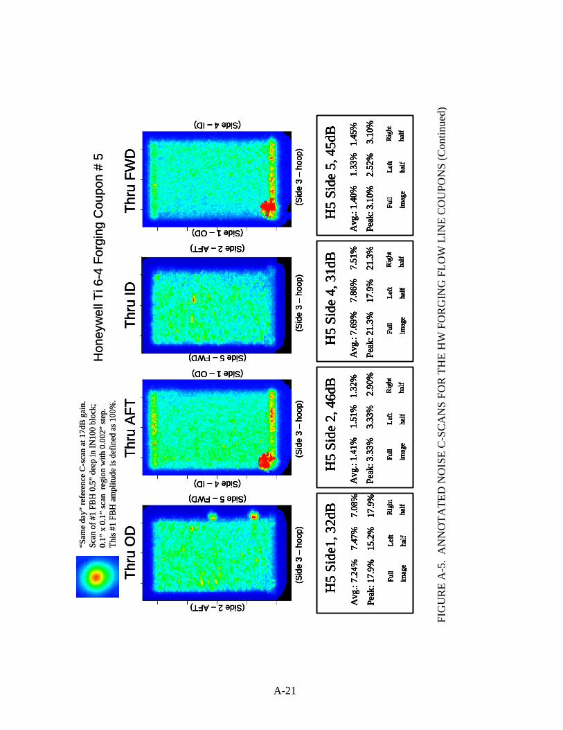
A-21

(Side 2 –AFT)Th

ru O

DTh

ru F

WD

Thru

AFT

Thru

ID

(Sid

e 3

–ho

op)

(Sid

e 3

–ho

op)

(Sid

e 3

–ho

op)

(Sid

e 3

–ho

op)

(Side 2 –AFT)

(Side 5 –FWD)

(Side 5 –FWD)

(Side 4 –ID)

(Side 1 –OD)

(Side 4 –ID)

(Side 1 –OD)

H5

Side

1, 3

2dB

Avg

.: 7.

24%

7

.47%

7

.08%

Peak

: 17.

9%

15.

2%

17.

9%

Full

imag

e

Left

half

Rig

ht

half

H5

Side

2, 4

6dB

Avg

.: 1.

41%

1

.51%

1.

32%

Peak

: 3.3

3%

3.3

3%

2.9

0%

Full

imag

e

Left

half

Rig

ht

half

H5

Side

4, 3

1dB

Avg

.: 7.

69%

7

.86%

7

.51%

Peak

: 21.

3%

17.

9%

21.

3%

Full

imag

e

Left

half

Rig

ht

half

H5

Side

5, 4

5dB

Avg

.: 1.

40%

1

.33%

1.

45%

Peak

: 3.1

0%

2.5

2%

3.1

0%

Full

imag

e

Left

half

Rig

ht

half

Hon

eyw

ell T

i 6-4

For

ging

Cou

pon

# 5

“Sam

e da

y” re

fere

nce

C-s

can

at 1

7dB

gai

n.

Scan

of #

1 FB

H 0

.5”

deep

in IN

100

bloc

k;

0.1”

x 0

.1”

scan

reg

ion

with

0.0

02”

step

. Th

is #

1 FB

H a

mpl

itude

is d

efin

ed a

s 100

%.

(Side 2 –AFT)Th

ru O

DTh

ru F

WD

Thru

AFT

Thru

ID

(Sid

e 3

–ho

op)

(Sid

e 3

–ho

op)

(Sid

e 3

–ho

op)

(Sid

e 3

–ho

op)

(Side 2 –AFT)

(Side 5 –FWD)

(Side 5 –FWD)

(Side 4 –ID)

(Side 1 –OD)

(Side 4 –ID)

(Side 1 –OD)

(Side 2 –AFT)Th

ru O

DTh

ru F

WD

Thru

AFT

Thru

ID

(Sid

e 3

–ho

op)

(Sid

e 3

–ho

op)

(Sid

e 3

–ho

op)

(Sid

e 3

–ho

op)

(Side 2 –AFT)

(Side 5 –FWD)

(Side 5 –FWD)

(Side 4 –ID)

(Side 1 –OD)

(Side 4 –ID)

(Side 1 –OD)

Thru

OD

Thru

FW

DTh

ru A

FTTh

ru ID

(Sid

e 3

–ho

op)

(Sid

e 3

–ho

op)

(Sid

e 3

–ho

op)

(Sid

e 3

–ho

op)

(Side 2 –AFT)

(Side 5 –FWD)

(Side 5 –FWD)

(Side 4 –ID)

(Side 1 –OD)

(Side 4 –ID)

(Side 1 –OD)

H5

Side

1, 3

2dB

Avg

.: 7.

24%

7

.47%

7

.08%

Peak

: 17.

9%

15.

2%

17.

9%

Full

imag

e

Left

half

Rig

ht

half

H5

Side

2, 4

6dB

Avg

.: 1.

41%

1

.51%

1.

32%

Peak

: 3.3

3%

3.3

3%

2.9

0%

Full

imag

e

Left

half

Rig

ht

half

H5

Side

4, 3

1dB

Avg

.: 7.

69%

7

.86%

7

.51%

Peak

: 21.

3%

17.

9%

21.

3%

Full

imag

e

Left

half

Rig

ht

half

H5

Side

5, 4

5dB

Avg

.: 1.

40%

1

.33%

1.

45%

Peak

: 3.1

0%

2.5

2%

3.1

0%

Full

imag

e

Left

half

Rig

ht

half

H5

Side

1, 3

2dB

Avg

.: 7.

24%

7

.47%

7

.08%

Peak

: 17.

9%

15.

2%

17.

9%

Full

imag

e

Left

half

Rig

ht

half

H5

Side

1, 3

2dB

Avg

.: 7.

24%

7

.47%

7

.08%

Peak

: 17.

9%

15.

2%

17.

9%

Full

imag

e

Left

half

Rig

ht

half

H5

Side

1, 3

2dB

Avg

.: 7.

24%

7

.47%

7

.08%

Peak

: 17.

9%

15.

2%

17.

9%

Full

imag

e

Left

half

Rig

ht

half

Avg

.: 7.

24%

7

.47%

7

.08%

Peak

: 17.

9%

15.

2%

17.

9%

Full

imag

e

Left

half

Rig

ht

half

H5

Side

2, 4

6dB

Avg

.: 1.

41%

1

.51%

1.

32%

Peak

: 3.3

3%

3.3

3%

2.9

0%

Full

imag

e

Left

half

Rig

ht

half

H5

Side

2, 4

6dB

Avg

.: 1.

41%

1

.51%

1.

32%

Peak

: 3.3

3%

3.3

3%

2.9

0%

Full

imag

e

Left

half

Rig

ht

half

H5

Side

2, 4

6dB

Avg

.: 1.

41%

1

.51%

1.

32%

Peak

: 3.3

3%

3.3

3%

2.9

0%

Full

imag

e

Left

half

Rig

ht

half

Avg

.: 1.

41%

1

.51%

1.

32%

Peak

: 3.3

3%

3.3

3%

2.9

0%

Full

imag

e

Left

half

Rig

ht

half

H5

Side

4, 3

1dB

Avg

.: 7.

69%

7

.86%

7

.51%

Peak

: 21.

3%

17.

9%

21.

3%

Full

imag

e

Left

half

Rig

ht

half

H5

Side

4, 3

1dB

Avg

.: 7.

69%

7

.86%

7

.51%

Peak

: 21.

3%

17.

9%

21.

3%

Full

imag

e

Left

half

Rig

ht

half

H5

Side

4, 3

1dB

Avg

.: 7.

69%

7

.86%

7

.51%

Peak

: 21.

3%

17.

9%

21.

3%

Full

imag

e

Left

half

Rig

ht

half

Avg

.: 7.

69%

7

.86%

7

.51%

Peak

: 21.

3%

17.

9%

21.

3%

Full

imag

e

Left

half

Rig

ht

half

H5

Side

5, 4

5dB

Avg

.: 1.

40%

1

.33%

1.

45%

Peak

: 3.1

0%

2.5

2%

3.1

0%

Full

imag

e

Left

half

Rig

ht

half

H5

Side

5, 4

5dB

Avg

.: 1.

40%

1

.33%

1.

45%

Peak

: 3.1

0%

2.5

2%

3.1

0%

Full

imag

e

Left

half

Rig

ht

half

H5

Side

5, 4

5dB

Avg

.: 1.

40%

1

.33%

1.

45%

Peak

: 3.1

0%

2.5

2%

3.1

0%

Full

imag

e

Left

half

Rig

ht

half

Avg

.: 1.

40%

1

.33%

1.

45%

Peak

: 3.1

0%

2.5

2%

3.1

0%

Full

imag

e

Left

half

Rig

ht

half

Hon

eyw

ell T

i 6-4

For

ging

Cou

pon

# 5

“Sam

e da

y” re

fere

nce

C-s

can

at 1

7dB

gai

n.

Scan

of #

1 FB

H 0

.5”

deep

in IN

100

bloc

k;

0.1”

x 0

.1”

scan

reg

ion

with

0.0

02”

step

. Th

is #

1 FB

H a

mpl

itude

is d

efin

ed a

s 100

%.

FI

GU

RE

A-5

. A

NN

OTA

TED

NO

ISE

C-S

CA

NS

FOR

TH

E H

W F

OR

GIN

G F

LOW

LIN

E C

OU

PON

S (C

ontin

ued)

A-22

(Side 2 –AFT)

Thru

OD

Thru

FW

DTh

ru A

FTTh

ru ID

(Sid

e 3

–ho

op)

(Sid

e 3

–ho

op)

(Sid

e 3

–ho

op)

(Sid

e 3

–ho

op)

(Side 2 –AFT)

(Side 5 –FWD)

(Side 5 –FWD)

(Side 4 –ID)

(Side 1 –OD)

(Side 4 –ID)

(Side 1 –OD)

H6

Side

1, 3

9dB

Avg

.: 1.

69%

1

.62%

1

.73%

Peak

: 4.1

3%

3.4

5%

4.1

3%

Full

imag

e

Left

half

Rig

ht

half

H6

Side

2, 3

9dB

Avg

.: 1.

78%

1

.76%

1.

80%

Peak

: 3.9

2%

3.2

3%

3.9

2%

Full

imag

e

Left

half

Rig

ht

half

H6

Side

4, 4

4dB

Avg

.: 1.

66%

1

.68%

1.

64%

Peak

: 4.6

5%

4.2

6%

4.6

5%

Full

imag

e

Left

half

Rig

ht

half

H6

Side

5, 4

4dB

Avg

.: 1.

70%

1

.72%

1.

68%

Peak

: 3.8

6%

3.8

6%

3.8

0%

Full

imag

e

Left

half

Rig

ht

half

Hon

eyw

ell T

i 6-4

For

ging

Cou

pon

# 6

“Sam

e da

y” re

fere

nce

C-s

can

at 1

7dB

gai

n.

Scan

of #

1 FB

H 0

.5”

deep

in IN

100

bloc

k;

0.1”

x 0

.1”

scan

reg

ion

with

0.0

02”

step

. Th

is #

1 FB

H a

mpl

itude

is d

efin

ed a

s 100

%.

(Side 2 –AFT)

Thru

OD

Thru

FW

DTh

ru A

FTTh

ru ID

(Sid

e 3

–ho

op)

(Sid

e 3

–ho

op)

(Sid

e 3

–ho

op)

(Sid

e 3

–ho

op)

(Side 2 –AFT)

(Side 5 –FWD)

(Side 5 –FWD)

(Side 4 –ID)

(Side 1 –OD)

(Side 4 –ID)

(Side 1 –OD)

(Side 2 –AFT)

Thru

OD

Thru

FW

DTh

ru A

FTTh

ru ID

(Sid

e 3

–ho

op)

(Sid

e 3

–ho

op)

(Sid

e 3

–ho

op)

(Sid

e 3

–ho

op)

(Side 2 –AFT)

(Side 5 –FWD)

(Side 5 –FWD)

(Side 4 –ID)

(Side 1 –OD)

(Side 4 –ID)

(Side 1 –OD)

Thru

OD

Thru

FW

DTh

ru A

FTTh

ru ID

(Sid

e 3

–ho

op)

(Sid

e 3

–ho

op)

(Sid

e 3

–ho

op)

(Sid

e 3

–ho

op)

(Side 2 –AFT)

(Side 5 –FWD)

(Side 5 –FWD)

(Side 4 –ID)

(Side 1 –OD)

(Side 4 –ID)

(Side 1 –OD)

H6

Side

1, 3

9dB

Avg

.: 1.

69%

1

.62%

1

.73%

Peak

: 4.1

3%

3.4

5%

4.1

3%

Full

imag

e

Left

half

Rig

ht

half

H6

Side

2, 3

9dB

Avg

.: 1.

78%

1

.76%

1.

80%

Peak

: 3.9

2%

3.2

3%

3.9

2%

Full

imag

e

Left

half

Rig

ht

half

H6

Side

4, 4

4dB

Avg

.: 1.

66%

1

.68%

1.

64%

Peak

: 4.6

5%

4.2

6%

4.6

5%

Full

imag

e

Left

half

Rig

ht

half

H6

Side

5, 4

4dB

Avg

.: 1.

70%

1

.72%

1.

68%

Peak

: 3.8

6%

3.8

6%

3.8

0%

Full

imag

e

Left

half

Rig

ht

half

H6

Side

1, 3

9dB

Avg

.: 1.

69%

1

.62%

1

.73%

Peak

: 4.1

3%

3.4

5%

4.1

3%

Full

imag

e

Left

half

Rig

ht

half

H6

Side

1, 3

9dB

Avg

.: 1.

69%

1

.62%

1

.73%

Peak

: 4.1

3%

3.4

5%

4.1

3%

Full

imag

e

Left

half

Rig

ht

half

H6

Side

1, 3

9dB

Avg

.: 1.

69%

1

.62%

1

.73%

Peak

: 4.1

3%

3.4

5%

4.1

3%

Full

imag

e

Left

half

Rig

ht

half

Avg

.: 1.

69%

1

.62%

1

.73%

Peak

: 4.1

3%

3.4

5%

4.1

3%

Full

imag

e

Left

half

Rig

ht

half

H6

Side

2, 3

9dB

Avg

.: 1.

78%

1

.76%

1.

80%

Peak

: 3.9

2%

3.2

3%

3.9

2%

Full

imag

e

Left

half

Rig

ht

half

H6

Side

2, 3

9dB

Avg

.: 1.

78%

1

.76%

1.

80%

Peak

: 3.9

2%

3.2

3%

3.9

2%

Full

imag

e

Left

half

Rig

ht

half

H6

Side

2, 3

9dB

Avg

.: 1.

78%

1

.76%

1.

80%

Peak

: 3.9

2%

3.2

3%

3.9

2%

Full

imag

e

Left

half

Rig

ht

half

Avg

.: 1.

78%

1

.76%

1.

80%

Peak

: 3.9

2%

3.2

3%

3.9

2%

Full

imag

e

Left

half

Rig

ht

half

H6

Side

4, 4

4dB

Avg

.: 1.

66%

1

.68%

1.

64%

Peak

: 4.6

5%

4.2

6%

4.6

5%

Full

imag

e

Left

half

Rig

ht

half

H6

Side

4, 4

4dB

Avg

.: 1.

66%

1

.68%

1.

64%

Peak

: 4.6

5%

4.2

6%

4.6

5%

Full

imag

e

Left

half

Rig

ht

half

H6

Side

4, 4

4dB

Avg

.: 1.

66%

1

.68%

1.

64%

Peak

: 4.6

5%

4.2

6%

4.6

5%

Full

imag

e

Left

half

Rig

ht

half

Avg

.: 1.

66%

1

.68%

1.

64%

Peak

: 4.6

5%

4.2

6%

4.6

5%

Full

imag

e

Left

half

Rig

ht

half

H6

Side

5, 4

4dB

Avg

.: 1.

70%

1

.72%

1.

68%

Peak

: 3.8

6%

3.8

6%

3.8

0%

Full

imag

e

Left

half

Rig

ht

half

H6

Side

5, 4

4dB

Avg

.: 1.

70%

1

.72%

1.

68%

Peak

: 3.8

6%

3.8

6%

3.8

0%

Full

imag

e

Left

half

Rig

ht

half

H6

Side

5, 4

4dB

Avg

.: 1.

70%

1

.72%

1.

68%

Peak

: 3.8

6%

3.8

6%

3.8

0%

Full

imag

e

Left

half

Rig

ht

half

Avg

.: 1.

70%

1

.72%

1.

68%

Peak

: 3.8

6%

3.8

6%

3.8

0%

Full

imag

e

Left

half

Rig

ht

half

Hon

eyw

ell T

i 6-4

For

ging

Cou

pon

# 6

“Sam

e da

y” re

fere

nce

C-s

can

at 1

7dB

gai

n.

Scan

of #

1 FB

H 0

.5”

deep

in IN

100

bloc

k;

0.1”

x 0

.1”

scan

reg

ion

with

0.0

02”

step

. Th

is #

1 FB

H a

mpl

itude

is d

efin

ed a

s 100

%.

FIG

UR

E A

-5.

AN

NO

TATE

D N

OIS

E C

-SC

AN

S FO

R T

HE

HW

FO

RG

ING

FLO

W L

INE

CO

UPO

NS

(Con

tinue

d)

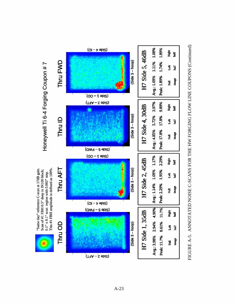
A-23

FI

GU

RE

A-5

. A

NN

OTA

TED

NO

ISE

C-S

CA

NS

FOR

TH

E H

W F

OR

GIN

G F

LOW

LIN

E C

OU

PON

S (C

ontin

ued)

(Side 2 –AFT)

Thru

OD

Thru

FW

DTh

ru A

FTTh

ru ID

(Sid

e 3

–ho

op)

(Sid

e 3

–ho

op)

(Sid

e 3

–ho

op)

(Sid

e 3

–ho

op)

(Side 2 –AFT)

(Side 5 –FWD)

(Side 5 –FWD)

(Side 4 –ID)

(Side 1 –OD)

(Side 4 –ID)

(Side 1 –OD)

H7

Side

1, 3

5dB

Avg

.: 3.

98%

2

.94%

4

.90%

Peak

: 11.

7%

8.6

1%

11.

7%

Full

imag

e

Left

half

Rig

ht

half

H7

Side

2, 4

5dB

Avg

.: 1.

14%

1

.09%

1

.17%

Peak

: 2.2

9%

1.9

5%

2.2

9%

Full

imag

e

Left

half

Rig

ht

half

H7

Side

4, 3

0dB

Avg

.: 4.

85%

5

.72%

3

.97%

Peak

: 17.

8%

17.

8%

9.8

9%

Full

imag

e

Left

half

Rig

ht

half

H7

Side

5, 4

6dB

Avg

.: 1.

09%

1

.11%

1

.08%

Peak

: 1.8

9%

1.7

4%

1.8

9%

Full

imag

e

Left

half

Rig

ht

half

Hon

eyw

ell T

i 6-4

For

ging

Cou

pon

# 7

“Sam

e da

y” re

fere

nce

C-s

can

at 1

7dB

gai

n.

Scan

of #

1 FB

H 0

.5”

deep

in IN

100

bloc

k;

0.1”

x 0

.1”

scan

reg

ion

with

0.0

02”

step

. Th

is #

1 FB

H a

mpl

itude

is d

efin

ed a

s 100

%.

(Side 2 –AFT)

Thru

OD

Thru

FW

DTh

ru A

FTTh

ru ID

(Sid

e 3

–ho

op)

(Sid

e 3

–ho

op)

(Sid

e 3

–ho

op)

(Sid

e 3

–ho

op)

(Side 2 –AFT)

(Side 5 –FWD)

(Side 5 –FWD)

(Side 4 –ID)

(Side 1 –OD)

(Side 4 –ID)

(Side 1 –OD)

(Side 2 –AFT)

Thru

OD

Thru

FW

DTh

ru A

FTTh

ru ID

(Sid

e 3

–ho

op)

(Sid

e 3

–ho

op)

(Sid

e 3

–ho

op)

(Sid

e 3

–ho

op)

(Side 2 –AFT)

(Side 5 –FWD)

(Side 5 –FWD)

(Side 4 –ID)

(Side 1 –OD)

(Side 4 –ID)

(Side 1 –OD)

Thru

OD

Thru

FW

DTh

ru A

FTTh

ru ID

(Sid

e 3

–ho

op)

(Sid

e 3

–ho

op)

(Sid

e 3

–ho

op)

(Sid

e 3

–ho

op)

(Side 2 –AFT)

(Side 5 –FWD)

(Side 5 –FWD)

(Side 4 –ID)

(Side 1 –OD)

(Side 4 –ID)

(Side 1 –OD)

H7

Side

1, 3

5dB

Avg

.: 3.

98%

2

.94%

4

.90%

Peak

: 11.

7%

8.6

1%

11.

7%

Full

imag

e

Left

half

Rig

ht

half

H7

Side

2, 4

5dB

Avg

.: 1.

14%

1

.09%

1

.17%

Peak

: 2.2

9%

1.9

5%

2.2

9%

Full

imag

e

Left

half

Rig

ht

half

H7

Side

4, 3

0dB

Avg

.: 4.

85%

5

.72%

3

.97%

Peak

: 17.

8%

17.

8%

9.8

9%

Full

imag

e

Left

half

Rig

ht

half

H7

Side

5, 4

6dB

Avg

.: 1.

09%

1

.11%

1

.08%

Peak

: 1.8

9%

1.7

4%

1.8

9%

Full

imag

e

Left

half

Rig

ht

half

H7

Side

1, 3

5dB

Avg

.: 3.

98%

2

.94%

4

.90%

Peak

: 11.

7%

8.6

1%

11.

7%

Full

imag

e

Left

half

Rig

ht

half

H7

Side

1, 3

5dB

Avg

.: 3.

98%

2

.94%

4

.90%

Peak

: 11.

7%

8.6

1%

11.

7%

Full

imag

e

Left

half

Rig

ht

half

H7

Side

1, 3

5dB

Avg

.: 3.

98%

2

.94%

4

.90%

Peak

: 11.

7%

8.6

1%

11.

7%

Full

imag

e

Left

half

Rig

ht

half

Avg

.: 3.

98%

2

.94%

4

.90%

Peak

: 11.

7%

8.6

1%

11.

7%

Full

imag

e

Left

half

Rig

ht

half

H7

Side

2, 4

5dB

Avg

.: 1.

14%

1

.09%

1

.17%

Peak

: 2.2

9%

1.9

5%

2.2

9%

Full

imag

e

Left

half

Rig

ht

half

H7

Side

2, 4

5dB

Avg

.: 1.

14%

1

.09%

1

.17%

Peak

: 2.2

9%

1.9

5%

2.2

9%

Full

imag

e

Left

half

Rig

ht

half

H7

Side

2, 4

5dB

Avg

.: 1.

14%

1

.09%

1

.17%

Peak

: 2.2

9%

1.9

5%

2.2

9%

Full

imag

e

Left

half

Rig

ht

half

Avg

.: 1.

14%

1

.09%

1

.17%

Peak

: 2.2

9%

1.9

5%

2.2

9%

Full

imag

e

Left

half

Rig

ht

half

H7

Side

4, 3

0dB

Avg

.: 4.

85%

5

.72%

3

.97%

Peak

: 17.

8%

17.

8%

9.8

9%

Full

imag

e

Left

half

Rig

ht

half

H7

Side

4, 3

0dB

Avg

.: 4.

85%

5

.72%

3

.97%

Peak

: 17.

8%

17.

8%

9.8

9%

Full

imag

e

Left

half

Rig

ht

half

H7

Side

4, 3

0dB

Avg

.: 4.

85%

5

.72%

3

.97%

Peak

: 17.

8%

17.

8%

9.8

9%

Full

imag

e

Left

half

Rig

ht

half

Avg

.: 4.

85%

5

.72%

3

.97%

Peak

: 17.

8%

17.

8%

9.8

9%

Full

imag

e

Left

half

Rig

ht

half

H7

Side

5, 4

6dB

Avg

.: 1.

09%

1

.11%

1

.08%

Peak

: 1.8

9%

1.7

4%

1.8

9%

Full

imag

e

Left

half

Rig

ht

half

H7

Side

5, 4

6dB

Avg

.: 1.

09%

1

.11%

1

.08%

Peak

: 1.8

9%

1.7

4%

1.8

9%

Full

imag

e

Left

half

Rig

ht

half

H7

Side

5, 4

6dB

Avg

.: 1.

09%

1

.11%

1

.08%

Peak

: 1.8

9%

1.7

4%

1.8

9%

Full

imag

e

Left

half

Rig

ht

half

Avg

.: 1.

09%

1

.11%

1

.08%

Peak

: 1.8

9%

1.7

4%

1.8

9%

Full

imag

e

Left

half

Rig

ht

half

Hon

eyw

ell T

i 6-4

For

ging

Cou

pon

# 7

“Sam

e da

y” re

fere

nce

C-s

can

at 1

7dB

gai

n.

Scan

of #

1 FB

H 0

.5”

deep

in IN

100

bloc

k;

0.1”

x 0

.1”

scan

reg

ion

with

0.0

02”

step

. Th

is #

1 FB

H a

mpl

itude

is d

efin

ed a

s 100

%.

A-24

FI

GU

RE

A-5

. A

NN

OTA

TED

NO

ISE

C-S

CA

NS

FOR

TH

E H

W F

OR

GIN

G F

LOW

LIN

E C

OU

PON

S (C

ontin

ued)

(Side 2 –AFT)

Thru

OD

Thru

FW

DTh

ru A

FTTh

ru ID

(Sid

e 3

–ho

op)

(Sid

e 3

–ho

op)

(Sid

e 3

–ho

op)

(Sid

e 3

–ho

op)

(Side 2 –AFT)

(Side 5 –FWD)

(Side 5 –FWD)

(Side 4 –ID)

(Side 1 –OD)

(Side 4 –ID)

(Side 1 –OD)

H8

Side

1, 4

5dB

Avg

.: 1.

22%

1

.33%

1

.11%

Peak

: 3.1

7%

3.1

7%

2.1

6%

Full

imag

e

Left

half

Rig

ht

half

H8

Side

2, 4

2dB

Avg

.: 1.

59%

1

.64%

1

.51%

Peak

: 4.3

2%

4.3

2%

2.8

4%

Full

imag

e

Left

half

Rig

ht

half

H8

Side

4, 4

3dB

Avg

.: 1.

36%

1

.35%

1

.37%

Peak

: 3.5

7%

3.5

7%

2.7

1%

Full

imag

e

Left

half

Rig

ht

half

H8

Side

5, 4

5dB

Avg

.: 1.

31%

1

.36%

1

.25%

Peak

: 3.1

7%

3.1

7%

2.1

6%

Full

imag

e

Left

half

Rig

ht

half

Hon

eyw

ell T

i 6-4

For

ging

Cou

pon

# 8

“Sam

e da

y” re

fere

nce

C-s

can

at 1

7dB

gai

n.

Scan

of #

1 FB

H 0

.5”

deep

in IN

100

bloc

k;

0.1”

x 0

.1”

scan

reg

ion

with

0.0

02”

step

. Th

is #

1 FB

H a

mpl

itude

is d

efin

ed a

s 100

%.

(Side 2 –AFT)

Thru

OD

Thru

FW

DTh

ru A

FTTh

ru ID

(Sid

e 3

–ho

op)

(Sid

e 3

–ho

op)

(Sid

e 3

–ho

op)

(Sid

e 3

–ho

op)

(Side 2 –AFT)

(Side 5 –FWD)

(Side 5 –FWD)

(Side 4 –ID)

(Side 1 –OD)

(Side 4 –ID)

(Side 1 –OD)

(Side 2 –AFT)

Thru

OD

Thru

FW

DTh

ru A

FTTh

ru ID

(Sid

e 3

–ho

op)

(Sid

e 3

–ho

op)

(Sid

e 3

–ho

op)

(Sid

e 3

–ho

op)

(Side 2 –AFT)

(Side 5 –FWD)

(Side 5 –FWD)

(Side 4 –ID)

(Side 1 –OD)

(Side 4 –ID)

(Side 1 –OD)

Thru

OD

Thru

FW

DTh

ru A

FTTh

ru ID

(Sid

e 3

–ho

op)

(Sid

e 3

–ho

op)

(Sid

e 3

–ho

op)

(Sid

e 3

–ho

op)

(Side 2 –AFT)

(Side 5 –FWD)

(Side 5 –FWD)

(Side 4 –ID)

(Side 1 –OD)

(Side 4 –ID)

(Side 1 –OD)

H8

Side

1, 4

5dB

Avg

.: 1.

22%

1

.33%

1

.11%

Peak

: 3.1

7%

3.1

7%

2.1

6%

Full

imag

e

Left

half

Rig

ht

half

H8

Side

2, 4

2dB

Avg

.: 1.

59%

1

.64%

1

.51%

Peak

: 4.3

2%

4.3

2%

2.8

4%

Full

imag

e

Left

half

Rig

ht

half

H8

Side

4, 4

3dB

Avg

.: 1.

36%

1

.35%

1

.37%

Peak

: 3.5

7%

3.5

7%

2.7

1%

Full

imag

e

Left

half

Rig

ht

half

H8

Side

5, 4

5dB

Avg

.: 1.

31%

1

.36%

1

.25%

Peak

: 3.1

7%

3.1

7%

2.1

6%

Full

imag

e

Left

half

Rig

ht

half

H8

Side

1, 4

5dB

Avg

.: 1.

22%

1

.33%

1

.11%

Peak

: 3.1

7%

3.1

7%

2.1

6%

Full

imag

e

Left

half

Rig

ht

half

H8

Side

1, 4

5dB

Avg

.: 1.

22%

1

.33%

1

.11%

Peak

: 3.1

7%

3.1

7%

2.1

6%

Full

imag

e

Left

half

Rig

ht

half

H8

Side

1, 4

5dB

Avg

.: 1.

22%

1

.33%

1

.11%

Peak

: 3.1

7%

3.1

7%

2.1

6%

Full

imag

e

Left

half

Rig

ht

half

Avg

.: 1.

22%

1

.33%

1

.11%

Peak

: 3.1

7%

3.1

7%

2.1

6%

Full

imag

e

Left

half

Rig

ht

half

H8

Side

2, 4

2dB

Avg

.: 1.

59%

1

.64%

1

.51%

Peak

: 4.3

2%

4.3

2%

2.8

4%

Full

imag

e

Left

half

Rig

ht

half

H8

Side

2, 4

2dB

Avg

.: 1.

59%

1

.64%

1

.51%

Peak

: 4.3

2%

4.3

2%

2.8

4%

Full

imag

e

Left

half

Rig

ht

half

H8

Side

2, 4

2dB

Avg

.: 1.

59%

1

.64%

1

.51%

Peak

: 4.3

2%

4.3

2%

2.8

4%

Full

imag

e

Left

half

Rig

ht

half

Avg

.: 1.

59%

1

.64%

1

.51%

Peak

: 4.3

2%

4.3

2%

2.8

4%

Full

imag

e

Left

half

Rig

ht

half

H8

Side

4, 4

3dB

Avg

.: 1.

36%

1

.35%

1

.37%

Peak

: 3.5

7%

3.5

7%

2.7

1%

Full

imag

e

Left

half

Rig

ht

half

H8

Side

4, 4

3dB

Avg

.: 1.

36%

1

.35%

1

.37%

Peak

: 3.5

7%

3.5

7%

2.7

1%

Full

imag

e

Left

half

Rig

ht

half

H8

Side

4, 4

3dB

Avg

.: 1.

36%

1

.35%

1

.37%

Peak

: 3.5

7%

3.5

7%

2.7

1%

Full

imag

e

Left

half

Rig

ht

half

Avg

.: 1.

36%

1

.35%

1

.37%

Peak

: 3.5

7%

3.5

7%

2.7

1%

Full

imag

e

Left

half

Rig

ht

half

H8

Side

5, 4

5dB

Avg

.: 1.

31%

1

.36%

1

.25%

Peak

: 3.1

7%

3.1

7%

2.1

6%

Full

imag

e

Left

half

Rig

ht

half

H8

Side

5, 4

5dB

Avg

.: 1.

31%

1

.36%

1

.25%

Peak

: 3.1

7%

3.1

7%

2.1

6%

Full

imag

e

Left

half

Rig

ht

half

H8

Side

5, 4

5dB

Avg

.: 1.

31%

1

.36%

1

.25%

Peak

: 3.1

7%

3.1

7%

2.1

6%

Full

imag

e

Left

half

Rig

ht

half

Avg

.: 1.

31%

1

.36%

1

.25%

Peak

: 3.1

7%

3.1

7%

2.1

6%

Full

imag

e

Left

half

Rig

ht

half

Hon

eyw

ell T

i 6-4

For

ging

Cou

pon

# 8

“Sam

e da

y” re

fere

nce

C-s

can

at 1

7dB

gai

n.

Scan

of #

1 FB

H 0

.5”

deep

in IN

100

bloc

k;

0.1”

x 0

.1”

scan

reg

ion

with

0.0

02”

step

. Th

is #

1 FB

H a

mpl

itude

is d

efin

ed a

s 100

%.

A-25

FI

GU

RE

A-6

. LO

NG

ITU

DIN

AL-

WA

VE

ATT

ENU

ATI

ON

-VER

SUS-

FREQ

UEN

CY

CU

RV

ES F

OR

TH

E

FOR

GIN

G F

LOW

LIN

E C

OU

PON

S IN

Nep

ers/

cm U

NIT

S, A

S M

EASU

RED

AT

ISU

PW#1

Sid

e1&

2 A

ttenu

atio

n

0.00

0.03

0.06

0.09

0.12

0.15

02

46

810

1214

1618

20

Freq

uenc

y (M

Hz)

Att (Np/cm)

Att_

Sid

e 1

Att_

Sid

e2

PW#2

Sid

e1&

2 A

tten

uatio

n

0.00

0.03

0.06

0.09

0.12

0.15

02

46

810

1214

1618

20

Freq

uenc

y (M

Hz)

Att (Np/cm)

Att_

Sid

e 1

Att_

Sid

e2

PW#4

Sid

e1&

2 A

tten

uatio

n

0.00

0.03

0.06

0.09

0.12

0.15

02

46

810

1214

1618

20

Freq

uenc

y (M

Hz)

Att (Np/cm)

Att_

Sid

e 1

Att_

Sid

e2

PW#5

Sid

e1&

2 A

ttenu

atio

n

0.00

0.05

0.10

0.15

0.20

0.25

02

46

810

1214

1618

20

Freq

uenc

y (M

Hz)

Att (Np/cm)

Att_

Sid

e 1

Att_

Sid

e2

PW#1

Sid

e1&

2 A

ttenu

atio

n

0.00

0.03

0.06

0.09

0.12

0.15

02

46

810

1214

1618

20

Freq

uenc

y (M

Hz)

Att (Np/cm)

Att_

Sid

e 1

Att_

Sid

e2

PW#2

Sid

e1&

2 A

tten

uatio

n

0.00

0.03

0.06

0.09

0.12

0.15

02

46

810

1214

1618

20

Freq

uenc

y (M

Hz)

Att (Np/cm)

Att_

Sid

e 1

Att_

Sid

e2

PW#4

Sid

e1&

2 A

tten

uatio

n

0.00

0.03

0.06

0.09

0.12

0.15

02

46

810

1214

1618

20

Freq

uenc

y (M

Hz)

Att (Np/cm)

Att_

Sid

e 1

Att_

Sid

e2

PW#5

Sid

e1&

2 A

ttenu

atio

n

0.00

0.05

0.10

0.15

0.20

0.25

02

46

810

1214

1618

20

Freq

uenc

y (M

Hz)

Att (Np/cm)

Att_

Sid

e 1

Att_

Sid

e2

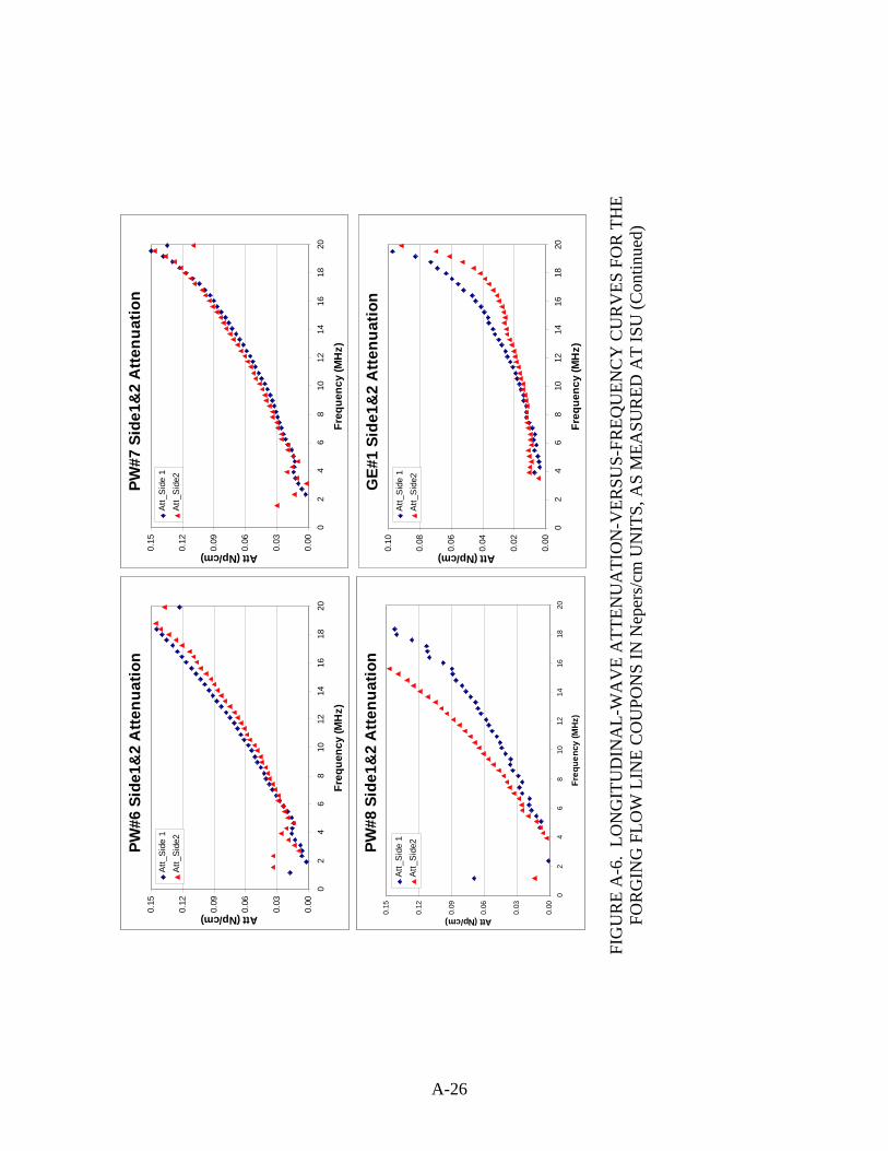
A-26

FI

GU

RE

A-6

. LO

NG

ITU

DIN

AL-

WA

VE

ATT

ENU

ATI

ON

-VER

SUS-

FREQ

UEN

CY

CU

RV

ES F

OR

TH

E

FOR

GIN

G F

LOW

LIN

E C

OU

PON

S IN

Nep

ers/

cm U

NIT

S, A

S M

EASU

RED

AT

ISU

(Con

tinue

d)

PW#6

Sid

e1&

2 A

ttenu

atio

n

0.00

0.03

0.06

0.09

0.12

0.15

02

46

810

1214

1618

20

Freq

uenc

y (M

Hz)

Att (Np/cm)

Att_

Sid

e 1

Att_

Sid

e2

PW#7

Sid

e1&

2 A

ttenu

atio

n

0.00

0.03

0.06

0.09

0.12

0.15

02

46

810

1214

1618

20

Freq

uenc

y (M

Hz)

Att (Np/cm)

Att_

Sid

e 1

Att_

Sid

e2

PW#8

Sid

e1&

2 A

ttenu

atio

n

0.00

0.03

0.06

0.09

0.12

0.15

02

46

810

1214

1618

20

Freq

uenc

y (M

Hz)

Att (Np/cm)

Att_

Sid

e 1

Att_

Sid

e2

GE#

1 Si

de1&

2 A

tten

uatio

n

0.00

0.02

0.04

0.06

0.08

0.10

02

46

810

1214

1618

20

Freq

uenc

y (M

Hz)

Att (Np/cm)

Att_

Sid

e 1

Att_

Sid

e2

PW#6

Sid

e1&

2 A

ttenu

atio

n

0.00

0.03

0.06

0.09

0.12

0.15

02

46

810

1214

1618

20

Freq

uenc

y (M

Hz)

Att (Np/cm)

Att_

Sid

e 1

Att_

Sid

e2

PW#7

Sid

e1&

2 A

ttenu

atio

n

0.00

0.03

0.06

0.09

0.12

0.15

02

46

810

1214

1618

20

Freq

uenc

y (M

Hz)

Att (Np/cm)

Att_

Sid

e 1

Att_

Sid

e2

PW#8

Sid

e1&

2 A

ttenu

atio

n

0.00

0.03

0.06

0.09

0.12

0.15

02

46

810

1214

1618

20

Freq

uenc

y (M

Hz)

Att (Np/cm)

Att_

Sid

e 1

Att_

Sid

e2

GE#

1 Si

de1&

2 A

tten

uatio

n

0.00

0.02

0.04

0.06

0.08

0.10

02

46

810

1214

1618

20

Freq

uenc

y (M

Hz)

Att (Np/cm)

Att_

Sid

e 1

Att_

Sid

e2

A-27

FI

GU

RE

A-6

. LO

NG

ITU

DIN

AL-

WA

VE

ATT

ENU

ATI

ON

-VER

SUS-

FREQ

UEN

CY

CU

RV

ES F

OR

TH

E

FOR

GIN

G F

LOW

LIN

E C

OU

PON

S IN

Nep

ers/

cm U

NIT

S, A

S M

EASU

RED

AT

ISU

(Con

tinue

d)

GE#

4 Si

de1&

2 A

ttenu

atio

n

0.00

0.03

0.06

0.09

0.12

0.15

02

46

810

1214

1618

20

Freq

uenc

y (M

Hz)

Att (Np/cm)

Att_

Sid

e 1

Att_

Sid

e2

GE#

5 Si

de1&

2 A

tten

uatio

n

0.00

0.03

0.06

0.09

0.12

02

46

810

1214

1618

20

Freq

uenc

y (M

Hz)

Att (Np/cm)

Att_

Sid

e 1

Att_

Sid

e2

GE#

6 Si

de1&

2 A

tten

uatio

n

0.00

0.03

0.06

0.09

0.12

02

46

810

1214

1618

20

Freq

uenc

y (M

Hz)

Att (Np/cm)

Att_

Sid

e 1

Att_

Sid

e2

GE#

7 Si

de1&

2 A

tten

uatio

n

0.00

0.03

0.06

0.09

0.12

02

46

810

1214

1618

20

Freq

uenc

y (M

Hz)

Att (Np/cm)

Att_

Sid

e 1

Att_

Sid

e2

GE#

4 Si

de1&

2 A

ttenu

atio

n

0.00

0.03

0.06

0.09

0.12

0.15

02

46

810

1214

1618

20

Freq

uenc

y (M

Hz)

Att (Np/cm)

Att_

Sid

e 1

Att_

Sid

e2

GE#

5 Si

de1&

2 A

tten

uatio

n

0.00

0.03

0.06

0.09

0.12

02

46

810

1214

1618

20

Freq

uenc

y (M

Hz)

Att (Np/cm)

Att_

Sid

e 1

Att_

Sid

e2

GE#

6 Si

de1&

2 A

tten

uatio

n

0.00

0.03

0.06

0.09

0.12

02

46

810

1214

1618

20

Freq

uenc

y (M

Hz)

Att (Np/cm)

Att_

Sid

e 1

Att_

Sid

e2

GE#

7 Si

de1&

2 A

tten

uatio

n

0.00

0.03

0.06

0.09

0.12

02

46

810

1214

1618

20

Freq

uenc

y (M

Hz)

Att (Np/cm)

Att_

Sid

e 1

Att_

Sid

e2

A-28

FI

GU

RE

A-6

. LO

NG

ITU

DIN

AL-

WA

VE

ATT

ENU

ATI

ON

-VER

SUS-

FREQ

UEN

CY

CU

RV

ES F

OR

TH

E

FOR

GIN

G F

LOW

LIN

E C

OU

PON

S IN

Nep

ers/

cm U

NIT

S, A

S M

EASU

RED

AT

ISU

(Con

tinue

d)

Hon

eyw

ell#

1 Si

de1&

2 A

ttenu

atio

n

0.00

0.03

0.06

0.09

0.12

0.15

02

46

810

1214

1618

20

Freq

uenc

y (M

Hz)

Att (Np/cm)

Att_

Sid

e 1

Att_

Sid

e2

Hon

eyw

ell#

2 Si

de1&

2 A

ttenu

atio

n

0.00

0.03

0.06

0.09

0.12

0.15

02

46

810

1214

1618

20

Freq

uenc

y (M

Hz)

Att (Np/cm)

Att_

Sid

e 1

Att_

Sid

e2

Hon

eyw

ell#

3 Si

de1&

2 A

ttenu

atio

n

0.00

0.03

0.06

0.09

0.12

02

46

810

1214

1618

20

Freq

uenc

y (M

Hz)

Att (Np/cm)

Att_

Sid

e 1

Att_

Sid

e2

Hon

eyw

ell#

4 Si

de1&

2 A

ttenu

atio

n

0.00

0.03

0.06

0.09

0.12

02

46

810

1214

1618

20

Freq

uenc

y (M

Hz)

Att (Np/cm)

Att_

Sid

e 1

Att_

Sid

e2

Hon

eyw

ell#

1 Si

de1&

2 A

ttenu

atio

n

0.00

0.03

0.06

0.09

0.12

0.15

02

46

810

1214

1618

20

Freq

uenc

y (M

Hz)

Att (Np/cm)

Att_

Sid

e 1

Att_

Sid

e2

Hon

eyw

ell#

2 Si

de1&

2 A

ttenu

atio

n

0.00

0.03

0.06

0.09

0.12

0.15

02

46

810

1214

1618

20

Freq

uenc

y (M

Hz)

Att (Np/cm)

Att_

Sid

e 1

Att_

Sid

e2

Hon

eyw

ell#

3 Si

de1&

2 A

ttenu

atio

n

0.00

0.03

0.06

0.09

0.12

02

46

810

1214

1618

20

Freq

uenc

y (M

Hz)

Att (Np/cm)

Att_

Sid

e 1

Att_

Sid

e2

Hon

eyw

ell#

4 Si

de1&

2 A

ttenu

atio

n

0.00

0.03

0.06

0.09

0.12

02

46

810

1214

1618

20

Freq

uenc

y (M

Hz)

Att (Np/cm)

Att_

Sid

e 1

Att_

Sid

e2

A-29

FI

GU

RE

A-6

. LO

NG

ITU

DIN

AL-

WA

VE

ATT

ENU

ATI

ON

-VER

SUS-

FREQ

UEN

CY

CU

RV

ES F

OR

TH

E

FOR

GIN

G F

LOW

LIN

E C

OU

PON

S IN

Nep

ers/

cm U

NIT

S, A

S M

EASU

RED

AT

ISU

(Con

tinue

d)

Hon

eyw

ell#

6 Si

de1&

2 A

tten

uatio

n

0.00

0.03

0.06

0.09

0.12

02

46

810

1214

1618

20

Freq

uenc

y (M

Hz)

Att (Np/cm)

Att_

Sid

e 1

Att_

Sid

e2

Hon

eyw

ell#

7 Si

de1&

2 A

tten

uatio

n

0.00

0.05

0.10

0.15

0.20

0.25

0.30

02

46

810

1214

1618

20

Freq

uenc

y (M

Hz)

Att (Np/cm)

Att_

Sid

e 1

Att_

Sid

e2

Hon

eyw

ell#

8 Si

de1&

2 A

tten

uatio

n

0.00

0.03

0.06

0.09

0.12

0.15

0.18

02

46

810

1214

1618

20

Freq

uenc

y (M

Hz)

Att (Np/cm)

Att_

Sid

e 1

Att_

Sid

e2

Hon

eyw

ell#

5 Si

de1&

2 A

ttenu

atio

n

0.00

0.05

0.10

0.15

0.20

0.25

02

46

810

1214

1618

20

Freq

uenc

y (M

Hz)

Att (Np/cm)

Att_

Sid

e 1

Att_

Sid

e 2

Hon

eyw

ell#

6 Si

de1&

2 A

tten

uatio

n

0.00

0.03

0.06

0.09

0.12

02

46

810

1214

1618

20

Freq

uenc

y (M

Hz)

Att (Np/cm)

Att_

Sid

e 1

Att_

Sid

e2

Hon

eyw

ell#

7 Si

de1&

2 A

tten

uatio

n

0.00

0.05

0.10

0.15

0.20

0.25

0.30

02

46

810

1214

1618

20

Freq

uenc

y (M

Hz)

Att (Np/cm)

Att_

Sid

e 1

Att_

Sid

e2

Hon

eyw

ell#

8 Si

de1&

2 A

tten

uatio

n

0.00

0.03

0.06

0.09

0.12

0.15

0.18

02

46

810

1214

1618

20

Freq

uenc

y (M

Hz)

Att (Np/cm)

Att_

Sid

e 1

Att_

Sid

e2

Hon

eyw

ell#

5 Si

de1&

2 A

ttenu

atio

n

0.00

0.05

0.10

0.15

0.20

0.25

02

46

810

1214

1618

20

Freq

uenc

y (M

Hz)

Att (Np/cm)

Att_

Sid

e 1

Att_

Sid

e 2

A-30

TAB

LE A

-1.

GR

AIN

NO

ISE

STA

TIST

ICS

FOR

TH

E FO

RG

ING

FLO

W L

INE

CO

UPO

NS,

EX

TRA

CTE

D F

RO

M

FIG

UR

ES A

-4 A

ND

A-6

(The

last

four

col

umns

are

of c

hief

inte

rest

and

dis

play

the

aver

age,

stan

dard

dev

iatio

n, m

inim

um, a

nd m

axim

um n

oise

am

plitu

des

usin

g a

scal

e in

whi

ch 1

00 e

qual

s the

pea

k am

plitu

de fr

om a

Ti-6

-4 #

1 fla

t-bot

tom

hol

e (F

BH

) in

the

foca

l zon

e.)

Ta

bula

r For

m o

f the

Noi

se D

ata

for G

E F

orgi

ng C

oupo

ns

S

umm

ary

of G

rain

Noi

se M

easu

rem

ents

on

G

E T

i-6-4

For

ging

s S

peci

men

s R

aw d

ata

valu

es o

n a

scal

e of

0-2

54

Nor

mal

ized

by

0.5″

dee

p #1

FB

H in

IN

100

= 10

0 (M

easu

red

FBH

had

pe

ak re

spon

se o

f 216

at 1

5 dB

)

Nor

mal

ized

by

#1 F

BH

in

foca

l zon

e in

Ti-6

-4 =

100

(E

stim

ated

usi

ng IS

U m

odel

s)

Inde

x IS

U N

ame

dB

Set

ting

Ave

. Noi

se

Sig

ma

Min

. M

ax.

Ave

. S

igm

a M

in.

Max

. A

ve.

Sig

ma

Min

. M

ax.

1 G

E1_

S1_

L 52

13

2.09

21

.31

84

244

0.86

0.14

0.

551.

60

0.28

0.

04

0.18

0.51

2 G

E1_

S1_

R

52

149.

64

20.7

510

0 24

4 0.

980.

14

0.65

1.60

0.

32

0.04

0.

210.

513

GE

1_S

4_L

52

155.

16

20.1

498

24

4 1.

020.

13

0.64

1.60

0.

33

0.04

0.

210.

514

GE

1_S

4_R

52

13

7.92

19

.73

86

227

0.90

0.13

0.

561.

48

0.29

0.

04

0.18

0.48

5 G

E1_

S2_

L 37

11

9.37

33

.27

64

306

4.39

1.22

2.

3511

.25

1.42

0.

39

0.76

3.63

6 G

E1_

S2_

R

37

102.

46

34.6

036

24

1 3.

771.

27

1.32

8.86

1.

22

0.41

0.

432.

867

GE

1_S

5_L

41

148.

79

25.3

184

31

5 3.

450.

59

1.95

7.31

1.

11

0.19

0.

632.

368

GE

1_S

5_R

41

14

5.53

23

.15

84

244

3.38

0.54

1.

955.

66

1.09

0.

17

0.63

1.83

1

GE

4_S

1_L

34

111.

59

35.1

742

25

2 5.

801.

83

2.18

13.0

9 1.

87

0.59

0.

704.

222

GE

4_S

1_R

34

10

2.45

33

.40

42

288

5.32

1.73

2.

1814

.96

1.72

0.

56

0.70

4.83

3 G

E4_

S4_

L 34

76

.91

18.1

844

17

0 4.

000.

94

2.29

8.83

1.

29

0.30

0.

742.

854

GE

4_S

4_R

34

60

.66

16.2

830

15

8 3.

150.

85

1.56

8.21

1.

02

0.27

0.

502.

655

GE

4_S

2_L

45

140.

52

32.9

372

37

7 2.

060.

48

1.05

5.52

0.

66

0.16

0.

341.

786

GE

4_S

2_R

45

93

.01

20.9

054

32

0 1.

360.

31

0.79

4.68

0.

44

0.10

0.

261.

517

GE

4_S

5_L

45

87.5

7 14

.13

58

160

1.28

0.21

0.

852.

34

0.41

0.

07

0.27

0.76

8 G

E4_

S5_

R

45

100.

23

21.1

360

24

1 1.

470.

31

0.88

3.53

0.

47

0.10

0.

281.

14

1 G

E5_

S1_

L 36

12

7.35

34

.15

52

291

5.25

1.41

2.

1512

.01

1.70

0.

45

0.69

3.87

2 G

E5_

S1_

R

36

31.8

0 10

.70

18

118

1.31

0.44

0.

744.

87

0.42

0.

14

0.24

1.57

3 G

E5_

S4_

L 36

31

.17

7.34

20

90

1.29

0.30

0.

833.

71

0.41

0.

10

0.27

1.20

4 G

E5_

S4_

R

36

118.

21

29.9

960

27

5 4.

881.

24

2.48

11.3

5 1.

57

0.40

0.

803.

665

GE

5_S

2_L

45

91.4

2 16

.07

56

216

1.34

0.24

0.

823.

16

0.43

0.

08

0.26

1.02

6 G

E5_

S2_

R

45

80.6

7 12

.93

48

148

1.18

0.19

0.

702.

17

0.38

0.

06

0.23

0.70

7 G

E5_

S5_

L 45

67

.42

8.31

48

104

0.99

0.12

0.

701.

52

0.32

0.

04

0.23

0.49

8 G

E5_

S5_

R

45

70.7

0 9.

2946

11

6 1.

040.

14

0.67

1.70

0.

33

0.04

0.

220.

55

A-31

TAB

LE A

-1.

GR

AIN

NO

ISE

STA

TIST

ICS

FOR

TH

E FO

RG

ING

FLO

W L

INE

CO

UPO

NS,

EX

TRA

CTE

D F

RO

M

FIG

UR

ES A

-4 A

ND

A-6

(Con

tinue

d)

(The

last

four

col

umns

are

of c

hief

inte

rest

and

dis

play

the

aver

age,

stan

dard

dev

iatio

n, m

inim

um, a

nd m

axim

um

nois

e am

plitu

des u

sing

a sc

ale

in w

hich

100

equ

als t

he p

eak

ampl

itude

from

a T

i-6-4

#1

FBH

in th

e fo

cal z

one.

)

Tabu

lar F

orm

of t

he N

oise

Dat

a fo

r GE

For

ging

Cou

pons

Sum

mar

y of

Gra

in N

oise

Mea

sure

men

ts o

n

GE

Ti-6

-4 F

orgi

ngs

Spe

cim

ens

Raw

dat

a va

lues

on

a sc

ale

of 0

-254

Nor

mal

ized

by

0.5″

dee

p #1

FB

H in

IN

100

= 10

0 (M

easu

red

FBH

had

pe

ak re

spon

se o

f 216

at 1

5 dB

)

Nor

mal

ized

by

#1 F

BH

in

foca

l zon

e in

Ti-6

-4 =

100

(E

stim

ated

usi

ng IS

U m

odel

s)

Inde

x IS

U N

ame

dB

Set

ting

Ave

. Noi

se

Sig

ma

Min

. M

ax.

Ave

. S

igm

a M

in.

Max

. A

ve.

Sig

ma

Min

. M

ax.

1 G

E6_

S1_

L 34

39

.05

21.5

0 18

17

8 2.

031.

12

0.94

9.

25

0.65

0.36

0.

302.

982

GE

6_S

1_R

34

11

5.66

37

.19

38

365

6.01

1.93

1.

97

18.9

6 1.

940.

62

0.64

6.12

3 G

E6_

S4_

L 34

74

.64

27.0

9 26

23

6 3.

881.

41

1.35

12

.26

1.25

0.45

0.

443.

954

GE

6_S

4_R

34

29

.77

9.18

18

84

1.

550.

48

0.94

4.

36

0.50

0.15

0.

301.

415

GE

6_S

2_L

40

81.9

3 29

.01

38

322

2.13

0.76

0.

99

8.38

0.

690.

24

0.32

2.70

6 G

E6_

S2_

R

40

65.8

4 26

.54

36

230

1.71

0.69

0.

94

5.99

0.

550.

22

0.30

1.93

7 G

E6_

S5_

L 43

81

.57

14.0

4 50

14

4 1.

500.

26

0.92

2.

65

0.48

0.08

0.

300.

868

GE

6_S

5_R

43

84

.97

15.6

9 54

21

4 1.

570.

29

1.00

3.

94

0.51

0.09

0.

321.

27

1 G

E7_

S1_

L 45

10

2.71

18

.88

60

202

1.50

0.28

0.

88

2.96

0.

490.

09

0.28

0.95

2 G

E7_

S1_

R

45

107.

76

19.1

0 66

20

2 1.

580.

28

0.97

2.

96

0.51

0.09

0.

310.

953

GE

7_S

4_L

45

98.8

1 17

.13

58

170

1.45

0.25

0.

85

2.49

0.

470.

08

0.27

0.80

4 G

E7_

S4_

R

45

90.2

9 14

.71

52

190

1.32

0.22

0.

76

2.78

0.

430.

07

0.25

0.90

5 G

E7_

S2_

L 37

73

.11

22.6

7 32

20

4 2.

690.

83

1.18

7.

50

0.87

0.27

0.

382.

426

GE

7_S

2_R

37

10

0.95

24

.19

52

225

3.71

0.89

1.

91

8.27

1.

200.

29

0.62

2.67

7 G

E7_

S5_

L 35

10

4.24

26

.01

46

225

4.83

1.20

2.

13

10.4

2 1.

560.

39

0.69

3.36

8 G

E7_

S5_

R

35

58.3

1 20

.27

28

172

2.70

0.94

1.

30

7.96

0.

870.

30

0.42

2.57

Not

e th

at s

ome

max

imum

sig

nals

wer

e sa

tura

ted

in th

e or

igin

al s

cans

. Th

ese

max

sig

nals

wer

e la

ter

redi

gitiz

ed a

t hig

her g

ain

setti

ngs

and

resc

aled

to th

e or

igin

al g

ain

setti

ngs.

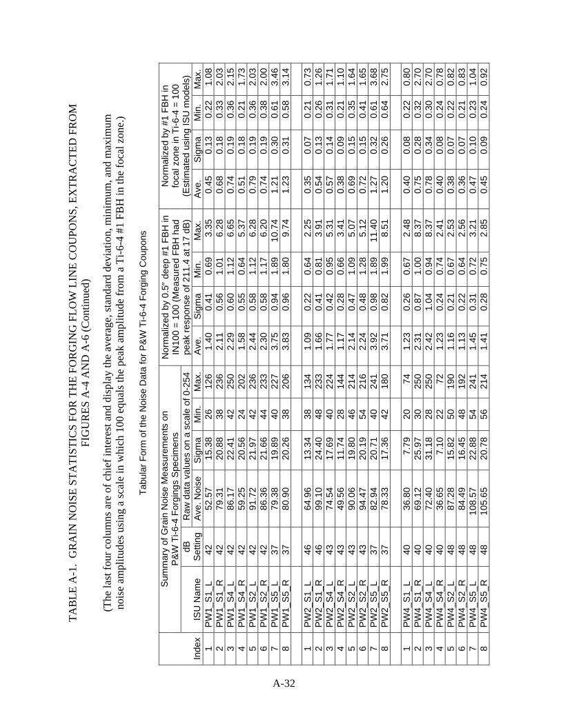
A-32

TAB

LE A

-1.

GR

AIN

NO

ISE

STA

TIST

ICS

FOR

TH

E FO

RG

ING

FLO

W L

INE

CO

UPO

NS,

EX

TRA

CTE

D F

RO

M

FIG

UR

ES A

-4 A

ND

A-6

(Con

tinue

d)

(The

last

four

col

umns

are

of c

hief

inte

rest

and

dis

play

the

aver

age,

stan

dard

dev

iatio

n, m

inim

um, a

nd m

axim

um

nois

e am

plitu

des u

sing

a sc

ale

in w

hich

100

equ

als t

he p

eak

ampl

itude

from

a T

i-6-4

#1

FBH

in th

e fo

cal z

one.

)

Tabu

lar F

orm

of t

he N

oise

Dat

a fo

r P&

W T

i-6-4

For

ging

Cou

pons

Sum

mar

y of

Gra

in N

oise

Mea

sure

men

ts o

n

P&

W T

i-6-4

For

ging

s S

peci

men

s R

aw d

ata

valu

es o

n a

scal

e of

0-2

54

Nor

mal

ized

by

0.5″

dee

p #1

FB

H in

IN

100

= 10

0 (M

easu

red

FBH

had

pe

ak re

spon

se o

f 211

.4 a

t 17

dB)

Nor

mal

ized

by

#1 F

BH

in

foca

l zon

e in

Ti-6

-4 =

100

(E

stim

ated

usi

ng IS

U m

odel

s)

Inde

x IS

U N

ame

dB

Set

ting

Ave

. Noi

se

Sig

ma

Min

. M

ax.

Ave

. S

igm

a M

in.

Max

. A

ve.

Sig

ma

Min

. M

ax.

1 P

W1_

S1_

L 42

52

.57

15.3

8 26

12

6 1.

40

0.41

0.

693.

35

0.45

0.

13

0.22

1.08

2 P

W1_

S1_

R

42

79.3

1 20

.88

38

236

2.11

0.

56

1.01

6.28

0.

68

0.18

0.

332.

033

PW

1_S

4_L

42

86.1

7 22

.41

42

250

2.29

0.

60

1.12

6.65

0.

74

0.19

0.

362.

154

PW

1_S

4_R

42

59

.25

20.5

6 24

20

2 1.

58

0.55

0.

645.

37

0.51

0.

18

0.21

1.73

5 P

W1_

S2_

L 42

91

.72

21.9

7 42

23

6 2.

44

0.58

1.

126.

28

0.79

0.

19

0.36

2.03

6 P

W1_

S2_

R

42

86.3

6 21

.66

44

233

2.30

0.

58

1.17

6.20

0.

74

0.19

0.

382.

007

PW

1_S

5_L

37

79.3

8 19

.89

40

227

3.75

0.

94

1.89

10.7

4 1.

21

0.30

0.

613.

468

PW

1_S

5_R

37

80

.90

20.2

6 38

20

6 3.

83

0.96

1.

809.

74

1.23

0.

31

0.58

3.14

1

PW

2_S

1_L

46

64.9

6 13

.34

38

134

1.09

0.

22

0.64

2.25

0.

35

0.07

0.

210.

732

PW

2_S

1_R

46

99

.10

24.4

0 48

23

3 1.

66

0.41

0.

813.

91

0.54

0.

13

0.26

1.26

3 P

W2_

S4_

L 43

74

.54

17.6

9 40

22

4 1.

77

0.42

0.

955.

31

0.57

0.

14

0.31

1.71

4 P

W2_

S4_

R

43

49.5

6 11

.74

28

144

1.17

0.

28

0.66

3.41

0.

38

0.09

0.

211.

105

PW

2_S

2_L

43

90.0

6 19

.80

46

214

2.14

0.

47

1.09

5.07

0.

69

0.15

0.

351.

646

PW

2_S

2_R

43

94

.47

20.1

9 54

21

6 2.

24

0.48

1.

285.

12

0.72

0.

15

0.41

1.65

7 P

W2_

S5_

L 37

82

.94

20.7

1 40

24

1 3.

92

0.98

1.

8911

.40

1.27

0.

32

0.61

3.68

8 P

W2_

S5_

R

37

78.3

3 17

.36

42

180

3.71

0.

82

1.99

8.51

1.

20

0.26

0.

642.

75

1 P

W4_

S1_

L 40

36

.80

7.79

20

74

1.

23

0.26

0.

672.

48

0.40

0.

08

0.22

0.80

2 P

W4_

S1_

R

40

69.1

2 25

.97

30

250

2.31

0.

87

1.00

8.37

0.

75

0.28

0.

322.

703

PW

4_S

4_L

40

72.4

0 31

.18

28

250

2.42

1.

04

0.94

8.37

0.

78

0.34

0.

302.

704

PW

4_S

4_R

40

36

.65

7.10

22

72

1.

23

0.24

0.

742.

41

0.40

0.

08

0.24

0.78

5 P

W4_

S2_

L 48

87

.28

15.8

2 50

19

0 1.

16

0.21

0.

672.

53

0.38

0.

07

0.22

0.82

6 P

W4_

S2_

R

48

84.4

9 16

.45

48

192

1.13

0.

22

0.64

2.56

0.

36

0.07

0.

210.

837

PW

4_S

5_L

48

108.

57

22.8

8 54

24

1 1.

45

0.31

0.

723.

21

0.47

0.

10

0.23

1.04

8 P

W4_

S5_

R

48

105.

65

20.7

8 56

21

4 1.

41

0.28

0.

752.

85

0.45

0.

09

0.24

0.92

A-33

TAB

LE A

-1.

GR

AIN

NO

ISE

STA

TIST

ICS

FOR

TH

E FO

RG

ING

FLO

W L

INE

CO

UPO

NS,

EX

TRA

CTE

D F

RO

M

FIG

UR

ES A

-4 A

ND

A-6

(Con

tinue

d)

(The

last

four

col

umns

are

of c

hief

inte

rest

and

dis

play

the

aver

age,

stan

dard

dev

iatio

n, m

inim

um, a

nd m

axim

um

nois

e am

plitu

des u

sing

a sc

ale

in w

hich

100

equ

als t

he p

eak

ampl

itude

from

a T

i-6-4

#1

FBH

in th

e fo

cal z

one.

)

Tabu

lar F

orm

of t

he N

oise

Dat

a fo

r P&

W T

i-6-4

For

ging

Cou

pons

Sum

mar

y of

Gra

in N

oise

Mea

sure

men

ts o

n

P&

W T

i-6-4

For

ging

s S

peci

men

s R

aw d

ata

valu

es o

n a

scal

e of

0-2

54

Nor

mal

ized

by

0.5″

dee

p #1

FB

H in

IN

100

= 10

0 (M

easu

red

FBH

had

pe

ak re

spon

se o

f 211

.4 a

t 17

dB)

Nor

mal

ized

by

#1 F

BH

in

foca

l zon

e in

Ti-6

-4 =

100

(E

stim

ated

usi

ng IS

U m

odel

s)

Inde

x IS

U N

ame

dB

Set

ting

Ave

. Noi

se

Sig

ma

Min

. M

ax.

Ave

. S

igm

a M

in.

Max

. A

ve.

Sig

ma

Min

. M

ax.

1 P

W5_

S1_

L 35

33

.93

9.23

18

88

2.

02

0.55

1.

075.

24

0.65

0.

18

0.35

1.69

2 P

W5_

S1_

R

35

84.5

6 26

.53

32

208

5.04

1.

58

1.91

12.3

9 1.

62

0.51

0.

614.

003

PW

5_S

4_L

35

73.4

3 28

.33

24

233

4.37

1.

69

1.43

13.8

8 1.

41

0.54

0.

464.

484

PW

5_S

4_R

35

28

.10

6.73

16

64

1.

67

0.40

0.

953.

81

0.54

0.

13

0.31

1.23

5 P

W5_

S2_

L 41

85

.36

20.0

8 42

20

4 2.

55

0.60

1.

256.

09

0.82

0.

19

0.40

1.96

6 P

W5_

S2_

R

41

81.0

7 20

.05

42

232

2.42

0.

60

1.25

6.92

0.

78

0.19

0.

402.

237

PW

5_S

5_L

41

74.8

5 22

.21

38

246

2.23

0.

66

1.13

7.34

0.

72

0.21

0.

372.

378

PW

5_S

5_R

41

75

.67

19.3

5 40

23

8 2.

26

0.58

1.

197.

10

0.73

0.

19

0.39

2.29

1

PW

6_S

1_L

35

86.8

9 28

.32

36

224

5.17

1.

69

2.14

13.3

4 1.

67

0.54

0.

694.

302

PW

6_S

1_R

35

43

.88

17.1

6 18

16

2 2.

61

1.02

1.

079.

65

0.84

0.

33

0.35

3.11

3 P

W6_

S4_

L 35

34

.29

11.6

16

11

0 2.

04

0.69

0.

956.

55

0.66

0.

22

0.31

2.11

4 P

W6_

S4_

R

35

80.9

2 25

.84

34

244

4.82

1.

54

2.02

14.5

3 1.

55

0.50

0.

654.

695

PW

6_S

2_L

41

72.6

7 17

.13

36

180

2.17

0.

51

1.07

5.37

0.

70

0.16

0.

351.

736

PW

6_S

2_R

41

70

.03

18.5

3 36

20

4 2.

09

0.55

1.

076.

09

0.67

0.

18

0.35

1.96

7 P

W6_

S5_

L 41

59

.19

13.3

1 32

16

6 1.

77

0.40

0.

964.

95

0.57

0.

13

0.31

1.60

8 P

W6_

S5_

R

41

61.3

2 15

.19

34

158

1.83

0.

45

1.01

4.72

0.

59

0.15

0.

331.

52

1 P

W7_

S1_

L 35

42

.6

16.2

8 16

13

0 2.

54

0.97

0.

957.

74

0.82

0.

31

0.31

2.50

2 P

W7_

S1_

R

35

94.0

7 25

.06

42

244

5.60

1.

49

2.50

14.5

3 1.

81

0.48

0.

814.

693

PW

7_S

4_L

35

65.9

5 25

.24

22

210

3.93

1.

50

1.31

12.5

1 1.

27

0.48

0.

424.

034

PW

7_S

4_R

35

26

.27

7.57

14

72

1.

56

0.45

0.

834.

29

0.50

0.

15

0.27

1.38

5 P

W7_

S2_

L 40

98

.16

24.4

9 50

23

8 3.

29

0.82

1.

677.

97

1.06

0.

26

0.54

2.57

6 P

W7_

S2_

R

40

61.8

7 21

.69

22

230

2.07

0.

73

0.74

7.70

0.

67

0.23

0.

242.

487

PW

7_S

5_L

40

37.8

6 9.

63

20

98

1.27

0.

32

0.67

3.28

0.

41

0.10

0.

221.

068

PW

7_S

5_R

40

65

.98

20.9

30

23

8 2.

21

0.70

1.

007.

97

0.71

0.

23

0.32

2.57

A-34

TAB

LE A

-1.

GR

AIN

NO

ISE

STA

TIST

ICS

FOR

TH

E FO

RG

ING

FLO

W L

INE

CO

UPO

NS,

EX

TRA

CTE

D F

RO

M

FIG

UR

ES A

-4 A

ND

A-6

(Con

tinue

d)

(The

last

four

col

umns

are

of c

hief

inte

rest

and

dis

play

the

aver

age,

stan

dard

dev

iatio

n, m

inim

um, a

nd m

axim

um

nois

e am

plitu

des u

sing

a sc

ale

in w

hich

100

equ

als t

he p

eak

ampl

itude

from

a T

i-6-4

#1

FBH

in th

e fo

cal z

one.

)

Tabu

lar F

orm

of t

he N

oise

Dat

a fo

r P&

W T

i-6-4

For

ging

Cou

pons

Sum

mar

y of

Gra

in N

oise

Mea

sure

men

ts o

n

P&

W T

i-6-4

For

ging

s S

peci

men

s R

aw d

ata

valu

es o

n a

scal

e of

0-2

54

Nor

mal

ized

by

0.5″

dee

p #1

FB

H in

IN

100

= 10

0 (M

easu

red

FBH

had

pe

ak re

spon

se o

f 211

.4 a

t 17

dB)

Nor

mal

ized

by

#1 F

BH

in

foca

l zon

e in

Ti-6

-4 =

100

(E

stim

ated

usi

ng IS

U m

odel

s)

Inde

x IS

U N

ame

dB

Set

ting

Ave

. Noi

se

Sig

ma

Min

. M

ax.

Ave

. S

igm

a M

in.

Max

. A

ve.

Sig

ma

Min

. M

ax.

1 P

W8_

S1_

L 35

79

.97

22.8

4 40

22

2 4.

76

1.36

2.

38

13.2

2 1.

54

0.44

0.

77

4.26

2 P

W8_

S1_

R

35

88.2

6 23

.85

44

241

5.26

1.

42

2.62

14

.35

1.70

0.

46

0.85

4.

633

PW

8_S

4_L

33

67.0

5 22

.03

32

227

5.03

1.

65

2.40

17

.02

1.62

0.

53

0.77

5.

494

PW

8_S

4_R

33

69

.79

20.2

32

17

6 5.

23

1.51

2.

40

13.1

9 1.

69

0.49

0.

77

4.26

5 P

W8_

S2_

L 42

73

.38

20.5

9 32

20

8 1.

95

0.55

0.

85

5.53

0.

63

0.18

0.

27

1.78

6 P

W8_

S2_

R

42

46.0

6 10

.81

26

116

1.23

0.

29

0.69

3.

09

0.40

0.

09

0.22

1.

007

PW

8_S

5_L

42

49.5

11

.19

24

138

1.32

0.

30

0.64

3.

67

0.42

0.

10

0.21

1.

188

PW

8_S

5_R

42

62

.11

14.9

1 34

17

4 1.

65

0.40

0.

90

4.63

0.

53

0.13

0.

29

1.49

A-35

TAB

LE A

-1.

GR

AIN

NO

ISE

STA

TIST

ICS

FOR

TH

E FO

RG

ING

FLO

W L

INE

CO

UPO

NS,

EX

TRA

CTE

D F

RO

M

FIG

UR

ES A

-4 A

ND

A-6

(Con

tinue

d)

(The

last

four

col

umns

are

of c

hief

inte

rest

and

dis

play

the

aver

age,

stan

dard

dev

iatio

n, m

inim

um, a

nd m

axim

um

nois

e am

plitu

des u

sing

a sc

ale

in w

hich

100

equ

als t

he p

eak

ampl

itude

from

a T

i-6-4

#1

FBH

in th

e fo

cal z

one.

)

Tabu

lar F

orm

of t

he N

oise

Dat

a fo

r HW

Ti-6

-4 F

orgi

ng C

oupo

ns

S

umm

ary

of G

rain

Noi

se M

easu

rem

ents

on

HW

For

ging

Spe

cim

ens

H1-

H8,

by

C-s

can

“hal

ves”

R

aw d

ata

valu

es o

n a

scal

e of

0 to

0.2

5 V

olts

Nor

mal

ized

by

0.5″

dee

p

#1 F

BH

in IN

100

= 10

0

(afte

r dB

cor

rect

ion)

Nor

mal

ized

by

#1 F

BH

in

foca

l zon

e in

Ti-6

-4 =

100

(E

stim

ated

usi

ng m

odel

s)

Inde

x IS

U N

ame

dB

Set

ting

Ave

. Noi

se

Sig

ma

Min

. M

ax.

Ave

. S

igm

a M

in.

Max

. A

ve.

Sig

ma

Min

. M

ax.

1 H

1_S

1_L

48

0.09

5 0.

014

0.06

30.

160

1.24

0.18

0.

822.

09

0.40

0.

06

0.27

0.67

2 H

1_S

1_R

48

0.

108

0.01

7 0.

068

0.18

2 1.

410.

22

0.89

2.37

0.

45

0.07

0.

290.

773

H1_

S4_

L 48

0.

093

0.01

2 0.

063

0.14

6 1.

210.

16

0.82

1.91

0.

39

0.05

0.

270.

614

H1_

S4_

R

48

0.09

0 0.

012

0.05

50.

170

1.17

0.16

0.

722.

22

0.38

0.

05

0.23

0.72

5 H

1_S

2_L

32

0.05

6 0.

024

0.01

20.

201

4.61

1.98

0.

9916

.55

1.49

0.

64

0.32

5.34

6 H

1_S

2_R

32

0.

053

0.01

9 0.

020

0.13

7 4.

361.

56

1.65

11.2

8 1.

41

0.50

0.

533.

647

H1_

S5_

L 32

0.

049

0.01

8 0.

021

0.19

3 4.

031.

48

1.73

15.8

9 1.

30

0.48

0.

565.

138

H1_

S5_

R

32

0.05

2 0.

016

0.02

30.

137

4.28

1.32

1.

8911

.28

1.38

0.

42

0.61

3.64

1

H2_

S1_

L 36

0.

052

0.01

5 0.

023

0.18

0 2.

640.

76

1.17

9.14

0.

85

0.25

0.

382.

952

H2_

S1_

R

36

0.06

4 0.

025

0.02

70.

234

3.25

1.27

1.

3711

.88

1.05

0.

41

0.44

3.83

3 H

2_S

4_L

38

0.07

5 0.

023

0.03

30.

189

3.02

0.93

1.

337.

62

0.98

0.

30

0.43

2.46

4 H

2_S

4_R

38

0.

058

0.01

6 0.

029

0.16

8 2.

340.

65

1.17

6.78

0.

75

0.21

0.

382.

195

H2_

S2_

L 34

0.

061

0.01

7 0.

031

0.22

9 3.

901.

09

1.98

14.6

4 1.

26

0.35

0.

644.

726

H2_

S2_

R

34

0.05

8 0.

017

0.02

70.

160

3.71

1.09

1.

7310

.23

1.20

0.

35

0.56

3.30

7 H

2_S

5_L

37

0.06

0 0.

015

0.03

30.

180

2.71

0.68

1.

498.

14

0.88

0.

22

0.48

2.63

8 H

2_S

5_R

37

0.

084

0.02

4 0.

035

0.24

2 3.

801.

09

1.58

10.9

5 1.

23

0.35

0.

513.

53

1 H

3_S

1_L

37

0.04

7 0.

016

0.01

60.

135

2.13

0.72

0.

726.

11

0.69

0.

23

0.23

1.97

2 H

3_S

1_R

37

0.

067

0.02

6 0.

025

0.23

0 3.

031.

18

1.13

10.4

1 0.

98

0.38

0.

363.

363

H3_

S4_

L 37

0.

063

0.02

3 0.

029

0.19

9 2.

851.

04

1.31

9.00

0.

92

0.34

0.

422.

904

H3_

S4_

R

37

0.03

6 0.

011

0.01

60.

104

1.63

0.50

0.

724.

71

0.53

0.

16

0.23

1.52

5 H

3_S

2_L

38

0.07

7 0.

022

0.03

70.

199

3.11

0.89

1.

498.

03

1.00

0.

29

0.48

2.59

6 H

3_S

2_R

38

0.

062

0.01

8 0.

031

0.16

2 2.

500.

73

1.25

6.53

0.

81

0.23

0.

402.

117

H3_

S5_

L 38

0.

044

0.01

1 0.

023

0.11

9 1.

770.

44

0.93

4.80

0.

57

0.14

0.

301.

558

H3_

S5_

R

38

0.06

6 0.

018

0.03

30.

182

2.66

0.73

1.

337.

34

0.86

0.

23

0.43

2.37

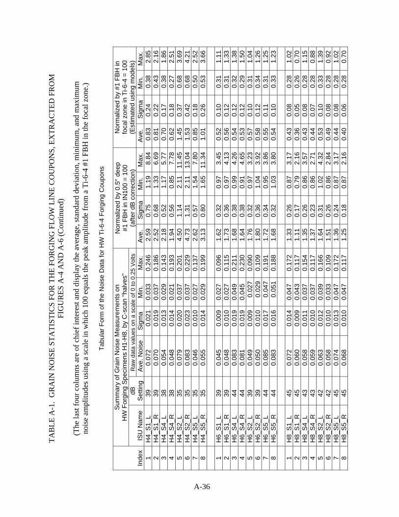
A-36

TAB

LE A

-1.

GR

AIN

NO

ISE

STA

TIST

ICS

FOR

TH

E FO

RG

ING

FLO

W L

INE

CO

UPO

NS,

EX

TRA

CTE

D F

RO

M

FIG

UR

ES A

-4 A

ND

A-6

(Con

tinue

d)

(The

last

four

col

umns

are

of c

hief

inte

rest

and

dis

play

the

aver

age,

stan

dard

dev

iatio

n, m

inim

um, a

nd m

axim

um

nois

e am

plitu

des u

sing

a sc

ale

in w

hich

100

equ

als t

he p

eak

ampl

itude

from

a T

i-6-4

#1

FBH

in th

e fo

cal z

one.

)

Tabu

lar F

orm

of t

he N

oise

Dat

a fo

r HW

Ti-6

-4 F

orgi

ng C

oupo

ns

S

umm

ary

of G

rain

Noi

se M

easu

rem

ents

on

H

W F

orgi

ng S

peci

men

s H

1-H

8, b

y C

-sca

n “h

alve

s”

Raw

dat

a va

lues

on

a sc

ale

of 0

to 0

.25

Vol

ts

Nor

mal

ized

by

0.5″

dee

p #1

FB

H in

IN10

0 =

100

(afte

r dB

cor

rect

ion)

Nor

mal

ized

by

#1 F

BH

in

foca

l zon

e in

Ti-6

-4 =

100

(E

stim

ated

usi

ng m

odel

s)

Inde

x IS

U N

ame

dB

Set

ting

Ave

. Noi

se

Sig

ma

Min

. M

ax.

Ave

. S

igm

a M

in.

Max

. A

ve.

Sig

ma

Min

. M

ax.

1 H

4_S

1_L

39

0.07

2 0.

021

0.03

3 0.

246

2.59

0.

75

1.19

8.

84

0.83

0.

24

0.38

2.

852

H4_

S1_

R

39

0.07

0 0.

019

0.03

7 0.

186

2.52

0.

68

1.33

6.

69

0.81

0.

22

0.43

2.

163

H4_

S4_

L 38

0.

054

0.01

30.

029

0.14

3 2.

18

0.52

1.

17

5.77

0.

70

0.17

0.

38

1.86

4 H

4_S

4_R

38

0.

048

0.01

40.

021

0.19

3 1.

94

0.56

0.

85

7.78

0.

62

0.18

0.

27

2.51

5 H

4_S

2_L

35

0.07

9 0.

020

0.03

7 0.

201

4.50

1.

14

2.11

11

.45

1.45

0.

37

0.68

3.

696

H4_

S2_

R

35

0.08

3 0.

023

0.03

7 0.

229

4.73

1.

31

2.11

13

.04

1.53

0.

42

0.68

4.

217

H4_

S5_

L 35

0.

046

0.01

00.

027

0.13

7 2.

62

0.57

1.

54

7.80

0.

85

0.18

0.

50

2.52

8 H

4_S

5_R

35

0.

055

0.01

40.

029

0.19

9 3.

13

0.80

1.

65

11.3

4 1.

01

0.26

0.

53

3.66

1

H6_

S1_

L 39

0.

045

0.00

90.

027

0.09

6 1.

62

0.32

0.

97

3.45

0.

52

0.10

0.

31

1.11

2 H

6_S

1_R

39

0.

048

0.01

00.

027

0.11

5 1.

73

0.36

0.

97

4.13

0.

56

0.12

0.

31

1.33

3 H

6_S

4_L

44

0.08

3 0.

019

0.04

9 0.

211

1.68

0.

38

0.99

4.

26

0.54

0.

12

0.32

1.

384

H6_

S4_

R

44

0.08

1 0.

019

0.04

5 0.

230

1.64

0.

38

0.91

4.

65

0.53

0.

12

0.29

1.

505

H6_

S2_

L 39

0.

049

0.00

90.

027

0.09

0 1.

76

0.32

0.

97

3.23

0.

57

0.10

0.

31

1.04

6 H

6_S

2_R

39

0.

050

0.01

00.

029

0.10

9 1.

80

0.36

1.

04

3.92

0.

58

0.12

0.

34

1.26

7 H

6_S

5_L

44

0.08

5 0.

017

0.04

70.

191

1.72

0.

34

0.95

3.

86

0.55

0.

11

0.31

1.

258

H6_

S5_

R

44

0.08

3 0.

016

0.05

10.

188

1.68

0.

32

1.03

3.

80

0.54

0.

10

0.33

1.

23

1 H

8_S

1_L

45

0.07

2 0.

014

0.04

7 0.

172

1.33

0.

26

0.87

3.

17

0.43

0.

08

0.28

1.

022

H8_

S1_

R

45

0.06

0 0.

009

0.04

3 0.

117

1.11

0.

17

0.79

2.

16

0.36

0.

05

0.26

0.

703

H8_

S4_

L 43

0.

058

0.01

10.

037

0.15

4 1.

35

0.26

0.

86

3.57

0.

43

0.08

0.

28

1.15

4 H

8_S

4_R

43

0.

059

0.01

00.

037

0.11

7 1.

37

0.23

0.

86

2.71

0.

44

0.07

0.

28

0.88

5 H

8_S

2_L

42

0.06

3 0.

012

0.03

9 0.

166

1.64

0.

31

1.02

4.

32

0.53

0.

10

0.33

1.

396

H8_

S2_

R

42

0.05

8 0.

010

0.03

3 0.

109

1.51

0.

26

0.86

2.

84

0.49

0.

08

0.28

0.

927

H8_

S5_

L 45

0.

074

0.01

30.

047

0.17

2 1.

36

0.24

0.

87

3.17

0.

44

0.08

0.

28

1.02

8 H

8_S

5_R

45

0.

068

0.01

00.

047

0.11

7 1.

25

0.18

0.

87

2.16

0.

40

0.06

0.

28

0.70

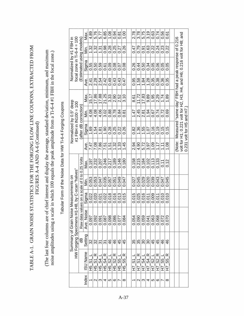
A-37

TAB

LE A

-1.

GR

AIN

NO

ISE

STA

TIST

ICS

FOR

TH

E FO

RG

ING

FLO

W L

INE

CO

UPO

NS,

EX

TRA

CTE

D F

RO

M

FIG

UR

ES A

-4 A

ND

A-6

(Con

tinue

d)

(The

last

four

col

umns

are

of c

hief

inte

rest

and

dis

play

the

aver

age,

stan

dard

dev

iatio

n, m

inim

um, a

nd m

axim

um

nois

e am

plitu

des u

sing

a sc

ale

in w

hich

100

equ

als t

he p

eak

ampl

itude

from

a T

i-6-4

#1

FBH

in th

e fo

cal z

one.

)

Tabu

lar F

orm

of t

he N

oise

Dat

a fo

r HW

Ti-6

-4 F

orgi

ng C

oupo

ns

S

umm

ary

of G

rain

Noi

se M

easu

rem

ents

on

H

W F

orgi

ng S

peci

men

s H

1-H

8, b

y C

-sca

n “h

alve

s”

Raw

dat

a va

lues

on

a sc

ale

of 0

to 0

.25

Vol

ts

Nor

mal

ized

by

0.5″

dee

p

#1 F

BH

in IN

100

= 10

0 (a

fter d

B c

orre

ctio

n)

Nor

mal

ized

by

#1 F

BH

in

foca

l zon

e in

Ti-6

-4 =

100

(E

stim

ated

usi

ng m

odel

s)

Inde

x IS

U N

ame

dB

Set

ting

Ave

. Noi

se

Sig

ma

Min

. M

ax.

Ave

. S

igm

a M

in.

Max

. A

ve.

Sig

ma

Min

. M

ax.

1 H

5_S

1_L

32

0.09

7 0.

022

0.05

30.

197

7.47

1.

69

4.08

15

.17

2.41

0.

55

1.32

4.

89

2 H

5_S

1_R

32

0.

092

0.02

0 0.

053

0.23

2 7.

08

1.54

4.

08

17.8

6 2.

28

0.50

1.

32

5.76

3

H5_

S4_

L 31

0.

091

0.02

1 0.

047

0.20

7 7.

86

1.81

4.

06

17.8

8 2.

54

0.59

1.

31

5.77

4

H5_

S4_

R

31

0.08

7 0.

022

0.03

50.

246

7.51

1.

90

3.02

21

.25

2.42

0.

61

0.98

6.

85

5 H

5_S

2_L

46

0.09

8 0.

018

0.05

70.

217

1.51

0.

28

0.88

3.

33

0.49

0.

09

0.28

1.

08

6 H

5_S

2_R

46

0.

086

0.01

6 0.

051

0.18

9 1.

32

0.25

0.

78

2.90

0.

43

0.08

0.

25

0.94

7

H5_

S5_

L 45

0.

077

0.01

3 0.

049

0.14

6 1.

33

0.22

0.

84

2.52

0.

43

0.07

0.

27

0.81

8

H5_

S5_

R

45

0.08

4 0.

015

0.04

70.

180

1.45

0.

26

0.81

3.

10

0.47

0.

08

0.26

1.

00

1

H7_

S1_

L 35

0.

054

0.01

5 0.

027

0.15

8 2.

94

0.82

1.

47

8.61

0.

95

0.26

0.

47

2.78

2

H7_

S1_

R

35

0.09

0 0.

025

0.04

50.

215

4.90

1.

36

2.45

11

.72

1.58

0.

44

0.79

3.

78

3 H

7_S

4_L

30

0.05

9 0.

016

0.02

90.

184

5.72

1.

55

2.81

17

.83

1.84

0.

50

0.91

5.

75

4 H

7_S

4_R

30

0.

041

0.01

1 0.

020

0.10

2 3.

97

1.07

1.

94

9.89

1.

28

0.34

0.

63

3.19

5

H7_

S2_

L 45

0.

063

0.00

9 0.

039

0.11

3 1.

09

0.16

0.

67

1.95

0.

35

0.05

0.

22

0.63

6

H7_

S2_

R

45

0.06

8 0.

011

0.04

30.

133

1.17

0.

19

0.74

2.

29

0.38

0.

06

0.24

0.

74

7 H

7_S

5_L

46

0.07

2 0.

010

0.04

70.

11

1.11

0.

15

0.72

1.

74

0.36

0.

05

0.23

0.

56

8 H

7_S

5_R

46

0.

070

0.01

0 0.

045

0.12

1.

08

0.15

0.

69

1.89

0.

35

0.05

0.

22

0.61

(Not

e: M

easu

red

“sam

e da

y” F

BH

had

a p

eak

resp

onse

of 0

.216

vo

lt fo

r H1;

0.2

21 v

olt f

or H

2, H

3, H

4, a

nd H

6; 0

.216

vol

t for

H8;

and

0.

231

volt

for H

5 an

d H

7.)

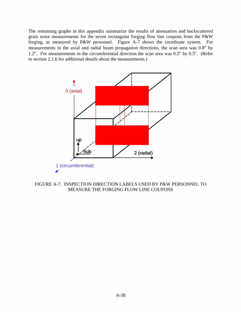
A-38

The remaining graphs in this appendix summarize the results of attenuation and backscattered grain noise measurements for the seven rectangular forging flow line coupons from the P&W forging, as measured by P&W personnel. Figure A-7 shows the coordinate system. For measurements in the axial and radial beam propagation directions, the scan area was 0.8″ by 1.2″. For measurements in the circumferential direction the scan area was 0.5″ by 0.5″. (Refer to section 2.1.6 for additional details about the measurements.)

FIGURE A-7. INSPECTION DIRECTION LABELS USED BY P&W PERSONNEL TO MEASURE THE FORGING FLOW LINE COUPONS

up

hub

1 (circumferential)

2 (radial)

3 (axial)

up

hub

up

hub

1 (circumferential)

2 (radial)

3 (axial)

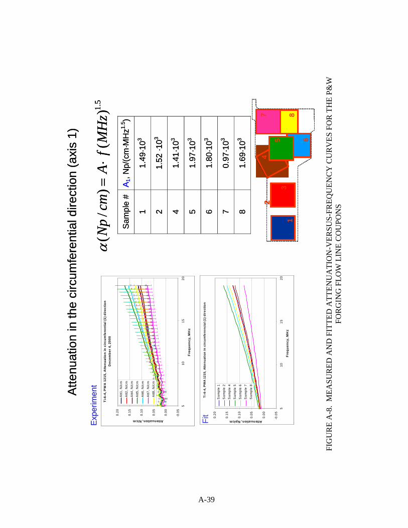
A-39

FI

GU

RE

A-8

. M

EASU

RED

AN

D F

ITTE

D A

TTEN

UA

TIO

N-V

ERSU

S-FR

EQU

ENC

Y C

UR

VES

FO

R T

HE

P&W

FO

RG

ING

FLO

W L

INE

CO

UPO

NS

Atte

nuat

ion

in th

e ci

rcum

fere

ntia

l dire

ctio

n (a

xis

1)

Ti-6

-4, P

WA

121

5, A

tten

uatio

n in

circ

umfe

rent

ial (

1) d

irec

tion

Dec

emb

er 4

, 200

0

-0.0

5

0.00

0.05

0.10

0.15

0.20

510

1520

Fre

quen

cy, M

Hz

Attenuation, N/cm

Att1

, N/c

m

Att2

, N/c

m

Att4

, N/c

mA

tt5, N

/cm

Att6

, N/c

m

Att7

, N/c

m

Att8

, N/c

m

Ti-6

-4, P

WA

1215

, Att

enua

tion

in c

ircu

mfe

renc

ial (

1) d

irec

tion

-0.0

5

0.00

0.05

0.10

0.15

0.20

510

1520

Freq

uen

cy, M

Hz

Attenuation, Np/cm

Sam

ple

1

Sam

ple

2

Sam

ple

4

Sam

ple

5

Sam

ple

6

Sam

ple

7

Sam

ple

8

1.5

(/

)(

)N

pcm

Af

MH

zα

=⋅

Sam

ple

#A 1

, Np/

(cm

·MH

z1.5 )

11.

49·1

03

21.

52 ·1

03

41.

41·1

03

51.

97·1

03

61.

80·1

03

70.

97·1

03

81.

69·1

03

Exp

erim

ent

Fit

1

2

3

4

5 6

7 8

Atte

nuat

ion

in th

e ci

rcum

fere

ntia

l dire

ctio

n (a

xis

1)

Ti-6

-4, P

WA

121

5, A

tten

uatio

n in

circ

umfe

rent

ial (

1) d

irec

tion

Dec

emb

er 4

, 200

0

-0.0

5

0.00

0.05

0.10

0.15

0.20

510

1520

Fre

quen

cy, M

Hz

Attenuation, N/cm

Att1

, N/c

m

Att2

, N/c

m

Att4

, N/c

mA

tt5, N

/cm

Att6

, N/c

m

Att7

, N/c

m

Att8

, N/c

m

Ti-6

-4, P

WA

1215

, Att

enua

tion

in c

ircu

mfe

renc

ial (

1) d

irec

tion

-0.0

5

0.00

0.05

0.10

0.15

0.20

510

1520

Freq

uen

cy, M

Hz

Attenuation, Np/cm

Sam

ple

1

Sam

ple

2

Sam

ple

4

Sam

ple

5

Sam

ple

6

Sam

ple

7

Sam

ple

8

1.5

(/

)(

)N

pcm

Af

MH

zα

=⋅

Sam

ple

#A 1

, Np/

(cm

·MH

z1.5 )

11.

49·1

03

21.

52 ·1

03

41.

41·1

03

51.

97·1

03

61.

80·1

03

70.

97·1

03

81.

69·1

03

Exp

erim

ent

Fit

1

2

3

4

5 6

7 81

2

3

4

5 6

7 8

A-40

FIG

UR

E A

-8.

MEA

SUR

ED A

ND

FIT

TED

ATT

ENU

ATI

ON

-VER

SUS-

FREQ

UEN

CY

CU

RV

ES F

OR

TH

E P&

W

FOR

GIN

G F

LOW

LIN

E C

OU

PON

S (C

ontin

ued)

Atte

nuat

ion

in th

e ra

dial

dire

ctio

n (a

xis

2)

Ti-6

-4, P

WA

121

5, A

tten

uatio

n in

radi

al (2

) dire

ctio

nD

ecem

ber

4, 2

000

-0.0

5

0.00

0.05

0.10

0.15

0.20

510

1520

Fre

que

ncy

, MH

z

Attenuation, N/cm

Att1

, N/c

m

Att2

, N/c

m

Att4

, N/c

m

Att5

, N/c

m

Att6

, N/c

mA

tt7, N

/cm

Att8

, N/c

m

Ti-6

-4, P

WA

121

5, A

tten

uat

ion

in ra

dial

(2) d

irec

tion

-0.0

5

0.00

0.05

0.10

0.15

0.20

510

1520

Fre

qu

ency

, MH

z

Attenuation, Np/cm

Sam

ple

1

Sam

ple

2

Sam

ple

4

Sam

ple

5

Sam

ple

6

Sam

ple

7

Sam

ple

8

1.5

(/

)(

)N

pcm

Af

MH

zα

=⋅

Sam

ple

#A

2, N

p/(c

m·M

Hz1.

5 )

11.

30·1

03

21.

23 ·1

03

41.

34·1

03

51.

77·1

03

61.

66·1

03

71.

16·1

03

81.

41·1

03

Exp

erim

ent

Fit

1

2

3

4

5 6

7 8

Atte

nuat

ion

in th

e ra

dial

dire

ctio

n (a

xis

2)

Ti-6

-4, P

WA

121

5, A

tten

uatio

n in

radi

al (2

) dire

ctio

nD

ecem

ber

4, 2

000

-0.0

5

0.00

0.05

0.10

0.15

0.20

510

1520

Fre

que

ncy

, MH

z

Attenuation, N/cm

Att1

, N/c

m

Att2

, N/c

m

Att4

, N/c

m

Att5

, N/c

m

Att6

, N/c

mA

tt7, N

/cm

Att8

, N/c

m

Ti-6

-4, P

WA

121

5, A

tten

uat

ion

in ra

dial

(2) d

irec

tion

-0.0

5

0.00

0.05

0.10

0.15

0.20

510

1520

Fre

qu

ency

, MH

z

Attenuation, Np/cm

Sam

ple

1

Sam

ple

2

Sam

ple

4

Sam

ple

5

Sam

ple

6

Sam

ple

7

Sam

ple

8

1.5

(/

)(

)N

pcm

Af

MH

zα

=⋅

Sam

ple

#A

2, N

p/(c

m·M

Hz1.

5 )

11.

30·1

03

21.

23 ·1

03

41.

34·1

03

51.

77·1

03

61.

66·1

03

71.

16·1

03

81.

41·1

03

Exp

erim

ent

Fit

1

2

3

4

5 6

7 81

2

3

4

5 6

7 8

A-41

FI

GU

RE

A-8

. M

EASU

RED

AN

D F

ITTE

D A

TTEN

UA

TIO

N-V

ERSU

S-FR

EQU

ENC

Y C

UR

VES

FO

R T

HE

P&W

FO

RG

ING

FLO

W L

INE

CO

UPO

NS

(Con

tinue

d)

Atte

nuat

ion

in th

e ax

ial d

irect

ion

(axi

s 3)

1

2

3

4

5 6

7 8

1.5

(/

)(

)N

pcm

Af

MH

zα

=⋅

Ti-6

-4, P

WA

1215

, Axi

al d

irec

tion

(axi

s 3)

Dec

embe

r 4,

200

0

-0.0

5

0.00

0.05

0.10

0.15

0.20

510

1520

Fre

qu

ency

, MH

z

Attenuation, N/cm

Att1

, N/c

m

Att2

, N/c

m

Att4

, N/c

m

Att5

, N/c

m

Att6

, N/c

m

Att7

, N/c

m

Att8

, N/c

m

Ti-

6-4,

PW

A 1

215,

Axi

al d

ire

ctio

n (

"up"

or

ax

is 3

)

-0.0

5

0.00

0.05

0.10

0.15

0.20

510

1520

Fre

qu

ency

, MH

z

Attenuation, Np/cm

Sam

ple

1

Sam

ple

2

Sam

ple

4

Sam

ple

5

Sam

ple

6

Sam

ple

7

Sam

ple

8

Sam

ple

#A

3, N

p/(c

m·M

Hz1.

5 )

10.

20·1

03

20.

24 ·1

03

40.

72·1

03

51.

00·1

03

61.

07·1

03

70.

75·1

03

82.

07·1

03

Expe

rimen

t

Fit

Atte

nuat

ion

in th

e ax

ial d

irect

ion

(axi

s 3)

1

2

3

4

5 6

7 81

2

3

4

5 6

7 8

1.5

(/

)(

)N

pcm

Af

MH

zα

=⋅

Ti-6

-4, P

WA

1215

, Axi

al d

irec

tion

(axi

s 3)

Dec

embe

r 4,

200

0

-0.0

5

0.00

0.05

0.10

0.15

0.20

510

1520

Fre

qu

ency

, MH

z

Attenuation, N/cm

Att1

, N/c

m

Att2

, N/c

m

Att4

, N/c

m

Att5

, N/c

m

Att6

, N/c

m

Att7

, N/c

m

Att8

, N/c

m

Ti-

6-4,

PW

A 1

215,

Axi

al d

ire

ctio

n (

"up"

or

ax

is 3

)

-0.0

5

0.00

0.05

0.10

0.15

0.20

510

1520

Fre

qu

ency

, MH

z

Attenuation, Np/cm

Sam

ple

1

Sam

ple

2

Sam

ple

4

Sam

ple

5

Sam

ple

6

Sam

ple

7

Sam

ple

8

Sam

ple

#A

3, N

p/(c

m·M

Hz1.

5 )

10.

20·1

03

20.

24 ·1

03

40.

72·1

03

51.

00·1

03

61.

07·1

03

70.

75·1

03

82.

07·1

03

Expe

rimen

t

Fit

A-42

FIG

UR

E A

-9.

MEA

SUR

ED G

RA

IN N

OIS

E FO

M-V

ERSU

S-D

EPTH

CU

RV

ES F

OR

TH

E P&

W F

OR

GIN

G F

LOW

LIN

E C

OU

PON

S, A

ND

A C

OM

PAR

ISO

N O

F M

EASU

RED

VA

LUES

AT

A 2

-cm

DEP

TH

Gra

in n

oise

FO

M a

t 10

MH

z vs

dep

th in

th

e ci

rcum

fere

ntia

l (1)

dire

ctio

n

FOM

Af

=⋅

Cir

cum

fere

ntia

l (1

) di

rect

ion:

FO

M a

t 10

MH

z at

2 c

m

dep

th

0.00

0

0.00

5

0.01

0

0.01

5

0.02

0

0.02

5

0.03

0

1

FOM

-1FO

M-2

FOM

-4FO

M-5

FOM

-6FO

M-7

FOM

-8

Cir

cum

fere

ntia

l (1)

dir

ectio

n: F

OM

vs

dept

h a

t 10

M

Hz

0.00

0.01

0.02

0.03

0.04

0.05

0.06

0.0

1.0

2.0

3.0

4.0

5.0

Dep

th, c

m

FOM, cm^-0.5

FOM

-1

FOM

-2

FOM

-4

FOM

-5

FOM

-6

FOM

-7

FOM

-8

Gra

in n

oise

FO

M a

t 10

MH

z vs

dep

th in

th

e ci

rcum

fere

ntia

l (1)

dire

ctio

n

FOM

Af

=⋅

Cir

cum

fere

ntia

l (1

) di

rect

ion:

FO

M a

t 10

MH

z at

2 c

m

dep

th

0.00

0

0.00

5

0.01

0

0.01

5

0.02

0

0.02

5

0.03

0

1

FOM

-1FO

M-2

FOM

-4FO

M-5

FOM

-6FO

M-7

FOM

-8

Cir

cum

fere

ntia

l (1)

dir

ectio

n: F

OM

vs

dept

h a

t 10

M

Hz

0.00

0.01

0.02

0.03

0.04

0.05

0.06

0.0

1.0

2.0

3.0

4.0

5.0

Dep

th, c

m

FOM, cm^-0.5

FOM

-1

FOM

-2

FOM

-4

FOM

-5

FOM

-6

FOM

-7

FOM

-8

A-43

FIG

UR

E A

-9.

MEA

SUR

ED G

RA

IN N

OIS

E FO

M-V

ERSU

S-D

EPTH

CU

RV

ES F

OR

TH

E P&

W F

OR

GIN

G F

LOW

LIN

E C

OU

PON

S, A

ND

A C

OM

PAR

ISO

N O

F M

EASU

RED

VA

LUES

AT

A 2

-cm

DEP

TH (C

ontin

ued)

Gra

in n

oise

FO

M a

t 10

MH

z vs

dep

th in

th

e ra

dial

(2)d

irect

ion

FOM

Af

=⋅

Rad

ial (

2) d

ire

ctio

n: F

OM

vs

de

pth

at

10 M

Hz

0.00

0.01

0.02

0.03

0.04

0.05

0.06

0.0

0.5

1.0

1.5

2.0

2.5

De

pth

, cm

FOM, cm^-0.5

FOM

-1

FOM

-2

FOM

-4

FOM

-5

FOM

-6

FOM

-7

FOM

-8

Rad

ial (

2) d

irec

tion:

FO

M a

t 10

MH

z at

2 c

m d

epth

0.00

0

0.00

5

0.01

0

0.01

5

0.02

0

0.02

5

0.03

0

1

FOM

-1FO

M-2

FOM

-4FO

M-5

FOM

-6FO

M-7

FOM

-8

Gra

in n

oise

FO

M a

t 10

MH

z vs

dep

th in

th

e ra

dial

(2)d

irect

ion

FOM

Af

=⋅

Rad

ial (

2) d

ire

ctio

n: F

OM

vs

de

pth

at

10 M

Hz

0.00

0.01

0.02

0.03

0.04

0.05

0.06

0.0

0.5

1.0

1.5

2.0

2.5

De

pth

, cm

FOM, cm^-0.5

FOM

-1

FOM

-2

FOM

-4

FOM

-5

FOM

-6

FOM

-7

FOM

-8

Rad

ial (

2) d

irec

tion:

FO

M a

t 10

MH

z at

2 c

m d

epth

0.00

0

0.00

5

0.01

0

0.01

5

0.02

0

0.02

5

0.03

0

1

FOM

-1FO

M-2

FOM

-4FO

M-5

FOM

-6FO

M-7

FOM

-8

A-44

Gra

in n

oise

FO

M a

t 10

MH

z vs

dep

th in

th

e ax

ial (

3)di

rect

ion

FOM

Af

=⋅

Axi

al (

3) d

ire

ctio

n: F

OM

vs

de

pth

at

10 M

Hz

0.00

0.01

0.02

0.03

0.04

0.05

0.06

0.0

0.5

1.0

1.5

2.0

2.5

De

pth

, cm

FOM, cm^-0.5

FOM

-1

FOM

-2

FOM

-4

FOM

-5

FOM

-6

FOM

-7

FOM

-8

Axi

al (3

) dir

ectio

n: F

OM

at 1

0 M

Hz

at 2

cm

dep

th

0.00

0

0.00

5

0.01

0

0.01

5

0.02

0

0.02

5

0.03

0

1

FOM

-1FO

M-2

FOM

-4FO

M-5

FOM

-6FO

M-7

FOM

-8

Gra

in n

oise

FO

M a

t 10

MH

z vs

dep

th in

th

e ax

ial (

3)di

rect

ion

FOM

Af

=⋅

Axi

al (

3) d

ire

ctio

n: F

OM

vs

de

pth

at

10 M

Hz

0.00

0.01

0.02

0.03

0.04

0.05

0.06

0.0

0.5

1.0

1.5

2.0

2.5

De

pth

, cm

FOM, cm^-0.5

FOM

-1

FOM

-2

FOM

-4

FOM

-5

FOM

-6

FOM

-7

FOM

-8

Axi

al (3

) dir

ectio

n: F

OM

at 1

0 M

Hz

at 2

cm

dep

th

0.00

0

0.00

5

0.01

0

0.01

5

0.02

0

0.02

5

0.03

0

1

FOM

-1FO

M-2

FOM

-4FO

M-5

FOM

-6FO

M-7

FOM

-8

FIG

UR

E A

-9.

MEA

SUR

ED G

RA

IN N

OIS

E FO

M-V

ERSU

S-D

EPTH

CU

RV

ES F

OR

TH

E P&

W F

OR

GIN

G F

LOW

LIN

E C

OU

PON

S, A

ND

A C

OM

PAR

ISO

N O

F M

EASU

RED

VA

LUES

AT

A 2

-cm

DEP

TH (C

ontin

ued)

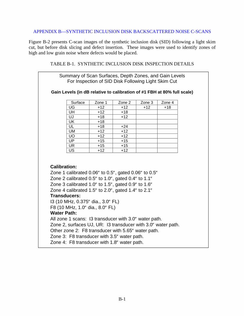
APPENDIX B—SYNTHETIC INCLUSION DISK BACKSCATTERED NOISE C-SCANS

Figure B-2 presents C-scan images of the synthetic inclusion disk (SID) following a light skim cut, but before disk slicing and defect insertion. These images were used to identify zones of high and low grain noise where defects would be placed.

TABLE B-1. SYNTHETIC INCLUSION DISK INSPECTION DETAILS

Summary of Scan Surfaces, Depth Zones, and Gain Levels For Inspection of SID Disk Following Light Skim Cut

Gain Levels (in dB relative to calibration of #1 FBH at 80% full scale)

Surface Zone 1 Zone 2 Zone 3 Zone 4

UG +12 +12 +12 +18 UH +12 +18 UJ +18 +12 UK +18 UL +18 +24 UM +12 +12 UO +12 +12 UP +15 +15 UR +15 +15 US +12 +12

Calibration: Zone 1 calibrated 0.06″ to 0.5″, gated 0.06″ to 0.5″ Zone 2 calibrated 0.5″ to 1.0″, gated 0.4″ to 1.1″ Zone 3 calibrated 1.0″ to 1.5″, gated 0.9″ to 1.6″ Zone 4 calibrated 1.5″ to 2.0″, gated 1.4″ to 2.1″ Transducers: I3 (10 MHz, 0.375″ dia., 3.0″ FL) F8 (10 MHz, 1.0″ dia., 8.0″ FL) Water Path: All zone 1 scans: I3 transducer with 3.0″ water path. Zone 2, surfaces UJ, UR: I3 transducer with 3.0″ water path. Other zone 2: F8 transducer with 5.65″ water path. Zone 3: F8 transducer with 3.5″ water path. Zone 4: F8 transducer with 1.8″ water path.

B-1

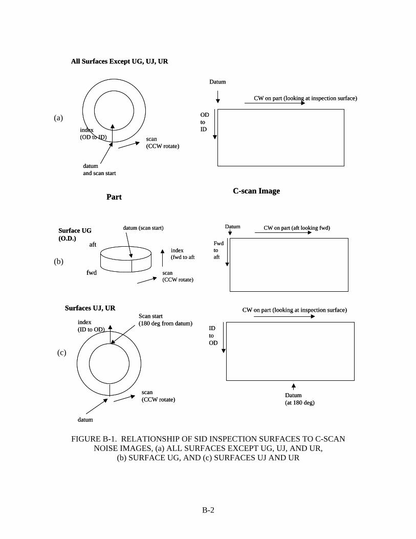
All Surfaces Except UG, UJ, UR

scan(CCW rotate)

index(OD to ID)

Datum

CW on part (looking at inspection surface)

OD to ID

datumand scan start

PartC-scan Image

All Surfaces Except UG, UJ, UR

scan(CCW rotate)

index(OD to ID)

Datum

CW on part (looking at inspection surface)

OD to ID

datumand scan start

PartC-scan Image

Surface UG(O.D.)

aft

fwd scan(CCW rotate)

index(fwd to aft

datum (scan start) Datum CW on part (aft looking fwd)

Fwd to aft

Surface UG(O.D.)

aft

fwd scan(CCW rotate)

index(fwd to aft

datum (scan start) Datum CW on part (aft looking fwd)

Fwd to aft

Surfaces UJ, UR

scan(CCW rotate)

index(ID to OD)

Scan start(180 deg from datum)

Datum(at 180 deg)

CW on part (looking at inspection surface)

ID to OD

datum

Surfaces UJ, UR

scan(CCW rotate)

index(ID to OD)

Scan start(180 deg from datum)

Datum(at 180 deg)

CW on part (looking at inspection surface)

ID to OD

datum

(a)

(b)

(c)

FIGURE B-1. RELATIONSHIP OF SID INSPECTION SURFACES TO C-SCAN

NOISE IMAGES, (a) ALL SURFACES EXCEPT UG, UJ, AND UR, (b) SURFACE UG, AND (c) SURFACES UJ AND UR

B-2

Fwd

Aft

0 60 120 180 240 300 360 degrees CW fromdatum looking at aft face

Region of as-forged surface

Fwd

Aft

Fwd

Aft

0 60 120 180 240 300 3600 60 120 180 240 300 360 degrees CW fromdatum looking at aft face

Region of as-forged surface

C-scan of surface UG, Zone 1. Gain (rel. to #1 FBH) +12 dB, 10 MHz, F/8 transducer, OD side.

FIGURE B-2. C-SCANS OF SID PRIOR TO DEFECT INSERTION

0 60 120 180 240 300 3600 60 120 180 240 300 360

Fwd

Aft

Fwd

Aft

degrees CW fromdatum looking at aft face

C-scan of surface UG, Zone 2. Gain (rel. to #1 FBH) +12 dB, 10 MHz, F/8 transducer, OD side.

FIGURE B-2. C-SCANS OF SID PRIOR TO DEFECT INSERTION (Continued)

B-3

0 60 120 180 240 300 360

Fwd

Aft

degrees CW fromdatum looking at aft face

0 60 120 180 240 300 3600 60 120 180 240 300 360

Fwd

Aft

Fwd

Aft

degrees CW fromdatum looking at aft face

C-scan of surface UG, Zone 3. Gain (rel. to #1 FBH) +12 dB, 10 MHz, F/8 transducer, OD side.

FIGURE B-2. C-SCANS OF SID PRIOR TO DEFECT INSERTION (Continued)

0 60 120 180 240 300 360

Fwd

Aft

degrees CW fromdatum looking at aft face

0 60 120 180 240 300 3600 60 120 180 240 300 360

Fwd

Aft

Fwd

Aft

degrees CW fromdatum looking at aft face

C-scan of surface UG, Zone 4. Gain (rel. to #1 FBH) +12 dB, 10 MHz, F/8 transducer, OD side.

FIGURE B-2. C-SCANS OF SID PRIOR TO DEFECT INSERTION (Continued)

B-4

0 60 120 180 240 300 360

Fwd

Aft

degrees CW fromdatum looking at fwd face

0 60 120 180 240 300 3600 60 120 180 240 300 360

Fwd

Aft

Fwd

Aft

degrees CW fromdatum looking at fwd face

C-scan of surface UH, Zone 1. Gain (rel. to #1 FBH) +12 dB, 10 MHz, F/8 transducer, FWD side.

FIGURE B-2. C-SCANS OF SID PRIOR TO DEFECT INSERTION (Continued)

High noise isreflection from regionof as-forged surface

0 60 120 180 240 300 360

Fwd

Aft

degrees CW fromdatum looking at fwd face

High noise isreflection from regionof as-forged surface

0 60 120 180 240 300 3600 60 120 180 240 300 360

Fwd

Aft

Fwd

Aft

degrees CW fromdatum looking at fwd face

C-scan of surface UH, Zone 2. Gain (rel. to #1 FBH) +18 dB, 10 MHz, F/8 transducer, FWD side.

FIGURE B-2. C-SCANS OF SID PRIOR TO DEFECT INSERTION (Continued)

B-5

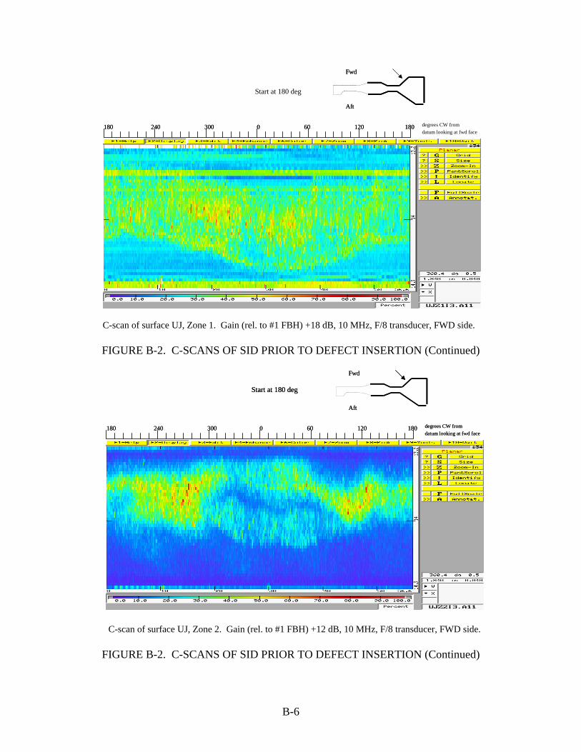
Start at 180 deg

0 60 120180 240 300 1800 60 120180 240 300 180

Fwd

Aft

Fwd

Aft

degrees CW fromdatum looking at fwd face

C-scan of surface UJ, Zone 1. Gain (rel. to #1 FBH) +18 dB, 10 MHz, F/8 transducer, FWD side.

FIGURE B-2. C-SCANS OF SID PRIOR TO DEFECT INSERTION (Continued)

Start at 180 deg

0 60 120180 240 300 180

Fwd

Aft

degrees CW fromdatum looking at fwd face

Start at 180 deg

0 60 120180 240 300 180

Fwd

Aft

degrees CW fromdatum looking at fwd face

C-scan of surface UJ, Zone 2. Gain (rel. to #1 FBH) +12 dB, 10 MHz, F/8 transducer, FWD side.

FIGURE B-2. C-SCANS OF SID PRIOR TO DEFECT INSERTION (Continued)

B-6

0 60 120 180 240 300 360

Fwd

Aft

degrees CW fromdatum looking at fwd face

0 60 120 180 240 300 360

Fwd

Aft

degrees CW fromdatum looking at fwd face

C-scan of surface UK, Zone 1. Gain (rel. to #1 FBH) +18 dB, 10 MHz, F/8 transducer, FWD side.

FIGURE B-2. C-SCANS OF SID PRIOR TO DEFECT INSERTION (Continued)

0 60 120 180 240 300 360

Fwd

Aft

degrees CW fromdatum looking at fwd face

0 60 120 180 240 300 3600 60 120 180 240 300 360

Fwd

Aft

Fwd

Aft

degrees CW fromdatum looking at fwd face

C-scan of surface UL, Zone 1. Gain (rel. to #1 FBH) +18 dB, 10 MHz, F/8 transducer, FWD side.

FIGURE B-2. C-SCANS OF SID PRIOR TO DEFECT INSERTION (Continued)

B-7

0 60 120 180 240 300 360

Fwd

Aft

degrees CW fromdatum looking at fwd face

0 60 120 180 240 300 3600 60 120 180 240 300 360

Fwd

Aft

Fwd

Aft

degrees CW fromdatum looking at fwd face

C-scan of surface UL, Zone 2. Gain (rel. to #1 FBH) +24 dB, 10 MHz, F/8 transducer, FWD side.

FIGURE B-2. C-SCANS OF SID PRIOR TO DEFECT INSERTION (Continued)

0 60 120 180 240 300 360

Fwd

Aft

degrees CW fromdatum looking at fwd face

0 60 120 180 240 300 3600 60 120 180 240 300 360

Fwd

Aft

Fwd

Aft

degrees CW fromdatum looking at fwd face

C-scan of surface UM, Zone 1. Gain (rel. to #1 FBH) +12 dB, 10 MHz, F/8 transducer, FWD side.

FIGURE B-2. C-SCANS OF SID PRIOR TO DEFECT INSERTION (Continued)

B-8

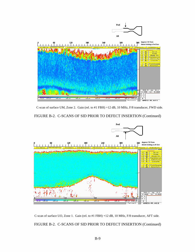
0 60 120 180 240 300 360

Fwd

Aft

degrees CW fromdatum looking at fwd face

0 60 120 180 240 300 3600 60 120 180 240 300 360

Fwd

Aft

Fwd

Aft

degrees CW fromdatum looking at fwd face

C-scan of surface UM, Zone 2. Gain (rel. to #1 FBH) +12 dB, 10 MHz, F/8 transducer, FWD side.

FIGURE B-2. C-SCANS OF SID PRIOR TO DEFECT INSERTION (Continued)

0 60 120 180 240 300 360

Fwd

Aft

degrees CW fromdatum looking at aft face

0 60 120 180 240 300 3600 60 120 180 240 300 360

Fwd

Aft

Fwd

Aft

degrees CW fromdatum looking at aft face

C-scan of surface UO, Zone 1. Gain (rel. to #1 FBH) +12 dB, 10 MHz, F/8 transducer, AFT side.

FIGURE B-2. C-SCANS OF SID PRIOR TO DEFECT INSERTION (Continued)

B-9

0 60 120 180 240 300 360

Fwd

Aft

degrees CW fromdatum looking at aft face

0 60 120 180 240 300 3600 60 120 180 240 300 360

Fwd

Aft

Fwd

Aft

degrees CW fromdatum looking at aft face

C-scan of surface UO, Zone 2. Gain (rel. to #1 FBH) +12 dB, 10 MHz, F/8 transducer, AFT side.

FIGURE B-2. C-SCANS OF SID PRIOR TO DEFECT INSERTION (Continued)

0 60 120 180 240 300 360

Fwd

Aft

degrees CW fromdatum looking at aft face

0 60 120 180 240 300 3600 60 120 180 240 300 360

Fwd

Aft

Fwd

Aft

degrees CW fromdatum looking at aft face

C-scan of surface UP, Zone 1. Gain (rel. to #1 FBH) +15 dB, 10 MHz, F/8 transducer, AFT side.

FIGURE B-2. C-SCANS OF SID PRIOR TO DEFECT INSERTION (Continued)

B-10

0 60 120 180 240 300 360

Fwd

Aft

degrees CW fromdatum looking at aft face

0 60 120 180 240 300 3600 60 120 180 240 300 360

Fwd

Aft

Fwd

Aft

degrees CW fromdatum looking at aft face

C-scan of surface UP, Zone 2. Gain (rel. to #1 FBH) +15 dB, 10 MHz, F/8 transducer, AFT side.

FIGURE B-2. C-SCANS OF SID PRIOR TO DEFECT INSERTION (Continued)

Start at 180 deg

0 60 120180 240 300 180

Fwd

Aft

degrees CW fromdatum looking at aft face

Start at 180 deg

0 60 120180 240 300 1800 60 120180 240 300 180

Fwd

Aft

Fwd

Aft

degrees CW fromdatum looking at aft face

C-scan of surface UR, Zone 1. Gain (rel. to #1 FBH) +15 dB, 10 MHz, F/8 transducer, AFT side.

FIGURE B-2. C-SCANS OF SID PRIOR TO DEFECT INSERTION (Continued)

B-11

0 60 120180 240 300 180

Fwd

Aft

degrees CW fromdatum looking at aft face

0 60 120180 240 300 1800 60 120180 240 300 180

Fwd

Aft

Fwd

Aft

degrees CW fromdatum looking at aft face

C-scan of surface UR, Zone 2. Gain (rel. to #1 FBH) +15 dB, 10 MHz, F/8 transducer, AFT side.

FIGURE B-2. C-SCANS OF SID PRIOR TO DEFECT INSERTION (Continued)

0 60 120 180 240 300 360

Fwd

Aft

degrees CW fromdatum looking at aft face

0 60 120 180 240 300 3600 60 120 180 240 300 360

Fwd

Aft

degrees CW fromdatum looking at aft face

C-scan of surface US, Zone 1. Gain (rel. to #1 FBH) +12 dB, 10 MHz, F/8 transducer, AFT side.

FIGURE B-2. C-SCANS OF SID PRIOR TO DEFECT INSERTION (Continued)

B-12

0 60 120 180 240 300 360

Fwd

Aft

degrees CW fromdatum looking at aft face

0 60 120 180 240 300 3600 60 120 180 240 300 360

Fwd

Aft

Fwd

Aft

degrees CW fromdatum looking at aft face

C-scan of surface US, Zone 2. Gain (rel. to #1 FBH) +12 dB, 10 MHz, F/8 transducer, AFT side.

FIGURE B-2. C-SCANS OF SID PRIOR TO DEFECT INSERTION (Continued)

B-13/B-14

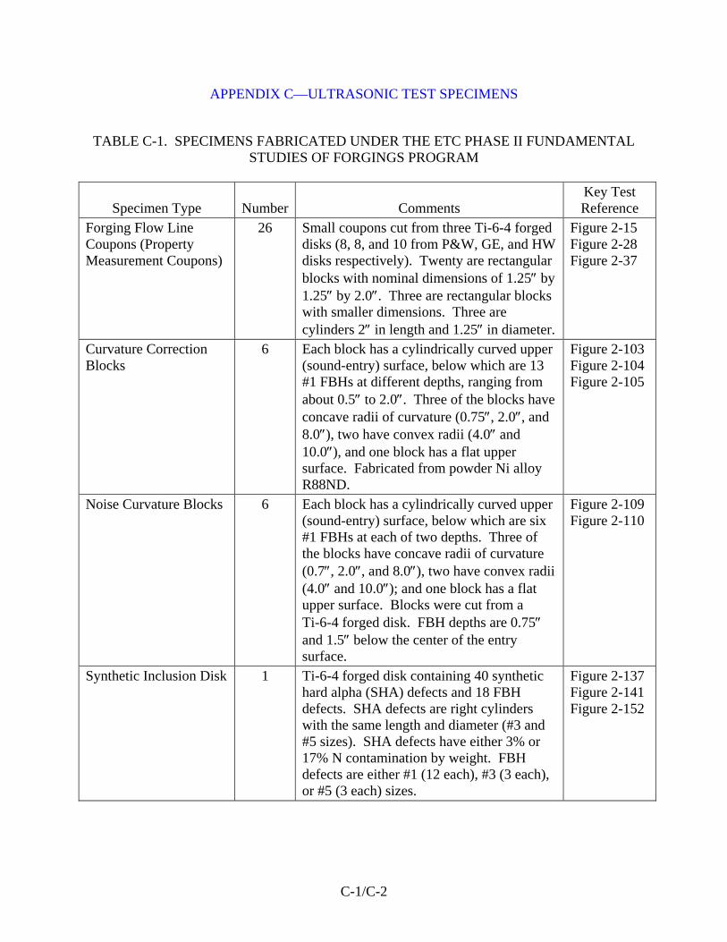
APPENDIX C—ULTRASONIC TEST SPECIMENS

TABLE C-1. SPECIMENS FABRICATED UNDER THE ETC PHASE II FUNDAMENTAL

STUDIES OF FORGINGS PROGRAM

Specimen Type Number Comments Key Test Reference

Forging Flow Line Coupons (Property Measurement Coupons)

26 Small coupons cut from three Ti-6-4 forged disks (8, 8, and 10 from P&W, GE, and HW disks respectively). Twenty are rectangular blocks with nominal dimensions of 1.25″ by 1.25″ by 2.0″. Three are rectangular blocks with smaller dimensions. Three are cylinders 2″ in length and 1.25″ in diameter.

Figure 2-15 Figure 2-28 Figure 2-37

Curvature Correction Blocks

6 Each block has a cylindrically curved upper (sound-entry) surface, below which are 13 #1 FBHs at different depths, ranging from about 0.5″ to 2.0″. Three of the blocks have concave radii of curvature (0.75″, 2.0″, and 8.0″), two have convex radii (4.0″ and 10.0″), and one block has a flat upper surface. Fabricated from powder Ni alloy R88ND.

Figure 2-103 Figure 2-104 Figure 2-105

Noise Curvature Blocks 6 Each block has a cylindrically curved upper (sound-entry) surface, below which are six #1 FBHs at each of two depths. Three of the blocks have concave radii of curvature (0.7″, 2.0″, and 8.0″), two have convex radii (4.0″ and 10.0″); and one block has a flat upper surface. Blocks were cut from a Ti-6-4 forged disk. FBH depths are 0.75″ and 1.5″ below the center of the entry surface.

Figure 2-109 Figure 2-110

Synthetic Inclusion Disk 1 Ti-6-4 forged disk containing 40 synthetic hard alpha (SHA) defects and 18 FBH defects. SHA defects are right cylinders with the same length and diameter (#3 and #5 sizes). SHA defects have either 3% or 17% N contamination by weight. FBH defects are either #1 (12 each), #3 (3 each), or #5 (3 each) sizes.

Figure 2-137 Figure 2-141 Figure 2-152

C-1/C-2