dot asia pacific 2008 - eca pipeline rev 3 1

A Methodology for Engineering Criticality Assessment (ECA) for Offshore Pipelines

Ben Lee PhD, J P Kenny, Inc.

Paul Jukes PhD, J P Kenny, Inc.

Ayman Eltaher PhD PE, J P Kenny, Inc.

James Wang MSc, J P Kenny, Inc.

J P Kenny, Inc.

15115 Park Row, Houston, TX 77084

Abstract

This paper presents a methodology for an Engineering Criticality Assessment (ECA), and

results from a study, for the flaws in the welded joints of gas export offshore pipelines.

The ECA analyses were performed based on the assumption of various concrete

stiffnesses, which considers full concrete stiffness and some degree of concrete stiffness

degradation during the service. A series of field surveys were conducted to assess the

existing defect sizes, joint KP, field joint number, weld number, pipe/seabed profile, TDP

location, span length and water depth, etc. Based on the survey data, finite element model

was developed using ABAQUS to calculate the natural frequencies, stresses and mode

shapes. The in-house MathCad spreadsheet was developed based on DNV-RP-F105 to

generate stress ranges. The results obtained from ABAQUS and MathCad program were

used as an input data to ECA analysis. The new technology in this paper is the use of

advanced finite element analysis tools to determine the inputs for the ECA.

In order to determine the maximum allowable flaw sizes at critical weld locations under

operating and extreme environmental load conditions, TWI software Crackwise 4 was

used in the assessment. Crackwise 4 is a Windows based integrated software package,

which automates the fracture and fatigue assessment procedures based on BS 7910:2005.

For fracture and fatigue analysis of pipelines, a level 2 analysis was conducted using the

stress concentration factor and reference stress solution. The ECA assessment assumed a

welding residual stress condition allowing relaxation and different stress concentration

factors due to weld misalignment. The acceptance criteria were developed under extreme

environmental load condition as a guideline. The final flaw sizes induced from the fatigue

analyses were compared with the established acceptance criteria to assure the structural

integrity of the pipelines. The survey assessed weld defect sizes were also compared with

the acceptance criteria to make an engineering decision for fitness-for-service.

Keywords: DNV (Det Norske Veritas); ULS (Ultimate Limit State); FLS (Fatigue Limit

State); WIF (Wave Induced Fatigue); FM (Force Model); VIV (Vortex Induced

Vibration); RM (Response Model); Mode Shape; Natural Frequency; Unit Stress; CSF

(Concrete Stiffness Factor); ECA (Engineering Critical Assessment); FAD (Failure

Assessment Diagram); CTOD (Crack Tip Opening Displacement); NDE (Non-

destructive Evaluation); AUT (Automated Ultrasonic Testing); TWI (The Welding

Institute)

1. Introduction

Offshore pipelines which have been damaged locally due to the free spanning may not

satisfy its intended design life. The pipeline integrity assessment is very important;

however, analysis procedures may be complicated because of the interpretation of

surveyed data, and application of the advanced tools. Correct interpretation of surveyed

data such as wave/current, soil properties, single span and interacting span, stiffness of

pipeline, residual tension and interaction between pipe and soil etc is critically important

in order to estimate accurate strength and fatigue life.

Free spanning analysis procedures are specified in DNV-RP-F105 for strength and

fatigue evaluation due to in-line and cross-flow Vortex Induced Vibration (VIV) and

direct wave loading. The detailed fatigue analysis is based on the S-N curve method

which is a quick and reliable method; however, S-N curve method cannot reflect the

pipeline static strength degradation with service. Any free spanning pipelines may be able

to withstand the extreme storm condition as long as the accumulated fatigue damage is

below unity (1.0). The fatigue life of offshore pipelines consists of both crack initiation

and crack propagation life. Since the crack propagation life is affected by the pipeline

static strength which decreases with the crack propagation, the static strength assessment

is an integral part of the analysis. Welding induced defects or propagated cracks may be

large enough to fail the free spanning pipelines under design extreme condition which

cannot be considered in the conventional S-N curve method. In order to include the

welding defects or grown fatigue cracks in the assessment of structural integrity of free

spanning pipelines, Engineering Criticality Assessment (ECA) software, Crackwise, was

adopted as well as advanced finite element tool such as ABAQUS. In-house program was

also developed to better align with industry standard practices such as DNV-RP-F105 and

DNV-OS-F101. This paper presents a methodology from the screening analysis to ECA

analysis to assess the integrity of offshore pipelines with the use of advanced finite

element tools.

2. Assessment of Free Spanning Pipelines

Free spanning pipeline analyses was performed based on DNV-RP-F105. A span survey

data was assessed initially to prepare all the necessary input data in order to perform

static and dynamic ULS (Ultimate Limit State) checks based on DNV-OS-F101. A VIV

screening analysis was then conducted to determine the maximum allowable span length

for in-line and cross-flow directions under both current and wave conditions. Finally a

fatigue analysis was performed for the spans that exceed the maximum allowable span

length.

2.1 Field Data Assessment

Field survey data were assessed and these raw data were processed in order to eliminate

noise and invalid data before use in the FEA modeling, screening determination and

fatigue life calculation. The assessment is performed yearly basis to accommodate the

variation of field data. The key survey data are described as follows:

• Free span length

• Span location

• Height (gap) between the pipeline and seabed

• Pipe profiles

• Touchdown point

• Wave / current data with associated number of occurrences

• Wave / current directions

• Soil data

• Seabed profiles

Perpendicular interactions between wave/current and pipeline are assumed for

conservative results if directional information is not available.

2.2 Screening Analysis

The environmental data, water depth, concrete coating thickness and free span length

would be different along the pipeline sections. The purpose of screening analysis is to

define a criterion that is applied to free spans in order to capture any free spans which

exceed screening criteria. The most onerous spans can be prioritized for detailed analysis.

The maximum allowable span lengths are normally determined in the screening analysis

by VIV onsets at both inline and crossflow directions defined in DNV-RP-F105 and by

assuming ULS unity of 1 based on the procedures described in DNV-OS-F101. The

pipeline route is divided into several sections to accommodate different concrete coating

thickness, water depth and environmental data. In each section, an average water depth

was selected and maximum environmental data was applied for conservative analysis.

The following governing criteria were used to calculate the maximum allowable span

lengths:

• Fatigue due to in-line VIV

• Fatigue due to cross-flow VIV

• Static ULS check

• Dynamic ULS check

The screening analysis was performed using the in-house spreadsheet which considers

the following features:

• Static load, VIV load and direct wave load were considered in the calculation.

• Boundary condition: “single span on seabed” is used for a single span, and the

“pinned-pinned” is used for interactive spans. Based on DNV-RP-F105, the

effective span length is used only for the “single span” case. For the interacting

span case with “pinned-pinned”, the apparent span length is used. The effective

span length is defined as the equivalent length considering soil stiffness and

boundary conditions. The apparent span length is the original span length

identified based on the seabed profile and pipeline information.

• The maximum gap is used in the screening analysis for conservative results.

The determination of single and interacting spans is based on the initial survey data and

engineering judgment. A single span boundary condition is assumed when the pipe is

fully embedded into the soil at the span shoulders. The interacting span barely touches

the soil (less than 0.5 meters) at one end of the pipe. Alternative ways to distinguish

between the single and interactive span is to use the free span classification defined in

DNV-RP-F105. In some cases, a screening analysis was performed based on the

assumption of interacting span boundary conditions in order to generate conservative

allowable span lengths.

2.3 FEA Modeling

The code base calculation of natural frequency and unit stresses may be enough during

the screening analysis because code base results are usually conservative. A finite

element analysis is necessary in order to apply more accurate loads and boundary

conditions and calculate more accurate natural frequency and combined unit stresses

under various vibration modes. Non-linear finite element software, ABAQUS was used

in the analysis.

2.3.1 Pipe Element

The 2-node pipe element was used in the analysis. Initially element size of 1 meter was

used and had been fine meshed via iteration based on span length and higher order modes.

2.3.2 Loads and Boundary Conditions

ULS checks are considering environmental loading of 100 year current/1 year wave or 1

year current/100 year wave. Both environmental cases are checked and governing ULS

values are selected as a result. For fatigue analysis, flow conditions due to current and

wave action at the pipe level govern the response of free spanning pipeline. The steady

current velocity and wave-induced flow velocity are added together with relevant

probability of occurrence for each velocity.

In a screening analysis, boundary conditions are applied as specified in DNV-RP-F105. It

may not represent actual boundary conditions; therefore, it is only applied during the

screening analysis.

In order to mimic the interactions between the pipe and soil in FE analysis, a contact

model is used in the static analysis and the spring model is used in the dynamic analysis.

A contact model includes two contact surfaces, the pipe surface and seabed surface. The

pipe surface is generated from the pipe elements and act as a slave surface and seabed

surface is defined as a rigid body with the stiffness between the pipe and soil and act as a

mater surface. In the contact model, linear stiffness is used to consider the vertical

direction boundary conditions and constant friction factors are used to accommodate the

pipe and soil interaction. Both soil stiffness and friction factors can be obtained from

DNV-RP-F105. In the spring model, non-linear spring elements are applied to the nodes

between pipe and seabed in axial, lateral and vertical directions.

2.3.3 Concrete Modeling

The concrete was modeled as an outer pipe relative to the steel pipe using pipe-in-pipe

(PIP) model. The concrete and pipe are bonded together right after installation and

representing intact condition which has full concrete bending stiffness. Large bending

strains are generated at span area which induce cracks in the concrete and reduce bending

stiffness of concrete. Some degree of concrete stiffness degradation during the service is

considered in the analysis.

The discontinuity of concrete coating at the field joint was considered by applying stress

concentration factor (SCF) using the equation defined below. The equation has been

calibrated using the separate FEA model and applied to ULS checks and fatigue

calculation.

75.0

1

+=

steel

conc

EI

EISCF (1)

where,

EIconc : Young’s Modulus and Inertia of Concrete Coating

EIsteel : Young’s Modulus and Inertia of Steel Pipe

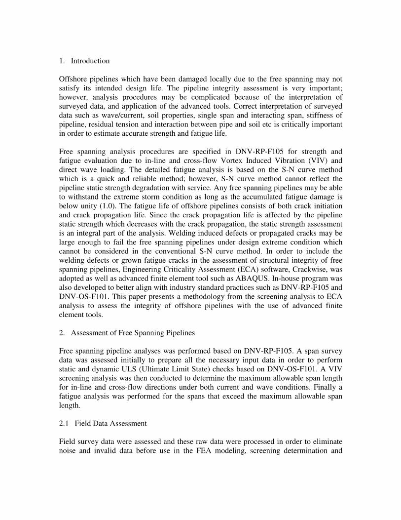
2.4 ULS Check

The purpose of ULS check is to ensure the pipeline is within the corresponding pipeline

specification limit by using more accurate results such as natural frequency and unit

stress obtained from the FEA. The ULS calculation is performed based on the DNV-OS-

F101 using the extreme environmental loading conditions. The loads used in the

calculation are the following:

• Static load – weight

• VIV loads from in-line and cross flow vibrations

• Direct wave load – direct drag and inertia effects

An example of the ULS check results along the pipeline length is shown in Figure 2.1.

Unit Check Results

0.00

0.10

0.20

0.30

0.40

0.50

0.60

0.70

0.80

0.90

1.00

0 50 100 150 200 250 300 350 400

Pipeline Length, m

Un

it C

he

ck

Re

su

lts

Figure 2.1 Unit check results along the pipeline length

2.5 Fatigue Calculation Procedures

Similar to the span screening analysis, fatigue analysis is conducted for each span

corresponding to the applicable changes in concrete coating thickness, seabed topography,

water depth, span gap and environmental data. In the fatigue analysis, static load, VIV

loads and direct wave loads are considered in the calculation. The wave information

contains 8 significant wave heights, 20 periods and 8 directions with relevant

probabilities. The current information contains 8 directions with relevant probabilities.

The span gap is calculated as average value over the central third of the span suggested

by DNV-RP-F105.

For fatigue life assessment, both “Response Model” and “Force Model” are used in the

calculation. In the “Response Model”, both the in-line and cross-flow are considered in

the current and wave induced VIV. For the “Force Model”, the calculation is based on

Morison’s equation for direct in-line loading.

2.5.1 Natural Frequency Determination

The natural frequency and mode shapes are calculated from the FE analysis to perform

accurate fatigue life calculation. The soil stiffness, residual lay tension and concrete

stiffness are input parameters for FE analysis. If residual tension is not available for

existing pipeline, tension may be determined by trial and error. The pipeline profile

measured by survey data can be matched with FE predicted pipeline static profile by

changing the residual tension. The pipeline mid-point is selected and predicted span

height and surveyed span height are compared. If the difference of these span heights at

the mid-point is within a certain limit (∆1 and ∆2 in Fig. 2.2), it is assumed that pipeline

profile matching is achieved and residual tension is selected. Alternatively, the averaged

differences between the predicted span height and the surveyed span height along the

span length are also used as the match criteria.

Fig. 2.2: Pipe Profile Comparison

The soil stiffness is assessed based on the DNV codes. Depending on the pipe size and

the total weight, the dynamic soil stiffness can vary with one location to another, mostly

due to the variation in concrete thickness.

To ensure a conservative estimate of the residual lay tension, sensitivity studies are

performed to determine a range of residual tension that produces a matching pipeline

profile. The sensitivity study accounts for the uncertainty due to soil properties, concrete

conditions (intact or damaged), and survey accuracy. The range of the parameters is

initially taken as the following:

• The soil static stiffness: nominal +/- tolerance in a certain percentage

• Survey accuracy: (height) +/- tolerance

• Concrete condition – Young’s modulus: nominal +/- tolerance

The tolerance for each item varies from case to case, thereby varying the inputs. As a

result, a range of tension and frequency values are calculated and is used in the

subsequent fatigue analysis.

2.5.2 S-N Fatigue Software

The environmental data and FE results are used as an input data to DNV FatFree software

version 10 and fatigue life was calculated for the span. In the FatFree software, the

following features are included:

• Current and wave modules accounting for the current and wave effects in VIV

• Force model calculations for direct wave load response

• Multimode response for VIV calculations

• Fully compatible with DNV-RP-F105

Several primary parameters that influence the fatigue life in general are the natural

frequencies, mode shapes, span lengths, current / wave data, water depth and weld type

etc.

If any crack is initiated during the service and propagated to a certain size due to the

cyclic stresses, ECA is necessary to make an engineering judgment whether it is

acceptable or not for the continuing service. The schematic diagrams of overall

calculation procedures from the screening analysis to ECA analysis are described in

Figure A1 of Appendix A.

3. ECA for Offshore Pipelines

The objective of the Engineering Critical Assessment (ECA) is to determine the

maximum allowable flaw sizes for surface and embedded flaws in the weld metal of

pipelines under operating and extreme loadings. The acceptance criteria were developed

under extreme environmental load condition as a guideline. The final flaw sizes induced

from the fatigue analyses were compared with the established acceptance criteria to

assure the structural integrity of the pipelines. The survey assessed weld defect sizes were

also compared with the acceptance criteria to make an engineering decision for fitness-

for-service.

3.1 Analysis Procedure

Two spans at KP “A” and KP “B” are analyzed to output the stress ranges for ECA

analysis. The results are based on the metocean data with wave directionality, and one-

year near-bottom extreme current.

A flow chart for stress range calculation procedures are shown in Figure 3.1. The

calculation procedures for stress ranges are described as follows:

1. Input data (pipeline parameters, DNV-RP-F105 parameters, environmental

parameters, metocean parameters)

2. Structure calculations (pipe submerged weight, inertia moment etc.)

3. Soil calculation

4. Environmental calculations (wave induced velocity, current velocity at pipe

location)

5. Response Model (RM)

6. Force Model (FM)

7. Stress range output (stress ranges from RM and FM)

This calculation procedure is a DNV-RP-F105 code based calculation using FE results.

In-line VIV, cross-flow VIV, and in-line direct wave loading are considered in the

analysis. The stress ranges from in-line / cross-flow VIV and direct wave load are

required for ECA. DNV FatFree software generates span fatigue life only and related

stress ranges are not available from FatFree. Therefore, in-house program was developed

to generate stress ranges and number of vibration cycles per year based on the Response

Model and Force Model.

Figure 3.1 Flow Chart for Stress Range Calculation

Stress histograms are obtained at two (2) critical locations; KP “A” and KP “B” in the

pipeline. Crack growth assessment shall consider cyclic stress histograms determined

from wave induced fatigue (WIF) analysis and vortex induced vibration (VIV) analysis.

The analysis was performed with an assumption of full concrete stiffness and 30%

concrete stiffness degradation. The current and wave induced flow components are

assumed co-linear as DNV-RP-F105 indicated. The directional probability of occurrence

data for waves is used in the analysis.

3.2 Analysis Type

The ECA was performed in accordance with BS 7910:2005 using Level 2A analysis.

Generalized Failure Assessment Diagram (FAD) option was selected to characterize the

mechanical behavior of weld metal as actual stress and strain curve data for the weld

metal was not available.

3.3 ECA Software

Start

ABAQUS/FEA: Natural Frequency Mode Shape

Excel Spreadsheet: Equivalent Stress Factor

Stress Range Cycles per Year (Force Model)

Stop

DNV-RP-F105 (2006): Section 5.2.7

Stress Range Cycles per Year (Response Model)

Stress Ranges and Cycles

The ECA was performed using TWI software Crackwise 4.0. Crackwise is a Windows

based integrated software package, which automates the fracture and fatigue assessment

procedures in the BS 7910:2005.

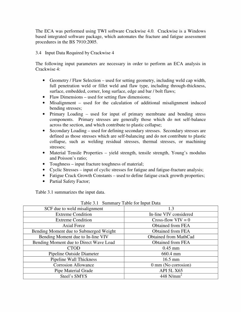
3.4 Input Data Required by Crackwise 4

The following input parameters are necessary in order to perform an ECA analysis in

Crackwise 4:

• Geometry / Flaw Selection – used for setting geometry, including weld cap width,

full penetration weld or fillet weld and flaw type, including through-thickness,

surface, embedded, corner, long surface, edge and bar / bolt flaws;

• Flaw Dimensions – used for setting flaw dimensions;

• Misalignment – used for the calculation of additional misalignment induced

bending stresses;

• Primary Loading – used for input of primary membrane and bending stress

components. Primary stresses are generally those which do not self-balance

across the section, and which contribute to plastic collapse;

• Secondary Loading – used for defining secondary stresses. Secondary stresses are

defined as those stresses which are self-balancing and do not contribute to plastic

collapse, such as welding residual stresses, thermal stresses, or machining

stresses;

• Material Tensile Properties – yield strength, tensile strength, Young’s modulus

and Poisson’s ratio;

• Toughness – input fracture toughness of material;

• Cyclic Stresses – input of cyclic stresses for fatigue and fatigue-fracture analysis;

• Fatigue Crack Growth Constants – used to define fatigue crack growth properties;

• Partial Safety Factor;

Table 3.1 summarizes the input data.

Table 3.1 Summary Table for Input Data

SCF due to weld misalignment 1.3

Extreme Condition In-line VIV considered

Extreme Condition Cross-flow VIV = 0

Axial Force Obtained from FEA

Bending Moment due to Submerged Weight Obtained from FEA

Bending Moment due to In-line VIV Obtained from MathCad

Bending Moment due to Direct Wave Load Obtained from FEA

CTOD 0.45 mm

Pipeline Outside Diameter 660.4 mm

Pipeline Wall Thickness 16.5 mm

Corrosion Allowance 0 mm (No corrosion)

Pipe Material Grade API 5L X65

Steel’s SMYS 448 N/mm2

Steel’s SMTS 531 N/mm2

Steel’s Modulus of Elasticity 207000 N/mm2

External Corrosion Coat (FBE) Thickness 0.4 mm

Concrete Coating Thickness 60 mm

Concrete Elastic Modulus 3.13E+04 MPa (+/- 30% will be considered)

Steel Pipe Density 7850 kg/m3

Seawater Density 1025 kg/m3

Cathodic Protection -850 mV (Ag/AgCl)

Analysis Type Level 2A

3.5 Defect Locations

All defects in the analysis were assumed to occur at fusion lines between the weld and

HAZ. External surface flaw and embedded flaw were assumed to be oriented

circumferentially in the girth weld. For external surface flaws, stress concentration at the

weld toe were taken into account based on 2D or 3D solution outlined in Annex M.5 of

BS 7910. The location of the embedded cracks for all cases was assumed to be 2 mm

from the external surface. The embedded flaws were re-characterized as surface flaws

before assessed in accordance to the Annex E of BS7910.

3.6 Static Stresses

Static primary membrane and bending stresses at KP “A” and KP “B” were tabulated in

Table 3.2 and Table 3.5.

Table 3.2 Primary membrane and bending stresses for KP “A”

(100% Concrete Stiffness)

Membrane stress, MPa 82.9

Max bending stress, Mpa 71.2

Table 3.3 Primary membrane and bending stresses for KP “B”




Table 3.4 Primary membrane and bending stresses for KP “A”




Table 3.5 Primary membrane and bending stresses for KP “B”




3.7 Cyclic Stresses

Stress histograms are obtained at two (2) critical locations; KP “A” and KP “B” in the

pipeline. Crack growth assessment shall consider cyclic stress histograms determined

from wave induced fatigue (WIF) analysis and vortex induced vibration (VIV) analysis.

The relevant stress ranges from WIF and VIV are shown in Figure 3.2 and Figure 3.3 for

100 % concrete stiffness case. Figure 3.4 and Figure 3.5 shows relevant stress ranges for

70 % concrete stiffness case.

Location KP "A" (100%)

0.0E+00

2.0E+05

4.0E+05

6.0E+05

8.0E+05

1.0E+06

1.2E+06

1.4E+06

1.6E+06

1.8E+06

1.0 6.2 11.4 16.5 21.7 26.9 32.1 37.2

Stress (MPa)

# o

f c

yc

le/y

ea

r

Figure 3.2 Annual Cyclic Stress Ranges for WIF and VIV Acting on KP “A”


Location KP "A" (70%)

0.0E+00

2.0E+05

4.0E+05

6.0E+05

8.0E+05

1.0E+06

1.2E+06

1.4E+06

1.6E+06

1.0 6.2 11.4 16.5 21.7 26.9 32.1 37.2 42.4 47.6

Stress (MPa)

# o

f c

yc

le/y

ea

r

Figure 3.3 Annual Cyclic Stress Ranges for WIF and VIV Acting on KP “A”


Location KP "B" (100%)

0.0E+00

2.0E+05

4.0E+05

6.0E+05

8.0E+05

1.0E+06

1.2E+06

1.4E+06

1.6E+06

1.0 6.2 11.4 16.5 21.7 26.9 32.1 37.2 42.4 47.6

Stress (MPa)

# o

f c

yc

le/y

ea

r

Figure 3.4 Annual Cyclic Stress Ranges for WIF and VIV Acting on KP “B”


Location KP "B" (70%)

0.0E+00

2.0E+05

4.0E+05

6.0E+05

8.0E+05

1.0E+06

1.2E+06

1.4E+06

1.6E+06

1.0 6.2 11.4 16.5 21.7 26.9 32.1 37.2 42.4 47.6

Stress (MPa)

# o

f cy

cle

/ye

ar

Figure 3.5 Annual Cyclic Stress Ranges for WIF and VIV Acting on KP “B”


3.8 Fracture and Fatigue Analysis

Engineering Critical Assessments (ECAs) have been performed using static stresses and

cyclic stresses for the welded joints of offshore pipelines. TWI software Crackwise 4 was

used to determine the maximum allowable flaw sizes. The two (2) most critical welded

locations were selected for offshore pipeline at KP “A” and KP “B”.

As welded condition and marine environment condition with cathodic protection at -850

mV (Ag/AgCl) were assumed for pipeline weld with Paris law parameters as described in

Table 3.6.

Table 3.6 Paris Law Parameters

∆Ko (N/mm3/2

) m A

Stage 1 63 5.1 2.10 x 10-17

Stage 2 290 2.67 2.02 x 10-11

The upper bound (mean + 2SD) values for R ≥ 0.5 are used in the analysis for all

assessments of flaws in welded joints as recommended in BS 7910.

The material toughness parameter CTOD = 0.45 mm was assumed in the analysis. The

stress concentration factor SCF = 1.3 is used in ECA analysis. The maximum allowable

flaw size that will grow to the critical size over the design life of the structure with a

safety factor of five (5) which is 100 years shall be determined.

3.8.1 Fracture Analysis under Extreme Condition

Fracture analysis was performed under extreme environmental condition at KP “A” and

KP “B” with SCF = 1.3 to assess the maximum allowable flaw sizes in order to assure the

structural integrity of the pipelines. 2-Span case was selected as a controlling load case

for fracture analysis of KP “A” and 1-Span case was selected as a controlling load case

for KP “B”.

The fracture analysis was performed under two (2) different concrete stiffness

assumptions which are full concrete stiffness and 30% concrete stiffness degradation. The

primary membrane stresses used were 286 MPa and 278 MPa respectively for KP “A”

and KP “B” for 100% concrete stiffness. For 70% concrete stiffness case, 260 MPa and

254 MPa were used as primary membrane stresses for KP “A” and KP “B”. Since the

surface flaw is a governing case compared to the embedded case, the fracture analysis

was performed for surface flaw only.

The maximum allowable flaw sizes are shown in Figure 3.6 through 3.9. Figure 3.6

shows the maximum allowable flaw sizes at KP “A” with 100% concrete stiffness and

SCF = 1.3 under extreme condition. Figure 3.7 shows the maximum allowable flaw sizes

at KP “B” with 100% concrete stiffness and SCF = 1.3 under extreme condition. Figure

3.8 shows the maximum allowable flaw sizes at KP “A” with 30% concrete stiffness

degradation and SCF = 1.3 under extreme condition. Figure 3.9 shows the maximum

allowable flaw sizes at KP “B” with 30% concrete stiffness degradation and SCF = 1.3

under extreme condition.

Maximum Allowable Flaw Size

at KP "A"

0.0

2.0

4.0

6.0

8.0

10.0

12.0

14.0

0 20 40 60 80 100 120 140

Surface Flaw Length (mm)

Fla

w D

ep

th (

mm

)

Fracture only (100 Year Event)

Figure 3.6 Fracture Analysis for Surface Flaw under Extreme Condition at KP “A”

(100% Concrete Stiffness and SCF = 1.3)


at KP "B"

0.0

2.0

4.0

6.0

8.0

10.0

12.0

14.0

0 20 40 60 80 100 120 140


Fla

w D

ep

th (

mm

)


Figure 3.7 Fracture Analysis for Surface Flaw under Extreme Condition at KP “B”



at KP "A"

0.0

2.0

4.0

6.0

8.0

10.0

12.0

14.0

0 20 40 60 80 100 120 140 160


Fla

w D

ep

th (

mm

)


Figure 3.8 Fracture Analysis for Surface Flaw under Extreme Condition at KP “A”



at KP "B"

0.0

2.0

4.0

6.0

8.0

10.0

12.0

14.0

0 20 40 60 80 100 120 140 160


Fla

w D

ep

th (

mm

)


Figure 3.9 Fracture Analysis for Surface Flaw under Extreme Condition at KP “B”


3.8.2 Fatigue Analysis

Fatigue analysis was performed using the information in section 3.6, 3.7 and 3.8. The

stress concentration factor SCF = 1.3 was used for all cases. The maximum allowable

flaw sizes for KP “A” and KP “B” with 100% concrete stiffness were shown in Figure

3.10 and 3.11.

Maximum Allowable Flaw Size at KP "A"

0.0

1.0

2.0

3.0

4.0

5.0

6.0

7.0

5 10 15 20 25 30 35 40


Fla

w D

ep

th (

mm

)

70% concrete stiffness


Figure 3.10 Maximum allowable surface flaw sizes at KP “A”

Maximum Allowable Flaw Size at KP "B"

0.0

1.0

2.0

3.0

4.0

5.0

6.0

7.0

5 10 15 20 25 30 35 40


Fla

w D

ep

th (

mm

)



Figure 3.11 Maximum allowable surface flaw sizes at KP “B”

4. Conclusions

This paper focuses on the methodology for an Engineering Criticality Assessment (ECA)

for the flaws in the welded joints of gas export offshore pipelines. A methodology

contains whole procedures from the screening analysis of free span pipelines to ECA

analysis with the use of advanced finite element analysis tools, ECA tools and industry

standard codes. The following conclusions are obtained from this study.

• Residual tension of the pipeline, bending stiffness and seabed stiffness plays an

important role in determination of fatigue life. The accurate estimation of residual

tension, natural frequency and mode shape using the advanced numerical FE tools

is important as part of the methodology since FE results are employed directly to

the industry standard codes.

• Since the fatigue life is affected by many factors such as contact shoulder length,

angle, tension, pipeline bending stiffness, pipeline profile, seabed profile and gap

as shown in the results of Figure 3.10 and Figure 3.11, dominant factors of fatigue

life for each case are not easy to define unless actual analyses are performed. The

results of single span and interacting span cannot be compared directly as shown

in Figure 3.10 and Figure 3.11 because its physical phenomena is complex.

• The current version of FatFree can only generate S-N fatigue life. In order to

overcome the limitation of FatFree, in-house MathCad program was developed to

generate stress ranges for ECA analysis and concluded that it is a valuable tool as

part of the methodology since the program aligns with the industry codes.

• The assessment of maximum allowable flaw sizes provides guidelines of AUT

acceptance criteria during fabrication and in-service inspection.

• The maximum allowable flaw sizes for outside surface crack are smaller than

those of embedded cracks. The outside surface crack cases are the controlling

case compared to the embedded flaw size.

• The established acceptance criteria under extreme environmental loading

condition are good reference guidelines to check surveyed weld defect sizes for

fitness-for-service.

• Appropriate mitigation plan is necessary if weld defect size is close to or larger

than maximum allowable. Weld defect can be repaired immediately or stress

ranges and number of cycles can be mitigated via fairing/strake or sand

bags/gravel dump to reduce fatigue damage.

• The fracture mechanics fatigue life of a component is generally shorter than S-N

curve fatigue life.

Acknowledgement

The authors would like to appreciate G. Duan and SK Park for their assistance.

References

ABAQUS Version 6.7 Analysis User’s Manual

API RP 579, Fitness-for-Service, 1999

BS 7910:2005, “Guide to Methods for Assessing the Acceptability of Flaws in Metallic

Structures”

DNV FatFree Software Version 10, “DNV FatFree User Manual”, 2003

DNV-OS-F101:2007, “Submarine Pipeline Systems”

DNV-RP-C203:2005, “Fatigue Design of Offshore Steel Structures”

DNV-RP-C205:2007, “Environmental Conditions and Environmental Loads”

DNV-RP-F105:2006, “Free Spanning Pipeline”

TWI, “Crackwise 4.0 User Manual”

Wang, J., Jukes, P., Wang, S., Duan, G., “Efficient Assessment of Subsea Pipelines and

Flowlines for Complex Spans”

APPENDIX A

Figure A1 Schematic Diagrams of Overall Calculation Procedures

Span Survey Data

•Free span length

•Span location

•Year to year seabed gap variation

•Operational data

•Soil data

Span Screen Analysis

using spreadsheet based on DNV-RP-F105 & DNV-OS-F101

•Evaluate max allowable span length

•Prioritize the most onerous span

(No FEA used. Only code is used for screening.)

FE Modeling

•Contact boundary conditions

•Apply different concrete coating, water depth,

environments

•Operating pressure & temperature

ABAQUS Results

•Mode shape

•Natural frequency

•Unit stress

•Effective axial tension

•Bending moment

Static & Dynamic ULS Check

using spreadsheet based on DNV-OS-F101

•Environmental loads

•Combined loads (internal & external overpressure)

•Static load - weight

•VIV loads (IL & CF)

•Direct wave loads (Drag & Inertia)

•Static & dynamic ULS check

(Both FEA & code are used.)

FatFree Software

based on DNV-RP-F105

•Environmental information (wave/current)

•Mode shape

•Natural frequency

(Both FEA & code are used.)

Fatigue Life Only

In-House Program

•Used all equations in DNV-RP-F105

•Same input as FatFree

Stress Ranges

ECA Analysis

using Crackwise

•Geometry/flaw selection

•Flaw dimensions

•Misalignment

•Primary/secondary loading

•Material properties

•Toughness

•Fatigue crack growth constants

Fitness-For-Service

dot asia pacific 2008 - eca pipeline rev 3 1

Documents