dormaier chester butte 2007 - unt digital library/67531/metadc901712/...dormaier and chester butte...

Dormaier and Chester Butte 2007 Follow-up Habitat Evaluation Procedures Report

Compiled By

Paul R Ashley Regional HEP Team Coordinator

For

Joe DeHerrera

Bonneville Power Administration

And

Nathan Pamplin Washington Department of Fish and Wildlife

January 2008

Dormaier/Chester Butte 2007 Follow-up HEP Report

Paul R Ashley Page i 5/1/2008

Table of Contents

Abstract ............................................................................................................................... 1 Introduction......................................................................................................................... 1 Study Area .......................................................................................................................... 1

General Description ........................................................................................................ 1 Location ...................................................................................................................... 1 Topography................................................................................................................. 3

Cover Types .................................................................................................................... 3 Cover Type Descriptions ............................................................................................ 6

Shrubsteppe............................................................................................................. 6 Grassland................................................................................................................. 6

Methods............................................................................................................................... 9 Habitat Evaluation Procedures........................................................................................ 9

HEP Model Selection.................................................................................................. 9 HEP Species Model Selection Rationale .............................................................. 10

Sampling Design and Measurement Protocols ............................................................. 10 Meta Data.................................................................................................................. 10 Transect Methods...................................................................................................... 11 Transect Locations .................................................................................................... 13 Transect Photo Documentation................................................................................. 17

Photo Methods ...................................................................................................... 17 Results............................................................................................................................... 18 Discussion......................................................................................................................... 22

Dormaier ....................................................................................................................... 22 Habitat Suitability ..................................................................................................... 22

Chester Butte................................................................................................................. 23 Habitat Suitability ..................................................................................................... 28

Acknowledgements........................................................................................................... 28 References......................................................................................................................... 29 Appendix A – Abbreviated HEP Models.......................................................................... 31

Mule Deer ..................................................................................................................... 31 Sage Grouse .................................................................................................................. 35 Western Meadowlark .................................................................................................... 40 Pygmy Rabbit................................................................................................................ 43

Appendix B – Measurement Protocols ............................................................................. 48 Appendix C – Transect Photographs ................................................................................ 61

Dormaier ....................................................................................................................... 61 Transect 1.................................................................................................................. 61 Transect 2.................................................................................................................. 61 Transect 3.................................................................................................................. 62 Transect 4.................................................................................................................. 62 Transect 5.................................................................................................................. 63 Transect 22................................................................................................................ 63 Transect 23................................................................................................................ 64


Paul R Ashley Page ii 5/1/2008

Chester Butte................................................................................................................. 65 Transect 1.................................................................................................................. 65 Transect 2.................................................................................................................. 66 Transect 3.................................................................................................................. 66 Transect 4.................................................................................................................. 67 Transect 5.................................................................................................................. 67 Transect 6.................................................................................................................. 68 Transect 8.................................................................................................................. 68 Transect 9.................................................................................................................. 69 Transect 10................................................................................................................ 69 Transect 11................................................................................................................ 70 Transect 12................................................................................................................ 70 Transect 13................................................................................................................ 71 Transect 14................................................................................................................ 71 Transect 15................................................................................................................ 72 Transect 16................................................................................................................ 72 Transect 17................................................................................................................ 73 Transect 18................................................................................................................ 73 Transect 19................................................................................................................ 74


Paul R Ashley Page iii 5/1/2008

List of Tables

Table 1. Dormaier and Chester Butte cover types and acres. ............................................. 4 Table 2. Habitat suitability index verbal equivalency table................................................ 9 Table 3. Dormaier and Chester Butte cover type/species matrix...................................... 10 Table 4. HEP model species selection rationale table. ..................................................... 10 Table 5. Dormaier and Chester Butte 2007 follow-up HEP transect UTM coordinates, magnetic azimuths, and transect lengths........................................................................... 16 Table 6. Dormaier 2007 and 1996 HEP results summary/comparison............................ 19 Table 7. Chester Butte 2007 and 1998 HEP results summary/comparison. ..................... 21


Paul R Ashley Page iv 5/1/2008

Table of Figures

Figure 1. General location of the Dormaier and Chester Butte mitigation sites................. 2 Figure 2. Dormaier and Chester Butte property boundaries. .............................................. 3 Figure 3. Coarse cover types on the Dormaier property..................................................... 4 Figure 4. Chester Butte cover type map.............................................................................. 5 Figure 5. Dormaier property shrubsteppe cover type example (2007). .............................. 6 Figure 6. Grassland cover type example at Chester Butte (transect 5). .............................. 7 Figure 7. Grassland cover type example at Chester Butte (transect 14). ............................ 8 Figure 8. Grassland cover type enhancement on the Dormaier site (Transect 3 - April 2007). .................................................................................................................................. 8 Figure 9. HEP data collection and processing flow chart. ................................................ 12 Figure 10. Dormaier 2007 follow-up HEP transect start points. ...................................... 14 Figure 11. Chester Butte 2007 follow-up HEP transect start points................................. 15 Figure 12. Photo point example. ....................................................................................... 18 Figure 13. Conversion of abandoned agriculture land to grassland at the Dormaier property in 2007................................................................................................................ 22 Figure 14. Location of CRP fields at Chester Butte. ........................................................ 24 Figure 15. Chester Butte Transect 1 as grassland cover type in 1999. ............................. 25 Figure 16. Chester Butte Transect 1 transitioned to shrubsteppe cover type in 2007. ..... 25 Figure 17. Transect 9 (CRP) at Chester Butte in 1999. .................................................... 26 Figure 18. Transect 9 grass establishement at Chester Butte in 2007. ............................. 26 Figure 19. Shrubsteppe cover type at Transect 8 (1999). ................................................. 27 Figure 20. Shrubsteppe cover type at Transect 8 (2007). ................................................. 27


Paul R Ashley Page 1 5/1/2008

Abstract Follow-up habitat evaluation procedures (HEP) analyses were conducted on the Dormaier and Chester Butte wildlife mitigation sites in April 2007 to determine the number of additional habitat units to credit Bonneville Power Administration (BPA) for providing funds to enhance, and maintain the project sites as partial mitigation for habitat losses associated with construction of Grand Coulee Dam. The Dormaier follow-up HEP survey generated 482.92 habitat units (HU) or 1.51 HUs per acre for an increase of 34.92 HUs over baseline credits. Likewise, 2,949.06 HUs (1.45 HUs/acre) were generated from the Chester Butte follow-up HEP analysis for an increase of 1,511.29 habitat units above baseline survey results. Combined, BPA will be credited with an additional 1,546.21 follow-up habitat units from the Dormaier and Chester Butte parcels.

Introduction Bonneville Power Administration purchased the 320 acre Dormaier site in 1995 for $100,000 and the 2,206 acre Chester Butte (MJM) parcel in 1998 for $275,000 with Memorandum of Agreement (MOA) (BPA/WDFW 1996) funds. As specified in the MOA, BPA transferred title to both properties to the Washington Department of Fish and Wildlife (WDFW) in 1998 (D. Budd, pers. comm.). These acquisitions are partial fulfillment of BPA’s mitigation obligation from construction of Grand Coulee Dam (Howerton et. al. 1986). WDFW acquired the sites to protect shrubsteppe habitat primarily for sage grouse (Centrocercus urophasianus) and pygmy rabbits (Brachylagus idahoensis) (M. Schroeder, pers. comm.). Mule deer (Odocoileus hemionus) and a myriad of other wildlife species have also benefited from protection and enhancement measures. In addition, project lands have provided recreational opportunities for the general public (M. Hallet, pers. comm.). Baseline Habitat Evaluation Procedures (HEP) (USFWS 1980) analyses were conducted by WDFW staff on the Dormaier property in 1996 and at Chester Butte in 1999 (P. Ashley, pers. comm.). Follow-up HEP evaluations were conducted by the Columbia Basin Fish and Wildlife Authority’s (CBFWA) Regional HEP Team (RHT) in April 20071. Approximately twice as many transects were evaluated in 2007 than during the baseline HEP evaluations. Details and results of the 2007 follow-up HEP analyses are included in this report along with a brief comparison between 1996/98 baseline and 2007 follow-up HEP survey results.

Study Area

General Description

Location The Dormaier and Chester Butte mitigation sites are located in north central Washington (Douglas County) approximately twelve miles northwest of Coulee City (Figure 1). Universal 1 Paul Ashley organized and participated in both the original baseline HEP surveys and the 2007 follow-up HEP surveys.



Transverse Mercator (UTM) coordinates for the Dormaier and Chester Butte sites are 11U 0307054E, 5283516N and 11U 0309131E, 5287828N respectively2. Project site boundaries are depicted in Figure 2.

Figure 1. General location of the Dormaier and Chester Butte mitigation sites.

2 UTM coordinate locations are depicted as “red stars” at project sites shown in Figure 1.



Figure 2. Dormaier and Chester Butte property boundaries.

Topography Elevation at the Dormaier site ranged from approximately 2,180 feet to slightly over 2,250 feet. Similarly, elevations at Chester Butte varied from 2,180 feet in the south to nearly 2,400 feet at the top of Chester Butte. Topography is similar at both sites ranging from flat pasture to rolling hills. Chester Butte, however, also includes some areas of harsher edaphic features such as rock outcrops and lithosols soils (P. Ashley, pers. comm.).

Cover Types Updated cover type maps were not available prior to initiation of the follow-up HEP analyses. Therefore, RHT staff used the baseline cover type maps (WDFW 1999) and modified those maps to reflect current conditions. GAP vegetation class maps (Ohmann et al. 2006) were also



reviewed. The two primary cover types found at the Dormaier and Chester Butte sites included shrubsteppe and grassland (Table 1). Table 1. Dormaier and Chester Butte cover types and acres.

Cover Type/Acres Property Shrubsteppe Grassland

Total

Dormaier 260 60 320Chester Butte 2,028 178 2,206

Total 2,288 238 2,526 Cover type resolution was greater for the baseline HEP analyses; e. g. shrubsteppe was divided into “disturbed” and “undisturbed” categories, than for the follow-up HEP surveys. Subdivided cover types were combined for the 2007 HEP surveys because little if any variation in habitat elements/structural components was observed by the Regional HEP Team (P. Ashley, pers. comm.). Cover type maps for the Dormaier and Chester Butte sites are illustrated in Figure 3 and Figure 4 respectively. The locations of the grassland cover type are approximate; current aerial photographs were not available for this document.

Figure 3. Coarse cover types on the Dormaier property.

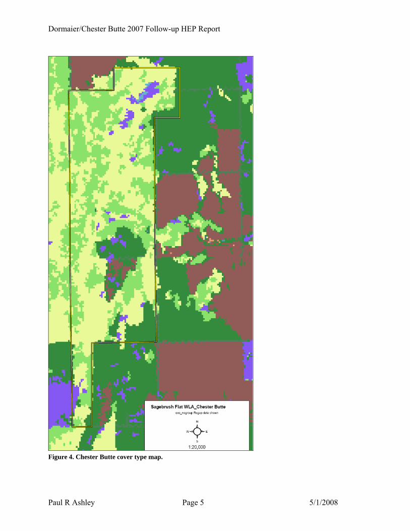
Habitat type classifications shown on Figure 4 were obtained from the 2006 GAP analysis (Ohmann et al. 2006). Cover types in Figure 4 were grouped/generalized as follows for the 2007 follow-up HEP evaluation: dark green and brown = CRP/abandoned agriculture, purple = steppe grassland, and light yellow and light green = shrubsteppe.



Figure 4. Chester Butte cover type map.



Cover Type Descriptions Shrubsteppe (shrub component) is the dominant cover type at the Dormaier and Chester Butte project sites comprising nearly 91% of the combined acreage. In contrast, grasslands covered approximately 9% of the landscape. In either case, vegetation components and structural conditions are nearly identical for both sites. As a result, the following cover type descriptions are applicable to both the Dormaier and Chester Butte properties.

Shrubsteppe The shrubsteppe cover type is defined as xeric uplands with ≥ 5% shrub cover and ≤ 5% tree canopy dominated by native shrubsteppe vegetation and/or invasive species. Shrub species recorded during the 2007 HEP transects included big sagebrush (Artemisia tridentata), three-tip sagebrush (A. tripartite), rigid sagebrush (A. rigida), gray rabbitbrush (Chrysothamnus nauseosa), green rabbitbrush (Chrysothamnus viscidiflorus), currant (Ribes spp.) and gray horsebrush (Tetradymia canescens). The herbaceous layer was comprised of both native and introduced species e.g., bluebunch wheatgrass (Pseudoroegneria spicata), Sandberg bluegrass (Poa secunda), and cheatgrass (Bromus tectorum). An example of the shrubsteppe cover type located on the Dormaier parcel is illustrated in Figure 5.

Figure 5. Dormaier property shrubsteppe cover type example (2007).

Grassland Grassland is defined as “steppe” vegetation dominated by grass and forbs; comprised of both native and non-native species. Percent shrub or tree cover is less than 5%. The grassland cover type includes undisturbed native grasslands, CRP fields, Soil Bank lands, pastures and, in some



cases, abandoned agriculture fields. Typical grass and forbs species included bluebunch wheatgrass, Sandberg bluegrass, fescue (Festuca spp.), cheatgrass, jointed goatgrass (Aegilops cylindrical), Salsify (Tragopogon dubius), and mustards (Brassica spp.) to name a few. Examples of the grassland cover type at Chester Butte are illustrated in Figure 6 and Figure 7. Grassland development on the Dormaier site was initiated in 2007. An example of a new grassland site is shown in Figure 8.

Figure 6. Grassland cover type example at Chester Butte (transect 5).



Figure 7. Grassland cover type example at Chester Butte (transect 14).

Figure 8. Grassland cover type enhancement on the Dormaier site (Transect 3 - April 2007).



Methods

Habitat Evaluation Procedures A follow-up habitat evaluation procedures analysis was conducted on the Dormaier and Chester Butte acquisitions to document changes in baseline habitat suitability/quality. HEP, developed by the U.S. Fish and Wildlife Service (USFWS), is used to quantify the impacts of development, protection, and restoration projects/measures on terrestrial and aquatic habitats by assessing changes, both negative and positive, in habitat quality and quantity (USFWS 1980), (USFWS 1980a). HEP is a habitat based approach to impact assessment that documents change through use of a habitat suitability index (HSI). The HSI value is derived from an evaluation of the ability of key habitat components to provide the life requisites of selected wildlife and fish species. The HSI value is an index to habitat carrying capacity for a specific species or guild of species based on a performance measure (e.g. number of deer per square mile) described in HEP species models. The index ranges from 0.0 to 1.0. A HSI of 0.3 indicates that habitat quality/carrying capacity is marginal while a HSI of 0.7 suggests that habitat quality/carrying capacity is relatively good for a particular species (Table 2). Table 2. Habitat suitability index verbal equivalency table.

Habitat Suitability Index Verbal Equivalent 0.0 < 0.2 Poor 0.2 < 0.4 Marginal 0.4 < 0.6 Fair 0.6 < 0.9 Good 0.9 < 1.0 Optimum

Each increment of change is identical. For example, a change in HSI from 0.1 to 0.2 represents the same magnitude of change as a change from 0.2 to 0.3, and so forth. Habitat variables, suggested mensuration techniques, and mathematical aggregations of assessment results are included in HEP evaluation species models. Habitat units are determined by multiplying the habitat suitability index by the number of acres of habitat (cover type) protected. For example, if the HSI output for a mule deer HEP model is 0.5 and the number of acres of shrubsteppe habitat protected is 100, then the number of HUs is 50 (0.5 HSI x 100 acres = 50 HUs).

HEP Model Selection With exception of the mule deer HEP model, the Regional HEP Team used the same HEP species models in the 2007 follow-up HEP analyses as were used to assess baseline habitat



conditions at the Dormaier site in 1996 and at Chester Butte in 1999. HEP models for the follow-up HEP surveys included mule deer (Ashley and Berger 1999), Sage grouse (Ashley 1996), western meadowlark (Sturnella neglecta) (Schroeder and Sousa 1982), and pygmy rabbit (Ashley 1996). WDFW identified sage grouse and pygmy rabbit as keystone shrubsteppe obligate species (M. Schroeder, pers. comm.) and mule deer an important big game resource. Both pygmy rabbits and sage grouse are protected species in Washington State. Pygmy rabbit replaced western meadowlark as an evaluation species at the Dormaier site. The follow-up HEP species/cover type matrix is shown in Table 3 while abbreviated HEP models are included in Appendix A. Table 3. Dormaier and Chester Butte cover type/species matrix.

HEP Model Project Site Cover Type Western

Meadowlark Sage

Grouse Mule Deer

Pygmy Rabbit Total

Shrubsteppe X X X 3 Dormaier Grassland X X X 3

Shrubsteppe X X X 3 Chester

Butte Grassland X X X 3

HEP Species Model Selection Rationale Species selection rationale described in the Grand Coulee Dam Loss Assessment (Howerton et al. 1986) and other sources including WDFW species management plans and documents are summarized in Table 4. Table 4. HEP model species selection rationale table.

HEP Model Rationale

Mule deer This species represents wildlife dependent upon shrubsteppe and river breaks.

Western meadowlark Represents wildlife species dependent upon grassland and/or shrubsteppe habitats with limited shrub cover.

Sage grouse Represents shrubsteppe obligate species. Pygmy rabbit Represents shrubsteppe obligate species.

Sampling Design and Measurement Protocols

Meta Data Level one meta data follows that suggested by Gotelli and Ellison (2004). Field surveys were conducted by the Columbia Basin Fish and Wildlife Authority’s Regional HEP Team with assistance from WDFW Wildlife Area Assistant Dan Peterson. Regional HEP Team members included Paul Ashley (RHT Coordinator), Mike Cantonese (Team Leader), Anthony Muse, Paul Walker, and Tiffany Baker (contact Paul Ashley @ [email protected], or through CBFWA at: [503] 229-0191).



Funding for the HEP analyses was provided by the Bonneville Power Administration with RHT administrative support provided by CBFWA. Specific measurement techniques and protocols are described in detail in Appendix B. Measurements were recorded in standard U.S. units except for the Robel pole (Robel et al. 1975), which was recorded in metric units.

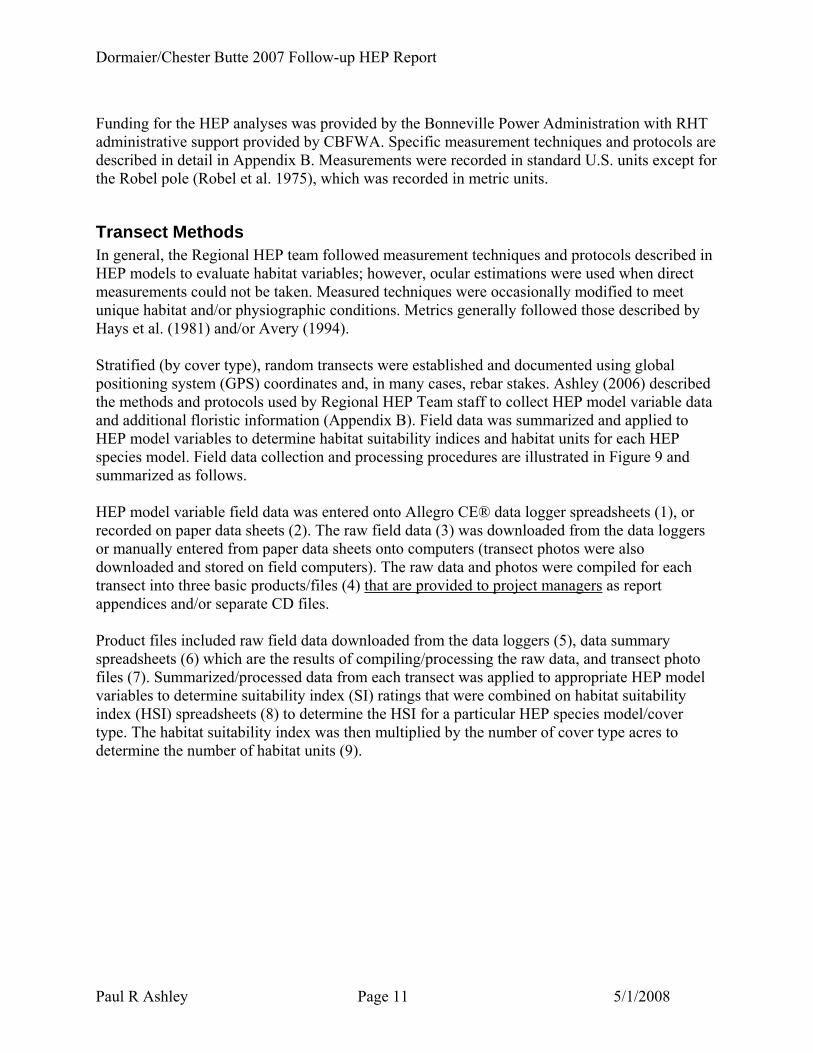
Transect Methods In general, the Regional HEP team followed measurement techniques and protocols described in HEP models to evaluate habitat variables; however, ocular estimations were used when direct measurements could not be taken. Measured techniques were occasionally modified to meet unique habitat and/or physiographic conditions. Metrics generally followed those described by Hays et al. (1981) and/or Avery (1994). Stratified (by cover type), random transects were established and documented using global positioning system (GPS) coordinates and, in many cases, rebar stakes. Ashley (2006) described the methods and protocols used by Regional HEP Team staff to collect HEP model variable data and additional floristic information (Appendix B). Field data was summarized and applied to HEP model variables to determine habitat suitability indices and habitat units for each HEP species model. Field data collection and processing procedures are illustrated in Figure 9 and summarized as follows. HEP model variable field data was entered onto Allegro CE® data logger spreadsheets (1), or recorded on paper data sheets (2). The raw field data (3) was downloaded from the data loggers or manually entered from paper data sheets onto computers (transect photos were also downloaded and stored on field computers). The raw data and photos were compiled for each transect into three basic products/files (4) that are provided to project managers as report appendices and/or separate CD files. Product files included raw field data downloaded from the data loggers (5), data summary spreadsheets (6) which are the results of compiling/processing the raw data, and transect photo files (7). Summarized/processed data from each transect was applied to appropriate HEP model variables to determine suitability index (SI) ratings that were combined on habitat suitability index (HSI) spreadsheets (8) to determine the HSI for a particular HEP species model/cover type. The habitat suitability index was then multiplied by the number of cover type acres to determine the number of habitat units (9).



Figure 9. HEP data collection and processing flow chart.



Transect Locations Using baseline transect maps, photographs, and/or GPS coordinates, the RHT located most baseline transect start point stakes and re-sampled the Dormaier (1966) and Chester Butte (1999) baseline transects. In addition, the Regional HEP Team increased the baseline sample size by adding transects to the 2007 follow-up HEP surveys. The additional 2007 transect initial points (IPs) were established based on stratified random sampling protocols with cover types defining the strata. The number of samples initially allocated per cover type strata were determined based on a proportional allocation strategy (Husch et al. 2003). Specific IP locations were identified by overlaying a 100m x 100m grid over cover types and selecting random numbers to identify “XY” point coordinates (P. Ashley, pers. comm.). The proportional allocation strategy was modified in the field as needed to compensate for the relative homogeneity of a particular cover type, to account for unanticipated access issues and/or physiographic restrictions, and/or to meet temporal considerations. Furthermore, initial points were moved when they did not fall within the cover type(s) of interest, or were in inaccessible areas such as the middle of a pond or cliff area (additional transect information is located in Appendix B). Transect UTM coordinates (NAD 27) for start, turn, and end points were recorded in the field on a Garmin IIIA ® GPS unit. Surveyed transect start points are illustrated in Figure 10 for the Dormaier tract and Figure 11 for Chester Butte. HEP transect UTM coordinates, magnetic azimuths, and lengths are summarized in Table 5.



Figure 10. Dormaier 2007 follow-up HEP transect start points.



Figure 11. Chester Butte 2007 follow-up HEP transect start points.



Table 5. Dormaier and Chester Butte 2007 follow-up HEP transect UTM coordinates, magnetic azimuths, and transect lengths.

GPS Transect Point

E N

Magnetic Azimuth (Degrees)

Length (Feet) Total Length

Dormaier 1 start 11 T 0307226 5283434 226 300 300 end 11 T 0307152 5283389 2 start 11 T 0307072 5283111 270 200 300 turn 11 T 0307003 5283127 225 100 end 11 T 0306984 5283126 3 start 11 T 0306781 5283111 103 300 300 end 11 T 0306860 5283061 4 start 11 T 0307396 5284215 198 300 300 end 11 T 0307313 5284168 5 start 11 T 0306757 5284009 067 300 600 turn 11 T 0306849 5284002 022 300 end 11 T 0306910 5284071

22 start 11 T 0306723 5283372 306 600 600 end 11 T 0306618 5283516

23 start 11 T 0307146 5283585 360 300 300 end 11 T 0307146 5283685 (End coordinates are estimated)

Chester Butte 1 start 11 T 0309876 5285842 305 600 600 end 11 T 0309768 5285996

2 start 11 T 0309691 5286487 360 600 600 end 11 T 0309648 5286304

3 start 11 T 0309641 5286499 172 600 600 end 11 T 0309593 5286325

4 start 11 T 0309921 5287407 189 600 600 end 11 T 0309870 5287218

5 start 11 T 0309717 5287326 169 600 600 end 11 T 0309690 5287140

6 start 11 T 0309501 5287595 269 300 300 end 11 T 0309402 5287623

8 start 11 T 0309716 5288587 300 900 900 end (End coordinates not available)

9 start 11 T 0309099 5288851 230 300 300 end 11 T 0309230 5289463

10 start 11 T 0309230 5289463 203 300 300 end 11 T 0309166 5289388

11 start 11 T 0309323 5286771 282 300 300 end 11 T 0309247 5286811

12 start 11 T 0309131 5286885 169 300 300 end (End coordinates not available)



GPS Transect Point

E N

Magnetic Azimuth (Degrees)

Length (Feet) Total Length

13 start 11 T 0308935 5286268 196 300 300 end 11 T 0308875 5286201

14 start 11 T 0309050 5286236 042 300 300 end 11 T 0309135 5286265

15 start 11 T 0309699 5286322 052 300 300 end 11 T 0309786 5286357

16 start 11 T 0309791 5290992 270 300 300 end 11 T 0309704 5291002

17 start 11 T 0308447 5209387 110 300 300 end 11 T 0308516 5289330

18 start 11 T 0308501 5287819 038 300 300 end 11 T 0308578 5287879

19 start 11 T 0308354 5287337 078 300 300 end 11 T 0308448 5287326

Transect Photo Documentation Transects were photographed with a Canon G1® 3.3 mega pixal digital camera (with and without magnification). Transect photographs are included in Appendix C.

Photo Methods Photo points were established at the start point of each transect to document extant habitat conditions. Digital photographs were recorded from a height of three feet at the beginning of each transect facing the same direction as the transect azimuth. A transect reference board3 was placed at the 15 foot interval while a cover board, divided into 3 inch x 4 inch (8cm x 10cm) rectangles, was set at the 30 foot mark on each transect. Panoramic photographs were also recorded to document dense vegetation, linear/narrow cover types, etc. An example of a photo documentation point is illustrated in Figure 12.

3 Showing transect number, project name, date, GPS reference number



Figure 12. Photo point example.

Results Follow-up habitat evaluation procedures (HEP) analyses were conducted on the Dormaier and Chester Butte wildlife mitigation sites in April 2007 to document current habitat quality/suitability, and when compared to baseline HEP results, determine the number of additional habitat units to credit Bonneville Power Administration (BPA) for providing funds to enhance, and maintain the project sites. The Dormaier follow-up HEP survey generated 482.92 habitat units (HU) or 1.51 HUs per acre for an increase of 34.92 HUs over baseline credits (Table 6). Likewise, 2,949.06 HUs (1.45 HUs/acre) were generated from the Chester Butte follow-up HEP analysis for an increase of 1,511.29 habitat units above baseline survey results (Table 7). In summary, an additional 1,546.21 habitat units (1.46 HUs per acre) were generated by Washington Department of Fish and Wildlife’s (WDFW) passive and active restoration efforts on the Dormaier and Chester Butte parcels. HEP models and habitat suitability mathematical aggregations are included in Appendix A.



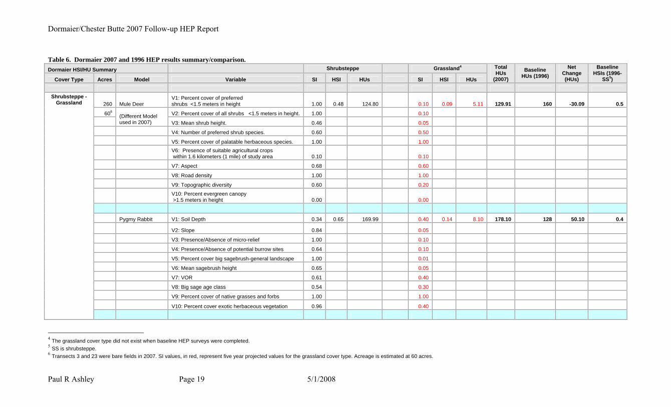
Table 6. Dormaier 2007 and 1996 HEP results summary/comparison. Dormaier HSI/HU Summary Shrubsteppe Grassland4

Cover Type Acres Model Variable SI HSI HUs SI HSI HUs

Total HUs

(2007)

Baseline HUs (1996)

Net Change (HUs)

Baseline HSIs (1996-

SS5)

260 Mule Deer V1: Percent cover of preferred shrubs <1.5 meters in height 1.00 0.48 124.80 0.10 0.09 5.11 129.91 160 -30.09 0.5

606 V2: Percent cover of all shrubs <1.5 meters in height. 1.00 0.10

(Different Model used in 2007) V3: Mean shrub height. 0.46 0.05

V4: Number of preferred shrub species. 0.60 0.50

V5: Percent cover of palatable herbaceous species. 1.00 1.00

V6: Presence of suitable agricultural crops within 1.6 kilometers (1 mile) of study area 0.10 0.10

V7: Aspect 0.68 0.60

V8: Road density 1.00 1.00

V9: Topographic diversity 0.60 0.20

V10: Percent evergreen canopy >1.5 meters in height 0.00 0.00

Pygmy Rabbit V1: Soil Depth 0.34 0.65 169.99 0.40 0.14 8.10 178.10 128 50.10 0.4

V2: Slope 0.84 0.05

V3: Presence/Absence of micro-relief 1.00 0.10

V4: Presence/Absence of potential burrow sites 0.64 0.10

V5: Percent cover big sagebrush-general landscape 1.00 0.01

V6: Mean sagebrush height 0.65 0.05

V7: VOR 0.61 0.40

V8: Big sage age class 0.54 0.30

V9: Percent cover of native grasses and forbs 1.00 1.00

V10: Percent cover exotic herbaceous vegetation 0.96 0.40

Shrubsteppe - Grassland

4 The grassland cover type did not exist when baseline HEP surveys were completed. 5 SS is shrubsteppe. 6 Transects 3 and 23 were bare fields in 2007. SI values, in red, represent five year projected values for the grassland cover type. Acreage is estimated at 60 acres.



Dormaier HSI/HU Summary Shrubsteppe Grassland4

Cover Type Acres Model Variable SI HSI HUs SI HSI HUs

Total HUs

(2007)

Baseline HUs (1996)

Net Change (HUs)

Baseline HSIs (1996-

SS5)

Sage Grouse V1: Percent cover sagebrush 0.90 0.62 162.21 0.10 0.21 12.70 174.92 160 14.92 0.5

V2: Mean sagebrush height 1.00 0.20

V3: Shrub species type 0.50 0.50

V4: Topography 0.84 1.00

V5: Aspect 0.58 0.50

V6: Size of wintering area 1.00 1.00

V7: Percent forbs cover 0.63 1.00

V8: Percent perennial grass cover 1.00 1.00

V9: VOR 0.48 0.30

V10: Percent slope 0.90 1.00

V11: Percent exotic herbaceous cover (weeds) 0.96 0.10

Totals 320 457.01 25.91 482.92 448.00 34.92



Table 7. Chester Butte 2007 and 1998 HEP results summary/comparison. Project: Chester Butte COVER TYPES

HSI/HU Summary Shrubsteppe-2007 Grassland-2007

Cover Type Acres

SI HSI HUs SI HSI HUs

Follow-up HUs (2007)

Baseline HUs

(1999) Net HU Change

Model Variable

Shrubsteppe 2,028 V1: % C.C. Herb. Plants 0.62 0.21 435.28 0.80 0.61 109.41 544.69 351.76 192.93 Grassland 178 V2: % Herb. C.C. Composed of Grass 0.99 1.00 V3: Ave. Ht. of Herb. Canopy 0.60 0.57 V4: Distance to Perch Sites 1.00 0.83

W. Meadowlark

V5: % Shrub Canopy Cover 0.35 1.00

V1: Percent cover of preferred shrubs <1.5 meters in height 0.77 0.54 1,100.80 0.05 0.05 9.40 1,110.20 678.14 432.06

V2: Percent cover of all shrubs <1.5 meters in height. 0.77 0.05 V3: Mean shrub height. 0.51 0.10 V4: Number of preferred shrub species. 0.62 0.33 V5: Percent cover of palatable herbaceous species. 0.91 1.00

V6: Presence of suitable agricultural crops within 1.6 kilometers (1 mile) of study area 0.10 0.10

V7: Aspect 0.65 0.65 V8: Road density 0.95 0.95 V9: Topographic diversity 1.00 1.00

Mule Deer

V10: Percent evergreen canopy >1.5 meters in height 0.00 0.00

V1: Percent cover sagebrush 0.95 0.62 1,260.75 0.12 0.19 33.42 1,294.17 407.87 886.30 V2: Mean sagebrush height 1.00 0.37 V3: Shrub species type 0.50 0.33 V4: Topography 0.75 0.75 V5: Aspect 0.50 0.50

V6: Size of wintering area 1.00 1.00

V7: Percent forbs cover 0.91 0.72

V8: Percent perennial grass cover 1.00 1.00

V9: VOR 0.42 0.45

V10: Percent slope 0.75 0.75

Sage Grouse

V11: Percent exotic herbaceous cover (weeds) 0.73 0.10

Totals 2,206 2,796.83 152.23 2,949.06 1,437.77 1,511.29



Discussion

Dormaier Dense stands of sagebrush (Artemisia spp.) were present on abandoned agricultural lands when the 1996 baseline HEP surveys were conducted (the grassland cover type did not exist in 1996). In 2007, WDFW staff removed the sagebrush converting the abandoned agriculture fields to grassland to increase edge effect and habitat diversity on the site (D. Peterson, pers. comm.). The new grasslands were bare fields during the 2007 HEP surveys as illustrated in Figure 13.

Figure 13. Conversion of abandoned agriculture land to grassland at the Dormaier property in 2007.

Habitat Suitability Since the new grasslands were bare ground in 2007, the Regional HEP Team estimated what grassland habitat suitability and associated habitat units might be for pygmy rabbit, mule deer, and sage grouse in the year 2012. As projected in Table 6, habitat quality is expected to be low for target species for the next five years as grasslands become established. Shrubsteppe habitat suitability indices increased over baseline HSIs for pygmy rabbit and sage grouse due primarily to increased herbaceous cover and relatively low occurrence of exotic vegetation; both of which likely the result of cessation of livestock grazing. On the other hand,



mule deer HEP model HSI decreased slightly (from 0.50 HSI in 1996 to 0.48 HSI in 2007). RHT staff suggests the slight decrease in HSI is an artifact of using a different mule deer HSI model to determine habitat suitability during the 2007 follow-up HEP surveys.

Chester Butte Like the 1999 baseline HEP surveys, Conservation Reserve Program (CRP) grassland, Soil Bank grassland, and vernal wet meadow cover types were combined for the 2007 follow-up HEP surveys to simplify crediting i.e., the same HEP species models were used to evaluate grassland/herbaceous cover types. Similarly, the two acre ephemeral pond was included in shrubsteppe acreage for crediting purposes because of the relatively small area occupied by the palustrine (pond) cover type (this cover type did not meet the minimum size threshold i.e. , 1% of the total area, or five acres combined, therefore, it was considered a shrubsteppe anomaly). A CRP field at Chester Butte surveyed in 1999 (Figure 14) transitioned from herbaceous vegetation to heavy sagebrush cover and was reclassified as shrubsteppe for the 2007 HEP surveys (Transect 1). Furthermore, shrubs were observed in all CRP fields in 2007.



CRP Grasslands(Est. Enhancement acres)

(35)

(15)

Figure 14. Location of CRP fields at Chester Butte. The transition from grassland to shrubsteppe is documented in Figure 15 and Figure 16. Note that the “green” vegetation in Figure 15 is actually Russian thistle [Salsola spp.] i.e., tumbleweed…few shrubs were present in 1999)

CRP in 1999 – Shrubsteppe in 2007



Figure 15. Chester Butte Transect 1 as grassland cover type in 1999.

Figure 16. Chester Butte Transect 1 transitioned to shrubsteppe cover type in 2007. In early 2007, Sagebrush Flat Wildlife Area staff converted a CRP field, comprised primarily of introduced grass species, to a native-like grassland plant community. Habitat conditions photographed at Transect 9 during the 1999 baseline HEP analysis are compared with habitat conditions documented during the 2007 HEP follow-up in Figure 17 and Figure 18 respectively. Photographs for 1999 and 2007 were taken from the same location and azimuth (i.e., from the baseline HEP survey transect start point stake); however, photographs were recorded using different digital cameras and scales.



Figure 17. Transect 9 (CRP) at Chester Butte in 1999. Baseline (1999) and follow-up (2007) shrubsteppe habitat conditions are compared at Transect 8 in Figure 19 and Figure 20 respectively. Note the increase in herbaceous cover.

Figure 18. Transect 9 grass establishement at Chester Butte in 2007.



Figure 19. Shrubsteppe cover type at Transect 8 (1999).

Figure 20. Shrubsteppe cover type at Transect 8 (2007).



Habitat Suitability Follow-up HEP results clearly show that habitat suitability indices improved above baseline HEP results for all target species (Table 7). For example, CRP grassland habitat suitability for western meadowlark increased from 0.02 HSI in 1999 (WDFW 1999) to 0.61 HSI in 2007. Comparing results of the 1999 baseline and 2007 follow-up HEP surveys within the shrubsteppe cover type, the mule deer baseline HSI was 0.33 (WDFW 1999) while the 2007 follow-up mule deer HSI was 0.54. Similarly, sage grouse habitat suitability increased from an averaged 0.17 HSI in 1999 (WDFW 1999) to 0.62 in 2007. Increases in habitat suitability indices and associated habitat units at Chester Butte are largely the result of passive restoration i.e., the removal of livestock. It should be noted, however, that habitat cover type diversity and ecotones appear to be diminishing as shrubs invade and dominate grassland sites.

Acknowledgements I gratefully acknowledge the hard work and effort provided by WDFW Sagebrush Flat Wildlife Area Assistant Manager Dan Peterson and Regional HEP Team members Mikael Cantonese, Tiffany Baker, Tony Muse, and Paul Walker.



References Ashley, P. R. 1996. Pygmy rabbit HSI model (draft). Washington Department of Fish and

Wildlife. Olympia WA. ______. P. R. 1997. Sage grouse HSI model (draft). Washington Department of Fish and

Wildlife. Olympia WA. Ashley, P. R., and M. Berger 1999. Habitat suitability model mule deer (winter). Washington

Department of Fish and Wildlife. Olympia WA. Colville Confederated Tribes. Nespelem, WA.

Ashley, P. R. 2005. White-tailed deer HEP model (draft). Columbia Basin Fish and Wildlife

Authority. Portland, OR. Spokane Tribe of Indians. Wellpinit, WA. _____. 2006. Habitat evaluation procedures standard measurement protocols and techniques

(draft). Columbia Basin Fish and Wildlife Authority (CBFWA). Portland, OR. Avery, T.E., H. E. Burkhart. 1994. Forest measurements. 4th edition. New York, NY: John Wiley

and Sons. Berger, M. T. and D. Kuehn. 1992. Wildlife impact assessment Chief Joseph Dam Project.

Project N0. 88-44. Bonneville Power Administration. Portland, OR. BPA/WDFW. 1996. Memorandum of Agreement between the Washington Department of

Fish and Wildlife and Bonneville Power Administration for the disbursal of wildlife mitigation funds and mitigation crediting. WDFW. Olympia, WA. BPA. Portland, OR.

Gotelli, N. J., A. M. Ellison. 2004. A primer of ecological statistics. Sinauer Associates, Inc.

Sunderland, MA. Hays, R. L., C. Summers, and W. Seitz. 1981. Estimating habitat variables. Western Energy and

land Use Team. Fort Collins, CO: U.S. Fish and Wildlife Service. Howerton, J., J. Creveling, and B. Renfrow. 1986. Wildlife protection, mitigation, and

enhancement planning for Grand Coulee Dam. Olympia, WA: Washington Department of Fish and Wildlife.

Husch, B., T.W. Beers, and J.A. Kershaw, Jr. 2003. Forest mensuration- 4th edition. Hoboken,

NJ: Wiley and Sons, Inc. Ohmann, J. L., M. J. Gregory, and J. S. Fried. 2006. The Pacific Northwest Regional GAP

Analysis Project. Final report on Mapping of forest ecological systems of map zones 8 and 9 with gradient nearest neighbor imputation. Gap Analysis Program-Biological Resources Division, U.S. Geolical Survey. Pacific Northwest Research Station. USDA Forest Service. Corvallis, OR.



Robel, R. J., J. N. Dayton, and A.D. Hulbert. 1975. Relationship between visual obstruction

measurements and weight of grassland vegetation. Journal of Range Management. 23: 295.

Schroeder, R.L., and P.J. Sousa. 1982. Habitat suitability index models: Eastern meadowlark. U.S. Department of the Interior, Fish and Wildlife Service. FWS/OBS-82/10.29.

USFWS. 1980. Habitat as a Basis for Environmental Assessment, Ecological Services Manual

(ESM) 101. Division of Ecological Services, U. S. Fish and Wildlife Service, Washington, DC: Department of the Interior.

______. 1980a. Habitat Evaluation Procedures (HEP), Ecological Services Manual (ESM) 102.

Division of Ecological Services, U.S. Fish and Wildlife Service, Washington, DC: Department of the Interior.

WDFW. 1999. Sagebrush Flat Wildlife Area Work Plan Addendum. Washington Department of

Fish and Wildlife. Olympia, WA.



Appendix A – Abbreviated HEP Models

Mule Deer

V1: Percent palatable shrub cover < 5 ft in height

0

0.2

0.4

0.6

0.8

1

0 5 10 15 20 30 60 100

Percent Cover

Suita

bilit

y In

dex

V2: Percent cover all shrubs < 5 ft in height

00.10.20.30.40.50.60.70.80.9

1

0 5 10 15 20 30 70 100

Percent Canopy Cover

Suita

bilit

y In

dex

V3: Mean shrub height

0

0.2

0.4

0.6

0.8

1

0 30.4 60.8 91.2 121.6 152

Shrub Height (cm)

Suita

bilit

y In

dex



V6: Presence of suitable agricultural crops within 1.6 kilometers (1 mile) of study area Yes: 0.1 No: 0.0

V4: No. of preferred shrub species

0

0.2

0.4

0.6

0.8

1

1 2 3+Number of Preferred Shrub Species

Suita

bilit

y In

dex

V5: Percent cover palatable herbaceous species

00.20.40.60.8

1

0 15 30 40

Percent

Suita

bilit

y In

dex



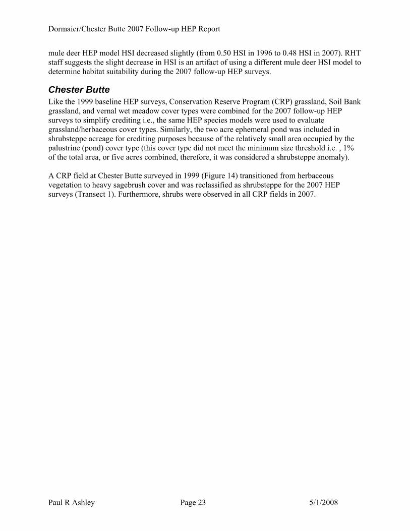
V8: Road density

0

0.2

0.4

0.6

0.8

1

0 1 2 3 4 5 6

Kilometers of Open Road per Square Kilometer

Suita

bilit

y In

dex

V7: Aspect

00.20.40.60.8

1

N NE E SE S SW W NW N

Aspect

Suita

bilit

y In

dex

V9: Topographic diversity

0

0.2

0.4

0.6

0.8

1

A B C D E

DIVERSITY CLASS

Suita

bilit

y In

dex


34

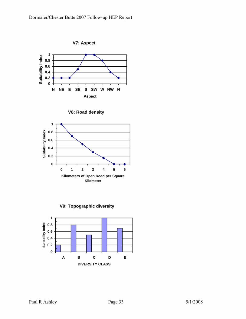
V9 Topographic diversity. A: Level terrain less than 5 percent slope. B: Level terrain broken by drainages. C: Rolling terrain 5 to 25 percent slope. D: Rolling terrain with rims, ridges, and/or drainages. E: Mountainous terrain with slopes greater than 25 percent.

Shrubsteppe HSI = minimum value WFI or WCI WFI = (((V1 (V2 x V3 x V4 x V5) ¼) + V6) x V7)^ .625 x V8 Steps in calculating WFI with a hand calculator:

1. Obtain geometric mean of V2, V3, V4, and V5 2. Multiply product from step one by V1 and add V6 3. Multiply sum obtained in step two by V7 4. Take the 1.66 root (^.6 on your computer)of product from step 3 5. Multiply result from step 4 by V8 to obtain WFI

WCISS = ( V9 x .8 ) + V10 Conifer Forest HSI = Lower Value Between:

WFI = (((V1 (V2 x V3 x V4 x V5) ¼) + V6) x V7)^ .625 x V8

WCIF = 2( V10 ) + V 9 3

V10: Percent evergreen cover > 5 ft in height

0

0.2

0.4

0.6

0.8

1

0 20 40 60 80 100

PERCENT

Suita

bilit

y In

dex


35

Sage Grouse SAGE GROUSE (Cetrocercus urophasianus) HEP MODEL AUTHOR DRAFT 24 Apr 97 Paul R Ashley – Washington Department of Fish and Wildlife Cover Types: Grassland, Shrub-grass, Shrubland (Shrub-steppe) Region: Eastern Washington Winter/Nesting/Brood Rearing HSI SIVI: Percent Crown Cover of Sagebrush

Deep snow limits winter food availability. Sage grouse prefer sagebrush ≥ 25 cm (10 in) hight with ≥ 15% canopy closure (Walkstad and Schladweiler 1974, Shoenberg 1982) and forage in the tallest sagebrush with the greatest canopy cover available (Beck 1977).

SIV2: Mean Height of Sagebrush (cm)

Mean Height of Sagebrush Cover

0

0.2

0.4

0.6

0.8

1

0 20 40 60 70 90 100 120 140

Mean Height of Sagebrush (cm)

HSI

Percent Crown Cover of Sagebrush

0

0.2

0.4

0.6

0.8

1

0 10 20 30 40 50

Percent Sagebrush Cover

HSI


36

Aspect

0

0.2

0.4

0.6

0.8

1

0 45 90 135 170 190 270 315 360

Azimuth (degrees)

HSI

SAGE GROUSE (Cetrocercus urophasianus) HEP MODEL AUTHOR DRAFT SIV3: Species of Shrubs

Shrub Species Ratings: (Braun 1994, Tirhi 1995)

A. No Sagebrush (0.0) B. Big Sagebrush (Artemisia tridentata

tridentata) Three-tipped Sagebrush (A. tripartita) (0.5)

C. Wyoming Big Sagebrush (A. tridentata wyomingensis) Mountain Big Sagebrush (A. t. vaseyana) Stiff Sagebrush (A. rigida) (1.0)

SIV4: Topography Optimum wintering sites are flat or gently sloped (< 15% gradient) with ridges (Jarvis 1974, Beck 1977, Autenrieth 1981, Braun 1994) facing south or west (Beck 1977, Autenrieth 1981, Hupp and Braun 1989). Shroeder (1997) found sage grouse primarily on slopes ≤ 15% during winter and seldom observed sage grouse on slopes ≥ 30% in Eastern Washington. Likewise, Beck (1975) found no sage grouse use on slopes > 30% and most use on slopes < 10%.

SIV5: Aspect (Include local declination)

NOTE: Flat aspects receive an SI = 0.5

Species of Shrubs

0

0.2

0.4

0.6

0.8

1

1.2

A B C

Shrub Species Rating

HSI

Topography

0

0.2

0.4

0.6

0.8

1

0 2.5 5 7.5 10 12.5 15 17.5 20 22.5 25 27.5 30

Percent Slope

HSI


37

Size of wintering area

0

0.2

0.4

0.6

0.8

1

1280 960 640 320

Acres

HS

I

% Forb Crown Cover

0

0.2

0.4

0.6

0.8

1

0 3 5 10 20

% Forb Crown Cover

HS

I

% Perennial Grass Crown Cover

0

0.2

0.4

0.6

0.8

1

0 5 10 15 20

% Per. Grass Crown Cover

HS

I SAGE GROUSE (Cetrocercus urophasianus) HEP MODEL AUTHOR DRAFT SIV6: Size of Wintering Area (acres)

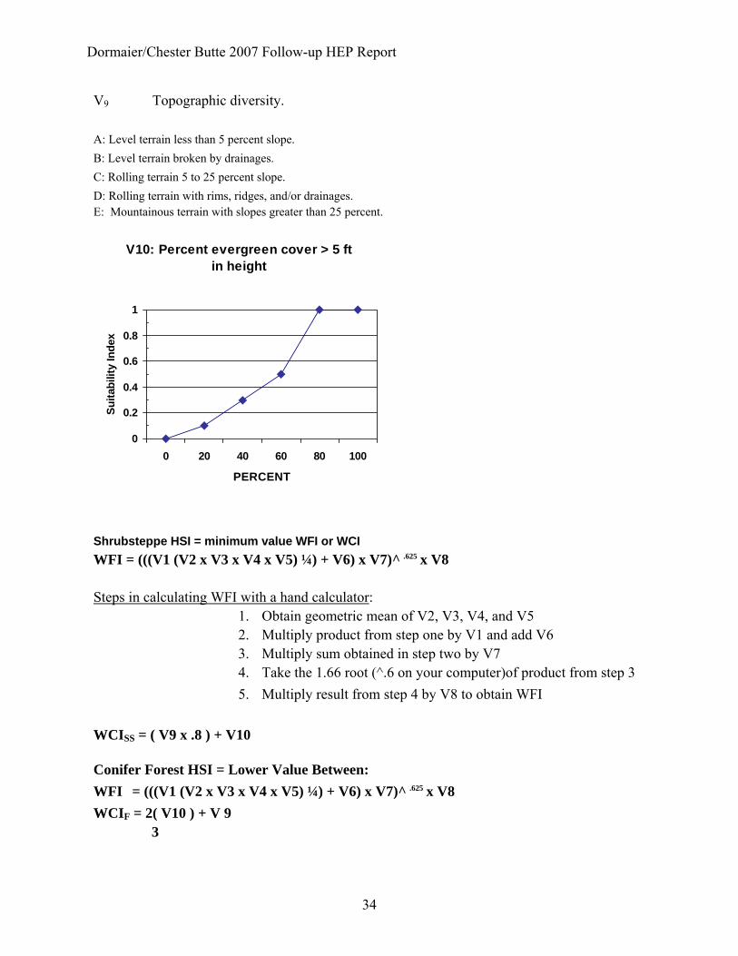
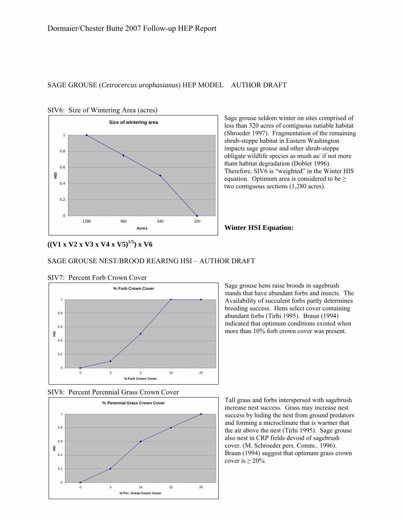
Sage grouse seldom winter on sites comprised of less than 320 acres of contiguous sutiable habitat (Shroeder 1997). Fragmentation of the remaining shrub-steppe habitat in Eastern Washington impacts sage grouse and other shrub-steppe obligate wildlife species as mush as/ if not more thatn habitat degradation (Dobler 1996). Therefore, SIV6 is “weighted” in the Winter HIS equation. Optimum area is considered to be ≥ two contiguous sections (1,280 acres). Winter HSI Equation:

((V1 x V2 x V3 x V4 x V5)1/5) x V6 SAGE GROUSE NEST/BROOD REARING HSI – AUTHOR DRAFT SIV7: Percent Forb Crown Cover

Sage grouse hens raise broods in sagebrush stands that have abundant forbs and insects. The Availability of succulent forbs partly determines breeding success. Hens select cover containing abundant forbs (Tirhi 1995). Braun (1994) indicated that optimum conditions existed when more than 10% forb crown cover was present.

SIV8: Percent Perennial Grass Crown Cover Tall grass and forbs interspersed with sagebrush increase nest success. Grass may increase nest success by hiding the nest from ground predators and forming a microclimate that is warmer that the air above the nest (Tirhi 1995). Sage grouse also nest in CRP fields devoid of sagebrush cover. (M. Schroeder pers. Comm.. 1996). Braun (1994) suggest that optimum grass crown cover is ≥ 20%.


38

VOR - Residual Vegetation

0

0.2

0.4

0.6

0.8

1

0 1 2 3

VOR (dm)

HS

I

Percent Slope

0

0.2

0.4

0.6

0.8

1

0% 5% 10% 15% 20% 25% 30%

Slope

HS

I

% Cover Exotic Weeds

0

0.2

0.4

0.6

0.8

1

0 20 40 60 80 100

% Exotic Crown Cover

HS

I SIV9: Visual Obstruction Reading (VOR) of Residual Vegetation (dm).

Schroeder (1997) suggest that optimum Visual Obstruction Readings (vORs) at nest sites exceed two decimeters (dm). The Robel Pole (Robel 1970) is used to measure the combined cover (VOR) provided by grasses, forbs, and shrubs.

SAGE GROUSE NEST/BROOD REARING HSI – AUTHOR DRAFT SIV10: Slope

Sage grouse prefer to nest on sites with slopes less than 25% gradient (Schroeder 1997).

SIV11: Percent Canopy Cover of Exotic Weeds

Exotic vegetation can significantly degrade shrub-steppe habitat and be difficult to eradicated once established (Dobler pers. comm., 1996). In most instances cheatgrass, Medusa head and other similar invader species replace desirable native grass and forbs. This variable describes nesting/brood rearing habitat quality.


39

Nesting/Brood Rearing HSI Equation: (V7 x V8 x V9)0.333 x (V10 x V11)0.5 Model Equations:

1. Single cover type - Lowest HSI (i.e. Winter HSI or Nesting/Brood Rearing HSI). 2. Multi cover type/landscape – (Winter HSI x Nesting/Brood Rearing HSI) 1/2


40

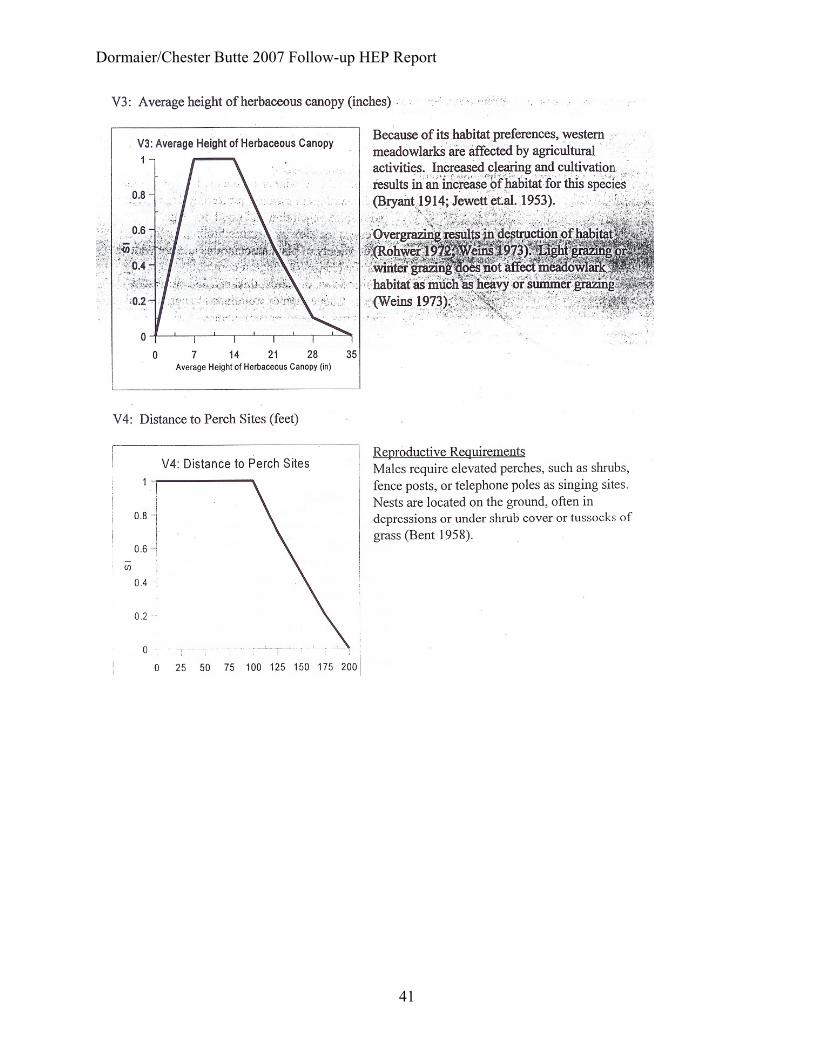
Western Meadowlark


41


42

HSI = (V1 x V2 x V3 x V4)½ x V5


43

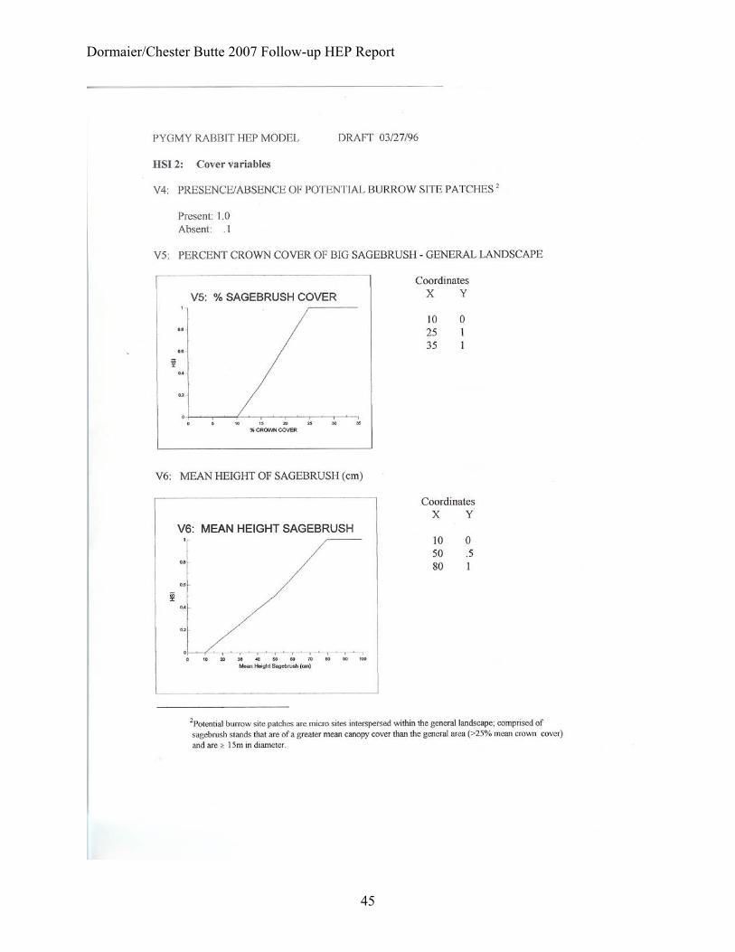
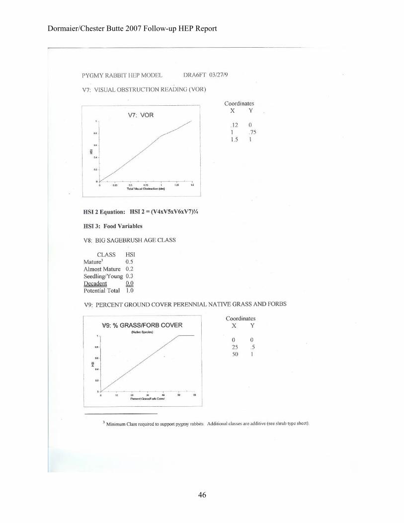
Pygmy Rabbit


44


45


46


47


48

Appendix B – Measurement Protocols

HABITAT EVALUATION PROCEDURES

STANDARD MEASUREMENT PROTOCOLS AND TECHNIQUES (Draft)

Compiled By Paul R Ashley – RHT Coordinator

November 2006


49

HEP Sampling Design and Measurement Protocols Introduction This document was developed to fulfill a request by the Upper Columbia United Tribes (UCUT) and Bonneville Power Administration (BPA) to develop a “stand alone” reference for Habitat Evaluation Procedures (HEP) transect protocols used by the Regional HEP Team (RHT). General and specific protocols are described. General protocols include a brief description of pre HEP survey pilot studies; transect establishment guidelines, and photo documentation parameters. In contrast, specific metrics detail actual habitat variable measurement techniques including diagrams where additional explanation is needed. Specific metrics are identified with an alpha-numeric code. This allows project managers and others to identify specific measurement techniques in report tables without lengthy, redundant explanations. This report is intended to be a “living” document and will be modified as needed. The following standardized protocols and measurement techniques are used by the Regional HEP team to measure habitat variables described in HEP models. General Protocols Pilot Studies Pilot studies are conducted in new habitat types and/or familiar habitat types that are comprised of unique structural conditions/key ecological correlates. Pilot study data is used to estimate the sample size needed for a confidence level ≥ 80% with a 10% tolerable error level (Avery 1994) and to determine the most appropriate sampling unit7 for the habitat variable of interest i.e., a coefficient of variation analysis (BLM 1998). In addition, a power analysis is conducted on pilot study data (and periodically throughout data collection) to ensure that sample sizes are sufficient to identify a minimal detectable change of 20% in the variable of interest with a Type I error rate ≤0.10 and P = 0.9 (BLM 1998, Block et al. 2001). All field data is recorded on data loggers or data sheets and downloaded/transferred to data summary spreadsheets. Transects Transect cover sheets are used to document specific transect information including transect identification, cover type, HEP Team members, global positioning system (GPS) coordinates, and other pertinent information. Transects are established at least 300 feet (100 meters), where possible, from ecotones, roads, and other anthropogenic influences. Transect starting points and azimuths (direction) are randomly selected for each cover type. Start points are selected based on superimposing a UTM grid over cover type maps and identifying specific X/Y coordinates with the aid of a random numbers table, or computer generated random number generator/point locater program. Transect start, turn, and end points are marked with 14-inch (36 centimeter) 0.25 inch (0.6 centimeter) diameter rebar stakes8 painted fluorescent orange or red. GPS positions (UTM coordinates-NAD 27) are recorded at start, turn, and end points. If cover types change or transect length is greater than 300 feet, another transect azimuth is randomly selected, or the original azimuth is varied by 45 degrees (direction [left or right] is determined by the flip of a coin where 7 Includes micro-plot grid size and shape etc. 8 Marking transect points with rebar stakes is at the discretion of the project proponent. Therefore, not all transects are marked in this manner.


50

more than one choice is possible). Compass azimuths (headings) are magnetic bearings i.e., not corrected for local declination. Transects are divided into 100 foot (30 meter) sample units for statistical purposes. Photo Points Photo points are established at the start point of each transect. Pictures are recorded from a height of three feet at the beginning of each transect while facing in the direction of the transect azimuth. A transect reference board (includes transect number, project name, date, GPS reference number) is placed at the 15 foot interval while a cover board is placed at the 30 foot mark on each transect. Occasionally, panoramic photographs are also needed e.g., dense vegetation, linear/narrow cover types. Habitat conditions are photographed with a Canon G1® 3.3 mega pixal digital camera (with and without magnification). Specific Metrics Metrics generally follow those described by Hays et al. (1981) and/or Avery (1994) unless otherwise noted. Some metrics have been modified due to extreme field conditions and/or to better meet Regional HEP Team needs. Herbaceous Measurements Percent Cover

1. Herbaceous percent cover measurements are recorded at 20 or 25-foot intervals on the right side of the transect tape (the right side is determined by standing at 0 feet and facing the line of travel/transect azimuth). RHT members walk on the left side of the transect line to reduce sample disturbance. A square 0.1m2 micro-plot grid is used in grasslands to estimate percent cover of herbaceous vegetation while a rectangular 0.5m2 grid is generally used in shrublands (the 0.5m2 grid may also be used in grasslands if desired). The near right hand corner of the grid is placed at the sampling interval (rectangle grids are placed with the long axis perpendicular to the tape, and the lower right corner on the sampling interval). An example of micro-plot grid placement is shown in Figure 1. Approximately 20% of the micro plot is covered by vegetation in the example. Grid samples are considered independent samples for statistical purposes.

1A: 0.1m2 micro-plot grid/20’ interval 1B: 0.1m2 micro-plot grid/25’ interval 1C: 0.5m2 micro-plot grid/20’ interval 1D: 0.5m2 micro-plot grid/25’ interval


51

Figure 1. Micro-plot grid placement and percent cover example. Height

2. Herbaceous height is measured with a measuring rod placed within the grid frame (scale = 10ths/ft.). Three evenly spaced measurements are recorded and averaged for each sample. Only leaf material is measured (leaves provide the greatest amount of cover). “Leaf material” may include residual cover and/or new growth predicated on HEP model variable requirements. Grass inflorescence is not included in height measurements. 2A. Four measurements, one from each corner of the micro plot grid, are recorded and averaged for each sample. Only leaf material is measured (leaves provide the greatest amount of cover). Grass inflorescence is not included in height measurements. 2B. A measuring rod is held vertical at the interval point: the highest vegetation to cross the measuring rod at that point is measured to the nearest tenth of a foot. 2B-1: 10’ interval 2B-2: 20’ interval 2B-3: 25’ interval

Visual Obstruction Readings (VOR)

3. A Robel pole (Robel 1975) is used to document vertical and/or horizontal cover for herbaceous vegetation i.e., visual obstruction readings (VOR). Measurements are recorded at 20, 25, or 50-foot intervals. Intervals are determined by the length of each transect, i.e., a minimum of 12 measurements are required for each transect, or cover type heterogeneity (structurally diverse cover types generally require larger sample sizes). The Robel pole (Robel 1975) is placed on the transect line at the appropriate interval. Four observations are taken from a distance of four meters from the Robel pole and averaged to obtain a single visual obstruction reading or VOR. Observers sight over a one

Transect Line/Direction

25’ Mark

0.10m2 Micro-Plot Grid

Micro-Plot Placement


52

meter pole and record how much of the Robel pole is totally obscured from the ground up (Figure 2). Measurements are reported in 0.25 decimeter increments. Two measurements are taken on the transect line on opposite sides of the Robel pole; two identical measurements are taken from the same point perpendicular to the transect line for a total of four “readings” (Figure 3). Sample size is determined to be adequate when the “running mean” varies ≤ 10% of the mean. VOR samples are considered independent for statistical purposes. 3A: 20’ interval 3B: 25’ interval 3C: 50’ interval

Figure 2. Visual obstruction reading diagram.

Robel Pole

Sighting Pole (1 meter)

4 meter line

2.54 cm x 1 dm

Observation line

(Not to scale)


53

Figure 3. Robel pole “readings” layout diagram. Shrub Measurements Percent Cover

4. Line intercept or point intercept (USFWS 1981) is used to determine shrub cover. Line intercept is generally used when shrub cover is estimated at < 5% (the most accurate results are obtained using the line intercept method). In contrast, the point intercept method is used if shrub cover is estimated at > 5%.

4A: Line intercept is used to measure the amount of cover that intercepts the transect line as illustrated by the red lines shown in Figure 4. Measurements are in 10ths of feet. Gaps in vegetation less than four tenths of a foot (5 inches) are ignored. The amount covered by shrubs is added to determine shrub intercept for each transect. For example, if 7.5 feet of a 100-foot long transect is covered by shrubs, percent cover is 7.5%. Shrub cover is recorded by species. Where shrubs overlap, shrub intercept is recorded for the tallest shrub and noted for the lower shrub(s).

90º Transect Line

Robel Pole

Sighting Pole Locations (4 meters from Robel pole)

Sighting Pole Locations (4 meters from Robel pole)

Perpendicular Observations

(“Birds eye” View)


54

Figure 4. Line intercept method example.

4B: Point intercept is used when shrub canopy cover is estimated at ≥5%. Shrub cover is determined by recording the number of “hits” at specific intervals along a transect line. To be counted as a “hit”, a portion of the shrub must cross the transect tape’s interval number line e.g., 2’, 4’, 6’…. nth. If a portion of the shrub does not break the vertical plane at the interval number line, it is reported as a miss (Figure 5). Either a “hit” or “miss” is recorded on data loggers and/or paper data sheets for each designated interval.

Figure 5. Point intercept method example showing “hits” and “misses” at two foot intervals.

0 ft.

100 ft.

Shrubs

2’ 4’ 6’

Transect Tape

“Hit”

“Miss”

“Hit”


55

From 5% to 20% cover, point data is collected at two-foot intervals (50 possible “hits” per 100 ft. sample unit). If shrub cover is estimated at >20%, shrub point data is collected at five foot intervals (20 possible “hits” per 100 ft. sample unit). On rare occasions, ten-foot intervals may be used when shrub cover exceeds 50% (10 possible “hits” per 100 ft. sample unit). The ten-foot interval is generally applied to shrub monocultures, or areas with few shrub species that exhibit relatively equal shrub distribution/density. Shrub “hits” are recorded by species. Where shrubs overlap, shrub intercept is recorded for the tallest shrub and noted for the lower shrub(s). 4B-1: 2’ interval 4B-2: 5’ interval 4B-3: 10’ interval 4C: Modified point method is used when shrub cover is impenetrable or otherwise inaccessible. A baseline transect is established along the shrub edge. A six-foot measuring rod is then inserted into the shrub cover at right angles to the baseline tape at appropriate intervals. Recorders estimate shrub “hits”, species information, and height data where the end of the six-foot measuring rod intercepts the shrub cover (Figure 6). As with point intercept, intervals may very. Shrubs are identified by species.

4C-1: 2’ interval 4C-2: 5’ interval 4C-3: 10’ interval

Figure 6. Modified point intercept layout example.

4D: Complex shrub intercept is used to determine percent shrub cover in multi strata shrub communities. This method is generally associated with point intercept methods

Shrubs

Transect line

6’ measuring rod Measuring points


56

whereas overlapping shrubs are identified for each stratum. Percent cover is determined for each of four possible strata as well as total percent shrub cover and overlapping percent cover. The complex shrub intercept method is identified by adding the suffix “4D” after the appropriate line or point intercept method. For example, “4B-1-4D designates that complex shrub point intercept measurements were taken at two foot intervals. Similarly, 4C-2-4D designates that modified point intercept at five foot intervals was used to determine percent shrub cover for strata in a complex shrub community.

Shrub Height

5. Shrubs are defined as woody vegetation including trees <16 feet in height unless otherwise defined in HEP models. The Regional HEP Team assumes that trees <16 feet tall function ecologically more like shrubs than trees.

Figure 7. Line intercept shrub height measurement example.

Shrub height is measured in 10ths of feet at the highest point for each uninterrupted line intercept segment as depicted in Figure 7, or the highest point that crosses each point intercept interval mark on the transect tape (Figure 8). In structurally complex (overlapping) shrub communities, height is measured for each stratum (maximum of four) as illustrated in Figure 9. It is assumed that shrub height measurements correspond to the method used to determine percent shrub cover. For example, if percent shrub cover is determined using the line intercept method (Figure 4), then it is assumed that shrub height will be obtained as illustrated in Figure 7.

Line Intercept segment

Transect Line

Measure Height Here

Horizontal View

Shrub(s)


57

Figure 8. Point intercept shrub height example.

Figure 9. Complex shrub community shrub height measurement example.

Tree Measurements Percent Canopy Cover

5 feet 10 feet 15 feet 20 feet

Point Intercept Intervals

Shrub Height Measurements

Transect Line

Stratum 1

Stratum 2

Stratum 3


58

6. Tree canopy cover measurements are recorded at five or ten foot intervals with a densitometer (point intercept). Measurement intervals are determined by visually estimating tree canopy closure prior to initiating the survey. If estimated canopy closure is < 20% and estimated transect length ≤ 900 feet, measurements are recorded at five-foot intervals; if estimated canopy closure is > 20% and estimated transect length is ≥ 600 feet, ten-foot intervals are used. The size of the sample area strongly influences transect length. In small areas, data from several short (300 foot) transects may be “pooled” in order to determine percent tree canopy cover. As with shrubs, sampled trees are identified by species and the sampling unit is a 100 foot segment of the transect. 6A: 5’ interval 6B: 10’ interval Height 7. Tree height is determined generally using a clinometer. In open areas, an electronic height measurement instrument may be used. Measurements are taken at the beginning and end of each transect and at 100 foot intervals. Additional samples may be taken if needed. HEP model variable requirements determine the extent of tree height measurements e.g., multi-canopy, overstory, etc. Basal Area

8. Tree basal area data is collected at 100-foot intervals using a “factor 10” prism. Each 100-foot interval basal area observation (all tree “hits” at each 100-foot point) is considered an independent sample.

Snag DBH

9. Snag data is collected on belt transects. RHT members collect snag data in conjunction with tree canopy closure measurements using the same baseline transect. The diameter breast height (DBH) of all snags present within tenth-acre belt transects paralleling the baseline transect is measured. Either the actual DBH is recorded, or snag data is reported by class e.g., 5 snags <4” DBH, 2 snags >20” DBH etc. Belt transects are 44 feet wide by 100 feet long i.e., 22 feet on each side of the baseline transect. Belt transect layout is depicted in Figure 10. As with shrubs and trees, the sampling unit is each 100-foot segment.


59

Figure 10. Belt transect layout diagram. Sample Size Determination

The process for determining sample size (transect length) varies based on the variable measured. Shrub and tree cover and grid sample sizes are estimated as follows:

The amount of cover within each 100 foot sample unit is divided by sample unit length to obtain percent shrub/tree cover per sample unit (e.g. 10 feet of cover/100 feet = 10% shrub cover). The standard deviation for each transect is calculated for percent cover data from transect sample units. Sample size (transect length) is then determined through use of the following equation (Avery 1994):

n = t2s2

E2

Where: t = t value at the 95 percent (0.05) confidence interval for the appropriate degrees of freedom (df); s = standard deviation; and E = desired level of precision, or bounds (± 10 percent). Confidence intervals may vary from 80 percent (0.20) to 95 percent (0.05) depending on habitat variable heterogeneity and project management needs. The same method is used to determine sample size for micro plot samples based on total percent cover for herbaceous species.

Transect

22 feet

22 feet

100’ Sample Unit 100’ Sample Unit 100’ Sample Unit

10th Acre


60

References Avery, T.E., H. E. Burkhart. 1994. Forest measurements. 4th edition. John Wiley and Sons. New

York, NY. BLM. 1998. Measuring and monitoring plant populations. BLM Technical Reference 1730-1.

BLM National Business Center. Denver, CO. 477 p. Block, W.M., W.L. Kendall, M.L. Morrison, and M. Dale Strickland. 2001. Wildlife study

design. Springer Press. New York, NY. 210 p. Hays, R. L., C. Summers, and W. Seitz. 1981. Estimating habitat variables. Western Energy and

land Use Team. Fort Collins, CO: U.S. Fish and Wildlife Service. Robel, R.J., J. N. Dayton, A.D. Hulbert. 1975. Relationship between visual obstruction

measurements and weight of grassland vegetation. Journal of Range Management. 23: 295.


61

Appendix C – Transect Photographs

Dormaier

Transect 1 Photograph not available

Transect 2


62

Transect 3

Transect 4


63

Transect 5

Transect 22


64

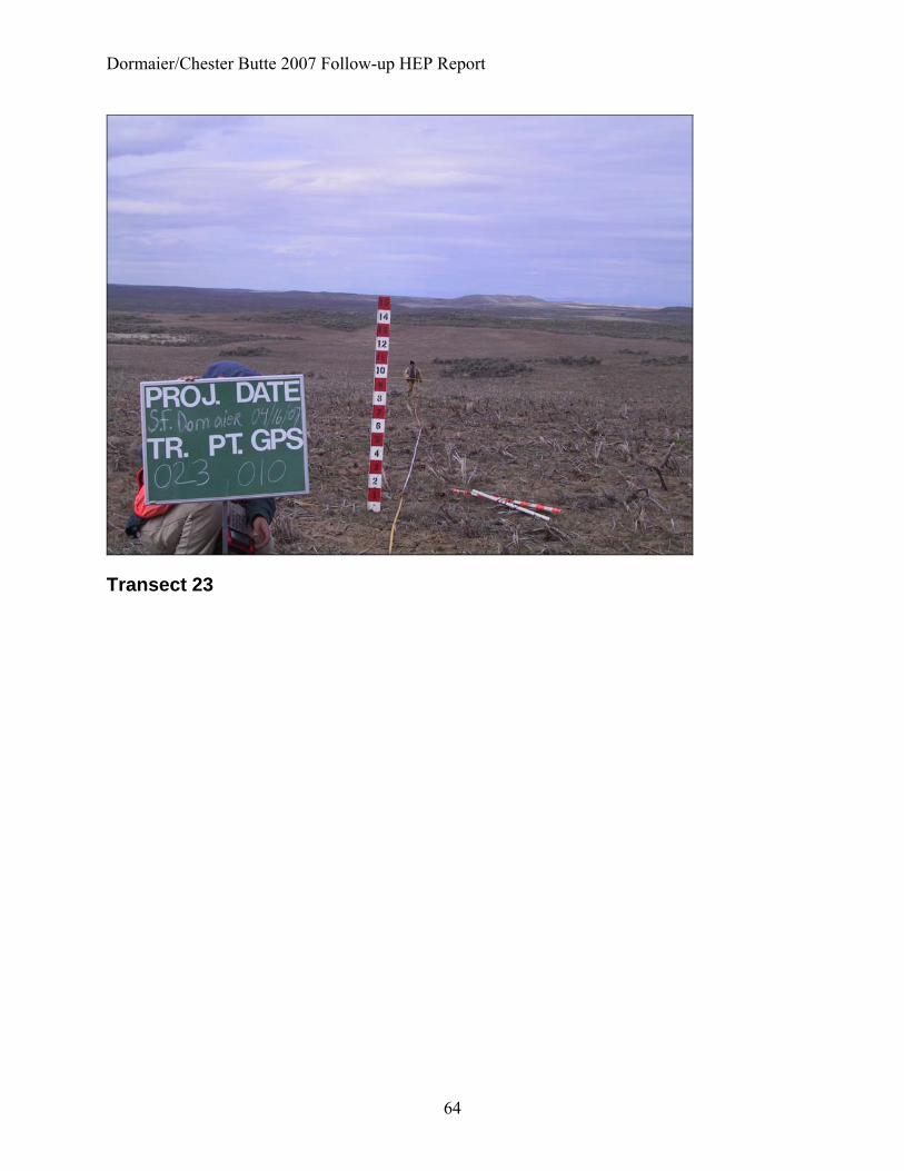
Transect 23


65

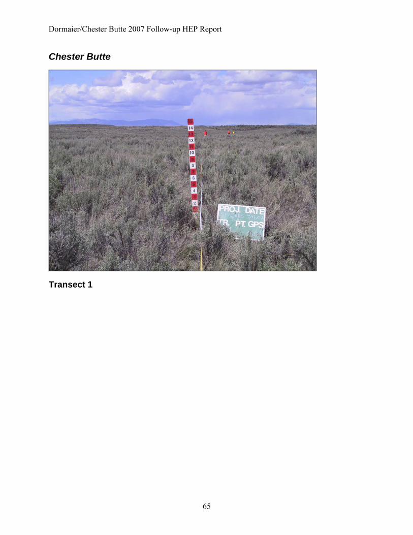
Chester Butte

Transect 1


66

Transect 2

Transect 3


67

Transect 4

Transect 5


68

Transect 6

Transect 8


69

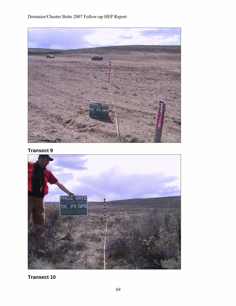
Transect 9

Transect 10


70

Transect 11

Transect 12


71

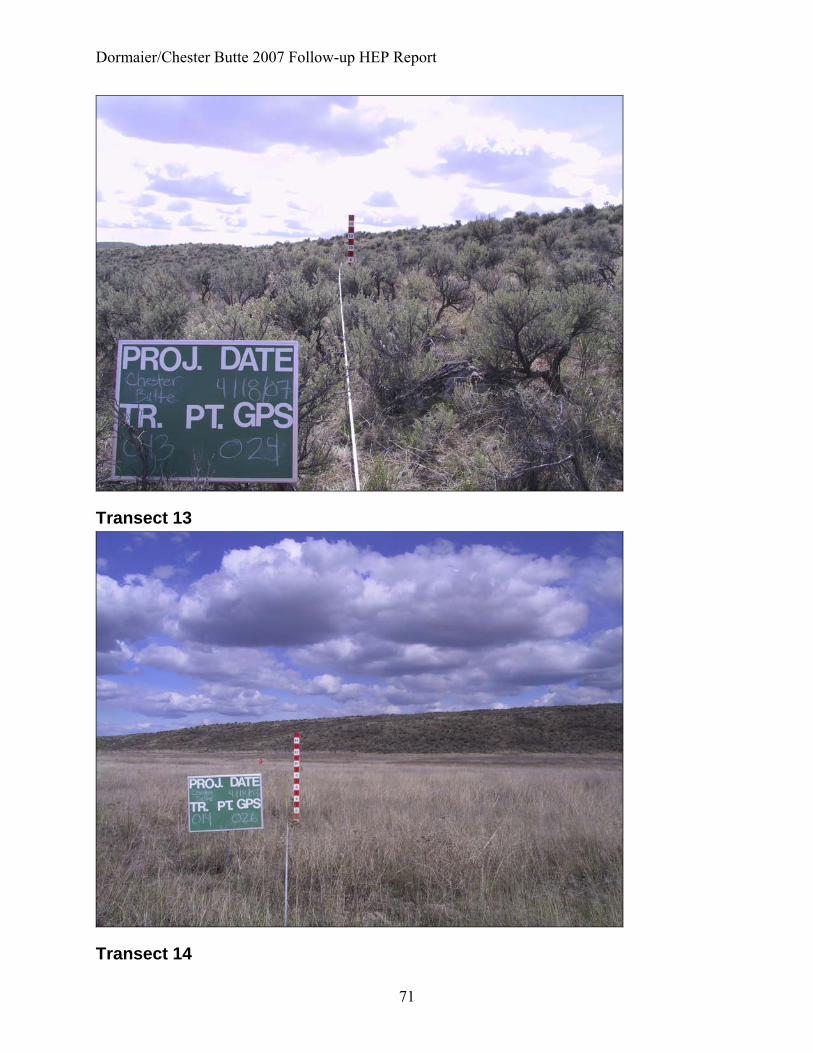
Transect 13

Transect 14


72

Transect 15

Transect 16


73

Transect 17

Transect 18


74

Transect 19

dormaier chester butte 2007 - unt digital library/67531/metadc901712/...dormaier and chester butte...

Documents