don’t optimize yet! - forside - det digitale projektbibliotek,...
TRANSCRIPT
Don’t Optimize Yet!On an approach for making early performance
evaluation usable to Software Engineering
Group E4-114 SupervisorRené Hansen Bent ThomsenDennis Micheelsen

The Faculty of Engineering and ScienceUniversity of Aalborg
Department of Computer Science
TITLE:Don’t Optimize Yet!
SUBTITLE:On an approach for making earlyperformance evaluation usableto Software Engineering
SEMESTER PERIOD:DAT6,1st February 05 - 15th June 05
PROJECT GROUP:E4-114René Hansen,[email protected]
Dennis Micheelsen,[email protected]
SUPERVISOR:Bent Thomsen,[email protected]
NO. COPIES: 6
NO. PAGES: 91
Abstract:
There are three rules to performance opti-mizations: Don’t optimize yet!, Don’t opti-mize yet!, Don’t optimize yet! Tradition-ally, the popular notion towards performancehas been to ignore it until it could no longerbe ignored. However, many companies havefaced the consequence of this approach, find-ing that some performance problems are im-possible to solve through code optimizationalone. A discipline called Software Per-formance Engineering(SPE) tries to alleviateperformance problems before they arise bymodelling performance already at the designphase. However, SPE has never caught onin the mainstream Software Engineering prac-tices - mainly because it relies on specializedperformance staff. In this thesis we propose anapproach making early performance consider-ations more amenable to Software Engineer-ing. We have created a J2ME test applicationthat derives performance characteristics of thetarget environment. The test application canbe used to supply input estimates that wouldotherwise need to be supplied by a SPE spe-cialist. The input estimates from the test appli-cation are used to annotate activity diagramsaccording to the UMLTM Profile for Schedula-bility, Performance, and Time which results inperformance predictions of the system underdevelopment. We have investigated the valid-ity of our approach by applying it to a test case,a J2ME application.


Preface
This thesis is written at the Department of Computer Science at the faculty of Engi-neering and Science. The thesis is written by group E4-114 in the field of Databaseand Programming Technologies. We wish to thank our supervisor Bent Thomsenfor his input and many inspiring sessions throughout the work on this thesis.
Aalborg, June, 2005
Dennis Micheelsen René Hansen

Contents
List of Tables ii
List of Figures iv
List of Listings 1
1 Introduction 3
I Related Work 9
2 Software Performance Engineering 11
2.1 Execution Graphs . . . . . . . . . . . . . . . . . . . . . . . . . .15
2.2 The System Execution Model . . . . . . . . . . . . . . . . . . . .18
2.3 Other approaches . . . . . . . . . . . . . . . . . . . . . . . . . .23
3 Problems and proposed solutions 27
3.1 Problems with SPE . . . . . . . . . . . . . . . . . . . . . . . . .27
3.2 Proposed solutions . . . . . . . . . . . . . . . . . . . . . . . . .32
4 UML TM Profile for Schedulability, Performance and Time 35
4.1 Performance analysis of a UML model . . . . . . . . . . . . . . .37
4.2 Concepts and techniques . . . . . . . . . . . . . . . . . . . . . .38
CONTENTS i
II Our Approach 47
5 Describing our approach 49
5.1 The Record Management System . . . . . . . . . . . . . . . . . .49
5.2 Networking . . . . . . . . . . . . . . . . . . . . . . . . . . . . . 50
5.3 Obtaining input estimates . . . . . . . . . . . . . . . . . . . . . .50
5.4 Using the results . . . . . . . . . . . . . . . . . . . . . . . . . .52
6 Applying our approach 55
6.1 A description of the test case . . . . . . . . . . . . . . . . . . . .55
6.2 Scenarios . . . . . . . . . . . . . . . . . . . . . . . . . . . . . .58
7 Evaluating our approach 65
7.1 Evaluating the RMS results . . . . . . . . . . . . . . . . . . . . .66
7.2 Conlusion on the RMS test results . . . . . . . . . . . . . . . . .72
7.3 Evaluating the network results . . . . . . . . . . . . . . . . . . .73
7.4 Conclusion on the network results . . . . . . . . . . . . . . . . .75
7.5 Overall evaluation of our approach . . . . . . . . . . . . . . . . .75
III Conclusion and future work 79
8 Conclusion 81
8.1 Shortcomings and future work . . . . . . . . . . . . . . . . . . .84
8.2 Summary . . . . . . . . . . . . . . . . . . . . . . . . . . . . . .85
Bibliography 87
List of Tables
5.1 Size of Java primitives . . . . . . . . . . . . . . . . . . . . . . .51
7.1 Results of RMS operations on the logistics application . . . . . .67
7.2 The results returned from the test application emulating the work-load of the logistics application . . . . . . . . . . . . . . . . . . .67
7.3 Results of operations relevant for performing writes obtained fromthe test application . . . . . . . . . . . . . . . . . . . . . . . . .68
7.4 The total write time computed for the avg., max., and 95th mea-sures as well as the total time measured . . . . . . . . . . . . . .69
7.5 The average, minimum, and maximum times for writing on thelogistics application . . . . . . . . . . . . . . . . . . . . . . . . .69
7.6 The percent-wise deviation between the estimates of the test appli-cation and the actual results of the logistics application for writeoperations. . . . . . . . . . . . . . . . . . . . . . . . . . . . . . .69
7.7 Results of operations relevant for performing reads obtained fromthe test application . . . . . . . . . . . . . . . . . . . . . . . . .70
7.8 The total read time computed for the avg., max., and 95th measuresas well as the total read time measured . . . . . . . . . . . . . . .71
7.9 The average, minimum, and maximum times for reading on thelogistics application . . . . . . . . . . . . . . . . . . . . . . . . .71
7.10 The percent-wise deviation between the estimates of the test ap-plication and the actual results of the logistics application for readoperations . . . . . . . . . . . . . . . . . . . . . . . . . . . . . .71
7.11 Results of delete operations obtained from the test application . .72
LIST OF TABLES iii
7.12 The average, minimum, and maximum times for deleting a recordstore on the logistics application . . . . . . . . . . . . . . . . . .72
7.13 The percent-wise deviation between the estimates of the test appli-cation and the actual results of the logistics application for deleteoperations . . . . . . . . . . . . . . . . . . . . . . . . . . . . . .72
7.14 Results of Networking operations in the logistics application . . .73
7.15 Results of Networking operations in the test application . . . . . .74
7.16 Relevant results of Networking operations in the logistics application74
7.17 Relevant results of Networking operations in the test application .74
7.18 The percent-wise deviation between the estimates of the test appli-cation and the actual results of the logistics application for fetchingoperations . . . . . . . . . . . . . . . . . . . . . . . . . . . . . .74
7.19 Relevant results of Networking operations in the logistics application74
7.20 Relevant results of Networking operations in the test application .75
7.21 The percent-wise deviation between the estimates of the test appli-cation and the actual results of the logistics application for the sendoperation . . . . . . . . . . . . . . . . . . . . . . . . . . . . . . 75

List of Figures
2.1 The SPE modelling process [41] . . . . . . . . . . . . . . . . . .14
2.2 Basic execution graph nodes . . . . . . . . . . . . . . . . . . . .16
2.3 Sequence structure . . . . . . . . . . . . . . . . . . . . . . . . .17
2.4 Loop structure . . . . . . . . . . . . . . . . . . . . . . . . . . . .18
2.5 Case structure . . . . . . . . . . . . . . . . . . . . . . . . . . . .18
2.6 Queue-server representation of a resource [41] . . . . . . . . . . .19
2.7 Hypothetical execution profile . . . . . . . . . . . . . . . . . . .20
4.1 The UML profile for Schedulability, Performance, and Time. Theperformance component is indicated by the solid line. . . . . . . .36
4.2 Abstract view of the model processing process [13] . . . . . . . .38
4.3 The Performance analysis domain model [13] . . . . . . . . . . .40
6.1 Test application architecure . . . . . . . . . . . . . . . . . . . . .56
6.2 The overall activity diagram . . . . . . . . . . . . . . . . . . . .57
6.3 Get Route w/time activity diagram . . . . . . . . . . . . . . . . .59
6.4 Save persistent w/time activity diagram . . . . . . . . . . . . . .60
6.5 Read persistent w/time activity diagram . . . . . . . . . . . . . .61
6.6 Abruption w/with activity diagram . . . . . . . . . . . . . . . . . 62
6.7 Finish route w/ time activity diagram . . . . . . . . . . . . . . . .63

LIST OF FIGURES v
7.1 The input screen for the RMS test on the test application . . . . .66
7.2 The class diagram for the route . . . . . . . . . . . . . . . . . . .67
Listings
1.1 Calculating a row sum . . . . . . . . . . . . . . . . . . . . . . . 4
1.2 Calculating a row sum (optimized) . . . . . . . . . . . . . . . . . 4
5.1 Example customer class . . . . . . . . . . . . . . . . . . . . . . .51

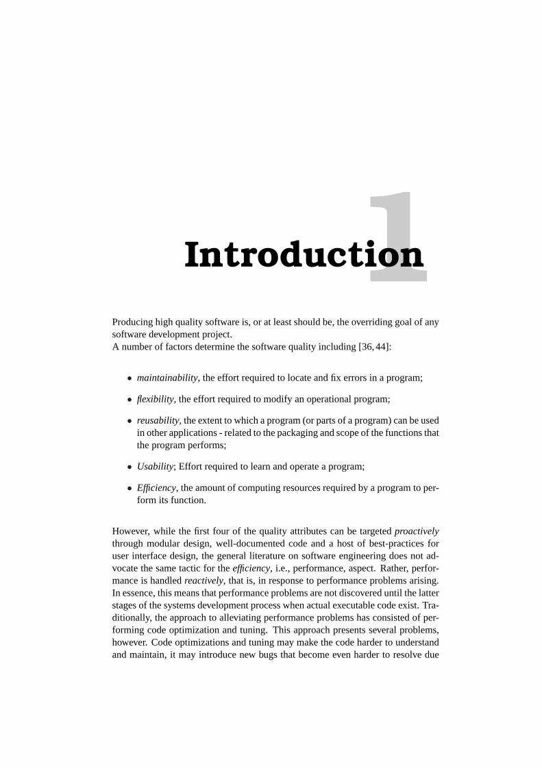
1Introduction
Producing high quality software is, or at least should be, the overriding goal of anysoftware development project.A number of factors determine the software quality including [36,44]:
• maintainability, the effort required to locate and fix errors in a program;
• flexibility, the effort required to modify an operational program;
• reusability, the extent to which a program (or parts of a program) can be usedin other applications - related to the packaging and scope of the functions thatthe program performs;
• Usability; Effort required to learn and operate a program;
• Efficiency, the amount of computing resources required by a program to per-form its function.
However, while the first four of the quality attributes can be targetedproactivelythrough modular design, well-documented code and a host of best-practices foruser interface design, the general literature on software engineering does not ad-vocate the same tactic for theefficiency, i.e., performance, aspect. Rather, perfor-mance is handledreactively, that is, in response to performance problems arising.In essence, this means that performance problems are not discovered until the latterstages of the systems development process when actual executable code exist. Tra-ditionally, the approach to alleviating performance problems has consisted of per-forming code optimization and tuning. This approach presents several problems,however. Code optimizations and tuning may make the code harder to understandand maintain, it may introduce new bugs that become even harder to resolve due
4 Introduction
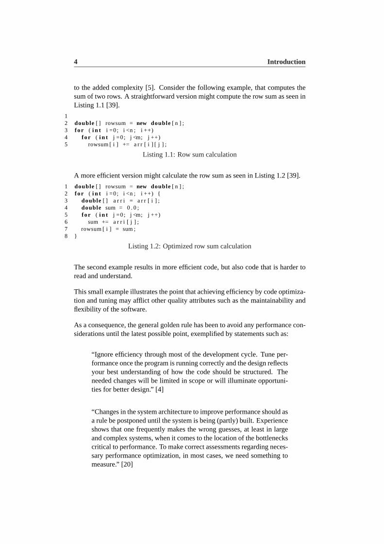
to the added complexity [5]. Consider the following example, that computes thesum of two rows. A straightforward version might compute the row sum as seen inListing 1.1 [39].
12 double [ ] rowsum = new double[ n ] ;3 f o r ( i n t i =0 ; i <n ; i ++)4 f o r ( i n t j =0 ; j <m; j ++)5 rowsum [ i ] += a r r [ i ] [ j ] ;
Listing 1.1: Row sum calculation
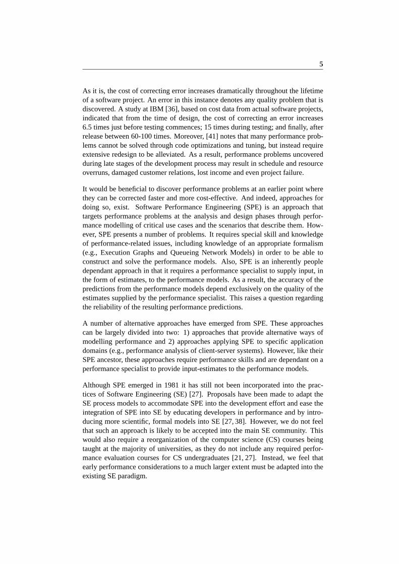
A more efficient version might calculate the row sum as seen in Listing 1.2 [39].
1 double [ ] rowsum = new double[ n ] ;2 f o r ( i n t i =0 ; i <n ; i ++) {3 double [ ] a r r i = a r r [ i ] ;4 double sum = 0 . 0 ;5 f o r ( i n t j =0 ; j <m; j ++)6 sum += a r r i [ j ] ;7 rowsum [ i ] = sum ;8 }
Listing 1.2: Optimized row sum calculation
The second example results in more efficient code, but also code that is harder toread and understand.
This small example illustrates the point that achieving efficiency by code optimiza-tion and tuning may afflict other quality attributes such as the maintainability andflexibility of the software.
As a consequence, the general golden rule has been to avoid any performance con-siderations until the latest possible point, exemplified by statements such as:
“Ignore efficiency through most of the development cycle. Tune per-formance once the program is running correctly and the design reflectsyour best understanding of how the code should be structured. Theneeded changes will be limited in scope or will illuminate opportuni-ties for better design.” [4]
“Changes in the system architecture to improve performance should asa rule be postponed until the system is being (partly) built. Experienceshows that one frequently makes the wrong guesses, at least in largeand complex systems, when it comes to the location of the bottleneckscritical to performance. To make correct assessments regarding neces-sary performance optimization, in most cases, we need something tomeasure.” [20]
5
As it is, the cost of correcting error increases dramatically throughout the lifetimeof a software project. An error in this instance denotes any quality problem that isdiscovered. A study at IBM [36], based on cost data from actual software projects,indicated that from the time of design, the cost of correcting an error increases6.5 times just before testing commences; 15 times during testing; and finally, afterrelease between 60-100 times. Moreover, [41] notes that many performance prob-lems cannot be solved through code optimizations and tuning, but instead requireextensive redesign to be alleviated. As a result, performance problems uncoveredduring late stages of the development process may result in schedule and resourceoverruns, damaged customer relations, lost income and even project failure.
It would be beneficial to discover performance problems at an earlier point wherethey can be corrected faster and more cost-effective. And indeed, approaches fordoing so, exist. Software Performance Engineering (SPE) is an approach thattargets performance problems at the analysis and design phases through perfor-mance modelling of critical use cases and the scenarios that describe them. How-ever, SPE presents a number of problems. It requires special skill and knowledgeof performance-related issues, including knowledge of an appropriate formalism(e.g., Execution Graphs and Queueing Network Models) in order to be able toconstruct and solve the performance models. Also, SPE is an inherently peopledependant approach in that it requires a performance specialist to supply input, inthe form of estimates, to the performance models. As a result, the accuracy of thepredictions from the performance models depend exclusively on the quality of theestimates supplied by the performance specialist. This raises a question regardingthe reliability of the resulting performance predictions.
A number of alternative approaches have emerged from SPE. These approachescan be largely divided into two: 1) approaches that provide alternative ways ofmodelling performance and 2) approaches applying SPE to specific applicationdomains (e.g., performance analysis of client-server systems). However, like theirSPE ancestor, these approaches require performance skills and are dependant on aperformance specialist to provide input-estimates to the performance models.
Although SPE emerged in 1981 it has still not been incorporated into the prac-tices of Software Engineering (SE) [27]. Proposals have been made to adapt theSE process models to accommodate SPE into the development effort and ease theintegration of SPE into SE by educating developers in performance and by intro-ducing more scientific, formal models into SE [27, 38]. However, we do not feelthat such an approach is likely to be accepted into the main SE community. Thiswould also require a reorganization of the computer science (CS) courses beingtaught at the majority of universities, as they do not include any required perfor-mance evaluation courses for CS undergraduates [21, 27]. Instead, we feel thatearly performance considerations to a much larger extent must be adapted into theexisting SE paradigm.
6 Introduction
In this, our master thesis, we propose an alternative to the SPE way of estimatingperformance. Motivated by the aforementioned problems with SPE we propose anapproach that is easily integrated into the software engineering domain.
This is achieved by substituting input estimates supplied by a performance spe-cialist to a performance model with a test application that derives performancecharacteristics of a target device. The test application can used to obtain inputestimates which can be used as part of the design to establish if there are any per-formance problems in a system. Also, we wish to hide details about performancemodel creation and solution which would otherwise require special performanceknowledge.
Our focus is on making performance evaluation of systems at the design stagetransparentandusableto software engineers, as well as producing an approach thatprovides morereliableperformance predictions and is cost-efficient to effecuate.
• Transparency is achieved by hiding details of performance modelling andsolution to the developer. The creation and solution of performance modelsis done “behind the scenes” without intervention from a developer.
• The approach is usable, in that we base input estimates to performance mod-els on actual measurements on the execution environment, thus dispensingwith the need for a performance specialist to provide input estimates.
• The fact that the estimates of our approach rely on actual measurementsshould add to the reliability of the resulting predictions.
• Finally, the approach is cost-efficient in that it saves the costs of expensiveSPE activities and specialized performance staff.
To support our approach, we will model key performance scenarios using UMLactivity diagrams according to the UML 2.0 Superstructure Specification [31] anduse the UMLTM Profile for Schedulability, Performance, and Time Specification(UML-SPT) [13]. The activity diagrams will be annotated with input estimatesfrom our test application. Various UML tools (e.g., [11, 25, 29, 33]) support theexport of annotated UML models into XML. This XML representation can then beused as input by performance analysis tools, solved, and be reported back into theUML tool. In this way, developers can receive performance estimates of a systemwithout having to manually create and solve the needed performance models (i.e.,not requiring knowledge of specific formalisms used for model construction andsolution).
The focus of our investigation is on performance of J2ME applications. Mobile de-vices is a rapidly increasing market and more and more applications are being de-veloped for mobile devices, supported by high-level programming languages such
7
as C# and Java. Of course the device characteristics are very limited when com-pared to traditional computers. As a result companies may experience performanceproblems when moving to the J2ME platform. Particularly two areas of operationmay cause performance problems in the J2ME domain, namely the use of persi-stent storage and network. This thesis is aimed at estimating the performance ofapplications that makes use of these “heavy-hitters”.
We investigate the validity of our approach by applying it to a end-to-end (J2EE-J2ME) application and measuring the accuracy of the resulting estimates.
The remainder of this thesis is organized into three parts. In the first part we de-scribe the existing approaches to handling performance problems early in the de-velopment process. We give an account of their problems and present our solutionto these problems. This part also contains a description of the performance compo-nent of the UML-SPT profile which will be used to attach performance annotationsto activity diagrams describing the scenarios of our test case. In the second partwe present our approach, apply it to our test case, and evaluate the validity of ourapproach based on the results obtained. In the final part of this thesis we concludeon our approach and discuss possible future work.

Part I
Related Work

2SoftwarePerformanceEngineering
Software Performance Engineering (SPE) is an approach specifically targeted to-wards constructing software systems that meet their performance requirements.SPE focuses on achieving good performance primarily by constructing perfor-mance models, beginning at the early stages of systems development. The per-formance models model the performance of the suggested architecture and high-level design and are refined throughout the development process as more detailedknowledge becomes available. The reason for beginning performance modellingat an early stage is to identify performance bottleneck at an early point where cor-rection of performance problems is more cost-efficient.
The modelling process focuses on the subset of the system’s use cases which aredeemed critical from a performance perspective.
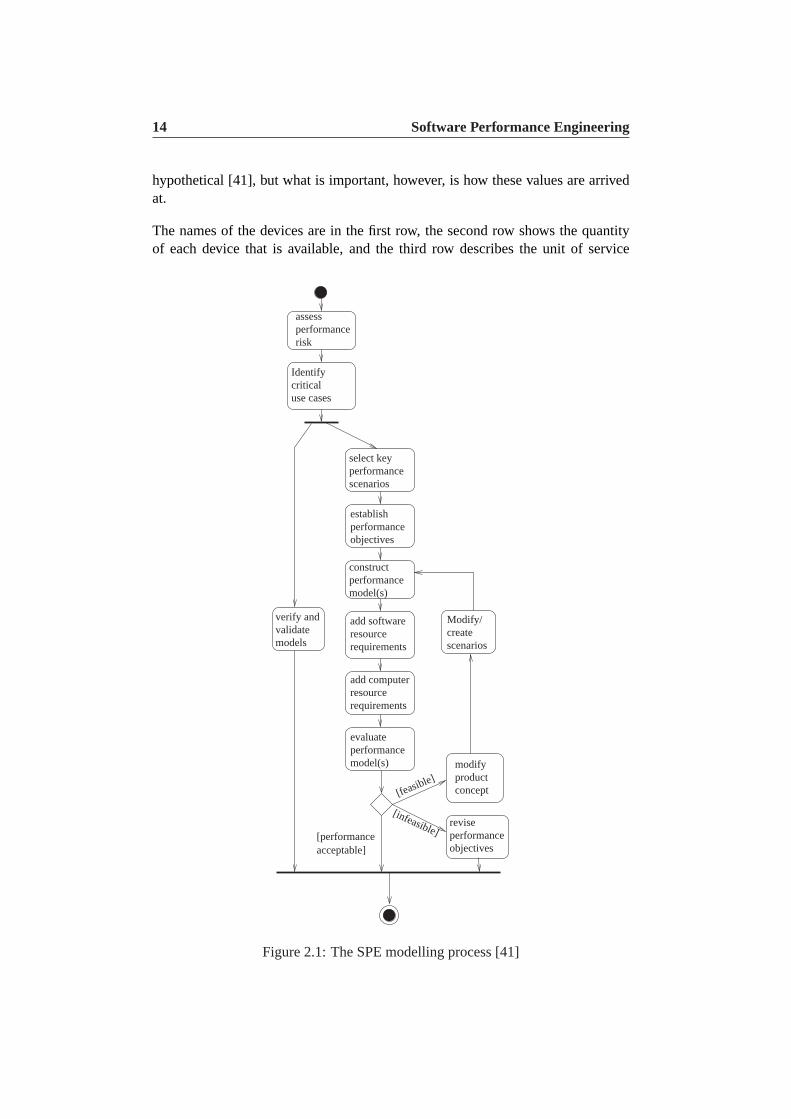
SPE is a systematic approach that proceeds according to a nine step plan describedbelow and illustrated in figure 2.1.
1. Assess performance risk: An assessment of performance risks is done in or-der to determine the amount of SPE effort that is required for a particularproject. Performance risks include familiarity with the type of system thatis to be developed, new technologies, computer and network ressources re-quired, and so forth. A high degree of performance risks implies a greater
12 Software Performance Engineering
deal of effort to be put into SPE activities.
2. Identify critical use cases. The critical use cases are those that are importantto the operation of the system, or that are important to performance as seenby the user, i.e., theresponsivenessof the system. In the UML, use cases arerepresented by use case diagrams
3. Select key performance scenarios. A use case typically consists of severalscenarios. Scenarios are externally visible execution paths which can be ex-pressed in the UML by either sequence-, activity-, or collaboration diagramscapturing the flow of messages being passed between objects. As it is, SPEuses an augmented form of sequence diagrams that includes extensions fordecomposing a scenario into subscenarios, as well as constructs to expresslooping, alternation and optional execution. Typically only a subset of thescenarios constituting a use case will be important from a performance per-spective. The objective is to identify these scenarios. Indications to whichare the key scenarios are those that are executed frequently, or those that arecritical to the perceived performance of the system.
4. Establish performance objectives. Quantitative performance objectives aredefined for each selected scenario in order to evaluate the performance char-acteristics of the system.
The steps 5 through 8 are repeated until there are no outstanding performanceproblems.
5. Construct performance models. SPE uses execution graphs to represent thesoftware processing steps of each the selected performance scenarios. Thesequence diagrams representing these key scenarios are translated to execu-tion graphs.
6. Determine software resource requirements. Software resources are the re-sources affecting the performance of the software. The types of softwareresources to consider depend on the application to be developed and thesoftware that the application interfaces with, so software resources may in-clude CPU, I/O, messages, etc. as well as, say, calls to middleware functionsor functions in different processes. Determining software resource require-ments means establishing the amount of work that is required for each ofthese software resources, for instance how many messages must be sent orhow many CPU instructions are needed to perform a given operation.
7. Add computer resource requirements. The computer resources represent keydevices in the execution environment from which the identified software re-sources require service. Computer resources include CPU time, number ofphysical I/O, size of messages sent and so forth. Information about the exe-cution environment can be obtained from the UML deployment diagram and
13
other documentation. The software resource requirements are mapped ontothe amount of service they require from the computer resources. Computerresource requirements are represented in a so-calledoverhead matrix.
8. Evaluate the models. Solving the execution graph yields the resource re-quirements of the proposed software in isolation, i.e., without consideringexternal factors, such as other programs competing for resources. If the so-lution indicates that there are no performance problems, the next step is tosolve thesystem execution model. The system execution model character-izes the performance of the software in the presence of factors that couldcause contention for resources, such as other programs competing for CPUtime. The system execution model is represented by means of a QueueingNetwork Model (QNM).
9. Verify and validate the models: A continuous verification and validation ofthe constructed models occur in parallel with the actual construction andsubsequent evaluation of the models. Verification and validation answers thefollowing questions: “Are we building the model right” and “are we buildingthe right model”, respectively. Model verification and validation are aimedat determining whether the model predictions provide an accurate reflectionof the software’s performance as well as detect whether there are any modelomissions.
The preceding nine steps describe SPE as it is approached in a single phase of thedevelopment cycle. These steps are applied iteratively for each subsequent phaseof the development process, each cycle resulting in more refined models as thedesign evolves and more information becomes available.
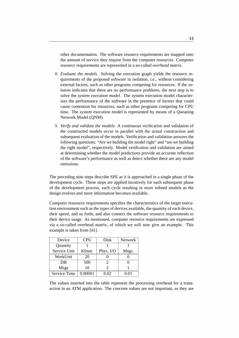
Computer ressource requirements specifies the characteristics of the target execu-tion environment such as the types of devices available, the quantity of each device,their speed, and so forth, and also connect the software resource requirements totheir device usage. As mentioned, computer resource requirements are expressedvia a so-called overhead matrix, of which we will now give an example. Thisexample is taken from [41].
Device CPU Disk NetworkQuantity 1 1 1
Service Unit KInstr. Phys. I/O Msgs.WorkUnit 20 0 0
DB 500 2 0Msgs 10 2 1
Service Time 0.00001 0.02 0.01
The values inserted into the table represent the processing overhead for a trans-action in an ATM application. The concrete values are not important, as they are
14 Software Performance Engineering
hypothetical [41], but what is important, however, is how these values are arrivedat.
The names of the devices are in the first row, the second row shows the quantityof each device that is available, and the third row describes the unit of service
establishperformance objectives
riskperformance assess
Identifycriticaluse cases
modifyproductconcept
performancemodel(s)
evaluate
add softwareresourcerequirements
constructperformancemodel(s)
select keyperformance scenarios
Modify/createscenarios
reviseperformanceobjectives
verify andvalidatemodels
[feasible]
[infeasible][performanceacceptable]
add computer
requirementsresource
Figure 2.1: The SPE modelling process [41]
2.1 Execution Graphs 15
for each of the devices, e.g., a single unit for the CPU corresponds to 1000 CPUinstructions.
The values in the center section of the table defines the mapping between softwareresource requests and device usage. For example, theDB row specifies that eachDB request requires 500K CPU instructions and 2 physical I/Os.Msgs require10K CPU instructions, 2 I/Os, and 1 network message. Finally, eachWorkUnitrequires 20K instructions.
The bottom row specifies the service time for each device.
An overhead matrix is created for each of the key performance scenarios, and thisis used as input when creating the software execution model (Execution Graph)and system execution model (Queueing Network Model). Creating and solvingboth the Execution Graphs and later Queueing Network Models can be performedalgorithmically and commercial tools exist for doing so. However, for the purposeof clarification, we present a brief description of this conversion process.
2.1 Execution Graphs
In order to calculate the accumulated time for a use case, which may consist ofseveral performance scenarios, the sequence diagrams are converted to executiongraphs and the accumulated time is then calculated. In the following we give ahigh-level description of the algorithms that perform this transformation. We startby giving a brief account of an execution graph.
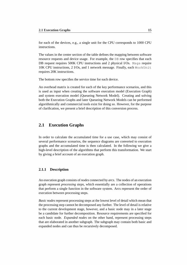
2.1.1 Description
An execution graph consists ofnodesconnected byarcs. The nodes of an executiongraph representprocessing steps, which essentially are a collection of operationsthat perform a single function in the software system. Arcs represent the order ofexecution between processing steps.
Basic nodesrepresent processing steps at the lowest level of detail which mean thatthe processing step cannot be decomposed any further. The level of detail is relativeto the current development stage, however, and a basic node may in a later stagebe a candidate for further decomposition. Resource requirements are specified foreach basic node.Expanded nodeson the other hand, represent processing stepsthat are elaborated in another subgraph. The subgraph may contain both basic andexpanded nodes and can thus be recursively decomposed.
16 Software Performance Engineering
A repetition node, represented by a circle with a diagonal line, denotes a repetitionof one or more nodes.
A case node, represented by a fork-like figure, denotes a conditional execution ofalternate processing steps. It has one or moreattached nodesthat represent thechoices that may be executed. The choices are annotated with their probability ofbeing executed.
Figure 2.2 summarizes the various nodes.
n
Basic node
Extended node
Loop Node
Case Node
Figure 2.2: Basic execution graph nodes
2.1.2 Transforming sequence diagrams to execution graphs
Given that SPE uses an augmented form of sequence diagrams that allow ex-tensions for decomposition, loops and conditional expressions the transformationprocess to execution graphs is straightforward. The most obvious approach to per-forming the transformation is to follow the message arrows through the sequencediagram, and make each action a basic node in the execution graph. However, inmany cases, individual actions may be combined into a single basic node. Alter-natively, an expanded node can be used to summarize a series of actions with thedetails shown in the subgraph.
2.1 Execution Graphs 17
2.1.3 Calculating the time for a use case
Once the performance scenarios constituting a use case have been converted toexecution graphs, the accumulated time of the use case can be calculated. We nowpresent a high-level description of the algorithms that perform this transformation.
The solution algorithms works as follows. The graph is examined and a basicstructure is identified. There are three types of basic structures: sequence struc-tures, denoting sequential execution, loop structures denoting repeated execution,and case structures, denoting conditional execution.
The solution algorithms utilize graph reduction to compute the time: The time forthe structure is computed and replaced by a “computed node” that displays thetime it takes to complete the structure. This process is continued until the graph isreduced to a single computed node, which represent the result of the analysis.
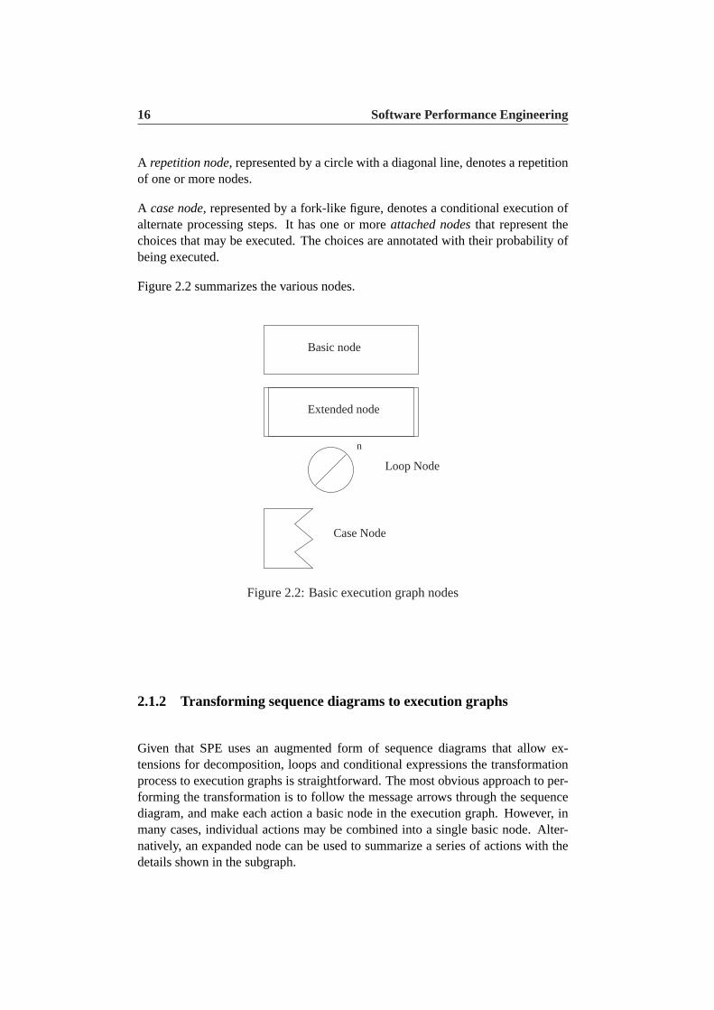
The computed time for a sequence structure is the sum of the times of the nodes inthe sequence. This is illustrated in figure 2.3
t1
t2
tn
t
+ ... ++= t1 t2 t nt
Figure 2.3: Sequence structure
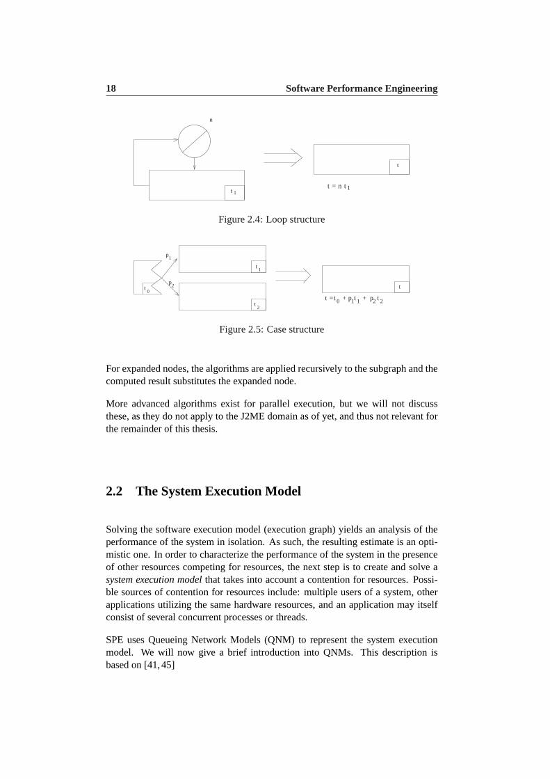
For loop structures, the node time is multiplied by the loop repetition factor. Thisis illustrated in figure 2.4
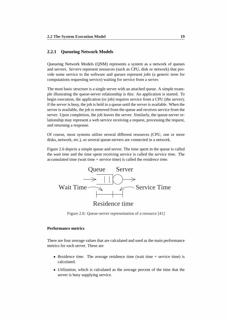
The computation for case nodes is divided into three: shortest path, longest pathand average analysis where the time for shortest path for the case node is the mini-mum of the times for the conditionally executed nodes, while the longest path rep-resent the maximum (or worst case) times. For the average analysis, each node’stime is multiplied with its execution probability. Graph reduction for case nodes isillustrated in figure 2.5
18 Software Performance Engineering
1t
n
t
t n= 1t
Figure 2.4: Loop structure
1
t
t += p1tt 0
t
t2
p
p
t
1
20
1 + p2 2t
Figure 2.5: Case structure
For expanded nodes, the algorithms are applied recursively to the subgraph and thecomputed result substitutes the expanded node.
More advanced algorithms exist for parallel execution, but we will not discussthese, as they do not apply to the J2ME domain as of yet, and thus not relevant forthe remainder of this thesis.
2.2 The System Execution Model
Solving the software execution model (execution graph) yields an analysis of theperformance of the system in isolation. As such, the resulting estimate is an opti-mistic one. In order to characterize the performance of the system in the presenceof other resources competing for resources, the next step is to create and solve asystem execution modelthat takes into account a contention for resources. Possi-ble sources of contention for resources include: multiple users of a system, otherapplications utilizing the same hardware resources, and an application may itselfconsist of several concurrent processes or threads.
SPE uses Queueing Network Models (QNM) to represent the system executionmodel. We will now give a brief introduction into QNMs. This description isbased on [41,45]
2.2 The System Execution Model 19
2.2.1 Queueing Network Models
Queueing Network Models (QNM) represents a system as a network of queuesand servers.Serversrepresent resources (such as CPU, disk or network) that pro-vide some service to the software andqueuesrepresentjobs (a generic term forcomputations requesting service) waiting for service from a server.
The most basic structure is a single server with an attached queue. A simple exam-ple illustrating the queue-server relationship is this: An application is started. Tobegin execution, the application (or job) requires service from a CPU (the server);if the server is busy, the job is held in a queue until the server is available. When theserver is available, the job is removed from the queue and receives service from theserver. Upon completion, the job leaves the server. Similarly, the queue-server re-lationship may represent a web service receiving a request, processing the request,and returning a response.
Of course, most systems utilize several different resources (CPU, one or moredisks, network, etc.), so several queue-servers are connected in a network.
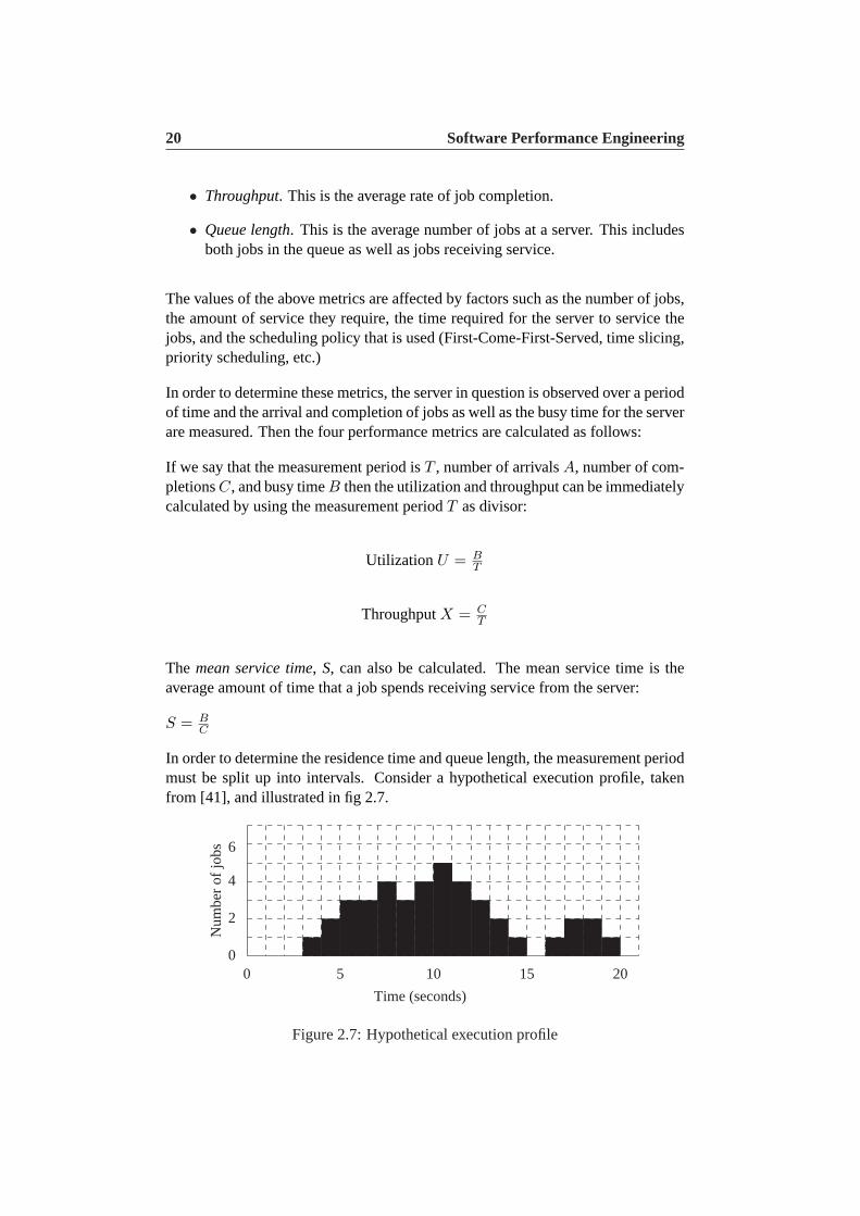
Figure 2.6 depicts a simple queue and server. The time spent in the queue is calledthe wait timeand the time spent receiving service is called theservice time. Theaccumulated time (wait time + service time) is called theresidence time.
Queue Server
Residence time
Service TimeWait Time
Figure 2.6: Queue-server representation of a resource [41]
Performance metrics
There are four average values that are calculated and used as the main performancemetrics for each server. These are
• Residence time. The average residence time (wait time + service time) iscalculated.
• Utilization, which is calculated as the average percent of the time that theserver is busy supplying service.
20 Software Performance Engineering
• Throughput. This is the average rate of job completion.
• Queue length. This is the average number of jobs at a server. This includesboth jobs in the queue as well as jobs receiving service.
The values of the above metrics are affected by factors such as the number of jobs,the amount of service they require, the time required for the server to service thejobs, and the scheduling policy that is used (First-Come-First-Served, time slicing,priority scheduling, etc.)
In order to determine these metrics, the server in question is observed over a periodof time and the arrival and completion of jobs as well as the busy time for the serverare measured. Then the four performance metrics are calculated as follows:
If we say that the measurement period isT , number of arrivalsA, number of com-pletionsC, and busy timeB then the utilization and throughput can be immediatelycalculated by using the measurement periodT as divisor:
Utilization U = BT
ThroughputX = CT
The mean service time, S, can also be calculated. The mean service time is theaverage amount of time that a job spends receiving service from the server:
S = BC
In order to determine the residence time and queue length, the measurement periodmust be split up into intervals. Consider a hypothetical execution profile, takenfrom [41], and illustrated in fig 2.7.
00
6
4
2
5 10 2015
Time (seconds)
Num
ber
of jo
bs
Figure 2.7: Hypothetical execution profile
2.2 The System Execution Model 21
This measurement period last 20 seconds and is divided into one second intervals.Then the number of jobs at the server for each interval,W , is sum up:
W =∑
intervals(#jobs)
In this example, this adds to:
W = 0+0+0+1+2+3+3+4+3+4+5+4+3+2+1+0+1+2+2+1 = 41
The residence time (R) and queue lengthN can now be calculated using W asnumerator:
R = WC
N = WT
As seen, the above calculations of the main performance metrics rely on actualmeasurements. However, the approach of SPE in the early phases of the develop-ment process, is to rely onestimates. The estimates concern the predictedworkloadintensityandservice requirements. Workload is a term denoting the collection ofrequests for service and workload intensity is a measure of the number of requestsmade in a given time interval. Service requirements are the amount of time that theworkload requires from each of the devices.
Types of QNM
There are two types of QNMs: Closed models and open models.
Open models are appropriate for modelling systems where jobs arrive, receivesome service, and then leave the system. An example might be a web service thatreceives a request, processes the request, and then sends a response. For an opensystem theworkload intensityis specified as thearrival rate, that is, the rate atwhich jobs arrive for service. The service requirements are specified as thenumberof visitsfor each device and themean service timeper visit.
In contrast to open models, closed models have no external arrivals or departures.Instead, jobs keep circulating among queues. Closed models are appropriate forinteractive systems where users issue a request, receive a response, and then issueanother request.
22 Software Performance Engineering
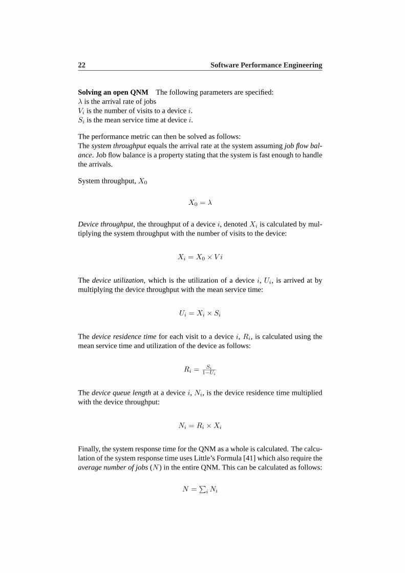
Solving an open QNM The following parameters are specified:λ is the arrival rate of jobsVi is the number of visits to a devicei.Si is the mean service time at devicei.
The performance metric can then be solved as follows:Thesystem throughputequals the arrival rate at the system assumingjob flow bal-ance. Job flow balance is a property stating that the system is fast enough to handlethe arrivals.
System throughput,X0
X0 = λ
Device throughput, the throughput of a devicei, denotedXi is calculated by mul-tiplying the system throughput with the number of visits to the device:
Xi = X0 × V i
The device utilization, which is the utilization of a devicei, Ui, is arrived at bymultiplying the device throughput with the mean service time:
Ui = Xi × Si
The device residence timefor each visit to a devicei, Ri, is calculated using themean service time and utilization of the device as follows:
Ri = Si1−Ui
Thedevice queue lengthat a devicei, Ni, is the device residence time multipliedwith the device throughput:
Ni = Ri ×Xi
Finally, the system response time for the QNM as a whole is calculated. The calcu-lation of the system response time uses Little’s Formula [41] which also require theaverage number of jobs(N ) in the entire QNM. This can be calculated as follows:
N =∑
i Ni
2.3 Other approaches 23
Now the system response time,RT , can be calculated using Little’s Formula asfollows:
RT = NX0
Solving a closed QNM When solving a closed QNM the workload intensity isspecified as thenumber of users(or simultaneous jobs) and thethink time, whichis the average delay between receiving a response and sending the next request.Solving a closed QNM is more complex and the description of this solution isbeyond the scope of this thesis.
Creating and solving the system execution model
We will now give a brief description of the process of creating and solving a systemexecution model.
In order to construct and solve a system execution model, the first step is to addqueue-servers to represent the key computer resources and devices. Then, connec-tions between queues are added. The third step is to decide whether the system ismodeled more appropriate using an open or closed QNM. Fourthly, the workloadintensities for each scenario must be determined. The arrival rate and/or number ofusers is based on an anticipated use of the system and the service times are obtainedfrom the solution to the software execution model. The last step of the process isto specify the service requirements. The device characteristics (processor speed,average time to complete an I/O operation, etc.) come from specifications of theexecution environment while the visits and service times come from the softwareexecution model.
2.3 Other approaches
A number of alternative approaches to early performance evaluation have emergedfrom the SPE foundation. These contributions can be largely divided into twocategories: 1) Those that model performance by alternate means as compared toSPE, and 2) approaches targeted at specific application domains.
24 Software Performance Engineering
2.3.1 Alternate modelling approaches
[24] incorporates activity diagrams into the SPE approach. In addition, theypresent a prototype for a CASE tool that translates model elements from activitydiagrams into a Generalized Stochastic Petri Net (GSPN).
[8] present a methodology that from UML use case diagrams, sequence dia-grams and deployment diagrams produce an Extended Queueing Network Model(EQNM). The methodology includes algorithms for extracting performance as-pects from the UML models and integrating them into the EQNM.
[9] takes a somewhat similar approach in that it relies on information containedin use case diagrams, sequence diagrams and deployment diagrams. The resultingperformance model, however, is a QNM.
[35] propose a graph-grammar based method for transforming performance an-notated UML models into a Layered Queueing Network (LQNM) performancemodel. The transformation takes as input an XML file that describes the UMLmodel according to the XMI (XML Metadata Interchange) [30] interface and out-puts a corresponding LQNM model description file. They rely on a combinationof collaboration diagrams, deployment diagrams, and activity diagrams to expressthe software architecture, the allocation of software components to hardware re-sources, and represent the performance scenarios. They report on problems re-garding the inter-operability with UML tools, since the UML tools do not entirelysupport the UML standard. As a consequence, they had to change the XML filesexported from the UML tools in order to add missing features.
The authors of [35] extend their previous work in this article [14], proposing analternative approach that implements the UML to LQN transformation by usingXSLT (Extensible Stylesheet Language for Transformations) [46]. The input tothe transformation is once again an XML file representation of the UML modeland the output an LQNM description file. They provide a comparison with theirprevious approach concluding that the XSLT transformation approach is faster todevelop. However, their problems with existing UML tools are unresolved.
Lastly, the authors have continued their work from [14,35] in [15]. It directly buildson [14] by using an XML representation of UML models according to the XMIinterface, exported by a UML tool (Rational Rose). The transformation is donevia XSLT, and this time the UML models are transformed into a simulation-basedperformance model (CSIM18 [43]). The work in all three articles is constrained tothe client-server architectural pattern.
2.3 Other approaches 25
2.3.2 Specific application domain approaches
PRIMAmob-UML is an extension of PRIMA-UML [9] specifically targeted at sys-tems that make use of mobile code. To this end PRIMAmob-UML uses an ex-tended UML notation as well as extended EGs and EQNMs to account for mobilecode.
[22] is an example of SPE being applied in the development process of a DigitalSignal Processing a (DSP) application.
[6] applies SPE to web services. The paper has two contributions: 1) it proposesa web services based infrastructure to support Clinical Decision Support Systems(CDSSs) for processing data from multiple medical domains, and 2) it uses SPE toanalyze the performance of the proposed system.
[26] present a methodology for evaluating the performance of the design of client-server systems. They base their methodology on a special software performanceengineering language, developed by one of the authors, calledClisspe (CLIen-t/Server Software Performance Evaluation). A compiler for the Clisspe languagegenerates a performance model (QNM) that can be solved by a model (QNM)solver.
[23] present a trace tool called EXTRA (Executable Trace Files) developed byIBM as part of the Visual Age for C++ product. They show how this tool can beused to generate traces for key performance scenarios of a prototype or a partiallyimplemented systems in order to arrive at estimates which a performance analystcan then map into a Layered Queueing Network Model. These performance scenar-ios are then inserted into another IBM product named the Distributed ApplicationDevelopment Toolkit (DADT) which is used to consider the performance impactof design and configuration changes. These two tools are applied to a case studyof a distributed application system.

3Problemsand proposed
solutions
3.1 Problems with SPE
The greatest problem of adopting SPE as we view it, is the heavy reliance on aperformance specialist being associated to a development project, in order to makeSPE work.
This fact is probably expressed most clearly in step number 7 of the SPE approach:adding computer resource requirements. Adding computer resource requirementsmeans determining the amount of service that is required for various operations.
The overhead matrix representing the computer resource requirements is whatdrives the model solutions, and thus result in the final estimates of the system.
But manually supplying the computer resource requirements constitutes a greatproblem, as we will now illustrate.
In order to determine the approximated time it takes to complete a key task (keyperformance scenario) the amount of CPU instructions must be estimated.
We argue that most system developers/programmers do not have a clear appre-ciation of how many CPU instructions correspond to an operation specified in a
28 Problems and proposed solutions
high-level programming language. For instance, few programmers probably real-ize that a database query may involve several hundred thousands or even millionsof instructions [41]. In order to calculate a correspondence between applicationlines of code and CPU instructions we would need compilable code. Of course,this defers the whole point of estimating performance at an early point. For thesake of argument, let’s assume that we do have compilable code. Even then, differ-ent compilers may generate significantly varying machine code or bytecode, andadvanced compilers may perform optimizations that may be near impossible topredict beforehand.
There is also the problem of information hiding. When using middleware layers,interfaces or externally made components, such as when combining web services,the details of functionality are obscured. This is usually considered good practicefrom a software engineering perspective, but it significantly adds to the complexityof performance analysis.
As a consequence, any estimates which are to be likely predictions of the perfor-mance, requires the presence of a highly competent performance specialist who hasa profound understanding of intricate details of the target environment and relevantsoftware. Maintaining the qualities of such a performance specialist - keeping himup to date with the continuous and rapid emergence of new technologies is a job initself. This also makes the SPE approach inherently people dependent. Maintain-ing this level of performance knowledge in several developers, to account for anypeople departures, is not a feasible option, at least not in smaller organizations.
3.1.1 Reliability of performance predictions
The reliance on a performance specialist also introduces an element of uncertaintyconcerning the reliability of the resulting performance estimates (predictions). Theaccuracy of the resulting performance estimates are a direct function of the levelof expertise of the performance specialist who supplies the input estimates. If theinput estimates supplied by the performance specialist are not reasonably accuratethen nor will the resulting estimates from solving the performance models be. As[40] notes: “Model making requires possibly invalid assumptions”.
3.1.2 SPE and OO
Object-oriented (OO) systems present additional challenges for SPE. Performingan OO function is likely to involve numerous and complex interactions betweenmany different objects making the interactions difficult to trace. This difficulty isfurther compounded by polymorphism [41]. Add to this the advent of exceptions
3.1 Problems with SPE 29
which may cause sudden breaks in the control flow, and the unpredictable perfor-mance spikes incurred by the garbage collector kicking in. These factors contributeto making performance estimations of an OO system extremely difficult.
3.1.3 The cost of SPE
Initially, the input estimates may rely on guesses, and then as the developmentprocess progresses and more information becomes available SPE activities are con-ducted in order to reflect this new knowledge: input estimates are adjusted, perfor-mance models are modified or recreated and the models are verified and validated.
Developing a model manually can be a very labor intensive and error-prone process.Applications may use a host of different hardware and software resources, includ-ing objects, threads, middleware, operating system processes, network, databasesand so forth. Performance modelling needs to consider all these aspects. Further-more, it is a major challenge to ensure that the model remains in sync with anevolving design [23].
This brings up the issue of the cost of implementing SPE. [41] argues that thecost of SPE is minor relative to the overall project cost. According to [41] thecost of SPE at Lucent Technologies range from less than one percent of the totalproject budget for projects with a low performance risk to ten percent of the totalbudget for projects where the performance risk is very high. Arguably, the majorityof companies do not have a project budget that is anywhere near that of LucentTechnologies and the percentage-wise cost for SPE may thus be far greater forsmaller companies.
Moreover, SPE may be a “hard sale”. If an organization is not developing pro-jects/software where performance constitutes a great risk, or has not encounteredperformance problems in previous projects they are probably not prone to makean investment in the adoption of SPE to account for the possible occurrence ofproblems in future projects.
3.1.4 Determining amount of SPE effort
Achieving high quality software is a complex mix of factors that vary betweenprojects. Quality in software encompasses quality attributes such as maintain-ability, flexibility, reusability, efficiency, and determining which ones should beemphasized in a particular project depend on the application to be built and thecustomer who requested it [36]. High performance may not be the most importantcriteria for success, so including SPE activities into every project may not be rel-evant. [41] notes that the amount of SPE effort must be evaluated beforehand and
30 Problems and proposed solutions
if the performance risk is low, the SPE effort should reflect this. However, deter-mining the correct amount of SPE effort requires experience and a knowledge ofissues that may prove problematic from a performance perspective.
3.1.5 The need for quantitative requirements
According to the SPE approach, quantitative requirements should be establishedfor all key performance scenarios. This information should be supplied by a sys-tem architect in collaboration with a performance engineer as well as a marketingrepresentative and/or a user representative.
As we see it, the demand for establishing quantifiable requirements present a prob-lem as well. The customer (represented be a user representative) may very well bea non-technical person who does not have an appreciation of the amount of workbehind each processing step, and will maybe accept no less than the ideal. The cus-tomer may not have a clear appreciation of how long say, 2 seconds waiting timeis. This may sound acceptable to the customer (representant), but may prove asan unacceptable waiting time to actual end users. Moreover, if we take the perfor-mance engineer out of the equation for one minute, “ordinary” system developersmay not have a clear understanding at this point either of the amount of work (interms of exact, or even approximate, time measures) that is required for variousparts of the system. Thus, they may inadvertently commit to response times, thatmay later prove impossible to obtain.
This situation clearly illustrates the necessity of a performance engineer beingpresent who hopefully have enough experience to provide reasonably realistic es-timates, and who is able to convey the arguments of why various parts take as longtime as they do, in order to convince the customer.
If it turns out that the specified objectives can not be met, SPE states that an alterna-tive may be to renegotiate the objectives with the customer. However, we find thatsuch a tactic may damage customer relations, particularly if this situation occursrepeatedly throughout the development process. Even if the customer complies tothe new objectives, we feel such a tactic may leave an impression of unprofessionalconduct.
Lets say that the system to be built should start by collecting data from a server.This may be an action that should be performed once a day, say at the start of thework day. It may be the case that this fetching time really isn’t that important, if theend user can use the waiting time to get or cup of coffee or something. In such acase, committing to a fetch time of say 10 seconds may be overly constrained, whenin fact the user could easily tolerate, say, one minute, where the user is occupieddoing other things. The process of trying to achieve these 10 seconds may prove
3.1 Problems with SPE 31
impossible, necessitating a renegotiation, when in fact this could be avoided bylistening to what is the typical workday scenario of the end user is.
3.1.6 Software Engineering and SPE
SPE has not yet been incorporated into the practices of Software Engineering (SE)[27]. The author of [27] point to a lack of scientific principles and models in SE,a lack of education in performance, and an IT workforce employing many peoplewith less than a bachelors degree and no formal training as possible causes asto why performance is not considered at the design time in software engineeringprojects.
[21] has conducted a survey of undergraduate computer science courses at highlyranked computer science schools in the United States (the top 24 research and doc-torate schools according to data from Computer Research Association’s TaulbeeSurvey [21]) in order to find out what kind of education undergraduates are re-ceiving with respect to designing, building, and maintaining software that exhibitsgood performance. The survey was aimed at the undergraduate level, since theyrepresent the majority of the workforce - only about 20 percent of the computerscientist students receive a graduate degree.
The survey indicated a number of shortcomings, including:
• Performance was rarely discussed (64.87% of the software engineering coursesspend little or no time discussing performance-related subjects)
• In the cases where performancewasdiscussed, the subject was either inade-quately or not defined (84.84% of the courses had an inadequate or missingperformance definition)
• Performance was regarded as a late life cycle activity (72% of the coursesadvocated a reactive strategy to performance).
• In most cases performance was viewed as a low-level system or algorithmicproblem (74.07% of the courses regarded low-level system components oralgorithmic efficiency as having the greatest impact on application perfor-mance.)
• Not a single course discussed how to measure resource utilization (no tech-niques for measuring throughput and utilization of resources)
• Only few of the courses (27.02%) discussed performance modelling. Ofthese courses, half used models for performance validation before imple-mentation while the other half used models to diagnose problems in an im-plemented system.
32 Problems and proposed solutions
• SPE was only mentioned in two courses, and one of these incorrectly impliedthat SPE was a specialized discipline for database-centered and real-timeapplications.
Since performance issues have traditionally been considered a late life cycle ac-tivity, SPE is not reflected in the mainstream process models [38]. [38] point to anumber of problems in the mainstream process models that adversely effects theintegration of SPE into SE and propose an extension that explicitly takes SPE ac-tivities into account.
However, integrating SPE into SE is contingent on the appropriate amount of per-formance knowledge being available, which the survey [21] shows may far fromalways be the case.
As a result, achieving widespread use of SPE would entail a reorganization of thecomputer science courses being taught at the majority of universities, as well as anew or extended process model that explicitly takes SPE into account.
We do not regard these two conditions to be realistically met in the near future andas a consequence early performance considerations must rather be be adapted intothe existing SE paradigm instead of vice versa.
3.2 Proposed solutions
We propose an alternative to the SPE way of estimating performance. Motivated bythe problems with SPE, described in the previous section, we propose an approach,that is easily integrated into the software engineering domain.
This approach is realized by making a test application that captures performancecharacteristics of the execution environment. The user (developer) uses the testapplication to obtain performance measurements of a series of relevant operationsexecuted on the target device. The results from these tests are then used as inputto a performance annotated UML activity diagram. In order to remain compli-ant with the recent advances in UML performance annotations, we rely on theUMLTM Profile for Schedulability, Performance, and Time Specification (UML-SPT) for annotating the activity diagrams. The annotated diagrams can be exportedinto XML, and the XML representation of the model can then be used as input to aperformance analysis tools which generates and solves an appropriate performancemodel and reports the result back into the appropriate UML tool.
Our objective is to make performance evaluation of systems in the design phase:
3.2 Proposed solutions 33
Usable in that developers do not require extensive knowledge of the multitudeof different devices that applications can be developed to, nor knowledgeof the amount of processing that various high-level operations incur on theunderlying architecture.
Transparent by hiding details of performance model construction and solutionfrom the developer.
Reliable by removing the issue of whether the input estimates supplied by theperformance specialist can be trusted. By using a test application instead weshould be able to obtain consistently reliable estimates.
Cost-efficient as costs associated with manually constructing, solving and laterupdating or recreating performance models, as well as costs associated withspecialized performance staff, are saved.
Collectively, these advantages clearly make early performance validation signifi-cantly more amenable to incorporation into the mainstream practices of softwareengineering.
Regarding the issue of establishing quantitative requirements for all key perfor-mance scenarios that SPE advocates, we advice against it. Performance has tradi-tionally been treated as a non-functional requirement [27, 36, 44], meaning that itis not directly concerned with the specific functions delivered by the system (i.e.,not expressed as an explicit requirement). Rather, non-functional requirements re-late to the system as a whole and are implicitly assumed to be satisfactory (e.g.,showing satisfactory performance). By making performance a functional require-ment we further rely on a skillful performance specialist (to establish reasonablerequirements) which is the situation we are trying to avoid.

4UMLTM Profile forSchedulability,
Performanceand Time
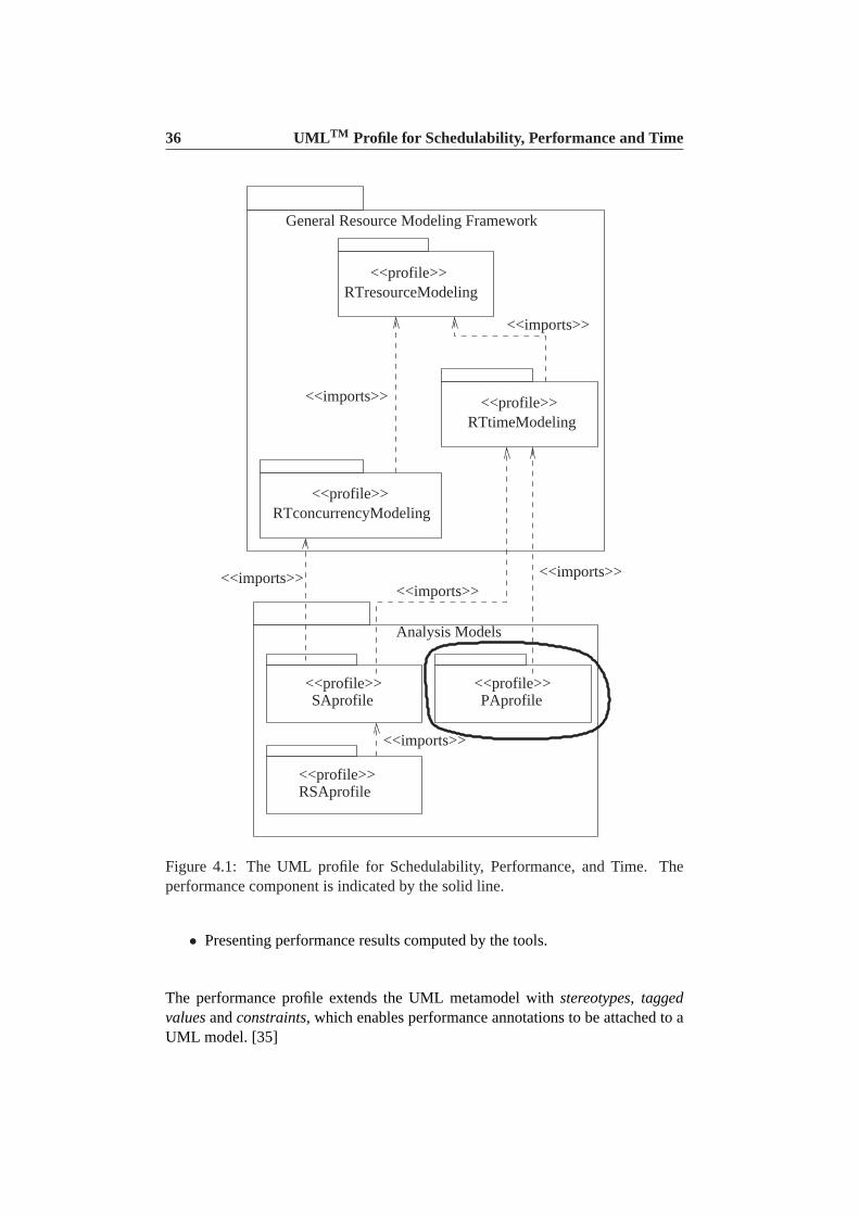
The UMLTM profile for Schedulability, Performance, and Time [13] (UML-SPT) isa UML profile that extends the standard UML with notions for modelling schedu-lability, performance, and time. The point of interest for this thesis is the perfor-mance component of the profile which is used for general performance analysisof UML models. Figure 4.1 illustrates the entire profile graphically, and the areaenclosed by a solid line indicates the place of the performance component in theUML-SPT profile. The main source of information on the performance componentis derived from [13].
The performance component of the profile provides facilities for:
• Capturing quantitative performancerequirements.
• Associating performance-relatedQuality of Service(QoS) characteristicswithselected elements of an UML model.
• Execution parametersto allow modelling tools to compute predicted perfor-mance characteristics.
36 UMLTM Profile for Schedulability, Performance and Time
RTresourceModeling<<profile>>
<<profile>>RTtimeModeling
<<imports>>
<<profile>>RTconcurrencyModeling
Analysis Models
<<profile>>RSAprofile
<<imports>>
<<profile>>SAprofile
<<profile>>PAprofile
<<imports>><<imports>>
General Resource Modeling Framework
<<imports>>
<<imports>>
Figure 4.1: The UML profile for Schedulability, Performance, and Time. Theperformance component is indicated by the solid line.
• Presenting performance results computed by the tools.
The performance profile extends the UML metamodel withstereotypes, taggedvaluesandconstraints, which enables performance annotations to be attached to aUML model. [35]
4.1 Performance analysis of a UML model 37
A Stereotypeis a construct that allows the creation of new model elements thatare specific to a particular domain, such as performance. A stereotype isrepresented as a string enclosed in guillemets («»). An example might bea stereotype «processor »that indicates that this model element represents aprocessor.
A tagged valueconsists of a tag and value, that allows the specification of addi-tional properties for a model element. The tag is the name of the property andthe value field is the value for that property. The UML-SPT profile definesa formal language, called Tagged Value Language (TVL), for specifying thevalue. TVL is based on a very limited subset of the Perl programming lan-guage and the syntax should be familiar to most programmers (we refer toAppendix A of [13] for a description of TVL). A tagged value is enclosed bybraces and appears as follows: {<tag-name> = <TVL-expression>} . An ex-ample might be a tagged value {processorSpeed = 1800Mhz} that is attachedto a model element stereotyped by the aforementioned «processor »stereo-type, indicating that the processor has a processor speed of 1800 Mhz.
A constraint is a restriction or condition which may be placed on an individualmodel element or a collection of elements. The constraint is enclosed bybraces ({}) and interpreted according to a language which may be: the UMLObject Constraint Language; a programming language (e.g., C++ or Java); aformal notation; or a natural language [41]. An example of a constraint maybe this: {responseTime < 200}.
In the performance domain, stereotypes and tagged values can be used to cap-ture information about the execution environment (e.g., processor speed, networkspeed, etc) while constraints can be used to specify performance requirements.
4.1 Performance analysis of a UML model
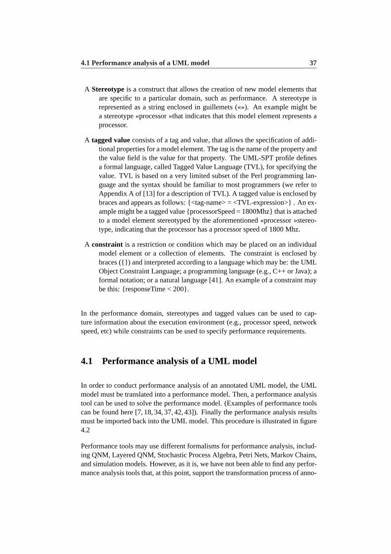
In order to conduct performance analysis of an annotated UML model, the UMLmodel must be translated into a performance model. Then, a performance analysistool can be used to solve the performance model. (Examples of performance toolscan be found here [7, 18, 34, 37, 42, 43]). Finally the performance analysis resultsmust be imported back into the UML model. This procedure is illustrated in figure4.2
Performance tools may use different formalisms for performance analysis, includ-ing QNM, Layered QNM, Stochastic Process Algebra, Petri Nets, Markov Chains,and simulation models. However, as it is, we have not been able to find any perfor-mance analysis tools that, at this point, support the transformation process of anno-
38 UMLTM Profile for Schedulability, Performance and Time
Figure 4.2: Abstract view of the model processing process [13]
tated UML models into input to the performance analysis tools. Rather, the toolswe have cited above rely on a user supplying input manually. Granted, attemptshave been made to try and automate, at least the first step, of the transformationprocess [8,14,15,24,35,49] but the work has not resulted in tools for general use.The backward process (supplying the results of performance solutions back intothe UML model) appear to be uninvestigated [35] at this point, meaning that theperformance modelling of UML diagrams still require knowledge of creating andsolving the appropriate performance models.
4.2 Concepts and techniques
The concepts and techniques of performance analysis in the UML-SPT realm re-semble those which we have already introduced in Chapter 2. Ascenariodefinesan execution path which has a response time and throughput. Each scenario is ex-ecuted by aworkload(collection of requests) with an appliedworkload intensity.An openworkload has a stream of requests (or jobs) that arrive in a predefined pat-tern in which case the workload intensity denotes the arrival rate of the requests,whereas aclosedworkload has a fixed number of jobs that cycle between executingthe scenario and spending an external delay period (think time) between receivinga response and issuing the next request. In this case the workload intensity is thenumber of users/simultaneous jobs and thethink time.
A scenario consists of a number ofscenario stepsthat are joined in a sequence witha predecessor-successor relationship. Steps may be connected via forks, joins andloops and a step may thus have multiple predecessors and successors. A step maybe an elementary operation that cannot be decomposed any further or may be anoperation that is defined by a sub-scenario.
To each step is assigned a mean execution count which is a measure of the averageamount of times the step is repeated when it is executed. A step also has ahostexecution demandwhich is the execution time of the step on its host device in a
4.2 Concepts and techniques 39
given deployment.
The resource demandsby a step include its host execution demand as well as thedemands of all its sub-steps.
Resourcesare modelled asservers. Resource-operationsof a resource are the steps,or sequence of steps which use the resource, consisting of the stages of acquiring,utilizing and releasing the resource. Resource-operations are thus similar to thequeue-serverrelationship introduced earlier.
Theservice timeof a resource is defined as thehost execution demandof the stepshosted by the resource.
Performance measuresfor a system include resource utilizations, waiting times,execution demands (what SPE calls service requirements, e.g., CPU cycles), andthe response times to execute a scenario or scenario step. Each measure may bedefined in different versions:
Required value : A performance objective established for a scenario of scenariostep. This value may originate directly from system requirements or from aperformance estimate based on the requirements.
Assumed value : This value is supplied based on experience.
Estimated value : This value is calculated by a performance tool and reportedback into the model.
Measured value : This value is obtained by conducting actual measurements.
The value of any of the above versions may be stated as one of several statisticalproperties, for instance, the mean or maximum value.
4.2.1 Domain model
Figure 4.3 shows the general performance model that identifies the basic abstrac-tions and relationships used in performance analysis in the UML realm.
Performance context
A common usage of performance analysis tools is to analyze the system undervarying conditions with different parameters while maintaining the same systemstructure. This way, the performance of the system can be estimated, accounting
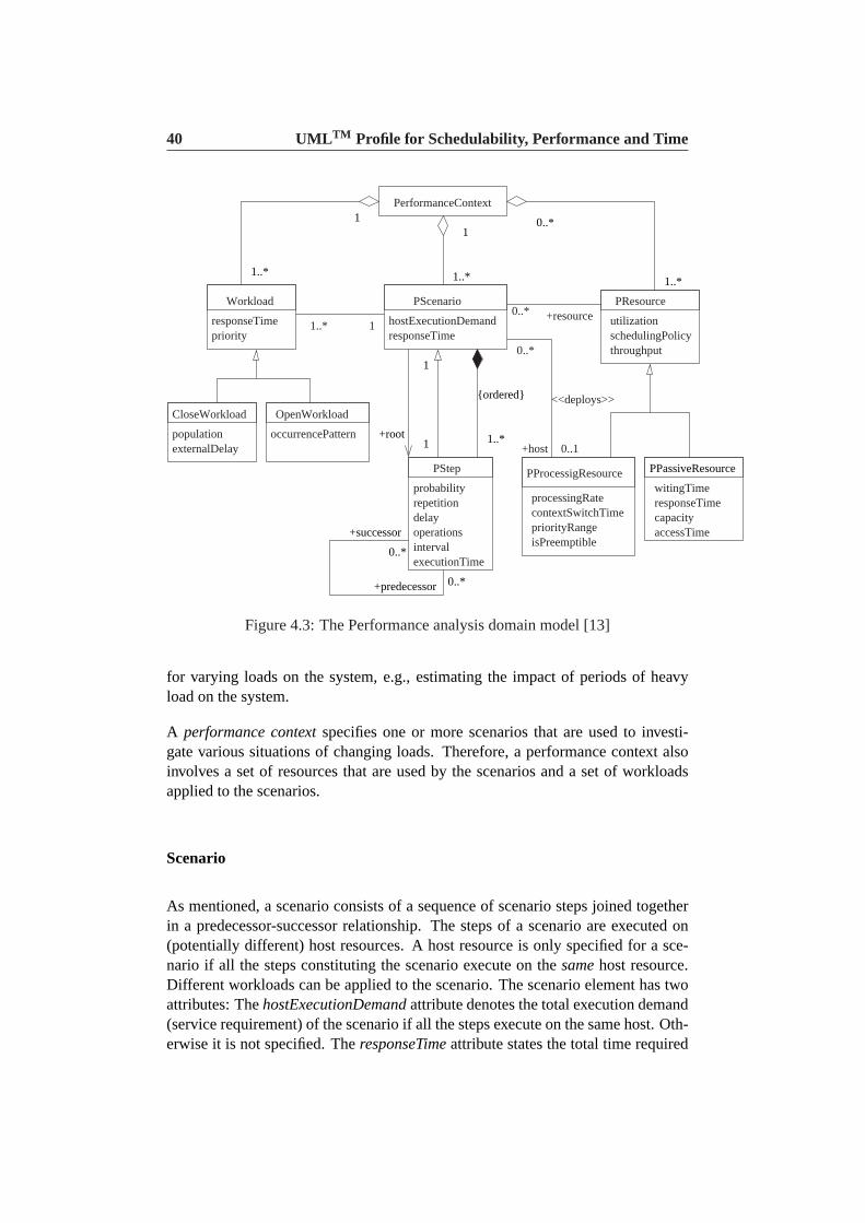
40 UMLTM Profile for Schedulability, Performance and Time
probabilityrepetitiondelayoperationsintervalexecutionTime
PStep
hostExecutionDemandresponseTime
PScenario
1..* 10..* +resource
0..1
<<deploys>>
+host
0..*
processingRatecontextSwitchTimepriorityRangeisPreemptible
PProcessigResource
responseTimecapacityaccessTime
witingTime
occurrencePattern
OpenWorkloadCloseWorkload
populationexternalDelay
utilizationschedulingPolicythroughput
PResource
priorityresponseTime
Workload
PerformanceContext1
1
1..*
1
1
{ordered}
1..*
PPassiveResource
+root
0..*
1..*1..*
0..*
0..*
+predecessor
+successor
Figure 4.3: The Performance analysis domain model [13]
for varying loads on the system, e.g., estimating the impact of periods of heavyload on the system.
A performance contextspecifies one or more scenarios that are used to investi-gate various situations of changing loads. Therefore, a performance context alsoinvolves a set of resources that are used by the scenarios and a set of workloadsapplied to the scenarios.
Scenario
As mentioned, a scenario consists of a sequence of scenario steps joined togetherin a predecessor-successor relationship. The steps of a scenario are executed on(potentially different) host resources. A host resource is only specified for a sce-nario if all the steps constituting the scenario execute on thesamehost resource.Different workloads can be applied to the scenario. The scenario element has twoattributes: ThehostExecutionDemandattribute denotes the total execution demand(service requirement) of the scenario if all the steps execute on the same host. Oth-erwise it is not specified. TheresponseTimeattribute states the total time required
4.2 Concepts and techniques 41
to execute the scenario.
Step
A step indicates an increment in the execution of a scenario and a step is relatedto other steps in the aforementioned predecessor-successor relationship. A stepis specific to a certain scenario and in general a step takes finite time to execute.A step may describe an operation of any level of granularity appropriate for thecurrent modelling effort. Later, the step may be decomposed into finer-grainedsteps. Consequently, scenario steps are modelled as a sub-type of scenarios whichallows for a hierarchical decomposition of scenarios. A step has the followingattributes:
• hostExecutionDemand(inherited from Scenario). If a step is defined at thefinest granularity it executes on a unique host resource and this is the totalexecution demand of the step on the resource. Otherwise, if the step hasa decomposition into a sub-scenario, this is the total demand of the sub-scenario, assuming that all the steps constituting the sub-scenario execute onthe same host.
• delay. This is an inserted delay (e.g., think time) within the step.
• probability. In cases where the predecessor of a step has multiple successors,this is the probability of this step being executed.
• interval. If a step is repeated within a scenario, this is the interval betweenrepetitions of the step.
• repetition. If a step is repeated within a scenario, this is the number of timesthe step is repeated.
• operations. This specifies operation on resources that are not explicitly rep-resented in the model. Instead, these resources are resolved by the appropri-ate performance analysis modelling tool.
Resource
This is an abstract view of a resource which may be eitherpassiveor active. Wewill discuss active and passive resources in the following. A resource may partic-ipate (be utilized) in one or more scenarios of a performance context. A resourcehas the following attributes:
42 UMLTM Profile for Schedulability, Performance and Time
• utilization. The value of this attribute is often supplied as the result of modelanalysis (e.g., solving a QNM) and indicates the average percent of the timethat the resource is being utilized.
• throughput. This is the average rate at which the resource perform its func-tion.
• schedulingPolicy. This is the scheduling policy in effect for accessing theresource.
ProcessingResource
A processing resource is a device such as a processor, interface device or storagedevice. A processingResource has the following attributes:
• processingRate, which is the relative speed factor for the processor.
• contextSwithTime. This is the amount of time it takes for the processingresouce to switch from the execution of one scenario to a different one.
• priorityRange. This is the permissible range of priorities with which re-source actions can be executed.
• isPreemptible. This is a boolean value that indicates if the processor is pre-emptible once it begins execution of an action.
Passive Resouce
A passive resource is a resource that is protected by an access mechanism. Con-current access to the resource is restricted according to some access control policy.The following attributes characterizes a passive resource:
• capacity. This is a measure of the maximum amount of concurrent users ofthe resource.
• accessTime. This is the delay period a scenario incurs when acquiring andreleasing the resource.
• utilization. Utilization for a passive resource is expressed as the averagenumber of concurrent users of the resource.
• responseTime. This is the total amount of time elapsed from the point ofacquiring the resource until the point of releasing the resource.
4.2 Concepts and techniques 43
• waitingTime. This is the elapsed time from a resource request until the re-quest is granted.
Workload
Workload is an abstraction that specifies the execution demand for a a given sce-nario. In addition, required or estimated response time for the scenario pertainingto this workload is given. A workload can be either open or closed. The attributesof a workload are:
• responseTime. The total amount of time from the corresponding scenario isstarted until it is completed.
• priority. This is the priority of the workload.
OpenWorkload
As mentioned, an open workload is characterized by requests arriving continuouslyinto the system at a fixed rate. An openWorkload has a single attribute:
• occurencePattern. This denotes the interval between arriving requests.
ClosedWorkload
In a closed workload, a fixed number of jobs (or users) cycle between executingthe scenario and spending an external think time delay. The attributes are:
• population. This is the size of the workload (number of users/jobs)
• externalDelay. This is the think time delay, i.e., the delay between the endof one response and the start of the next.
The next section describes how the concepts of the performance domain model aremapped to extensions to the UML metamodel.
4.2.2 Mapping the domain model
Scenarios can be modelled as either activity- or collaboration diagrams. In our ap-proach, we will be using activity diagrams to model scenarios, so we will concen-
44 UMLTM Profile for Schedulability, Performance and Time
trate the discussion on mapping the performance concepts onto UML extensionsto an activity diagram. As mentioned, the extensions to the UML metamodel isexpressed via stereotypes, tagged value and constraints.
Using activity graphs, as opposed to using collaboration diagrams, gives the ad-vantage that a scenario can be decomposed into a hierarchical structure, that is, anactivity graph may consist of several lower-level activity graphs.
PerformanceContext
A performance context can be modelled by an activity diagram stereotyped by the«PAcontext»stereotype. (All extension element names of the performance portionof the UML-SPT profile are prefixed with “PA”.) We will defer a discussion of thedetails of the extension elements, but instead refer to [13] for further details. In caseof a scenario containing lower-level activity graphs, only the performance contextof the topmost level can have a workload defined. A requirement concerning theactivity diagram is that the swimlanes can only be used to represent the resourcesused or the object instances participating in the activity.
Scenario
Scenarios are modelled by the activities (also called states or actions) and transitionbetween activities of the activity graph. The UML-SPT profile does not define anexplicit scenario stereotype, but instead identifies the scenario by the first step (rootstep) of the scenario. Also, workload information is attached to the root step.
Step
Each activity or sub-activity of the activity graph is stereotyped as a «PAstep».Workload information can be attached to a step if it is the root step of the top-most performance context. This workload is then imposed on steps of lower-levelperformance contexts.
Workload
The workload for a scenario is modelled by a tagged value associated with theroot step of the topmost performance context. Optionally, the root step can bestereotyped as a «PAOpenLoad»or «PAClosedLoad».
4.2 Concepts and techniques 45
ProcessingResouce
A processing resource can be modelled in two ways. Either by associating theappropriate stereotype «PAhost»with a partition (swimlane). This approach, how-ever, is only appropriate in situations where where each instance is executing on itsown host. Alternatively, in cases where swimlanes represent instances executingon different hosts, and some instances may share hosts the activity diagram can becoupled with a deployment diagram. This is the most common situation.
PassiveResource
Passive resources are represented by swimlanes stereotyped with the «PAresource»stereotype.


Part II
Our Approach

5Describingour approach
Our approach, in this thesis, is targeted at performance on the J2ME platform. Themotivation for choosing the J2ME platform is that device characteristics are verylimited and applications are thus particularly susceptible to performance degrada-tions. Two areas in particular present a challenge on the J2ME platform: networkusage and persistence. There are widely differing performance characteristics be-tween local and remote operations and similarly between operations using persis-tence and operations that do not. These effects are further compounded on theJ2ME platform. Therefore, these two areas are the focus in this thesis.
5.1 The Record Management System
Persistence in J2ME is implemented via the Record Management System (RMS),an API that provides applications with local, on-device persistence. As the nameimplies, data are saved into records, which can be a somewhat misleading termsince records does not contain any fields. Rather, data are saved into a record asan array of bytes. It is not possible to change selected parts of a record - insteadan entire record must be read, changes to the data must be made in memory, andfinally the entire record must be written back [12].
A record can be used to store the state of a class (i.e., the value of its fields) persis-tently by converting the fields of the class into a byte array which is inserted into arecord.
50 Describing our approach
Records are logically collected in to record stores. In order to work on a recordstore it must be first be opened. Correspondingly, an open record store must atsome point be closed.
5.2 Networking
Use of networking on a mobile device can prove problematic due to the limitednetwork bandwidth. There are a few different way a mobile device can access theinternet. The most common ways is through either GSM-CSD, which operates at9,6 kbps or GSM-GPRS which has a theoretical maximum of 172 kbps. Further-more standards like EDGE which operates at speed upto 55 kbps and HSCSD at28.8 kbps also exist. The new 3G standard which is becoming increasingly morewidespread operates at speeds upto 384 kbps depending on how you are positionedin relation to the antenna. These speeds does however not match the speed of wirednetworks which operates at speeds between 512 kbps and several mbps for the typ-ical ADSL connection and between 10 mbps and 1gbps for local area networks.
In this installment we are using web services. Web services are supported by theJSR-172 API in J2ME. However at the present time the JSR-172 API has onlybeen adopted by very few devices - as an example Nokia only has developed threephones so far supporting the JSR-172 API, the N70, N90, and N91 [1–3] and theseare still rather expensive. As a consequence, in order to communicate with webservices on mobile devices third party libraries must be used. In this thesis wehave focused on the use of kSOAP 1.2 [16, 17] as the web service library used tocommunicate with web services.
5.3 Obtaining input estimates
We have created a test application which tests the performance characteristics ofthe RMS and networking.The test application can be used by a developer to obtain input estimates which areused to annotate the activity diagrams.
5.3.1 Testing the RMS
The RMS part of the test application allows the developer to specify the numberof record stores, the number of records in each record store and the size of eachrecord.
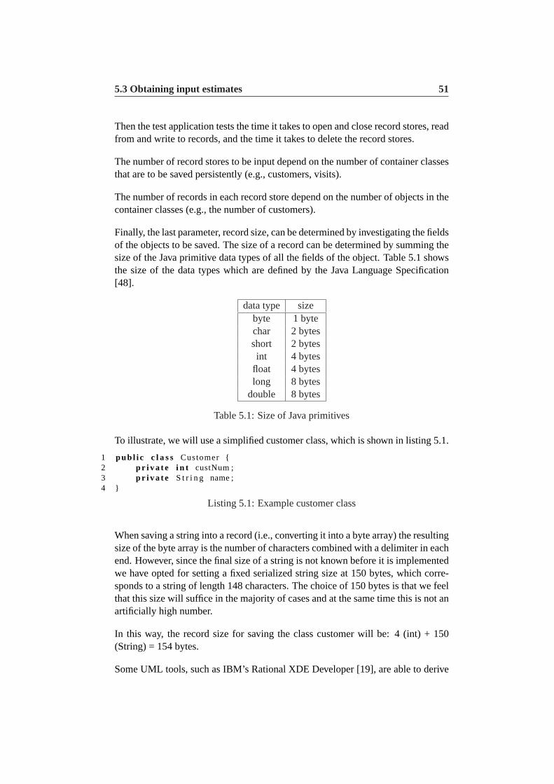
5.3 Obtaining input estimates 51
Then the test application tests the time it takes to open and close record stores, readfrom and write to records, and the time it takes to delete the record stores.
The number of record stores to be input depend on the number of container classesthat are to be saved persistently (e.g., customers, visits).
The number of records in each record store depend on the number of objects in thecontainer classes (e.g., the number of customers).
Finally, the last parameter, record size, can be determined by investigating the fieldsof the objects to be saved. The size of a record can be determined by summing thesize of the Java primitive data types of all the fields of the object. Table 5.1 showsthe size of the data types which are defined by the Java Language Specification[48].
data type sizebyte 1 bytechar 2 bytesshort 2 bytesint 4 bytes
float 4 byteslong 8 bytes
double 8 bytes
Table 5.1: Size of Java primitives
To illustrate, we will use a simplified customer class, which is shown in listing 5.1.
1 pub l i c c l a s s Customer {2 p r i v a t e i n t custNum ;3 p r i v a t e S t r i n g name ;4 }
Listing 5.1: Example customer class
When saving a string into a record (i.e., converting it into a byte array) the resultingsize of the byte array is the number of characters combined with a delimiter in eachend. However, since the final size of a string is not known before it is implementedwe have opted for setting a fixed serialized string size at 150 bytes, which corre-sponds to a string of length 148 characters. The choice of 150 bytes is that we feelthat this size will suffice in the majority of cases and at the same time this is not anartificially high number.
In this way, the record size for saving the class customer will be: 4 (int) + 150(String) = 154 bytes.
Some UML tools, such as IBM’s Rational XDE Developer [19], are able to derive
52 Describing our approach
and present the size of classes based on a class diagram.
5.3.2 Testing the network
On a wireless device the process of requesting data from a web service usingkSOAP consists of these four parts:
1. Creating a SOAP message to send to the web service.
2. Calling the webservice with the SOAP message just created.
3. Getting the result from the webservice.
4. Converting the received SOAP message into an appropriate data structure tobe used in the application.
The test application measures the total amount of time it takes from the point ofcreating the SOAP message until the received SOAP message is converted intoan appropriate data structure. The reason for this approach is that it allows thedeveloper to performance model the application without any knowledge about howthe SOAP message is generated, sent, parsed, and converted into a data structures.
As the overall load of the network, both data and speak, has an effect on the band-width available at any given time, it is imperative that the network test be conductedat a time of the day that is representative of the users “usage pattern”. Obviously,conducting tests at a time that does not correlate to the actual use of end usersproduces results that may give a false indication as to the performance of networkoperation times. For instance, the load between 8 a.m. and 9 a.m., when a lot ofpeople are just starting their workday, can be expected to be greater than the loadbetween 2 a.m. and 3 a.m.
5.4 Using the results
The results obtained from running the test application are used to annotate theactivity diagrams describing the scenarios of a system with respect to operationson the RMS and network. Then the performance annotated diagrams are used toderive performance estimates of the system based on the algorithm for computingExecution Graphs(EG). EGs will suffice since their is no contention for resourceson a J2ME device, and the web service that is contacted is treated as a black-box.
We deliver the results of the tests as three statistical properties: The average, max-imum and 95th percentile [47] response times. The reason for including the 95th

5.4 Using the results 53
percentile is that it is generally less sensitive to odd spikes in the response time thanthe average value can be. This is however only true if the data set is sufficientlylarge.

6Applying ourapproach
In this chapter we will give an example of how the input estimates from the testapplication are used to annotate the activity diagrams describing the scenarios ofthe system. We will also illustrate how the input estimates are used as a basis forcomputing the performance predictions. As a test case we will be using a systemthat we developed as part of a previous project in the fall of 2004 [28].
6.1 A description of the test case
The test case is an end-to-end system consisting of a J2ME application communi-cating with a web service. It is a package registration system developed to aid alogistics company in keeping track of their package elements. The logistics com-pany functions as a central storage for a number of wholesale dealers (customers)and the aim of the system is to help optimize the process of registering packageelements that are used to transport goods as they move from the logistics companyto the wholesale dealers and back again.
The scenario is this:At the warehouse of the logistics company products that are to be shipped out, arepackaged and loaded onto a truck. The truck driver receives a route of where theproducts are to be delivered. At each customer along the route the truck driverdelivers the products (and the package elements used to carry the products) and inreturn he loads onto the truck empty package elements from the customer which he
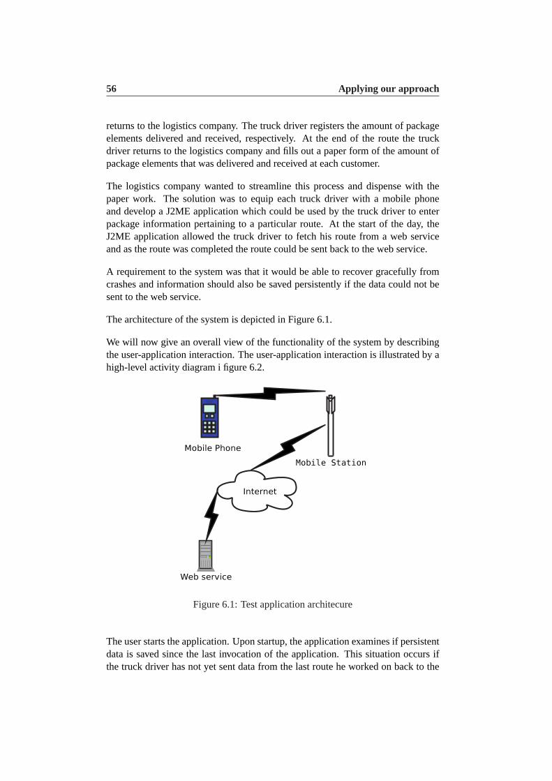
56 Applying our approach
returns to the logistics company. The truck driver registers the amount of packageelements delivered and received, respectively. At the end of the route the truckdriver returns to the logistics company and fills out a paper form of the amount ofpackage elements that was delivered and received at each customer.
The logistics company wanted to streamline this process and dispense with thepaper work. The solution was to equip each truck driver with a mobile phoneand develop a J2ME application which could be used by the truck driver to enterpackage information pertaining to a particular route. At the start of the day, theJ2ME application allowed the truck driver to fetch his route from a web serviceand as the route was completed the route could be sent back to the web service.
A requirement to the system was that it would be able to recover gracefully fromcrashes and information should also be saved persistently if the data could not besent to the web service.
The architecture of the system is depicted in Figure 6.1.
We will now give an overall view of the functionality of the system by describingthe user-application interaction. The user-application interaction is illustrated by ahigh-level activity diagram i figure 6.2.
Figure 6.1: Test application architecure
The user starts the application. Upon startup, the application examines if persistentdata is saved since the last invocation of the application. This situation occurs ifthe truck driver has not yet sent data from the last route he worked on back to the
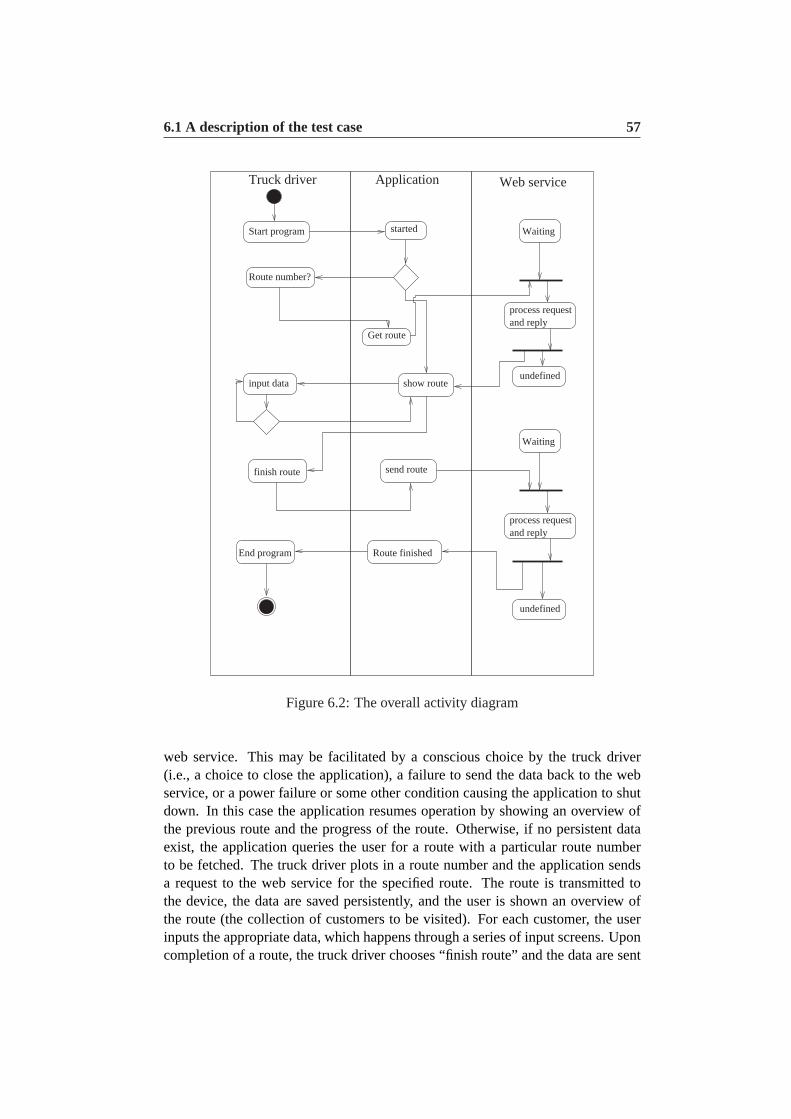
6.1 A description of the test case 57
Start program
Route number?
Get route
finish route
started
input data
End program
send route
show route
Route finished
process requestand reply
undefined
Waiting
process requestand reply
undefined
Waiting
Truck driver Web serviceApplication
Figure 6.2: The overall activity diagram
web service. This may be facilitated by a conscious choice by the truck driver(i.e., a choice to close the application), a failure to send the data back to the webservice, or a power failure or some other condition causing the application to shutdown. In this case the application resumes operation by showing an overview ofthe previous route and the progress of the route. Otherwise, if no persistent dataexist, the application queries the user for a route with a particular route numberto be fetched. The truck driver plots in a route number and the application sendsa request to the web service for the specified route. The route is transmitted tothe device, the data are saved persistently, and the user is shown an overview ofthe route (the collection of customers to be visited). For each customer, the userinputs the appropriate data, which happens through a series of input screens. Uponcompletion of a route, the truck driver chooses “finish route” and the data are sent
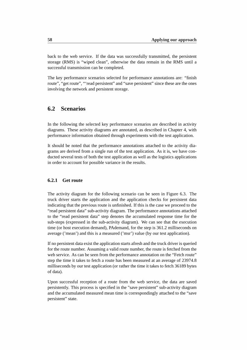
58 Applying our approach
back to the web service. If the data was successfully transmitted, the persistentstorage (RMS) is “wiped clean”, otherwise the data remain in the RMS until asuccessful transmission can be completed.
The key performance scenarios selected for performance annotations are: “finishroute”, “get route”, “‘read persistent” and “save persistent” since these are the onesinvolving the network and persistent storage.
6.2 Scenarios
In the following the selected key performance scenarios are described in activitydiagrams. These activity diagrams are annotated, as described in Chapter 4, withperformance information obtained through experiments with the test application.
It should be noted that the performance annotations attached to the activity dia-grams are derived from a single run of the test application. As it is, we have con-ducted several tests of both the test application as well as the logistics applicationsin order to account for possible variance in the results.
6.2.1 Get route
The activity diagram for the following scenario can be seen in Figure 6.3. Thetruck driver starts the application and the application checks for persistent dataindicating that the previous route is unfinished. If this is the case we proceed to the“read persistent data” sub-activity diagram. The performance annotations attachedto the “read persistent data” step denotes the accumulated response time for thesub-steps (expressed in the sub-activity diagram). We can see that the executiontime (or host execution demand), PAdemand, for the step is 361.2 milliseconds onaverage (’mean’) and this is a measured (’msr’) value (by our test application).
If no persistent data exist the application starts afresh and the truck driver is queriedfor the route number. Assuming a valid route number, the route is fetched from theweb service. As can be seen from the performance annotation on the “Fetch route”step the time it takes to fetch a route has been measured at an average of 23974.8milliseconds by our test application (or rather the time it takes to fetch 36189 bytesof data).
Upon successful reception of a route from the web service, the data are savedpersistently. This process is specified in the "save persistent” sub-activity diagramand the accumulated measured mean time is correspondingly attached to the “savepersistent” state.
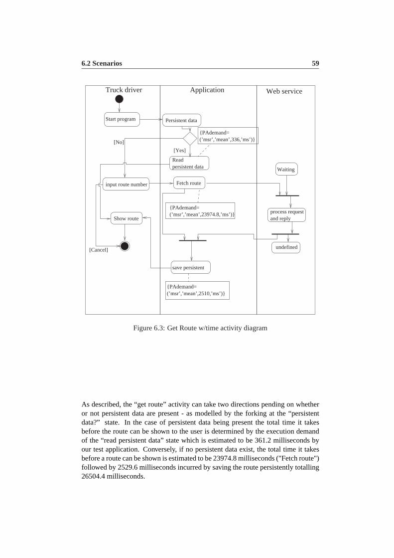
6.2 Scenarios 59
Start program
Readpersistent data
input route number Fetch route
save persistent
Show route
Truck driver Web service
process requestand reply
undefined
Waiting
Persistent data
{PAdemand=(’msr’,’mean’,23974.8,’ms’)}
{PAdemand=(’msr’,’mean’,2510,’ms’)}
{PAdemand=(’msr’,’mean’,336,’ms’)}
[Yes]
[No]
Application
[Cancel]
Figure 6.3: Get Route w/time activity diagram
As described, the “get route” activity can take two directions pending on whetheror not persistent data are present - as modelled by the forking at the “persistentdata?” state. In the case of persistent data being present the total time it takesbefore the route can be shown to the user is determined by the execution demandof the “read persistent data” state which is estimated to be 361.2 milliseconds byour test application. Conversely, if no persistent data exist, the total time it takesbefore a route can be shown is estimated to be 23974.8 milliseconds ("Fetch route")followed by 2529.6 milliseconds incurred by saving the route persistently totalling26504.4 milliseconds.
60 Applying our approach
save element
Open persistent storage
close persistent storage
{PAdemand=(’msr’,’mean’,150,’ms’)}
{PAdemand=(’msr’,’mean’,47.2,’ms’)
PArep=50}
{PAdemand=
(’msr’,’mean’,0,’ms’)}
[More elements]
[No more elemnts]
Application
Figure 6.4: Save persistent w/time activity diagram
6.2.2 Save persistent
Saving data in most cases is a three step process consisting of the steps of openinga record store, saving records to the record store, and closing the record store uponcompletion. Alternatively, a static reference to an open record store can be kept inwhich case the opening and closing of a record store are omitted from this process.As can be seen from the activity diagram in figure 6.4 we are modelling the firstcase. The average measured time to open a record store is derived from the resultsof running our test application and the "open persistent storage" step is annotatedwith this information.
The average time to write a record (save an element) is measured at 47.2 mil-liseconds and the number of elements to be saved in this example is 50 which isindicated by setting PArep (the repetition factor) to 50.

6.2 Scenarios 61
Thirdly, the appropriate average measured value is attached to the "close persistentstorage" step.
These three steps happen in succession and the total execution time for writing 50records (including opening and closing the record store) is thus 150 + (47.2 * 50)+ 0 = 2510 which, as we saw in the "get route" activity diagram, is the value givento the state encompassing this sub-activity.
6.2.3 Read persistent
Open persistent storage
close persistent storage
load element
{PAdemand=(’msr’,’mean’,6,’ms’)}
{PAdemand=(’msr’,’mean’,6.6,’ms’)PArep=50}
(’msr’,’mean’,0,’ms’)}{PAdemand=
[More elements]
[No more elemnts]
Application
Figure 6.5: Read persistent w/time activity diagram
Reading data from the RMS, illustrated in Figure 6.5, follow a path similar tothat of writing to the RMS. More specifically, it consists of the steps of opening arecord store, performing the reads (i.e., iterating over the record store and readingthe records) and closing the record store. As before, the steps are annotated withthe appropriate performance information obtained from running the test applicationand the resulting execution time for reading 50 elements from the RMS in this case
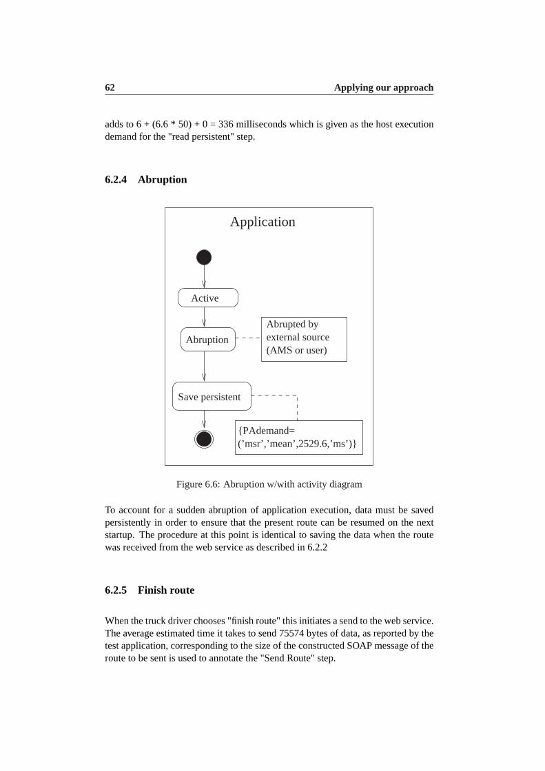
62 Applying our approach
adds to 6 + (6.6 * 50) + 0 = 336 milliseconds which is given as the host executiondemand for the "read persistent" step.
6.2.4 Abruption
Active
Save persistent
Abrupted by external source(AMS or user)
{PAdemand=(’msr’,’mean’,2529.6,’ms’)}
Abruption
Application
Figure 6.6: Abruption w/with activity diagram
To account for a sudden abruption of application execution, data must be savedpersistently in order to ensure that the present route can be resumed on the nextstartup. The procedure at this point is identical to saving the data when the routewas received from the web service as described in 6.2.2
6.2.5 Finish route
When the truck driver chooses "finish route" this initiates a send to the web service.The average estimated time it takes to send 75574 bytes of data, as reported by thetest application, corresponding to the size of the constructed SOAP message of theroute to be sent is used to annotate the "Send Route" step.
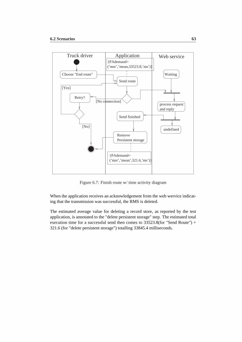
6.2 Scenarios 63
Choose "End route"
Retry?
Persistent storageRemove
Send finished
Send route
process requestand reply
undefined
Waiting
{PAdemand=(’msr’,’mean’,321.6,’ms’)}
{PAdemand=(’msr’,’mean,33523.8,’ms’)}
Truck driver Application
[Yes]
[No]
[No connection]
Web service
Figure 6.7: Finish route w/ time activity diagram
When the application receives an acknowledgement from the web wervice indicat-ing that the transmission was successful, the RMS is deleted.
The estimated average value for deleting a record store, as reported by the testapplication, is annotated to the "delete persistent storage" step. The estimated totalexecution time for a successful send then comes to 33523.8(for "Send Route") +321.6 (for "delete persistent storage") totalling 33845.4 milliseconds.

7Evaluatingour approach
In this chapter we investigate the extent to which our objective of creating an ap-proach that is useable, reliable, transparent, and cost-efficient are met. The bulkof the chapter is devoted to an investigation on the accuracy of the input estimatessupplied by the test application.
We present, compare and investigate the results obtained by running the test ap-plication and test case (logistics application) ten times each. The tests have beenconducted ten times each in order to account for variance in the results. The resultswe use for comparison are taken as the average of the ten tests. For the logistics ap-plication we have measured the best-case, worst-case, and average case scenarios.For instance, this means that the worst-case value we will use is the value obtainedby taking the average value of all the worst-case values and similarly for the thebest- and average cases.
The results from running the test application are delivered as three statistical mea-sures: the average, maximum and 95th percentile results. These are used to mea-sure the times ofsingleoperations (e.g., the time it takes to open a single recordstore or the time it takes to read a single record from a record store). In addition,the test application also return the total elapsed time for reading and writing all theelements of a record store. As with the results for the logistics application we usethe average value obtained over the course of the ten runs. In essence, we take theaverage of the ten maximum times, average times, and 95th percentile times.
According to Daniel A. Menascé, ACM Fellow, an error margin of up to 30% isconsidered acceptable in performance analysis [40]. We will investigate whether
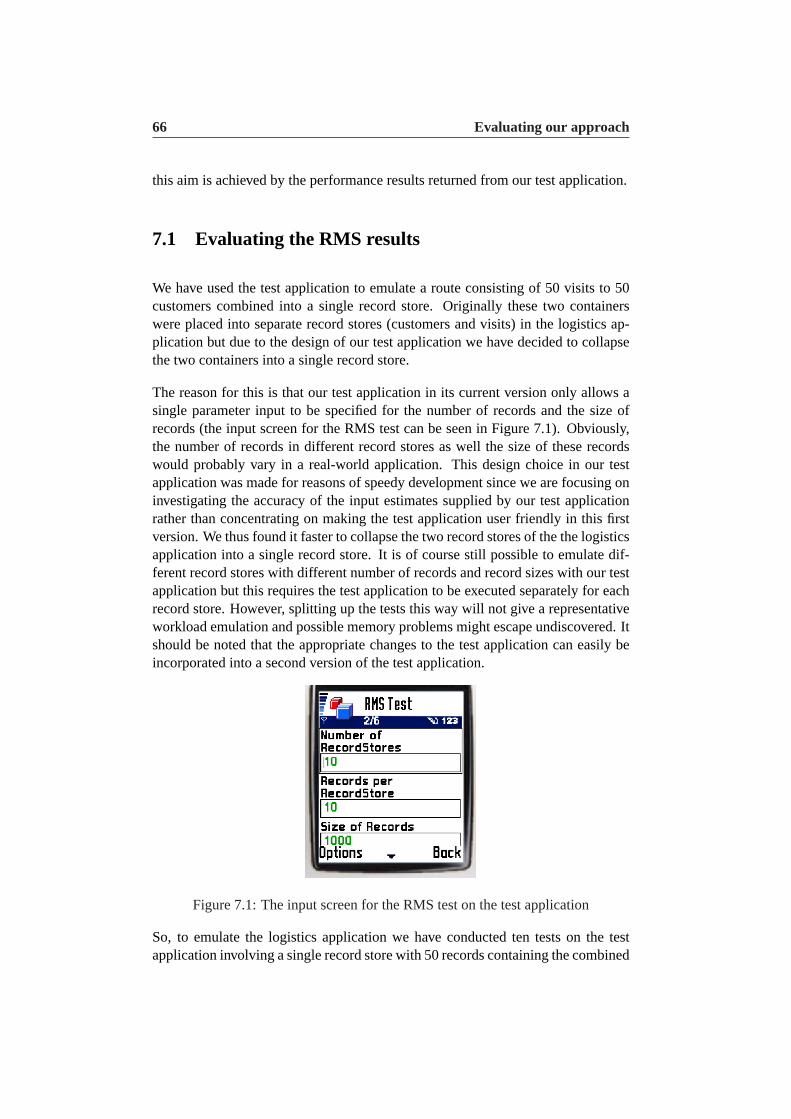
66 Evaluating our approach
this aim is achieved by the performance results returned from our test application.
7.1 Evaluating the RMS results
We have used the test application to emulate a route consisting of 50 visits to 50customers combined into a single record store. Originally these two containerswere placed into separate record stores (customers and visits) in the logistics ap-plication but due to the design of our test application we have decided to collapsethe two containers into a single record store.
The reason for this is that our test application in its current version only allows asingle parameter input to be specified for the number of records and the size ofrecords (the input screen for the RMS test can be seen in Figure 7.1). Obviously,the number of records in different record stores as well the size of these recordswould probably vary in a real-world application. This design choice in our testapplication was made for reasons of speedy development since we are focusing oninvestigating the accuracy of the input estimates supplied by our test applicationrather than concentrating on making the test application user friendly in this firstversion. We thus found it faster to collapse the two record stores of the the logisticsapplication into a single record store. It is of course still possible to emulate dif-ferent record stores with different number of records and record sizes with our testapplication but this requires the test application to be executed separately for eachrecord store. However, splitting up the tests this way will not give a representativeworkload emulation and possible memory problems might escape undiscovered. Itshould be noted that the appropriate changes to the test application can easily beincorporated into a second version of the test application.
Figure 7.1: The input screen for the RMS test on the test application
So, to emulate the logistics application we have conducted ten tests on the testapplication involving a single record store with 50 records containing the combined

7.1 Evaluating the RMS results 67
data of customers and visits. The size of the records come to a total of 637 bytes ((4× 150 for Strings) + (9× 4 for ints) + (1 for boolean) according to our assumptionof serialized strings occupying 150 bytes. The class diagram for a route can beseen in Figure 7.1.
Customer
public StringCustomername;public String Customernumberpublic int RMSIndex
Visit
public String CustomerOrdernumber;public String ordernumber;public int visitnumber;public int arrivalTime;public int returnBox;public int returnPallet;public int returnhalfPallet;public int box;public int pallet;public int halfPallet;public boolean visited=false;
11
Figure 7.2: The class diagram for the route
Table 7.1 shows the results of the logistics application specified as the average ofthe average, minimum (best case) and maximum (worst case) total times measuredin milliseconds for reading, writing and deleting 50 records over the course of tenruns.
Test avg. total time max. total time min. total timeReading 240,5 ms. 406 ms. 186 ms.Writing 3671,8 ms. 3812 ms. 3548 ms.Deleting 999,8 ms. 1047 ms. 953 ms.
Table 7.1: Results of RMS operations on the logistics application
Table 7.2 shows the results of our test application emulating the logistics applica-tion on ten different runs.
Test avg. max 95th percentile totalCreate 126,7 ms. 234 ms. 141 ms. –Open 3 ms. 15 ms. 15 ms. –Close 0 ms. 0 ms. 0 ms. –Read 6,9 ms. 50,2 ms. 16 ms. 372,1 ms.Write 47,7 ms. 135,9 ms. 96,8 ms. 2481,3 ms.Delete 323,3 ms. 344 ms. 343 ms. –
Table 7.2: The results returned from the test application emulating the workload ofthe logistics application
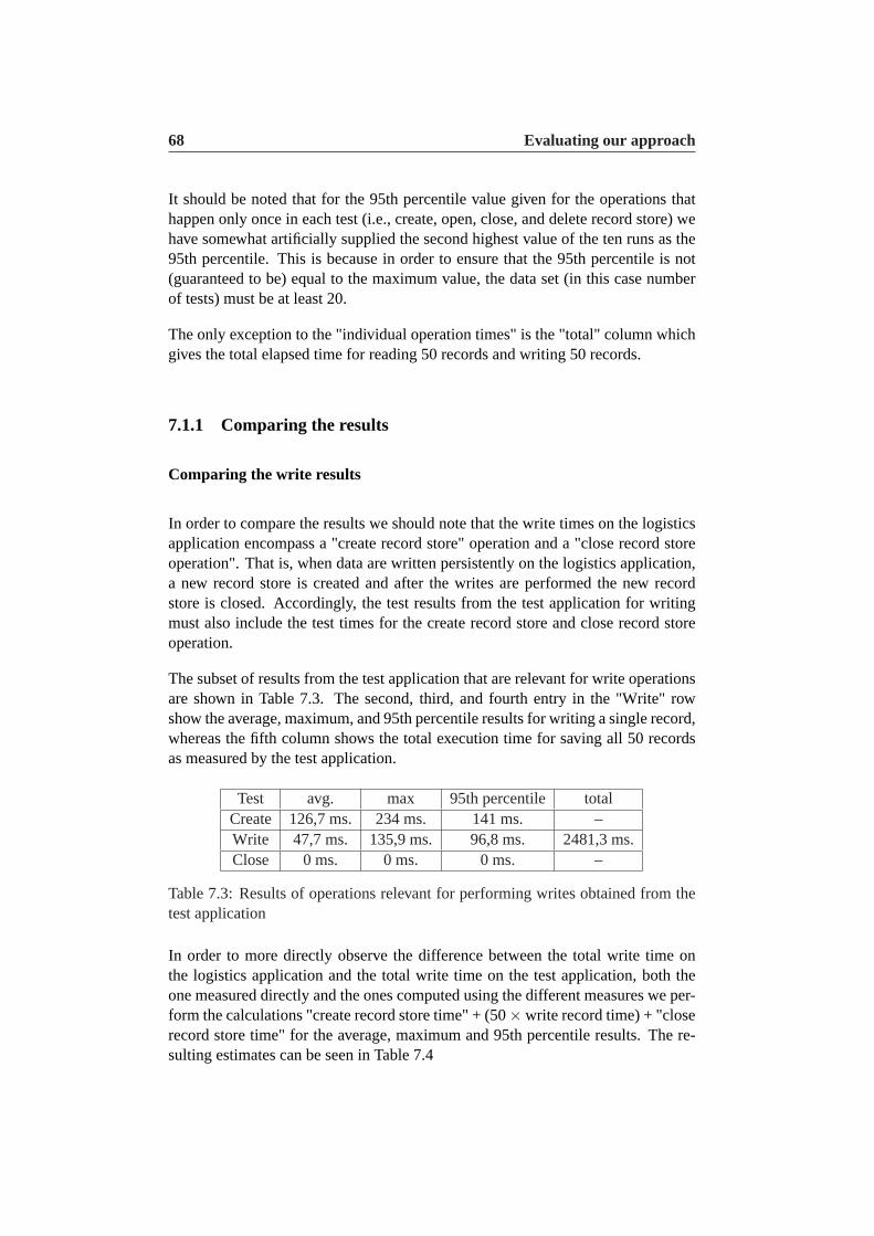
68 Evaluating our approach
It should be noted that for the 95th percentile value given for the operations thathappen only once in each test (i.e., create, open, close, and delete record store) wehave somewhat artificially supplied the second highest value of the ten runs as the95th percentile. This is because in order to ensure that the 95th percentile is not(guaranteed to be) equal to the maximum value, the data set (in this case numberof tests) must be at least 20.
The only exception to the "individual operation times" is the "total" column whichgives the total elapsed time for reading 50 records and writing 50 records.
7.1.1 Comparing the results
Comparing the write results
In order to compare the results we should note that the write times on the logisticsapplication encompass a "create record store" operation and a "close record storeoperation". That is, when data are written persistently on the logistics application,a new record store is created and after the writes are performed the new recordstore is closed. Accordingly, the test results from the test application for writingmust also include the test times for the create record store and close record storeoperation.
The subset of results from the test application that are relevant for write operationsare shown in Table 7.3. The second, third, and fourth entry in the "Write" rowshow the average, maximum, and 95th percentile results for writing a single record,whereas the fifth column shows the total execution time for saving all 50 recordsas measured by the test application.
Test avg. max 95th percentile totalCreate 126,7 ms. 234 ms. 141 ms. –Write 47,7 ms. 135,9 ms. 96,8 ms. 2481,3 ms.Close 0 ms. 0 ms. 0 ms. –
Table 7.3: Results of operations relevant for performing writes obtained from thetest application
In order to more directly observe the difference between the total write time onthe logistics application and the total write time on the test application, both theone measured directly and the ones computed using the different measures we per-form the calculations "create record store time" + (50×write record time) + "closerecord store time" for the average, maximum and 95th percentile results. The re-sulting estimates can be seen in Table 7.4
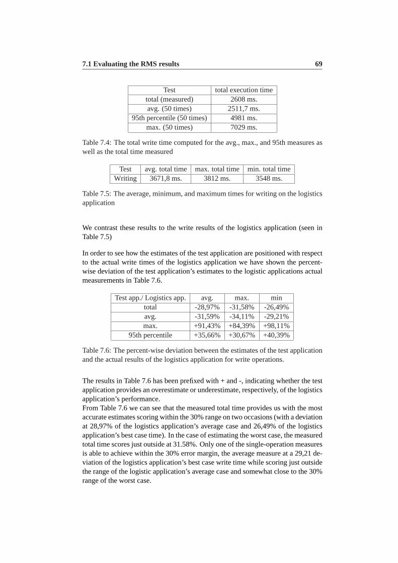
7.1 Evaluating the RMS results 69
Test total execution timetotal (measured) 2608 ms.avg. (50 times) 2511,7 ms.
95th percentile (50 times) 4981 ms.max. (50 times) 7029 ms.
Table 7.4: The total write time computed for the avg., max., and 95th measures aswell as the total time measured
Test avg. total time max. total time min. total timeWriting 3671,8 ms. 3812 ms. 3548 ms.
Table 7.5: The average, minimum, and maximum times for writing on the logisticsapplication
We contrast these results to the write results of the logistics application (seen inTable 7.5)
In order to see how the estimates of the test application are positioned with respectto the actual write times of the logistics application we have shown the percent-wise deviation of the test application’s estimates to the logistic applications actualmeasurements in Table 7.6.
Test app./ Logistics app. avg. max. mintotal -28,97% -31,58% -26,49%avg. -31,59% -34,11% -29,21%max. +91,43% +84,39% +98,11%
95th percentile +35,66% +30,67% +40,39%
Table 7.6: The percent-wise deviation between the estimates of the test applicationand the actual results of the logistics application for write operations.
The results in Table 7.6 has been prefixed with + and -, indicating whether the testapplication provides an overestimate or underestimate, respectively, of the logisticsapplication’s performance.From Table 7.6 we can see that the measured total time provides us with the mostaccurate estimates scoring within the 30% range on two occasions (with a deviationat 28,97% of the logistics application’s average case and 26,49% of the logisticsapplication’s best case time). In the case of estimating the worst case, the measuredtotal time scores just outside at 31.58%. Only one of the single-operation measuresis able to achieve within the 30% error margin, the average measure at a 29,21 de-viation of the logistics application’s best case write time while scoring just outsidethe range of the logistic application’s average case and somewhat close to the 30%range of the worst case.

70 Evaluating our approach
We can see that the maximum estimated time from the test application is of littleusage in estimating the performance of the logistics application. This is not sur-prising, as this is the estimate arrived at by taking the single longest write time andcompounding the effect of this by assuming that all records take this time to com-plete. We have observed quite a significant difference between the average caseand the occasional spike in write time incurred by the garbage collector (presum-ably) so this result could be expected. The reason for including it was to provide aworst case estimate.
The 95th percentile measure scores slightly worse than the average measure (in twoout of three cases). Only in the case of estimating the worst case performance of thelogistics application is the 95th percentile more accurate. Our primary concern ingeneral are the average and worst case performance that we can expect to achievefrom an application, and in the latter case the 95th percentile measure yields themore accurate estimate, just outside the 30% range (at 30,67%) thus giving the bestworst case estimate. An added benefit of the 95th percentile is that it errs on theright side of caution so to speak, in that it does not give underestimates of the actualperformance.
Comparing the read results
As for writes, reads also incur two additional operations. In this case an "openrecord store" operation as well as a "close record store" operation.
We show the results of the read-relevant operations from the test application inTable 7.7
Test avg. max 95th percentile totalOpen 3 ms. 15 ms. 15 ms. –Read 6,9 ms. 50,2 ms. 16 ms. 372,1 ms.Close 0 ms. 0 ms. 0 ms. –
Table 7.7: Results of operations relevant for performing reads obtained from thetest application
Also, to get a clearer picture of the differences between the estimates suppliedby using the different measures we give their resulting estimates ("time of openrecord store operation" + "50× "individual read operations" + "close record storeoperation". These results can be seen in Table 7.8
We recap the read times from the logistics application in Table 7.9
We then show the accuracy of the read predictions from the test application inrelation to their percent-wise deviation from the actual read results measured on
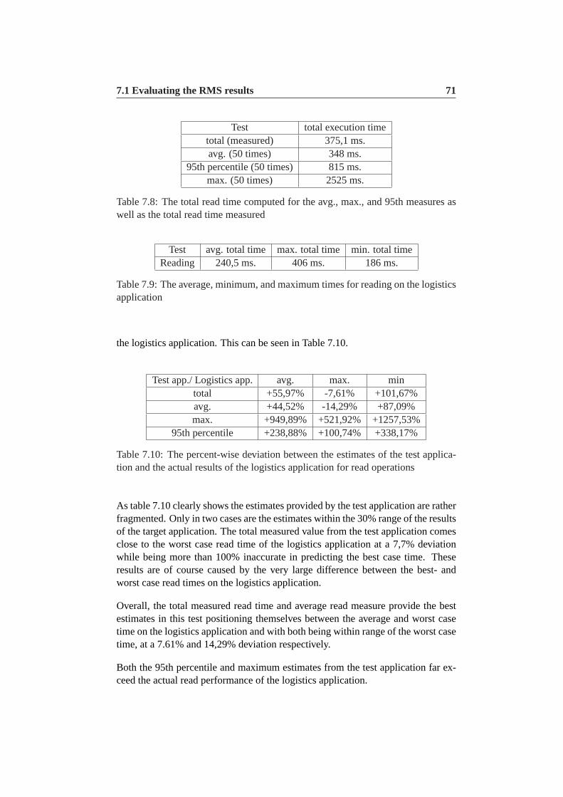
7.1 Evaluating the RMS results 71
Test total execution timetotal (measured) 375,1 ms.avg. (50 times) 348 ms.
95th percentile (50 times) 815 ms.max. (50 times) 2525 ms.
Table 7.8: The total read time computed for the avg., max., and 95th measures aswell as the total read time measured
Test avg. total time max. total time min. total timeReading 240,5 ms. 406 ms. 186 ms.
Table 7.9: The average, minimum, and maximum times for reading on the logisticsapplication
the logistics application. This can be seen in Table 7.10.
Test app./ Logistics app. avg. max. mintotal +55,97% -7,61% +101,67%avg. +44,52% -14,29% +87,09%max. +949,89% +521,92% +1257,53%
95th percentile +238,88% +100,74% +338,17%
Table 7.10: The percent-wise deviation between the estimates of the test applica-tion and the actual results of the logistics application for read operations
As table 7.10 clearly shows the estimates provided by the test application are ratherfragmented. Only in two cases are the estimates within the 30% range of the resultsof the target application. The total measured value from the test application comesclose to the worst case read time of the logistics application at a 7,7% deviationwhile being more than 100% inaccurate in predicting the best case time. Theseresults are of course caused by the very large difference between the best- andworst case read times on the logistics application.
Overall, the total measured read time and average read measure provide the bestestimates in this test positioning themselves between the average and worst casetime on the logistics application and with both being within range of the worst casetime, at a 7.61% and 14,29% deviation respectively.
Both the 95th percentile and maximum estimates from the test application far ex-ceed the actual read performance of the logistics application.
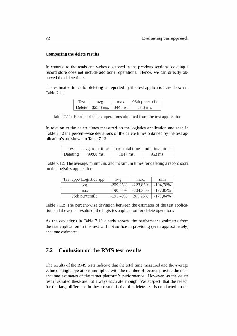
72 Evaluating our approach
Comparing the delete results
In contrast to the reads and writes discussed in the previous sections, deleting arecord store does not include additional operations. Hence, we can directly ob-served the delete times.
The estimated times for deleting as reported by the test application are shown inTable 7.11
Test avg. max 95th percentileDelete 323,3 ms. 344 ms. 343 ms.
Table 7.11: Results of delete operations obtained from the test application
In relation to the delete times measured on the logistics application and seen inTable 7.12 the percent-wise deviations of the delete times obtained by the test ap-plication’s are shown in Table 7.13
Test avg. total time max. total time min. total timeDeleting 999,8 ms. 1047 ms. 953 ms.
Table 7.12: The average, minimum, and maximum times for deleting a record storeon the logistics application
Test app./ Logistics app. avg. max. minavg. -209,25% -223,85% -194,78%max -190,64% -204,36% -177,03%
95th percentile -191,49% 205,25% -177,84%
Table 7.13: The percent-wise deviation between the estimates of the test applica-tion and the actual results of the logistics application for delete operations
As the deviations in Table 7.13 clearly shows, the performance estimates fromthe test application in this test will not suffice in providing (even approximately)accurate estimates.
7.2 Conlusion on the RMS test results
The results of the RMS tests indicate that the total time measured and the averagevalue of single operations multiplied with the number of records provide the mostaccurate estimates of the target platform’s performance. However, as the deletetest illustrated these are not always accurate enough. We suspect, that the reasonfor the large difference in these results is that the delete test is conducted on the

7.3 Evaluating the network results 73
logistics application at a time when the garbage collector is reclaiming objectswhereas the test application conducts a "clean" RMS test meaning no additionalobjects are created and destroyed. The garbage collector may be the cause of theanomalies in the estimates. One way to investigate this would be to force a garbagecollection on the target application (for validation purposes) and see whether theperformance estimates of the test application and the performance of the logisticsapplication would then be approximately similar. (However, as we were sharingthe Nokia phone with another project group also working on their master thesis wewere not able to try out this possibility in time.) If indeed the garbage collectorproved to be the cause of the anomaly it would be beneficial to try and apply ourtest application to additional target applications of varying complexities in order toinvestigate this effect.
Performance on the target application may also vary significantly between indi-vidual runs, as we saw from the results in the read test. This, of course, makesit difficult to provide accurate estimates in every single run and also illustrate thegeneral problem of providing accurate performance predictions of object-orientedsystems.
7.3 Evaluating the network results
We have conducted five runs of the test application where we emulated fetching36189 bytes data which contains information about which customers the drivershall visit on his route. We also emulated sending the route back when the day isover and the size of this data is 75574 bytes. When sending back the route moreinformation is sent, e.g. what packaging items have been dropped of and whatpackaging items has been returned, which is the cause of the larger byte size tosend than receive.
Test avg. time max time min timeGet route 28549,8 29297 28141Send route 39240,2 39953 38484
Table 7.14: Results of Networking operations in the logistics application
The results given in Table 7.14 is for the logistics application. The “get route”times include the time it takes to accept the network connection and to chose aconnection profile, and the “send route” include the time it takes to accept thenetwork connection.
The results from the test application are given as the average, maximum, and 95thpercentile, and the same issue regarding acceptance of network connection andconnection profile also applies to the test application.
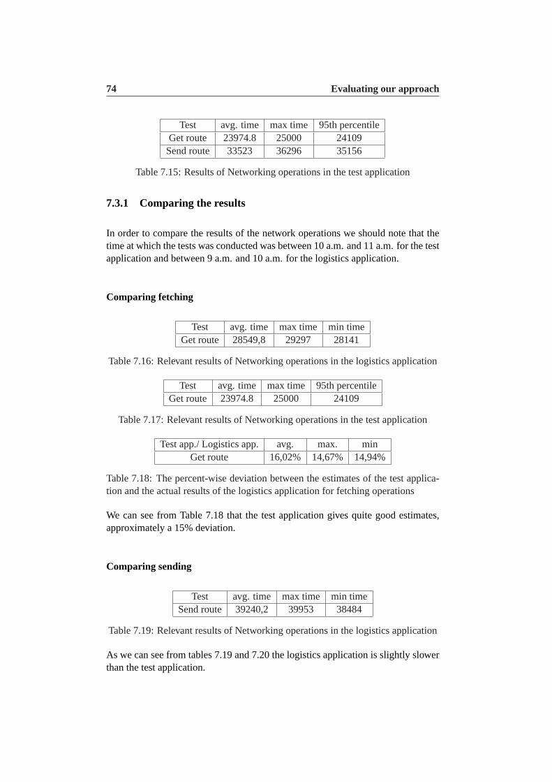
74 Evaluating our approach
Test avg. time max time 95th percentileGet route 23974.8 25000 24109Send route 33523 36296 35156
Table 7.15: Results of Networking operations in the test application
7.3.1 Comparing the results
In order to compare the results of the network operations we should note that thetime at which the tests was conducted was between 10 a.m. and 11 a.m. for the testapplication and between 9 a.m. and 10 a.m. for the logistics application.
Comparing fetching
Test avg. time max time min timeGet route 28549,8 29297 28141
Table 7.16: Relevant results of Networking operations in the logistics application
Test avg. time max time 95th percentileGet route 23974.8 25000 24109
Table 7.17: Relevant results of Networking operations in the test application
Test app./ Logistics app. avg. max. minGet route 16,02% 14,67% 14,94%
Table 7.18: The percent-wise deviation between the estimates of the test applica-tion and the actual results of the logistics application for fetching operations
We can see from Table 7.18 that the test application gives quite good estimates,approximately a 15% deviation.
Comparing sending
Test avg. time max time min timeSend route 39240,2 39953 38484
Table 7.19: Relevant results of Networking operations in the logistics application
As we can see from tables 7.19 and 7.20 the logistics application is slightly slowerthan the test application.
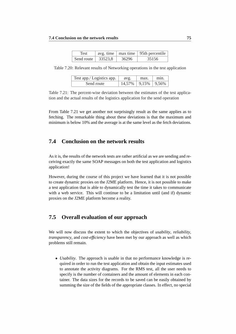
7.4 Conclusion on the network results 75
Test avg. time max time 95th percentileSend route 33523,8 36296 35156
Table 7.20: Relevant results of Networking operations in the test application
Test app./ Logistics app. avg. max. min.Send route 14,57% 9,15% 9,56%
Table 7.21: The percent-wise deviation between the estimates of the test applica-tion and the actual results of the logistics application for the send operation
From Table 7.21 we get another not surprisingly result as the same applies as tofetching. The remarkable thing about these deviations is that the maximum andminimum is below 10% and the average is at the same level as the fetch deviations.
7.4 Conclusion on the network results
As it is, the results of the network tests are rather artificial as we are sending and re-ceiving exactly the same SOAP messages on both the test application and logisticsapplication!
However, during the course of this project we have learned that it is not possibleto create dynamic proxies on the J2ME platform. Hence, it is not possible to makea test application that is able to dynamically test the time it takes to communicatewith a web service. This will continue to be a limitation until (and if) dynamicproxies on the J2ME platform become a reality.
7.5 Overall evaluation of our approach
We will now discuss the extent to which the objectives ofusability, reliability,transparency, andcost-efficiencyhave been met by our approach as well as whichproblems still remain.
• Usability. The approach is usable in that no performance knowledge is re-quired in order to run the test application and obtain the input estimates usedto annotate the activity diagrams. For the RMS test, all the user needs tospecify is the number of containers and the amount of elements in each con-tainer. The data sizes for the records to be saved can be easily obtained bysumming the size of the fields of the appropriate classes. In effect, no special
76 Evaluating our approach
performance knowledge is required to conduct the tests and achieve the in-put estimates. The annotation of activity diagrams is conducted as part of thedesign of the system which means that performance evaluation is effectivelyfused into the design process rather than being a separate activity. By makingperformance evaluation an intrinsic part of the design process we also ensurethat the performance estimates are always accurate reflections of the currentstate of the design, hereby removing the concern of having to keep a separateperformance modeling effort up to par with the evolving design. An addedbenefit of our test application is that it implicitly conducts a feasibility studyof the system to be built - if the test application throws an OutOfMemoryexception with the specified parameters, then certainly the target applicationis very much at risk of doing so also, as the test application is stripped ofexcess functionality. Developers can then use this information to consideran alternative design.
• Reliabilityof estimates. We have seen that the estimates of our approach arefairly accurate in the majority of instances when using the total measuredtime and average individual time as measures. However, in the RMS test weobserved that in a single test (delete record store) the estimates were not validpredictions. We attributed this effect to the garbage collector reclaimingobjects during the deletion of record stores on the logistics application butwe will have to conduct additional tests on other applications, varying fromvery simple applications to more complex applications, to investigate theimpact of the garbage collector further.
• Transparency. We have not been able to fully achieve the transparencyobjective in practice. Instead in our current effort we have relied on anad-hoc approach to performance modelling using the algorithm for trans-forming sequence diagrams to execution graphs which can also be appliedto activity diagrams. The reason that we are saying "not fully" is that thetransformation algorithm is straight-forward to apply and as such does notrequire knowledge of execution graphs and can thus be performed by non-specialists. However it is not optimal from a transparency viewpoint. Ideally,the construction and solution of an appropriate performance model shouldbe completely hidden from the developer. The UML-SPT profile lends itselftowards integration with performance tools by the transformation processdescribed in Chapter 4. As a result, we expect performance tools to inte-grate more closely with UML tools in the future. As the UML-SPT profileis still rather new (it went into final release on January 2005) no UML toolsyet support the performance component of the profile. Also, presently theredoes not seem to exist a performance tool that, without any intervention froma developer, can take an XML representation of an activity diagram, com-pute a performance prediction, and report it back into an XML representationthat could be imported by a UML modelling tool. Thus, achieving full trans-
7.5 Overall evaluation of our approach 77
parency is not yet possible by use of existing UML and performance tools.
• Cost-efficiency. Our approach is cheap to realize. It incurs an initial modestlearning curve associated with familiarizing developers with the UML-SPTprofile (and with the activity diagram-to-execution graph algorithm in ourcurrent installment to compute the result estimates). Otherwise, using ourapproach is as simple (and cheap) as executing the test application to assim-ilate the input estimates and annotating the input estimates to the activitydiagrams.
As we have noted, since dynamic proxies are not a reality on the J2ME platform,our test application at the present time is not applicable to web services. This limi-tation can only be resolved once (and indeed if) dynamic proxies become availableon the J2ME platform.


Part III
Conclusion and future work

8Conclusion
Performance can be a make or break factor in determining the success of softwareprojects. Examples to this fact follows:
NASA was forced to delay the launch of a satellite for a least eight months dueto the Flight Operation Segment (FOS) software in the satellite having unaccept-able response times for developing satelitte schedules and poor performance inanalyzing satellite status and telemetry data. The cost of the delay has not beendetermined, but there is certainly a loss of prestige, and members of Congressquestioned NASA’s ability to manage the program. [41]
Similar problems have been experienced in the B2C market.
“In 2001 $25 billion were lost due to web performance issues” (ZonaResearch) [32]
“48% of online shoppers gave up trying to buy some products onlinebecause web pages took too long to load” (Boston Consulting) [32]
And finally, a domestic example: In what has been dubbed the largest scandal inDanish computer software history, The Amanda system - a system to to aid theDanish public servant caseworkers in handling cases faster and more efficiently -failed miserably in a national stress test by showing response times upwards of anhour and a half. Although the system exhibited a multitude of additional problems[10], these response times by themselves clearly made the system useless.
A common misconception is that Moore’s Law has rendered performance con-siderations superfluous. However, this is far from the case as evidenced by the
82 Conclusion
substantial investments being made in performance management. In 1998 the per-formance management market stood at about 2 billion dollars - by 2005 this num-ber has grown to just over 4.5 billion dollars [32]. This increase clearly showsthat waiting 18 months for Moore’s law to take effect simply is not an option in acompetitive market.
Despite the importance of performance, performance considerations in traditionalsoftware engineering have been subject to a fix-it-later attitude although correctingperformance at a late stage in the development process can be extremely costly andin some cases impossible. Moreover, targeting performance by means of perfor-mance tuning and optimizations may erode other software quality attributes suchas the maintainability and flexibility of the system.
Software Performance Engineering (SPE) tries to address this shortcoming by con-sidering performance early in the development process.
So far, SPE has not been incorporated into the mainstream software engineering(SE) discipline which is underlined by the fact that SPE is indeed still a separatediscipline.
A fundamental reason for this may be that performance-related subjects are scarcelybeing taught at the majority of computer science schools - often performance ismentioned as a side note, and often performance is inadequately or not defined.The problem is worsened when it comes to knowledge of SPE - a survey [21]showed that out of 24 highly ranked computer science schools in the United Statesonly two courses mentioned SPE, and one of these even incorrectly implied thatSPE was a specialized discipline for database-centered and real-time applications.
This has made the adoption of SPE into a software development effort highly de-pendant upon specialized staff being available with an appropriate amount of per-formance skills and experience.
In this thesis we have pointed to a number of deficiencies of using such an ap-proach.
• The reliance on a performance specialist in order to be able to obtain per-formance estimates of the design of a system limits the usability of SPE inordinary software development projects.
• The reliability of the performance estimates of the system is dependent onthe level of expertise of the performance specialist who supplies the inputestimates.
• SPE is costly - it consists of an iterative process of performance model cre-ation and solution combined with validation and verification of the models inorder to obtain increasingly accurate reflections of the system’s performance.
83
We proposed an approach to making early performance evaluation significantlymore appealing to incorporation into traditional software development by 1) sub-stituting the input estimates supplied by a performance specialist with a test ap-plication that would provide these input estimates instead and 2) hiding details ofperformance model creation and solution to the developer as well as eradicatingthe need to posses intricate knowledge of the device characteristics of the devicesto be developed to.
The focus of our approach in this thesis has been directed at performance on theJ2ME platform where we have investigated performance concerns regarding thetwo areas that are notoriously “heavy hitters”: network usage and persistent stor-age. The motivation is that the effects of these two areas are felt particularly ondevices with limited capabilities such as is the case of wireless devices. We haveused an end-to-end application (J2ME-J2EE), which we have developed as part ofa previous project, as a test case in order to investigate the validity of our approach.
We came to the following conclusions regarding the usability, realibility, trans-parency and cost-efficiency of our approach:
Usability Our approach is usable to "ordinary" SE developers in that no specialperformance skills are required.
Reliability of estimates We conducted a number of tests of our test applicationas well of our test case application in order to determine whether the input estimatesprovided by the test application could be used as a basis for predicting the actualperformance of the test case application. We observed that the input estimatesfrom our test application in the majority of cases were able to provide reasonablyaccurate reflections of the performance of the test case. However, in a single test weobserved an anomali where the performance of the test case where several factorsworse than than the actual performance of the test case. Similarly, we noted that theperformance of the test case application in the RMS read test varied substantiallywith the worst case taking more than twice the time of the best case to complete.This contributes to making performance predictions in every single run of the testapplication reliable. We attributed these variations to the garbage collector.
Transparency Within the time frame of this thesis we have not been able toimplement a tool (possibly an add-in to an existing UML tool) that would be able tocompute the final performance predictions of a system based on the input estimatesfrom our test application. Also, no UML and performance tools exist that supportthe model processing process of of UML diagrams. Instead, we have relied on anad-hoc execution graph solution of the system.
84 Conclusion
Cost-efficiency The cost of our approach is negligible. It involves the cost to ex-ecute the test application, which can be done within a matter of a very few minutes,as well as the cost of annotating the activity diagrams with performance informa-tion, which is done as part of the design.
8.1 Shortcomings and future work
The test application at the present time is not applicable to web services. This isdue to the fact that the creation of dynamic proxies is not possbile on the J2MEplatform. However, instead of waiting for dynamic proxies to become a reality onthe J2ME platform, a future work may consider estimating the size of the SOAPmessages to be sent by investigating the WSDL file describing the web service.We could then time the operation of sending and receiving the computed amountof bytes. The network time could then be combined with a test of various XMLparsers to try and estimate the total time of using web services.
An immediate future work includes further tests to investigate the impact of garbagecollection. We could conduct additional tests of more applications, ranging fromsimple ones, where the number of objects are limited, to more complex applica-tions carrying a larger memory footprint. It would also be beneficial to conductthese tests on different devices that have different garbage collection implementa-tions.
Regarding the achievement of transparency, once the UML-SPT profile becomesincorporated into UML tools the automatization of the model processing processof UML diagrams will become realizable in practice.
A natural extension to the approach suggested in this thesis would be to includemore general performance considerations in J2ME applications, in particular in-vestigating the overhead of using object orientation in wireless devices.
Another direction may be to investigate our approach on other platforms, such asstandalone computers and enterprise applications where the heterogenity of bothhardware and software far exceeds that of the J2ME platform.
A limitation, not only of our approach but of performance engineering in general,is that timeliness is the only performance measure considered. An application’smemory consumption can be critical to its success. If the application uses exces-sive memory the garbage collector, which may be very primitive on many wirelessdevices, will have to free the allocated memory - a process which may have a sig-nificant impact on the overall performance, particularly on a wireless device.
8.2 Summary 85
8.2 Summary
Performance, or a lack thereof, can mean the difference between succes or failurein a software project. A lack of satisfactory performance may cause schedule andcost overruns and in some cases project cancellation. In a competitive market theperformance of a software product may in some cases be the determining factor indeciding which product to use. These are all compelling reasons to give the per-formance aspect a high priority in the design of a software system. The reality is,however, that performance has usually been relegated to the late life cycle stagesin traditional software engineering. The popular belief has been that possible per-formance problems can be solved through code optimization and tuning. However,such an approach has several flaws: Not only can performance problems incur con-siderable costs to fix at such a late stage, but fixing performance problems throughcode optimations and tuning may also very well impair other quality traits of thesystem, such as the maintainabilty and flexibility of the system, since the code ismade more complex and thus harder to understand. Finally, some performanceproblems are impossible to fix through code optimization and tuning - they reflectfaulty design choices that can only be corrected through extensive re-design of thesystem.
A discipline called “Software Performance Engineering (SPE)” emerged in theeighties with the aim of trying to adress performance issues at the design time ofsystems, and by including explicit performance considerations already in the analy-sis phase of a development process. However, SPE has never really caught on in themainstream software engineering practices. The reasons for this is that SPE relieson specialized formalisms for modelling the performance which are generally notbeing taught in the computer science courses at the majority of universities. Thismeans that the amount of people that have the necessary knowledge to conductSPE is limited, and SPE thus becomes inherently people-dependant.
In our master thesis we have proposed and investigated the validity of an approachthat tries to incorporate early performance evaluation into software engineeringwithout having to rely on specialized staff. The approach towards achieving thisobjective was to try and automate the process of obtaining input estimates whichwould otherwise have to be supplied by a performance specialist. The means fordoing so is a test application that we have created as part of this project that capturesperformance characteristics of a target device. The test application can be usedwithout any special performance knowledge to obtain input estimates. The inputestimates returned from the test application are used to annotate activity diagramswith performance information according to the UMLTM Profile for Schedulability,Performance, and Time(UML-SPT). The annotated activity diagrams are then usedto give a performance prediction of the system to be built.
86 Conclusion
Our work has concentrated on estimating performance for J2ME applications. Morespecifically we have targeted our effort on estimating performance for the two ar-eas on the J2ME platform that typically constitute the greatest performance bottle-necks: persistent storage and networking.
To validate our approach we have applied it to a test case. We conducted a num-ber of tests of our test application and test case to investigate whether the inputestimates from the test application could be used as a basis for predicting the ac-tual performance of the test case. The results from these tests showed that in themajority of cases this was fulfilled.
Our thesis is divided into three major parts:
In the first part of this thesis we investigated the existing work in the field ofSoftware Performance Engineering and analysed the shortcomings hindering theadoption of SPE into the mainstream Software Engineering practices. Next, wedescribed the performance relevant aspects of the UML-SPT profile in order toilluminate the concepts and extensions to the UML metamodel that allows for per-formance to be included in UML modeling.
We commenced the second part of the thesis with a description of our approach.We went on to illustrate how our approach is used as part of the design effort andthe part concluded with an evaluation of the extent to which our approach is usablefrom a Software Engineering standpoint.
Finally, in the third part of this thesis we concluded on our work and discussedpossible future work.
Bibliography
[1] Device specifications for nokia n70.http://www.forum.nokia.com/devices/N70 .
[2] Device specifications for nokia n90.http://www.forum.nokia.com/devices/N90 .
[3] Device specifications for nokia n91.http://www.forum.nokia.com/devices/N91 .
[4] K. Auer and K. Beck. Lazy optimization: Patterns for efficient smalltalkprogramming. In J. Vlissides, J. Coplien, and N. Kerth, editors,Pattern Lan-guages of Program Design, volume 2. Addison-Wesley, 1996.
[5] Doug Bell. Make java fast: Optimize! Internet:http://www.javaworld.com/javaworld/jw-04-1997/jw-04-optimize.html .
[6] Christina Catley, Dorina C. Petriu, and Monique Frize. Software performanceengineering of a web service-based clinical decision support infrastructure.In Proceedings of the fourth international workshop on Software and per-formance, pages 130–138. SIGMETRICS: ACM Special Interest Group onMeasurement and Evaluation and SIGSOFT: ACM Special Interest Group onSoftware Engineering, ACM Press, New York, NY, USA, 2004.
[7] Simul8 Corporation. Simul8. Internet:http://www.simul8.com/ .
[8] Vittorio Cortellessa and Raffaela Mirandola. Deriving a queueing networkbased performance model from uml diagrams.http://portal.acm.org/citation.cfm?id=350406 , 2000. SIGMETRICS: ACM SpecialInterest Group on Measurement and Evaluation and SIGSOFT: ACM SpecialInterest Group on Software Engineering, ACM Press, New York, NY, USA.
[9] Vittorio Cortellessa and Raffaela Mirandola. Prima-uml: a performance vali-dation incremental methodology on early uml diagrams.Science of ComputerProgramming, 44(1):101–129, 2002.
88 BIBLIOGRAPHY
[10] Stig Dahl. Problembarnet amanda. Internet:http://cph.ing.dk/arkiv/2400/amanda1.html , 2000.
[11] Gentleware. Poseidon for uml. Internet:http://www.gentleware.com/ .
[12] Eric Giguere. Record management system basics. Internet:http://developers.sun.com/techtopics/mobility/midp/ttips/rmsbasics/ , 2001.
[13] The OMG Group. Uml profile for schedulability, performance, and time spec-ification. January 2005.
[14] Gordon P. Gu and Dorina C. Petriu. Xslt transfor-mation from uml models to lqn performance models.http://portal.acm.org/citation.cfm?doid=584369.584402, 2002. SIGMET-RICS: ACM Special Interest Group on Measurement and Evaluation andSIGSOFT: ACM Special Interest Group on Software Engineering, ACMPress, New York, NY, USA.
[15] Gordon Ping Gu and Dorina C. Petriu. Early evaluation of software perfor-mance based on the uml performance profile. InProceedings of the 2003conference of the Centre for Advanced Studies on Collaborative research,2003.
[16] Stefan Haustein. Internet:http://www.ksoap.org .
[17] Stefan Haustein. Internet:http://www.kobjects.org .
[18] Jane Hillston. Pepa (performance evaluation process algebra). Internet:http://www.dcs.ed.ac.uk/pepa/ .
[19] IBM. Rational rose xde developer.http://www-306.ibm.com/software/awdtools/developer/rosexde/ .
[20] I. Jacobson, G. Booch, and J. Rumbaugh.The Unified Software DevelopmentProcess. Addison-Wesley, 1999.
[21] Robert F. Dugan Jr. Performance lies my professor told me: The case forteaching software performance engineering to undergraduates. InProceed-ings of the fourth international workshop on Software and performance. De-partment of Computer Science, Stonehill College, ACM Press, New York,NY, USA, 2004.
[22] David P. Kelly and Robert S. Oshana. Software performance engineeringa digital signal processing application.http://portal.acm.org/citation.cfm?id=287328&coll=Portal&dl=GUIDE&CFID=44134284&CFTOKEN=22262372, 1998. SIGMETRICS: ACM Special
BIBLIOGRAPHY 89
Interest Group on Measurement and Evaluation and SIGSOFT: ACM SpecialInterest Group on Software Engineering, ACM Press, New York, NY, USA.
[23] M. Litoiu, Hamid Khafagy, Bin Qin, Anita Rass Wan, and J. Rolia. A perfor-mance engineering tool and method for distributing applications. InProceed-ings of the 1997 conference of the Centre for Advanced Studies on Collabo-rative research. IBM Centre for Advanced Studies Conference, IBM Press,1997.
[24] Juan Pablo López-Grao, José Merseguer, and Javier Campos. From uml ac-tivity diagrams to stochastic petri nets: Application to software performanceengineering. http://portal.acm.org/citation.cfm?id=974048&coll=Portal&dl=GUIDE&CFID=44134284&CFTOKEN=22262372 , 2004. SIGMETRICS: ACM Special Interest Group on Mea-surement and Evaluation and SIGSOFT: ACM Special Interest Group onSoftware Engineering, ACM Press, New York, NY, USA.
[25] No magic Inc. Magic draw uml. Internet:http://www.magicdraw.com/ .
[26] Daniel A. Menascé and Hassan Gomaa. On a language basedmethod for software performance engineering of client/server systems.http://portal.acm.org/citation.cfm?id=287331&coll=Portal&dl=GUIDE&CFID=44134284&CFTOKEN=22262372 , 1998.SIGMETRICS: ACM Special Interest Group on Measurement and Evalua-tion and SIGSOFT: ACM Special Interest Group on Software Engineering,ACM Press, New York, NY, USA.
[27] Daniel A. Menascé. Software, performance, or engineering? InProceed-ings of the third international workshop on Software and performance. De-partment of Computer Science, George Mason University, ACM Press, NewYork, NY, USA, 2002.
[28] Ole Mertz, Kim Algreen, René Hansen, and Dennis Micheelsen..NET vs.Java - mobilklienter og web services. The Faculty of Enginerring and Science- Department of Computer Science, Fredrik Bajers vej 7, 9210 Aalborg SOE,2005.
[29] Visual Object Modelers. Visual uml. Internet:http://www.visualuml.com/ .
[30] Object Management Group, Inc, http://www.omg.org/technology/documents/formal/xmi.htm . XML MetadataInterchange (XMI).
[31] Object Management Group, Inc.(OMG),http://www.uml.org/ . UML2.0 Superstructure Specification, version 2.0 edition, October 2004.
90 BIBLIOGRAPHY
[32] Stathis Papaefstathiou. State of the art of performance capabilitesof commercial development environments. volume ACM WOSP2002,http://research.microsoft.com/~efp/WOSP%202002%20Tutorial.ppt , 2002. Microsoft, Redmond, USA.
[33] Visual Paradigm. Visual paradigm for uml (vp-uml). Internet:http://www.visual-paradigm.com/product/vpuml/ .
[34] University of Illinois at Urbana-Champaign PERFORM Performability En-gineering Research Group. Möbius. Internet:http://www.mobius.uiuc.edu/index.html .
[35] Dorina C. Petriu and Hui Shen. Applying the uml performance pro-file: Graph grammar-based derivation of lqn models from uml spec-ifications. Internet: http://www.sce.carleton.ca/faculty/petriu/papers/TOOLS2002.pdf , 2002.
[36] Roger S. Pressman.Software Engineering. A Practitioner’s Approach. AlfredWaller. McGraw-Hill International (UK) Limited, 2000.
[37] Stanislaw Raczynski. Qms: Queueing model simulation. Internet:http://www.raczynski.com/pn/qms.htm .
[38] Andreas Schmietendorf, Evgeni Dimitrov, and Reiner R. Dumke. Processmodels for the software development and performance engineering tasks.In Proceedings of the third international workshop on Software and perfor-mance. ACM Press, New York, NY, USA, 2002.
[39] Peter Sestoft. Java performance: Reducing time and space consumption.
[40] James Skene. Unobtrusive performance analysisU where is the qos intapas? Internet:http://www.cs.ucl.ac.uk/staff/j.skene/tapas/TAPAS-pres-2.ppt#1 .
[41] Connie U. Smith and Lloyd G. Williams.Performance Solutions: A Practi-cal Guide to Creating Responsive, Scalable Software. ADDISON-WESLEY,2002.
[42] Dr. Connie U. Smith. Spe-edTM . Internet:http://www.perfeng.com/sped.htm .
[43] Mesquite software. Csim. Internet:http://www.mesquite.com/ .
[44] Ian Sommerville.Software Engineering. Addison-Wesley and Pearson Edu-cation Limited, 6 edition, 2001.
[45] Unknown. Queueing network model. Internet:www.cse.msu.edu/~cse807/notes/slides/Queueconcepts-aga.ppt .
BIBLIOGRAPHY 91
[46] W3C, http://www.w3.org/TR/xslt . XSL Transformations (XSLT)Version 1.0, 1999.
[47] Pete Wildman. Section 6 - Measures of Position. STAT 2005,http://wind.cc.whecn.edu/~pwildman/statnew/section_6_-_measures_of_position.htm .
[48] Steve Wilson and Jeff Kesselman.Java Platform Performance: Strategiesand Tactics. The Java Series. Sun Microsystems, Inc.,http://java.sun.com/docs/books/performance/ , 2000.
[49] Murray Woodside and Dorina Petriu. Puma - performance from unified modelanalysis.http://www.sce.carleton.ca/rads/puma/ .