don’t kill the goose that lays the golden eggs: strategic
TRANSCRIPT
Don’t Kill the Goose that Lays the Golden Eggs:
Strategic Delay in Project Completion∗
Svetlana Katolnik†
Leibniz Universitat Hannover
Jens Robert Schondube‡
Leibniz Universitat Hannover
July 29, 2014
Abstract
It’s puzzling that most projects fail to complete within the predetermined timeframegiven that timing considerations rank among the major goals in project management.We argue that when managers can extract private benefits from working on a project,project delay becomes optimal. We introduce a continuous-time framework for projectmanagement activities that incorporates this feature. A manager’s unobserved effortcumulatively increases the project’s success probability, but decreases the expectedduration of the project and with it the expected flow of on-the-job benefits. A strictdeadline limits incentives for effort delay, but also decreases the probability that theproject will be terminated in due time. In this trade-off, the optimal deadline balancesthe increase in expected project value against the expected increase in project durationand costs. Since the manager does not want to “kill the golden goose” prematurely,he always prefers a stricter deadline compared to the principal. As a result, projectcompletion is threatened by both effort provision over time and contractual agreementson time.
Keywords: Optimal deadline, Dynamic incentives, Strategic delay, Project com-pletion
JEL-Codes: D82, M52
∗We would like to thank Matthias Krakel, and Matthias Fahn for helpful comments.†Leibniz Universitat Hannover, Institute of Managerial Accounting, Konigsworther Platz 1, D-30167
Hannover, [email protected]‡Leibniz Universitat Hannover, Institute of Managerial Accounting, Konigsworther Platz 1, D-30167
Hannover, [email protected]

1 Introduction
Finishing projects on time is a basic prerequisite of doing business and is essential toa firm’s long-term success. However, many projects fail to complete within the prede-termined timeframe imposing costly consequences on firms. One pertinent well-knownexample is the Berlin Brandenburg Airport project. Originally scheduled to open in 2011,it is still subject to a series of delays - translating into billions of dollars of cost overruns.Besides unforeseen technical problems, incentive arguments have been brought forward toexplain the observed misalignment in deadline formation, project duration, and costs. Indetail, it was claimed that the airport project was used to enhance the prestige of thechairman of the supervisory board, Klaus Wowereit, who “made the airport one of his petprojects”. However, in January 2013, after revealing that the deadline has to be post-poned for the fourth time, Mr Wowereit was forced to resign. Despite pretending to beblind-sided by the difficulties at the airport, Mr Wowereit was accused of not fulfilling hisresponsibilities, and of withholding information about the delay of the project. A half yearlater, after his successor, Matthias Platzeck, resigned due to health reasons, Mr Wowereitresumed the official functions. To spare himself from further damages to his reputation,Mr Wowereit announced only a cautious time frame for finishing the project: “That’sbetter than trying to meet deadlines that can’t be met.”1
The example of the Berlin Brandenburg Airport project suggests that managers useprojects as a strategic instrument for maintaining their private benefits - resulting in anincentive problem for setting deadlines properly and finishing projects timely. We showthat private benefits diminish incentives to work effectively on a project and decrease theprobability of a favorable project outcome. To avoid project failure the principal must in-crease the manager’s time horizon for completing the project. However, increasing projectduration increases incentives to postpone effort and produces costs of project delay.
In this context, our paper explores the inherent problem of providing incentives for agentsto work effectively on projects that develop over time. More specifically, related to theseminal work of Aghion and Tirole (1997), managerial incentives to behave are often non-monetary. Instead, they refer to situations in which managers are motivated by the desireto keep their job because of the attached private benefits, including prestige, third-party-favors, or the gains from empire building. We examine the nature of the dynamic incentivesin these settings and endogenize the optimal timing of contracts. Our model shows that on-the-job benefits cause managers to delay effort from early towards later stages of the project- putting project completion at risk. Moreover, the threat of losing the flow of privatebenefits prematurely induces managers to choose a stricter deadline than it is optimal fromthe principal’s point of view. The divergent interrelations between incompatible incentivesand diverse timing preferences lead us to conclusions that are in line with the observedpatterns of projects that largely fail to finish within the predetermined timeframe.2
1Description and citations based on Associated Press (1/7/13, 4/7/13), Berlin Brandenburg AirportPress Release (8/16/13), Bloomberg News (7/29/13), Financial Times (5/23/12, 1/7/13), The Economist(1/5/13), and The Wall Street Journal (1/7/14, 1/7/14).
2A worldwide survey on senior executives and project manager experts conducted by The Economist
1
To formally analyze the incentive effect of project deadlines, we introduce a principal agentframework in continuous time. A principal hires a manager to carry out a project withina finite time horizon. The project’s success probability is stochastic and cumulativelyincreases with the manager’s effort. The firm does not observe the project’s progressand is only interested in seeing the project complete. The manager also derives utilityfrom a successful project outcome, but additionally enjoys private benefits per period oftenure while working on the project. We will outline that this inconsistency in objectivesincentivizes the manager to postpone effort, decreasing the probability of project success.Increasing the project deadline contains project failure - however, at the cost of projectdelay. Thus, for too short maturities, the probability that the project will be completedin due time is low. For too long maturities, the time average value of a successful projectrealization decreases. Consequently, under certain conditions, there is a positive, but finiteoptimal contract deadline.
We explore the impact of project deadlines on the incentives provided to managers andthe resulting utility implications from a dynamic perspective. Specifically, the larger themanager’s tenure incentives relative to his success incentives, the stricter is the optimaldeadline of the project. The intuition is that, if project success is comparatively valuableto the manager, then he should be given a large horizon to make sure the project willbe completed in due time. Contrary, if the manager faces large incentives to postponeeffort, then only a small horizon can discipline the manager and contain costly projectdelay. We investigate the boundaries of these findings by studying how the allocation ofbargaining power in the negotiation process affects the choice of the optimal deadline. Asa result, facing the additional threat of losing the flow of on-the-job benefits prematurely,the manager always prefers a stricter deadline compared to the principal. Our model showsthat project failure not only follows from inefficiencies in project completion over time,but also is a consequence of timing considerations in contractual agreements of projects.
Literature. Analyses of contract termination generally fall into two groups. The firstapproach endogenizes continuation and termination of projects. Previous work incorpo-rates learning effects about a project’s fertility (Bergemann and Hege (1998), Simester andZhang (2010), DeMarzo and Sannikov (2011), Kwon and Lippman (2011)), the incentivesto divert cash flows for private benefits (DeMarzo, Fishman, He, and Wang (2012)), aswell as exogenous shocks and project risk (Biais, Mariotti, Rochet, and Villeneuve (2010),Hoffmann and Pfeil (2010)). The main focus of our work is to analyze how limiting thetime horizon through project deadlines relocates an agent’s dynamic incentives and withit also the stochastic probability and timing of project success. Thus, based on the semi-nal work of Holmstrom and Milgrom (1987), our model shares with Sannikov (2008) theexistence of dynamic moral hazard and endogenous contract termination in continuoustime framework. Specifically, Sannikov studies properties of optimal contracts when the
(2009) reports that delivering projects on time and on budget represents the most important goal inmeasuring project success. At the same time, only 6% of all respondents confirm that their organizationalways delivers projects within the timeframe. Similarly, a long-term study on IT projects by The StandishGroup (2013), a private research institute, judged that in 2012 only 26% of such projects were deliveredon time.
2

past output path stochastically controls the agent’s continuation value, governing decisionsabout future employment.
In contrast, our work combines elements of endogenous project termination with modelsthat incorporate timing considerations into contractual agreements. Thus, the other ap-proach, the origin of which traces to Harris and Holmstrom (1987), focuses on employmentduration as an element of optimal contracts. Related to the literature on job matching(see, for example, Jovanovic (1979)), Cantor (1988) analyzes how contract length influ-ences a worker’s effort incentives and recontracting costs in the presence of career concerns.Guriev and Kvasov (2005) model trading, investment, and contracting decisions in contin-uous time and explore contract length as an incentive instrument. Methodologically, ourpaper is tied to Yang (2010) who studies team-related moral hazard in a continuous-timeframework with finite horizon. The model investigates the optimal allocation of paymentsbetween team members when their efforts decrease the probability of project failure overtime. Similarly, in our model, the probability distribution governing the project’s successcumulatively increases with the manager’s efforts such that firm and manager becomemore and more optimistic about eventual success over time. However, Yang allows for afixed (exogenous) time limit of the contract. In contrast, we lay open the incentive effectof project deadlines as a strategic (endogenous) instrument to punish effort delays.
Our paper most closely relates to the literature on optimal deadlines. Focusing on be-havioral effects, Gutierrez and Kouvelis (1991) explore the implications of “Parkinson’sLaw” which posits that “work expands as to fill the time available for its completion”(Parkinson, 1957) on the expected duration and optimal deadline of projects that involvemultiple activities. O’Donoghue and Rabin (1999) and Herweg and Muller (2011) analyzethe value of deadlines when agents procrastinate due to self-control problems. In contrast,Saez-Marti and Sjogren (2008) study the effect of deadlines when agents tends to be dis-tracted from work and therefore front-load effort for precautionary reasons. With fullytime-consistent preferences, Toxvaerd (2006) shows that the expected time for projectcompletion mainly depends on the principal’s ability to commit to long-term contracts.Related to this work, Toxvaerd (2007) studies optimal project deadlines in the presenceof adverse selection. The model of Bonatti and Horner (2011) investigates the effect ofdeadlines in teams when both procrastination and free-riding effects are prevalent. Op-timal deadline formation with team production is also analyzed by Campbell, Ederer,and Spinnewijn (2014) who address problems of free-riding and communication that leadto project delays. Lewis (2012) explores properties of optimal contracts in a dynamictheory of delegated search that characterize compensation and performance deadlines forsequential discoveries. Our dynamic modeling approach is most closely related to Bon-atti and Horner (2013) who investigate effort, learning about ability, and compensationin a continuous-time framework with finite horizon. Endogenous deadlines are studied interms of an agent’s optimal quitting decision on effort and wages when agents have careerconcerns. Abstracting from learning effects about ability, our model considers specificincentives provided by the desire to keep the private benefits associated with a job. Morespecifically, by investigating the dynamic interrelation of tenure versus success incentives,our model analyzes the optimal deadline as an incentive-based instrument to trade off theprobability of a project’s success with its expected duration and costs. Overall, our model
3
focuses on the efficient provision of incentives to workers and creates novel insights intothe dynamics of optimal contracting for project management activities.
The paper continues in section 2 with the introduction of the analytical model. Theanalysis starts in section 3 where we explore the problem set from the standpoint of thesocial optimum. Section 4 proceeds with the manager’s dynamic moral hazard problemfor project activities. In section 5, we investigate the trade-off for the optimal deadlinefor a project from the manager’s and principal’s perspectives. Finally, section 6 concludesthe main results.
2 The Model
We study a dynamic principal agent framework in continuous time. A firm (the principal)employs a manager to carry out a project. At heart of this model, the contract specifies anendogenous deadline T ∈ [0, T ], where T indicates the endogenous maximum lifetime ofthe project. The principal does not observe the project’s progress, but only the presenceor absence of a success. Denote t the unknown completion time of the project. Theprincipal’s value of a successful realization of the project is R > 0 if the project is finishedat t ≤ T or zero, otherwise. Principal and manager are risk neutral and have reservationutility 0. The manager is protected by limited liability implying that payments to themanager must be non-negative.
Related to Aghion and Tirole (1997), we assume that the manager does not respond tomonetary incentives and receives a constant wage equal to his reservation utility of zero.Rather, while working on the project, he gets a private benefit of b > 0 per period oftenure. Private benefits might include the usual perks on the job, such as fringe benefits,perquisites, prestige, or gains from empire building. Thus, on the one hand, the longer theproject continues, the larger are the aggregate flow benefits the manager can extract fromthe project. On the other hand, we allow for a fixed increase in the manager’s privatebenefits by B > 0 if the project is completed in due time. This is reasonable if we assumethat private benefits are partly correlated with overall project profitability. Also, thisinterpretation is consistent with a more elaborate approach in which a successful managercan benefit from a good reputation or the possibility of signaling his ability.3
The manager works continuously on the project. His unobservable effort e(t) ≥ 0 is costly,but cumulatively increases the probability of success. However, effort also decreases theexpected duration of the project. If the project is completed at t < T , the managerremains employed until time T , but engages in a “rulebook slowdown” and enjoys noprivate benefit flow. That is, a subsequent contract can only be signed after expiration
3Similarly, Dewatripont and Maskin (1995) distinguish between a good and a bad entrepreneur’s privatebenefits. Related to this approach, Stein (1997) assumes that private benefits are directly proportional toa project’s cash flow. More generally, Aghion and Tirole (1994) argue that even in the absence of explicitrewards, agents benefit from informal or non-contractual rewards from innovation. Besides monetary ex-post gains in terms of salary increases or cash awards, such rewards also include reputational benefits andpromotions.
4
of the current contract. Consequently, the choice of the deadline represents a delay costuntil both parties become available for a possible next project. That is, the later theproject succeeds within the deadline of T , the larger are the aggregate private benefits ofthe manager.
The project’s absolute success rate (probability density of the success time) at time s ∈[0, T ] is
f(s) = α
∫ s
τ=0e(τ) dτ (1)
The parameter α > 0 measures the effectiveness of effort in making the innovation (e.g.manager’s experience, knowledge level, or technology-efficiency parameter). That is, aneffort e(τ) at any instant τ ∈ [0, T ] increases the success rate by α e(τ) for all future datesuntil T . Then, the probability of project completion before time t ∈ [0, T ], is given by thedistribution function
Pr(t ≤ t) = F (t) =
∫ t
s=0f(s) ds = α
∫ t
s=0
∫ s
τ=0e(τ) dτ ds. (2)
Accordingly, Pr(t > t) = 1−Pr(t ≤ t) is the probability that the project will not succeeduntil time t ∈ [0, T ]. That is, the manager will remain in employment with probability1− F (t),
Pr(t > t) = 1− F (t) = 1−∫ t
s=0f(s) ds = 1− α
∫ t
s=0
∫ s
τ=0e(τ) dτ ds. (3)
The manager derives utility from staying at the project as well as from the success benefit,but has to bear the effort costs. The choice of efforts affects the manager directly throughthe effort costs C(e(t)), and indirectly through the probability function F (t). The man-ager’s value of a breakthrough, B, at any instant t ∈ [0, T ] is weighed with the density ofsuccess f(t) at any time t. Integrating this from t = 0 to T yields the expected revenue,
B∫ Tt=0 f(t) dt. On-the-job benefits are only collected on condition that success has not
occurred. Consequently, the probability that the manager receives benefit b at any timet ∈ [0, T ] is the probability of no success up to time t, or 1−F (t). Integrated from t = 0 to
T yields the manager’s expected aggregate benefit flow, b∫ Tt=0(1−F (t)) dt. To simplify our
analysis, we assume that the manager incurs effort costs over the entire horizon t ∈ [0, T ].4
Then, with a quadratic cost structure of the form C(e(t)) = c (e(t))2/2, aggregate effort
costs are given by 12 c∫ Tt=0(e(t))
2 dt. Finally, note that the terminal deadline influencesthe utility derived from periods beyond the termination of the actual project. Hence,
4Focusing on the project’s expected effort costs,∫ T
t=0(1− F (t))C((e)(t)) dt, would yield similar results
with regard to the optimal effort e∗. Specifically, an effort at date t would decrease the probability thatcostly effort is required in the future. Hence, under certain conditions, effort incentives would increase forall t ∈ [0, T ). However, the equilibrium effort would change only to a minor degree, but complicate thesubsequent analysis substantially. Therefore, we abstract from epiphenomenal incentives in the model andassume that the manager bears effort costs during the entire duration of employment, t ∈ [0, T ]. A possibleeconomic interpretation is that in the case of a premature termination of the project, the manager incursa disutility from continued employment.
5

to incorporate that the number of projects decreases with the duration of each contract,we apply the average utility approach (see Radner (1981), or Townsend (1982) for someearly contributions).5 Then, the manager’s average expected utility from employment,E[UM ] = E[UM ]/T , is given by
E[UM ] =1
T
[B
∫ T
t=0f(t) dt+ b
∫ T
t=0(1− F (t)) dt−
∫ T
t=0C(e(t)) dt
]=
1
T
[αB
∫ T
t=0
∫ t
τ=0e(τ) dτ dt+ b
∫ T
t=0
(1− α
∫ t
s=0
∫ s
τ=0e(τ) dτ ds
)dt
− 1
2c
∫ T
t=0e(τ)2 dt
]=
1
T
[αB
∫ T
t=0
∫ T
τ=te(τ, T ) dτ dt+ b
∫ T
t=0
(1− α
∫ T
s=t
∫ T
τ=se(τ, T ) dτ ds
)dt
− 1
2c
∫ T
t=0e(τ, T )2 dt
]. (4)
The principal earns a payoff of R only upon completion of the project at t ≤ T . Themanager’s effort is only valuable to influence the probability of a breakthrough. Thus,the expected revenue is R
∫ Tt=0 f(t) dt. This yields the principal’s average expected utility,
E[UP ] = E[UP ]/T ,
E[UP ] =1
T
[R
∫ T
t=0f(t) dt
]=
1
T
[αR
∫ T
t=0
∫ t
τ=0e(τ) dτ dt
]=
1
T
[αR
∫ T
t=0
∫ T
τ=te(τ, T ) dτ dt
]. (5)
The timing of the model is as follows.
1. Employment : A firm hires a manager to work on a project for min{t, T} periods.
2. Moral hazard : The manager’s costly effort e(t) increases the project’s success prob-ability F (t), but decreases the expected project duration.
3. Payoffs:
(a) Project succeeds at 0 < t ≤ T with probability F (T ):
• Principal: project value R > 0
• Manager: success benefit B > 0, tenure benefits b > 0 at any t ∈[0, t]
(b) Project fails if t > T with probability 1− F (T )
• Principal: project value 0
• Manager: success benefit 0, tenure benefits b > 0 at any t ∈ [0, T ]
5Instead of applying the average utility approach, we could alternatively assume that both principaland agent discount their payoffs. Using the continuous discount factor e−r t, with r as the interest rate,we obtain the same result regarding equilibrium effort incentives than under the average utility approach.However, as we are not able to obtain closed form solutions for the optimal deadline under discounting,we employ the average utility criterion in this paper.
6
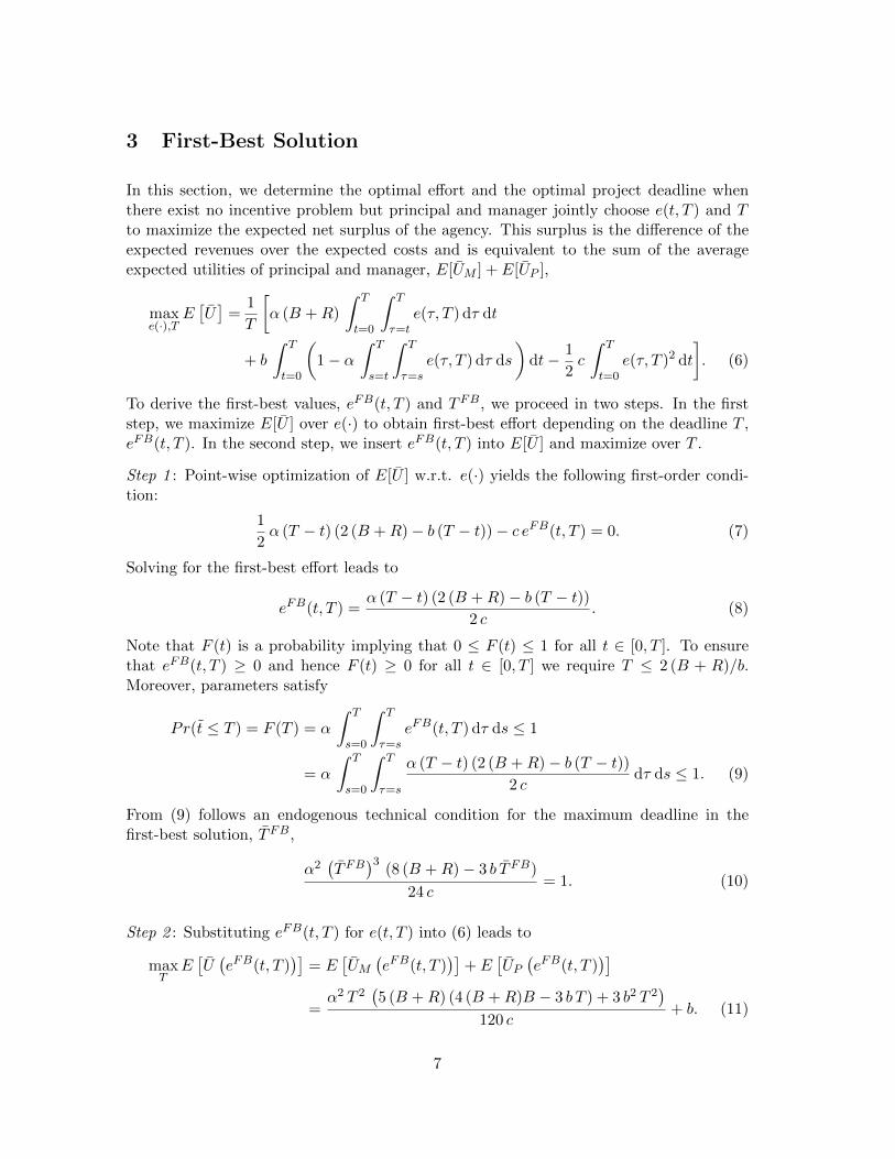
3 First-Best Solution
In this section, we determine the optimal effort and the optimal project deadline whenthere exist no incentive problem but principal and manager jointly choose e(t, T ) and Tto maximize the expected net surplus of the agency. This surplus is the difference of theexpected revenues over the expected costs and is equivalent to the sum of the averageexpected utilities of principal and manager, E[UM ] + E[UP ],
maxe(·),T
E[U]
=1
T
[α (B +R)
∫ T
t=0
∫ T
τ=te(τ, T ) dτ dt
+ b
∫ T
t=0
(1− α
∫ T
s=t
∫ T
τ=se(τ, T ) dτ ds
)dt− 1
2c
∫ T
t=0e(τ, T )2 dt
]. (6)
To derive the first-best values, eFB(t, T ) and TFB, we proceed in two steps. In the firststep, we maximize E[U ] over e(·) to obtain first-best effort depending on the deadline T ,eFB(t, T ). In the second step, we insert eFB(t, T ) into E[U ] and maximize over T .
Step 1 : Point-wise optimization of E[U ] w.r.t. e(·) yields the following first-order condi-tion:
1
2α (T − t) (2 (B +R)− b (T − t))− c eFB(t, T ) = 0. (7)
Solving for the first-best effort leads to
eFB(t, T ) =α (T − t) (2 (B +R)− b (T − t))
2 c. (8)
Note that F (t) is a probability implying that 0 ≤ F (t) ≤ 1 for all t ∈ [0, T ]. To ensurethat eFB(t, T ) ≥ 0 and hence F (t) ≥ 0 for all t ∈ [0, T ] we require T ≤ 2 (B + R)/b.Moreover, parameters satisfy
Pr(t ≤ T ) = F (T ) = α
∫ T
s=0
∫ T
τ=seFB(t, T ) dτ ds ≤ 1
= α
∫ T
s=0
∫ T
τ=s
α (T − t) (2 (B +R)− b (T − t))2 c
dτ ds ≤ 1. (9)
From (9) follows an endogenous technical condition for the maximum deadline in thefirst-best solution, TFB,
α2(TFB
)3(8 (B +R)− 3 b TFB)
24 c= 1. (10)
Step 2 : Substituting eFB(t, T ) for e(t, T ) into (6) leads to
maxT
E[U(eFB(t, T )
)]= E
[UM
(eFB(t, T )
)]+ E
[UP(eFB(t, T )
)]=α2 T 2
(5 (B +R) (4 (B +R)B − 3 b T ) + 3 b2 T 2
)120 c
+ b. (11)
7

Solving the first-order condition, dE[U(eFB(t, T ))
]/dT = 0, such that
d2E[U(eFB(t, T ))
]/dT 2 < 0, yields
0 = 5 (B +R)(8 (B +R)− 9 b TFB
)+ 12 b2
(TFB
)2,
TFB =
(45−
√105)
24· (B +R)
b≈ 1.44804 · (B +R)
b. (12)
We have TFB < 2 (B + R). In addition, (10) requires that TFB ≤ TFB, or, equivalently,that
TFB ≤ 4
(3(
19 +√
105) · c
α2 (B +R)
) 13
≈ 1.87244 ·(
c
α2 (B +R)
) 13
. (13)
We derive the following proposition.
Proposition 1 There is a threshold value, TFB1 = 1.87244 ·(c/(α2 (B +R)
))1/3, such
that a first-best deadline TFB only exists if TFB ≤ TFB1 . Then, in the first-best solution,
eFB(t) =α (TFB − t)
(2 (B +R)− b
(TFB − t
))2 c
, (14)
TFB = 1.44804 · (B +R)
b. (15)
Comparative statics:
1. ∂eFB(t)/∂t
>=<
0 for (B +R)/b
<=>
(TFB − t),2. ∂eFB(t)/∂R = ∂eFB(t)/∂B ≥ 0, and ∂TFB/∂R = ∂TFB/∂B > 0,
3. ∂eFB(t)/∂b ≤ 0, and ∂TFB/∂b < 0,
4. ∂eFB(t)/∂α ≥ 0, and ∂TFB/∂α = 0,
5. ∂eFB(t)/∂c ≤ 0, and ∂TFB/∂c = 0,
6. ∂eFB(t)/∂R = ∂eFB(t)/∂B = ∂eFB(t)/∂b = ∂eFB(t)/∂α = ∂eFB(t)/∂c = 0 if andonly if t = TFB.
Proof: See the Appendix.
From the comparative statics it follows that an effort increasing end-to-end over t cannotbe optimal. Rather, for (B + R)/b ≥ T , the first-best effort eFB is decreasing over t.For (B + R)/b < T , eFB is increasing up to t = TFB − (B + R)/b, and decreasingthereafter. Specifically, (B+R)/b is the total benefit if the project succeeds (B +R) over
8

the manager’s benefit (b) per period of tenure. We call it the success-to-tenure ratio. Bothfirst-best effort and first-best deadline are increasing in the success benefits B and R, butdecrease in the manager’s private tenure benefit b. A higher b ceteris paribus leads to lesseffort: as tenure becomes more valuable the probability for project completion in earlyperiods will be decreased. The endogenous threshold TFB1 limits the project’s successprobability to its feasible value. Consequently, TFB1 increases with the cost factor c, anddecreases with the efficiency parameter α, and the success benefits B + R. That is, thelarger the effort eFB (large α, B, R, small c), the faster is the increase in the project’ssuccess probability, limiting the maximum feasible duration of the project.
4 Project Deadline and Dynamic Moral Hazard
What determines the manager’s optimal choice of effort? Conditional on arrival at datet, an effort e(t, T ) increases the probability of project termination and therewith theprobability of pocketing success benefit B for all t ∈ [t, T ]. However, investing effort iscostly, and the more effort is exerted, the less likely on-the-job benefits b will be retainedin the future. Consequently, at each date t ∈ [0, T ], the manager increases his effort aslong as the benefits associated with this increase outweigh the resulting costs. MaximizingE[UM], as given in (4), point-wise with respect to e(·) yields
0 =1
2α (T − t) (2B − b (T − t))− c e∗(t, T ). (16)
This proves the following proposition.
Proposition 2 The manager’s equilibrium effort is
e∗(t, T ) =α (T − t) (2B − b (T − t))
2 c(17)
for T ≤ 2B/b such that F (t) > 0 holds for all t ∈ [0, T ].
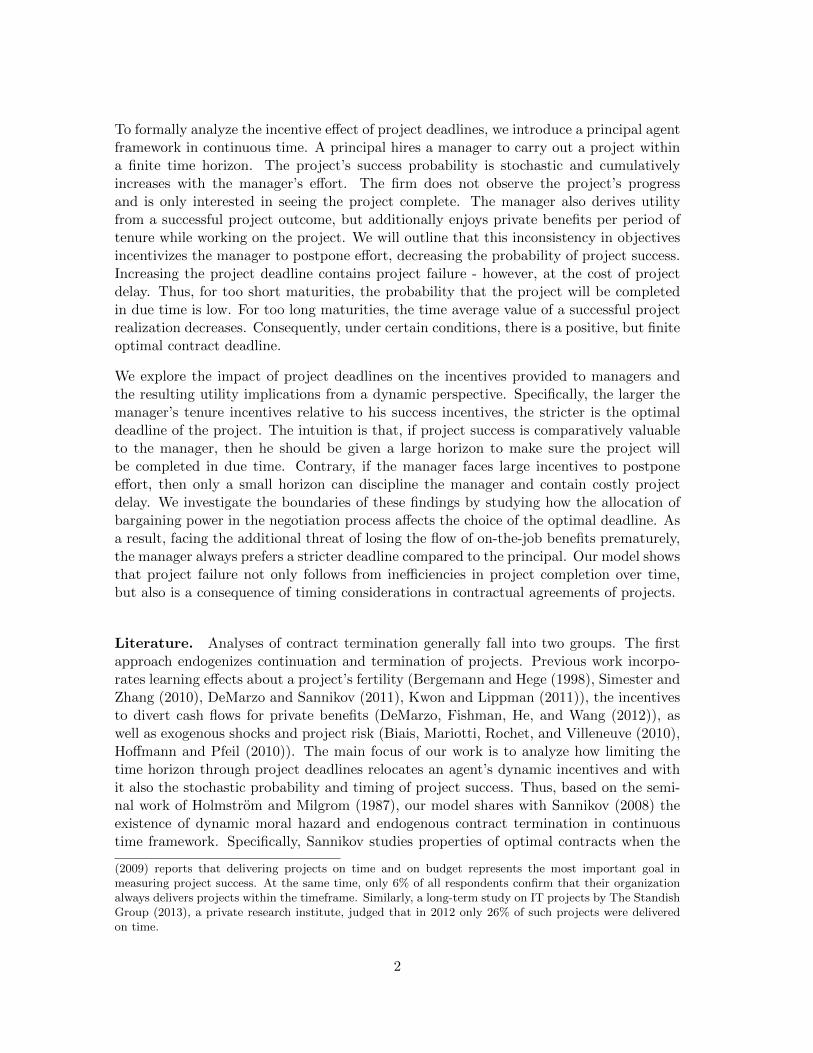
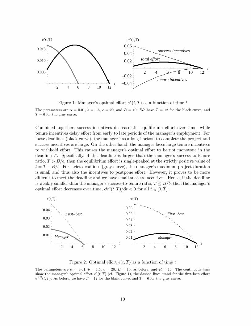
Figure 1 shows the manager’s equilibrium effort e∗(t, T ) as a function of time when varyingthe project deadline T . The right figure decomposes two incentive effects that channelthe manager’s effort over time: success incentives αB (T − t)/c, and tenure incentives−α b (T − t)2/(2 c). First, the larger the success benefit B, the larger are the manager’sincentives to complete the project. As the success probability cumulatively increases withthe manager’s effort, these incentives are most effective for large durations T − t. Second,the optimal effort decreases with the manager’s benefit flow b, as effort diminishes theexpected duration of the project. Moreover, the strength of both effects decreases withthe effort cost factor c, and increases with the efficiency parameter α. Thus, for large T−t,the manager has a long horizon, thus he does not want to “kill the golden goose” at start.Consequently, negative incentives decrease over time, yielding concave tenure incentivesin T − t. For t = T , both effects are zero and the manager exerts no effort at all.
9
2 4 6 8 10 12t
0.005
0.010
0.015
e*Ht,TL
2 4 6 8 10 12t
-0.04
-0.02
0.02
0.04
0.06
e*Ht,TL
success incentives
tenure incentives
total effort
Figure 1: Manager’s optimal effort e∗(t, T ) as a function of time t
The parameters are α = 0.01, b = 1.5, c = 20, and B = 10. We have T = 12 for the black curve, andT = 6 for the gray curve.
Combined together, success incentives decrease the equilibrium effort over time, whiletenure incentives delay effort from early to late periods of the manager’s employment. Forloose deadlines (black curve), the manager has a long horizon to complete the project andsuccess incentives are large. On the other hand, the manager faces large tenure incentivesto withhold effort. This causes the manager’s optimal effort to be not monotone in thedeadline T . Specifically, if the deadline is larger than the manager’s success-to-tenureratio, T > B/b, then the equilibrium effort is single-peaked at the strictly positive value oft = T −B/b. For strict deadlines (gray curve), the manager’s maximum project durationis small and thus also the incentives to postpone effort. However, it proves to be moredifficult to meet the deadline and we have small success incentives. Hence, if the deadlineis weakly smaller than the manager’s success-to-tenure ratio, T ≤ B/b, then the manager’soptimal effort decreases over time, ∂e∗(t, T )/∂t < 0 for all t ∈ [0, T ].
2 4 6 8 10 12t
0.01
0.02
0.03
0.04
eHt,TL
Manager
First-best
2 4 6 8 10 12t
0.01
0.02
0.03
0.04
0.05
0.06
eHt,TL
Manager
First-best
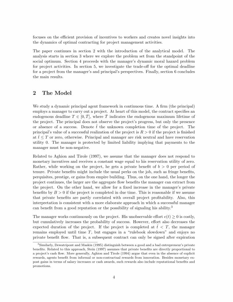
Figure 2: Optimal effort e(t, T ) as a function of time t
The parameters are α = 0.01, b = 1.5, c = 20, B = 10, as before, and R = 10. The continuous linesshow the manager’s optimal effort e∗(t, T ) (cf. Figure 1), the dashed lines stand for the first-best efforteFB(t, T ). As before, we have T = 12 for the black curve, and T = 6 for the gray curve.
10

Figure 2 compares the first-best effort, eFB(t, T ), with the manager’s equilibrium effort,e∗(t, T ), over time. Note that the first-best effort eFB(t, T ) reduces to the manager’soptimal effort e∗(t, T ) when R = 0. Hence, the first-best effort would correspond tothe second-best solution if the manager would internalize the principal’s payoff from theproject. Specifically, the larger the remaining duration of the project T − t, the largeris the difference between the manager’s success incentives, αB (T − t)/c, and the jointsuccess incentives of manager and principal, α (B +R) (T − t)/c. For t = T , both effortscoincide and the optimal effort is zero, eFB(t, T ) = e∗(t, T ) = 0. Hence, the more distantthe deadline, the more the manager underinvests in effort, and the larger is then thedifference in aggregate efforts,
∫ Tt=0(e
FB(t, T )−e∗(t, T )) dt. Therefore, by disregarding theprincipal’s expected value of a success, the manager invests in effort both too little, andtoo late.
5 Optimal Deadline
Let us approach the final question: What is the optimal deadline T ∗ of the project?Initially, this involves the question of how the bargaining power in contract negotiationis allocated between principal and manager. While in many moral hazard agency modelsit is assumed that the principal is endowed with full bargaining, in reality, both partiesenjoy at least some of the bargaining power. In general, given the incentives, any choice ofcontract length is consistent with maximizing the manager’s behavior (manager’s incentivecompatibility constraint). Specifically, incentive compatibility implies that the choice ofthe optimal deadline T ∗ is constrained by the manager’s equilibrium effort e∗(t, T ) asdefined by (17). As F (t) is a probability it follows that 0 ≤ F (t) ≤ 1 for all t ∈ [0, T ].First, T ≤ 2B/b ensures that e∗(t, T ) ≥ 0 and hence F (t) ≥ 0 for all t ∈ [0, T ]. Second,parameters satisfy
Pr(t ≤ T ) = F (T ) = α
∫ T
s=0
∫ T
τ=se∗(t, T ) dτ ds ≤ 1
= α
∫ T
s=0
∫ T
τ=s
α (T − t) (2B − b (T − t))2 c
dτ ds ≤ 1. (18)
From (9) follows an endogenous technical condition for the maximum deadline in thesecond-best solution, TSB,
α2(TSB
)3(8B − 3 b TSB)
24 c= 1. (19)
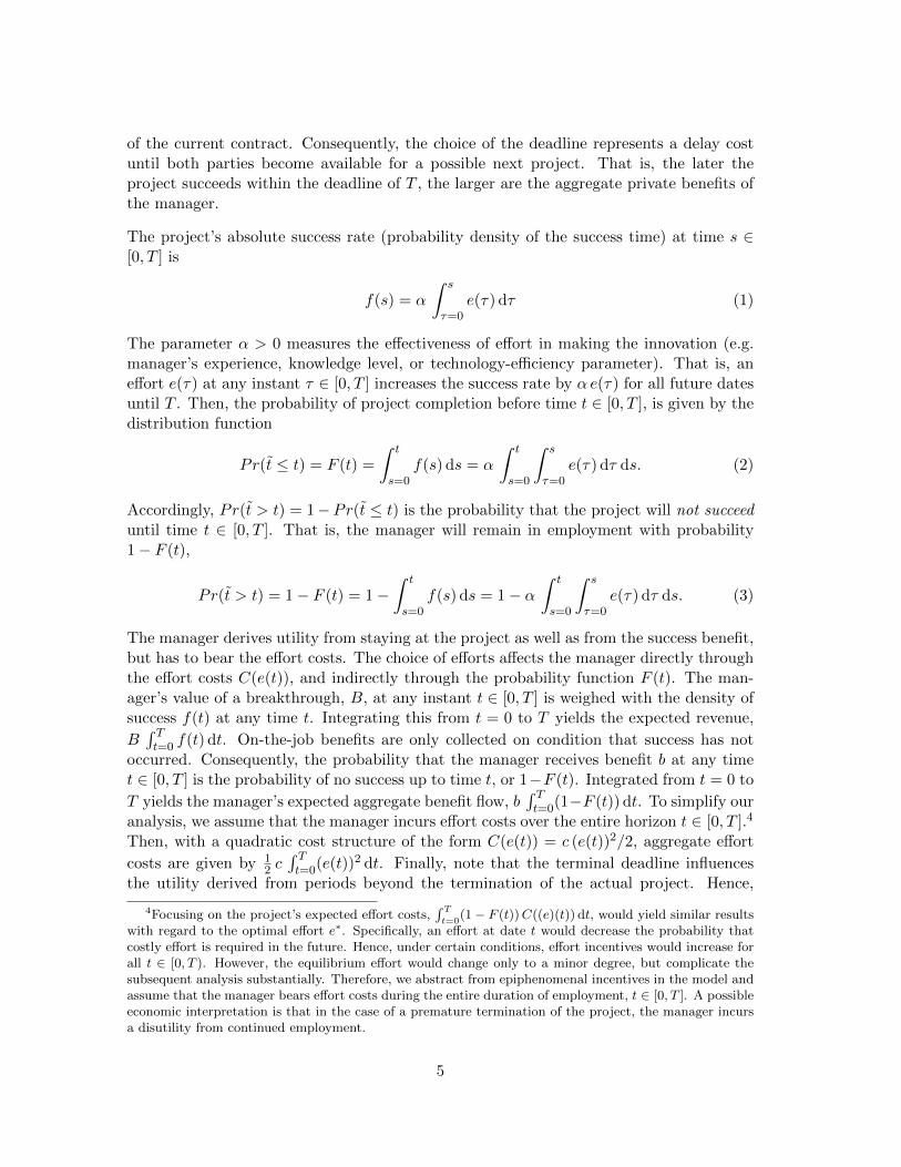
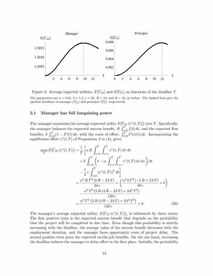
Figure 3 shows manager’s and principal’s average expected utility as dependent on thedeadline T . The dashed lines give the optimal values at the two extremes, when themanager has full bargaining power (in the left picture, T ∗M is approx. 9.5), and when theprincipal enjoys full bargaining power (in the right picture, T ∗P is a little smaller than 12).These boundaries will be analyzed more detailed, before considering the more general caseof arbitrary allocations of bargaining power.
11
2 4 6 8 10 12T
1.5005
1.5010
1.5015
E@U M D
Manager
0 2 4 6 8 10 12T
0.002
0.004
0.006
0.008E@U PD
Principal
Figure 3: Average expected utilities, E[UM ] and E[UP ], as functions of the deadline T
The parameters are α = 0.01, b = 1.5, c = 20, B = 10, and R = 10, as before. The dashed lines give theoptimal deadlines of manager (T ∗M ) and principal (T ∗P ), respectively.
5.1 Manager has full bargaining power
The manager maximizes his average expected utility E[UM (e∗(t, T ))] over T . Specifically,
the manager balances the expected success benefit, B∫ Tt=0 f(t) dt, and the expected flow
benefits, b∫ Tt=0(1 − F (t)) dt, with the costs of effort,
∫ Tt=0C(e(t)) dt. Incorporating the
equilibrium effort e∗(t, T ) of Proposition 2 in (4), gives
maxT
E[UM (e∗(t, T ))] =1
T
[αB
∫ T
t=0
∫ T
τ=te∗(t, T ) dτ dt
+ b
∫ T
t=0
(1− α
∫ T
s=t
∫ T
τ=se∗(t, T ) dτ ds
)dt
− 1
2c
∫ T
t=0(e∗(t, T ))2 dt
]=α2B T 2 (8B − 3 b T )
24 c+
(α2 b T 3 (−5B + 2 b T )
40 c+ b
)− α2 T 2 (5B (4B − 3 b T ) + 3 b2 T 2)
120 c
=α2 T 2
(5B (4B − 3 b T ) + 3 b2 T 2
)120 c
+ b. (20)
The manager’s average expected utility, E[UM (e∗(t, T ))], is influenced by three terms:The first positive term is the expected success benefit that depends on the probabilitythat the project will be completed in due time. Even though this probability is strictlyincreasing with the deadline, the average value of the success benefit decreases with theemployment duration, and the manager faces opportunity costs of project delay. Thesecond positive term gives the expected on-the-job benefits. On the one hand, increasingthe deadline induces the manager to delay effort in the first place. Initially, the probability
12
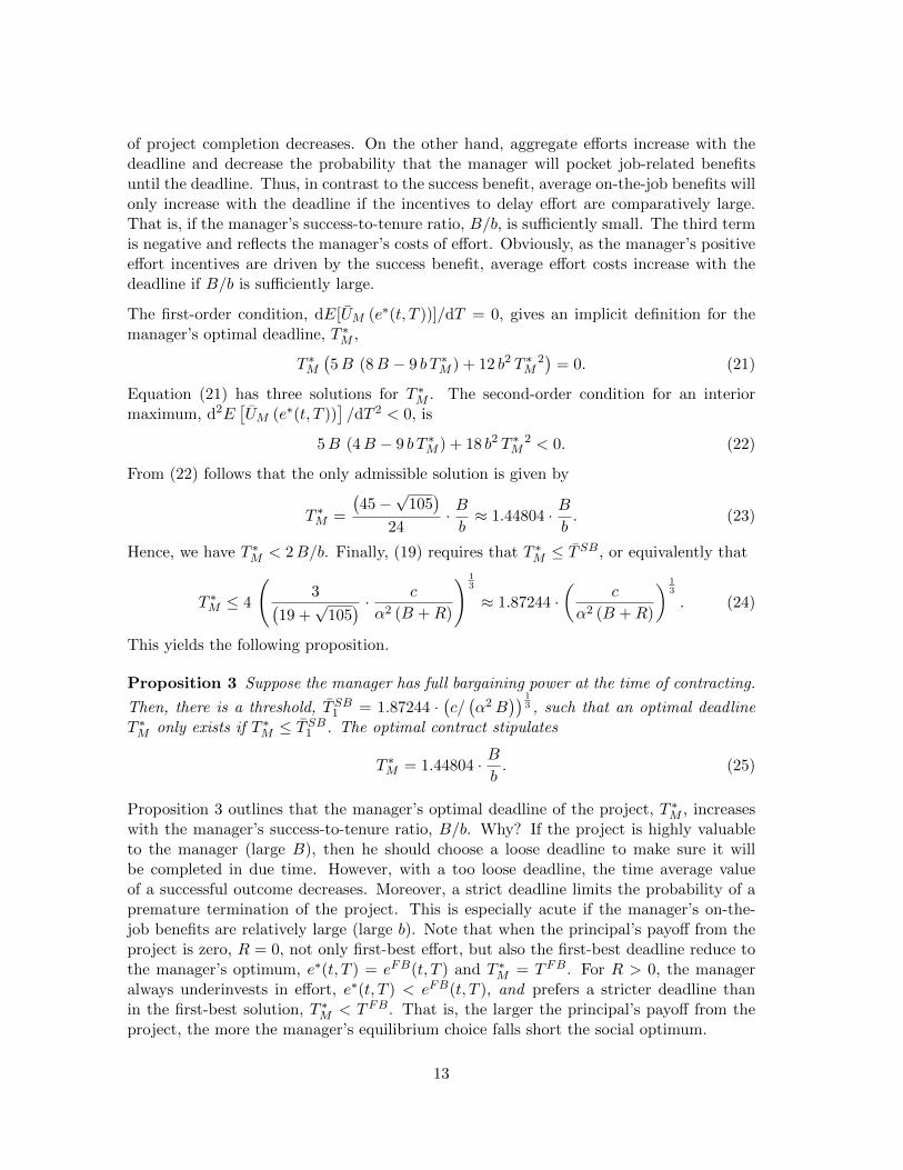
of project completion decreases. On the other hand, aggregate efforts increase with thedeadline and decrease the probability that the manager will pocket job-related benefitsuntil the deadline. Thus, in contrast to the success benefit, average on-the-job benefits willonly increase with the deadline if the incentives to delay effort are comparatively large.That is, if the manager’s success-to-tenure ratio, B/b, is sufficiently small. The third termis negative and reflects the manager’s costs of effort. Obviously, as the manager’s positiveeffort incentives are driven by the success benefit, average effort costs increase with thedeadline if B/b is sufficiently large.
The first-order condition, dE[UM (e∗(t, T ))]/dT = 0, gives an implicit definition for themanager’s optimal deadline, T ∗M ,
T ∗M(5B (8B − 9 b T ∗M ) + 12 b2 T ∗M
2)
= 0. (21)
Equation (21) has three solutions for T ∗M . The second-order condition for an interiormaximum, d2E
[UM (e∗(t, T ))
]/dT 2 < 0, is
5B (4B − 9 b T ∗M ) + 18 b2 T ∗M2 < 0. (22)
From (22) follows that the only admissible solution is given by
T ∗M =
(45−
√105)
24· Bb≈ 1.44804 · B
b. (23)
Hence, we have T ∗M < 2B/b. Finally, (19) requires that T ∗M ≤ TSB, or equivalently that
T ∗M ≤ 4
(3(
19 +√
105) · c
α2 (B +R)
) 13
≈ 1.87244 ·(
c
α2 (B +R)
) 13
. (24)
This yields the following proposition.
Proposition 3 Suppose the manager has full bargaining power at the time of contracting.
Then, there is a threshold, TSB1 = 1.87244 ·(c/(α2B
)) 13 , such that an optimal deadline
T ∗M only exists if T ∗M ≤ TSB1 . The optimal contract stipulates
T ∗M = 1.44804 · Bb. (25)
Proposition 3 outlines that the manager’s optimal deadline of the project, T ∗M , increaseswith the manager’s success-to-tenure ratio, B/b. Why? If the project is highly valuableto the manager (large B), then he should choose a loose deadline to make sure it willbe completed in due time. However, with a too loose deadline, the time average valueof a successful outcome decreases. Moreover, a strict deadline limits the probability of apremature termination of the project. This is especially acute if the manager’s on-the-job benefits are relatively large (large b). Note that when the principal’s payoff from theproject is zero, R = 0, not only first-best effort, but also the first-best deadline reduce tothe manager’s optimum, e∗(t, T ) = eFB(t, T ) and T ∗M = TFB. For R > 0, the manageralways underinvests in effort, e∗(t, T ) < eFB(t, T ), and prefers a stricter deadline thanin the first-best solution, T ∗M < TFB. That is, the larger the principal’s payoff from theproject, the more the manager’s equilibrium choice falls short the social optimum.
13
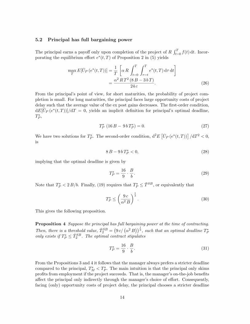
5.2 Principal has full bargaining power
The principal earns a payoff only upon completion of the project of R∫ Tt=0 f(t) dt. Incor-
porating the equilibrium effort e∗(t, T ) of Proposition 2 in (5) yields
maxT
E[UP (e∗(t, T ))] =1
T
[αR
∫ T
t=0
∫ T
τ=te∗(t, T ) dτ dt
]=α2RT 2 (8B − 3 b T )
24 c. (26)
From the principal’s point of view, for short maturities, the probability of project com-pletion is small. For long maturities, the principal faces large opportunity costs of projectdelay such that the average value of the ex post gains decreases. The first-order condition,dE[UP (e∗(t, T ))]/dT = 0, yields an implicit definition for principal’s optimal deadline,T ∗P ,
T ∗P (16B − 9 b T ∗P ) = 0. (27)
We have two solutions for T ∗P . The second-order condition, d2E[UP (e∗(t, T ))
]/dT 2 < 0,
is
8B − 9 b T ∗P < 0, (28)
implying that the optimal deadline is given by
T ∗P =16
9· Bb. (29)
Note that T ∗P < 2B/b. Finally, (19) requires that T ∗P ≤ TSB, or equivalently that
T ∗P ≤(
9 c
α2B
) 13
. (30)
This gives the following proposition.
Proposition 4 Suppose the principal has full bargaining power at the time of contracting.
Then, there is a threshold value, TSB2 =(9 c/
(α2B
)) 13 , such that an optimal deadline T ∗P
only exists if T ∗P ≤ TSB2 . The optimal contract stipulates
T ∗P =16
9· Bb. (31)
From the Propositions 3 and 4 it follows that the manager always prefers a stricter deadlinecompared to the principal, T ∗M < T ∗P . The main intuition is that the principal only skimsprofits from employment if the project succeeds. That is, the manager’s on-the-job benefitsaffect the principal only indirectly through the manager’s choice of effort. Consequently,facing (only) opportunity costs of project delay, the principal chooses a stricter deadline
14

if the manager’s success-to-tenure ratio is comparatively low (small B/b), and vice versa.Note that T ∗P is independent of the principal’s project payoff R: the effect of R is notincluded in the manager’s optimal effort, e∗(t, T ), and hence is not effective in creatingincentives.
From a comparison of the Propositions 1 and 4 it follows that
T ∗P
>=<
TFB for B
>=<
3
√15
7R. (32)
Hence, if the ratio of manager’s to principal’s success benefit B/R is comparatively low(high), then the principal’s optimal deadline is stricter (looser) than in the first-bestsolution, T ∗P < TFB (T ∗P > TFB). The intuition is that the manager does not internalizethe principal’s project payoff which decreases optimal effort and encourages effort delay.This is especially acute if the success benefit the manager can skim from the project iscomparatively low (low B). As the principal cannot rely on monetary incentives to punisheffort delay, he tightens the optimal deadline to make sure that the manager will workeffectively on the project, and vice versa. Note that (32) is independent of the manager’sflow benefit b. The effect of b is completely captured by eFB(t, T ) and TFB, and also bye∗(t, T ) and T ∗P .
5.3 Arbitrary allocations of bargaining power
Now consider the more general case where manager and principal enjoy some of the bar-gaining power at contract negotiation. Specifically, let v ∈ [0, 1] be the manager’s bar-gaining power at the time of contracting. We solve for the asymmetric Nash solution(Binmore, Rubinstein, and Wolinsky, 1986). The main idea is that the equilibrium of abargaining game with alternating offers can be represented by the Nash bargaining so-lution. This definition is equivalent to maximizing the weighted product of the averageexpected individual utilities of manager and principal. Then, using the results of (20) and(26), we obtain
maxT
E[UM (e∗(t, T ))
]vE[UP (e∗(t, T ))
]1−v=
(α2 T 2
(5B (4B − 3 b T ) + 3 b2 T 2
)120 c
+ b
)v
×(α2RT 2 (8B − 3 b T )
24 c
)1−v. (33)
The optimal solution to T can be found through logarithmic transformation,
maxT
v logE[UM (e∗(t, T ))
]+ (1− v) log
[UP (e∗(t, T ))
]= v log
[α2 T 2
(5B (4B − 3 b T ) + 3 b2 T 2
)120 c
+ b
]
+ (1− v) log
[α2RT 2 (8B − 3 b T )
24 c
]. (34)
15

The first-order condition, d(v logE
[UM (e∗(t, T ))
]+ (1− v) log
[UP (e∗(t, T ))
])/dT = 0,
gives an implicit definition for the optimal deadline, T ∗(v),
0 = 120 (1− v) b c (16B − 9 b T ∗(v)) + α2 (T ∗(v))2(
20B2 (16B − 3 (7 + v) b T ∗(v))
+ 3 b2 (T ∗(v))2 ((61 + 16 v)B − 3 (3 + v) b T ∗(v))). (35)
For v = 1 and v = 0, the optimal solutions to the maximization problem are givenby T ∗M ≤ TSB1 and T ∗P ≤ TSB2 , respectively. Hence, for 0 < v < 1, we have T ∗(v) ∈(T ∗M , T
∗P ). Specifically, depending on the manager’s bargaining power, v, we obtain a lower
threshold for the optimal deadline, TSB3 ≤ T ∗(v), that decreases with v. Incorporatingthe endogenous technical condition of (19), which requires that T ∗(v) ≤ TSB, yields
1
140
(105 +
64B
b TSB3
−B(307B − 111 b TSB3
)175B2 − 18 b TSB3
(9B − 4 b TSB3
)) ≤ v. (36)
The second-order condition, d2(v logE
[UM (e∗(t, T ))
]+ (1− v) log
[UP (e∗(t, T ))
])/dT 2 <
0, holds for all T ∗(v) ∈ [T ∗M , T∗P ]. We derive the following proposition.
Proposition 5 Assume that (36) holds. Then, in the Nash bargaining solution, there isan optimal deadline T ∗(v) ≥ TSB3 , with T ∗(v) ∈ [T ∗M , T
∗P ], and T ∗M ≤ TSB1 , T ∗P ≤ TSB2 ,
that is characterized implicitly by
0 = 120 (1− v) b c (16B − 9 b T ∗(v)) + α2 (T ∗(v))2(
20B2 (16B − 3 (7 + v) b T ∗(v))
+ 3 b2 (T ∗(v))2 ((61 + 16 v)B − 3 (3 + v) b T ∗(v))). (37)
Comparative statics:
1. ∂T ∗(v)/∂B > 0,
2. ∂T ∗(v)/∂R = 0,
3. ∂T ∗(v)/∂b < 0,
4. ∂T ∗(v)/∂α ≤ 0,
5. ∂T ∗(v)/∂c ≥ 0,
6. ∂T ∗(v)/∂v < 0,
7. ∂T ∗(v)/∂α = ∂T ∗(v)/∂c = 0 if and only if either v = 0 or v = 1.
Proof: See the Appendix.
Proposition 5 shows that in the asymmetric Nash solution, the optimal deadline T ∗(v)takes values between the individually optimal solutions of manager and principal, T ∗M andT ∗P . Consequently, T ∗(v) increases with the manager’s success-to-tenure ratio, B/b, but is
16

independent of the principal’s payoff R. Accordingly, the optimal deadline decreases withthe manager’s bargaining power v. Note that, for 0 < v < 1, T ∗(v) increases with thecost factor c, and decreases with the efficiency parameter α. The main intuition is that cincreases the marginal costs of effort, decreasing the equilibrium effort and therewith theprobability of project completion. That is, if marginal effort costs increase, then a largerhorizon is required to complete the project. In contrast, α increases the productivity ofeffort in making the innovation, which results in a higher equilibrium effort and a higherprobability of innovation. Therefore, an increase in α decreases the optimal deadline ofthe project.
From an organizational point of view, ex ante bargaining power influences the probabilityby which an innovation is made and, in turn, determines the final value of a project. Withregard to Mr Wowereit, our model accounts for the observation that if tenure benefitsthat may relate to managing a prestigious large-scale project are large (small B/b), thenpremature project completion becomes highly disadvantageous. This causes managers toextract on-the-job benefits to their limits, resulting in project delay and strict deadlineformation. In contrast, if reputational concerns attached to a successful project outcomedominate (large B/b), then effort incentives increase. Like in Mr Wowereit’s second pe-riod of office, it becomes optimal set looser deadlines to make sure the project will befinished timely. However, given any combination of the parameter values, managers al-ways enforce stricter deadlines than it is optimal from the principal’s point of view. Alsofrom the standpoint of the social optimum, they implement too strict deadlines, and alsounderinvest in effort. Thus, if managers can extract on-the-job benefits from working ona project, project completion is threatened by both inefficiencies in effort provision overtime and inefficiencies in contractual agreements on time.
In the context of the empirical literature, our results allow us to reinterpret the so-calledSchumpeterian hypotheses (Schumpeter (1942)) with regard to the labor market. From aSchumpeterian viewpoint, the market power effect states a positive relationship betweena firm’s market power and the supply of innovations. The firm size effect presumes thatlarge firms will be more innovative than small ones (see Kamien and Schwartz (1982) andCohen and Levin (1989), for an overview). In the argumentation of our model, imper-fect competition in the labor market allows firms to determine deadlines as an incentiveinstrument to encourage innovation effort. As a result, greater labor market power atthe firm level increases the optimal deadline of a project and with it the probability ofits completion. Consequently, the presence of ex ante imperfect competition in the labormarket should imply greater flows of innovations. Related to the concept of “creativedestruction”, successful innovations increase a firm’s profits which may increase firm sizeand lead to market concentration in both product and labor markets. Thus, the extentto which labor markets are characterized by imperfect competition ex ante may accountfor ex post market power acquired by successful innovation. Taking a broader view of ourresults, not only innovation effort and project success should considered to be endogenous,but also their effect on market power and firm size. From the viewpoint of public policy,firms’ labor market power may be influenced by labor market regulation, for example withregard to trade unions. Also the implementation of governmental subsidy programs, likein the field of R&D projects, may affect market concentration and firm size. This raises
17

the question about the desirability and the impact of market regulation with regard toboth labor and product markets.
6 Conclusion
In this paper, we investigate the link between deadlines in project management and in-centives for project completion. We show that when managers can skim private benefitsfrom working on a project, they are encouraged to postpone effort. In a trade-off betweensuccess and delay, the optimal project deadline balances the expected increase in projectvalue with the increase in expected project duration and costs. As a result, the largerthe manager’s success incentives relative to his tenure incentives, the smaller is the extentof effort delay and the larger is then the optimal deadline of a project. As another re-sult of the model, the optimal deadline decreases with the manager’s bargaining power atcontract negotiation - imposing additional threat to project success.
Taking a broader view of the results, our work emphasizes the dynamics of project manage-ment activities and contributes to the debate on optimal organizational design of projects.Even though project completion and deadline formation can be influenced by other unmod-eled factors, such as technical requirements, the basic trade-off between effort incentivesand completion time addressed in this paper is in line with the widely observed patternsof projects that mostly fail to succeed within their initial timeframe.
Appendix
Proof of Proposition 1 Substituting eFB (t, T ) into (6) yields
maxT
E[U(eFB(t, T )
)]=E
[UM
(eFB(t, T )
)]+ E
[UP(eFB(t, T )
)]=
1
T
[α (B +R)
∫ T
t=0
∫ T
τ=teFB(t, T ) dτ dt
+ b
∫ T
t=0
(1− α
∫ T
s=t
∫ T
τ=seFB(t, T ) dτ ds
)dt
− 1
2c
∫ T
t=0
(eFB(t, T )
)2dt
]=α2 T 2
(5 (B +R) (4 (B +R)B − 3 b T ) + 3 b2 T 2
)120 c
+ b, (38)
which corresponds to the result of (11). From the first-order-condition,
dE[U(eFB(t, T )
)]dT
=α2 TFB
(5 (B +R)
(8 (B +R)− 9 b TFB
)+ 12 b2
(TFB
)2)
120 c= 0,
(39)
18

we obtain three candidates for an optimum:
TFB1 = 0,
TFB2 =
(45 +
√105)
24· (B +R)
b,
TFB3 =
(45−
√105)
24· (B +R)
b.
Only TFB3 fulfills the second-order-condition,
d2E[U(eFB(t, T )
)]dT 2
=α2(5 (B +R)
(4 (B +R)− 9 b TFB3
)+ 18 b2
(TFB3
)2)
60 c< 0. (40)
Thus,
TFB = TFB3 =
(45−
√105)
24· (B +R)
b≈ 1.44804 · (B +R)
b(41)
if and only if (13) holds.
For the comparative statics with regard to the first-best effort,
eFB (t) =α (TFB − t) (2 (B +R)− b (TFB − t))
2 c,
we have
∂eFB (t)
∂t= −
α(B +R− b
(TFB − t
))c
,
∂eFB (t)
∂B=∂eFB (t)
∂R=α
c
(TFB − t
)≥ 0,
∂eFB (t)
∂b= − α
2 c
(t− TFB
)2 ≤ 0,
∂eFB (t)
∂α=
(TFB − t) (2 (B +R)− b (TFB − t))2 c
≥ 0,
∂eFB (t)
∂c= −α (TFB − t) (2 (B +R)− b (TFB − t))
2 c2≤ 0,
such that for t = TFB,
∂eFB (t)
∂B=∂eFB (t)
∂R=∂eFB (t)
∂α=∂eFB (t)
∂c= 0.
With regard to TFB, we obtain
∂TFB (t)
∂B=∂TFB (t)
∂R=
(45−
√105)
24· 1
b> 0,
∂TFB (t)
∂b= −
(45−
√105)
24· (B +R)
b2< 0.
�
19
Proof of Proposition 5. To prove the comparative static results, we use the implicitfunction theorem. The first-order condition for a maximum requires thatd(v logE
[UM (e∗(t, T ))
]+ (1− v) log
[UP (e∗(t, T ))
])/dT = 0. Differentiating (34) with
respect to T , and equating to zero yields our implicit function, g(T ∗(v), x) = 0. To simplifynotation, we will omit the v in T ∗(v) in the proof. We obtain
g(T ∗, x) =α2 T ∗2 V1 + 120 (1− v) b c (16B − 9 b T ∗)
T ∗ (8B − 3 b T ) (α2 T ∗2 (5B (4B − 3B T ∗) + 3 b2 T ∗2) + 120 b c)= 0, (42)
where
V1 = 20B2 (16B − 3 (7 + v) b T ∗) + 3 b2 T ∗2 ((61 + 16 v)B − 3 (3 + v) b T ∗) , (43)
and x stands for one of the exogenous parameters B, R, b, α, c, and v, respectively. Theexpression in the numerator corresponds to (35) and (37). The comparative static resultsfollow from ∂T ∗/∂x = − (∂g(T ∗, x)/∂x) / (∂g(T ∗, x)/∂T ∗). The second-order conditionfor a maximum requires that the sign of the denominator is negative, ∂g(T ∗, x)/∂T ∗ =d2(v logE
[UM (e∗(t, T ))
]+ (1− v) log
[UP (e∗(t, T ))
])/dT 2 < 0,
∂g(T ∗, x)
∂T ∗=
V2 − 14400 (1− v) b2 c2(32B (4B − 3 b T ∗) + 27 b2 T ∗2
)T ∗2 (8B − 3 b T ∗)2 (α2 T ∗2 (5B (4B − 3 b T ∗) + 3 b2 T ∗2) + 120 b c)2
< 0,
(44)
where
V2 = 240α2 b c T ∗2(9 b3 T 3 ((77− 218 v)B − 9 (1− 3 v) b T ∗)
− 1280B3 ((2− 3 v)B − 3 (1− 2 v) b T ∗)− 12 (197− 488 v) b2B2 T ∗2)
− α4 T ∗4( (
5B (4B − 3 b T ∗) + 3 b2 T ∗2)2 (
32B (4B − 3 b T ∗) + 27 b2 T ∗2)
+ 3 v b2 T ∗2(40B3 (26B − 45 b T ∗) + 16 b2B T ∗2 (69B − 18 b T ∗)
+ 27 b4 T ∗4)). (45)
Equation (45) is strictly negative for T ∗ ∈ [T ∗M , T∗P ]. Now, consider the sign of the nu-
merator, −∂g(T ∗, x)/∂x, for each exogenous parameter. If the first derivative is positive,∂g(T ∗, x)/∂x > 0, then T ∗ is increasing with x, ∂T ∗/∂x > 0. Contrary, if ∂g(T ∗, x)/∂x <
20
0, then we have ∂T ∗/∂x < 0. Taking derivatives, we obtain
∂g(T ∗, B)
∂B=
3 b(V3 + 115200 (1− v) b2 c2
)(8B − 3 b T ∗)2 (α2 T ∗2 (5B (4B − 3 b T ∗) + 3 b2 T ∗2) + 120 b c)2
> 0,
where
V3 = 40α2 c T ∗(80B2 (64 v B + 12 (1− 8 v) b T ∗)− 9 b2 T ∗2
(80 (1− 5 v)B
− (16− 61 v) b T ∗))
+ α4 T ∗4(80 (1 + v)B
(40B3 − 9 b3 T ∗3
)− 20 bB2 T ∗ (16 (15 + 16 v)B − 3 (46 + 49 v) b T ∗) + 9 (8 + 7 v) b4 T ∗4
),
∂g(T ∗, R)
∂R= 0,
∂g(T ∗, b)
∂b= − V4 + 345600 (1− v) b2B c2
(8B − 3 b T ∗)2 (α2 T ∗2 (5B (4B − 3 b T ∗) + 3 b2 T ∗2) + 120 b c)2< 0,
where
V4 = 480α2 c T ∗(80B3 (8 v B + 3 (1− 3 v) b T ∗)− 6 (30− 13 v) b2B2 T ∗2
− 9 b3 T ∗3 (4 (1 + 3 v)B + 3 v b T ∗))
+ 3α4 B T ∗4(80 (1 + v)B
(40B3 − 9 b3 T ∗3
)+ 9 (8 + 7 v) b4 T ∗4
− 20 bB2 T ∗ (16 (15 + 16 v)B − 3 (46 + 49 v) b T ∗)),
∂g(T ∗, α)
∂α=
240 v α b c T ∗(5B (8B − 9 b T ∗) + 12 b2 T ∗2
)(α2 T ∗2 (5B (4B − 3 b T ∗) + 3 b2 T ∗2) + 120 b c)2
≤ 0,
∂g(T ∗, c)
∂c= −
120 v α2 b T ∗(5B (8B − 9 b T ∗) + 12 b2 T ∗2
)(α2 T ∗2 (5B (4B − 3 b T ∗) + 3 b2 T ∗2) + 120 b c)2
≥ 0,
∂g(T ∗, v)
∂v= −
3 b(40 c (16B − 9 b T ∗) + α2 T ∗3 (2B − b T ∗) (10B − 3 b T ∗)
)T ∗ (8B − 3 b T ) (α2 T ∗2 (5B (4B − 3 b T ∗) + 3 b2 T ∗2) + 120 b c)
< 0.
The results hold for all T ∗ ∈ [T ∗M , T∗P ]. At the boundaries, v = 1 and v = 0, we have
T ∗ = T ∗M and T ∗ = T ∗P , respectively, such that
∂g(T ∗, α)
∂α=∂g(T ∗, c)
∂c= 0.
�
References
Aghion, P., and J. Tirole (1994): “The Management of Innovation,” The QuarterlyJournal of Economics, 109(4), 1185–1209.
21
(1997): “Formal and Real Authority in Organizations,” Journal of PoliticalEconomy, 105(1), 1–29.
Bergemann, D., and U. Hege (1998): “Venture Capital Financing, Moral Hazard, andLearning,” Journal of Banking & Finance, 22(6), 703–735.
Biais, B., T. Mariotti, J.-C. Rochet, and S. Villeneuve (2010): “Large Risks,Limited Liability, and Dynamic Moral Hazard,” Econometrica, 78(1), 73–118.
Binmore, K., A. Rubinstein, and A. Wolinsky (1986): “The Nash Bargaining Solu-tion in Economic Modelling,” The RAND Journal of Economics, 17(2), 176–188.
Bonatti, A., and J. Horner (2011): “Collaborating,” The American Economic Review,101(2), 632–663.
(2013): “Career Concerns and Market Structure,” Working Paper, Cowles Foun-dation for Research in Economics, Yale University.
Campbell, A., F. Ederer, and J. Spinnewijn (2014): “Delay and Deadlines: Freerid-ing and Information Revelation in Partnerships,” American Economic Journal: Microe-conomics, 6(2), 163–204.
Cantor, R. (1988): “Work Effort and Contract Length,” Economica, 55(219), 343–353.
Cohen, W. M., and R. C. Levin (1989): “Empirical Studies of Innovation and MarketStructure,” in Handbook of Industrial Organization, ed. by R. Sehmalensee, and R. D.Willig, vol. 2, chap. 18. Elsevier, Amsterdam: North-Holland, 1059-1107.
DeMarzo, P., and Y. Sannikov (2011): “Learning, Termination and Payout Policyin Dynamic Incentive Contracts,” Working Paper, Stanford University and PrincetonUniversity.
DeMarzo, P. M., M. J. Fishman, Z. He, and N. Wang (2012): “Dynamic Agencyand the q Theory of Investment,” The Journal of Finance, 67(6), 2295–2340.
Dewatripont, M., and E. Maskin (1995): “Credit and Efficiency in Centralized andDecentralized Economies,” The Review of Economic Studies, 62(4), 541–555.
Guriev, S., and D. Kvasov (2005): “Contracting on Time,” American Economic Re-view, 95(5), 1369–1385.
Gutierrez, G. J., and P. Kouvelis (1991): “Parkinson’s Law and its Implications forProject Management,” Management Science, 37(8), 990–1001.
Harris, M., and B. Holmstrom (1987): “On the Duration of Agreements,” Interna-tional Economic Review, 28(2), 389–406.
Herweg, F., and D. Muller (2011): “Performance of Procrastinators: On the Valueof Deadlines,” Theory and Decision, 70(3), 329–366.
22
Hoffmann, F., and S. Pfeil (2010): “Reward for Luck in a Dynamic Agency Model,”Review of Financial Studies, 23(9), 3329–3345.
Holmstrom, B., and P. Milgrom (1987): “Aggregation and Linearity in the Provisionof Intertemporal Incentives,” Econometrica, 61, 303–328.
Jovanovic, B. (1979): “Job Matching and the Theory of Turnover,” Journal of PoliticalEconomy, 87(5), 972–990.
Kamien, M. I., and N. L. Schwartz (1982): Market Structure and Innovation. Cam-bridge University Press, Cambridge.
Kwon, H. D., and S. A. Lippman (2011): “Acquisition of Project-Specific Assets withBayesian Updating,” Operations Research, 59(5), 1119–1130.
Lewis, T. R. (2012): “A Theory of Delegated Search for the Best Alternative,” TheRAND Journal of Economics, 43(3), 391–416.
O’Donoghue, T., and M. Rabin (1999): “Incentives for Procrastinators,” The Quar-terly Journal of Economics, 114(3), 769–816.
Parkinson, C. N. (1957): Parkinson’s Law, and Other Studies in Administration. Ran-dom House Inc., New York.
Radner, R. (1981): “Monitoring Cooperative Agreements in a Repeated Principal-AgentRelationship,” Econometrica, pp. 1127–1148.
Saez-Marti, M., and A. Sjogren (2008): “Deadlines and Distractions,” Journal ofEconomic Theory, 143(1), 153–176.
Sannikov, Y. (2008): “A Continuous-Time Version of the Principal-Agent Problem,”The Review of Economic Studies, 75(3), 957–984.
Schumpeter, J. A. (1942): Capitalism, Socialism and Democracy. Harper, New York.
Simester, D., and J. Zhang (2010): “Why Are Bad Products So Hard to Kill?,” Man-agement Science, 56(7), 1161–1179.
Stein, J. C. (1997): “Internal Capital Markets and the Competition for Corporate Re-sources,” The Journal of Finance, 52(1), 111–133.
The Economist (2009): “Closing the Gap: The Link Between Project ManagementExcellence and Long-Term Success,” October 2009.
The Standish Group (2013): “CHAOS Manifesto 2013,” Economic Report.
Townsend, R. M. (1982): “Optimal Multiperiod Contracts and the Gain from EnduringRelationships under Private Information,” The Journal of Political Economy, 90(6),1166.
23

Toxvaerd, F. (2006): “Time of the Essence,” Journal of Economic Theory, 129(1),252–272.
(2007): “A Theory of Optimal Deadlines,” Journal of Economic Dynamics andControl, 31(2), 493–513.
Yang, J. (2010): “Timing of Effort and Reward: Three-Sided Moral Hazard in aContinuous-Time Model,” Management Science, 56(9), 1568–1583.
24