dong liu lei liu‡, ying guo §, xinsheng zhang ¶ arxiv:2110
TRANSCRIPT

Simultaneous Cluster Structure Learning and Estimation of
Heterogeneous Graphs for Matrix-variate fMRI Data
Dong Liu∗, Changwei Zhao†, Yong He,† Lei Liu‡, Ying Guo§, Xinsheng Zhang¶
Abstract: Graphical models play an important role in neuroscience studies, particularly in brain con-
nectivity analysis. Typically, observations/samples are from several heterogenous groups and the group
membership of each observation/sample is unavailable, which poses a great challenge for graph structure
learning. In this article, we propose a method which can achieve Simultaneous Clustering and Estima-
tion of Heterogeneous Graphs (briefly denoted as SCEHG) for matrix-variate function Magnetic Resonance
Imaging (fMRI) data. Unlike the conventional clustering methods which rely on the mean differences of
various groups, the proposed SCEHG method fully exploits the group differences of conditional dependence
relationships among brain regions for learning cluster structure. In essence, by constructing individual-level
between-region network measures, we formulate clustering as penalized regression with grouping and spar-
sity pursuit, which transforms the unsupervised learning into supervised learning. An ADMM algorithm
is proposed to solve the corresponding optimization problem. We also propose a generalized criterion to
specify the number of clusters. Extensive simulation studies illustrate the superiority of the SCEHG method
over some state-of-the-art methods in terms of both clustering and graph recovery accuracy. We also apply
the SCEHG procedure to analyze fMRI data associated with ADHD (abbreviated for Attention Deficit Hy-
peractivity Disorder), which illustrate its empirical usefulness. An R package “SCEHG” to implement the
method is available at https://github.com/heyongstat/SCEHG.
Keyword: Clustering; Graphical model; Matrix data; Network analysis; Penalized method.
∗Shanghai University of Finance and Economics, Shanghai, China;†Zhongtai Institute for Financial Studies, Shandong University, Jinan, China; Corresponding author,
Email:[email protected].‡Division of Biostatistics, Washington University in St.Louis, St. Louis, USA;§Department of Biostatistics and Bioinformatics, Rollins School of Public Health, Emory University, Atlanta, USA;¶Department of Statistics, School of Management, Fudan University, Shanghai, China;
1
arX
iv:2
110.
0451
6v1
[st
at.M
E]
9 O
ct 2
021

1 Introduction
In neuroscience studies, Brain Connectivity Analysis (BCA) has been at the foreground to uncover the
potential pathogenic mechanism of mental disease such as Alzheimer’s disease. Graphical models, which
capture the (conditional) dependence relationships among a set of variables, particularly suit to BCA and
serves as a powerful tool in neuroscience studies. One of the most popular graphical models is the Gaussian
Graphical Model (GGM), and it is well known that recovering the structure of a GGM is equivalent to
finding the support of the corresponding precision matrix. In the high-dimensional case where the number
of covariates can be much larger than the sample size, various penalized methods have been proposed to
estimate the GGM, see for example, Meinshausen and Buhlmann (2006); Yuan and Lin (2007); Cai et al.
(2011); He et al. (2017b).
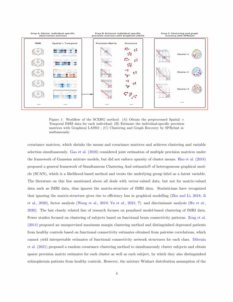
Functional magnetic resonance imaging (fMRI) has been the mainstream imaging modality in neuro-
science research. It records the blood oxygen level dependent time series. fMRI data are in matrix-form
with spatial (brain regions) by temporal (time points) structure, see Figure 1 (A). There also has been many
literature on graphical modeling for matrix-valued data such as fMRI data, see for example, Leng and Tang
(2012); Zhou (2014); Xia and Li (2017). In neuroscience studies, it is often the case that observations are
from several distinct subpopulations/groups. A naive approach is to learn a graphical model for each group
separately/independently. However, such a method inevitably ignores the common structure shared across
different groups and is thus less inefficient and suboptimal. To fully excavate the common structure across
groups, series of joint estimation methods have been proposed during the last decade, see for example, Guo
et al. (2011); Danaher et al. (2014); Cai et al. (2016); He et al. (2017a) for vector-valued data and Zhu and
Li (2018) for matrix-valued data.
All aforementioned literature crucially assume that the group label of each observation is given/known in
priori, which maybe not the case in real application such as online advertising (an important task of which
is to target advertising better for a given user in an online context with group label of each user unknown).
Clustering analysis is an essential tool for unsupervised machine learning to identify groups of objects of the
similar pattern. With dissimilarity structure defined for each pair of objects (users in the context of online
advertising), many well-known clustering algorithms such as K-means, K-medoids, hierarchical clustering can
be applied. One serious limitation of these traditional methods is the non-convexity of the corresponding
optimization problems. In the high-dimensional setting, clustering analysis with feature selection have drawn
increasing attentions, see for example, Pan and Shen (2007); Li et al. (2021).
In many real applications, in addition to grouping objects of the similar pattern, one may also be interested
in understanding conditional dependence relationships among object attributes, which in turn helps to
2

improve grouping/clustering accuracy. The methods for joint estimation of multiple graphs mentioned above
are not directly applicable as all those methods require that the group membership of each object is known
in advance. One may of course first do clustering analysis and then estimate the graphs of each “clustered”
group with memberships of objects obtained from the clustering analysis. However, the estimation accuracy
of graph structures by this naive method heavily relies on the performance of different clustering algorithms
and can not deal with the case that the number of underlying clusters grows with the sample size. Thus
it’s urgent to propose a method which can simultaneously conduct object clustering and joint graphical
model estimation, especially in the era of big data. In this paper, we propose a method which can achieve
Simultaneous Clustering and Estimation of Heterogeneous Graphs (SCEHG) for matrix-valued fMRI data.
The typical characteristic of fMRI data is that it’s in matrix-form and objects from different groups share the
same zero mean matrix but different covariance structures due to the the centralization preprocess step (Chen
et al., 2021). Thus the clustering methods which rely on the mean difference of groups do not work for fMRI
data. Also, the estimation methods of graphical models for vector-valued data do not work (well) for fMRI
data. To overcome the challenge, we first construct individual-level between-region network measures for each
subject by assuming a Kronecker product covariance matrices framework for fMRI data, see Figure 1 (B).
We then formulate the unsupervised clustering task as a supervised penalized regression learning task with
grouping/fusion and sparsity penalty. The fusion penalty is for the purpose of clustering and sparsity penalty
is for recovering sparse graph structures for heterogeneous groups. A MDC-ADMM algorithm is proposed to
solve the corresponding optimization problem and a generalized criterion to specify the number of clusters
is also proposed. Both simulation study and real fMRI data analysis example show the superiority of the
proposed SCEHG method. As a by-product of this new method, we make R package SCEHG implementing
MDC-ADMM algorithm available at GitHub at https://github.com/heyongstat/SCEHG.
1.1 Closely Related Literature Review
In the literature, a closely related line of research focuses on clustering with fusion penalties which apply to all
the pairwise differences of centroids, and these methods are typically known as regression/fusion-based clus-
tering methods, see for example, Pan et al. (2013); Wu et al. (2016); Zhang et al. (2019). Regression/fusion-
based clustering methods show an advantage in some complex clustering situations such as when non-convex
clusters exist, in which traditional clustering methods K-means break down (Pan et al., 2013). The current
work follows this line of research, but considers an additional sparsity penalty in the optimization problem
to achieve variable selection. Another closely related line of research focuses on both graphical model and
clustering at the same time. Zhou et al. (2009) proposed a regularized Gaussian mixture model with general
3
fMRI Spat ial × T emporal Precision Matrix Structure
Cluster 1
Cluster 2
Cluster 3
Step A: Obtain individual-specific observat ion matrices
Step B: Est imate individual-specific precision matrices with Graphical LASSO
Step C: Clustering and graph recovery with SPRclust
… … … … …
AA BB CC
Figure 1: Workflow of the SCEHG method: (A) Obtain the preprocessed Spatial ×Temporal fMRI data for each individual; (B) Estimate the individual-specific precisionmatrices with Graphical LASSO ; (C) Clustering and Graph Recovery by SPRclust si-multaneously.
covariance matrices, which shrinks the means and covariance matrices and achieves clustering and variable
selection simultaneously. Gao et al. (2016) considered joint estimation of multiple precision matrices under
the framework of Gaussian mixture models, but did not enforce sparsity of cluster means. Hao et al. (2018)
proposed a general framework of Simultaneous Clustering And estimatioN of heterogeneous graphical mod-
els (SCAN), which is a likelihood-based method and treats the underlying group label as a latent variable.
The literature on this line mentioned above all deals with vector-valued data, but not for matrix-valued
data such as fMRI data, thus ignores the matrix-structure of fMRI data. Statisticians have recognized
that ignoring the matrix-structure gives rise to efficiency loss in graphical modelling (Zhu and Li, 2018; Ji
et al., 2020), factor analysis (Wang et al., 2019; Yu et al., 2021; ?) and discriminant analysis (Hu et al.,
2020). The last closely related line of research focuses on penalized model-based clustering of fMRI data.
Fewer studies focused on clustering of subjects based on functional brain connectivity patterns. Zeng et al.
(2014) proposed an unsupervised maximum margin clustering method and distinguished depressed patients
from healthy controls based on functional connectivity estimates obtained from pairwise correlations, which
cannot yield interpretable estimates of functional connectivity network structures for each class. Dilernia
et al. (2021) proposed a random covariance clustering method to simultaneously cluster subjects and obtain
sparse precision matrix estimates for each cluster as well as each subject, by which they also distinguished
schizophrenia patients from healthy controls. However, the mixture Wishart distribution assumption of the
4

subject-level precision matrix may deviate from the reality and the assumption of independent observations
within each subject is violated for fMRI data which exhibit autocorrelation .
1.2 Contributions and Structure of the Paper
First we propose a general framework for clustering and variable selection in Section 2. We used the non-
convex penalty in Pan et al. (2013) for grouping pursuit which enforces the equality among some unknown
subsets of parameter estimates. Different from Pan et al. (2013), we add a LASSO penalty to encourage the
sparsity of parameter estimates. We will see that the LASSO penalty is indispensable in terms of recovering
sparse graphs of heterogeneous groups with fMRI data in Section 3. We name the clustering method as
sparse penalized regression-based clustering (SPRclust). For the corresponding optimization problem, we
also combine difference of convex (DC) programming with the alternating direction method of multipliers
(ADMM) as in Pan et al. (2013), but modifies the ADMM algorithm to further deal with the additional L1
penalty part and thus we named the algorithm as MDC-ADMM (with the first M abbreviated for Modified).
We prove the convergence of the MDC-ADMM algorithm and also propose a new criterion to select the tuning
parameters which takes both the clustering performance and variable selection performance into account.
In Section 3 we introduce how we achieve Simultaneous Clustering and Estimation of Heterogeneous
Graphs (SCEHG) of fMRI data with the SPRclust method presented in Section 2, see also Figure 1 (C). We
will see that the proposed procedure allows for the serial correlation of observations within each subject, thus
fits to the analysis of fMRI data better compared with the independent assumption in Dilernia et al. (2021).
Our method also serves as the first (as far as we know) clustering method based on covariance structure
difference rather than mean difference of various groups, which is particularly suitable for fMRI data as the
preprocessed fMRI data are usually demeaned. The SCEHG takes the serial autocorrelation of fMRI data
into account when constructing the individual region-by-region connectivity strength and thus relaxes the
i.i.d. assumptions in Chen et al. (2021); Dilernia et al. (2021).
Extensive simulation studies in Section 4 show the superiority of the proposed SCEHG method over
some state-of-the-art methods. In Section 5 we analyzed a real fMRI dataset associated with ADHD by
the SCEHG method and the findings are consistent with existing literature. We discuss the limitations of
SCEHG method and possible future directions in Section 6.
To end this section, we introduce some notations used throughout the study. Let a+ denotes the positive
part of a. For a vector µ = (µ1, . . . , µp)> ∈ Rp, let ||µ||1 =
∑pi=1 |µi| and ||µ||2 =
√∑pi=1 µ
2i . For a matrix
Xn×p, let X·j be the j-th column of X and Xij be its (i, j)-th element. Denote Ip be the p-dimensional
identity matrix. Furthermore, we denote the trace of X as Tr(X) and the determinant of X as |X|. Let
5

||X||1 be the `1 norm, that is the sum of the absolute values of all the elements of X. We denote by Vec(X)
the vector obtained by stacking the columns of X. Let Vec(X)j>i be the operator that stacks the columns
of the upper triangular elements of matrix X excluding the diagonal elements to a vector. The notation ⊗
represents Kronecker product. For a set F , denote by ]F the cardinality of F .
2 A General Framework for Clustering and Variable Selection
In this section, we introduce a general framework for achieving clustering and parameter estimate sparsity
simultaneously. In Section 2.1, we introduce the model setup with the optimization problem. In Section 2.2,
we introduce the MDC-ADMM algorithm for solving the optimization problem and study its convergence
property. In Section 2.3, we propose a new criterion for tuning parameter selection.
2.1 Model Setup
Given dataset Xn×p = (x>1 ,x>2 , · · · ,x>n )> with observations xi = (xi1, xi2, · · · , xip)>, i = 1, . . . , n, we aim
to conduct cluster analysis to identify group-memberships of the observations such that the within-group
similarity and between-group dissimilarity are strong.
We assume that each data point xi has its own centroid µi = (µi1, µi1, · · · , µip)>, which can be its mean
or median (or other measure), depending on the application. Our goal is to estimate µi while acknowledging
the possibility that many µi’s would be equal if their corresponding xi’s are from the same cluster. We
adopt the fusion penalty to encourage the equality of the centroids. To alleviate the bias of the usual
convex `2-norm group penalty, we adopt the non-convex grouped truncated LASSO penalty as in Pan et al.
(2013), motivated by the Truncated `1 Penalty (TLP) function in Shen et al. (2012). TLP acts as the
surrogate of `0 penalty function and enjoys the advantages stated as “adaptive model selection through
adaptive shrinkage”, “piecewise linearity” and “low resolutions” by Shen et al. (2012). We also add the
`1-norm penalty of centroids to achieve sparsity of the centroids’ estimates, which plays pivotal role in graph
recovery introduced in Section 3.
Summarizing the discussion above, we consider the following optimization problem:
minµ,θ
S(µ,θ) =1
2
n∑i=1
‖xi − µi‖22 + λ1
n∑i=1
‖µi‖1 + λ2∑i<j
TLP(‖θij‖2 ; τ
)subject to θij = µi − µj , 1 ≤ i < j ≤ n.
(2.1)
where TLP(a, b) = min(|a|, b) and λ1, λ2 are two tuning parameters which controls the sparsity and grouping
6

effect, respectively. By solving the above optimization problem, we obtain the estimates of the centroids,
denoted as µi, 1 ≤ i ≤ n. Then the observations with equal estimated centroids are naturally clustered
together and the estimated centroids show sparsity due to the first `1 penalty in (2.1). The clustering method
is named as sparse penalized regression-based clustering (SPRclust). The sparsity of the estimated centroids
is of great importance as it leads to the sparsity of the edges in heterogeneous graphs for fMRI data discussed
in Section 3. In the following we first discuss the computational aspects of the optimization problem.
2.2 Computational Aspects
2.2.1 Algorithm Implementation
The optimization problem in (2.1) is non-convex on θij and can be similarly solved by a modified DC-ADMM
as in Wu et al. (2016). Let S(µ,θ) = S1(µ,θ)− S2(θ) where
S1(µ,θ) =1
2
n∑i=1
‖xi − µi‖22 + λ1
n∑i=1
||µi||1 + λ2∑i<j
||θij ||1, S2(θ) = λ2∑i<j
(||θij ||2 − τ)+.
Note that S1 and S2 are both convex functions and now S(µ,θ) is decomposed into the difference of these
two convex functions. We then construct a sequence of lower approximations of S2(θ), namely S(m)2 (θ),
S(m)2 (θ) = S2(θ(m)) + λ2
∑i<j
(||θij ||2 − ||θ(m)ij ||2)I(||θ(m)
ij ||2 ≥ τ),
where θ(m)ij is the estimate from the m-th iteration. Thus the corresponding S(m+1)(θ,µ) can be given as
S(m+1)(θ,µ) =1
2
n∑i=1
‖xi − µi‖22 + λ1
n∑i=1
||µi||1 + λ2∑i<j
||θij ||2I(||θ(m)ij ||2 < τ)
+ λ2τ∑i<j
I(||θ(m)ij ||2 ≥ τ).
Apparently, S(m+1)(θ,µ) is an upper approximation of S(θ,µ) and it’s convex over θ and µ. So (2.1) can
be rewritten as
minθ,µ
S(m+1)(θ,µ), subject to θij = µi − µj , 1 ≤ i < j ≤ n. (2.2)
7

Optimization Function
𝑆(𝝁, 𝜽)Optimization Function
𝑆(𝝁, 𝜽)
Decomposition
Two Convex Functions
𝑆 𝝁, 𝜽 = 𝑆1 𝝁, 𝜽 − 𝑆2(𝝁, 𝜽)
Upper
Approximation
𝑆(1) 𝝁, 𝜽 = 𝑆1 𝝁,𝜽 − 𝑆2(0)(𝝁, 𝜽) 𝑆(2) 𝝁, 𝜽 = 𝑆1 𝝁, 𝜽 − 𝑆2
(1)(𝝁, 𝜽)
ෝ𝝁(1), 𝜽(1)
Limit Point of The ADMM
ADMM
ෝ𝝁(1), 𝜽(1)
Limit Point of The ADMM
ADMM
……
Limit Point of The MDC-ADMM
ෝ𝝁(𝑚∗), 𝜽(𝑚
∗)
ෝ𝝁𝑖(0)
= 𝒙𝑖, 𝜽𝑖𝑗(0)
= 𝒙𝑖 − 𝒙𝑗 , ෝ𝒗𝑖𝑗(0)
= 𝟎.
Initial Value
……
Figure 2: Illustration of the MDC-ADMM Algorithm.
Following Boyd et al. (2011), we form the scaled augmented Lagrangian function as
Lρ(θ,µ) =1
2
n∑i=1
‖xi − µi‖22 + λ1
n∑i=1
||µi||1 + λ2∑i<j
||θij ||2I(||θ(m)ij ||2 < τ)
+ λ2τ∑i<j
I(||θ(m)ij ||2 ≥ τ) +
ρ
2
∑i<j
||θij − (µi − µj) + vij ||22 −ρ
2
∑i<j
||vij ||22, (2.3)
where vij = yij/ρ, yij is the dual variable. The parameter ρ affects the speed of convergence (Boyd et al.,
2011; Wu et al., 2016) and we set it as 0.4 in our simulation study. Then we perform standard ADMM
procedure as
µk+1i =argmin
µi
1
2||xi − µi||22 + λ1||µi||1 +
ρ
2
∑j>i
||θkij − (µi − µkj ) + vkij ||22 (2.4)
+ρ
2
∑j<i
||θkji − (µk+1j − µi) + vkji||22,
θk+1ij =argmin
θij
λ2τ + ρ2 ||θij − (µk+1
i − µk+1j ) + vkij ||22, if ||θ(m)
ij ||2 ≥ τ ;
λ2||θij ||2 + ρ2 ||θij − (µk+1
i − µk+1j ) + vkij ||22, if ||θ(m)
ij ||2 < τ ;
vk+1ij =vkij + θk+1
ij − (µk+1i − µk+1
j ), 1 ≤ i < j ≤ n,
where superscript k + 1 means the (k + 1)-th step of ADMM iterations.
For the optimization in (2.4) to get the estimate µk+1i , we can construct pseudo observations (z∗i ,y
∗i ) to
8

reformulate the problem as a standard LASSO problem. The first p rows of (z∗i ,y∗i ) correspond to (Ip,xi) and
the rest rows are constructed according to the last two terms of equation (2.4). Specifically, we construct
the pseudo observations (z∗i ,y∗i ) as follows:
(z∗1 ,y∗1) =
√ρ
2
1√ρIp
1√ρx1
Z2(1) Y2(1)
, (z∗n,y∗n) =
√ρ
2
1√ρIp
1√ρxn
Z1(n) Y1(n)
,
and
(z∗i ,y∗i ) =
√ρ
2
1√ρIp
1√ρxi
Z1(i) Y1(i)
Z2(i) Y2(i)
, 1 < i < n,
where
(Z1(i),Y1(i)) =
−Ip θk1i − µk+11 + vk1i
−Ip θk2i − µk+12 + vk2i
......
−Ip θk(i−1)i − µk+1(i−1) + vk(i−1)i
, (Z2(i),Y2(i)) =
Ip θki(i+1) + µk(i+1) + vki(i+1)
Ip θki(i+2) + µk(i+2) + vki(i+2)
......
Ip θkin + µkn + vkin
.
Thus, to update µk+1i is equivalent to solving the following optimization problem:
µk+1i = argmin
µi
‖y∗i − z∗i µi‖22 + λ1‖µi‖1
, (2.5)
from which we can see it’s a standard LASSO problem and we use the cyclic coordinate descent algorithm
to solve it (Friedman et al., 2010).
Similar to the group LASSO optimization problem in Yuan and Lin (2006), we update θkij by soft
thresholding operator, that is
θk+1ij =
µk+1i − µk+1
j − vkij , if ||θ(m)ij ||2 ≥ τ ;
proxλ2/ρ(µk+1i − µk+1
j − vkij), if ||θ(m)ij ||2 < τ ;
where proxs(t) = (1− s/||t||2)+t.
As an illustration, the whole MDC-ADMM algorithm is summarized in Algorithm 1, see also the workflow
in Figure 2.
9

Algorithm 1 MDC-ADMM Algorithm
Require: Dataset X = x1, · · · ,xn ; tuning parameters λ1, λ2, τ and ρ.
1: Initialize: Set m = 0, v(0)ij = 0, µ
(0)i = xi and θ
(0)ij = xi − xj for 1 ≤ i < j ≤ n.
2: while m = 0 or S(µ(m), θ(m)
)− S
(µ(m−1), θ(m−1)
)< 0 do
3: m← m+ 14: Update µ(m) and θ(m) based on (2.4) until the convergence of ADMM.5: end while
Ensure: Estimated centroids µ1, µ2, · · · , µn and a assigned cluster label for each observation.
2.2.2 Algorithm Convergence
In Algorithm 1, for each iteration m of the ADMM algorithm, µ(0)i = xi and θ
(0)ij = xi − xj for 1 ≤ i < j ≤
n are used as the starting values; (µ(m+1), θ(m+1)) is the limit point of the ADMM iterations, or equivalently,
is a minimizer of the Lagrangian function in (2.3). (µ(m+1), θ(m+1)) is then exploited to update the objective
function S(m+1)(µ,θ) as a new approximation to S(µ,θ). We iterate the above process until the stopping
criteria are met. We have the following theorem which guarantee the convergence of the MDC-ADMM
algorithm.
Theorem 2.1. In MDC-ADMM, S(µ,θ) converges in a finite number of steps; that is, there is a m∗ <
∞ with
S(µ(m),θ(m)
)= S
(µ(m∗),θ(m
∗))
for m ≥ m∗.
Moreover,(µ(m∗),θ(m
∗))
is a KKT point.
Remark 2.2. Although ADMM algorithm ensures a global minimizer as S(m)(µ,θ) is closed, proper and
convex, MDC-ADMM only guarantee a KKT point as a result of the nonconvexity of S(µ,θ). A variant
DC algorithm by Breiman and Cutler (1993) can give a global minimizer, but the drawback lies in its
slow convergence speed. We prefer the present version for its faster convergence for large-scale problems.
Furthermore, MDC-ADMM may yield different KKT points with different starting values even for the same
dataset and parameters. However, as shown in our simulation study, the MDC-ADMM algorithm with the
proposed initial values performs well for our purpose.
2.3 Criterion for Selecting Tuning Parameters
For the optimization problem in (2.1), we have three tuning parameters to be determined, i.e., τ, λ1, and λ2.
In TLP penalty, τ controls the tolerance of ||θij ||2. In our paper, we choose the tuning parameters τ, λ1, λ2
by grid search. For criteria of grid search, Pan et al. (2013) and Ghadimi et al. (2014) suggested GCV or the
stability-based criterion based on (adjusted) rand index. However, these criteria are not directly applicable
10

in our case as they ignores measuring the variable selection performance of the additional LASSO penalty.
This poses a great challenge for tuning parameters selection in our setting. To overcome the challenge, we,
as far as we know for the first time, propose a criterion to balance the performances of both clustering and
variable selection for heterogeneous groups simultaneously. Our idea is motivated by the S4 criterion by
Li et al. (2021), abbreviated for “Subsampling Score incorporating Sensitivity and Specificity”. The main
idea of the S4 criterion is that the more stably the method performs, the better the tuning parameters are.
It has achieved success in yielding good performance by measuring the stability of clustering in repeated
subsampled data. In the following, we introduce our criterion for selecting (λ1, λ2, τ) in detail.
For each candidate tuning parameter combination (λ1, λ2, τ), we first obtain the estimated centroids of
observations Xn×p by solving (2.1) and the corresponding clustering result. We then use a matrix Tn×n =
(Tij) to record the clustering result where Tij indicates whether sample i and sample j are in the same
cluster: Tij = 1 if samples i and j belong to the same cluster and 0 otherwise. Then we generate B sets
of subsampled data, denoted as X(1)[r·n]×p,X
(2)[r·n]×p, · · · ,X
(B)[r·n]×p, where r ∈ (0, 1) is the resampling fraction.
Similarly, we can obtain T(b)n×n = (T
(b)ij ) for b = 1, 2, · · · , B. Missing value label “NA” is assigned to T
(b)ij if
one or both of the two samples i and j are not in the b-th subsampling dataset. We take element-wise
average of T (b) to derive the mean comembership matrix T sub = T subij , where T subij indicates the frequency
that sample i and sample j are clustered together across all B subsampling procedure. Missing values are
omitted when taking average. The concordance score of sample i is defined as
Ci =
∑j 6=i T
subij I(Tij = 1)∑
j 6=i I(Tij = 1)+
∑j 6=i(1− T subij )I(Tij = 0)∑
j 6=i I(Tij = 0)− 1, i = 1, 2, · · · , n
where I(·) is the indicator function. Assuming that the comembership matrix T is the underlying truth, the
first term can be viewed as sensitivity score of sample i and the second term as specificity score of sample i.
In our definition of Ci, it is close to 1 when sample i is a stably clustered subject but approaches 0 if
sample i is an outlier. We then truncate the lower α% of Ci to avoid the impact of potential outliers and
define C as the trimmed mean of Ci.
The concordance score of features can be defined similarly as follows. As the nonzero locations of
the centroids may differ a lot across clusters, we consider the concordance score of features cluster by
cluster. We first resort to the estimates of the centroids, µi = (µi1, . . . , µip)> to calculate fk = (fkj),
where j = 1, . . . , p, k = 1, 2, · · · , K, where K is the corresponding estimated number of clusters. We set
fkj = I((∑i∈Ck I(µij 6= 0)/|Ck|) > 0.5
), where Ck is the label set of samples collected in the k-th cluster.
Similarly, f(b)k can be obtained by B times resampling and fsubkj = (
∑Bb=1 f
(b)kj )/B is the proportion that
feature j is selected among B times subsampling procedure. Then the concordance score of features in the
11

k-th cluster can be defined as
F (k) =
∑pj=1 f
subkj I(fkj = 1)∑p
j=1 I(fkj = 1)+
∑pj=1(1− fsubkj )I(fkj = 0)∑p
j=1 I(fkj = 0)− 1,
If the estimated number of clusters for X(b)[r·n]×p is larger than that for Xn×p, we omit this resampling dataset
since F is not well defined. For simplicity, we take the average of F (k) over k, denote as F , to represent
the concordance score of features corresponding to the given (λ1, λ2, τ). Then our criterion to select tuning
parameters can be summarized as follows:
1. Calculate C and F for each possible combination of (λ1, λ2, τ).
2. Choose the combinations whose C are among the top s% and denote the set as A .
3. Choose the optimal combination (λ1, λ2, τ)opt which corresponds to the maximum F in A , i.e.,
(λ1, λ2, τ)opt = argmax(λ1,λ2,τ)∈A F .
Remark 2.3. We always omit the cases when all features are selected together or K = 1, as in these cases
the denominator of the second term of Ci or F (k) (specificity) is zero and the corresponding score is not well-
defined. Our criterion first guarantees the performance of clustering and then guarantees the performance
of variable selection. There are other ways to select the best tuning parameters based on C and F such
as (λ1, λ2, τ)opt = arg maxλ1,λ2,τ (ω1C + ω2F ) or (λ1, λ2, τ)opt = arg maxλ1,λ2,τ
√(ω1C × ω2F ) where 0 <
ωi < 1 and ω1 + ω2 = 1. The performances of these criteria are comparable by our simulation study.
Throughout this paper, we set r = 0.5, s% = 0.4, α% = 0.2 and B = 5 in both simulation study and real
data analysis.
3 Simultaneous Clustering and Estimation of Heterogeneous Graphs
with fMRI Data
In this section, we introduce the SCEHG method that simultaneously conducts clustering and estimation of
heterogeneous graphical models for matrix-variate fMRI data. We first review the definition of matrix-normal
distribution for characterizing the distribution of matrix-variate fMRI data. The framework is scientifically
plausible in neuroimaging studies, see for example Xia and Li (2017); Zhu and Li (2018); Chen et al. (2021)
Definition 3.1. A matrix-variate Zp×q follows the matrix-normal distribution, denoted as
Zp×q ∼MN (Mp×q,ΣT ⊗ΣS),
12

if and only if Vec(Zp×q) follows a multivariate normal distribution i.e.
Vec(Zp×q) ∼ N (Vec(Mp×q),ΣT ⊗ΣS),
where ΣS = (ΣS,ij) ∈ Rp×p and ΣT = (ΣT,ij) ∈ Rq×q denotes the covariance matrices of p spatial locations
and q times points, respectively.
By the matrix-normal framework, we have Cov−1(Vec(Zp×q)) = Σ−1T ⊗Σ−1S = ΩT⊗ΩS , where ΩS denote
the spatial precision matrix and ΩT the temporal precision matrix. The primary interest is to recover the
connectivity network characterized by the spatial precision matrix ΩS while the temporal precision matrix
ΩT is treat as a nuisance parameter.
3.1 Individual-specific between-region connectivity measures
In the section, we introduce the procedure to construct the individual-specific between-region connectivity
measures by estimating the spatial precision matrix for each subject. The technique is growing popular
recently, also known as constructing “functional connectivity network predictors” for each subject, see for
example, Chen et al. (2021); Weaver et al. (2021). Both work omit the serial dependence of fMRI data and
simply take the individual sample covariance matrix as the input of CLIME (Cai et al., 2011) or Graphical
LASSO (Yuan and Lin, 2007) algorithm. In this article, in view of the serial dependence of fMRI data, we
propose a nonparametric method to estimate the spatial covariance matrix of each individual.
Assume that there exist K clusters and let Ck be the label set of samples collected in the k-th cluster
and n =∑Kk=1 |Ck|. The preprocessed fMRI data are demeaned and thus the first moment information is
not helpful for clustering, and clustering methods based on mean difference are invalid such as K-means. We
assume that
Zγk ∼MN (0,ΣTk ⊗ΣSk), γk ∈ Ck, k ∈ 1, 2, . . . ,K,
and without loss of generality, assume the diagonal elements of ΣTk are ones. At each time point t ∈
1, 2, · · · , q, we have Zγk·t ∼ N (0,ΣSk). If the class label set Ck is known in advance, there exists many
algorithms to estimate Σ−1S in the high-dimensional setting such as CLIME or Graphical LASSO. In the
current work we tackle an unsupervised learning problem, i.e., Ck is unknown. We aim to cluster the samples
and recover the heterogeneous networks between brain regions of K groups simultaneously. We take the serial
dependence of fMRI data into account to estimate the spatial covariance matrix for each sample Zγ ∈ Rp×q
(note that there is no subscript k in γ henceforth). In detail, we use the kernel method to estimate the
13

individual-specific spatial covariance matrix at time point t as:
ΣγS(t) =
∑s ωstZ
γ·s(Z
γ·s)>∑
s ωst, (3.1)
from which we can see that ΣγS(t) is a weighted covariance matrix of Zγ·s, with weights ωsj = K(|s− j|/hn)
given by a symmetric nonnegative kernel over time. We set hn = n1/3 and use Gaussian kernel in (3.1).
Finally, we set ΣγS =
∑qt=1 Σγ
S(t)/q and use the graphical LASSO to estimate the individual-specific precision
matrix ΩγS ,
ΩγS = argmin
ΩTr
(ΣγSΩ)− log |Ω|+ λ||Ω||1, γ ∈ 1, 2 . . . , n. (3.2)
where the tuning parameter λ is chosen by cross validation.
3.2 SCEHG Method
In this section, we formally introduce our SCEHG method. First, we straighten the upper triangular matrix
of ΩγS without diagonal elements and treat them as new features. Then we adopt the SPRclust method
proposed in section 2 to achieve clustering and estimation of heterogeneous graphs simultaneously. In
detail, let xγ = Vec(ΩγS)j>i, γ = 1, 2, · · · , n and xγ is a p(p − 1)/2 dimensional vector. Then we denote
Aγ ∈ Rp×p, γ = 1, 2, · · · , n and solve the following optimization problem:
minAγ ,θ
S(µ,θ) =1
2
n∑γ=1
‖xγ −Vec(Aγ)j>i‖22 + λ1
n∑γ=1
||Vec(Aγ)j>i||1 + λ2∑s<t
TLP (‖θst‖2 ; τ)
subject to θst = Vec(As)j>i −Vec(At)j>i, 1 ≤ s < t ≤ n.
(3.3)
Optimization problem (3.3) is in essence the same with optimization problem (2.1) and can be solved by
the MDC-ADMM algorithm. The SCEHG method takes advantage of the the SPRclust in the following
two aspects: (I) the features of SPRclust in the fMRI setting are the individual-specific between-region
connectivity measures, i.e., the functional connectivity network predictors (Chen et al., 2021; Weaver et al.,
2021), and we cluster the samples by their second moment covariance information rather than the mean; (II)
as SPRclust achieve sparsity of the estimated centroids, in the current setting, it means that the solutions of
optimization problem (3.3), i.e., Aγ , γ = 1, . . . , n are sparse, from which we can recover the edges of graphs
by the nonzero locations of Aγ .
14

4 Simulation Studies
In this section, we conduct simulation studies to assess the performance of the proposed SCEHG method
in terms of both clustering and graph recovery. We consider the following method for comparison: PRclust
method by Wu et al. (2016), SCAN method by Hao et al. (2018) and sparse K-Means (SKM) by Witten and
Tibshirani (2010). For the SKM method, we select the tuning parameters involved by the S4 criterion in Li
et al. (2021). For the SCAN method, an initial value for the number of clusters should be given in advanced
and we simply set it as the true number of clusters.
For simplicity, we consider generating data from a matrix-normal distribution with different ΣSk but the
same ΣT in all clusters, that is
Zγk ∼MN (0,ΣT ⊗ΣSk), γk ∈ Ck, k ∈ 1, 2, . . . ,K.
We set the true number of clusters as K = 3 and |Ck| ∈ 10, 15, p ∈ 10, 15 and q = 100. The covariance
matrices structures are introduced in detail below.
We consider two types of ΣT which are common in fMRI data: the first type is the auto-regressive
(AR) correlation, where (ΣT )st = 0.5|s−t|; and the second type is band correlation (BC), where (ΣT )st =
1/(|s− t|+1) for |s− t| < 4 and 0 otherwise. As for ΣSk , we first introduce how we construct its inverse ΩSk ,
which characterizes the graph structures of K groups. We also consider two types of graph structure GS :
the Hub structure and the Small-World structure. We resort to R package “huge” to generate Hub structure
with 3 non-overlapping graph and use R package “rags2ridges” to generate 3 Small-World graph. For further
details of these two graph structures, one may refer to Zhao et al. (2012) and Chen et al. (2021). We design
the precision matrices of K = 3 groups such that all share the same graph structure (either Hub or Small-
World) but with different partition blocks, illustrated by the heat map of the precision matrices in Figure 3.
The covariance matrices ΣSk are set to be Ω−1Sk .
To conclude, we consider four scenarios according to the structures of ΣSk and ΣT :
• Scenario 1: ΣT is of AR covariance structure and ΣSk is based on GS with Hub structure.
• Scenario 2: ΣT is of AR covariance structure and ΣSk is based on GS with Small-World structure.
• Scenario 3: ΣT is of BD covariance structure and ΣSk is based on GS with Hub structure.
• Scenario 4: ΣT is of BD covariance structure and ΣSk is based on GS with Small-World structure.
In the following we introduce related indexes to evaluate the performance of our SCEHG method in
terms of both clustering and graph recovery. The Rand index, adjusted Rand index (aRand) and Jaccard
15

Table 1: Simulation Results for Scenario 1. Freq a|b, a and b are the frequency ofoverestimating and underestimating the cluster numbers, respectively. The values in theparentheses denote standard deviation.
(nk, p,K) MethodClustering-related Indexes Graph Recovery Indexes
Kmean Freq Rand aRand Jaccard TPR TNR FDR
(10, 10, 3)
SCEHG 2.8600 0|14 0.9678 0.9375 0.9404 0.9026(0.1362) 0.8304(0.1321) 0.5600(0.1544)SKM 2.9500 4|10 0.9686 0.9356 0.9347 0.7750(0.3208) 0.4271(0.4824) 0.6486(0.3928)
PRclust 2.7600 0|22 0.9402 0.8908 0.9011 0.9993(0.0115) 0.0284(0.0458) 0.8933(0.0134)SCAN 1.0000 0|53 0.3103 0.0000 0.3103 1.0000(0.0000) 0.0061(0.0137) 0.8957(0.0013)
(10, 15, 3)
SCEHG 2.9800 2|4 0.9881 0.9766 0.9772 0.8582(0.1506) 0.8207(0.0886) 0.6922(0.0835)SKM 2.9800 2|4 0.9882 0.9759 0.9757 0.6717(0.3829) 0.4546(0.4927) 0.6522(0.4346)
PRclust 2.9400 0|6 0.9862 0.9732 0.9745 0.9929(0.0323) 0.0743(0.0801) 0.9182(0.0068)SCAN 1.0000 0|3 0.3103 0.0000 0.3103 1.0000(0.0000) 0.0447(0.0060) 0.9205(0.0005)
(15, 10, 3)
SCEHG 2.8600 0|14 0.9682 0.9384 0.9417 0.9061(0.1371) 0.8339(0.1032) 0.5713(0.1344)SKM 2.9100 4|13 0.9664 0.9333 0.9346 0.6760(0.3454) 0.6022(0.4723) 0.5473(0.4324)
PRclust 2.8600 0|14 0.9682 0.9384 0.9417 0.9993(0.0115) 0.0092(0.0195) 0.8954(0.0113)SCAN 1.0000 0|52 0.3182 0.0000 0.3182 0.9971(0.0208) 0.0011(0.0049) 0.8965(0.0018)
(15, 15, 3)
SCEHG 2.9600 1|5 0.9885 0.9777 0.9787 0.8742(0.1426) 0.8158(0.0943) 0.6925(0.0817)SKM 2.9800 2|4 0.9894 0.9789 0.9788 0.5725(0.3815) 0.6025(0.4820) 0.5636(0.4664)
PRclust 2.9300 0|7 0.9841 0.9692 0.9708 0.9992(0.0102) 0.0324(0.0447) 0.9214(0.0036)SCAN 1.0000 0|42 0.3182 0.0000 0.3182 0.9960(0.0180) 0.0129(0.0132) 0.9232(0.0017)
Table 2: Simulation results for Scenario 2, Freq a|b, a and b are the frequency of over-estimating and underestimating the cluster numbers, respectively. The values in theparentheses denote standard deviation.
(nk, p,K) MethodClustering-related Indexes Graph Recovery Indexes
Kmean Freq Rand aRand Jaccard TPR TNR FDR
(10, 10, 3)
SCEHG 2.9800 0|2 0.9954 0.9911 0.9915 0.8509(0.1463) 0.9156(0.0891) 0.2663(0.1787)SKM 3.1200 12|0 0.9934 0.9838 0.9787 0.7765(0.3389) 0.3536(0.4626) 0.6413(0.3464)
PRclust 2.9900 2|3 0.9927 0.9856 0.9859 0.9825(0.0537) 0.0786(0.0965) 0.8106(0.0427)SCAN 1.0000 0|54 0.3103 0.0000 0.3103 1.0000(0.0000) 0.0095(0.0168) 0.8208(0.0025)
(10, 15, 3)
SCEHG 3.0100 1|0 0.9998 0.9995 0.9993 0.7138(0.1801) 0.8979(0.0799) 0.3335(0.1338)SKM 3.0700 7|0 0.9973 0.9935 0.9914 0.6973(0.4178) 0.3447(0.4695) 0.6428(0.3551)
PRclust 6.1900 54|0 0.9552 0.8826 0.8556 0.8982(0.1311) 0.2497(0.2091) 0.7699(0.0549)SCAN 1.0000 0|5 0.3103 0.0000 0.3103 1.0000(0.0000) 0.0306(0.0158) 0.8047(0.0026)
(15, 10, 3)
SCEHG 2.9400 0|6 0.9864 0.9736 0.9750 0.8298(0.1510) 0.9315(0.0747) 0.2305(0.1807)SKM 3.1000 10|0 0.9948 0.9876 0.9838 0.6504(0.3702) 0.5631(0.4714) 0.5338(0.3990)
PRclust 2.9600 0|4 0.9909 0.9824 0.9833 0.9900(0.0398) 0.0444(0.0675) 0.8160(0.0370)SCAN 1.0000 0|49 0.3182 0.0000 0.3182 0.9981(0.0132) 0.0107(0.0181) 0.8209(0.0033)
(15, 15, 3)
SCEHG 3.0100 1|0 0.9999 0.9997 0.9996 0.7239(0.1871) 0.8923(0.0854) 0.3401(0.1368)SKM 3.0400 4|0 0.9981 0.9953 0.9939 0.6680(0.4250) 0.3833(0.4795) 0.6238(0.3663)
PRclust 6.1100 61|0 0.9666 0.9175 0.8951 0.9326(0.1188) 0.1656(0.1904) 0.7845(0.0462)SCAN 1.0000 0|18 0.3182 0.0000 0.3182 0.9981(0.0079) 0.0146(0.0113) 0.8075(0.0019)
16

Table 3: Simulation results for Scenario 3, Freq a|b, a and b are the frequency of over-estimating and underestimating the cluster numbers, respectively. The values in theparentheses denote standard deviation.
(nk, p,K) MethodClustering-related Indexes Graph Recovery Indexes
Kmean Freq Rand aRand Jaccard TPR TNR FDR
(10, 10, 3)
SCEHG 2.9100 0|9 0.9793 0.9598 0.9617 0.9516(0.1003) 0.7056(0.1306) 0.7025(0.0942)SKM 3.0200 6|4 0.9809 0.9588 0.9555 0.8035(0.3132) 0.3596(0.4697) 0.6880(0.3770)
PRclust 2.7800 0|21 0.9471 0.9008 0.9080 0.9993(0.0115) 0.0198(0.0324) 0.8943(0.0123)SCAN 1.0000 0|58 0.3103 0.0000 0.3103 0.9948(0.0276) 0.0041(0.0109) 0.8964(0.0022)
(10, 15, 3)
SCEHG 2.9700 1|4 0.9883 0.9771 0.9779 0.7309(0.1699) 0.9289(0.0536) 0.4956(0.1481)SKM 3.0000 4|4 0.9877 0.9747 0.9734 0.7058(0.3768) 0.4052(0.4863) 0.6817(0.4189)
PRclust 2.9500 0|5 0.9885 0.9777 0.9787 0.9938(0.0291) 0.0564(0.0623) 0.9198(0.0049)SCAN 1.0000 0|2 0.3103 0.0000 0.3103 1.0000(0.0000) 0.0206(0.0146) 0.9223(0.0011)
(15, 10, 3)
SCEHG 2.9100 0|9 0.9795 0.9604 0.9625 0.9155(0.1280) 0.8133(0.1043) 0.6001(0.1281)SKM 2.9400 3|9 0.9781 0.9568 0.9579 0.7030(0.3348) 0.5819(0.4759) 0.5585(0.4194)
PRclust 2.5500 0|43 0.8932 0.7996 0.8155 1.0000(0.0000) 0.0045(0.0128) 0.8958(0.0109)SCAN 1.0000 0|62 0.3182 0.0000 0.3182 0.9978(0.0169) 0.0021(0.0068) 0.8963(0.0018)
(15, 15, 3)
SCEHG 2.8900 0|11 0.9750 0.9516 0.9542 0.8939(0.1308) 0.7612(0.1139) 0.7391(0.0772)SKM 2.9800 2|4 0.9892 0.9784 0.9782 0.5842(0.3810) 0.5924(0.4839) 0.5695(0.4612)
PRclust 2.9400 0|6 0.9864 0.9736 0.9750 0.9996(0.0072) 0.0209(0.0301) 0.9223(0.0023)SCAN 1.0000 0|12 0.3182 0.0000 0.3182 1.0000(0.0000) 0.0163(0.0082) 0.9226(0.0006)
Table 4: Simulation results for Scenario 4, Freq a|b, a and b are the frequency of over-estimating and underestimating the cluster numbers, respectively. The values in theparentheses denote standard deviation.
(nk, p,K) MethodClustering-related Indexes Graph Recovery Indexes
Kmean Freq Rand aRand Jaccard TPR TNR FDR
(10, 10, 3)
SCEHG 2.9700 0|3 0.9931 0.9866 0.9872 0.8519(0.1421) 0.9189(0.0640) 0.2760(0.1612)SKM 3.1500 14|0 0.9923 0.9810 0.9752 0.8054(0.3191) 0.3238(0.4523) 0.6560(0.3293)
PRclust 3.0300 6|3 0.9919 0.9837 0.9832 0.9860(0.0454) 0.0634(0.0864) 0.8128(0.0411)SCAN 1.0000 0|63 0.3103 0.0000 0.3103 0.9988(0.0093) 0.0109(0.0165) 0.8208(0.0030)
(10, 15, 3)
SCEHG 2.9800 0|2 0.9954 0.9911 0.9915 0.7583(0.1741) 0.8261(0.1032) 0.4561(0.1190)SKM 3.0900 9|0 0.9961 0.9905 0.9874 0.7683(0.3827) 0.2749(0.4399) 0.6761(0.3211)
PRclust 3.0000 0|0 1.0000 1.0000 1.0000 0.9257(0.1244) 0.1520(0.1399) 0.7945(0.0153)SCAN 1.0000 0|4 0.3103 0.0000 0.3103 1.0000(0.0000) 0.0235(0.0166) 0.8058(0.0027)
(15, 10, 3)
SCEHG 2.9300 0|7 0.9841 0.9692 0.9708 0.8105(0.1512) 0.9491(0.0449) 0.2039(0.1505)SKM 3.0800 8|0 0.9957 0.9896 0.9864 0.7133(0.3574) 0.4852(0.4773) 0.5729(0.3775)
PRclust 2.8700 0|13 0.9705 0.9428 0.9458 0.9904(0.0373) 0.0309(0.0549) 0.8185(0.0349)SCAN 1.0000 0|64 0.3182 0.0000 0.3182 1.0000(0.0000) 0.0055(0.0146) 0.8214(0.0022)
(15, 15, 3)
SCEHG 2.9400 0|6 0.9864 0.9736 0.9750 0.7397(0.1795) 0.8673(0.0965) 0.3877(0.1313)SKM 3.0300 3|0 0.9988 0.9972 0.9963 0.6940(0.4137) 0.3625(0.4734) 0.6333(0.3579)
PRclust 2.9600 0|4 0.9909 0.9824 0.9833 0.9593(0.0940) 0.0895(0.1139) 0.8005(0.0133)SCAN 1.0000 0|21 0.3182 0.0000 0.3182 1.0000(0.0000) 0.0190(0.0146) 0.8065(0.0023)
17

Small-World Structure
Figure 3: Heat map of the generated precision matrices of K = 3 clusters. The top panelillustrates the hub structure and the bottom panel illustrates the small-world structure.
index are common indexes for evaluating the performance of clustering methods, see for example, Rand
(1971), Hubert and Arabie (1985) and Wu et al. (2016). The closer the values of these indexes are to 1,
the better the clustering performances are. We also report the mean of the estimated cluster numbers by
various methods over 100 replications, denoted as Kmean and summarize the frequency of overestimating
and underestimating the cluster numbers. To evaluate the performance of graph recovery, we adopt the
common indexes, the true positive rate (TPR), true negative rate (TNR) and false discovery rate (FDR) see
for example, Chen et al. (2021).
The detailed results are shown in Tables 1-4, from which we can see that the proposed SCEHG performs
satisfactorily in various scenarios. We can also see that the SCEHG show advantage over the other three
methods. The SKM method and the PRclust method tend to perform not too badly (at most comparable
with the SCEHG method) in terms of clustering but are much inferior to the proposed SCEHG in terms of
graph recovery. As PRclust cannot achieve sparsity of the estimated centroids, it always leads to high TPR
18

but low TNR. The SCAN method seems to lose power in the designed setting and performs not satisfactorily
in terms of both clustering and graph recovery. To conclude, our SCEHG method shows advantages over
the existing state-of-the-art methods in terms of both clustering and graph structure recovery.
5 Real Analysis of fMRI data related with ADHD
Attention Deficit Hyperactivity Disorder (ADHD), is one of the most common neurodevelopmental disorders
in children. It is estimated that ADHD has a worldwide prevalence of 7.2% among children, the condition
persists into adulthood among 70% of those diagnosed in childhood (Zhao et al., 2017). In this section, we
apply the proposed SCEHG method to analyze a resting state fMRI dataset associated with ADHD. The
dataset is from the ADHD-200 Global Competition, which includes demographical information and resting-
state fMRI of nearly one thousand children and adolescents, including both combined types of ADHD
and typically developing controls (TDC). The data were collected from eight participating sites and we
focus our analysis on the fMRI data from the Beijing site only to avoid potential site bias. The dataset
consists of 183 participants with 74 patients (ADHD) and 109 controls (TDC) and can be downloaded from
https://neurobureau.projects.nitrc.org. To reduce computational burden, we only focus on 52 ADHD
patients and 25 controls from the male participants and partition the standard 116 nodes into 8 brain regions:
Insula, Limbic, Occipital, Parietal, Frontal, Cerebellum, SCGM and Temporal. We then take the average
over each brain region at given time points for each subject, finally leading to spatial dimension p = 8 ,
temporal dimension q = 232 and sample size n = 77 . For each subject, we use the algorithm proposed in
Section 3.1 by the R package “glasso” to obtain the individual precision matrix. Then we use the proposed
SCEHG method to cluster the subjects and estimate the brain connectivity graphs.
Table 5: The clustering results for ADHD and TDC samples.
Group ADHD TDC Total1 49(94.23%) 2(8%) 512 3(5.77%) 23(92%) 26
Total 52 25
The clustering results of the samples are shown in Table 5, from which we can see that most of ADHD
samples are clustered into Group 1, and over 90 percent of TDC samples are clustered into Group 2. The
Rand index and the adjusted Rand index are 0.877 and 0.751, respectively. It has to be pointed out that
the above results are based on a priori that the clustering number is two. Actually, the subjects in Group 1
are indeed clustered into one group by the SCEHG method , while the subjects in Group 2 are not exactly
clustered into one group by SCEHG method. Given the priori that K = 2, the subjects that are not clustered
19

into Group 1 are assigned to Group 2 artificially. In fact, the TDCs may have other potential mental diseases
and there is no guarantee that TDCs can be clustered into the same group by any clustering technique such
as K-means.
Table 6: Proportion of the edges absent in Group 1 while existent in Group 2.
Edge Group 1 Group 2Insula ↔ Limbic 100% 46.2%
Insula ↔ Occipital 94.1% 42.3%Insula ↔ Parietal 94.1% 30.8%Frontal ↔ SCGM 92.2% 42.3%
Insula ↔ Temporal 92.2% 42.3%Limbic ↔ Temporal 90.2% 42.3%
Occipital ↔ Cerebellum 88.2% 34.6%Frontal ↔ Occipital 88.2% 42.3%Limbic ↔ Occipital 84.3% 30.8%Limbic ↔ Parietal 82.4% 42.3%
Frontal ↔ Cerebellum 82.4% 38.5%SCGM ↔ Temporal 82.4% 42.3%Frontal ↔ Limbic 80.4% 26.9%Insula ↔ SCGM 74.5% 38.5%
Next we analyze the resultant brain connectivity graphs and identify the the connectivity networks
between brain regions. By the SCEHG Method proposed in Section 3.2, we obtain the estimates of Aγ
for each subject, denoted as Aγ , γ = 1, 2, · · · , n. Then the proportion of an absence of edge between brain
region i and j in Group k (k = 1, 2) can be calculated by the following formula:
Prop(e(k)ij ) =
∑γ∈Ck I(Aγ,ij = 0)
] Ck
where Ck, k = 1, 2 is the index set of Group k, Aγ,ij is the (i, j)-th entry of Aγ . The connection between
brain region i and j in Group k is thought to be absent if Prop(e(k)ij ) >= 0.5, otherwise there exist an edge
between brain region i and j. The proportions of the edges absent in Group 1 while existent in Group 2 are
displayed in Table 6, while all other edges are absent in two groups. From Table 6, it can be deduced that
the cause of ADHD may be attributed to the absent connections between certain brain regions.
Furthermore, we find that the brain region “Insula” is a hub node in the differential network, which is
shown in Figure 4. We suspect that the brain region “Insula” is impaired in the ADHD patients as the
functional connectivity between this region with other regions are almost all absent in ADHD patients. In
fact it has been proved that the “Insula” brain region is closely related to the pathophysiology of ADHD:
Deficits of the anterior insula (AI) which is involved in salient stimuli allocation might be associated with
the pathophysiology of ADHD according to Zhao et al. (2017), see also Vetter et al. (2018); Belden et al.
20

axial view coronal view sagittal view
Figure 4: The differential network between Group 1 and Group 2 from the axial view,coronal view and sagittal view respectively (left ro right). The red point is “Insula” brainregion.
(2014).
6 Summary and Discussions
Graphical model or network model plays an important role in characterizing the relationship between vari-
ables and has been widely applied in areas such as biology and finance. Most existing literature focuses on
the case that the membership of each observation is known in priori, which may not hold in real application.
For example, in neuroscience studies, one usually does not known how many subtypes of a mental disease
exist. In this article, we propose a method which can achieve clustering and graph recovery simultaneously
for matrix-variate data, motivated by the fMRI technique. In essence, we transform the unsupervised learn-
ing problem into a supervised penalized regression-based problem, with both `1 penalty and fusion penalty.
We propose a MDC-ADMM algorithm for the optimization problem. Both simulation study and real data
analysis show the advantage of the proposed method in terms of both clustering and graph recovery. Lim-
itations of the proposed method lie in its high computation burden when dealing with large-scale problem
(large sample size and dimensionality) and its inability of controlling the resultant number of clusters, which
are common limitations for the fusion-penalty based regression technique for clustering. In future study we
will consider more efficient algorithms or methods to achieve clustering and graph recovery simultaneously
for large-scale problem.
21

Acknowledgements
This work was supported by grants from the National Natural Science Foundation of China (Grant No.
12171282, 11801316, 11971116); Natural Science Foundation of Shandong Province (Grant No. ZR2019QA002);
the Fundamental Research Funds of Shandong University, China; Young Scholars Program of Shandong Uni-
versity, China. We would like to thank professor Will Wei Sun at Purdue University for providing the codes
of their SCAN method.
A Appendix
Proof of Theorem 2.1 The convergence of MDC-ADMM in finite steps attributes to the following three
facts. First, as Lρ(θ,µ) in (2.3) is closed, proper and convex and the unaugmented Lagrangian S(m+1)(θ,µ)
in (2.2) has a saddle point, thus the ADMM algorithm converges to the optimal value, see Boyd et al. (2011).
Second, by construction of S(m)(µ,θ) and S(µ,θ), for each positive integer m, we have
S(µ(m), θ(m)
)= S(m+1)
(µ(m), θ(m)
)≤ S(m)
(µ(m), θ(m)
)≤ S(m)
(µ(m−1), θ(m−1)
)= S
(µ(m−1), θ(m−1)
),
which implies S(µ(m),θ(m)) is non-increasing with respect to m and the equality is established if and only if(µ(m), θ(m)
)=(µ(m−1), θ(m−1)
)as a result of the convergence of ADMM algorithm. Thus the monotonicity
of S(µ(m),θ(m)) with respect to m can be regarded as the stopping criterion. Third, as S(m+1)(µ,θ) depends
on m only through the indicator function I(||θ(m)
ij ||2 ≥ τ)
, which implies S(m+1)(µ,θ) has a finite set of
possible functional forms across all m and this leads to a finite set of distinct minimal values. These facts
imply MDC-ADMM terminates in a finite number of iterations.
Next we show that(µ(m∗),θ(m
∗))
is a KKT point of S(µ,θ). Following Theorem 3.1 of Ye (2004) and Wu
et al. (2016), we can use subgradient to deal with S(µ(m∗),θ(m
∗))
and S(m∗+1)(µ(m∗),θ(m
∗))
as both of
them are Lipschitz functions.
Since the subgradient of the S(µ(m∗),θ(m
∗))
is the same as S(m∗+1)(µ(m∗),θ(m
∗))
and then we simply
verify the KKT condition without inequality constraints, that is
2(z∗)>(y∗ − z∗µ) + sgn(µ) = 0,
λ2bijθij||θij ||2
+ ρ(θij − µi + µj + vij) = 0,
θij = µi − µj ,
22

where sgn(µ) = (sgn(µ1), sgn(µ2), · · · , sgn(µp))>, sgn(x) is the sign function, z = (z>1 , z
>2 , · · · , z>n )> and
bij = I(||θ(m)ij ||2 < τ). Note that
(µ(m), θ(m)
)is the limiting point of the ADMM iterations, thus the first
equation holds under the cyclic coordinate descent algorithm since the target function in (2.5) is convex.
Similarly, the second equation holds under the soft thresholding operator. The last equation holds due to
the fact that the steps of updating vij is the same as the KKT conditions. Thus(µ(m∗),θ(m
∗))
is a KKT
point of S(µ,θ).
References
Belden, A.C., Barch, D.M., Oakberg, T.J., April, L.M., Luby, J.L., 2014. Anterior insula volume and guilt:
Neurobehavioral markers of recurrence after early childhood major depressive disorder. Jama Psychiatry
72.
Boyd, S., Parikh, N., Chu, E., 2011. Distributed optimization and statistical learning via the alternating
direction method of multipliers. Now Publishers Inc.
Breiman, L., Cutler, A., 1993. A deterministic algorithm for global optimization. Mathematical Programming
58, 179–199.
Cai, T., Li, H., Liu, W., Xie, J., 2016. Joint estimation of multiple high-dimensional precision matrices.
Statist. Sinica. 26, 445–464.
Cai, T., Liu, W., Luo, X., 2011. A constrained `1 minimization approach to sparse precision matrix estima-
tion. Journal of the American Statistical Association 106, 594–607. doi:10.1198/jasa.2011.tm10155.
Chen, H., Guo, Y., He, Y., Ji, J., Liu, L., Shi, Y., Wang, Y., Yu, L., Zhang, X., 2021. Simultaneous differ-
ential network analysis and classification for matrix-variate data with application to brain connectivity.
Biostatistics, in press .
Danaher, P., Wang, P., Witten, D.M., 2014. The joint graphical lasso for inverse covariance estimation across
multiple classes. J. R. Stat. Soc. Ser. B. Stat. Methodol. 76, 373–397.
Dilernia, A., Quevedo, K., Camchong, J., Lim, K., Zhang, L., 2021. Penalized model-based clustering of
fMRI data. Biostatistics, in press .
Friedman, J., Hastie, T., Tibshirani, R., 2010. Regularization paths for generalized linear models via coor-
dinate descent. Journal of statistical software 33, 1.
23

Gao, C., Zhu, Y., Shen, X., Pan, W., 2016. Estimation of multiple networks in gaussian mixture models.
Electronic Journal of Statistics 10, 1133–1154.
Ghadimi, E., Teixeira, A., Shames, I., Johansson, M., 2014. Optimal parameter selection for the alternating
direction method of multipliers (admm): quadratic problems. IEEE Transactions on Automatic Control
60, 644–658.
Guo, J., Levina, E., Michailidis, G., Zhu, J., 2011. Joint estimation of multiple graphical models. Biometrika
98, 1–15.
Hao, B., Sun, W., Liu, Y., Cheng, G., 2018. Simultaneous clustering and estimation of heterogeneous
graphical models. Journal of Machine Learning Research 18, 1–58.
He, Y., Zhang, X., Ji, J., Liu, B., 2017a. Joint estimation of multiple high-dimensional gaussian copula
graphical models. Australian & New Zealand Journal of Statistics 59, 289–310.
He, Y., Zhang, X., Wang, P., et al., 2017b. High dimensional gaussian copula graphical model with FDR
control. Computational Statistics & Data Analysis 113, 457–474. doi:10.1016/j.csda.2016.06.012.
Hu, W., Shen, W., Zhou, H., Kong, D., 2020. Matrix linear discriminant analysis. Technometrics 62, 196–205.
Hubert, L., Arabie, P., 1985. Comparing partitions. Journal of classification 2, 193–218.
Ji, J., He, Y., Liu, L., Xie, L., 2020. Brain connectivity alteration detection via matrix-variate differential
network model. Biometrics, in press .
Leng, C., Tang, C.Y., 2012. Sparse matrix graphical models. Journal of the American Statistical Association
107, 1187–1200. doi:10.1080/01621459.2012.706133.
Li, Y., Zeng, X., Lin, C.W., Tseng, G., 2021. Simultaneous estimation of number of clusters and feature
sparsity in clustering high-dimensional data. Biometrics, to appear .
Meinshausen, N., Buhlmann, P., 2006. High-dimensional graphs and variable selection with the lasso. The
Annals of Statistics 34, 1436–1462. doi:10.1214/009053606000000281.
Pan, W., Shen, X., 2007. Penalized model-based clustering with application to variable selection. Journal
of Machine Learning Research 8, 1145–1164.
Pan, W., Shen, X., Liu, B., 2013. Cluster analysis: Unsupervised learning via supervised learning with a
non-convex penalty. Journal of Machine Learning Research 14, 1865–1889.
24
Rand, W.M., 1971. Objective criteria for the evaluation of clustering methods. Journal of the American
Statistical association 66, 846–850.
Shen, X., Pan, W., Zhu, Y., 2012. Likelihood-based selection and sharp parameter estimation. Journal of
the American Statistical Association 107, 223–232.
Vetter, N.C., Buse, J., Backhausen, L.L., Rubia, K., Smolka, M.N., Roessner, V., 2018. Anterior insula
hyperactivation in adhd when faced with distracting negative stimuli. Human Brain Mapping 39.
Wang, D., Liu, X., Chen, R., 2019. Factor models for matrix-valued high-dimensional time series. Journal
of Econometrics 208, 231–248.
Weaver, C., Xiao, L., Lindquist, M., 2021. Single-index models with functional connectivity network predic-
tors. Biostatistics, in press .
Witten, D.M., Tibshirani, R., 2010. A framework for feature selection in clustering. Journal of the American
Statistical Association 105, 713–726.
Wu, C., Kwon, S., Shen, X., Pan, W., 2016. A new algorithm and theory for penalized regression-based
clustering. Journal of Machine Learning Research 17, 1–25.
Xia, Y., Li, L., 2017. Hypothesis testing of matrix graph model with application to brain connectivity
analysis. Biometrics 73, 780–791. doi:10.1111/biom.12633.
Ye, J.J., 2004. Nondifferentiable multiplier rules for optimization and bilevel optimization problems. SIAM
Journal on Optimization 15, 252–274.
Yu, L., He, Y., Kong, X., Zhang, X., 2021. Projected estimation for large-dimensional matrix factor models.
Journal of Econometrics, in press. doi:10.1016/j.jeconom.2021.04.001.
Yuan, M., Lin, Y., 2006. Model selection and estimation in regression with grouped variables. Journal of
the Royal Statistical Society: Series B (Statistical Methodology) 68, 49–67. doi:10.1111/j.1467-9868.
2005.00532.x.
Yuan, M., Lin, Y., 2007. Model selection and estimation in the gaussian graphical model. Biometrika 94,
19–35. doi:10.1093/biomet/asm018.
Zeng, L., Shen, H., Liu, L., Hu, D., 2014. Unsupervised classification of major depression using functional
connectivity MRI. Human Brain Mapping 35, 1630–1641.
25

Zhang, Y., Wang, H.J., Zhu, Z., 2019. Robust subgroup identification. Statistica Sinica 29, 1873–1889.
Zhao, Q., Hui, L., Yu, X., Fang, H., Wang, Y., Liu, L., Cao, Q., Qian, Q., Zang, Y., Sun, L., 2017.
Abnormal resting-state functional connectivity of insular subregions and disrupted correlation with
working memory in adults with attention deficit/hyperactivity disorder. Frontiers in Psychiatry 8, 200.
Zhao, T., Liu, H., Roeder, K., Lafferty, J., Wasserman, L., 2012. The huge package for high-dimensional
undirected graph estimation in r. Journal of Machine Learning Research 13, 1059–1062.
Zhou, H., Pan, W., Shen, X., 2009. Penalized model-based clustering with unconstrained covariance matrices.
Electronic Journal of Statistics 3, 1473–1496.
Zhou, S., 2014. Gemini: Graph estimation with matrix variate normal instances. Annals of Statistics 42,
532–562. doi:10.1214/13-AOS1187.
Zhu, Y., Li, L., 2018. Multiple matrix gaussian graphs estimation. Journal of the Royal Statistical Society:
Series B (Statistical Methodology) 80, 927–950. doi:10.1111/rssb.12278.
26