don’t forget your roots: constant-time root nding …don’t forget your roots: constant-time root...

Don’t forget your roots: constant-time rootfinding over F2m

Douglas Martins1, Gustavo Banegas2,3, and Ricardo Custodio1

1 Departamento de Informatica e Estatıstica,Universidade Federal de Santa Catarina

Florianopolis, SC, 88040-900, [email protected], [email protected]

2 Department of Mathematics and Computer ScienceTechnische Universiteit Eindhoven

P.O. Box 513, 5600 MB Eindhoven, The Netherlands3 Chalmers University of Technology

Gothenburg, [email protected]

Abstract. In the last few years, post-quantum cryptography has re-ceived much attention. NIST is running a competition to select somepost-quantum schemes as standard. As a consequence, implementationsof post-quantum schemes have become important and with them side-channel attacks. In this paper, we show a timing attack on a code-basedscheme which was submitted to the NIST competition. This timing at-tack recovers secret information because of a timing variance in findingroots in a polynomial. We present four algorithms to find roots that areprotected against remote timing exploitation.

Keywords: Side-channel Attack · Post-quantum Cryptography · Code-based Cryptography · Roots Finding.

1 Introduction

In recent years, the area of post-quantum cryptography has received considerableattention, mainly because of the call by the National Institute of Standards andTechnology (NIST) for the standardization of post-quantum schemes. On thiscall, NIST did not restrict to specific hard problems. However, most schemesfor the Key Encapsulation Mechanism (KEM) are lattice-based and code-based.The latter type is based on coding theory and includes one of the oldest unbrokencryptosystems, namely the McEliece cryptosystem [15].

This study was financed in part by the Coordenacao de Aperfeicoamento de Pessoal de Nıvel Su-perior - Brasil (CAPES) - Finance Code 001; through the European Union’s Horizon 2020 researchand innovation programme under the Marie Sk lodowska-Curie grant agreement No. 643161; andby Sweden through the WASP expedition project Massive, Secure, and Low-Latency Connectivityfor IoT Applications.

2 Douglas Martins, Gustavo Banegas, and Ricardo Custodio

One of the requirements for those proposals is that they are resistant toall known cryptanalysis methods. However, even if a scheme is immune to suchattacks, it may be subject to attacks related to its implementation. In particular,submissions need to avoid side-channel attacks.

There are different ways to apply side-channel attacks to a cryptosystem.As an example, an attacker can measure the execution time of the operationsperformed by an algorithm and, based on these measures, estimate some secretinformation of the scheme. This approach is thriving even in a data communica-tion network environment. Daniel J. Bernstein, for instance, demonstrated howto recover AES keys by doing timing attacks on the cache “access speed” [5].

In code-based cryptography, timing attacks on the decryption process aremostly done during the retrieval of the Error Locator Polynomial (ELP) asshown by [20]. The attack is usually done during the polynomial evaluationprocess, while computing its roots. This attack was demonstrated first in [20]and later in an improved version in [10].

[21] demonstrates algorithms to find roots efficiently in code-based cryp-tosystems. However, the author shows only timings in different types of imple-mentations and selects the one that has the least timing variability. In otherwords, the author does not present an algorithm to find the roots in constanttime and eliminate a remote timing attack as remarked in Section 6 of [22]. Inour work, we use strategies to make the execution time of those algorithms con-stant. The first and most important one is to write the algorithms iteratively,eliminating all recursions. We also use permutations and simulated operationsto uncouple possible measurements of the side effects of the data being mea-sured. The implementation for finding roots in [12] uses Fast Fourier Transform(FFT), which is efficient, but is built and optimized for F213 . In this paper, weaim at developing a more generic implementation that does not require specificoptimization in the finite field arithmetic.

Contributions of this paper: In this paper, we show how to perform a timingattack on a code-based key encapsulation mechanism called BIGQUAKE, whichwas submitted to NIST [2]. The attack was based on timing leakage on rootfinding process on the decoding step. The original implementation submitted toNIST uses a variation of the Berlekamp Trace Algorithm (BTA) to find roots inthe ELP. We provide other methods to find roots and implement them avoidingtiming attacks. Moreover, we make a comparison between methods, showing thenumber of CPU cycles required for our implementation.

Structure of this paper: In Section 2, we give a brief description of Goppa codes,the McEliece cryptosystem and BIGQUAKE for an understanding about howthe cryptosystems work and the basic notation used in this paper. In Subsec-tion 2.4, we show how to use a timing attack for recovering the error vectorin BIGQUAKE. In Section 3, the core of the paper, we present four methodsfor finding roots over F2m . We also include countermeasures for avoiding timingattacks. Section 4 provides a comparison of the number of cycles of the origi-

Don’t forget your roots: constant-time root finding over F2m 3

nal implementation and the implementation with countermeasures. At last, weconclude and discuss open problems.

2 Preliminaries

In this section, we briefly introduce key concepts about Goppa codes and theMcEliece cryptosystem [15], relevant for this paper. For more details about alge-braic codes, see [3]. After that, we introduce the BIGQUAKE submission, whichis the focus of a timing attack presented in Subsection 2.4.

Our focus is on binary Goppa codes since BIGQUAKE [2] and other McElieceschemes use them in their constructions. Moreover, Goppa codes are being usedin other submissions in the Second Round of the NIST standardization process.

2.1 Goppa codes

Let m,n, t ∈ N. A binary Goppa code Γ (L, g(z)) is defined by a polynomialg(z) =

∑ti=0 giz

i over F2m with degree t and L = (α1, α2, . . . , αn) ∈ F2m withαi 6= αj for i 6= j, such that g(αi) 6= 0 for all αi ∈ L and g(z) is square free. Toa vector c = (c1 . . . , cn) ∈ Fn2 we associate a syndrome polynomial such as

Sc(z) =

n∑i=1

ciz + αi

, (1)

where 1z+αi

is the unique polynomial with (z + αi)1

z+αi≡ 1 mod g(z).

Definition 1. The binary Goppa code Γ (L, g(z)) consists of all vectors c ∈ Fn2such that

Sc(z) ≡ 0 mod g(z). (2)

The parameters of a linear code are the size n, dimension k and minimumdistance d. We use the notation [n, k, d]−Goppa code for a binary Goppa codewith parameters n, k and d. If the polynomial g(z), which defines a Goppa code,is irreducible over F2m , we call the code an irreducible Goppa code.

The length of a Goppa code is given by n = |L| and its dimension is k ≥n−mt, where t = deg(g), and the minimum distance of Γ (L, g(z)) is d ≥ 2t+ 1.The syndrome polynomial Sc(z) can be written as:

Sc(z) ≡w(z)

σ(z)mod g(z), (3)

where σ(z) =

l∏i=1

(z + αi) is the product over those (z + αi), where there is an

error in position i of c. This polynomial σ(z) is called Error-Locator Polynomial(ELP).

A binary Goppa code can correct a codeword c ∈ Fn2 , which is obscured byan error vector e ∈ Fn2 with Hamming weight wh(e) up to t, i.e., the numbers


of non-zero entries in e is at most t. The way to correct errors is using a decod-ing algorithm. For irreducible binary Goppa codes, we have three alternatives:Extended Euclidean Algorithm (EEA), Berlekamp-Massey algorithm and Pat-terson algorithm [17]. The first two are out of the scope of this paper since theyneed a parity-check matrix that has twice more rows than columns. The Patter-son algorithm, which is the focus of this paper, can correct up to t errors with asmaller structure.

2.2 McEliece Cryptosystem

In this section, we describe the three important algorithms of the McEliece cryp-tosystem [15], i.e., key generation, message encryption, and message decryption.To give a practical explanation, we describe the McEliece scheme based on bi-nary Goppa codes. However, it can be used with any q-ary Goppa codes orGeneralized Srivastava codes with small modifications as shown by [16] and [1].

Algorithm 1 is the key generation of McEliece. First, it starts by generatinga binary Goppa polynomial g(z) of degree t, which can be an irreducible Goppapolynomial. Second, it generates the support L as an ordered subset of F2m

satisfying the root condition. Third, it is the computation of the systematicform of H is done using the Gauss-Jordan elimination algorithm. Steps four,five, and six compute the generator matrix from the previous systematic matrixand return secret and public key. Algorithm 2 shows the encryption process of

Algorithm 1: McEliece key generation.

Data: t, k, n,m as integers.Result: pk as public key, sk as secret key.

1 Select a random binary Goppa polynomial g(z) of degree t over F2m ;2 Randomly choose n distinct elements of F2m that are not roots of g(z) as the

support L;

3 Compute the k × n parity check matrix H according to L and g(z);4 Bring H to systematic form: Hsys = [Ik−n|H ′];5 Compute generator matrix G from Hsys;6 return sk = (L, g(z)), pk = (G);

McEliece. The process is simple and efficient, requiring only a random vector ewith wh(e) ≤ t and a multiplication of a vector by a matrix.

Algorithm 2: McEliece encryption.

Data: Public key pk = G, message m ∈ Fk2 .Result: c as ciphertext of length n.

1 Choose randomly an error vector e of length n with wh(e) ≤ t;2 Compute c = (m ·G)⊕ e;3 return c;


Algorithm 3 gives the decryption part of McEliece. This algorithm consists ofthe removal of the applied errors using a decoding algorithm. First, we computethe syndrome polynomial Sc(z). Second, we recover the error vector e from thesyndrome polynomial. Finally, we can recover the plaintext m computing c⊕ e,i.e., the exclusive-or of the ciphertext and the error vector. Note that in modernKEM versions of McEliece, m ∈ Fn2 is a random bit string used to compute asession key using a hash function. Hence, there is no intelligible information inseeing the first k positions of m with almost no error.

Algorithm 3: McEliece decryption.

Data: c as ciphertext of length n, secret key sk = (L, g(z)).Result: Message m

1 Compute the syndrome Sc(z) =∑ ci

z+αimod g(z);

2 Compute τ(z) =√S−1c (z) + z;

3 Compute b(z) and a(z), so that b(z)τ(z) = a(z) mod g(z), such that

deg(a)≤ b t2c and deg(b)≤ b t−12 c;

4 Compute the error locator polynomial σ(z) = a2(z) + zb2(z) and deg(σ)≤ t;

5 The position in L of the roots of σ(z) define the error vector e;6 Compute the plaintext m = c⊕ e;7 return m;

In the decryption algorithm, steps 2-5 are the description of Patterson’s al-gorithm [17]. This same strategy can be used in schemes that make use of theNiederreiter cryptosystem [11]. These schemes differ in their public-key struc-ture, encryption, and decryption step, but both of them, in the decryption steps,decode the message from the syndrome.

The roots of the ELP can be acquired with different methods. Althoughthese methods can be implemented with different forms, it is essential that theimplementations do not leak any timing information about their execution. Thisleakage can lead to a side-channel attack using time differences in the decryptionalgorithm, as we explore in a scheme in Subsection 2.4.

2.3 BIGQUAKE Key Encapsulation Mechanism

BIGQUAKE (BInary Goppa QUAsi-cyclic Key Encapsulation) [2] uses binaryQuasi-cyclic (QC) Goppa codes in order to accomplish a KEM between twodistinct parts. Instead of using binary Goppa codes, BIGQUAKE uses QC Goppacodes, which have the same properties as Goppa codes but allow smaller keys.Furthermore, BIGQUAKE aims to be IND-CCA [6], which makes the attackscenario in Section 2.4 meaningful.

Let us suppose that Alice and Bob (A and B respectively) want to share asession secret key K using BIGQUAKE. Then Bob needs to publishes his publickey and Alice needs to follow the encapsulation mechanism. F is a function thatmaps an arbitrary binary string as input and returns a word of weight t, i.eF : {0, 1}∗ → {x ∈ Fn2 |wh(x) = t}. The detailed construction of the function F


can be found at subsection 3.4.4 in [2]. H : {0, 1}k → {0, 1}s is a hash function.The function H in the original implementation is SHA-3. The encapsulationmechanism can be described as:

1. A generates a random m ∈ Fs2;

2. Generate e← F(m);

3. A sends c← (m⊕H(e), H · eT ,H(m)) to B;

4. The session key is defined as: K ← H(m, c).

After Bob receives c from Alice, he initiates the decapsulation process:

1. B receives c = (c1, c2, c3);

2. Using the secret key, Bob decodes c2 to e′ with wh(e′) ≤ t such that c2 =H · e′T ;

3. B computes m′ ← c1 ⊕H(e′);

4. B computes e′′ ← F(m′);

5. If e′′ 6= e′ or H(m′) 6= c3 then B aborts.

6. Else, B computes the session key: K ← H(m′, c).

After Bob executes the decapsulation process successfully, both parties of theprotocol agree on the same session secret key K.

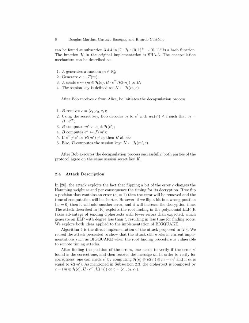
2.4 Attack Description

In [20], the attack exploits the fact that flipping a bit of the error e changes theHamming weight w and per consequence the timing for its decryption. If we flipa position that contains an error (ei = 1) then the error will be removed and thetime of computation will be shorter. However, if we flip a bit in a wrong position(ei = 0) then it will add another error, and it will increase the decryption time.The attack described in [10] exploits the root finding in the polynomial ELP. Ittakes advantage of sending ciphertexts with fewer errors than expected, whichgenerate an ELP with degree less than t, resulting in less time for finding roots.We explore both ideas applied to the implementation of BIGQUAKE.

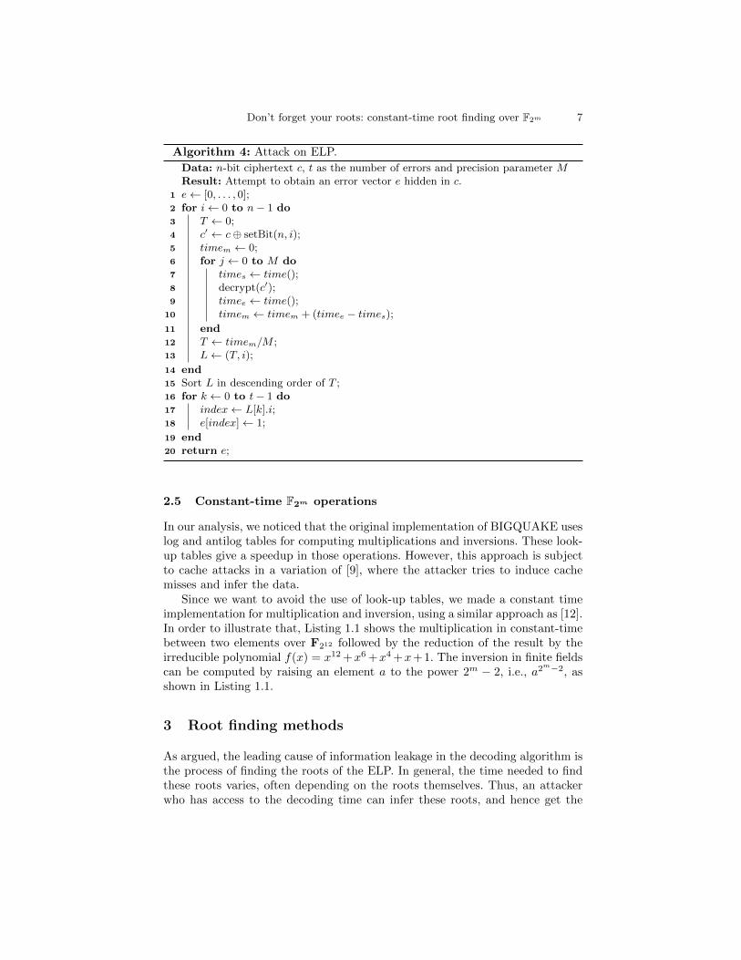
Algorithm 4 is the direct implementation of the attack proposed in [20]. Wereused the attack presented to show that the attack still works in current imple-mentations such as BIGQUAKE when the root finding procedure is vulnerableto remote timing attacks.

After finding the position of the errors, one needs to verify if the error e′

found is the correct one, and then recover the message m. In order to verify forcorrectness, one can check e′ by computing H(e)⊕H(e′)⊕m = m′ and if c3 isequal to H(m′). As mentioned in Subsection 2.3, the ciphertext is composed byc = (m⊕H(e), H · eT ,H(m)) or c = (c1, c2, c3).


Algorithm 4: Attack on ELP.

Data: n-bit ciphertext c, t as the number of errors and precision parameter MResult: Attempt to obtain an error vector e hidden in c.

1 e← [0, . . . , 0];2 for i← 0 to n− 1 do3 T ← 0;4 c′ ← c⊕ setBit(n, i);5 timem ← 0;6 for j ← 0 to M do7 times ← time();8 decrypt(c′);9 timee ← time();

10 timem ← timem + (timee − times);11 end12 T ← timem/M ;13 L← (T, i);

14 end15 Sort L in descending order of T ;16 for k ← 0 to t− 1 do17 index← L[k].i;18 e[index]← 1;

19 end20 return e;

2.5 Constant-time F2m operations

In our analysis, we noticed that the original implementation of BIGQUAKE useslog and antilog tables for computing multiplications and inversions. These look-up tables give a speedup in those operations. However, this approach is subjectto cache attacks in a variation of [9], where the attacker tries to induce cachemisses and infer the data.

Since we want to avoid the use of look-up tables, we made a constant timeimplementation for multiplication and inversion, using a similar approach as [12].In order to illustrate that, Listing 1.1 shows the multiplication in constant-timebetween two elements over F212 followed by the reduction of the result by theirreducible polynomial f(x) = x12 +x6 +x4 +x+ 1. The inversion in finite fieldscan be computed by raising an element a to the power 2m − 2, i.e., a2m−2, asshown in Listing 1.1.

3 Root finding methods

As argued, the leading cause of information leakage in the decoding algorithm isthe process of finding the roots of the ELP. In general, the time needed to findthese roots varies, often depending on the roots themselves. Thus, an attackerwho has access to the decoding time can infer these roots, and hence get the


vector of errors e. Next, we propose modifications in four of these algorithms toavoid the attack presented in Subsection 2.4.

Strenzke [21] presents an algorithm analysis for fast and secure root findingfor code-based cryptosystems. He uses as a basis for his results the implemen-tation of “Hymes ” [7]. Some of that implementation uses, for instance, log andantilog tables for some operations in finite fields, which are known to be vulner-able. Given that, we rewrote those operations without tables and analyzed eachline of code from the original implementations, taking care of modifying themin order to eliminate processing that could indicate root-dependent executiontime. The adjustments were made in the following algorithms to find roots: ex-haustive search, linearized polynomials, Berlekamp trace algorithm (BTA), andsuccessive resultant algorithm (SRA).

In this work, we use the following notation: given a univariate polynomial f ,with degree d and coefficients over Fpn , one needs to find its roots. In our case,we are concerned about binary fields, i.e., p = 2. Additionally, we assume thatall the factors of f are linear and distinct.

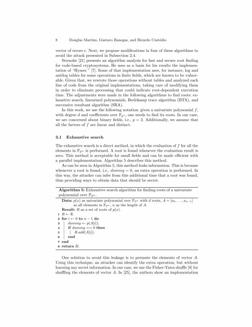
3.1 Exhaustive search

The exhaustive search is a direct method, in which the evaluation of f for all theelements in F2m is performed. A root is found whenever the evaluation result iszero. This method is acceptable for small fields and can be made efficient witha parallel implementation. Algorithm 5 describes this method.

As can be seen in Algorithm 5, this method leaks information. This is becausewhenever a root is found, i.e., dummy = 0, an extra operation is performed. Inthis way, the attacker can infer from this additional time that a root was found,thus providing ways to obtain data that should be secret.

Algorithm 5: Exhaustive search algorithm for finding roots of a univariatepolynomial over F2m .

Data: p(x) as univariate polynomial over F2m with d roots, A = [a0, . . . , an−1]as all elements in F2m , n as the length of A.

Result: R as a set of roots of p(x).1 R← ∅;2 for i← 0 to n− 1 do3 dummy ← p(A[i]);4 if dummy == 0 then5 R.add(A[i]);6 end

7 end8 return R;

One solution to avoid this leakage is to permute the elements of vector A.Using this technique, an attacker can identify the extra operation, but withoutlearning any secret information. In our case, we use the Fisher-Yates shuffle [8] forshuffling the elements of vector A. In [25], the authors show an implementation


of the shuffling algorithm safe against timing attacks. Algorithm 6 shows thepermutation of the elements and the computation of the roots.

Algorithm 6: Exhaustive search algorithm with a countermeasure for find-ing roots of an univariate polynomial over F2m .

Data: p(x) as a univariate polynomial over F2m with d roots,A = [a0, . . . , an−1] as all elements in F2m , n as the length of A.

Result: R as a set of roots of p(x).1 permute(A);2 R← ∅;3 for i← 0 to n− 1 do4 dummy ← p(A[i]);5 if dummy == 0 then6 R.add(A[i]);7 end

8 end9 return R;

Using this approach, we add one extra step to the algorithm. However, thispermutation blurs the sensitive information of the algorithm, making the usageof Algorithm 6 slightly harder for the attacker to acquire timing leakage.

The main costs for Algorithm 5 and Algorithm 6 are the polynomial evalua-tion and we define as Cpol eval. Since we need to evaluate each element in A, itis safer to assume that the total cost is:

Cexh = n(Cpol eval). (4)

We can go further and express the cost for one polynomial evaluation bythe number of operations in finite fields. In our implementation4 the cost isdetermined by the degree d of the polynomial and basic finite field operationssuch as addition and multiplication. As a result, the cost for one polynomialevaluation is:

Cpol eval = d(Cgf add + Cgf mul). (5)

3.2 Linearized polynomials

The second countermeasure proposed is based on linearized polynomials. Theauthors in [14] propose a method to compute the roots of a polynomial over F2m ,using a particular class of polynomials, called linearized polynomials. In [21],this approach is a recursive algorithm which the author calls “dcmp-rf”. Inour solution, however, we present an iterative algorithm. We define linearizedpolynomials as follows:

4 available in https://git.dags-project.org/gustavo/roots finding


Definition 2. A polynomial `(y) over F2m is called a linearized polynomial if

`(y) =∑i

ciy2i

, (6)

where ci ∈ F2m .

In addition, from [24], we have Lemma 1 that describes the main property oflinearized polynomials for finding roots.

Lemma 1. Let y ∈ F2m and let α0, α1, . . . , αm−1 be a standard basis over F2.If

y =

m−1∑k=0

ykαk, yk ∈ F2 (7)

and `(y) =∑j cjy

2j

, then

`(y) =

m−1∑k=0

yk`(αk). (8)

We call A(y) over F2m as an affine polynomial if A(y) = `(y)+β for β ∈ F2m ,where `(y) is a linearized polynomial.

We can illustrate a toy example to understand the idea behind finding rootsusing linearized polynomials.

Example 1. Let us consider the polynomial f(y) = y2 +(α2 +1)y+(α2 +α+1)y0

over F23 and α are elements in F2[x]/x3 + x2 + 1. Since we are trying to findroots, we can write f(y) as

y2 + (α2 + 1)y + (α2 + α+ 1)y0 = 0

ory2 + (α2 + 1)y = (α2 + α+ 1)y0 (9)

We can point that on the left hand side of Equation 9, `(y) = y2 + (α2 + 1)y isa linearized polynomial over F23 and Equation 9 can be expressed just as

`(y) = α2 + α+ 1 (10)

If y = y2α2 + y1α+ y0 ∈ F23 then, according to Lemma 1, Equation 10 becomes

y2`(α2) + y1`(α) + y0`(α

0) = α2 + α+ 1 (11)

We can compute `(α0), `(α) and `(α2) using the left hand side of Equation 9and we have the following values

`(α0) = (α0)2 + (α2 + 1)(α0) = α2 + 1 + 1 = α2

`(α) = (α)2 + (α2 + 1)(α) = α2 + α2 + α+ 1 = α+ 1

`(α2) = (α2)2 + (α2 + 1)(α2) = α4 + α4 + α2 = α2.

(12)


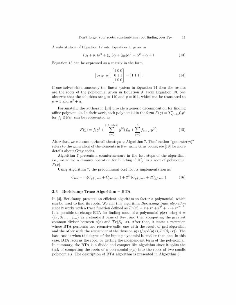
A substitution of Equation 12 into Equation 11 gives us

(y2 + y0)α2 + (y1)α+ (y0)α0 = α2 + α+ 1 (13)

Equation 13 can be expressed as a matrix in the form

[y2 y1 y0

] 1 0 00 1 11 0 0

=[1 1 1

]. (14)

If one solves simultaneously the linear system in Equation 14 then the resultsare the roots of the polynomial given in Equation 9. From Equation 13, oneobserves that the solutions are y = 110 and y = 011, which can be translated toα+ 1 and α2 + α.

Fortunately, the authors in [14] provide a generic decomposition for findingaffine polynomials. In their work, each polynomial in the form F (y) =

∑tj=0 fjy

j

for fj ∈ F2m can be represented as

F (y) = f3y3 +

d(t−4)/5e∑i=0

y5i(f5i +

3∑j=0

f5i+2jy2j

) (15)

After that, we can summarize all the steps as Algorithm 7. The function “generate(m)”refers to the generation of the elements in F2m using Gray codes, see [19] for moredetails about Gray codes.

Algorithm 7 presents a countermeasure in the last steps of the algorithm,i.e., we added a dummy operation for blinding if X[j] is a root of polynomialF (x).

Using Algorithm 7, the predominant cost for its implementation is:

Clin = m(Cgf pow + Cpol eval) + 2m(Cgf pow + 2Cgf mul) (16)

3.3 Berlekamp Trace Algorithm – BTA

In [4], Berlekamp presents an efficient algorithm to factor a polynomial, whichcan be used to find its roots. We call this algorithm Berlekamp trace algorithmsince it works with a trace function defined as Tr(x) = x+x2 +x22

+ · · ·+x2m−1

.It is possible to change BTA for finding roots of a polynomial p(x) using β ={β1, β2, . . . , βm} as a standard basis of F2m , and then computing the greatestcommon divisor between p(x) and Tr(β0 · x). After that, it starts a recursionwhere BTA performs two recursive calls; one with the result of gcd algorithmand the other with the remainder of the division p(x)/ gcd(p(x), T r(βi ·x)). Thebase case is when the degree of the input polynomial is smaller than one. In thiscase, BTA returns the root, by getting the independent term of the polynomial.In summary, the BTA is a divide and conquer like algorithm since it splits thetask of computing the roots of a polynomial p(x) into the roots of two smallspolynomials. The description of BTA algorithm is presented in Algorithm 8.


Algorithm 7: Linearized polynomials for finding roots over F2m .

Data: F (x) as a univariate polynomial over F2m with degree t and m as theextension field degree.

Result: R as a set of roots of p(x).1 `ki ← ∅; ìs ← ∅; Ajk ← ∅; R← ∅; dummy ← ∅;2 if f0 == 0 then3 R.append(0);4 end5 for i← 0 to d(t− 4)/5e do6 ì(x)← 0;7 for j ← 0 to 3 do

8 ì(x)← ì(x) + f5i+2jx2j ;

9 end10 ìs[i]← ì(x);

11 end12 for k ← 0 to m− 1 do13 for i← 0 to d(t− 4)/5e do14 `ki ← ìs(α

k);15 end

16 end17 A0

i ← ∅;18 for i← 0 to d(t− 4)/5e do19 A0

i ← f5i;20 end21 X ← generate(m);22 for j ← 1 to 2m − 1 do23 for i← 0 to d(t− 4)/5e do24 A← Aj−1

i ;

25 A← A+ `δ(X[j],X[j−1])i ;

26 Aji ← A;

27 end

28 end29 for j ← 1 to 2m − 1 do30 result← 0;31 for i← 0 to d(t− 4)/5e do32 result = result+ (X[j])5iAji ;33 end34 eval = result+ f3(X[j])3;35 if eval == 0 then36 R.append(X[j]);37 else38 dummy.append(X[j]);39 end

40 end41 return R;


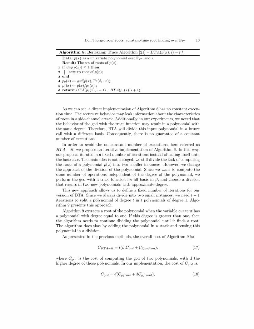
Algorithm 8: Berlekamp Trace Algorithm [21] – BTA(p(x), i)− rf .

Data: p(x) as a univariate polynomial over F2m and i.Result: The set of roots of p(x).

1 if deg(p(x)) ≤ 1 then2 return root of p(x);3 end4 p0(x)← gcd(p(x), T r(βi · x));5 p1(x)← p(x)/p0(x) ;6 return BTA(p0(x), i+ 1) ∪BTA(p1(x), i+ 1);

As we can see, a direct implementation of Algorithm 8 has no constant execu-tion time. The recursive behavior may leak information about the characteristicsof roots in a side-channel attack. Additionally, in our experiments, we noted thatthe behavior of the gcd with the trace function may result in a polynomial withthe same degree. Therefore, BTA will divide this input polynomial in a futurecall with a different basis. Consequently, there is no guarantee of a constantnumber of executions.

In order to avoid the nonconstant number of executions, here referred asBTA− it, we propose an iterative implementation of Algorithm 8. In this way,our proposal iterates in a fixed number of iterations instead of calling itself untilthe base case. The main idea is not changed; we still divide the task of computingthe roots of a polynomial p(x) into two smaller instances. However, we changethe approach of the division of the polynomial. Since we want to compute thesame number of operations independent of the degree of the polynomial, weperform the gcd with a trace function for all basis in β, and choose a divisionthat results in two new polynomials with approximate degree.

This new approach allows us to define a fixed number of iterations for ourversion of BTA. Since we always divide into two small instances, we need t− 1iterations to split a polynomial of degree t in t polynomials of degree 1. Algo-rithm 9 presents this approach.

Algorithm 9 extracts a root of the polynomial when the variable current hasa polynomial with degree equal to one. If this degree is greater than one, thenthe algorithm needs to continue dividing the polynomial until it finds a root.The algorithm does that by adding the polynomial in a stack and reusing thispolynomial in a division.

As presented in the previous methods, the overall cost of Algorithm 9 is:

CBTA−it = t(mCgcd + CQuoRem). (17)

where Cgcd is the cost of computing the gcd of two polynomials, with d thehigher degree of those polynomials. In our implementation, the cost of Cgcd is:

Cgcd = d(Cgf inv + 3Cgf mul), (18)


Algorithm 9: Iterative Berlekamp Trace Algorithm – BTA(p(x))− it.Data: p(x) as an univariate polynomial over F2m , t as number of expected

roots.Result: The set of roots of p(x).

1 g ← {p(x)}; // The set of polynomials to be computed

2 for k ← 0 to t do3 current = g.pop();4 Compute candidates = gcd(current, Tr(βi · x)) ∀ βi ∈ β;5 Select p0 ∈ candidates such as p0.degree ' current

2;

6 p1(x)← current/p0(x) ;7 if p0.degree == 1 then8 R.add(root of p0)9 end

10 else11 g.add(p0);12 end13 if p1.degree == 1 then14 R.add(root of p1)15 end16 else17 g.add(p1);18 end

19 end20 return R

and CQuoRem is the cost for computing the quotient and remainder between twopolynomials. The cost for this computation is:

CQuoRem = d(Cgf inv + (d+ 1)Cgf mul + Cgf add). (19)

3.4 Successive Resultant Algorithm

In [18], the authors present an alternative method for finding roots in Fpm . Lateron, the authors better explain the method in [13]. The Successive ResultantAlgorithm (SRA) relies on the fact that it is possible to find roots exploitingproperties of an ordered set of rational mappings.

Given a polynomial f of degree d and a sequence of rational maps K1, . . . ,Kt,the algorithm computes finite sequences of length j ≤ t+ 1 obtained by succes-sively transforming the roots of f by applying the rational maps. The algorithmis as follows: Let {v1, . . . , vm} be an arbitrary basis of Fpm over Fp, then it ispossible to define m+ 1 functions `0, `1, . . . , `m from Fpm to Fpm such that

`0(z) = z`1(z) =

∏i∈Fp

`0(z − iv1)

`2(z) =∏i∈Fp

`1(z − iv2)

· · ·`m(z) =

∏i∈Fp

`m−1(z − ivm)


The functions `j are examples of linearized polynomials, as previously definedin subsection 3.2. Our next step is to present the theorems from [18]. Checkoriginal work for the proofs.

Theorem 1. a) Each polynomial ì is split and its roots are all elements of thevector space generated by {v1, . . . , vi}. In particular, we have `n(z) = zp

m−z.b) We have ì(z) = ì−1(z)p − aiì−1(z) where a := (ì−1(vi))

p−1.c) If we identify Fpm with the vector space (Fp)m, then each ì is a p-to-1 linear

map of ì−1(z) and a pi to 1 linear map of z.

From Theorem 1 and its properties, we can reach the following polynomialsystem:

f(x1) = 0xpj = ajxj = xj+1 j = 1, . . . ,m− 1

xpn − anxn = 0(20)

where the ai ∈ Fpn are defined as in Theorem 1. Any solution of this systemprovides us with a root of f by the first equation, and the n last equationstogether imply this root belongs to Fpn . From this system of equations, [18]derives Theorem 2.

Theorem 2. Let (x1, x2, . . . , xm) be a solution of the equations in Equation 20.Then x1 ∈ Fpm is a solution of f . Conversely, given a solution x1 ∈ Fpm of f ,we can reconstruct a solution of all equations in Equation 20 by setting x2 =xp1 − a1x1, etc.

In [18], the authors present an algorithm for solving the system in Equation 20using resultants. The solutions of the system are the roots of polynomial f(x).We implemented the method presented in [18] using SAGE Math [23] due to thelack of libraries in C that work with multivariate polynomials over finite fields.It is worth remarking that this algorithm is almost constant-time and hence wejust need to protect the branches presented on it. The countermeasure adoptedwas to add dummy operations, as presented in Subsection 3.2.

4 Comparison

In this section, we present the results of the execution of each of the methodspresented in Section 3. We used an Intel® Core(TM) i5-5300U CPU @ 2.30GHz.The code was compiled with GCC version 8.3.0 and the following compilationflags “-O3 -g3 -Wall -march=native -mtune=native -fomit-frame-pointer -ffast-math”. We ran 100 times the code and got the average number of cycles. Table 1shows the number of cycles of root finding methods without countermeasures,while Table 2 shows the number of cycles when there is a countermeasure. Inboth cases, we used d = {55, 65, 100} where d is the number of roots. We remarkthat the operations in the tables are over F212 and F216 . We used two differentfinite fields for showing the generality of our implementations and the costs fora small field and a larger field.


Nr. Roots Field Exhaustive Search Linearized polynomials BTA-rf SRA

55F212 10.152 45.697 9.801 2, 301.663F216 117.307 425.494 72.766 2, 333.519

65F212 12.103 56.270 11.933 2, 711.318F216 139.506 522.208 80.687 2, 782.838

100F212 18.994 84.076 17.322 3, 555.221F216 213.503 863.063 133.487 3, 735.954

Table 1: Number of cycles divided by 106 for each method of finding roots withoutcountermeasures.

Nr. Roots Field Exhaustive Search Linearized polynomials BTA-it SRA

55F212 11.741 45.467 11.489 2, 410.410F216 142.774 433.645 75.467 2, 660.052

65F212 13.497 55.908 14.864 2, 855.899F216 164.951 533.946 86.869 2, 929.608

100F212 20.287 89.118 20.215 4.211.459F216 238.950 882.101 138.956 4, 212.493

Table 2: Number of cycles divided by 106 for each method of finding roots withcountermeasures.

Figure 1 shows the number of cycles for random polynomials with degree 55,65 and 100 and all the operations are over F216 . Figure 1a shows a time vari-ation in the execution time of the exhaustive method, as expected, the averagetime was increased. In 1b, note a variation of time when we did not add thecountermeasures, but when we add them, we see a constant behavior. In 1c, itis possible to see a nonconstant behavior of BTA− rf . However, this is differentfor BTA− it, which shows a constant behavior.

The main focus of our proposal was to find alternatives to compute roots ofELP that has constant execution time. Figure 2 presents an overview betweenthe original implementations and the implementations with countermeasures. Itis possible that when a countermeasure is present on Linearized and on BTA ap-proach, the number of cycles increases. However, the variance of time decreases.Additionally, Figure 2 shows an improvement in time variance for SCA method,without a huge increase on the average time. We remark that the “points” outof range can be ignored since we did not run the code under a separated environ-ment, and as such it could be that some process in our environment influencedthe result.


(a) Comparison between exhaustive searchwith and without countermeasures.

(b) Comparison between linearized polyno-mials with and without countermeasures.

(c) Comparison between BTA-rf andBTA-it executions.

(d) Comparison between SRA and SafeSRA executions.

Fig. 1: Plots of measurements cycles for methods presented in Section 3. Ourevaluation of SRA was made using a Python implementation and cycles mea-surement with C. In our tests, the drawback of calling a Python module from Chas behavior bordering to constant.

6.38 · 108 6.4 · 108 6.42 · 108 6.44 · 108 6.46 · 108

OursLin.

5.24 · 109 5.28 · 109 5.32 · 109 5.36 · 109

OursSCA

7.6 · 108 8 · 108 8.4 · 108 8.8 · 108 9.2 · 108

OursBTA

Fig. 2: Comparison of original implementation and our proposal for Linearized,Successive resultant algorithm and Berlekamp trace algorithm with t = 100.


5 Conclusion

In our study, we demonstrated countermeasures that can be used to avoid remotetiming attacks. In our empirical analysis, i.e, the results in Table 2, BTA-itshows an advantage in the number of cycles which makes it a more efficient andsafer choice. However, the exhaustive search with shuffling shows the smallestvariation of time, which can be an alternative for usage. Still, the problem forthis method is that if the field is large, then it becomes costly to shuffle anditerate all elements.

5.1 Open problems

We bring to the attention of the reader that we did not use any optimization inour implementations, i.e., we did not use vectorization or bit slicing techniquesor any specific instructions such as Intel® IPP Cryptography for finite fieldarithmetic in our code. Therefore, these techniques and instructions can improvethe finite fields operations and speed up our algorithms.

We remark that for achieving a safer implementation, one needs to improvethe security analysis, by removing conditional memory access and protectingmemory access of instructions. Moreover, one can analyze the security of theimplementations, by considering different attack scenarios and performing anin-depth analysis of hardware side-channel attacks.

6 Acknowledgments

We want to thank the reviewers for the thoughtful comments on this work. Wewould also like to thank Tanja Lange for her valuable feedback. We want toextend the acknowledgments to Sonia Belaıd from Cryptoexperts for the discus-sions about timing attacks.

References

1. Banegas, G., Barreto, P.S., Boidje, B.O., Cayrel, P.L., Dione, G.N., Gaj, K., Gu-eye, C.T., Haeussler, R., Klamti, J.B., Ndiaye, O., Nguyen, D.T., Persichetti, E.,Ricardini, J.E.: DAGS: Key encapsulation using dyadic GS codes. Journal of Math-ematical Cryptology 12(4), 221–239 (2018)

2. Bardet, M., Barelli, E., Blazy, O., Torres, R.C., Couvreur, A., Gaborit, P., Otmani,A., Sendrier, N., Jean-Pierre, T.: BIG QUAKE BInary Goppa QUAsi–cyclic KeyEncapsulation. Tech. rep., National Institute of Standards and Technology (NIST)(2017)

3. Berlekamp, E.: Algebraic coding theory. World Scientific (2015)4. Berlekamp, E.R.: Factoring polynomials over large finite fields. Mathematics of

computation 24(111), 713–735 (1970)5. Bernstein, D.J.: Cache-timing attacks on AES (2005),

https://cr.yp.to/antiforgery/cachetiming-20050414.pdf


6. Bernstein, D.J., Persichetti, E.: Towards KEM unification. Cryptology ePrintArchive, Report 2018/526 (2018), https://eprint.iacr.org/2018/526

7. Biswas, B., Sendrier, N.: HyMES - an open source imple-mentation of the McEliece cryptosystem (2008), http://www-rocq.inria.fr/secret/CBCrypto/index.php?pg=hyme

8. Black, P.E.: Fisher-Yates shuffle. Dictionary of algorithms and data structures 19(2005)

9. Bruinderink, L.G., Hulsing, A., Lange, T., Yarom, Y.: Flush, gauss, and reload -A cache attack on the BLISS lattice-based signature scheme. In: CryptographicHardware and Embedded Systems - CHES 2016 - 18th International Conference,Santa Barbara, CA, USA, August 17-19, 2016, Proceedings. pp. 323–345 (2016).https://doi.org/10.1007/978-3-662-53140-2 16

10. Bucerzan, D., Cayrel, P.L., Dragoi, V., Richmond, T.: Improved timing attacksagainst the secret permutation in the McEliece PKC. International Journal ofComputers Communications & Control 12(1), 7–25 (2017)

11. Chor, B., Rivest, R.L.: A knapsack-type public key cryptosystem based on arith-metic in finite fields. IEEE Transactions on Information Theory 34(5), 901–909(1988)

12. Chou, T.: Mcbits revisited. In: Cryptographic Hardware and Embedded Systems- CHES 2017 - 19th International Conference, Taipei, Taiwan, September 25-28,2017, Proceedings. pp. 213–231 (2017). https://doi.org/10.1007/978-3-319-66787-4 11

13. Davenport, J.H., Petit, C., Pring, B.: A Generalised Successive Resultants Algo-rithm. In: Duquesne, S., Petkova-Nikova, S. (eds.) Arithmetic of Finite Fields. pp.105–124. Springer International Publishing, Cham (2016)

14. Fedorenko, S.V., Trifonov, P.V.: Finding roots of polynomials over finite fields.IEEE Transactions on communications 50(11), 1709–1711 (2002)

15. McEliece, R.J.: A Public-Key Cryptosystem Based On Algebraic Coding Theory.Deep Space Network Progress Report 44, 114–116 (Jan 1978)

16. Misoczki, R., Barreto, P.S.L.M.: Compact McEliece keys from Goppa codes. In:Selected Areas in Cryptography, 16th Annual International Workshop, SAC 2009,Calgary, Alberta, Canada, August 13-14, 2009, Revised Selected Papers. pp. 376–392 (2009). https://doi.org/10.1007/978-3-642-05445-7 24

17. Patterson, N.: The algebraic decoding of Goppa codes. IEEE Transactions on In-formation Theory 21(2), 203–207 (1975)

18. Petit, C.: Finding roots in GF(pn) with the successive resultant algorithm. IACRCryptology ePrint Archive 2014, 506 (2014)

19. Savage, C.: A survey of combinatorial Gray codes. SIAM review 39(4), 605–629(1997)

20. Shoufan, A., Strenzke, F., Molter, H.G., Stottinger, M.: A timing attack againstpatterson algorithm in the McEliece PKC. In: Information, Security and Cryp-tology - ICISC 2009, 12th International Conference, Seoul, Korea, December 2-4,2009, Revised Selected Papers. pp. 161–175 (2009). https://doi.org/10.1007/978-3-642-14423-3 12

21. Strenzke, F.: Fast and secure root finding for code-based cryptosystems. In:Cryptology and Network Security, 11th International Conference, CANS 2012,Darmstadt, Germany, December 12-14, 2012. Proceedings. pp. 232–246 (2012).https://doi.org/10.1007/978-3-642-35404-5 18

22. Strenzke, F.: Efficiency and implementation security of code-based cryptosystems.Ph.D. thesis, Technische Universitat (2013)


23. The Sage Developers: SageMath, the Sage Mathematics Software System (Version8.7) (2019), https://www.sagemath.org

24. Truong, T.K., Jeng, J.H., Reed, I.S.: Fast algorithm for computing the roots of errorlocator polynomials up to degree 11 in Reed-Solomon decoders. IEEE Transactionson Communications 49(5), 779–783 (2001)

25. Wang, W., Szefer, J., Niederhagen, R.: FPGA-based Niederreiter cryptosystemusing binary goppa codes. In: Post-Quantum Cryptography - 9th InternationalConference, PQCrypto 2018, Fort Lauderdale, FL, USA, April 9-11, 2018, Pro-ceedings. pp. 77–98 (2018). https://doi.org/10.1007/978-3-319-79063-3 4

A Implementation Code

#inc lude <s t d i n t . h>typede f u i n t 1 6 t g f ;g f gf q m mult ( g f in0 , g f in1 ) {

u i n t 6 4 t i , tmp , t0 = in0 , t1 = in1 ;// M u l t i p l i c a t i o ntmp = t0 ∗ ( t1 & 1) ;f o r ( i = 1 ; i < 12 ; i++)

tmp ˆ= ( t0 ∗ ( t1 & (1 << i ) ) ) ;// reduct i ontmp = tmp & 0x7FFFFF ;// f i r s t s tep o f r educt iong f r educt ion = (tmp >> 12) ;tmp = tmp & 0xFFF ;tmp = tmp ˆ ( reduct ion << 6) ;tmp = tmp ˆ ( reduct ion << 4) ;tmp = tmp ˆ reduct ion << 1 ;tmp = tmp ˆ reduct ion ;// second step o f r educt ionreduct ion = (tmp >> 12) ;tmp = tmp ˆ ( reduct ion << 6) ;tmp = tmp ˆ ( reduct ion << 4) ;tmp = tmp ˆ reduct ion << 1 ;tmp = tmp ˆ reduct ion ;tmp = tmp & 0xFFF ;re turn tmp ;

}g f g f i n v ( g f in ) {

g f tmp 11 = 0 ;g f tmp 1111 = 0 ;g f out = in ;out = g f s q ( out ) ; //aˆ2tmp 11 = gf mult ( out , in ) ; //aˆ2∗a = aˆ3out = g f s q ( tmp 11 ) ; // ( a ˆ3) ˆ2 = aˆ6out = g f s q ( out ) ; // ( a ˆ6) ˆ2 = aˆ12tmp 1111 = gf mult ( out , tmp 11 ) ; //aˆ12∗aˆ3 = aˆ15out = g f s q ( tmp 1111 ) ; // ( a ˆ15) ˆ2 = aˆ30out = g f s q ( out ) ; // ( a ˆ30) ˆ2 = aˆ60out = g f s q ( out ) ; // ( a ˆ60) ˆ2 = aˆ120out = g f s q ( out ) ; // ( a ˆ120) ˆ2 = aˆ240out = gf mult ( out , tmp 1111 ) ; //aˆ240∗aˆ15 = aˆ255out = g f s q ( out ) ; // ( a ˆ255) ˆ2 = 510out = g f s q ( out ) ; // ( a ˆ510) ˆ2 = 1020out = gf mult ( out , tmp 11 ) ; //aˆ1020∗aˆ3 = 1023out = g f s q ( out ) ; // ( a ˆ1023) ˆ2 = 2046out = gf mult ( out , in ) ; //aˆ2046∗a = 2047out = g f s q ( out ) ; // ( a ˆ2047) ˆ2 = 4094return out ;

}

Listing 1.1: Multiplication of two elements in F212 and inversion of an elementin F212

don’t forget your roots: constant-time root nding …don’t forget your roots: constant-time root...

Documents