DEPARTMENT OF PLANS AND PROGRAMSMACROECONOMIC POLICY DIVISIÓN

APPENDICES TO THE DOMINICAN REPUBLIC

MACROECONOMIC ASSESSMENT PAPER, 1993

APPENDICES

Appendix I.

Appendix II.

Appendix III

Appendix IV

Appendix V.

Flow of Funds Framework for a Privately-led CurrentAccount Déficit.

Real Wages and the Inflation Tax.

Decomposition of Nominal Interest Rates and Spreads inThe Dominican Republic: A Simple Framework.

Effects of High Interest Rates and of StructuralAdjustment on the Solvency of the Banking Sector.

Endogenous Growth:Dominican Republic.

Rationale and Sources in the

APPENDIX I

The Flow of Funds Framework For a Privately Led Current Account Déficit.

This Appendix describes the elementary arithmetíc of the financing ofcurrent account, discussed in Section II-B.3 of the report. Inparticular, it illustrates the difference between prívate -capital flowsthat finance a current account déficit and those that finance a change inthe quantity of money. The framework is kept at the simplest possiblelevel.

It is considered that there are two Consolidated sectors: the"government", which includes both the central government and the centralbank and the "private sector" that includes the banking system. It isalso assumed that the central bank fixes the exchange rate and follows astrict "convertibility" policy (i.e., creating money only through thepurchase of foreign exchange). In addition, the economy is assumed to besmall, with all goods being internationally traded. Then, the nominalexchange rate becomes the international price level, the inflation rate isassumed at zero, and the distinction between nominal and real magnitudesbecomes unnecessary. For added simplicity, it is assumed the case of anon-growing economy.

At every period, the government budget constraint is

[1] g + rf - t = Af + Am

where g is government expenditures in goods and services, f the stock ofnet foreign liabilities held by government, r is the real world interestrate, t are taxes, and m the stock of real money. The symbol A, asusual, represents the change between the beginning and the end of theperiod.

The budget constraint of the private sector, in turn, is

[2] e + ra - (y-t) = Aa - Ara

where a are private net foreign liabilities, y is income (product), ande are private expenditures.

Notice that these two expressions tell a very similar story: In equation[1] the excess of public expenditure - including payments of interest onthe debt - over income is financed by either an increase in the foreignpublic debt or else by the issuance of money. In equation [2], the excessof private expenditure - including payments of interest on the debt - overdisposable income is financed by the accumulation of foreign private debtin excess of the increase in the demand for money. Notice also that thestock of foreign liabilities (f and a) would be negative in the case ofassets.

If these two expressions are merged together, they yield

[3] Ai + Aa = g + e + rf+ ra - y

which is the economy's budget constraint or the balance of paymentsidentity. Thus the balance of payments is equal to the sum of the prívatesector's and the public sector's budgets.

Equilibrium in the market for commodities requires the total supply ofcommoditles (i.e., the sum of commodities produced, y, plus commoditiesimported) be equal to the total demand (i.e. , the sum of the domesticdemand for commodities by the private sector, e, and by government, g,plus commodities exported). Since exports minus imports is equal to thebalance of trade. T, then equilibrium requires

14] **'.-*-,.••

so that the balance of payments can be written as

[5] Af + Aa - fr + ar - T

Where the right hand side of [5] is the current account balance (CA)

CA = rf + ra - T

Expression [5] is useful to highlight the fact that, for a country. anexcess of expenditures including interest payments on the debt, overincome can be financed only by an increase in the foreign debt ( or elseby a depletion of International reserves) of either the government or theprivate sector.

Of course, all these relationships (except the condition for equilibriumin the market for commodities [4]) are identities, and say nothing aboutbehavior. But they are still useful for characterizing several differentpossibilities . Consider the private sector constraint [2], and therelationship between: changes in foreign private liabilities, Aa; changesin the real money stock; Am, and change in the level of expenditures, e.In particular, suppose that for a certain period we observe borrowing fromabroad,1 i. e., a term Aa > 0. For a given level of income and taxes , thiscould be generated by either (i) a transitory rise in privateexpenditures, e, or (ii) a desire to accumulate real cash balances,Am > 0. In the first case, the real money stock does not change, i. e.,Am = O, and nothing changes in the government budget constraint. At theend of the period, the level of the debt, a, would be higher, and thiswill require that the private sector repay the debt through a permanentlower level of expenditures 2, but this may not necessarily involve

_

1 This could be in the form of autonomous " capital inflows" drawn by highinterest rates or else the contracting of loans abroad by the private sector.

2 Unless the higher current expenditures are in productive investments andas a result a higher income and expenditures result.

government in any way. In case (ii), in whích the capital ínflow is usedto accumulate real money, i.e., Aa = A/n, some terms in the governmentbudget constraint are affected: the public transfers foreign exchange tothe government in exchange for domestic money, and government's (morespecifically, the central bank's) foreign assets increase. In terms of theoverall balance of payments expression [4] , this is a simple "switch" fromprivate to government foreign assets (i.e., from a to f). '

Three features that characterize the current macroeconomic framework ofthe DR are: (i) a surplus of 1.6% of GDP in the public sector's budget in1992, (ii) a big jump in the current account déficit from 2.5% of GDP 1991to 6% in 1992, (iii) an increase in the demand of money as evidenced bythe decline in the velocity of broad money from 3.6 in 1991 to 3.1 ín1992. The mechanics of the process leading up to the current accountdéficit can be shown in terms of the simple equations of this Appendix.

The current account déficit originates in the private sector's budget(equation [2]) because the public sector's budget (equation [3]) is insurplus. The excess of private expenditure (e+ra) over private disposableincome (y - t) is not financed by drawing down holdings of real domesticmoney because the demand of money is expanding. Rather external capitalinflows to the private sector are financing both the excess expenditureand the built up of money balances. From equation [1] the combination ofthe public sector surplus and the increase in the demand for money(seignorage) result in a reduction in the external public debt (Af < O ) .In fact this reduction, by itself, works towards a current surplus, ascan be checked in equation [3]. But since this effect is much smallerthan the external borrowing by the private sector (Aa > Af) the finaloutcome is a huge current account déficit.

The two issues regarding the privately led current account déficit aresustainabilty and vulnerability. As to sustainabilty the key questionsare: (i) is the excess of expenditures in consumption or in investment?;(ii) if in investment, will the return be sufficient to repay the debtservice?; and (iií) is the excess of expenditures the result of a one-timeself correcting process or else does it require cool down policy action?.As to vulnerability, the key question is whether the excess expenditurewill be quickly washed out if financing were suddenly withdrawn oralternatively whether the withdrawal will prompt a foreign exchangecrisis.

The data for the DR shows that the 3.5% of GDP deterioration of thecurrent account from 1991 to 1992 is associated with a 2.6% of GDPincrease in investment and a 0.9% increase in total consumption. Thistells us that the process is safe on this account. (However, as noted inthe report; the sectoral distribution of the ratios is worrisome becauseprivate consumption to GDP rose unlike public consumption to GDP whichdropped; in other words, the brunt of the adjustment was borne by publicsavings). The problem is that a significant share of external financingof the current account déficit comes in the form of speculative short termcapital inflows. These are attracted by the very high interest rates

(about 10% real annual) and then on-lent to borrowers at real annual ratesof over 25%. The fact that the financing is short-term poses the questionof vulnerability. In turn, the high lending rates suggest the possibilityof borrowers' default risk and thus the process might not be sustainable.

APPENDIX II

Real Wages and the Inflation Tax.

During the months preceding the enactment of the current stabilizationprogram, the DR experienced extremely high and accelerating levéis ofinflation. As a result of the program, the inflation rate fell almostimmediately.

The parpóse of this Appendix is to show the effect of these inflationrates on real "disposable" wages, thus to underline why nominal wagesdeflated by the consumar price level is an inadequate measure of thepurchasing power of real disposable wages. We provide a crude measurementof both the inflation tax and the welfare costs of inflation for thetypical case of a wage earner who receives a nominal salary at thebeginning of the month and spends it through the month.

It is well known that inflation is a "tax" on cash balances, being thecounterpart of the revenues captured by the monetary authority vía thecreation of money. As any tax, there ís a transfer from the payer (moneyholders, in this case) to the collector (the government) . Also, as in thecase of other taxes, there are net "welfare costs". i. e., a loss tosomebody (the tax payer) which is not a gain to anybody.1 It is also knownthat the inflation tax is highly regressive. Those in the lower incomebrackets have far less possibilities of holding their wealth in otherassets, and hold proportionally more cash balances than those in higherbrackets. It should be emphasized that these costs are unrelated to. andindependent from any deterioration of the real wage due to a lack ofmonthly adjustment to inflation.

Table A2-1 shows the annual inflation rates from July 1990 to March 1991,both for the last 12 months (as it is usually computed) and for the lastmonth (i.e., the annual rate at which prices have been rising during thelast month). The highest level of the latter occurs in August 1990, at a420% annual rate.

Suppose the "demand for money" (i.e., the average of real cash balancesheld through a month), m, is an expression of the form

[1] ñ = (y/2)exp(-aji) ,

where y is real income, it is the monthly inflation rate and a is aparameter, which determines the "semilogarithmic" elasticity of the demandfor money. What [1] shows is simply that, the higher the inflation rate(which is a cost of holding money), the lower the real money stock held bythe public. The higher the coefficient a, the stronger the response ofthe real money stock to the inflation rate. For our purposes, [1] hasbeen written assuming that for an inflation rate of zero the real moneystock held will be equal to half the monthly real income (wage).2

1 This is called sometimes the "deadweight loss" of the tax.i

2 This implies that the wage is spent uniformly through the month.

Table A2-1Annual Inflation Rates from July 1990 to March 1991

(Percent)

Last 12 Months

Last Month

Jul

43

81

Aug

60

420

Sep

67

187

Oct

76

285

Nov

90

264

Dec

100

180

Jan

97

.8

Feb

97

10

Mar

96

20

For a given inflation rate 7t, the inflation tax payment (and governmentrevenue) is the product of real money (the "tax base") times the inflationrate (the "tax rate"), i.e.,

[2] InflTaxPmt= (y/2) exp (-arc) u.

There is, in addition, a "welfare cost", which is raeasured as the áreaunder the demand curve. This represents the costs of performingtransactions with a smaller money stock.3 A crude measurement can be givenby "linearizing" expression [1] and simply taking the difference betweenthe stock and the stock that would prevail with zero inflation, times theinflation rate, divided by two, i.e.,

[3] WelfCost = {[y/2] - [ (y/2) exp (-ajt) ]} JT / 2 .

Charts 1 and 2 show the results of some calculations to illustrate theimportance of the inflation tax and welfare costs on the purchasing powerof real disposable wages. The first is an illustration of the "taxcosts", welfare costs and their sum, for the highest inflation rate of theperiod (420% per year in August 1990), for alternative valúes of theparameter a (from zero to 20). Notice that although higher valúes of amean that less of the inflation tax is payed, but it also means that thewelfare costs of using less money are higher. For the inflation rate of420% per year, the máximum costs is for a zero coefficient a (7.5% of thereal salary). Higher valúes of the parameter decrease the total costs tothe wage earner, but never below 4% of the salary.

Chart 2 calculates the same magnitudes (inflation tax payment, welfarecost and their sum) but taking a given level of the parameter, at a = 5,and plotting different annual inflation rates. Notice that the "taxpayment" is also the revenue received from government, and (as in any

3 For example, the costs of storing consumption goods at home ratherthan performing more frequent purchases.

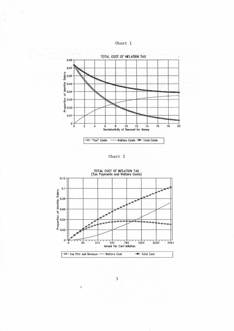
Chart 1

TOTAL COST OF INFLATON TAX0.08

6 8 10 12 U 16SsmiülasHclty of Damand for Money

18 20

"Tax" Costs • Welfare Costs - Told Costs

Chart 2

0.12

0.1

0.08

o3 0.06

~ 0.04

0.02

TOTAL COST OF UFLATION TAX(Tax Poymenís and Welfare Casis)

60 214 435 792 1355Annud Per C«nt Inflotion

2230 3564

• Tax Pml and Reverme • Welfare Cosí • Total Cosí

other tax) there is an inflation rate above which the tax payment (andgovernment revenue) decreases. In our case, of a parameter a = 5, such apoint is at an annual inflation rate of 792% (which is equivalent to 20%per month).

The point highlighted by this exercise is that, during the period ofhighest inflation, the total costs to wage earners (as to any other moneyholders) have been important (probably between 7 and 5 per cent of theirreal salary). The fall in the inflation rate increased the level of realdisposable wages by reducing the inflation tax and the welfare cost ofinflation.

APPENDIX III

Decomposition of Nominal Interest Rates and Spreads in the DominicanRepublic: A Simple Framework.

The high level of bank lending rates in the DR, rL, is made up of twocomponents, a large international spread, s1, between the DR bank depositrate (in DR$) , rB, and the US deposit rate (in US$), rus and a largespread, SH, between DR's lending and deposit rates.

[1]

[2]

The Domestic Spread.

The high domestic spread can partly be accounted for by the 20% non-interest bearing reserve requirement against deposits. With risklessdeposit and lending rates, free entry into the banking industry, and fewintermediation costs, it would be the case that the competitive risk-freelending rate, r, is given by

[3]i-a

Where rB is the risk-free deposit rate and a is the (binding) reserverequirement (non interest-bearing reserves as a fraction of deposits).When a - 0.2, as in the DR, the ratio of lending rate to borrowing ratewould be 1.25 on this count.

Lending rates of course are far from riskless, because of the possibilitythat the borrower might default on the loan. The actual competitivelending rate, r, is therefore the risk-free lending rate plus theborrowers' default risk premium, fi1.1 Thus,

In addition, the banking sector in the DR is far from competitive, so the

1 With risk-neutral banks, the risk premium is obtained from the followingrelationship:

icL=i í(z)f(z) dz+i¿~f(z) dz

Here i1 is the rate of return obtained by the borrower, and f(z) is the densityfunction of i1.

i

actual lendlng rate rL is the sum of the competitiva lending rate and amonopoly premium, ¿i, which includes both excess profits due to monopolyand any x-inefficiency or organizational slack permitted by the absence ofeffective competition.2

[5] r*=rL+i

Summarizing the relationship between the lending and the borrowing ratethus far, we have

[6]X "~c

or

[7]i ¿j

Thus the spread between the lending rate and the risk-free borrowing(deposit) rate can be attributed to: the reserve requirement, theborrowers' default risk premium, and a monopoly premium.

The International Spread.

The DR$ borrowing (deposit) rate can differ from the risk-free US$ depositrate for three reasons.3 Without complete de jure and de facto depositinsurance , deposits are risky. The second is expectations of changes inthe exchange rate. Under uncovered interest parity (ensured by perfectInternational financial market integration, risk neutrality, andstatistical independence of changes in the exchange rate and the rate ofinflation) the Dominican deposit rate would equal the US deposit rate plusthe expected proportional increase in the price of the US $. The third isany difference other than depreciation and default risk, reflectingmarket segmentation; that is , imperfect capital mobility.

Let, é, be the expected proportional rate of depreciation of the Dominicanpeso, 5B the default risk premium on DR$ deposits, m the spread due toInternational market segmentation, and rus the US deposit interest rate.It follows that,

or

2 n also includes the influence of risk aversión, ignored in the note.

3 Dífferential taxation issues are ignored.

Thus the spread between the DR's borrowing (deposit) rate and the risk-free US$ deposit rate can be attributed to combination of three factors:exchange rate devaluations, international market segmentation, and adefault risk premium.

3

APPENDIX IV

Effects of High Interest Rates and Structural Adjustment on theSolvency of the Banking System.

Introduction

As mentioned in the Report, the DR, after the implementation of thestabilization and reform program, continúes to experience both high ex-post real interest rates and high spreads between borrowing and lendingrates. This phenomenon is common to many economies undergoing structuralreforms as well as an important reduction in the inflation rate.

The purpose of thís Appendix is to provide a very simple framework thathelps to explain the mechanism by which transitory shocks can have alasting, persistent and sometimes permanent effect on both lendinginterest rates and the solvency of the banking system. The transitoryshocks that can trigger this mechanism are, precisely, the kind of shocksto which the DR has been subjected, i.e., a rise in the real ex-postborrowing interest rate (due to abrupt disinflation and to the lack ofcertainty about the ultímate success of the stabilization effort) and achange in the structure of relative prices (due to the trade reforms).

The mechanism has a very simple intuitive explanation: shocks thattemporarily reduce the profitability of existing firms forcé firms toborrow beyond the current valué of their net worth. This generates theexistence of liabilties to banks which exceed the firms's net worth, anda higher lending rate charged by banks. Depending on the severity andpersistence of the shock, in some cases this leads to a temporary problem,which is resolved as the firms'profitability is restored, but in others itleads to a situation which is not sustainable in the long run, withlending rates and spreads growing without bound and a threat to thesolvency of the banking system.

In what follows, we first present a very simple framework that formalizesthis mechanism. Then, we proceed to illustrate the different possiblescenarios by means of simulations. It should be stressed that thesesimulations are for illustrative purposes only. although the qualitativeconclusions are applicable to the case of the DR.

A Simple Analytical Framework

We consider the case of the typical firm, with accrued profits at time tbeing defined as

[1] U* * ptx - w-B^rf.!

where xpe are sales (output, x , multiplied by the "real", or relative

price of the product, pt ), w are payments to labor and Bt_^,it-\ are,respectively, the firm's indebtedness and the real interest rate at theend of the previous period (i.e., the beginning of the current period).All variables are expressed in real terms. We assume that profits are

i

distributed if and only if accrued profits defined as in [1] are positiva,and that

[!' ] Be - BM = -U? = w + BM r£j - pex

i. e. , that the firm engages in net borrowing, at every period, by the sameamount of its accrued losses (negative accrued profits) . Thus the typicalfirm increases its indebtedness , when necessary, to pay for its wage bilíand the interest on its previous indebtedness.

If the firm is in a long run equilibrium, its indebtedness is constant,net borrowing is zero and profits will be positive and constant. We alsoassume that in this long run equilibrium real indebtedness is equal to themarket valué of the firm stock of capital, k, which we take to beconstant.

We define "non-performing debt", B1"' , as the difference between debt andthe valué of the typical firm's capital stock, i. e.,

[2] Bf = *,-*,

and assume that commercial banks establish a lending rate that depends onboth the borrowing rate and the proportion of non-performing debt to totaldebt, according to the following expression:

[3] rS-rVB /We'1'""'"

where IL , and IB are the lending and deposit (banks' borrowing) rates , andy is a positive coefficient. For simplicity, and in order to highlight therole of non-performing debt that we are analyzing, we assume that banksprofits are zero, and that there are no costs associated with theoperations of banks . l

Expression [3], that has a simple intuitive explanation, consists of twoparts. The first is the term rg (B/k) , which reflects the fact that if non-performing bank assets cannot be recovered during the period, then theinterest rate charged on loans needs to be sufficiently high so thatinterest on performing assets is sufficient to pay for all loans, i. e.,

[3']

or

[3"] IL = IB (B/k)

1 For simplicity we are ignoring the effect on the spread between theborrowing and lending rate of reserve requirements, operating costs, and any x-ineffeciency. These are discussed in the previous appendix.

which is the first term of [3]. The second term, eT[BJn>M/A:1 , is intended

to reflect aversión to risk by banks, which results in a rate still higherthan the one indicated by the first part of the expression, for y > O .

Expressions [2] and [3] are sufficient to determine the behavior of allthe magnitudes involved (firms'profits, borrowing and indebtedness, non-performing loans, the lending real interest rate and the "spread"),provided we know the behavior of the borrowing rate and the price of theproduct. These are precisely the variables that we will use to motívatevarious plausible scenarios.

Both real deposit rates and relative product prices are magnitudes playingan important role in countries undergoing stabilization programa andstructural reforms, in particular trade reforms, as is the case in the DR.Some 'stylized facts' derived from experience of many episodes can besummarized as follows.

Concerning real deposit rates, there may be a long period in which thoserates may be at high levéis, for various reasons most of which stem fromuncertainty about the success and long-run permanence of the stabilizationand reforms program. These reasons tend to acquire more and moreimportance if reforms to secure the government's long run solvency are notimplemented with the passage of time.

The typical behavior of real deposit rates ís, then, an initial rise. dueto the unexpected fall in the inflation rate (of which a dramatic exampleis the end of 1991 and the beginning of 1992 in the Dominican Republic),a subsequent fall as inflationary expectations start to diminish,counterbalanced sometimes by a tendency to rise if the public does notperceive that lasting fiscal measures are being taken to insure long rungovernment solvency. In order to reflect all these possibilities, in thesimulations that follow we use the following expression to characterizethe path of the monthly real deposits rate:

[4] r*(t) = Cié'"'6 + Cae'"lt + i'B

where Cl, C2, a1 and a2 are coefficients, and r*B is the long run realdeposit rate. The appropriate choice of the coefficients allows tosimúlate a large variety of possible paths of the real deposit rate.

Consider now the role of a structural shock. The first and most importanteffect of a structural reform, foremostly a trade liberalization reform,is a change in relative prices. This, of course, implies losses for someestablished firms and gains for both existing firms and others that havenot being yet established. Therefore, although the portfolio of thebanking system consists of liabilities of all kinds of firms, there willbe an initial dominance by established firms, that at least initially willsuffer losses. Furthermore, we can think of the "typical firm" describedbefore, as one that undertakes all kind of activities (import substitutionand export activities). If this is the case, we can model the temporaryeffects of changes in relative prices as an initial fall in the relative

price of the typical firm, with a recovery that, although concludes witha higher relative price, such recovery takes time.

In a manner formally similar to the case of the real borrowing rate, inthe simulations that follow we use the following general expression tocharacterize the behavior of the relative price of output:

[5] p(t) = D^e-*** + D^-^ +p*

where D1,D2,al and a2 are coefficients, and p* is the long run relativeprice. As in the previous case, a suitable choice of the parametersgenerates plausible paths for the relative price.

The Results of Some Simulations

The "general flavor" of the mechanism

Before we proceed to perform some illustrative simulations, it will beuseful to comment on the intuitive interpretation of the mechanism atwork. As explained before, the element or external shock that triggersthe adjustment can be either changes in the real deposit interest rate orthe relative price of output, or both. In either case, the nature of theadjustment is the same: a transitory fall in the firms'profitability,that eliminates normal profits and requires additional net borrowing forcovering production costs (the wage bilí) and for paying interest on theexisting debt. The accumulation of indebtedness beyond the firms'net worth(i.e., the presence of "non-performing" assets in the banks'portfolio)motivates banks to increase the real lending rate to firms (and thereforethe spread). Since the external shock is transitory, if the magnitude andduration of this higher lending rate is minor then positive accruedprofits reappear and are used to pay for the transitorily higher cost ofcredit, non-performing loans are gradually eliminated and the systemssettles to a long run equilibrium. But if the magnitude and duration isintense enough this will not be possible, and after some time the systemwill embark in a non-stable course, that inevitably leads to a bank crisisand/or the need for government assistance.

In all the simulations used in what follows for illustrating these variouspossibilities, the following valúes of the basic parameters are used:

Monthly real output (x) = 100; monthly wage bilí (w) = 60; monthly longrun profits (U(O') )= 10, real market valué of the firm's capital stock (k)— 9163.83; preexisting annual real borrowing and lending interest rate

(r0* = ig-) - .04 (4 per cent), and preexisting relative price of output

(Po-) - 1.

Additional parameters differ for the various simulations, and areindicated in each case.

The case of interest rate shocks

We report here on the results of simulations in which the motivatingelement is a transitory increase in the real deposit rate, starting attime t = 0. The valué of the parameters used in the simulation are asfollows:

Dl = D2 = O , and p* = p0- = 1 , so that the relative price of output does not

change; y = 0 ; C3 = O, at = -.06, C1 = .00316029, r*D = 0. 00327374 .

First, we consider a case in which the shock is mild enough so that, overtime, firms recover, and the banking system returns to a long run

equilibrium. For this parpóse we specify r£. = 0.8 per month, i.e.,initial "jump" of the real deposit rate from a preexisting level of .04 (4percent per year) to .08 (8 percent per year). Charts 1 to 5 show thebehavior of the most interesting magnitudes. Chart 1 depicts the annualborrowing and lending rates, which makes clear that after the initialshock at time t = O both rates converge back to their initial levéis.Chart 2 describes the path of firms'profits, both accrued and distributed.Accrued (and distributed) pre-shock profits are at a level of 10. As aninitial result of the shock (Chart 1), accrued profits fall toapproximately -20 (i.e., an operating loss of 20), Chart 2, so thatdistributed profits cease. As the lending rate, after the initial shock,falls quickly enough to more than compénsate for the interest on theaccumulated additional debt, smaller and smaller losses take place, andafter approximately 20 months accrued profits reappear. For some time,though, those accrued profits, rather than being distributed, are used todiminish firms'indebtedness. By about 51 months indebtedness has beenbrought back to the firms'net worth, non-performing loans have beeneliminated and profits start to be distributed again. Charts 3 shows theflow of monthly net borrowing (positive or negative). Chart 4 graphs thespread between borrowing and lending annual rates, which increases rapidlyfollowing the shock but is eliminated equally rapidly. Finally Chart 5shows the percentage of non-performing loans.

Consider now the case of a more severe shock, case 2, to the realborrowing interest rate. Here, for the same valué of all otherparameters, except C^ = 0.02516242 we assume that the initial shock to the

annual real borrowing rate is a jump to r£ = 0.4 (40 percent per year).Al though this is an extremely high valué, it is entirely plausible for thekind of abrupt disinflation episodes of the magnitude that recently tookplace in the DR.

Charts 6 through 10 describes the variables. In Chart 6, notice thatalthough the real borrowing rate returns to its long run equilibriumvalué, the real lending rate, which initially also falls, after arelatively long time starts increasing again. This is reflected in thespread depicted in Chart 9. Chart 7 helps to explain this behavior. Afterthe initial fall to a negative level, accrued profits start to recover,but by approximately 60 months the situation is reversed, and from there

Case 1: Small Interest Rate Shock

Figure 1

EX-POSI KAL NTBCST R*TES

Figure 3

FRMS NETBOWOWK5

O 11 14 M 41 10 72 *4. II 104 120

Figure 2

Figure 4

HTEREST 8ATC SPREAD

I U SI

O JIM

0404-

OJK»

Figure 5

PERCENTAGEOFNON-PERTORUMO LO/WS

O 12 24 M 72 14 M 101 120

Case 2: Large Interest Rate Shock

Figure 6

EX-POSI REAL KIEBEST RAIES

Figure 7

FRMS PROFITS

-250-tmwimwWmrIM (fe

Figure 8

FRMS NET BCRMMNG

Figure 9

MTERESr RATE 5PREAO

Figure 10

PERCENTAGE OFNCN-PERTORMHG LOANS

7

on losses start increasing without limit. This is mirrored in Chart 8which depicts the firms'net borrowing. What has happened in this case isthat the intensity of the shock has made impossible for profits toeliminate, over time, indebtedness above the firms' net worth, i.e., toeliminate non-performing loans.

What is remarkable in this case is that for a long time, after the initialeffects of the shock. the problem would seem to be on its way toelimination: the real lending rate and the spread are falling, and so arefirms'losses and net borrowing. After a while, nevertheless, the systemshows to contain the seeds of instability -Chart 15- as the percentage ofnon performing loans increase without bound.

The case of a structural shock

Next, we consider the case where the shock originates in a transitory fallof the relative price of output, resulting, as explained before, from astructural reform that changes relative prices, as in the case of tradeliberalization. We assume that the relative price, after the initialfall, settles at a level above the initial, pre-shock level.

We díscuss the case when the intensity of the shock is sufficient topreclude an equilibrium with banking solvency. We assume no change in the

real borrowing interest rate, which remains at its initial level rB = .04(4 per cent per year) throughout. The rest of the fundamental parametersare as the same level as in the previous simulations, except that now wetake the coefficient y = I, rather than zero. The parameters for thebehavior of the relative price equation [4] are:D! = -0.6, D2 = 0.5, P! = 0.015,P2 = 0.05, and p* = 1.1. The parameters forthe borrowing interest rate, equation [4] are: Cx = C2 = 0.

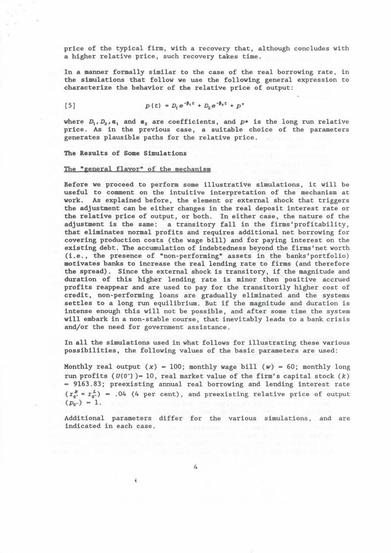
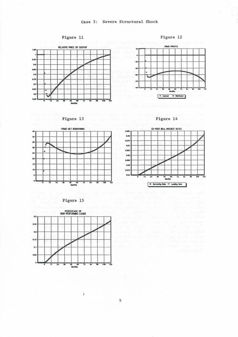
The result of this shock is that although the relative price of outputconverges to an ultímate higher level of 1.1, its transitory fall is deepand prolonged: as shown in Chart 11, it reaches a minimum ofapproximately 0.57 after 7 months and from there on it recovers slowly.Charts 12, 13, and 14, present the behavior of firms' profits and netborrowing very similar to the severe shock in interest rates case, and aconstantly rising level of the real lending interest rate. Notice, inChart 14, that since there is no change in the borrowing rate, thebehavior of the spread can be traced easily from the levéis of the lendingrate. Here again, crisis is inevitable, as witnessed by the secular risein the percentage of non-performing loans (see Chart 15) despite the factthat for some time firms' losses and net borrowing seem to startdiminishing.

Case 3: Severe Structural Shock

Figure 11 Figure 12

WOUTPUT

m

•

V1

y*

X

4 ""TU Si i

Xx*x

""""W M i

^ ^

\ 'U"""i ii"""Tt

• 11 14 M 41 M n Í4 M IM 120

Figure 13 Figure 14

FFMS NET BQRROWttG

12 24 M 41 W

£X-fOST «AL NTEK5T RATES

OjM

0.075

M 1M 1U| • BorroVIng HoU P Undhg tot. |

Figure 15

PCRCO4TAGE OFNCN-PfJtrORMNG LOAtó

APPENDIX V

Endogenous Growth: Rationale and Sources in the Dominican Republic.

Structural reforms - supply side policies discussed in Section III of thereport- that contribute to the reduction of macroeconomic imbalances andthe improvement of resource allocation creates the foundations for arecovery of economic growth. Although conventional wisdom has held thateconomic policy and the investment rate are major determinants of growth,only recently, in the new endogenous growth theory literature, have modelsbeen developed that capture the links between policy, investment and longterm growth.

These new models not only stress the importance of trade, fiscal, andfinancial policy, but also highlight that promoting human capital byproviding adequate nutritional levéis, basic education skills andinvestment in research and development can break an economy out of apoverty trap, as changes in the rate of human capital investment lead tochanges in the long term rate of growth rather than simply to changes inthe level of output.1 The allocation of expenditures between physical andhuman investments, incuding government expenditure therefore has criticalramifications for future economic growth.

Thus, two important insights of the new endogenous growth theory are: (i)the recognition that for the purpose of understanding the sources ofeconomic growth (and for accurate growth accounting) one should work witha concept of capital that is much broader than the conventional stock ofphysical, reproducible capital, and (ii) the conjecture (supported by someevidence) that a number of externalities (non-rival and non-excludableinputs) may play a key role in economic growth.

The above can be illustrated by the following simple model. Using theconvenient Cobb-Douglas specification, we can represent the valué addedproduction function of the "representative Dominican enterprise" as inequation [1] 2.

[1] y-a J V

Where: a, fi, 7, 5 and e t 0; yít is the output of the ith firm; Y aggregate

output; a¿ an Índex of firm efficiency; k the private physical capitalstock (plant and equipment) of the ith firm; Kp the aggregateprivate physical capital stock; Kg the stock of social overhead capital(inf ras truc ture); and t the stock of human capital employed by the ith

The poverty trap is a situation where low income and low human capital(inadequate level of education and health) créate incentives for high populationgrowth and low investment in human capital that perpetúate a state of poverty.

2It is assumed that the valué added production function is separable from

the inputs of imported intermedíate and raw materials, and thus ignoring, in theformal model, issues regarding the foreign trade regime.

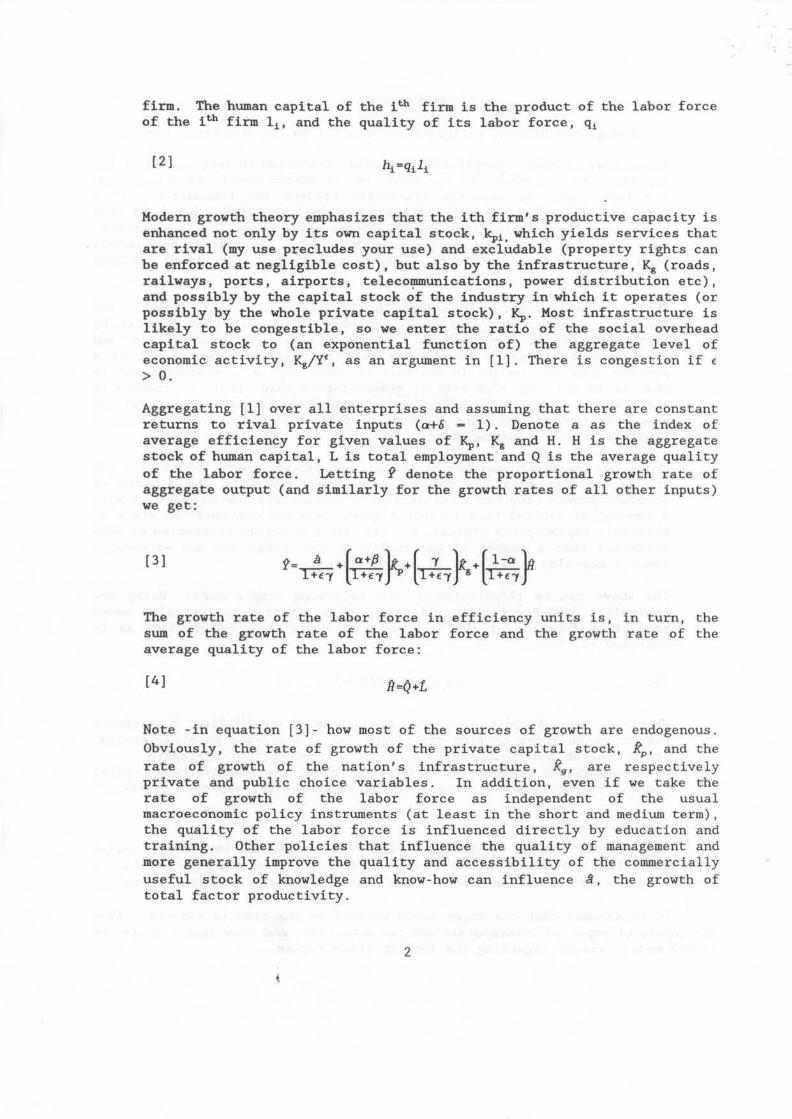
firm. The human capital of the ith firm is the product of the labor forcéof the ith firm Iít and the quality of its labor forcé, q±

[ 2 ] h !

Modern growth theory emphasizes that the ith firm's productive capacity isenhanced not only by its own capital stock, kp^ which yields services thatare rival (my use precludes your use) and excludable (property rights canbe enforced at negligible cost) , but also by the inf ras truc tur e, Kg (roads,railways, ports, airports, telecommunications, power distribution etc),and possibly by the capital stock of the industry in which it operates (orpossibly by the whole private capital stock), Kp. Most infrastructure islikely to be congestible, so we enter the ratio of the social overheadcapital stock to (an exponential function of) the aggregate level ofeconomic activity, Kg/Y

e, as an argument in [1] . There is congestión if e> 0.

Aggregating [1] over all enterprises and assuming that there are constantreturns to rival private inputs (a+6 = 1) . Denote a as the índex ofaverage efficiency for given valúes of Kp, Kg and H. H is the aggregatestock of human capital, L is total employment and Q is the average qualityof the labor forcé. Letting 9 denote the proportional growth rate ofaggregate output (and similarly for the growth rates of all other inputs)we get:

[3]

The growth rate of the labor forcé in efficiency units is , in turn, thesum of the growth rate of the labor forcé and the growth rate of theaverage quality of the labor forcé:

Note -in equation [3]- how most of the sources of growth are endogenous .

Obviously, the rate of growth of the private capital stock, £p, and the

rate of growth of the nation's infrastructure, Kg, are respectivelyprivate and public choice variables. In addition, even if we take therate of growth of the labor forcé as independent of the usualmacroeconomic policy instrumenta (at least in the short and médium term) ,the quality of the labor forcé is influenced directly by education andtraining. Other policies that influence the quality of management andmore generally improve the quality and accessibility of the commercially

useful stock of knowledge and know-how can influence á , the growth oftotal factor productivity.

The practical policy implications, of the above, are that there should bean increase in expenditure (both public and prívate) on: (i)infrastructure, Kg, and its composition should be directed at reducingcongestión,e , (ii) on health and education and targeted anti-povertyprograms to increase H, (iii) structural reforms in general to increasetotal factor productivity, a.

Although not dírectly captured in the above simple model, recent empiricalwork, invoking modern growth theory, suggests that more open economieshave higher rates of growth. By using their resources more efficientlythey achieve a higher level of saving, investment and ultimately growth.Further countries that are open to trade produce with more up-to-datetechnology, and invest more in quality improvement and research anddevelopment. After controlling for factor accumulation, studies alsosuggest that financial deregulation, from initially distorted posítion,also has a positive effect on growth. Although in this case care has to betaken in the speed and the sequence of reform. The relation between fiscalpolicy and growth is a complex one, and country specific, however, it hasa negative effect on growth particularly when funds are wasted onworthless projects, there are bloated bureaucracies, and when taxes andregulations dístort savings and investment decisions. Finally empiricalevidence suggests that the lower the regulatory distortion and higher theexpenditure on education and health the greater the rate of growth.

In the DR, the growth record of the last decade has been disappointing.Real per capita GDP is essentially where it was fifteen years ago.Population is still growing very rapidly (around 2.3 per cent per annum),putting considerable strain on the nation's environmental, health,educational and housing resources. Human capital formation is not takingplace in the quantity and quality necessary for a human resources drivenimprovement in the economic growth record. Fiscal expenditures onEducation declined over the 1980's as a share of total government spendingand of GNP. By the late 1980s the ratio of public expenditure on educationto GDP represented less than half the average for Latin America. Prívatespending on education increased but not by enough to offset the decline inpublic resources, especially among the poorest groups. Higher educationcontinúes to absorb a disproportionally large share of the scarceeducational resources. Support from the Multilaterals for vocationaltraining, including on-the-job-training, in collaboration and partnershipwith prívate firms, industrial or trade associations and with thegovernment, might be a productive use of resources.

The relatively high life expectancy at birth (69 years for women and 65years for men) belie the fact that the health status of much of thepopulation is poor and may well be deteriorating. Apart from the humansuffering this entails, it also constitutes a direct drag on the nation'sproductive potential. Some of the major public health problems (such aswater-borne and -related diseases) directly reflect the history ofinadequate infrastructure investment in sanitation and potable water.

Physical capital formation rates have declined, hovering around 15% of GDP

for gross prívate capital formation and varying for the public sector fromover 11X of GDP in 1989 to just over 8% of GDP in 1992. The productivity(or ICOR) of part of past investment is certain to have been sunk incapital goods appropriate to the oíd, distorted relative price structure.It should no longer be expected to be viable now that prices are closer tothe true opportunity costs.

The recent reforms can be viewed, in terms of equation [3], as an attemptto raise á, the growth rate of total factor productivity. While they arelikely to do so in the médium to long run, if they are credible and areactually adhered to. they are certain to cause dislocation and increasedtransitory unemployment in the short run, as factors of production areredirected towards their proper uses. Beyond the gains from reform, anysustained increase in the growth rate will require an increase in the rateof accumulation, broadly defined to include both prívate and public fixeddomestic capital formation as well as human capital accumulation throughimprovements in public health, education and training. The vast world-wide stock of productive knowledge cannot be transplanted to the DominicanRepublic and turned into local commercially useful knowledge and know-howwithout significant prívate and also public investment.

•