Domain Theory In Logical Form

Samson Abramsky

Department of Computing

Imperial College of Science and Technology

180 Queen’s Gate

London SW7 2BZ

England

Published in Annals of Pure and Applied Logic 51 (1991) 1–77

September 2, 1988

Abstract

The mathematical framework of Stone duality is used to synthesize a numberof hitherto separate developments in Theoretical Computer Science:

• Domain Theory, the mathematical theory of computation introduced byScott as a foundation for denotational semantics.

• The theory of concurrency and systems behaviour developed by Milner,Hennessy et al. based on operational semantics.

• Logics of programs.

Stone duality provides a junction between semantics (spaces of points = denota-tions of computational processes) and logics (lattices of properties of processes).Moreover, the underlying logic is geometric, which can be computationally in-terpreted as the logic of observable properties—i.e. properties which can bedetermined to hold of a process on the basis of a finite amount of informationabout its execution.

These ideas lead to the following programme:

1. A metalanguage is introduced, comprising

• types = universes of discourse for various computational situations.

• terms = programs = syntactic intensions for models or points.

2. A standard denotational interpretation of the metalanguage is given, as-signing domains to types and domain elements to terms.

3. The metalanguage is also given a logical interpretation, in which typesare interpreted as propositional theories and terms are interpreted via aprogram logic, which axiomatizes the properties they satisfy.

4. The two interpretations are related by showing that they are Stone dualsof each other. Hence, semantics and logic are guaranteed to be in harmonywith each other, and in fact each determines the other up to isomorphism.

5. This opens the way to a whole range of applications. Given a denotationaldescription of a computational situation in our meta-language, we canturn the handle to obtain a logic for that situation.

Organization

Chapter 1 is an introduction and overview. Chapter 2 gives some background ondomains and locales. Chapters 3 and 4 are concerned with 1–4 above. Finally,Chapter 5 discusses directions for further research.

Contents

1 Introduction 21.1 Background . . . . . . . . . . . . . . . . . . . . . . . . . . . . . . 21.2 Overview: Stone Duality . . . . . . . . . . . . . . . . . . . . . . . 4

2 Background: Domains and Locales 72.1 Notation . . . . . . . . . . . . . . . . . . . . . . . . . . . . . . . . 72.2 Domains . . . . . . . . . . . . . . . . . . . . . . . . . . . . . . . . 82.3 Locales . . . . . . . . . . . . . . . . . . . . . . . . . . . . . . . . 142.4 Domains and Locales . . . . . . . . . . . . . . . . . . . . . . . . . 18

3 Domain Pre-Locales 213.1 Introduction . . . . . . . . . . . . . . . . . . . . . . . . . . . . . . 213.2 A Category of Pre-Locales . . . . . . . . . . . . . . . . . . . . . . 213.3 A Cpo of Pre-Locales . . . . . . . . . . . . . . . . . . . . . . . . 263.4 Constructions . . . . . . . . . . . . . . . . . . . . . . . . . . . . . 293.5 Logical Semantics of Types . . . . . . . . . . . . . . . . . . . . . 43

4 Domain Logics 484.1 Introduction . . . . . . . . . . . . . . . . . . . . . . . . . . . . . . 484.2 Domains as Propositional Theories . . . . . . . . . . . . . . . . . 514.3 Programs as Elements: Endogenous Logic . . . . . . . . . . . . . 604.4 Programs as Morphisms: Exogenous Logic . . . . . . . . . . . . . 714.5 Applications: The Logic of a Domain Equation . . . . . . . . . . 77

5 Conclusion 785.1 Further Directions . . . . . . . . . . . . . . . . . . . . . . . . . . 785.2 Related Work . . . . . . . . . . . . . . . . . . . . . . . . . . . . . 805.3 Acknowledgements . . . . . . . . . . . . . . . . . . . . . . . . . . 80

References 81

1

Chapter 1

Introduction

Our aim is to synthesize a number of hitherto separate developments in Theo-retical Computer Science:

• Domain Theory, the mathematical theory of computation introduced byScott as a foundation for denotational semantics.

• The theory of concurrency and systems behaviour developed by Milner,Hennessy et al. based on operational semantics.

• Logics of programs.

The key to our synthesis is the mathematical theory of Stone duality, whichprovides a junction between semantics (spaces of points = denotations of com-putational processes) and logics (lattices of properties of processes). Moreover,the underlying logic is geometric, which can be computationally interpreted asthe logic of observable properties—i.e. properties which can be determined tohold of a process on the basis of a finite amount of information about its exe-cution. As a worked example, we show how Domain Theory can be construedas a logic of observable properties; applications to the study of programminglanguages will be presented elsewhere [Abr88, Abr87a].

1.1 Background

Domain Theory has been extensively studied since it was introduced by Scott[Sco70], both as regards the basic mathematical theory [Plo81], and the applica-tions, particularly in denotational semantics [MS76, Sto77, Gor79, Sch86], andmore recently in static program analysis [Myc81, Nie84, AH87]. In the courseof this development, a number of new perspectives have emerged.

Syntax vs. Semantics

Domain theory was originally presented as a model theory for computation, andthis aspect was emphasised in [Sco70, Sco80]. However, the effective characterof domain constructions was immediately evident, and made fully explicit in[EC76, Sco76, Smy77, Kan79]. Moreover, in recent presentations of domains

2

via neighbourhood systems and information systems [Sco81, Sco82], Scott hasshown how the theory can be based on elementary, and finitary, set-theoreticrepresentations, which in the case of information systems are deliberately sug-gestive of proof theory.

A further step towards explicitly syntactic presentations of domain theorywas taken by Martin-Lof, in his Domain Interpretation of Intuitionistic TypeTheory [ML83]. His formulation also traces a line of descent from Kreisel’sdefinition of the continuous functionals [Kre59], via [ML70, Ers72].

The general tendency of these developments is to suggest that domains mayas well be viewed in terms of theories as of models. Our work should not onlyconfirm this suggestion, but also show how it may be put to use.

Points vs. Properties

An important recent development in mathematics has been the rise of localetheory, or “topology without points” [Joh82], in which the open-set latticesrather than the spaces of points become the primary objects of study. Thatthese mathematical developments have direct bearing on Computer Science wasemphasised by Smyth in [Smy83b]. If we think of the open sets as propertiesor propositions, we can think of spaces as logical theories; continuous maps acton these theories under inverse image as predicate transformers in the sense ofDijkstra [Dij76], or modal operators as studied in dynamic logic [Pra81, Har79].

There is also an important theme in Computer Science which emerges asconfluent with these mathematical developments; namely, the use of notions ofobservation and experiment as a basis for the behavioural semantics of systems.This plays a major role in the work of Milner, Hennessy et al. on concurrentsystems [Mil80, HM85, Win80], and also in the theory of higher-order functionallanguages, e.g. [Plo77, Mil77, BC85, BCL85]. The leading idea here is to takesome notion of observable event or experiment as an “information quantum”,and to construct the meaning of a system out of its information quanta. Thiscorresponds to the leading idea of locale theory, that “points” are nothing butconstructions out of properties. By exploiting this correspondence, we may hopeto obtain a rapprochement between domain theory and denotational semantics,on the one hand, and operationally formulated notions such as observationequivalence [HM85] on the other.

Denotational vs. Axiomatic

Another area in programming language theory which has received intensivedevelopment over the past 15 years has been logics of programs, e.g. Hoarelogic [Hoa69, dB80], dynamic logic [Pra81, Har79], temporal logic [Pnu77], etc.However, to date there has not been a satisfactory integration of this workwith domain theory. For example, dynamic logic deals with sets and relations,which from the perspective of domain theory corresponds only to an extremelynaive and restricted fragment of programming language semantics. One wouldlike to see a dynamic logic of domains and continuous functions, which wouldencompass higher-order functions, quasi-infinite (or “lazy”) data structures,

3

self-application, non-determinism, and all the other computational phenomenafor which domain theory provides a mathematical foundation.

The key mathematical idea which forms the basis of our attempt to drawall these diverse strands together is Stone Duality, which we now briefly review;a fuller discussion will be found in Chapter 2.

1.2 Overview: Stone Duality

The classic Stone Representation Theorem for Boolean algebras [Sto36] is aimedat solving the following problem:

show that every (abstract) Boolean algebra can be represented as afield of sets, in which the operations of meet, join and complementare represented by intersection, union and set complement.

Stone’s solution to the problem begins with observation that for any topo-logical space X, the lattice Clop X of clopen subsets of X forms a field of sets.His radical step was to construct, from any Boolean algebra B, a topologicalspace Spec B. To understand the construction, think of B as (the Lindenbaumalgebra of) a classical propositional theory. The elements of B are thus to bethought of as (equivalence classes of) formulae, and the operations as logicalconjunction, disjunction and negation. Now a model of B is an assignment of“truth-values” 0 or 1 to elements of B, in a manner consistent with the logicalstructure; e.g. so that ¬b is assigned 1 if and only if b is assigned 0. In short,a model is a Boolean algebra homomorphism f : B → 2, where 2 = 0, 1 isthe two-element lattice. Identifying such an f with f−1(1) ⊆ B, which as iswell-known is an ultrafilter over B (see e.g. [Joh82]), we can take Spec B as theset of ultrafilters over B, with the topology generated by

Ua ≡ x ∈ Spec B : a ∈ x (a ∈ B).

The spaces arising as Spec B for Boolean algebras B in this way were char-acterised by Stone as the totally disconnected compact Hausdorff spaces (sub-sequently named Stone spaces in his honour). Moreover, we have the isomor-phisms

B ∼= Clop Spec B b 7→ x ∈ Spec B : b ∈ x (1.1)

S ∼= Spec Clop S s 7→ U ∈ Clop S : s ∈ U. (1.2)

The first of these isomorphisms solves the representation problem, and com-prises Stone’s Theorem in its classical form. But we can go further; thesecorrespondences also extend (contravariantly) to morphisms:

Sf−→ T

Clop Sf−1

←− Clop T

Ah?

←− BSpec A

h−→ Spec B

whereh : x 7→ b ∈ B : h?b ∈ x.

4

In modern terminology, this yields a duality (= contravariant equivalence ofcategories):

Stone ' Boolop.

This is the prototype for a whole family of “Stone-type duality theorems”, andleads to locale theory, as “pointless topology” or junior-grade (propositional)topos theory. (An excellent reference for these topics is [Joh82]).

But what has all this to do with Computer Science? Two interpretationsof Stone duality can be found in the existing literature from mathematics andlogic:

• The topological view: Points vs. Open sets.

• The logical view: Models vs. Formulas.

We wish to add a third interpretation:

• The Computer Science view: (Denotations of) computational processesvs. (extensions of) specifications.

The importance of Stone duality for Computer Science is that it provides theright framework for understanding the relationship between denotational seman-tics and program logic. The fundamental logical relationship of program devel-opment is

P |= φ

to be read “P satisfies φ”, where P is a program (a syntactic description of acomputational process), and φ is a formula (a syntactic description of a propertyof computations). Thus P is the “how” and φ the “what” in the dichotomystandardly used to explain the distinction between programs and specifications.We can easily describe the main formal activities of the program developmentprocess in terms of this relation:

• Program specification is the task of defining (a list of) properties φ to besatisfied by the program.

• Program synthesis is the task of finding P given (a list of) φ.

• Program verification is the task of proving that P |= φ.

The two sides of Stone duality—the spatial and the logical or localic—yieldalternative but equivalent perspectives on this fundamental relationship:

• The spatial side of the duality, where points are taken as primary, prop-erties are constructed as (open) sets of points, and the fundamental rela-tionship is interpreted as s ∈ U (s a point, U a property), corresponds todenotational semantics, where the data domains (i.e. the types) of a pro-gramming language are interpreted as spaces of points, and programs aregiven denotations as points in these spaces; this denotational perspectiveyields a topological interpretation of program logic.

5

• The logical or localic side of the duality, where properties, as elementsof an abstract (logical) lattice, are taken as primary, and points are con-structed as sets (prime filters) of properties, with the fundamental rela-tionship interpreted as a ∈ x (a a property, x a point), corresponds toprogram logic, and yields a logical interpretation of denotational seman-tics. The idea is that the structure of the open-set lattices and primefilters are presented syntactically, via axioms and inference rules, as aformal system.

We extract the following concrete research programme from these general per-spectives on Stone duality:

1. A metalanguage is introduced, comprising

• types = data domains = universes of discourse for various computa-tional situations.

• terms = programs = syntactic intensions for models or points.

2. A standard denotational interpretation of the metalanguage, assigningdomains to types and domain elements to terms, can be given using thespatial side of Stone duality.

3. The metalanguage is also given a logical interpretation, in which the lo-calic side of the duality is presented as a formal system with axioms andinference rules. Each type is interpreted as a propositional theory; andterms are interpreted by axiomatising the satisfaction relation P |= φ.This gives a program logic.

4. The denotational semantics from 2 and the program logic from 3 are re-lated by showing that they are Stone duals of each other—a strengthenedform of the logician’s “Soundness and Completeness”. As a consequenceof this, semantics and logic are guaranteed to be in harmony with eachother, and in fact each determines the other up to isomorphism.

5. The framework developed in 1–4 is very general. The metalanguage canbe used to describe a wide variety of computational situations, followingthe ideas of “classical” denotational semantics. Given such a description,we can turn the handle to obtain a logic for that situation. This offers twoexciting prospects: of replacing ad hoc ingenuity in the design of programlogics to match a given semantics by the routine application of systematicgeneral theory; and of bringing hitherto divergent fields of programminglanguage theory (e.g. λ-calculus and concurrency) within the scope of asingle unified framework.

The main objective of this paper is to elaborate the programme outlined in 1–4 above (applications as in 5 will be presented elsewhere [Abr88, Abr87a]).Chapter 2 is devoted to filling in some background on domains and locales. ThenChapters 3 and 4 present our results. Finally, Chapter 5 discusses directionsfor further research.

6

Chapter 2

Background: Domains andLocales

The purpose of this Chapter is to summarise what we assume, to fix notation,and to review some basic definitions and results.

2.1 Notation

Most of the notation from elementary set theory and logic which we will useis standard and should cause no problems to the reader. We shall use ≡ fordefinitional equality; thus M ≡ N means “the expression M is by definitionequal to N” (or just: “is defined to be N”). We shall use ω and N to denote thenatural numbers 0, 1, . . . (thought of sometimes as an ordinal, and sometimesas just a set). Given a set X, we write ℘X for the powerset of X, ℘fX forthe set of finite subsets of X, and ℘fneX for the finite non-empty subsets. Wewrite X ⊆f Y (X ⊆fne Y ) for the assertion that X is a finite (finite non-empty)subset of Y .

We write substitution of N for x in M , where M , N are expressions and xis a variable, as M [N/x]. We shall assume the usual notions of free and boundvariables, as expounded e.g. in [Bar84]. We shall always take expressions mod-ulo α-conversion, and treat substitution as a total operation in which variablecapture is avoided by suitable renaming of bound variables.

Our notations for semantics will follow those standardly used in denotationalsemantics. One operation we will frequently need is updating of environments.Let Env = Var → V, where Var is a set of variables, and V some value space.Then for ρ ∈ Env, x ∈ Var, v ∈ V, the expression ρ[x 7→ v] denotes theenvironment defined by

(ρ[x 7→ v])y =

v, x = y

ρy, otherwise.

Next, we recall some notions concerning posets (partially ordered sets).

7

Given a poset P and X ⊆ P , we write

↓(X) = y ∈ P : ∃x ∈ X. y ≤ x

↑(X) = y ∈ P : ∃x ∈ X.x ≤ y

Con(X) = y ∈ P : ∃x, z ∈ X.x ≤ y ≤ z

UB(X) = y ∈ P : ∀x ∈ X.x ≤ y

MUB(X) = y ∈ UB(X) : ∀z ∈ UB(X). z ≤ y ⇒ y ≤ z

We write ↓(x), ↑(x) for ↓(x), ↑(x). A set X is left-closed (or lower-closed)if X = ↓(X), right-closed (or upper-closed) if X = ↑(X), and convex-closed ifX = Con(X). UB(X) is the set of upper bounds of X, and MUB(X) the minimalupper bounds. When it is important to emphasise P we write ↓P (X), ↑P (X)etc. We also have the lower, upper and Egli-Milner preorders (reflexive andtransitive relations) on subsets of P :

X vl Y ≡ ∀x ∈ X. ∃y ∈ Y. x ≤ y

X vu Y ≡ ∀y ∈ Y.∃x ∈ X.x ≤ y

X vEM Y ≡ X vl Y &X vu Y

We write 2 for the two-element lattice 0, 1 with 0 < 1, and O for Sierpinskispace, which has the same carrier as 2, and topology ∅, 1, 0, 1. As weshall see in the section on domains and locales, 2 and O are really two faces of thesame structure (a “schizophrenic object” in the terminology of [Joh82, Chapter6]), since O arises from the Scott topology on 2, and 2 from the specialisationorder on O. For other basic notions of the theory of partial orders and lattices,we refer to [GHK+80, Joh82].

Finally, we shall assume a modicum of familiarity with elementary cate-gory theory and general topology; suitable references are [ML71] and [Dug66]respectively.

2.2 Domains

We shall assume some familiarity with [Plo81], and use it as our main referencefor Domain theory. We shall also refer to [Gun85, Gun87].

For the reader’s convenience, we briefly review some basic definitions. Let(P,v) be a poset. A subset X ⊆ P is directed if every finite subset of X hasan upper bound in X. (Thus a directed subset is non-empty). A directed-complete partial order (dcpo) is a poset in which every directed subset X has aleast upper bound (written

⊔X). A morphism of dcpo’s is a map f : D → E

satisfyingf(

⊔X) =

⊔f(x) : x ∈ X

for all directed X ⊆ D. Let D be a dcpo. The Scott topology on D, σ(D), isgiven by all subsets U ⊆ D satisfying

8

• U = ↑(U)

•⊔S ∈ U , S directed implies S ∩ U 6= ∅.

Fact 2.2.1 A function f : D → E is a morphism if and only if it is continuouswith respect to the Scott topology.

In the light of this fact, morphisms are referred to as continuous maps.Let (D,v) be a dcpo. An element b ∈ D is finite if, whenever S ⊆ D is

directed and b v⊔S, b v d for some d ∈ S. We write K(D) for the sub-poset

of finite elements of D. A subset B ⊆ D is a basis for D if for every d ∈ D,S = B ∩ ↓(d) is directed, and d =

⊔S. A dcpo is algebraic if K(D) is a basis,

and ω-algebraic if K(D) is also countable. We shall refer to ω-algebraic dcpo’sD with least elements (written ⊥D) as (algebraic) domains. If D is algebraic,the Scott topology has a particularly simple form, namely all sets of the form⋃

i∈I

↑(bi) (bi ∈ K(D), i ∈ I).

Moreover, the compact-open subsets are those of this form with I finite.By a category of domains we shall mean a sub-category of DCPO, the

category of dcpo’s with least elements and continuous functions1. DCPO⊥ isthe sub-category of strict functions, i.e. those satisfying f(⊥) = ⊥.

The properties of DCPO which make it a suitable mathematical universefor denotational semantics—a “tool for making meanings” in Plotkin’s phrase—are:

1. It admits recursive definitions, both of elements of domains, and of do-mains themselves.

2. It supports a rich type structure.

The mathematical content of (1) is given by the least fixed point theorem forcontinuous functions on dcpo’s ([Plo81, Chapter 1 Theorem 1]), and the ini-tial fixed point theorem for continuous functors on DCPO ([Plo81, Chapter5 Theorem 1]). As for (2), the type constructions available over DCPO areextensively surveyed in [Plo81, Chapters 2 and 3]. In order to fix notation, weshall catalogue the constructions of which mention will be made in this paper,with references to the definitions in [Plo81]:

1Plotkin uses a slightly different category CPO in [Plo81]. The difference is marginal, andfor the ω-algebraic case we are mainly concerned with the two notions in fact coincide.

9

A×B product Ch. 2 p. 2

(A→ B) function space Ch. 2 p. 9

A⊕B coalesced sum Ch. 3 p. 6

(A)⊥ lifting Ch. 3 p. 9

(A→⊥ B) strict function space Ch. 1 p. 13

Pl(A) lower (Hoare) powerdomain Ch. 8 p. 14

Pu(A) upper (Smyth) powerdomain Ch. 8 p. 45

P(A) convex (Plotkin) powerdomain Ch. 8 p. 28

(Note that separated sum A+B can be defined by: A+B ≡ (A)⊥⊕(B)⊥.) Mostof these constructions have simple concrete descriptions as operations on dcpo’s.Thus A×B is Cartesian product, ordered componentwise; A→ B is the set ofcontinuous maps, ordered pointwise; A⊕ B is the disjoint union, with bottomelements identified; (A)⊥ is A with a new bottom element adjoined; A →⊥ Bis the set of strict continuous maps, ordered pointwise. The description of thepowerdomains makes some use of topological notions. The Smyth powerdomainis given as all non-empty Scott-compact upper-closed subsets, ordered by su-perset; the Hoare powerdomain as all non-empty Scott-closed subsets, orderedby subset inclusion; the Plotkin powerdomain as all non-empty Scott-compactsubsets S satisfying

S = ↑(S) ∩ S

(where S is the Scott-closure of S), with the Egli-Milner ordering2.In this paper, we shall be concerned with sub-categories of ωALG, the

category of algebraic domains and continuous maps. In particular, we shall beconcerned with the following full sub-category of ωALG:

• The category SFP of strongly algebraic domains [Plo76, Plo81, Gun85,Gun87].

The name is an acronym for “Sequences of Finite Posets”, which arises fromone of the main descriptions of SFP domains, as bilimits (i.e. direct limits ofembeddings, or, equivalently by the “limit-colimit coincidence” [SP82], inverselimits of projections) of sequences of finite posets. The other main descriptionof SFP is “intrinsic”, i.e. expressed in terms of conditions on the poset of finiteelements.

Definition 2.2.2 Let D be an algebraic domain. We say that D is:

• coherent algebraic if K(D) satisfies “property M” [Gun85, Gun87]: forevery finite u ⊆ K(D), MUB(u) is finite, and moreover complete in thesense that

∀x ∈ UB(u).∃y ∈ MUB(u). y v x.2These descriptions are strictly speaking only valid for algebraic domains, but this will be

the only case considered in this paper.

10

• SFP if it is coherent algebraic, and moreover for every finite u ⊆ K(D),U?(u) is finite, where

U?(u) =⋃

k∈ω Uk(u)

U0(u) = u

Uk+1(u) =⋃MUB(v) : v ⊆ Uk(u)

The justification for studying this category comes from the fact that SFP isclosed under all the type constructions listed above. In particular, it is cartesianclosed; indeed, SFP is the largest cartesian closed full sub-category of ωALG[Smy83a]. Moreover, it admits initial solutions of domain equations built fromthese constructions. Almost all the domains needed in denotational semanticsto date can be defined from these constructions by composition and recursion(some exceptions of three different kinds: [Abr83], [Ole85], [Plo82]).

Now algebraic domains are freely constructed from their bases, i.e.

D ∼= Idl(K(D))

where Idl(P ), for any poset P , is the ideal completion formed by taking alldirected, left-closed subsets of P , ordered by inclusion [Plo81, Chapter 6 p.5]. Thus we can in fact completely describe such categories as SFP in anelementary fashion in terms of the bases; various ways of doing this for a certainsub-category of SFP (the “Scott domains”) are presented in [Sco81, Sco82].

An important part of this programme is to describe the type constructionslisted above in terms of their effect on the bases. We shall fix some concretedefinitions of the constructions for use in later chapters.

• K(A×B) = K(A)×K(B); the ordering is component-wise.

• K(A⊕B) = K(A)⊕K(B), i.e.

⊥ ∪ (0 × (K(A) \ ⊥A)) ∪ (1 × (K(B) \ ⊥B))

with the ordering defined by

x v y ≡ x = ⊥or x = (0, a) & y = (0, b) & a vA b

or x = (1, c) & y = (1, d) & c vB d.

• K((A)⊥) = ⊥ ∪ (0 × K(A)), with the ordering defined by

x v y ≡ x = ⊥or x = (0, a) & y = (0, b) & a vA b.

• K(Pl(A)) = ↓K(A)(X) : X ∈ ℘fne(K(A)), with the subset ordering.

• K(Pu(A)) = ↑K(A)(X) : X ∈ ℘fne(K(A)), with the superset ordering.

11

• K(P(A)) = ConK(A)(X) : X ∈ ℘fne(K(A)), with the Egli-Milner order-ing (which is a partial order on the convex-closed sets).

All these definitions are valid for any algebraic domain. Since ωALG is notcartesian closed, we shall describe the function space construction for its largestcartesian closed sub-category, SFP. Our description will follow [Gun85, Gun87].

Definition 2.2.3 (i) ([Plo81, Chapter 6 p. 1]). Let A, B be algebraic domains.For a ∈ K(A), b ∈ K(B),

(ab) : A→ B

is the one-step function defined by

(ab)d =

b if a v d

⊥ otherwise

(ii) ([Gun85, Gun87]). u ⊆fne K(A)×K(B) is joinable (notation: 4(u)) iff forall a ∈ K(A), (a′, b′) ∈ u : a′ v a has a maximum in K(A)×K(B).

(iii) Given 4(u), define due : A→ B by

due(d) = maxb : ∃a. (a, b) ∈ u& a v d.

Note that Plotkin writes (a⇒ b) for (ab).

Proposition 2.2.4 ([Gun87, Theorem 13]). Let A, B be SFP domains, andu ⊆fne K(A)×K(B) such that 4(u).(i) due is a continuous function, and a finite element of (A→ B). In fact, wehave

due =⊔(ab) : (a, b) ∈ u.

(ii) due v dve ⇐⇒ ∀(a, b) ∈ u.∃(a′, b′) ∈ v. a′ v a& b v b′.(iii) (A→ B) is algebraic, and in fact an SFP domain, with basis given by

K(A→ B) = due : u ⊆fne K(A)×K(B) & 4 (u).

The definition of 4(u) has the unwelcome feature of a universal quantifica-tion over K(A). The following Proposition (which is new) gives an alternative,more “local” (and hence more easily effectivized) description.

Notation. Given a set X of ordered pairs, we write (X)1 ((X)2) for theset of first (second) components of elements of X.

Proposition 2.2.5 Let A, B be coherent algebraic domains, u ⊆fne K(A) ×K(B). Then 4(u) iff

∀v ⊆ u. ∃w ⊆ u. (w)1 = MUB((v)1) & [∀b ∈ (v)2, b′ ∈ (w)2. b v b′]. (2.1)

Proof. (⇒). Consider v ⊆ u. For each m ∈ MUB((v)1), 4(u) implies that

zm = (a′, b′) ∈ u : a′ v m

12

has a maximum element (am, bm). Let w = (am, bm) : m ∈ MUB((v)1). Sincev ⊆ zm, am ∈ UB((v)1) for each m. Also, am v m; hence by minimality of m,am = m, and (w)1 = MUB((v)1). Finally, v ⊆ zm implies bm ∈ UB((v)2) foreach m.

(⇐). Given a ∈ K(A), consider the set

v = (a′, b′) ∈ u : a′ v a.

For some w ⊆ u, (w)1 = MUB((v)1). Since a ∈ UB((v)1), for some (a′, b′) ∈ w,a′ v a. Hence (a′, b′) ∈ v. Moreover, b′ ∈ UB((v)2). Thus (a′, b′) is the requiredmaximum for v.

We conclude this section by reviewing some notions on embeddings, whichplay an important role in the standard category-theoretic account of the solutionof domain equations [SP82]. Recall that an embedding-projection pair betweendomains D, E is a pair of continuous functions e : D → E, p : E → D satisfying

p e = idD, e p v idE .

Each of these functions uniquely determines the other, since e is left adjoint to p.We write eR for the projection determined by e. It is standard that embeddingsare strict, order-reflecting (i.e. e(x) v e(y)⇒ x v y), and carry finite elementsto finite elements. Moreover, since they are left adjoints they preserve all joins.The following Proposition (which I have not found in the literature) is simplebut useful; it says that the formation of bases for the various type constructionscommutes with embeddings.

Proposition 2.2.6 Let ei : Ai → Bi (i = 1, 2), e : A → B be embeddings.Then:

(i) (e1 × e2)((a, b)) = (e1(a), e2(b))

(ii) (e1 → e2)(due) = d(e1(a), e2(b)) : (a, b) ∈ ue

(iii) P(e)(Con(x1, . . . , xn)) = Con(e(x1), . . . , e(xn))

(iv) (e1 ⊕ e2)((i, d)) = (i, ei+1(d)) (i = 0, 1)

(v) (e)⊥((0, a)) = (0, e(a))

Proof. We shall verify (ii). Firstly, since embeddings preserve joins, by Propo-sition 2.2.4 it suffices to verify that (e1 → e2)((ab)) = (e1(a)e2(b)). Bydefinition ([SP82]), (e1 → e2)(f) = e2 f eR1 ; while e1 left adjoint to eR1 meansthat

e1(a) v d ⇐⇒ a v eR1 (d).

Now

(e1 → e2)((ab))(d) =

e2(b), a v eR1 (d)

⊥ otherwise

=

e2(b), e1(a) v d

⊥ otherwise

= (e1(a)e2(b))(d).

13

2.3 Locales

Our reference for locale theory and Stone duality will be [Joh82]. Since localetheory is not yet a staple of Computer Science, we shall briefly review some ofthe basic ideas.

Classically, the study of general topology is based on the category Topof topological spaces and continuous maps. However, in recent years mathe-maticians influenced by categorical and constructive ideas have advocated thatattention be shifted to the open-set lattices as the primary objects of study.Given a space X, we write Ω(X) for the lattice of open subsets of X ordered byinclusion. Since Ω(X) is closed under arbitrary unions and finite intersections,it is a complete lattice satisfying the infinite distributive law

a ∧∨S =

∨a ∧ s : s ∈ S.

(By the Adjoint Functor Theorem, in any complete lattice this law is equivalentto the existence of a right adjoint to conjunction, i.e. to the fact that implica-tion can be defined in a canonical way.) Such a lattice is a complete Heytingalgebra, i.e. the Lindenbaum algebra of an intuitionistic theory. The continu-ous functions between topological spaces preserve unions and intersections, andhence all joins and finite meets of open sets, under inverse image; thus we geta functor

Ω : Top→ Loc

where Loc, the category of locales, is the opposite of Frm, the category offrames, which has complete Heyting algebras as objects, and maps preservingall joins and finite meets as morphisms. Note that Frm is a concrete categoryof structured sets and structure-preserving maps, and consequently convenientto deal with (for example, it is monadic over Set). Thus we study Loc viaFrm; but it is Loc which is the proposed alternative or replacement for Top,and hence the ultimate object of study.

Notation. Given a morphism f : A → B in Loc, we write f? for thecorresponding morphism B → A in Frm.

Now we can define a functor

Pt : Loc→ Top

as follows (for motivation, see our discussion of Stone’s original construction inChapter 1): Pt(A) is the set of all frame morphisms f : A→ 2, where 2 is thetwo-point lattice. Any such f can be identified with the set F = f−1(1), whichsatisfies:

• 1 ∈ F

• a, b ∈ F ⇒ a ∧ b ∈ F

• a ∈ F, a ≤ b ⇒ b ∈ F

•∨

i∈I ai ∈ F ⇒ ∃i ∈ I. ai ∈ F.

Such a subset is called a completely prime filter. Conversely, any completelyprime filter F determines a frame homomorphism χF : A → 2. Thus we can

14

identify Pt(A) with the completely prime filters over A. The topology on Pt(A)is given by the sets Ua (a ∈ A):

Ua ≡ x ∈ Pt(A) : a ∈ x.

Clearly,Pt(A) = U1, Ua ∩ Ub = Ua∧b,

⋃i∈I

Uai = U∨i∈I

ai,

so this is a topology. Pt is extended to morphisms by:

Af?

←− B

Pt(A)Pt(f)−→ Pt(B)

Pt(f)x = b : f?b ∈ x.

We now define, for each X in Top and A in Loc:

ηX : X → Pt(Ω(X)) ηX(x) = U : x ∈ U

εA : Ω(Pt(A))→ A ε?A(a) = x : a ∈ x.

Now we have

Theorem 2.3.1 ([Joh82, II.2.4]). (Ω,Pt, η, ε) : Top Loc defines an ad-junction between Top and Loc; moreover ([Joh82, II.2.7]), this cuts down toan equivalence between the full sub-categories Sob of sober spaces and SLoc ofspatial locales.

The equivalence between Sob and SLoc (and therefore the duality or con-travariant equivalence between Sob and SFrm) may be taken as the mostgeneral purely topological version of Stone duality. For our purposes, somedualities arising as restrictions of this one are of interest.

Definition 2.3.2 A space X is coherent if the compact-open subsets of X(notation: KΩ(X)) form a basis closed under finite intersections, i.e. for whichKΩ(X) is a distributive sub-lattice of Ω(X).

Theorem 2.3.3 (i) ([Joh82, II.2.11]). The forgetful functor from Frm toDLat, the category of distributive lattices, has as left adjoint the functor Idl,which takes a distributive lattice to its ideal completion.(ii) ([Joh82, II.3.4]). Given a distributive lattice A, define Spec(A) as the setof prime filters over A (i.e. sets of the form f−1(1) for lattice homomorphismsf : A→ 2), with topology generated by

Ua ≡ x ∈ Spec(A) : a ∈ x (a ∈ A).

Then Spec(A) ∼= Pt(Idl(A)).(iii) ([Joh82, II.3.3]). The duality of Theorem 2.3.1 cuts down to a duality

CohSp ' CohLoc ' DLatop

where CohSp is the category of coherent T0 spaces, and continuous maps whichpreserve compact-open subsets under inverse image; and CohLocop is the imageof DLat under the functor Idl.

15

The logical significance of the coherent case is that finitary syntax—specificallyfinite dis-junctions—suffices. The original Stone duality theorem discussed inChapter 1 is obtained as the further restriction of this duality to coherent Haus-dorff spaces (which turns out to be another description of the Stone spaces) andBoolean algebras, i.e. complemented distributive lattices. Note that under thecompact Hausdorff condition, all continuous maps satisfy the special propertyin part (iii) of the Theorem.

As a further special case of Stone duality, we note:

Theorem 2.3.4 (i) The forgetful functor from distributive lattices to the cat-egory MSL of meet-semilattices has a left adjoint L, where L(A) = ↓(X) :X ∈ ℘f(A), ordered by inclusion. (Notice that this is the same construction asfor the lower powerdomain; this fact is significant, but not in the scope of thispaper.)(ii) For any meet-semilattice A, define Filt(A) as the set of all filters over A,with topology defined exactly as for Spec(A). Then

Filt(A) ∼= Spec(L(A)) ∼= Pt(Idl(L(A))).

(iii) The duality of Theorem 2.3.3 cuts down to a duality

AlgLat 'MSLop

where AlgLat is the full sub-category of CohSp of algebraic lattices with theScott topology.

An extensive treatment of locale theory and Stone-type dualities can befound in [Joh82]. Our purpose in the remainder of this section is to give someconceptual perspectives on the theory.

Firstly, a logical perspective. As already mentioned, locales are the Lin-denbaum algebras of intuitionistic theories, more particularly of propositionalgeometric theories, i.e. the logic of finite conjunctions and infinite disjunctions.The morphisms preserve this geometric structure, but are not required to pre-serve the additional “logical” structure of implication and negation (which canbe defined in any complete Heyting algebra). Thus from a logical point of view,locale theory is propositional geometric logic. Moreover, Stone duality also hasa logical interpretation. The points of a space correspond to models in thelogical sense; the theory of a model is the completely prime filter of opens itsatisfies, where the satisfaction relation is just

x |= a ≡ x ∈ a

in terms of spaces, (i.e. with x ∈ X and a ∈ Ω(X)), and

x |= a ≡ a ∈ x

in terms of locales (i.e. with x ∈ Pt(A) and a ∈ A). Spatiality of a classof locales is then a statement of Completeness: every consistent theory has amodel.

16

Secondly, a computational perspective. If we view the points of a space as thedenotations of computational processes (programs, systems), then the elementsof the corresponding locale can be seen as properties of computational processes.More than this, these properties can in turn be thought of as computationallymeaningful; we propose that they be interpreted as observable properties. In-tuitively, we say that a property is observable if we can tell whether or not itholds of a process on the basis of only a finite amount of information about thatprocess3. Note that this is really semi-observability, since if the property is notsatisfied, we do not expect that this is finitely observable. This intuition ofobservability motivates the asymmetry between conjunction and disjunction ingeometric logic and topology. Infinite disjunctions of observable properties arestill observable—to see that

∨i∈I ai holds of a process, we need only observe

that one of the ai holds—while infinite conjunctions clearly do not preservefinite observability in general. More precisely, consider Sierpinski space O. Wecan regard this space as representing the possible outcomes of an experiment todetermine whether a property is satisfied; the topology is motivated by semi-observability, so an observable property on a space X should be a continuousfunction to O. In fact, we have

Ω(X) ∼= (X → O)

where (X → O) is the continuous function space, ordered pointwise (thinkingof O as 2). Now for infinite I, I-ary disjunction, viewed as a function∨

: OI → O

is continuous, while I-ary conjunction is not. Similarly, implication and nega-tion, taken as functions

⇒: O2 → O, ¬ : O→ O

are not continuous. Thus from this perspective,

geometric logic = observational logic.

These ideas follow those proposed by Smyth in his pioneering paper [Smy83b],but with some differences. In [Smy83b], Smyth interprets “open set” as semi-decidable property; this represents an ultimate commitment to interpret ourmathematics in some effective universe. My preference is to do TheoreticalComputer Science in as ontologically or foundationally neutral a manner aspossible. The distinction between semi-observability and semi-decidability isanalogous to the distinction between the computational motivation for the ba-sic axioms of domain theory in terms of “physical feasibility” given in [Plo81,Chapter 1], without any appeal to notions of recursion theory; and a commit-ment to only considering computable elements and morphisms of effectively

3This is really only one facet of observability. Another is extensionality, i.e. that we regarda process as a black box with some specified interface to its environment, and only takewhat is observable via this interface into account in determining the meaning of the process.Extensionality in this sense is obviously relative to our choice of interface; it is orthogonal tothe notion being discussed in the main text.

17

given domains, as advocated in [Kan79]. It should also be said that the link be-tween observables and open sets in domain theory was clearly (though briefly!)stated in [Plo81, Chapter 8 p. 16], and used there to motivate the definition ofthe Plotkin powerdomain.

A final perpective is algebraic. The category Frm is algebraic over Set([Joh82, II.1.2]); thus working with locales, we can view topology as a species of(infinitary) algebra. In particular, constructions of universal objects of variouskinds by “generators and relations” are possible. Two highly relevant examplesin the locale theory literature are [Joh85] and [Hyl81]. This provides a link withthe information systems approach to domain theory as in [Sco82, LW84]. Someof our work in Chapters 3 and 4 can be seen as a systematization of these ideasin an explicitly syntactic framework.

2.4 Domains and Locales

We now turn to the connections between domains and locales. We have alreadyseen that domains can be viewed topologically, via the Scott topology.

Given a space X, we define the specialisation order on X by

x ≤spec y ≡ ∀U ∈ Ω(X). x ∈ U ⇒ y ∈ U.

Proposition 2.4.1 ([Plo81, Chapter 1 p. 16]). Let D be a dcpo. The spe-cialisation order on the space (D,σ(D)) coincides with the original ordering onD.

Thus we may regard domains indifferently as posets or as spaces with the Scotttopology.

We now relate domains to coherent spaces.

Theorem 2.4.2 (The 2/3 SFP Theorem) ([Plo81, Chapter 8 p. 41], [Gun85,Theorem 4.19]). An algebraic domain is coherent as a space iff it is “2/3 SFP”in the terminology of (loc. cit.), i.e. satisfies property M as defined in Sec-tion 2.2. By Stone duality for coherent spaces (Theorem 2.3.3), any such do-main D satisfies

D ∼= Spec(KΩ(D)).

This justifies our terminology for such domains as coherent algebraic. ThusSFP is a category of coherent spaces, and we need only consider the lattices ofcompact-open sets on the logical side of the duality.

We conclude with some observations which show how the finite elementsin a coherent algebraic domain play an ambiguous role as both points andproperties. Firstly, we have

D ∼= Idl(K(D))

so the finite elements determine the structure of D on the spatial side. Wecan also recover the finite elements in purely lattice-theoretic terms from A =

18

KΩ(D). Say that a ∈ A is coprime if a ≤∨

i∈I bi, I finite, implies a ≤ bi forsome i ∈ I. Writing cpr(A) for the set of coprimes of A, we have

K(D) = (cpr(A))op, A ∼= L((K(D))op). (2.2)

(The fact that the latter construction produces a distributive lattice even thoughK(D) is not a meet-semilattice follows from the property M axiom for coherentalgebraic domains).

Proposition 2.4.3 ([Gun85, Lemma 4.18]). Suppose X, Y are subsets of aposet P . Then Y is a complete set of upper bounds for X iff:⋂

x∈X

↑(x) =⋃

y∈Y

↑(y). (2.3)

Moreover, if Y is finite and (2.3) holds, then it contains a complete set ofminimal upper bounds for X.

Proof. (⇒). If d ∈⋂

x∈X ↑(x) then d ∈ UB(X), and so for some y ∈ Y , y v d,and d ∈

⋃y∈Y ↑(y). If d w y, y ∈ Y , then d is an upper bound for X, hence

d ∈⋂

x∈X ↑(x).(⇐). Firstly,

⋃y∈Y ↑(y) ⊆

⋂x∈X ↑(x) implies Y ⊆ UB(X), while the con-

verse inclusion implies that Y contains a complete set of upper bounds for X. IfY is finite, it must contain a complete minimal subset, which will be a completeset of minimal upper bounds for X.

The significance of this proposition is that it shows how to turn the MUBaxioms for coherent algebraic and SFP domains into logical axioms about theirlattices of compact-open subsets. It also shows how to translate the descriptionof 4(u) given in Proposition 2.2.5 into an appropriate axiom in our logicaltreatment of function spaces.

Definition 2.4.4 ([Gun85, Theorem 4.19]). We say that a subset X ⊆ A of alattice is quasi-conjunctively closed if for every u ⊆f X, for some v ⊆f X,∧

u =∨v.

X is a quasi-conjunctive closure of Y , X,Y ⊆ A, if Y ⊆ X and X is quasi-conjunctively closed.

The following result gives a purely lattice-theoretic description of those dis-tributive lattices which arise as the compact opens of SFP domains.

Theorem 2.4.5 Let A be a countable distributive lattice. Spec(A) is a coherentalgebraic domain in its Scott topology iff the following conditions are satisfied:

(1) 1A ∈ cpr(A)

(2) ∀a ∈ A.∃b1, . . . , bn ∈ cpr(A). a =∨n

i=1 bi.

Moreover, Spec(A) is SFP iff it also satisfies:

(3) ∀u ⊆f cpr(A).∃v ⊆f cpr(A). u ⊆ v & v is quasi-conjunctively closed.

19

Of these, (1) ensures the existence of a bottom point, and (2) says “there areenough coprimes”. (3) translates the SFP property of finite MUB-closure intofinite quasi-conjunctive closure as indicated by Proposition 2.3.Proof. We shall show that Spec(A) is an algebraic domain under the special-isation ordering (which taking filters concretely as subsets of A is just subsetinclusion); and moreover that the Scott topology on this domain is preciselyΩ(Spec(A)). The remainder of the Proposition then follows from [Gun85, The-orem 4.19].

Consider the poset P = (Spec(A),⊆). It is easily verified that prime filtersare closed under directed unions, so P is a dcpo. Moreover, for each coprimea ∈ A, the principal filter ↑A(a) is prime (justifying our terminology, since ↑(·) iscontravariant), and hence in Spec(A). It follows from our description of directedjoins that each such principal filter is a finite element of P ; in particular, since1A is coprime, ↑(1A) is a bottom element for P . Denote the set of all suchprime principal filters by B. Now given x ∈ Spec(A), consider S = B ∩ ↓P (x).Firstly, S is directed: Given ↑(a), ↑(b) ∈ S, we have a ∧ b =

∨i∈I ci for some

finite disjunction of coprimes ci. Now

↑(a), ↑(b) ⊆ x ⇒ a, b ∈ x

⇒ a ∧ b ∈ x x is a filter

⇒ ∃i ∈ I. ci ∈ x x is prime

⇒ ↑(ci) ∈ S

and ci ≤∨

i∈I ci = a ∧ b ≤ a, b, so ↑(a) ⊆ ↑(ci) ⊇ ↑(b). Also, x =⋃S, since

given a ∈ x, a =∨

i∈I ai with ai coprime, and so since x is prime, for some iai ∈ x, and a ∈ ↑(ai) ∈ S. Thus B is a basis for P . It follows that all finiteelements of P are in B, since given finite x ∈ P , x =

⋃S, where S = B ∩ ↓(x);

since x is finite, x ⊆ ↑(a) for some ↑(a) ∈ S; but ↑(a) ⊆ x, and so x = ↑(a).We now show that Ω(Spec(A)) = σ(P ), the Scott topology on P . We know

that basic open sets in σ(P ) have the form ↑P (↑A(a)), for coprime a ∈ A;but clearly ↑(a) ⊆ x ⇔ a ∈ x, and so ↑P (↑A(a)) is the basic open set Ua inΩ(Spec(A)). Conversely, given a basic open set Ua in Ω(Spec(A)), we havea =

∨i∈I ai, ai coprime, and

Ua = U∨i∈I

ai=

⋃i∈I

Uai =⋃i∈I

↑P (↑A(ai)),

and so each Ua is in σ(P ). Thus the two topologies coincide.

20

Chapter 3

Domain Pre-Locales

3.1 Introduction

In this Chapter, we lay some of the foundations for the domain logic to bepresented in Chapter 4. In section 2, a category of domain prelocales (coher-ent propositional theories) and approximable mappings is defined, and provedequivalent to SFP. This is the category in which, implicitly, all the work ofChapter 4 is set. In section 3, following the ideas of a number of authors,particularly Larsen and Winskel in [LW84], a large cpo of domain prelocales isdefined, and used to reduce the solution of domain equations to taking leastfixpoints of continuous functions over this cpo. In section 4, a number of typeconstructions are defined as operations over domain prelocales. We prove indetail that these operations are naturally isomorphic to the corresponding con-structions on domains. In section 5 a semantics for a language of recursive typeexpressions is given, in which each type is interpreted as a logical theory. Thisis related to a standard semantics in which types denote domains by showingthat for each type its interpretation in the logical semantics is the Stone dualof its denotation in the standard semantics.

Important Notational Convention. Throughout this Chapter and thenext, we shall use I, J , K, L to range over finite index sets.

3.2 A Category of Pre-Locales

Definition 3.2.1 A coherent algebraic prelocale is a structure

A = (|A|,≤A,=A, 0A,∨A, 1A,∧A,CA,TA)

where

• |A| is a countable set, the carrier

• ≤A, =A are binary relations over |A|

• 0A, 1A are constants, i.e. elements of |A|

• ∨A, ∧A are binary operations over |A|

21

• CA, TA are unary predicates on |A|

(Notation: C(A) ≡ a ∈ |A| : CA(a))subject to the following axioms (subscripts omitted):

(d1) a ≤ a a ≤ b b ≤ ca ≤ c

a ≤ b b ≤ aa = b

a = b

a ≤ b b ≤ a

(d2) 0 ≤ a a ≤ c b ≤ ca ∨ b ≤ c

a ≤ a ∨ b b ≤ a ∨ b

(d3) a ≤ 1a ≤ b a ≤ ca ≤ b ∧ c

a ∧ b ≤ a a ∧ b ≤ b

(d4) a ∧ (b ∨ c) ≤ (a ∧ b) ∨ (a ∧ c)

(p1)C(a) a = b

C(b)C(1)

(p2) [C(a) & a ≤∨i∈I

bi] ⇒ ∃i ∈ I. a ≤ bi

(p3) ∀a ∈ |A|.∃b1, . . . , bn ∈ C(A). a =A

n∨i=1

bi

(t1)T(a) b ≤ a

T(b)T(aj) (j ∈ I)

T(∧

i∈I ai)T(ai)i∈I

T(∨

i∈I ai)

(t2) T(a) ⇐⇒ ¬(a =A 1)

A is an SFP prelocale if it also satisfies:

(p4) ∀u ⊆f C(A).∃v ⊆f C(A). u ⊆ v & [∀w ⊆ v.∃z ⊆ v.∧w =

∨z]

These notions arise naturally from Theorem 2.4.5. We are axiomatizing pre-orders rather than partial orders to capture the notion of a logical theory, inwhich we have syntactically distinct but logically equivalent formulae. Evi-dently, the quotient structure (“Lindenbaum algebra”)

A = (|A|/=A,≤A/=A)

is a distributive lattice, with meet and join given by ∧/=A, ∨/=A. As wesaw in Theorem 2.4.5, the coprimes play a crucial role in coherent algebraicprelocales, and we make them part of the structure. The T predicate is usedto facilitate working with bottom elements; its role will not become apparentuntil we introduce the coalesced sum construction.

Note that our axiomatization is not elementary (first-order); in particular,(p2)–(p4) use quantification over finite subsets of |A| (i.e. “weak second orderlogic” in the terminology of [Bar77]). This is in fact inevitable; the resultsof [Gun86] can be adapted to show that the lattices of compact-open subsetsarising from SFP domains are not first-order definable.

Proposition 3.2.2 Let A be a coherent algebraic prelocale, a ∈ |A|. Then

[∀u ⊆f |A|. a ≤∨u ⇒ ∃b ∈ u. a ≤ b] ⇒ CA(a).

22

Proof. By (p3), a =A∨

i∈I bi (CA(bi), i ∈ I). Under the hypothesis on a,a ≤ bi for some i ∈ I, and also bi ≤ a. Thus a =A bi and CA(bi), so by (p1)CA(a), as required.

This proposition shows that the C predicate captures exactly the “semantic”notion of coprimeness.

We now introduce a notion of morphism for domain prelocales, based onScott’s approximable mappings [Sco81, Sco82].

Definition 3.2.3 Let A, B, be domain prelocales. An approximable mappingR : A→ B is a relation R ⊆ |A| × |B| satisfying

(r1) [∀i ∈ I. aRbi] ⇒ aR∧

i∈I bi

(r2) [∀i ∈ I. aiRb] ⇒∨

i∈I aiRb

(r3) a ≤ a′Rb′ ≤ b ⇒ aRb

(r4) CA(a) & aR∨

i∈I bi ⇒ ∃i ∈ I. aRbi

Approximable mappimgs are closed under relational composition. We verifythe least trivial closure condition, (r4). Suppose R : A→ B, S : B → C, CA(a)and a(R;S)

∨j∈J cj . For some b ∈ |B|, aRb and bS

∨j∈J cj . By (p3),

b =B

∨i∈I

bi (CA(bi), i ∈ I).

By (r4), aRbi for some i ∈ I; and by (r3), biS∨

j∈J cj . By (r4) again, biScj forsome j ∈ J . Hence a(R;S)cj , as required.

Identities with respect to this composition are given by

a idA b ≡ a ≤A b.

Hence we can define a category DPL (“domain prelocales”) of SFP pre-localesand approximable mappings.

Definition 3.2.4 A pre-isomorphism ϕ : A ' B of domain prelocales is asurjective function

ϕ : |A| → |B|

satisfying∀a, b ∈ |A|. a ≤A b ⇔ ϕ(a) ≤B ϕ(b).

Proposition 3.2.5 If ϕ : A ' B is a preisomorphism, the relation

aRϕb ≡ ϕ(a) ≤B b

is an isomorphism in DPL.

Theorem 3.2.6 DPL is equivalent to SFP.

23

Proof. We define functors

F : SFP→ DPL

G : DPL→ SFP

as follows:

F (D) = (KΩ(D),⊆,=,∅,∪, D,∩, ↑(b) : b ∈ K(D),KΩ(D) \ ↑(⊥D))

i.e. the distributive lattice of compact-open subsets of D, with the expectedinterpretations of coprimeness and termination.

F (f) = Rf ,

whereaRfb ≡ a ⊆ f−1(b).

The verification that F is well-defined on objects is routine in the light of The-orem 2.4.5. To verify (r4) for Rf , note that, for u ∈ K(D):

↑(u) ⊆ f−1(∨i∈I

bi) ⇔ u ∈ f−1(∨i∈I

bi)

⇔ f(u) ∈∨i∈I

bi

⇔ ∃i ∈ I. f(u) ∈ bi⇔ ∃i ∈ I. ↑(u) ⊆ f−1(bi).

Next, we defineG(A) ≡ A,

where A is the set of prime filters of A, i.e. sets x ⊆ |A| closed under finiteconjunction and entailment and satisfying∨

i∈I

ai ∈ x ⇒ ∃i ∈ I. ai ∈ x.

A is a partial order under set inclusion; or, equivalently, (via the specialisationorder) a topological space with basic opens

Ua ≡ x ∈ A : a ∈ x (a ∈ |A|).

Note that, with either structure,

A ∼= Spec(A).

Finally, we defineG(R) = fR,

wherefR(x) = b : ∃a ∈ x. aRb.

24

Well-definedness of G on objects again follows directly from Theorem 2.4.5.The fact that fR(x) is a filter follows from (r1) and (r3). To verify that fR(x)is prime, suppose

∨j∈J bj ∈ fR(x). For some a ∈ x, aR

∨j∈J bj . By (p3),

a =A∨

i∈I ai (CA(ai), i ∈ I). Since x is prime, ai ∈ x for some i ∈ I. By (r3),aiR

∨j∈I bj ; by (r4), aiRbj for some j ∈ J ; so bj ∈ fR(x), as required. Directed

joins in B are just unions, so continuity of fR(x) is trivial.The remainder of the verification that F and G are functors is routine.We now define natural transformations

η : ISFP → GF ε : IDPL → FG

ηD(d) = U ∈ KΩ(D) : d ∈ U

εA = RϕA,

where ϕA : A ' KΩ(A) is the pre-isomorphism defined by

ϕA(a) = x ∈ A : a ∈ x.

Note that η, ϕ are the natural isomorphisms in the Stone duality for distribu-tive lattices. This shows that the components of η, ε are isomorphisms, whilenaturality is easily checked to extend to our setting.

Altogether, we have shown that

(F,G, η, ε) : SFP ' DPL

is an equivalence of categories.

25

3.3 A Cpo of Pre-Locales

In this section, we follow the ideas of Larsen and Winskel [LW84], and definea (large) cpo of domain pre-locales, in such a way that type constructionscan be represented as continuous functions over this cpo, and the process ofsolving recursive domain equations reduced to taking least fixed points of suchfunctions.

Definition 3.3.1 Let A, B be domain prelocales. Then we define A b B iff

• |A| ⊆ |B|

• (|A|, 0A,∨A, 1A,∧A) is a subalgebra of (|B|, 0B,∨B, 1B,∧B)

• ≤A ⊆ ≤B

• CA ⊆ CB

• TA ⊆ TB.

Although this inclusion relation is simple, it is too weak, and has only beenintroduced for organisational purposes. What we need is

Definition 3.3.2 A E B iff

(s1) A b B

(s2) ≤A = ≤B ∩ |A|2

(s3) CA = CB ∩ |A|

(s4) TA = TB ∩ |A|

Note that this is just the usual notion of submodel (cf. e.g. [CK73]).

Proposition 3.3.3 The class of domain prelocales under E is an ω-chain com-plete partial order.

Proof. The verification that E is a partial order is routine. Let An be aE-chain. Set

A∞ ≡ (⋃n∈ω

|An|,⋃n∈ω

≤An , . . . etc.).

We check that A∞ is a well-defined domain prelocale, for in that case it isclearly the least upper bound of the chain. We verify (p3) for illustration.

Given a ∈ |A∞|, for some n, a ∈ |An|, hence

a =An

∨i∈I

ai, (CAn(ai), i ∈ I).

Clearly a =A∞

∨i∈I ai; furthermore, C(An) ⊆ C(A∞), hence for all i ∈ I,

CA∞(ai), as required.Recall that a cpo [Plo81] is an ω-chain complete partial order with a least

element. The class of domain prelocales is not a cpo under E; it does not havea least element. However, we can easily remedy this deficiency.

26

Definition 3.3.4 1 is the domain prelocale defined as follows. The carrier |1|is defined inductively by

• t, f ∈ |1|

• a, b ∈ |1| ⇒ a ∧ b, a ∨ b ∈ |1|

The operations are defined “freely” in the obvious way:

01 ≡ f , 11 ≡ t, a ∨1 b ≡ a ∨ b, a ∧1 b ≡ a ∧ b

Finally, ≤1, =1, C1, T1 are defined inductively as the least relations satisfying(d1)–(d4), (p1) and (t1). It is easy to see that 1 is the two-point lattice, C1 =t, T1 = f ; hence 1 is a domain prelocale.

Now let DPL1 be the class of domain prelocales A such that 1 E A. ClearlyDPL1 is still chain-complete. Thus we have

Proposition 3.3.5 DPL1 is a large cpo with least element 1.

DPL1 also determines a full subcategory of DPL. To see that we are not losinganything in passing from DPL to DPL1, we note

Proposition 3.3.6 DPL1 is equivalent to DPL.

We now relate this partial order of prelocales to the embeddings used inthe standard category-theoretic treatment of the solution of domain equations[SP82]. (See Chapter 2 for definitions).

Proposition 3.3.7 If A E B, then e : A→ B is an embedding, where

e : x 7→ ↑B(x).

(A, B are defined as in the proof of Theorem 3.2.6).

Proof. We define p : B → A by

p(y) = y ∩ |A|.

Since A is a sublattice of B, p is well defined and continuous (it is the surjectioncorresponding under Stone duality to the inclusion of A in B). The argumentthat e is well defined is similar to that for fR in the proof of Theorem 3.2.6.Moreover,

p e(x) = ↑B(x) ∩ |A| = x

e p(y) = ↑B(y ∩ |A|) ⊆ ↑B(y) = y.

Finally, e preserves all joins since it is a left adjoint; in particular, it is contin-uous.

Now given a (unary) type construction T , we will seek to represent it as afunction

fT : DPL1→ DPL1

27

which is E-monotonic and chain continuous. We can then construct the initialsolution of the domain equation

D = T (D)

as the least fixpoint of the function fT , given in the usual way as⊔n∈ω

f(n)T (1).

More generally, we can consider systems of domain equations by using pow-ers of DPL1; while T can be built up by composition from various primitiveoperations. As long as each basic type construction is E-monotonic and con-tinuous, this approach will work.

The task of verifying continuity is eased by the following observation, adaptedfrom [LW84].

Proposition 3.3.8 Suppose f : DPL1 → DPL1 is E-monotonic and contin-uous on carriers, i.e. given a chain Ann∈ω,

|f(⊔n∈ω

An)| =⋃n∈ω

|f(An)|,

then f is continuous.

Proof. Firstly, note that A E B and |A| = |B| implies A = B. Now given achain An, let

B ≡⊔n

f(An), C ≡ f(⊔n

An).

By monotonicity of f , B E C, while by continuity on carriers, |B| = |C|. HenceB = C, and f is continuous.

28

3.4 Constructions

In this section, we fill in the programme outlined in the previous section bydefining a number of type constructions as E-monotonic and continuous func-tions over DPL1. These definitions will follow a common pattern. We takea binary type construction T (A,B) for illustration. Specific to each such con-struction will be a set of generators G(T (A,B)). Then the carrier |T (A,B)| isdefined inductively by

• G(T (A,B)) ⊆ |T (A,B)|

• t, f ∈ |T (A,B)|

• a, b ∈ |T (A,B)| ⇒ a ∧ b, a ∨ b ∈ |T (A,B)|

The operations 0, 1,∧,∨ are then defined “freely” in the obvious way, i.e.

0T (A,B) ≡ f , a ∨T (A,B) b ≡ a ∨ b, 1T (A,B) ≡ t, a ∧T (A,B) b ≡ a ∧ b.

Finally, the relations ≤T (A,B), =T (A,B), CT (A,B), TT (A,B) are defined inductivelyas the least satisfying (d1)–(d4), (p1) and (t1), plus specific axioms on thegenerators. (Note that our definition of 1 in the previous section is the specialcase of this scheme where the set of generators is empty.)

It will follow from our general scheme of definition and the way that thegenerators are defined that the following points are immediate, for A,A′, B,B′

in DPL1 with A E A′ and B E B′:

• T (A,B) satisfies (d1)–(d4), (p1), and (t1)

• 1 E T (A,B)

• T (A,B) b T (A′, B′)

• T is continuous on carriers.

We are left to focus our attention on proving that:

• T (A,B) satisfies (p2)–(p4) and (t2)

• conditions (s2)–(s4) for T (A,B) E T (A′, B′) are satisfied.

Our method of establishing this for each T is uniform, and goes via anotheressential verification, namely that T does indeed correspond to the intendedconstruction over domains. We define a semantic function

[[·]]T (A,B) : |T (A,B)| → KΩ(FT (A, B))

where FT is the functor over SFP corresponding to T , and show that [[·]]T (A,B) isa (pre)isomor-phism; and moreover natural with respect to embeddings inducedby E. This allows us to read off the required “proof-theoretic” facts about Tfrom the known “model-theoretic” ones about FT . Moreover, we can derive“soundness and completeness” theorems as byproducts.

29

For each type construction T , we prove the following sequence of results:T1: Normal Forms.

∀a ∈ |T (A,B)|.∃b1, . . . , bn ∈ C(T (A,B)). a =T (A,B)

n∨i=1

bi.

T2: Soundness. For all a, b ∈ |T (A,B)|:

• a ≤T (A,B) b ⇒ [[a]]T (A,B) ⊆ [[b]]T (A,B)

• CT (A,B)(a) ⇒ ∃b ∈ K(FT (A, B)). [[a]]T (A,B) = ↑(b)

• TT (A,B)(a) ⇒ ⊥FT (A,B) 6∈ [[a]]T (A,B).

T3: Coprime Completeness. For all a, b ∈ C(T (A,B)):

• [[a]]T (A,B) ⊆ [[b]]T (A,B) ⇒ a ≤T (A,B) b

• ⊥FT (A,B) 6∈ [[a]]T (A,B) ⇒ TT (A,B)(a).

T4: Definability.

∀u ∈ K(FT (A, B)).∃a ∈ |T (A,B)|. [[a]]T (A,B) = ↑(u).

T5: Naturality. Given A E A′, B E B′ in DPL1, let e1 : A → A′,e2 : B → B′ be the corresponding embeddings. Given a ∈ C(T (A,B)), let

[[a]]T (A,B) = ↑(u), [[a]]T (A′,B′) = ↑(v), (u ∈ K(FT (A, B)), v ∈ K(FT (A′, B′))).

(This is well-defined by (T2)). Then:

FT (e1, e2)(u) = v.

All the desired properties of our constructions can easily be derived fromthese results.

T6: Completeness. For a, b ∈ |T (A,B)|:

[[a]]T (A,B) ⊆ [[b]]T (A,B) ⇒ a ≤T (A,B) b.

Proof. By (T1),a =T (A,B)

∨i∈I

ai, b =T (A,B)

∨j∈J

bj ,

with ai, bj ∈ C(T (A,B)) (i ∈ I, j ∈ J). By (T2),

[[a]]T (A,B) = [[∨i∈I

ai]]T (A,B), [[b]]T (A,B) = [[∨j∈J

bj ]]T (A,B),

where

[[ai]]T (A,B) = ↑(ui), [[bj ]]T (A,B) = ↑(vj) (ui, vj ∈ K(FT (A, B)) (i ∈ I, j ∈ J).

30

Now,

• [[a]]T (A,B) ⊆ [[b]]T (A,B)

=⇒⋃

i∈I ↑(ui) ⊆⋃

j∈J ↑(vj)

=⇒ ∀i ∈ I.∃j ∈ J. ↑(ui) ⊆ ↑(vj)

=⇒ ∀i ∈ I.∃j ∈ J. ai ≤T (A,B) bj by (T3)

=⇒∨

i∈I ai ≤T (A,B)∨

j∈J bj by (d2)

=⇒ a ≤T (A,B) b by (d1).

(T7): Stone Duality. T (A,B) is the Stone dual of FT (A, B), i.e.

(i) FT (A, B) ∼= C (C = T (A,B))

(ii) [[·]]T (A,B) : |T (A,B)| → KΩ(FT (A, B)) is a pre-isomorphism.

Proof. (i) and (ii) are equivalent since SFP domains are coherent spaces. (ii)is an immediate consequence of (T2), (T4) and (T6).

(T8). T is a well defined, E-monotonic and continuous operation on DPL1.Proof. T(A,B) is an SFP prelocale by (T7), since KΩ(FT (A, B)) is. GivenA E A′, B E B′, with corresponding embeddings e1, e2, we must verify (s2)–(s4) to show that T (A,B) E T (A′, B′).

To verify (s2), it is sufficient to show that for a, b ∈ C(T (A,B):

a ≤T (A′,B′) b ⇒ a ≤T (A,B) b.

Let

[[a]]T (A,B) = ↑(u), [[b]]T (A,B) = ↑(v), [[a]]T (A′,B′) = ↑(u′), [[b]]T (A′,B′) = ↑(v′).

By (T5),u′ = FT (e1, e2)(u), v′ = FT (e1, e2)(v).

Now a ≤T (A′,B′) b implies v′ v u′; since embeddings are order-reflecting, thisimplies v v u, and hence a ≤T (A,B) b.

To verify (s3), we use (s2) and Proposition 3.2.2. Finally, to verify (s4) weuse (t2).

By the remarks at the beginning of the section, the proof is now complete.

(T9). With notation as in (T5), let C = T (A,B), C ′ = T (A′, B′), and ebe the embedding induced by T (A,B) E T (A′, B′) (this is well-defined by (T8)).By (T4), we have isomorphisms

C ∼= KΩ(FT (A, B)), C ′ ∼= KΩ(FT (A′, B′))

which are carried under the functor G of Theorem 3.2.6 into isomorphisms

C ∼= Spec(KΩ(FT (A, B))), C ′ ∼= Spec(KΩ(FT (A, B))).

31

Moreover, by Stone duality we have isomorphisms

Spec(KΩ(FT (A, B))) ∼= FT (A, B), Spec(KΩ(FT (A′, B′))) ∼= FT (A′, B′).

Composition yields isomorphisms

ηT (A,B) : C ∼= FT (A, B), ηT (A′,B′) : C ′ ∼= FT (A′, B′).

These isomorphisms are natural in A and B:

FT (e1, e2) ηT (A,B) = ηT (A′,B′) e. (3.1)

Proof. It suffices to show that the two functions agree on finite elements of C.These have the form ↑C(a), CT (A,B)(a). Let

[[a]]T (A,B) = ↑(u), [[a]]T (A′,B′) = ↑(v) (u ∈ K(FT (A, B)), v ∈ K(FT (A′, B′))).

Then ηT (A,B)(↑C(a)) = u, ηT (A′,B′)(↑C′(a)) = v, and (3.1) follows from (T5).Notation. Given a domain prelocale A, we write

[[·]]A : |A| → KΩ(A)

for the pre-isomorphism ϕA defined in the proof of Theorem 3.2.6.

Definition 3.4.1 The function space construction A→ B.(i) The generators:

G(A→ B) ≡ (a→ b) : a ∈ |A|, b ∈ |B|.

This fixes |A→ B| according to the general scheme described above.(ii) The relations ≤A→B, =A→B, CA→B, TA→B are then defined inductively bythe following axioms and rules in addition to (d1)–(d4), (p1) and (t1) (subscriptsomitted):

(→ −∧) (a→∧

i∈I bi) =∧

i∈I(a→ bi)

(→ −∨−L) (∨

i∈I ai → b) =∧

i∈I(ai → b)

(→ −∨−R)CA(a)

(a→∨

i∈I bi) =∨

i∈I(a→ bi)

(→ − ≤)a′ ≤ a, b ≤ b′

(a→ b) ≤ (a′ → b′)

(C −→)

CA(ai)i∈I CB(bi)i∈I

∀J ⊆ I.∃K ⊆ I. [∧

j∈J aj =A∨

k∈K ak & [∀j ∈ J, k ∈ K. bk ≤B bj ]]

C(∧

i∈I(ai → bi))

(T −→)CA(a′) a′ ≤ a TB(b)

T(a→ b)

32

(iii) The semantic function

[[·]]A→B : |A→ B| −→ KΩ([A→ B])

is defined by[[(a→ b)]]A→B = ([[a]]A, [[b]]B)

where for spaces X, Y and subsets U ∈ KΩ(X), V ∈ KΩ(Y ),

(U, V ) ≡ f : X → Y | f continuous, f(U) ⊆ V

is a sub-basic open set in the compact-open topology. (The calculations neededto show that [[(a → b)]]A→B is compact can be found in the proofs of thefollowing Propositions). The further clauses

[[∧i∈I

ai]] =⋂i∈I

[[ai]]

[[∨i∈I

ai]] =⋃i∈I

[[ai]]

will apply to all type constructions.

We will now establish that the function space construction satisfies (T1)–(T5) in a sequence of propositions.

Proposition 3.4.2 (T1)

∀a ∈ |A→ B|.∃b1, . . . , bn ∈ C(A→ B). a =A→B

n∨i=1

bi.

Proof. Using the distributive lattice laws, a can be put in the form∨i∈I0

∧j∈Ji

(aij → bij).

By (p3), each aij is equal to∨k∈Kij

ck, (CA(ck), k ∈ Kij),

and each bij is equal to ∨l∈Lij

dl, (CB(dl), l ∈ Lij).

Now

(∨

k∈Kij

ck →∨

l∈Lij

dl) =A→B

∧k∈Kij

(ck →∨

l∈Lij

dl) by (→ −∨−L)

=A→B

∧k∈Kij

∨l∈Lij

(ck → dl) by (→ −∨−R).

33

Using the distributive lattice laws again, we obtain a disjunction of terms ofthe form: ∧

i∈I

(ai → bi) (CA(ai),CB(bi), i ∈ I). (3.2)

We are only prevented from inferring CA→B for such an expression by failureof the final premise of the rule (C −→):

∀J ⊆ I.∃K ⊆ I. [∧j∈J

aj =A

∨k∈K

ak & [∀j ∈ J, k ∈ K. bk ≤B bj ]]. (3.3)

We shall give an algorithm for progressively removing failures of (3.3). At eachstage k, we have a disjunction θk of terms of the form (3.2). If (3.3) does notfail for any of these terms, the algorithm terminates. Otherwise, we select adisjunct (3.2) of θk, and J ⊆ I, such that (3.3) fails, and replace the disjunctby c ≡

∨l∈L cl such that ∧

i∈I

(ai → bi) =A→B c (3.4)

to form θk+1. When the algorithm terminates, we have the required normalform. Thus we have to do two things:

1. specify c (given a term (3.2) and J ⊆ I as above), and verify (3.4)

2. prove termination.

1. Firstly, we have∧

j∈J aj =A∨

m∈M dm, for some dmm∈M with CA(dm),(m ∈M). Similarly,

∧j∈J bj =B

∨n∈N en. Now,

∧i∈I(ai → bi) =

∧i∈I(ai → bi) ∧

∧j∈J(

∧j∈J aj → bj) (→−≤)

=∧

i∈I(ai → bi) ∧ (∧

j∈J aj →∧

j∈J bj) (→−∧)

=∧

i∈I(ai → bi) ∧ (∨

m∈M dm →∨

n∈N en) (→−≤)

=∧

i∈I(ai → bi) ∧∧

m∈M (dm →∨

n∈N en) (→−∨− L)

=∧

i∈I(ai → bi) ∧∧

m∈M

∨n∈N (dm → en) (→−∨−R)

=∨

f :M→N (∧

i∈I(ai → bi) ∧∧

m∈M (dm → ef(m))) distributive laws

We take the final term in this derivation as c to form θk+1.2. To prove termination, we firstly assign a measure ‖θ‖ to “states” of the

algorithm as follows: ‖θ‖ = (n,m), where n is the minimum number of distinctconjuncts in any disjunct (3.2) of θ which does not satisfy (3.3), and m is thenumber of disjuncts attaining this minimum. (If there are no such disjunctsthen we are in a final state). We order ω × ω by:

(n,m) (n′,m′) ≡ n < n′ or n = n′ &m > m′.

Clearly is irreflexive and transitive. Next, we note that, if the term (3.2) ischosen minimal in forming θk+1, then

θk → θk+1 =⇒ ‖θk‖ ‖θk+1‖

34

since each cl in c has a greater number of conjuncts than the formula (3.2) itis replacing, as M must be non-empty if J ⊆ I violates (3.3). It follows thatstates are never repeated as we execute the algorithm.

We complete the argument by showing that the algorithm can be executedin such a way that the possible state-space for a given initial state θ0 is finite.Given the set G of all generators (a→ b) occurring in disjuncts (3.2) of θ0, letU be the set of all a with (a→ b) ∈ G, and V the set of all b with (a→ b) ∈ G.Since A and B are SFP prelocales, by (p4) we can find finite quasi-conjunctiveclosures U ′ ⊇ U , V ′ ⊇ V . The states θk can then be constructed as disjunctionsof conjunctions of generators (a→ b) with a ∈ U ′ and b ∈ V ′.

It may be noted that the last step in this proof is the only place where theSFP property (p4) is used. The SFP axiom has always been hard to justifyconceptually, and its rather natural appearance in the termination argumentof a normal form algorithm yields a novel perpective on it. (Note that thealgorithm makes sense, and the partial correctness argument (1) is valid, forcoherent algebraic prelocales).

Proposition 3.4.3 (T2) For all a, b ∈ |A→ B|:

• a ≤A→B b ⇒ [[a]]A→B ⊆ [[b]]A→B

• CA→B(a) ⇒ ∃b ∈ K(A→ B). [[a]]A→B = ↑(b)

• TA→B(a) ⇒ ⊥A→B 6∈ [[a]]A→B.

Proof. [[·]]A→B preserves meets and joins by definition, and (d1)–(d4), (t1),(p1) are valid in any coherent algebraic prelocale. (C −→) is sound by Propo-sition 2.2.5. Moreover, given any spaces X, Y and subsets U ⊆ X, V ⊆ Y ,

U ′ ⊆ U, V ⊆ V ′ ⇐⇒ (U, V ) ⊆ (U ′, V ′)

(U,⋂i∈I

Vi) =⋂i∈I

(U, Vi)

(⋃i∈I

Ui, V ) =⋂i∈I

(Ui, V )

are simple set-theoretic calculations which validate (→ − ≤), (→ − ∧) and(→−∨− L). Next, suppose CA(a). Then [[a]]A = ↑(u) with u ∈ K(A), and

[[(a→∨i∈I

bi)]]A→B = (↑(u),⋃i∈I

[[bi]]B)

= f : f(u) ∈⋃i∈I

[[bi]]B by monotonicity

=⋃i∈I

f : f(u) ∈ [[bi]]B

=⋃i∈I

(↑(u), [[bi]]B)

= [[∨i∈I

(a→ bi)]]A→B

and so (→ −∨−R) is sound. Finally, assume the premises of (T −→). Then[[a]]A 6= ∅, ⊥ 6∈ [[b]]B, and so ⊥A→B 6∈ [[(a→ b)]]A→B.

35

Proposition 3.4.4 (T3) For all a, b ∈ C(A→ B):

• [[a]]A→B ⊆ [[b]]A→B =⇒ a ≤A→B b

• ⊥A→B 6∈ [[a]]A→B =⇒ TA→B(a).

Proof. By induction on the proofs that CA→B(a), CA→B(b). The non-trivialcase is when these are inferred by (C − →), with a ≡

∧i∈I(ai → bi), b ≡∧

j∈J(aj → bj).Let [[ai]]A = ↑(ui), [[bi]]B = ↑(vi), [[aj ]]A = ↑(uj), [[bj ]]B = ↑(vj). Let u =

(ui, vi) : i ∈ I, v = (uj , vj) : j ∈ J. Now

• [[a]]A→B ⊆ [[b]]A→B

⇒ dve v due

⇒ ∀j ∈ J.∃i ∈ I. ui v uj & vj v vi

⇒ ∀j ∈ J.∃i ∈ I. aj ≤A ai & bi ≤B bj

⇒ ∀j ∈ J.∃i ∈ I. (ai → bi) ≤A→B (aj → bj) by (→−≤)

⇒ a ≤A→B b by (d3)

Again,

⊥A→B 6∈ [[a]]A→B ⇒ ∃i ∈ I.⊥B 6∈ [[bi]]B⇒ TA→B(a)

by (T−→) and (T−∧); the first two premises of (T−→) are trivially verified,since CA(ai) by assumption.

Proposition 3.4.5 (T4) ∀u ∈ K([A→ B]).∃a ∈ |A→ B|. [[a]]A→B = ↑(u).

Proof. By Proposition 2.2.4, finite elements of [A → B] have the form due,where u = (ui, vi) : i ∈ I. There are ai ∈ |A|, bi ∈ |B| with [[ai]]A = ↑(ui),[[bi]]B = ↑(vi), i ∈ I. Now

[[∧

i∈I(ai → bi)]]A→B =⋂

i∈I [[(ai → bi)]]A→B

=⋂

i∈I ↑((uivi))

= ↑(⊔

i∈I(uivi))

= ↑(due).

Proposition 3.4.6 (T5) Given A E A′, B E B′, let e1 : A→ A′, e2 : B → B′

be the corresponding embeddings. Given a ∈ C(A → B), let [[a]]A→B = ↑(u),[[a]]A→B = ↑(v). Then

(e1 → e2)(u) = v.

36

Proof. By induction on the proof that CA→B(a). The non-trivial case is whena ≡

∧i∈I(ai → bi), and CA→B(a) is inferred by (C −→). Let [[ai]]A = ↑(ui),

[[bi]]B = ↑(vi), [[ai]]A′ = ↑(u′i), [[bi]]B′ = ↑(v′i), (i ∈ I). Note that e1(ui) = u′i,e2(vi) = v′i, (i ∈ I). Now

(e1 → e2)(u) =⊔

i∈I(e1(ui)e2(vi)) Proposition 2.2.6

=⊔

i∈I(u′iv′i)

= v.

To illustrate the uniformity in our treatment of all the type constructions,we shall deal with two more: the Plotkin powerdomain, and the coalesced sum.

Definition 3.4.7 The Plotkin powerdomain P(A).(i) The generators:

G(P(A)) ≡ 2a : a ∈ |A| ∪ 3a : a ∈ |A|

(ii) Axioms in addition to (d1) – (d4), (p1) and (t1):

(2− ∧) 2∧

i∈I ai =∧

i∈I 2ai

(3− ∨) 3∨

i∈I ai =∨

i∈I 3ai

(2− ∨) 2(a ∨ b) ≤ 2a ∨3b

(3− ∧) 2a ∧3b ≤ 3(a ∧ b)

(2− 0) 20 = 0

Rules:(2− ≤)

a ≤ b2a ≤ 2b

(C −2−3)CA(ai)i∈I (I 6= ∅)

C(2∨

i∈I ai ∧∧

i∈I 3ai)

(T −2)TA(a)T(2a)

(T −3)TA(a)T(3a)

(iii) The semantic function:

[[·]]P(A) : |P(A)| −→ KΩ(P(A))

[[2a]]P(A) = S ∈ P(A) : S ⊆ [[a]]A

[[3a]]P(A) = S ∈ P(A) : S ∩ [[a]]A 6= ∅

(The further clauses are the standard ones described in the definition of functionspace.)

37

The following equations can be derived from the above axiomatization:

(3− 1) 31 = 1

(D1) 2(a ∨ b) = 2a ∨ (2(a ∨ b) ∧3b)

(D2) 2a ∧3b = 2a ∧3(a ∧ b)

Proposition 3.4.8 (T1) ∀a ∈ |P(A)|.∃b1, . . . , bn ∈ C(P(A)). a =P(A)∨n

i=1 bi.

Proof. In order to keep the notation bearable, we shall omit subscripts, writinge.g.

∨a.

We can use the distributive lattice laws to put a in the form∨∧2a ∧

∧3b

Applying (2− ∧) and (p3) to each sub-expression∧2a, we obtain:∨

2∨c ∧

∧3b

where each c is coprime; applying (p3) to each b, then (3−∨) and the distribu-tive laws, we obtain: ∨

2∨c ∧

∧3d (3.5)

where each c and d is coprime. We now aim to transform (3.5) into an equivalentexpression of the same form satisfying, for each disjunct

2∨c ∧

∧3d (3.6)

1. For each c, for some d, d ≤A c.

2. For each d, for some c, d ≤A c.

(Note the resemblance to the Egli-Milner ordering). Our strategy is to use thederived equations (D1), (D2) to remove failures of (1) and (2) respectively.

Firstly, we show that (3.5) can be transformed into an equivalent expressionsatisfying (1), by induction on (n,m), where:

• n is the maximum number of c occurring in some disjunct (3.6) such thatthere is no d with d ≤A c

• m is the number of disjuncts attaining this maximum.

If n = 0, (3.5) satisfies (1). Otherwise, choose such a c in one of the maximaldisjuncts (3.6). We can apply (D1) to 2(

∨c′ ∨ c) to obtain

2∨c′ ∨ [2(

∨c′ ∨ c) ∧3c] (3.7)

We can then use the distributive laws to obtain a formula of the form (3.5) towhich the induction hypothesis can be applied, since the first disjunct in (3.7)has jettisoned c, while the second evidently contains a 3d such that d ≤A c,namely 3c.

38

Now we remove failures of (2). We argue by induction in the same way asfor the previous step. Suppose we are given a d in a disjunct (3.6) such thatthere is no c with d ≤A c. Using (D2), we obtain

2∨c ∧3[d ∧

∨c] ∧

∧3d′ (3.8)

By the distributive law and (p3), d ∧∨c =

∨∨e, where each e is co-

prime. Applying (3− ∨) and the distributive law again, we replace (3.6) by adisjunction of formulae

2∨c ∧3e ∧

∧3d′

to obtain a new expression θ of the form (3.5). Since e ≤∨e = d ∧ c ≤ c for

some c, we can apply the induction hypothesis to θ.At this point, we have

a =P(A)

∨2

∨c ∧

∧3d

where each c and d is coprime, and each disjunct satisfies (1) and (2). Next weshow that, under these conditions:∨2

∨c ∧

∧3d =

∨2(

∨c ∨

∨d) ∧ (

∧3c ∧

∧3d) (3.9)

By (1) and (3−≤), ∧3d =

∧3c ∧

∧3d.

By (2),∨c =

∨c ∨

∨d; hence, by (2−≤),

2∨c = 2(

∨c ∨

∨d).

Combining these two equations yields (3.9).We now have a =P(A) θ, where θ is a disjunction of terms of the form

2∨e ∧

∧3e (3.10)

where each e is coprime. Such a term is coprime by (C − 2 − 3), unless thedisjunction

∨e is empty. In this case, we can use (2 − 0) to delete (3.10)

from θ; having deleted all such empty disjuncts, we finally obtain the requirednormal form.

Proposition 3.4.9 (T2) For all a, b ∈ |P(A)|:

• a ≤P(A) b =⇒ [[a]]P(A) ⊆ [[b]]P(A)

• CP(A)(a) =⇒ ∃b ∈ K(P(A)). [[a]]P(A) = ↑(b)

• TP(A)(a) =⇒ ⊥P(A) 6∈ [[a]]P(A).

39

Proof. We give two cases for illustration. To validate (C − 2 − 3), consideraii∈I with CA(ai), i ∈ I 6= ∅. Let [[ai]]A = ↑(ui), i ∈ I. Then

• S ∈ [[2∨

i∈I ai ∧∧

i∈I ai]]P(A)

⇔ S ⊆⋃

i∈I ↑(ui) & ∀i ∈ I. S ∩ ↑(vi) 6= ∅

⇔ ∀x ∈ S.∃i ∈ I. ui v x & ∀i ∈ I.∃x ∈ S. ui v x

⇔ uii∈I vEM S

⇔ S ∈ ↑P(A)(Con(uii∈I)).

For (2− ∨),

S ∈ [[2(a ∨ b)]]P(A) ⇒ S ⊆ ([[a]]A ∪ [[b]]A)

⇒ S ⊆ [[a]]A or S ∩ [[b]]A 6= ∅

⇒ S ∈ [[2a ∨3b]]P(A).

Note that (2 − 0) is valid because the empty set is excluded from P(A). (Infact, dropping (2 − 0) and removing the side-condition I 6= ∅ in (C − 2 −3)corresponds exactly to retaining the empty set. For further discussion, see[Abr87a].)

Proposition 3.4.10 (T3) For all a, b ∈ C(P(A)):

[[a]]P(A) ⊆ [[b]]P(A) =⇒ a ≤P(A) b.

Proof. By induction on the proofs of CP(A)(a), CP(A)(b). The non-trivial caseis when these are both inferred by (C −2−3), with a = 2

∨i∈I ai ∧

∧i∈I 3ai,

b = 2∨

j∈J bj ∧∧

j∈J 3bj . In this case, let [[ai]]A = ↑(ui), [[bj ]]A = ↑(vj),(i ∈ I, j ∈ J). Then

[[a]]P(A) ⊆ [[b]]P(A) ⇒ vj vEM ui

⇒ ∀j. ∃i. ai ≤A bj & ∀i.∃j. ai ≤A bj

⇒∧

i∈I 3ai ≤P(A)∧

j∈J 3bj & 2∨

i∈I ai ≤P(A) 2∨

j∈J bj

⇒ a ≤P(A) b.

Proposition 3.4.11 (T4) For all u ∈ K(P(A), for some a ∈ |P(A)|:

[[a]]P(A) = ↑(u).

Proof. A finite element u has the form Con(uii∈I), with ui ∈ K(A). Takeai ∈ |A| with [[ai]]A = ↑(ui), (i ∈ I). Then

[[2∨i∈I

ai ∧∧i∈I

3ai]]P(A) = ↑(u),

as required.

40

Proposition 3.4.12 (T5) Let A E B, with e : A → B the correspondingprojection. For a ∈ C(P(A)), with [[a]]P(A) = ↑(u), [[a]]P(B) = ↑(v),

P(e)(u) = v.

Proof. By induction on the proof that CP(A)(a). The non-trivial case is whenthis is inferred by (C−2−3), with a = 2

∨i∈I ai∧

∧i∈I 3ai. Let [[ai]]A = ↑(ui),

[[ai]]B = ↑(vi), (i ∈ I). Then we have:

e(ui) = vi (i ∈ I)

u = Con(ui)

v = Con(vi)

Now P(e)(u) = Con(e(ui)) = Con(vi) = v.

Definition 3.4.13 The coalesced sum.(i) The generators:

G(A⊕B) ≡ (a⊕ f ) : a ∈ |A| ∪ (f ⊕ b) : b ∈ |B|.

(ii) Axioms:

(⊕− ∧)∧

i∈I(ai ⊕ f ) = (∧

i∈I ai ⊕ f )∧

i∈I(f ⊕ ai) = (f ⊕∧

i∈I ai)

(⊕− ∨)∨

i∈I(ai ⊕ f ) = (∨

i∈I ai ⊕ f )∨

i∈I(f ⊕ ai) = (f ⊕∨

i∈I ai)

Rules:(C −⊕)

CA(a)C(a⊕ f )

CB(b)C(f ⊕ b)

(T −⊕)TA(a)

T(a⊕ f )TB(b)

T(f ⊕ b)

(⊕−#)TA(a) TB(b)

(a⊕ f ) ∧ (f ⊕ b) = 0

(⊕− ≤)a ≤ b

(a⊕ f ) ≤ (b⊕ f )a ≤ b

(f ⊕ a) ≤ (f ⊕ b)(iii) Semantic function:

[[·]]A⊕B : |A⊕B| −→ KΩ(A⊕ B)

[[(a⊕ f )]]A⊕B = (0, d) : d ∈ [[a]]A, d 6= ⊥∪ x ∈ A⊕ B : ⊥ ∈ [[a]]A

[[(f ⊕ b)]]A⊕B = (1, d) : d ∈ [[b]]B, d 6= ⊥∪ x ∈ A⊕ B : ⊥ ∈ [[b]]B

41

We shall only prove (T1) for coalesced sum; the verification of the remainingproperties should by now be a rather straightforward exercise for the reader.

Proposition 3.4.14 (T1) ∀a ∈ |A ⊕ B|.∃b1, . . . , bn ∈ C(A ⊕ B). a =A⊕B∨ni=1 bi.

Proof. We use the same notation for meets and joins as in the proof of Propo-sition 3.4.8.

We can use the distributive lattice laws to put a in the form∨∧(a′ ⊕ f ) ∧

∧(f ⊕ b′)

Applying (⊕− ∧), we get an expression of the form∨(a′′ ⊕ f ) ∧ (f ⊕ a′′)

Applying (p3) to each a′′ and b′′, and then (⊕ − ∨) and the distributive laws,we get an expression of the form∨

(c⊕ f ) ∧ (f ⊕ d) (3.11)

where each c and d is coprime. For each of the disjuncts e = (c ⊕ f ) ∧ (f ⊕ d)of (3.11):

• If TA(c) and TB(d), then by (⊕−#) we can delete e.

• If c =A 1, then by (⊕− ∧− L) we can replace e by (f ⊕ d).

• If d =B 1, then by (⊕− ∧−R) we can replace e by (c⊕ f ).

The resulting expression has the form∨(c′ ⊕ f ) ∨

∨(f ⊕ d′)

where each c′ and d′ is coprime, as required.

42

3.5 Logical Semantics of Types

We now build on the work of the previous sections to give a logical seman-tics for a language of type expressions, in which each type is interpreted as apropositional theory (domain prelocale).

Syntax of Type Expressions

We define a set of type expressions TExp by

σ ::= OP(σ1, . . . σn) (OP ∈ Σn) | t | rec t. σ

where t ranges over a set of type variables TVar, σ over type expressions, andΣ = Σnn∈ω is a ranked alphabet of type constructors. For each such construc-tor OP ∈ Σn, we assume we have an operation opL : DPL1n → DPL1 whichsatisfies properties (T1)–(T5) (and hence also (T6)–(T9)) from the previoussection with respect to a functor opD : SFPn → SFP.

Logical Semantics of Type Expressions

We define a semantic function

L : TExp −→ LEnv −→ DPL1

where LEnv is the set of type environments

TVar −→ DPL1

as follows:

L[[OP(σ1, . . . , σn)]]ρ = opL(L[[σ1]]ρ, . . . ,L[[σn]]ρ)

L[[t]]ρ = ρt

L[[rec t. σ]]ρ = fix(F ) =⊔

k∈ω Fk(1),

where F : DPL1→ DPL1 is defined by

F (A) = L[[σ]]ρ[t 7→ A].

We write LA[[σ]]ρ for A, where A = L[[σ]]ρ.

Denotational Semantics of Type Expressions

Similarly to the logical semantics, we define

D : TExp −→ DEnv −→ SFP

where DEnv = TVar −→ SFP. In this semantics, each OP ∈ Σn is interpretedby the corresponding functor

opD : (SFPE)n −→ SFPE

and rec t. σ as the initial fixed point of the endofunctor SFPE −→ SFPE

induced from t 7→ σ(t). Here SFPE is the category of SFP domains andembeddings. See [Plo81, Chapter 5] and [SP82, Nie84].

43

Theorem 3.5.1 (Stone Duality) Let ρL ∈ LEnv, ρD ∈ DEnv satisfy:

∀t ∈ TVar.KΩ(ρDt) ∼= ρLt.

Then for any type expression σ, LA[[σ]]ρL is the Stone dual of D[[σ]]ρD, i.e.

(i) D[[σ]]ρD∼= Spec(LA[[σ]]ρL)

(ii) KΩ(D[[σ]]ρD) ∼= LA[[σ]]ρL.

Proof. Firstly, note that (i) and (ii) are equivalent, since SFP domains arecoherent spaces. Thus it suffices to prove (i).

It will be convenient to consider systems of simultaneous domain equations

ξ1 = σ1(ξ1, . . . , ξn)...

ξn = σn(ξ1, . . . , ξn)

(3.12)

where each σi is a type expression not containing any occurrences of rec. Itis standard that any σ ∈ TExp is equivalent to a system of equations of thisform, in the sense that the denotation of σ is isomorphic to a component of thesolution of such a system. Thus what we shall show is that A ∼= D, where Ais the solution of (3.12) in DPL1 and D is the solution in SFP. To make thismore precise, we need some definitions.

Firstly, we define a diagram ∆D in (SFPE)n as follows:

∆D = (Dn, fn)n∈ω

where

D0 = (1D, . . . ,1D)Dk+1 = (D[[σ1]]ρD[~ξ 7→ Dk], . . . ,D[[σn]]ρD[~ξ 7→ Dk])

and fk : Dk → Dk+1 is defined as follows: f0 is the unique morphism given byinitiality of D0 in (SFPE)n;

fk+1 = (Dm[[σ1]]ρDm[~ξ 7→ fk], . . . ,Dm[[σn]]ρD

m[~ξ 7→ fk])

where Dm gives the morphism part of the functor corresponding to σ, andρD

mt = idρDt. Now it is standard that the solution of (3.12) in SFP is given by

lim→

∆D.

Similarly, we define a –chain An in DPL1n by

A0 = (1L, . . . ,1L)Ak+1 = (L[[σ1]]ρL[~ξ 7→ Ak], . . . ,L[[σn]]ρL[~ξ 7→ Ak])

44

and we let ∆L be the diagram (Ak, ek) in (SFPE)n, where ek : Ak → Ak+1 isthe tuple of embeddings

ek,i : Ak,i → Ak+1,i (1 ≤ i ≤ n)

induced by Ak,i Ak+1,i. Now the solution of (3.12) in DPL1 is given by

A∞ =⊔k

Ak = (⊔k

Ak,1, . . . ,⊔k

Ak,n).

It is easily verified that the cone µ : ∆L → A∞ with µk the embedding inducedby Ak A∞ is colimiting in (SFPE)n. Thus our task reduces to proving

lim→

∆L ∼= lim→

∆D,

for which it suffices to construct a natural isomorphism ν : ∆L ∼= ∆D.We fix ~σ = (σ1, . . . , σn) as the system of equations under consideration. For

each ~τ = (τ1, . . . , τn) where each τi contains no occurrences of rec, and k ∈ ω,we shall define:

• objects D~τ,k and morphisms

f~τ,k : D~τ,k → D~τ,k+1

in (SFPE)n;

• objects A~τ,k in DPL1n and morphisms

e~τ,k : A~τ,k → A~τ,k+1

• morphisms ν~τ,k : A~τ,k → D~τ,k.

D~τ,0 = (1D, . . . ,1D); A~τ,0 = (1L, . . . ,1L)

D~τ,k+1 = (D[[τ1]]ρD[~ξ 7→ D~σ,k], . . . ,D[[τn]]ρD[~ξ 7→ D~σ,k])

A~τ,k+1 = (L[[τ1]]ρL[~ξ 7→ A~σ,k], . . . ,L[[τn]]ρL[~ξ 7→ A~σ,k])

f~τ,0 is the unique morphism given by initiality.

f~τ,k+1 = (Dm[[τ1]]ρD[~ξ 7→ f~σ,k], . . . ,Dm[[τn]]ρD[~ξ 7→ f~σ,k])

e~τ,k+1 is the embedding induced by

A~τ,k E A~τ,k+1

which holds since A~σ,k E A~σ,k+1 by the usual argument. ν~τ,0 is the uniqueisomorphism arising from 1L ∼= 1D.

ν~τ,k+1 = (ντ1,k+1, . . . , ντn,k+1),

45

where ντ,k+1 is defined by induction on τ :

νξi,k+1 = νσi,k

νt,k+1 = ρLt ∼= ρDt,

the isomorphism given in the hypothesis of the theorem. For τ = OP(θ1, . . . , θm),

ντ,k+1 = opD(νθ1,k+1, . . . , νθm,k+1) ητ,k+1,

where ητ,k+1 : Aτ,k+1∼= opD(Aθ1,k+1, . . . , Aθm,k+1) is the isomorphism given by

property (T9) for OP.Note that

∆D = (D~σ,k, f~σ,k)k∈ω,

∆L = (A~σ,k, e~σ,k)k∈ω,

and so, defining ν : ∆L → ∆D by νk ≡ ν~σ,k, it remains to verify that for all k:

• νk is an isomorphism

• νk+1 ek = fk νk.

We argue by induction on k. The basis follows from the fact that 1L ∼= 1D, andthe initiality of (1D, . . . ,1D) in (SFPE)n. For the inductive step, we assume:

(i) νk = ν~σ,k is an isomorphism

(ii) νk+1 ek = ν~σ,k+1 e~σ,k = f~σ,k ν~σ,k = fk νk

and prove that for all τ with no occurrences of rec,

(iii) ντ,k+1 is an isomorphism

(iv) ντ,k+2 eτ,k+1 = fτ,k+1 ντ,k+1

(where (eτ,k+1, . . . , eτ,k+1) = e(τ,...,τ),k+1, and similarly for fτ,k+1). Taking τ =σi, 1 ≤ i ≤ n in (iii) and (iv) then yields

(v) νk+1 = ν~σ,k+1 is an isomorphism

(vi) νk+2 ek+1 = ν~σ,k+2 e~σ,k+1 = f~σ,k+1 ν~σ,k+1 = fk+1 νk+1,

as required. We prove (iii) and (iv) by induction on τ .Case 1: τ = ξi. In this case, (iii) just says that νσi,k is an isomorphism, and(iv) that

νσi,k+1 eσi,k = fσi,k νσi,k,

and we can use our outer induction hypothesis on k.Case 2: τ = t. In this case, τ denotes a constant functor, and

fτ,k+1 = idDτ,k+1, eτ,k+1 = idAτ,k+1

, ντ,k+1 = ντ,k+2 = (ρLt ∼= ρDt),

46

so (iii) and (iv) hold trivially.Case 3: τ = OP(θ1, . . . , θm). Applying our inner induction hypothesis to eachθi, we have

(vii) νθi,k+1 is an isomorphism

(viii) νθi,k+2 eθi,k+1 = fθi,k+1 νθi,k+1.

By definition,

ντ,k+1 = opD(νθ1,k+1, . . . , νθm,k+1) ητ,k+1.

Since opD is a functor, by (vii) opD(νθ1,k+1, . . . , νθm,k+1) is an isomorphism;while ητ,k+1 is given as an isomorphism by (T9). This proves (iii). Finally,

ντ,k+2 eτ,k+1 = opD(νθ1,k+2, . . . , νθm,k+2) ητ,k+2 eτ,k+1

= opD(νθ1,k+2, . . . , νθm,k+2) opD(eθ1,k+1, . . . , eθm,k+1) ητ,k+1 by (T9)

= opD(νθ1,k+2 eθ1,k+1, . . . , νθm,k+2 eθm,k+1) ητ,k+1

= opD(fθ1,k+2 νθ1,k+1, . . . , fθm,k+2 νθm,k+1) ητ,k+1 by (viii)

= opD(fθ1,k+2, . . . , fθm,k+2) opD(νθ1,k+1, . . . , νθm,k+1) ητ,k+1

= fτ,k+2 ντ,k+1,

which proves (iv).

47

Chapter 4

Domain Logics

4.1 Introduction

In this Chapter we shall complete the core of our programme, as set out inChapter 1. We shall introduce a meta-language for denotational semantics,give it a logical interpretation via the localic side of Stone duality, and relatethis logical interpretation to the standard denotational one by showing thatthey are Stone duals of each other.

Denotational semantics is always based, more or less explicitly, on a typedfunctional meta-language. The types are interpreted as topological spaces (usu-ally domains in the sense of Scott [Sco81, Sco82], but sometimes metric spaces,as in [dBZ82, Niv81]), while the terms denote elements of or functions betweenthese spaces. A program logic comprises an assertion language of formulas forexpressing properties of programs, and an interface between these propertiesand the programs themselves. Two main types of interface can be identified[Pnu77]:

Endogenous logic In this style, formulas describe properties pertaining tothe “world” of a single program. Notation:

P |= φ

where P is a program and φ is a formula. Examples: temporal logicas used e.g. in [Pnu77]; Hennessy-Milner logic [HM85]; type inference[DM82].

Exogenous logic Here, programs are embedded in formulas as modal opera-tors. Notation:

[P ]φ

where P is now a program denoting a function or relation. Examples: dy-namic logic [Har79, Pra81], including as special cases Hoare logic [Hoa69],since “Hoare triples”

φPψ

can be represented byφ→ [P ]ψ,

48

and Dijkstra’s wlp-calculus [Dij76], since wlp(P,ψ) can be represented as[P ]ψ. (Total correctness assertions can also be catered for; see [Har79].)

Extensionally, formulas denote sets of points in our denotational domains,i.e. φ is a syntactic description of x : x satisfies φ. Then P |= φ can beinterpreted as x ∈ U , where x is the point denoted by P , and U is the setdenoted by φ. Similarly, [M ]φ can be interpreted as f−1(U), where f is thefunction denoted by M (and elaborations of this when M denotes a relation ormultifunction). In this way, we can give a topological interpretation of programlogic.

But this is not all: duality cuts both ways. We can also use it to give alogical interpretation of denotational semantics. Rather than starting with thedenotational domains as spaces of points, and then interpreting formulas as setsof points, we can give an axiomatic presentation of the topologies on our spaces,viewed as abstract lattices (logical theories), and then reconstruct the pointsfrom the properties they satisfy. In other words, we can present denotationalsemantics in axiomatic form, as a logic of programs. This has a number ofattractions:

• It unifies semantics and program logic in a general and systematic setting.

• It extends the scope of program logic to the entire range of denotationalsemantics – higher-order functions, recursive types, powerdomains etc.

• The syntactic presentation of recursive types, powerdomains etc. makesthese constructions more “visible” and easier to calculate with.

• The construction of “points”, i.e. denotations of computational processes,from the properties they satisfy is very compatible with work currentlybeing done in a mainly operational setting in concurrency [HM85, Win80]and elsewhere [BC85], and offers a promising approach to unification ofthis work with denotational semantics.

The remainder of the Chapter is organised as follows. In section 2, we in-terpret the types of our denotational meta-language as propositional theories.We can then apply the results of Chapter 3 to show that each such theory isthe Stone dual of the domain obtained as the denotation of the type in thestandard interpretation. In section 3, we extend the meta-language to includetyped terms, i.e. functional programs. We extend our logic to an axiomati-sation of the satisfaction relation P |= φ (P a term, φ a formula of the logicintroduced in section 2), and prove that this axiomatisation is sound and com-plete with respect to the spatial interpretation x ∈ U , where x is the pointdenoted by P , and U the open set denoted by φ. In section 4, we consider analternative formulation of the meta-language, in which terms are formed at themorphism level rather than the element level; the comparison between theseformulations extends the standard one between λ-calculus (element level) andcartesian closed categories (morphism level). We find a pleasing correspondencebetween the two known, but hitherto quite unrelated, dichotomies:

49

cartesian closed categories exogenous logic

vs. ∼ vs.

λ-calculus endogenous logic.

Our axiomatisation of the morphism-level language comprises an extended andgeneralised dynamic logic [Pra81, Har79]. We prove a restricted CompletenessTheorem for this axiomatisation, and show that the general validity problemfor this logic is undecidable. Finally, in section 5 we indicate how the resultsof this Chapter pave the way for a whole class of applications, and outline thetwo case studies described in [Abr88, Abr87a].

50

4.2 Domains as Propositional Theories

We begin by introducing the first part of a meta-language for denotationalsemantics, the type expressions, with syntax

σ ::= 1 | σ × τ | σ → τ | σ ⊕ τ | (σ)⊥ | Pσ | t | rec t. σ

where t ranges over type variables, and σ, τ over type expressions.The standard way of interpreting these expressions is as objects of SFP

(more generally as dcpo’s, but SFP is closed under all the above constructionsas a subcategory of DCPO). Thus for each type expression σ we define adomain D(σ) = (D(σ),vσ) in SFP; σ × τ is interpreted as product, σ → τas function space, σ ⊕ τ as coalesced sum, (σ)⊥ as lifting, Pσ as the Plotkinpowerdomain, and rec t. σ as the solution of the domain equation

t = σ(t),

i.e. as the initial fixpoint of an endofunctor over SFP. Other constructions (e.g.strict function space, smash product, the Smyth and Hoare powerdomains) canbe added to the list.

So far, all this is standard ([Plo81, Gun85, Gun87, SP82]). Now we begin ouralternative approach. For each type expression σ, we shall define a propositionaltheory (in fact, a domain prelocale in the sense of Chapter 3)

L(σ) = (L(σ),≤σ,=σ, fσ,∨σ, tσ,∧σ,Cσ,Tσ),

where:

• L(σ) is a set of formulae.

• ≤σ, =σ are the relations of logical entailment and equivalence betweenformulae.

• ∨, ∧ are the logical connectives for disjunction and conjunction.

• t, f are constants for truth and falsity (i.e. nullary conjunction and dis-junction).

• C, T are predicates for coprimeness and termination, as motivated inChapter 3.

L(σ) is defined inductively via formation rules, axioms and inference rulesin the usual way.1

1In fact, for each closed type expression σ and type environment ρ, it will be the case thatL(σ) = L[[σ]]ρ, where L[[σ]]ρ is the logical semantics defined in Section 3.5. (This justifies ouroverloading of the the symbol “L”). However, we give a direct definition of L(σ) here, as anexplicit syntactic presentation may be helpful to the reader.

51

Formation Rules

• t, f ∈ L(σ) • φ, ψ ∈ L(σ)φ ∧ ψ, φ ∨ ψ ∈ L(σ)

• φ ∈ L(σ), ψ ∈ L(τ)(φ× ψ) ∈ L(σ × τ), (φ→ ψ) ∈ L(σ → τ)

• φ ∈ L(σ), ψ ∈ L(τ)(φ⊕ f ), (f ⊕ ψ) ∈ L(σ ⊕ τ)

• φ ∈ L(σ)(φ)⊥ ∈ L((σ)⊥)

• φ ∈ L(σ)2φ, 3φ ∈ L(Pσ)

• φ ∈ L(σ[rec t. σ/t])φ ∈ L(rec t. σ)

We should think of (φ → ψ), 2φ etc. as “constructors” or “generators”,which build basic formulae at complex types from arbitrary formulae at simplertypes. Note that no constructors are introduced for recursive types; we aretaking advantage of the observation, familiar from work on information systems[LW84], that if we work with preorders it is easy to solve domain equations upto identity.

Examples

We define separated sum as a derived operation:

σ + τ ≡ (σ)⊥ ⊕ (τ)⊥

Also, we define the Sierpinski space (two-point domain):

O ≡ (1)⊥

Now we construct a number of familiar semantic domains:

name expression description

B 1 + 1 flat domain of booleans

N rec t.O⊕ t flat domain of natural numbers

LN rec t.1 + t lazy natural numbers

List(N) rec t.1 + (N× t) lazy lists of eager numbers

CBN rec t.N + (t→ t) call-by-name untyped λ-calculus

Now we define some formulas in these types, to suggest how the expected struc-ture emerges from the formal definitions.

52

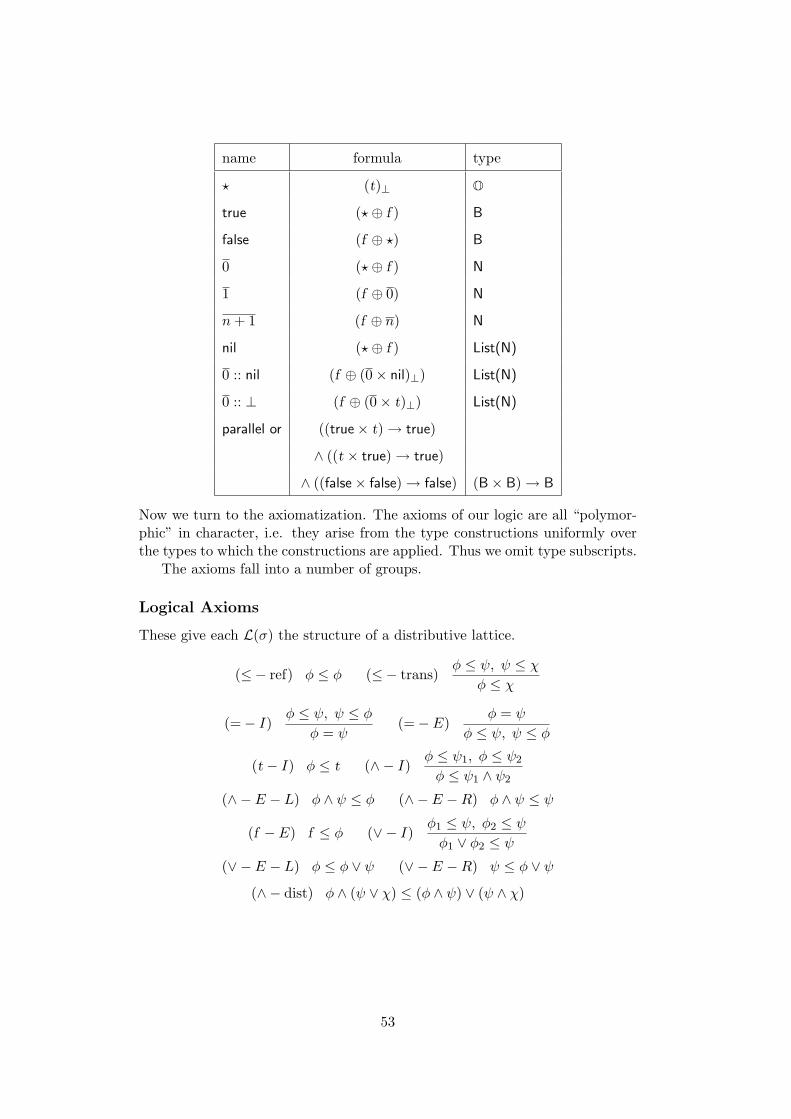
name formula type

? (t)⊥ O

true (?⊕ f ) B

false (f ⊕ ?) B

0 (?⊕ f ) N

1 (f ⊕ 0) N

n+ 1 (f ⊕ n) N

nil (?⊕ f ) List(N)

0 :: nil (f ⊕ (0× nil)⊥) List(N)

0 :: ⊥ (f ⊕ (0× t)⊥) List(N)

parallel or ((true× t)→ true)

∧ ((t × true)→ true)

∧ ((false× false)→ false) (B× B)→ B

Now we turn to the axiomatization. The axioms of our logic are all “polymor-phic” in character, i.e. they arise from the type constructions uniformly overthe types to which the constructions are applied. Thus we omit type subscripts.

The axioms fall into a number of groups.

Logical Axioms

These give each L(σ) the structure of a distributive lattice.

(≤− ref) φ ≤ φ (≤− trans)φ ≤ ψ, ψ ≤ χ

φ ≤ χ

(=− I) φ ≤ ψ, ψ ≤ φφ = ψ

(=− E)φ = ψ

φ ≤ ψ, ψ ≤ φ

(t − I) φ ≤ t (∧ − I) φ ≤ ψ1, φ ≤ ψ2

φ ≤ ψ1 ∧ ψ2

(∧ − E − L) φ ∧ ψ ≤ φ (∧ − E −R) φ ∧ ψ ≤ ψ

(f − E) f ≤ φ (∨ − I) φ1 ≤ ψ, φ2 ≤ ψφ1 ∨ φ2 ≤ ψ

(∨ − E − L) φ ≤ φ ∨ ψ (∨ − E −R) ψ ≤ φ ∨ ψ

(∧ − dist) φ ∧ (ψ ∨ χ) ≤ (φ ∧ ψ) ∨ (ψ ∧ χ)

53

Type-specific Axioms

These articulate each type construction, by showing how its generators interactwith the logical structure.

(×− ∧)∧

i∈I(φi × ψi) = (∧

i∈I φi ×∧

i∈I ψi)

(×− ∨− L) (∨

i∈I φi × ψ) =∨

i∈I(φ× ψ)

(×− ∨−R) (φ×∨

i∈I ψi) =∨

i∈I(φ× ψi)

(→−∧) (φ→∧

i∈I ψi) =∧

i∈I(φ→ ψi)

(→−∨− L) (∨

i∈I φi → ψ) =∧

i∈I(φi → ψ)

(⊕− ∧− L) (∧

i∈I φi ⊕ f ) =∧

i∈I(φi ⊕ f )

(⊕− ∧−R) (f ⊕∧

i∈I ψi) =∧

i∈I(f ⊕ ψi)

(⊕− ∨− L) (∨

i∈I φi ⊕ f ) =∨

i∈I(φi ⊕ f )

(⊕− ∨−R) (f ⊕∨

i∈I ψi) =∨

i∈I(f ⊕ ψi)

((·)⊥ − ∧) (φ ∧ ψ)⊥ = (φ)⊥ ∧ (ψ)⊥

((·)⊥ − ∨) (∨

i∈I φi)⊥ =∨

i∈I(φi)⊥

(2− ∧) 2∧

i∈I φi =∧

i∈I 2φi

(3− ∨) 3∨

i∈I φi =∨

i∈I 3φi

(2− ∨) 2(φ ∨ ψ) ≤ 2φ ∨3ψ

(3− ∧) 2φ ∧3ψ ≤ 3(φ ∧ ψ)

(2− f ) 2f = f

Rules

(→−∨−R)C(φ)

(φ→∨

i∈I ψi) =∨

i∈I(φ→ ψi)

(⊕−#)T(φ) T(ψ)

(φ⊕ f ) ∧ (f ⊕ ψ) = f

(×−≤)φ ≤ φ′, ψ ≤ ψ′

(φ× ψ) ≤ (φ′ × ψ′)

(→− ≤)φ′ ≤ φ, ψ ≤ ψ′

(φ→ ψ) ≤ (φ′ → ψ′)

(⊕−≤)φ ≤ ψ

(φ⊕ f ) ≤ (ψ ⊕ f ), (f ⊕ φ) ≤ (f ⊕ ψ)

((·)⊥ −≤)φ ≤ ψ

(φ)⊥ ≤ (ψ)⊥

(2−≤)φ ≤ ψ

2φ ≤ 2ψ(3−≤)

φ ≤ ψ3φ ≤ 3ψ

54

Generic Axioms for Coprimeness and Termination

(C −=)C(φ), φ = ψ

C(ψ)(C − t) C(t)

(T −≤)T(φ), ψ ≤ φ

T(ψ)(T − ∧)

T(φj) (j ∈ I)T(

∧i∈I φi)

(T − ∨)T(φi)i∈I

T(∨

i∈I φi)

Type-Specific Axioms for Coprimeness

(C −×)C(φ) C(ψ)C(φ× ψ)

(C −→)

C(φi)i∈I C(ψi)i∈I

∀J ⊆ I.∃K ⊆ I. [∧

j∈J φj =∨

k∈K φk & [∀j ∈ J, k ∈ K.ψk ≤ ψj ]]

C(∧

i∈I(φi → ψi))

(C −⊕)C(φ)

C(φ⊕ f )C(ψ)

C(f ⊕ ψ)(C − (·)⊥)

C(φ)C((φ)⊥)

(C −2−3)C(φi)i∈I (I 6= ∅)

C(2∨

i∈I φi ∧∧

i∈I 3φi)

Type-Specific Axioms for Termination

(T −×)T(φ)

T(φ× ψ)T(ψ)

T(φ× ψ)

(T −→)C(φ′) φ′ ≤ φ T(ψ)

T(φ→ ψ)

(T −⊕)T(φ)

T(φ⊕ f )T(ψ)

T(f ⊕ ψ)

(T − (·)⊥) T((φ)⊥)

(T −2)T(φ)

T(2φ)(T −3)

T(φ)T(3φ)

Remarks on the Axiomatization

The above axioms and rules are to be understood as schemes, which are instan-tiated by uniform substitution for meta-variables. A literal is one of the basicassertions φ ≤ ψ, φ = ψ, C(φ), T(φ). All our rules have the form: “from afinite conjunction of literals (empty in the case of an axiom) infer a literal”, i.e.∧

i∈I

li ⇒ l

55

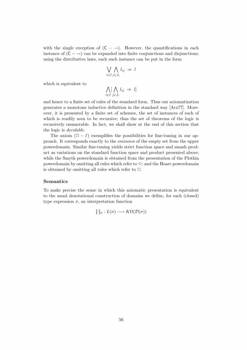
with the single exception of (C − →). However, the quantifications in eachinstance of (C −→) can be expanded into finite conjunctions and disjunctions;using the distributive laws, each such instance can be put in the form∨

i∈I

∧j∈Ji

lij ⇒ l

which is equivalent to ∧i∈I

[∧

j∈Ji

lij ⇒ l]

and hence to a finite set of rules of the standard form. Thus our axiomatizationgenerates a monotone inductive definition in the standard way [Acz77]. More-over, it is presented by a finite set of schemes, the set of instances of each ofwhich is readily seen to be recursive; thus the set of theorems of the logic isrecursively enumerable. In fact, we shall show at the end of this section thatthe logic is decidable.

The axiom (2 − f ) exemplifies the possibilities for fine-tuning in our ap-proach. It corresponds exactly to the omission of the empty set from the upperpowerdomain. Similar fine-tuning yields strict function space and smash prod-uct as variations on the standard function space and product presented above;while the Smyth powerdomain is obtained from the presentation of the Plotkinpowerdomain by omitting all rules which refer to 3; and the Hoare powerdomainis obtained by omitting all rules which refer to 2.

Semantics

To make precise the sense in which this axiomatic presentation is equivalentto the usual denotational construction of domains we define, for each (closed)type expression σ, an interpretation function

[[·]]σ : L(σ) −→ KΩ(D(σ))

56

by

[[φ ∧ ψ]]σ = [[φ]]σ ∩ [[ψ]]σ

[[t]]σ = D(σ) = 1KΩ(D(σ))

[[φ ∨ ψ]]σ = [[φ]]σ ∪ [[ψ]]σ

[[f ]]σ = ∅ = 0KΩ(D(σ))

[[(φ× ψ)]]σ×τ = 〈u, v〉 : u ∈ [[φ]]σ, v ∈ [[ψ]]τ

[[(φ→ ψ)]]σ→τ = f ∈ D(σ → τ) : f([[φ]]σ) ⊆ [[ψ]]τ

[[(φ⊕ f )]]σ⊕τ = 〈0, u〉 : u ∈ [[φ]]σ \ ⊥σ

∪ d ∈ D(σ ⊕ τ) : ⊥σ ∈ [[φ]]σ

[[(f ⊕ ψ)]]σ⊕τ = 〈1, v〉 : v ∈ [[ψ]]τ \ ⊥τ

∪ d ∈ D(σ ⊕ τ) : ⊥τ ∈ [[ψ]]τ

[[(φ)⊥]](σ)⊥ = 〈0, u〉 : u ∈ [[φ]]σ

[[2φ]]Pσ = S ∈ D(Pσ) : S ⊆ [[φ]]σ

[[3φ]]Pσ = S ∈ D(Pσ) : S ∩ [[φ]]σ 6= ∅

[[φ]]rec t. σ = ασ(u) : u ∈ [[φ]]σ[rec t. σ/t]

where ασ : D(σ[rec t. σ/t]) ∼= D(rec t. σ) is the isomorphism arising from theinitial solution to the domain equation t = σ(t).

Then for φ, ψ ∈ L(σ), we define

D(σ) |= φ ≤ ψ ≡ [[φ]]σ ⊆ [[ψ]]σ.

We now use the results of Chapter 3 to establish some fundamental proper-ties of our system of “Domain Logic”.

Firstly, we note that operations on domain prelocales in the style of Chap-ter 3 can be distilled from our definitions for product and lifting. The readerwill find no difficulty in carrying out the same programme for these construc-tions as that shown for function space, Plotkin powerdomain and coalesced sumin Chapter 3. It is immediate from the definitions that, for each closed σ andany ρ ∈ LEnv:

L(σ) = L[[σ]]ρ

where L[[σ]]ρ is the logical semantics from Section 3.5. The following results arethen immediate consequences of our work in Chapter 3.Notation. C(σ) ≡ φ ∈ L(σ) : L(σ) ` C(φ).

Lemma 4.2.1 (Normal Forms) For all φ ∈ L(σ), for some ψi, . . . , ψn ∈C(σ):

L(σ) ` φ =n∨

i=1

ψi.

57

Now we define a relation ! ⊆ C(σ)×K(D(σ)):

φ ! u ≡ [[φ]]σ = ↑(u).

Proposition 4.2.2 ! is a surjective total function.

Now we come to the main results of the section:

Theorem 4.2.3 (Soundness and Completeness) For all φ, ψ ∈ L(σ):

L(σ) ` φ ≤ ψ ⇐⇒ D(σ) |= φ ≤ ψ.

Now we defineLA(σ) ≡ (L(σ)/=σ, ≤σ /=σ),

the Lindenbaum algebra of L(σ).

Theorem 4.2.4 (Stone Duality) LA(σ) is the Stone dual of D(σ), i.e.

(i) D(σ) ∼= Spec LA(σ)

(ii) KΩ(D(σ)) ∼= LA(σ).

Decidability of L

We define a set T of formulae in L by the following syntax:

φ ::= t | (φ× ψ) |∧i∈I

(φi → ψi) | (φ⊕ f ) | (f ⊕ ψ) | (φ)⊥ | 2∨i∈I

φi ∧∧i∈I

3φi.

A formula φ is a rigid coprime if φ ∈ T and L ` C(φ); a formula is in rigidcoprime normal form if it is a disjunction of rigid coprimes.

We now define predicates LEQ, TERM over rigid coprimes (of the sametype in the case of LEQ), by the following inductive definitions:

• LEQ(φ, t) ⇐⇒ true

• LEQ(t, φ) ⇐⇒ ¬(TERM(φ))

• LEQ((φ× ψ), (φ′ × ψ′)) ⇐⇒ LEQ(φ, φ′) & LEQ(ψ,ψ′)

• LEQ(∧

i∈I(φi → ψi),∧

j∈J(φj → ψj)) ⇐⇒ ∀j ∈ J.∃i ∈ I.

LEQ(φj , φi) & LEQ(ψi, ψj)

• LEQ((φ⊕ f ), (φ′ ⊕ f )) ⇐⇒ LEQ(φ, φ′)

• LEQ((φ⊕ f ), (f ⊕ ψ)) ⇐⇒ LEQ(t, ψ)

• LEQ((f ⊕ ψ), (f ⊕ ψ′)) ⇐⇒ LEQ(ψ,ψ′)

• LEQ((f ⊕ ψ), (φ⊕ f )) ⇐⇒ LEQ(t, φ)

• LEQ((φ)⊥, (ψ)⊥) ⇐⇒ LEQ(φ, ψ)

• LEQ(2∨

i∈I φi ∧∧

i∈I 3φi,

2∨

j∈J ψj ∧∧

j∈J 3ψj) ⇐⇒ ∀i ∈ I.∃j ∈ J.LEQ(φi, ψj)

& ∀j ∈ J.∃i ∈ I.LEQ(φi, ψj)

58

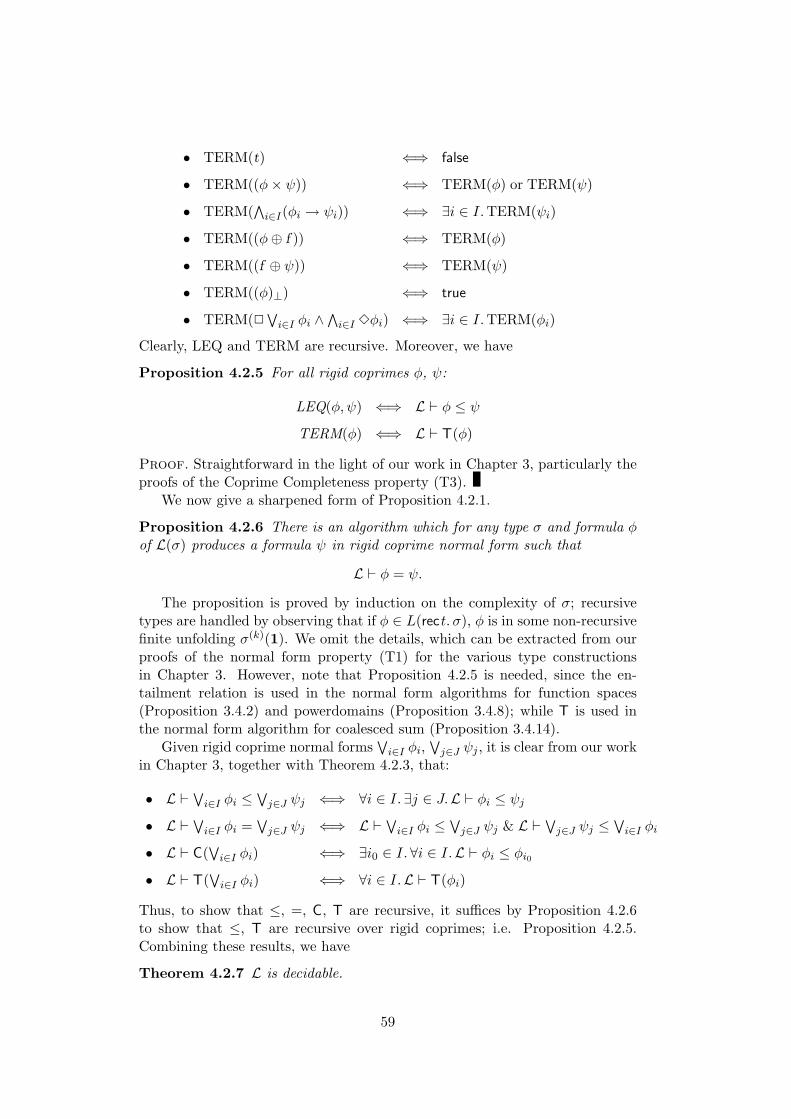
• TERM(t) ⇐⇒ false

• TERM((φ× ψ)) ⇐⇒ TERM(φ) or TERM(ψ)

• TERM(∧

i∈I(φi → ψi)) ⇐⇒ ∃i ∈ I.TERM(ψi)

• TERM((φ⊕ f )) ⇐⇒ TERM(φ)

• TERM((f ⊕ ψ)) ⇐⇒ TERM(ψ)

• TERM((φ)⊥) ⇐⇒ true

• TERM(2∨

i∈I φi ∧∧

i∈I 3φi) ⇐⇒ ∃i ∈ I.TERM(φi)

Clearly, LEQ and TERM are recursive. Moreover, we have

Proposition 4.2.5 For all rigid coprimes φ, ψ:

LEQ(φ, ψ) ⇐⇒ L ` φ ≤ ψ

TERM(φ) ⇐⇒ L ` T(φ)

Proof. Straightforward in the light of our work in Chapter 3, particularly theproofs of the Coprime Completeness property (T3).

We now give a sharpened form of Proposition 4.2.1.

Proposition 4.2.6 There is an algorithm which for any type σ and formula φof L(σ) produces a formula ψ in rigid coprime normal form such that

L ` φ = ψ.

The proposition is proved by induction on the complexity of σ; recursivetypes are handled by observing that if φ ∈ L(rect. σ), φ is in some non-recursivefinite unfolding σ(k)(1). We omit the details, which can be extracted from ourproofs of the normal form property (T1) for the various type constructionsin Chapter 3. However, note that Proposition 4.2.5 is needed, since the en-tailment relation is used in the normal form algorithms for function spaces(Proposition 3.4.2) and powerdomains (Proposition 3.4.8); while T is used inthe normal form algorithm for coalesced sum (Proposition 3.4.14).

Given rigid coprime normal forms∨

i∈I φi,∨

j∈J ψj , it is clear from our workin Chapter 3, together with Theorem 4.2.3, that:

• L `∨

i∈I φi ≤∨

j∈J ψj ⇐⇒ ∀i ∈ I.∃j ∈ J.L ` φi ≤ ψj

• L `∨

i∈I φi =∨

j∈J ψj ⇐⇒ L `∨

i∈I φi ≤∨

j∈J ψj & L `∨

j∈J ψj ≤∨

i∈I φi

• L ` C(∨

i∈I φi) ⇐⇒ ∃i0 ∈ I.∀i ∈ I.L ` φi ≤ φi0

• L ` T(∨

i∈I φi) ⇐⇒ ∀i ∈ I.L ` T(φi)

Thus, to show that ≤, =, C, T are recursive, it suffices by Proposition 4.2.6to show that ≤, T are recursive over rigid coprimes; i.e. Proposition 4.2.5.Combining these results, we have

Theorem 4.2.7 L is decidable.

59

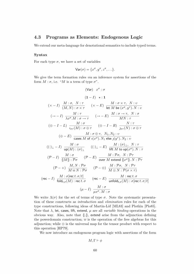
4.3 Programs as Elements: Endogenous Logic

We extend our meta-language for denotational semantics to include typed terms.

Syntax

For each type σ, we have a set of variables

Var(σ) = xσ, yσ, zσ, . . ..

We give the term formation rules via an inference system for assertions of theform M : σ, i.e. “M is a term of type σ”.

(Var) xσ : σ

(1− I) ? : 1

(×− I) M : σ, N : τ(M,N) : σ × τ

(×− E)M : σ × τ, N : υ

let M be (xσ, yτ ). N : υ

(→− I) M : τλxσ.M : σ → τ

(→− E)M : σ → τ, N : σ

MN : τ

(⊕− I − L)M : σ

ıστ (M) : σ ⊕ τ(⊕− I −R)

N : τστ (N) : σ ⊕ τ

(⊕− E)M : σ ⊕ τ, N1, N2 : υ

cases M of ı(xσ). N1 else (yτ ). N2 : υ

((·)⊥ − I)M : σ

up(M) : (σ)⊥((·)⊥ − E)

M : (σ)⊥, N : τlift M to up(xσ). N : τ

(P − I) M : σ|M | : Pσ

(P − E)M : Pσ, N : Pτ

over M extend |xσ|. N : Pτ

(P −+)M,N : PσM ]N : Pσ

(P −⊗)M : Pσ, N : PτM ⊗N : P(σ × τ)

(rec− I) M : σ[rec t. σ/t]foldt,σ(M) : rec t. σ

(rec− E)M : rec t. σ

unfoldt,σ(M) : σ[rec t. σ/t]

(µ− I) M : σµxσ.M : σ

We write Λ(σ) for the set of terms of type σ. Note the systematic presenta-tion of these constructs as introduction and elimination rules for each of thetype constructions, following ideas of Martin-Lof [ML83] and Plotkin [Plo85].Note that λ, let, cases, lift, extend, µ are all variable binding operations in theobvious way. Also, note that |.|, extend arise from the adjunction definingthe powerdomain construction; ] is the operation of the free algebras for thisadjunction; while ⊗ is the universal map for the tensor product with respect tothis operation [HP79].

We now introduce an endogenous program logic with assertions of the form

M,Γ ` φ

60

where M : σ, φ ∈ L(σ), and Γ ∈∏

σVar(σ)→ L(σ) gives assumptions on thefree variables of M .Notation

Γ ≤ ∆ ≡ ∀x ∈ Var.L ` Γx ≤ ∆x.

For the remainder of this Chapter, we shall omit type subscripts and super-scripts “whenever [we think]2 we can get away with it”, in the delightful for-mulation of Barr and Wells [BW84, p. 1].

Axiomatisation

(` − ∧)M,Γ ` φii∈I

M,Γ `∧

i∈I φi(` − ∨)

M,Γ[x 7→ φi] ` ψi∈I

M,Γ[x 7→∨

i∈I φi] ` ψ

(` − ≤)Γ ≤ ∆ M,∆ ` φ φ ≤ ψ

M,Γ ` ψx,Γ[x 7→ φ] ` φ

M,Γ ` φ N,Γ ` ψ(M,N),Γ ` (φ× ψ)

M,Γ ` (φ× ψ) N,Γ[x 7→ φ, y 7→ ψ] ` θlet M be (x, y). N,Γ ` θ

M,Γ[x 7→ φ] ` ψλx.M,Γ ` (φ→ ψ)

M,Γ ` (φ→ ψ) N,Γ ` φMN,Γ ` ψ

M,Γ ` φı(M),Γ ` (φ⊕ f )

M,Γ ` (φ⊕ f ) T(φ) N1,Γ[x 7→ φ] ` θcases M of ı(x). N1 else (y). N2,Γ ` θ

N,Γ ` ψ(N),Γ ` (f ⊕ ψ)

M,Γ ` (f ⊕ ψ) T(ψ) N2,Γ[y 7→ ψ] ` θcases M of ı(x). N1 else (y). N2,Γ ` θ

M,Γ ` φup(M),Γ ` (φ)⊥

M,Γ ` (φ)⊥ N,Γ[x 7→ φ] ` ψlift M to up(x). N,Γ ` ψ

M,Γ ` φ|M |,Γ ` 3φ

M,Γ ` φ|M |,Γ ` 2φ

M,Γ ` 3φ N,Γ[x 7→ φ] ` 3ψ

over M extend |x|. N,Γ ` 3ψ

M,Γ ` 2φ N,Γ[x 7→ φ] ` 2ψ

over M extend |x|. N,Γ ` 2ψ

M,Γ ` 3φ

M ]N,Γ ` 3φ

N,Γ ` 3ψ

M ]N,Γ ` 3ψ

M,Γ ` 2φ N,Γ ` 2φ

M ]N,Γ ` 2φ

M,Γ ` 3φ N,Γ ` 3ψ

M ⊗N,Γ ` 3(φ× ψ)M,Γ ` 2φ N,Γ ` 2ψ

M ⊗N,Γ ` 2(φ× ψ)

M,Γ ` φfold(M),Γ ` φ

M,Γ ` φunfold(M),Γ ` φ

µx.M,Γ ` φ M,Γ[x 7→ φ] ` ψµx.M,Γ ` ψ

Note that there is one inference rule for ` per formation rule in our syntax.Thus we can refer e.g. to rule (` − × − E) without ambiguity. (In the case ofthe powerdomain constructions, we have one rule each for box and diamond,

2Inserted by the author.

61

and refer e.g. to (` −2− I)). Note the role of the termination predicate T in(`−⊕−E); it plays a similar role in the elimination rules for the other “strict”constructions of smash product [Plo81, Chapter 3 p. 1] and strict function space[Plo81, Chapter 1 p. 11], which we do not cover here.

Also, note the resemblance of our system to type inference (particularly tothe conjunctive type discipline of [BCDC83, CDCHL84]); this stands out evenmore clearly if we use the notation

Γ `M : φ

for assertions. One can profitably think of properties φ as “local types”, ina richer type system (powerdomains, lifting, recursive types) than is usuallyconsidered.

Semantics

Following standard ideas [Plo81, SP82, Plo76], we now give a denotational se-mantics for this meta-language, in the form of a map

[[·]]σ : Λ(σ) −→ Env −→ D(σ)

where Env ≡∏

σVar(σ)→ D(σ) is the set of environments.

[[x]]ρ = ρx

[[(M,N)]]ρ = 〈[[M ]]ρ, [[N ]]ρ〉

[[let M be (x, y). N ]]ρ = [[N ]]ρ[x 7→ d, y 7→ e]

where

〈d, e〉 = [[M ]]ρ

[[λx.M ]]ρ = (d 7→ [[M ]]ρ[x 7→ d])

[[MN ]]ρ = ([[M ]]ρ)([[N ]]ρ)

[[ı(M)]]ρ =

〈0, [[M ]]ρ〉, [[M ]]ρ 6= ⊥

⊥ [[M ]]ρ = ⊥

[[(N)]]ρ =

〈1, [[N ]]ρ〉, [[N ]]ρ 6= ⊥

⊥ [[N ]]ρ = ⊥

[[cases M of

ı(x). N1 else (y). N2]]ρ =

[[N1]]ρ[x 7→ d], [[M ]]ρ = 〈0, d〉

[[N2]]ρ[y 7→ e], [[M ]]ρ = 〈1, e〉

⊥, [[M ]]ρ = ⊥

[[up(M)]]ρ = 〈0, [[M ]]ρ〉

[[lift M to up(x). N ]]ρ =

[[N ]]ρ[x 7→ d], [[M ]]ρ = 〈0, d〉

⊥, [[M ]]ρ = ⊥

62

[[|M |]]ρ = [[M ]]ρ

[[over M extend |x|. N ]]ρ = ↑(X) ∩ X,

where X =⋃[[N ]]ρ[x 7→ d] : d ∈ [[M ]]ρ

[[M ]N ]]ρ = Con(([[M ]]ρ) ∪ ([[N ]]ρ))

[[M ⊗N ]]ρ = Con(([[M ]]ρ)× ([[N ]]ρ))

[[fold(M)]]ρ = α([[M ]]ρ)

[[unfold(M)]]ρ = α−1([[M ]]ρ)

[[µx.M ]]ρ =⊔

k∈ω dk

where d0 = ⊥, dk+1 = [[M ]]ρ[x 7→ dk]

Here α is the initial algebra isomorphism as in Section 2 page 57.We can use this semantics to define a notion of validity for assertions:

M,Γ |= φ ≡ ∀ρ ∈ Env. ρ |= Γ⇒ [[M ]]σρ |= φ

whereρ |= Γ ≡ ∀x ∈ Var. ρx |= Γx

and for d ∈ D(σ), φ ∈ L(σ):

d |= φ ≡ d ∈ [[φ]]σ.

We can now state the main result of this section:

Theorem 4.3.1 The Endogenous logic is sound and complete:

∀M,Γ, φ. M,Γ ` φ ⇐⇒ M,Γ |= φ.

We can state this result more sharply in terms of Stone Duality: for closedσ and M it says that, for any ρ and Γ:

η−1σ ([φ]=σ : M,Γ ` φ) = [[M ]]σρ,

whereησ : D(σ) ∼= Spec(LA(σ))

is the component of the natural isomorphism arising from Theorem 4.2.4; i.e.that we recover the point of D(σ) given by the denotational semantics of Mfrom the properties we can prove to hold of M in our logic.

We now turn to the proof of Theorem 4.3.1. Our strategy is analogous tothat of Chapter 3; we get Completeness via Coprime Completeness. Firstly, wehave:

Theorem 4.3.2 (Soundness) For all M , Γ, φ:

M,Γ ` φ =⇒ M,Γ |= φ.

63

Proof. By a routine induction on the length of proofs in the endogenous logic.We give two cases for illustration.1. Suppose the last step in the proof is an application of (` −→− I):

M,Γ[x 7→ φ] ` ψλx.M,Γ ` (φ→ ψ)

By induction hypothesis, M,Γ[x 7→ φ] |= ψ, i.e for all ρ |= Γ, d ∈ D(σ),

d ∈ [[φ]] =⇒ [[M ]]ρ[x 7→ d] ∈ [[ψ]],

which impliesλx.M,Γ |= (φ→ ψ).

2. Next we consider (` −2− E):

M,Γ ` 2φ N,Γ[x 7→ φ] ` 2ψ

over M extend |x|. N,Γ ` 2ψ

By induction hypothesis, M,Γ |= 2φ and N,Γ[x 7→ φ] |= 2ψ. Hence for ρ |= Γ,[[M ]]ρ ⊆ [[φ]], and for d ∈ D(σ),

d ∈ [[φ]] =⇒ [[N ]]ρ[x 7→ d] ⊆ [[ψ]].

Thus• X =

⋃d∈[[M ]]ρ[[N ]]ρ[x 7→ d] ⊆ [[ψ]]

=⇒ [[over M extend |x|. N ]]ρ ⊆ ↑(X) ⊆ [[ψ]]

=⇒ over M extend |x|. N,Γ |= 2ψ.

Next, we shall need a technical lemma which describes our program con-structs under the denotational semantics.

Lemma 4.3.3 For u ∈ K(D(σ)), v ∈ K(D(τ)), w ∈ K(D(υ)), X ∈ ℘fne(K(D(σ))),

64

Y ∈ ℘fne(K(D(τ))), Z ∈ ℘fne(K(D(σ×τ))), w1 ∈ K(D(rect. σ)), w2 ∈ K(D(σ[rect. σ/t])):

(i) (u, v) v [[(M,N)]]ρ ⇔ u v [[M ]]ρ& v v [[N ]]ρ

(ii) w v [[let M be (x, y). N ]]ρ ⇔ ∃u, v.

(u, v) v [[M ]]ρ& w v [[N ]]ρ[x 7→ u, y 7→ v]

(iii) (uv) v [[λx.M ]]ρ ⇔ v v [[M ]]ρ[x 7→ u]

(iv) v v [[MN ]]ρ ⇔ ∃u.(uv) v [[M ]]ρ& u v [[N ]]ρ

(v) 〈0, u〉 v [[ı(M)]]ρ ⇔ u v [[M ]]ρ

〈1, v〉 v [[(N)]]ρ ⇔ v v [[N ]]ρ

(vi) w 6= ⊥ =⇒ w v [[cases M of ı(x). N1 else (y). N2]]ρ ⇔

∃u 6= ⊥. 〈0, u〉 v [[M ]]ρ& w v [[N1]]ρ[x 7→ u]

or

∃v 6= ⊥. 〈1, v〉 v [[M ]]ρ& w v [[N2]]ρ[x 7→ v]

(vii) 〈0, u〉 v [[up(M)]]ρ ⇔ u v [[M ]]ρ

(viii) v 6= ⊥ =⇒ v v [[lift M to up(x). N ]]ρ ⇔

∃u. 〈0, u〉 v [[M ]]ρ& v v [[N ]]ρ[x 7→ u]

(ix) Con(X) v [[|M |]]ρ ⇔ ∀x ∈ X.x v [[M ]]ρ

(x) Con(Y ) v [[over M extend |x|. N ]]ρ ⇔ ∃X.Con(X) v [[M ]]ρ

& Con(Y ) v Con(⋃

u∈X [[N ]]ρ[x 7→ u])

(xi) Con(X) v [[M ]N ]]ρ ⇔ ∃Y, Z.Con(X) = Con(Y ∪ Z)

& Con(Y ) v [[M ]]ρ & Con(Z) v [[N ]]ρ

(xii) Con(Z) v [[M ⊗N ]]ρ ⇔ ∃X,Y. Con(Z) v Con(X)⊗ Con(Y )

& Con(X) v [[M ]]ρ & Con(Y ) v [[N ]]ρ

(xiii) w1 v [[fold(M)]]ρ ⇔ α−1(w1) v [[M ]]ρ

(xiv) w2 v [[unfold(M)]]ρ ⇔ α(w2) v [[M ]]ρ

(xv) u v [[µx.M ]]ρ ⇔ ∃k ∈ ω, u0, . . . , uk. u0 = ⊥& uk = u

& ∀i : 0 ≤ i < k. ui+1 v [[M ]]ρ[x 7→ ui]

Proof. The content of this Lemma is all quite standard, at least in the folklore.It amounts to a description of the combinators underlying the denotational se-mantics of terms as approximable mappings. Most of it can be found, couched inthe language of information systems, in [Sco82], and for neighbourhood systemsin [Sco81]. See also [Gun85]. We shall just give a couple of the less familiarcases for illustration.

65

(xi).

• Con(X) v [[M ]N ]]ρ

⇐⇒ X vEM ([[M ]]ρ ∪ [[N ]]ρ)

⇐⇒ Con(Y ) v [[M ]]ρ & Con(Z) v [[N ]]ρ

whereY = y ∈ X : ∃x ∈ [[M ]]ρ. y v x

Z = z ∈ X : ∃x ∈ [[N ]]ρ. y v x.

(xii).

• Con(Z) v [[M ⊗N ]]ρ

⇐⇒ Con(Z) v⊔Con(X)⊗ Con(Y ) : Con(X) v [[M ]]ρ& Con(Y ) v [[N ]]ρ

since ⊗ is continuous

⇐⇒ ∃X,Y. Con(Z) v Con(X)⊗ Con(Y ) & Con(X) v [[M ]]ρ & Con(Y ) v [[N ]]ρ

since Con(Z) is finite.

Now for Coprime Completeness.Notation. C(Γ) ≡ ∀x ∈ Var.C(Γx).

Theorem 4.3.4 (Coprime Completeness) C(Γ) and C(φ) imply that

M,Γ |= φ =⇒ M,Γ ` φ

Proof. We begin by establishing some useful notation. Given Γ with C(Γ), wedefine an environment ρΓ by:

∀x ∈ Var.Γx ! ρΓx.

This is well-defined by Proposition 4.2.2. Similarly, let φ ! u. Now we have:

M,Γ |= φ ⇐⇒ u v [[M ]]ρΓ. (4.1)

The proof proceeds by induction on M . As the various cases all share a commonpattern, we shall only give a selection of the more interesting for illustration.

Abstraction. We argue by induction on the proof that C(φ). The non-trivialcase is when this is inferred by (C−→), with φ =

∧i∈I(φi → ψi). Let φi ! ui,

66

ψi ! vi, i ∈ I. Then

• λx.M,Γ |= φ

⇒ ∀i ∈ I. λx.M,Γ |= (φi → ψi)

⇒ ∀i ∈ I. (uivi) v [[λx.M ]]ρΓ (4.1)

⇒ ∀i ∈ I. vi v [[M ]]ρΓ[x 7→ ui] 4.3.3(iii)

⇒ ∀i ∈ I.M,Γ[x 7→ φi] |= ψi (4.1)

⇒ ∀i ∈ I.M,Γ[x 7→ φi] ` ψi ind. hyp.

⇒ ∀i ∈ I. λx.M,Γ ` (φi → ψi) (` −→− I)

⇒ λx.M,Γ ` φ (` − ∧).

Application.

• MN,Γ |= φ

⇒ u v [[MN ]]ρΓ (4.1)

⇒ ∃v. (vu) v [[M ]]ρ& v v [[N ]]ρ 4.3.3(iv)

⇒ M,Γ |= (ψ → φ) & N,Γ |= ψ (4.1)

where ψ ! v

⇒ M,Γ ` (ψ → φ) & N,Γ ` ψ ind. hyp.

⇒ MN,Γ ` φ (` −→− E).

Case expression.

cases M of ı(x). N1 else (y). N2,Γ |= φ

⇔ u v [[cases M of ı(x). N1 else (y). N2]]ρΓ (4.1).

If u = ⊥, then L ` t ≤ φ, and the required conclusion follows by (` − ∧) and(` − ≤). Otherwise, by 4.3.3(vi), either

(i) ∃u1 6= ⊥. 〈0, u1〉 v [[M ]]ρΓ & u v [[N1]]ρΓ[x 7→ u1]

or(ii) ∃u2 6= ⊥. 〈1, u2〉 v [[M ]]ρΓ & u v [[N2]]ρΓ[x 7→ u2].

We shall consider sub-case (i); (ii) is entirely similar. Let φ1 ! u1. Then

• 〈0, u1〉 v [[M ]]ρΓ & u v [[N1]]ρΓ[x 7→ u1]

⇒ M,Γ |= (φ1 ⊕ f ) & N1,Γ[x 7→ φ1] |= φ (4.1)

⇒ M,Γ ` (φ1 ⊕ f ) & N1,Γ[x 7→ φ1] ` φ ind. hyp.

⇒ cases M of ı(x). N1 else (y). N2,Γ ` φ by (` − ⊕− E)

since u1 6= ⊥ implies T(φ1).

67

Tensor product. By induction on the proof that C(φ). The non-trivial caseis when this is inferred by (C −2−3), with

φ = 2∨i∈I

(φi × ψi) ∧∧i∈I

3(φi × ψi)

with C(φi), C(ψi), i ∈ I. We define Z = (ui, vi) : i ∈ I, where

φi ! ui, ψi ! vi (i ∈ I).

Now

• M ⊗N,Γ |= 2∨

i∈I(φ× ψ) ∧∧

i∈I 3(φi × ψi)

⇒ Con(Z) v [[M ⊗N ]]ρΓ (4.1)

⇒ ∃X,Y. Con(X) v [[M ]]ρΓ & Con(Y ) v [[N ]]ρΓ

& Con(Z) v Con(X)⊗ Con(Y ) = Con(X × Y ) 4.3.3(xii)

Let X = ukk∈K , Y = vll∈L, and define

φk ! uk (k ∈ K), ψl ! vl (l ∈ L).

Now

• Con(X) v [[M ]]ρΓ & Con(Y ) v [[N ]]ρΓ

⇒ M,Γ |= 2∨

k∈K φk ∧∧

k∈K 3φk & N,Γ |= 2∨

l∈L ψl ∧∧

l∈L 3ψl (4.1)

⇒ M,Γ ` 2∨

k∈K φk ∧∧

k∈K 3φk & N,Γ ` 2∨

l∈L ψl ∧∧

l∈L 3ψl ind. hyp.

⇒ M ⊗N,Γ ` 2(∨

k∈K φk ×∨

l∈L ψ) ∧∧

(k,l)∈K×L 3(φk × ψl) (` − ⊗).

Now Con(Z) v Con(X)⊗ Con(Y ) implies

∀(k, l).∃i. L ` (φk × ψl) ≤ (φi × ψi) & ∀i. ∃(k, l). L ` (φk × ψl) ≤ (φi × ψi).

Hence

L ` (∨

k∈K φk ×∨

l∈L ψl) =∨

(k,l)∈K×L(φk × ψl) (×− ∨)

≤∨

i∈I(φi × ψi)

and so by (2−≤),

L ` 2(∨

k∈K

φk ×∨l∈L

ψl) ≤ 2∨i∈I

(φi × ψi).

Again, by (3−≤), for all i, for some (k, l):

L ` 3(φk × ψl) ≤ 3(φi × ψi)

and soL `

∧(k,l)∈K×L

3(φk × ψl) ≤∧i∈I

3(φi × ψi).

68

Hence by (` − ≤),M ⊗N,Γ ` φ.

Recursive types. Firstly, we note that for φ ∈ L(rec t. σ),

φ ! u ⇔ φ ! α−1(u),

since L(rec t. σ) = L(σ[rec t. σ/t]). Now,

• fold(M),Γ |= φ

⇒ u v [[fold(M)]]ρΓ (4.1)

⇒ α−1(u) v [[M ]]ρΓ 4.3.3(xiii)

⇒ M,Γ |= φ (4.1)

⇒ M,Γ ` φ ind. hyp.

⇒ fold(M),Γ ` φ (` − rec− I)

Recursion.

• µx.M,Γ |= φ

⇒ u v [[µx.M ]]ρΓ (4.1)

⇒ ∃k ∈ ω, u0, . . . , uk. u0 = ⊥& uk = u

& ∀i : 0 ≤ i < k. ui+1 v [[M ]]ρΓ[x 7→ ui] 4.3.3(xv).

Let ‖u‖ be the least such k (as a function of u for u v [[µx.M ]]ρΓ, keepingµx.M , Γ fixed). We complete the proof for this case by induction on ‖u‖, withφ ! u.

Basis:‖u‖ = 0⇒ u = ⊥ ⇒ ` t ≤ φ⇒ µx.M,Γ ` φ,

by (` − ∧) and (` − ≤).Induction step: ‖u‖ = k + 1. Then by definition of ‖u‖, for some v:

u v [[M ]]ρΓ[x 7→ v] & ‖v‖ = k.

Let ψ ! v. Then

• u v [[M ]]ρΓ[x 7→ v] & ‖v‖ = k

⇒ M,Γ[x 7→ ψ] |= φ (4.1)

and µx.M,Γ ` ψ inner ind. hyp.

⇒ M,Γ[x 7→ ψ] ` φ & µx.M,Γ ` ψ outer ind. hyp.

⇒ µx.M,Γ ` φ (` − µ− I).

Finally, we can prove Theorem 4.3.1. One half is Theorem 4.3.2. For theconverse, suppose M,Γ |= φ. We can assume that Γx 6= f 3 for all x ∈ Var, since

3meaning [[Γx]] 6= ∅, or, equivalently by Theorem 4.2.4, L 0 Γx = f

69

otherwise we could apply (`−∨) to obtain M,Γ ` φ. Let V = FV(M), the freevariables of M . (We omit the formal definition, which should be obvious). Wedefine ΓV by

ΓV x =

Γx, x ∈ V

t otherwise.

Then by standard arguments we have:

M,Γ |= φ ⇔ M,ΓV |= φ (4.2)M,Γ ` φ ⇔ M,ΓV ` φ (4.3)

Now by Lemma 4.2.1, we have

L ` φ =∨i∈I

φi,

and for all x ∈ V ,L ` Γx =

∨j∈Jx

ψj ,

with C(φi), C(ψj) for each i, j. Moreover, our assumption that Γx 6= f for allx implies that Jx 6= ∅ for all x ∈ V . Given f ∈

∏x∈V Jx (i.e. a choice function

selecting one of the disjuncts ψf(x), f(x) ∈ Jx, for each x ∈ V ), we define Γf

by:

Γf x =

ψf(x), x ∈ V

t otherwise.

Then

• M,Γ |= φ

⇒ M,ΓV |= φ (4.2)

⇒ ∀f ∈∏

x∈V Jx. M,Γf |=∨

i∈I φi (` − ≤), Soundness

⇒ ∀f ∈∏

x∈V Jx.∃i ∈ I. M,Γf |= φi

⇒ ∀f ∈∏

x∈V Jx.∃i ∈ I. M,Γf ` φi Coprime Completeness

⇒ ∀f ∈∏

x∈V Jx. M,Γf ` φ (` − ≤)

⇒ M,ΓV ` φ (` − ∨)

⇒ M,Γ ` φ (4.3)

70

4.4 Programs as Morphisms: Exogenous Logic

We now introduce a second extension of our denotational meta-language, whichprovides a syntax of terms denoting morphisms between, rather than elementsof, domains. This is an extended version of the algebraic meta-language forcartesian closed categories [Poi86, LS86], just as the language of the previoussection was an extended typed λ-calculus. Terms are sorted on morphism types(σ, τ), with notation f : (σ, τ). We shall give the formation rules in “polymor-phic” style, with type subscripts omitted.

Syntax of morphism terms

• id : (σ, σ) • f : (σ, τ) g : (τ, υ)f ; g : (σ, υ)

• 1 : (σ,1)

• f : (υ, σ) g : (υ, τ)〈f, g〉 : (υ, σ × τ)

• p : (σ × τ, σ) • q : (σ × τ, τ)

• f : (σ × τ, υ)Λ(f) : (σ, τ → υ)

• Ap : ((σ → τ)× σ, τ)

• l : (σ, σ ⊕ τ) • r : (τ, σ ⊕ τ) • f : (σ, υ) g : (τ, υ)[f, g] : (σ ⊕ τ, υ)

• up : (σ, (σ)⊥) • f : (σ, τ)lift(f) : ((σ)⊥, τ)

• | · | : (σ,Pσ) • f : (σ,Pτ)f † : (Pσ,Pτ)

• + : (Pσ × Pσ,Pσ) • ⊗ : (Pσ × Pτ,P(σ × τ))

• fold : (σ[rec t. σ/t], rec t. σ) • unfold : (rec t. σ, σ[rec t. σ/t])

• Y : (σ → σ, σ)

We now form an exogenous logic DDL (for dynamic domain logic, because ofthe evident analogy with dynamic logic [Pra81, Har79]). DDL is an extensionof L, the basic domain logic described in Section 2.

Formation Rules

We define the set of formulas DDL(σ) for each type σ.

• L(σ) ⊆ DDL(σ) • f : (σ, τ) ψ ∈ DDL(τ)[f ]ψ ∈ DDL(σ)

• t, f ∈ DDL(σ) • φ, ψ ∈ DDL(σ)φ ∧ ψ, φ ∨ ψ ∈ DDL(σ)

71

Axiomatization

The following axioms and rules are added to those of L.

• φ ≤ ψ[f ]φ ≤ [f ]ψ

• [f ]∧i∈I

φi =∧i∈I

[f ]φi • [f ]∨i∈I

φi =∨i∈I

[f ]φi

• [id]φ = φ • [f ; g]φ = [f ][g]φ

• [〈f, g〉](φ× ψ) = [f ]φ ∧ [g]ψ

• [p]φ = (φ× t) • [q]ψ = (t × ψ)

• (φ× ψ) ≤ [f ]θφ ≤ [Λ(f)](ψ → θ)

• (φ→ ψ)× φ ≤ [Ap]ψ

• [l](φ⊕ f ) = φ • T(ψ)[l](f ⊕ ψ) = f

• T(φ)[r](φ⊕ f ) = f

• [r](f ⊕ ψ) = ψ

• T(φ) φ ≤ [f ]ψ(φ⊕ f ) ≤ [[f, g]]ψ

• T(φ) φ ≤ [g]ψ(f ⊕ φ) ≤ [[f, g]]ψ

• [up](φ)⊥ = φ • φ ≤ [f ]ψ(φ)⊥ ≤ [lift(f)]ψ

• [| · |]3φ = φ • [| · |]2φ = φ

• φ ≤ [f ]3ψ3φ ≤ [f †]3ψ

• φ ≤ [f ]2ψ2φ ≤ [f †]2ψ

• [+]3φ = (3φ× t) ∨ (t ×3φ) • [+]2φ = (2φ×2φ)

• [⊗]3(φ× ψ) = (3φ×3ψ) • [⊗]2(φ× ψ) = (2φ×2ψ)

• [fold]φ = φ • [unfold]φ = φ • φ ≤ [Y]ψφ ∧ (ψ → θ) ≤ [Y]θ

The rule for the Y combinator is rather subtle, describing recursion as aform of deductive closure; it is best understood by reading the correspondingcase in the proof of the Soundness Theorem 4.4.1 below.

At this point, we could proceed to give a direct treatment of the semanticsand meta-theory of DDL, just as we did for the endogenous logic in Section 3.This would ignore the salient fact that our morphism term language and thetyped λ-calculus presented in Section 3 are essentially equivalent. Instead, weshall give a translation of morphism terms into λ-terms. The idea is that amorphism term f : (σ, τ) is translated into a λ-term (f) : σ → τ .

72

Translation

(id) = λx.x

(f ; g) = λx.(g)((f)x)

(1) = λx.?

(〈f, g〉) = λx.((f)x, (g)x)

(p) = λz.let z be (x, y). x

(q) = λz.let z be (x, y). y

(Λ(f)) = λx.λy.(f)(x, y)

(Ap) = λz.let z be (f, x). fx

(l) = λx.ı(x)

(r) = λy.(y)

([f, g]) = λz.cases z of ı(x). (f)x else (y). (g)y

(up) = λx.up(x)

(lift(f)) = λy.lift y to up(x). (f)x

(| · |) = λx.|x|

(f †) = λz.over z extend |x|. (f)x

(+) = λz.let z be (x, y). x ] y

(⊗) = λz.let z be (x, y). x⊗ y

(fold) = λx.fold(x)

(unfold) = λx.unfold(x)

(Y) = λf.µx.fx

Semantics

Let M(σ, τ) be the set of morphism terms of sort (σ, τ). Since

SFP(D(σ),D(τ)) ∼= D(σ → τ)

by cartesian closure, we can get a semantics

[[·]]στ :M(σ, τ) −→ SFP(D(σ),D(τ))

for morphism terms from the above translation. We use this to extend oursemantics for L from Section 2 to DDL:

[[[f ]φ]] = ([[f ]])−1([[φ]])

(the other clauses being handled in the obvious way). Note that the denota-tions of formulas in DDL are still open sets (continuity!), but need no longer

73

be compact-open, since compactness is not preserved under inverse image ingeneral.

This semantics yields a notion of validity for DDL assertions:

|= φ ≤ ψ ≡ [[φ]] ⊆ [[ψ]].

Theorem 4.4.1 DDL is sound:

DDL ` φ ≤ ψ =⇒ |= φ ≤ ψ

Proof. The usual routine induction on the length of proofs. We give a fewcases for illustration.

Left injection.

(i) [[[l](φ⊕ f )]] = ([[l]])−1([[(φ⊕ f )]])= d : 〈0, d〉 ∈ [[(φ⊕ f )]] ∪ ⊥ : ⊥ ∈ [[(φ⊕ f )]]= [[φ]].

(ii) T(ψ)⇒ ⊥ 6∈ [[ψ]]⇒ ([[l]])−1([[(f ⊕ ψ)]]) = ∅.

Source tupling. We verify the first rule.

T(φ)⇒ ⊥ 6∈ [[φ]]⇒ ∀d ∈ [[φ]]. [[[f, g]]](〈0, d〉) = f(d),

which implies[[φ]] ⊆ [[[f ]ψ]] ⇒ [[(φ⊕ f )]] ⊆ [[[[f, g]]ψ]].

Union.

(i) [[[+]3φ]] = (X,Y ) : (X ∪ Y ) ∩ [[φ]] 6= ∅

= (X,Y ) : X ∩ [[φ]] 6= ∅ or Y ∩ [[φ]] 6= ∅

= (X,Z) : X ∩ [[φ]] 6= ∅

∪ (Z, Y ) : Y ∩ [[φ]] 6= ∅

= [[(3φ× t) ∨ (t ×3φ)]]

(ii) [[[+]2φ]] = (X,Y ) : X ∪ Y ⊆ [[φ]]

= (X,Y ) : X ⊆ [[φ]] & Y ⊆ [[φ]]

= [[(2φ×2φ)]].

Recursion.

• [[φ]] ⊆ [[[Y]ψ]]

⇒ ∀f ∈ [[φ]]. Yf ∈ [[ψ]]

⇒ ∀f ∈ [[φ]] ∩ [[(ψ → θ)]]. Yf = f(Yf) ∈ [[θ]].

Next, we turn to what can be proved in the way of completeness. A Hoaretriple in DDL is a formula φ ≤ [f ]ψ such that φ and ψ are formulas of L, i.e.do not contain any program modalities.

74

Theorem 4.4.2 (Completeness For Hoare Triples) Let φ ≤ [f ]ψ be a Hoaretriple. Then

DDL ` φ ≤ [f ]ψ ⇐⇒ |= φ ≤ [f ]ψ.

This result can either be proved directly, in similar fashion to Theorem 4.3.1;or it can be reduced to that result, since

|= φ ≤ [f ]ψ ⇐⇒ (f),Γt |= (φ→ ψ) ⇐⇒ (f),Γt ` (φ→ ψ)

(where Γt is the constant map x 7→ t). It thus suffices to prove:

(f),Γt ` (φ→ ψ) =⇒ DDL ` φ ≤ [f ]ψ.

In either approach, the argument is a straightforward variation on our work insection 3, which we omit since it adds nothing new.

Finally, we come to a limitative result, which differentiates DDL from theendogenous logic of Section 3, and shows that the restricted form of 4.4.2 isnecessary. The result is of course not “surprising”, since DDL is semanticallymore expressive than the endogenous logic, allowing the description of non-compact open sets.

Theorem 4.4.3 The validity problem for DDL is Π02-complete.

Proof. We will need some notions on effectively given domains; see [Kan80].Firstly, each type expression in our meta-language has an effectively given do-main as its denotation (since effectively given domains are closed under recursivedefinitions and all our type constructions). Similarly, each term f : (σ, τ) de-notes a computable morphism from D(σ) to D(τ). Moreover, each φ ∈ L(σ)denotes a compact-open, and hence computable open set in D(σ); and com-putable open sets are closed under inverse images of computable maps, andunder finite unions and intersections. Thus each formula of DDL denotes acomputable open set, and the problem of deciding the validity of the assertionφ ≤ ψ can be reduced to that of deciding the inclusion of r.e. sets [[φ]] ⊆ [[ψ]],which as is well-known [Soa87, IV.1.6] is Π0

2.To complete the argument, we take a standard Π0

2-complete problem, andreduce it to validity in DDL. The problem we choose is

Tot = x : Wx = N

i.e. the set of codes of total recursive functions [Soa87, IV.3.2]. To perform thereduction, we proceed as follows:

• The type N⊥ ≡ rec t. (1)⊥ ⊕ t is used to model the flat domain of naturalnumbers.

• We can show that every partial recursive function ϕ : N → N, thoughtof as a strict continuous function of type N⊥ → N⊥, can be defined bya morphism term. This is quite standard: the numerals are constructedfrom the injections, lifting, and fold and unfold; the conditional and ba-sic predicates from source tupling; and primitive recursion from generalrecursion (Y) and conditional. We omit the details.

75

• In particular, we can define a morphism term N : (N⊥,N⊥) such that:

[[N ]]d =

⊥, d = ⊥

0 otherwise

• Now given a partial recursive function ϕ, represented by a morphism termf , the totality of ϕ is equivalent to the DDL-validity of

[N ]0 ≤ [f ][N ]0

where 0 ≡ ((t)⊥ ⊕ f ) (so [[0]] = 0).

We can summarize the effectivity of our various systems as follows:

• The basic system of Domain Logic presented in Section 2 is recursive(Theorem 4.2.7).

• The system of endogenous logic presented in Section 3, and the equivalentsystem of Hoare triples described in the present section, are r.e. (sincethey are recursively axiomatized) but not recursive; in fact, they are Σ0

1-complete. (This is proved by a similar argument to the above Theorem).

• The full system of exogenous logic described in the present section isΠ0

2-complete.

76

4.5 Applications: The Logic of a Domain Equation

A denotational analysis of a computational situation results in the descriptionof a domain which provides an appropriate semantic universe for this situation.Canonically, domains are specified by type expressions in a metalanguage. Wecan then use our approach to “turn the handle”, and generate a logic for thissituation in a quite mechanical way. Two substantive case studies of this kindhave been carried out, in the areas of concurrency [Abr87a] and the λ-calculus[Abr88].

For example, in [Abr87a] we define a domain equation for synchronisationtrees, and generate a logic which can be applied to the whole class of labelledtransition systems. This logic subsumes Hennessy-Milner logic [HM85], andcan be taken as a rational reconstruction of it. Furthermore, we automaticallyget a compositional proof theory for this logic, along the lines indicated above.Since one can define a denotational semantics for, e.g., SCCS [Mil83] in ourdenotational metalanguage, we get a compositional proof system along the linesof those developed by Stirling and Winskel [Sti87, Win85]. Moreover, this proofsystem is guaranteed to be in harmony with our semantics.

77

Chapter 5

Conclusion

5.1 Further Directions

Our development of the research programme adumbrated in Chapter 1 has beenfairly extensive, but certainly not complete. There are many possibilities forextension and generalisation of our results. In this Chapter, we shall try to pickout some of the most promising topics for future research.

1. All our work in this paper has been based on Domain Theory, simplybecause this is the best established and most successful foundation fordenotational semantics, and a wealth of applications are ready to hand.However, our programme is really much more general than this. Any cat-egory of topological spaces in which a denotational metalanguage can beinterpreted, and for which a suitable Stone duality exists, could serve asthe setting for the same kind of exercise as we carried out in Chapter 4.As one example of this: the main alternatives to domains in denota-tional semantics over the past few years have been compact ultrametricspaces [Niv81, dBZ82, Mat85]. These spaces in their metric topologiesare Stone spaces, and indeed the category of compact ultrametric spacesand continuous maps is equivalent to the category of second-countableStone spaces [Abr]. A restricted denotational metalanguage compris-ing product, (disjoint) sum and powerdomain (the Vietoris construction[Joh85, Smy83b], which in this context is induced by the Hausdorff met-ric [Niv81, dBZ82, Mat85]), can be interpreted in Stone, together withthe corresponding sub-language of terms (with guarded recursion, leadingto contracting maps, and hence unique fixpoints [Niv81, dBZ82, Mat85]).Under the classical Stone duality as expounded in Chapter 1, the corre-sponding logical structures are Boolean algebras, and a classical logic canbe presented for this metalanguage in entirely analogous fashion to thatof Chapter 4. Since the meta-language is rich enough to express a domainequation for synchronisation trees, a case study along the same lines asthat of [Abr87a] can be carried through. Moreover, there is a satisfyingrelationship between the Stone space of synchronisation trees (which isthe metric topology on the ultrametric space constructed in [dBZ82]), andthe corresponding domain studied in [Abr87a]; namely, the former is the

78

subspace of maximal elements of the latter. This is in fact an instance ofa general relationship, as set out in [Abr]. The important point here isthat our programme is just as applicable to the metric-space approach todenotational semantics as to the domain-theoretic approach.

2. A further kind of generalisation would be to structures other than topo-logical spaces. Many Stone-type dualities in such alternative contexts areknown; e.g. Stone-Gelfand-Naimark duality for C?-algebras, Pontrjaginduality for topological groups, Gabriel-Ulmer duality for locally finitelypresented categories, etc. [Joh82]. Particularly promising for ComputerScience applications are the measure-theoretic dualities studied by Kozen[Koz83] as a basis for the semantics and logic of probabilistic programs. Avery interesting feature of these dualities is that whereas the purely topo-logical dualities have the Sierpinski space O as their “schizophrenic object”(see [Joh82, Chapter 6]), i.e. the fundamental relationship P |= φ takesvalues in 0, 1, the measure-theoretic dualities take their “characters” inthe reals; satisfaction of a measurable function by a measure is expressedby integration [Koz83]. The richer mathematical structure of these du-alities should deepen our understanding of the framework. Furthermore,there are intriguing connections with Lawvere’s concept of “generalisedlogics” [Law73].

3. The logics of compact-open sets considered in this paper are very weak inexpressive power, and are clearly inadequate as a specification formalism.For example, we cannot specify such properties of a stream computa-tion as “emits an infinite sequence of ones”. Thus we need a language,with an accompanying semantic framework, which permits us to go be-yond compact-open sets. A first step would be to allow the expressionof more general open sets, e.g. by means of a least fixed point operatoron formulae µp.φ, permitting the finite description of infinite disjunctions∨

i∈ω φi(f ). This would have the advantage of not requiring any major

extension of our semantics, but would still not be sufficiently expressivefor specification purposes, as the above example shows. What is neededis the ability to express infinite conjunctions, e.g. by greatest fixpointsνp.φ, corresponding to

∧i∈ω φ

i(t). Such an extension of our logic wouldnecessarily take us beyond open sets. An important topic for further in-vestigation is whether such an extension can be smoothly engineered andgiven a good conceptual foundation.

Another reason for extending the logic is the tempting proximity of localetheory to topos theory. Could this be the basis of the junction betweentopos theory and Computer Science which many researchers have lookedfor but none has yet convincingly demonstrated? We must leave this pointunresolved. If there is a natural extension of our work to the level of topostheory, we have not (yet) succeeded in finding it.

4. Another variation is to change the morphisms under consideration. Stonedualities relating to the various powerdomain constructions (i.e. dualitiesfor multi-functions rather than functions) are interesting for a number of

79

reasons: they generalise predicate transformers in the sense of Dijkstra[Dij76, Smy83b]; dualities for the Vietoris construction provide a natu-ral setting for intuitionistic modal logic, with interesting differences tothe approach recently taken by Plotkin and Stirling [PS86]; while thereare some remarkable self-dualities arising from the Smyth powerdomain[Vic87]. These turn out, quite unexpectedly, to provide a model for Gi-rard’s classical linear logic [Gir87]; more speculatively, they also suggestthe possibility of a homogeneous logical framework in which programsand properties are interchangeable. This may turn out to provide thebasis for a unified and systematic treatment of a number of existing adhoc formalisms [GS86, Win85].

5. Recent work by Axel Poigne [Poi87] raises the possibility of generalisingour work in the setting of indexed category theory; it also suggests linkswith specification theory.

5.2 Related Work

We have already mentioned work by Smyth [Smy83b], Martin-Lof [ML83] andPlotkin [Plo81, Chapter 8]. Kozen’s work on the representation of dynamic al-gebras [Koz80, Koz81] uses Stone duality ideas, but in a rather different spiritand setting. His work on probabilistic PDL [Koz83] is discussed above. Inspiredby [Smy83b], Plotkin developed a predicate-transformer-style denotational met-alanguage (for Scott domains), and proved its equivalence with a conventionalmetalanguage [Plo83]. Robinson has independently formulated some very sim-ilar ideas to our own [Rob88], although apparently in a less systematic anddeveloped form.

The forthcoming book by Vickers [Vic88] includes an elegant expositionof much of the material of this paper, cast in a more algebraic style. It alsogives a general introduction to localic topology, with motivation from bothMathematics and Computer Science.

5.3 Acknowledgements

My thanks to Per Martin-Lof, Gordon Plotkin, Axel Poigne, Mike Smyth, SteveVickers and Glynn Winskel for very helpful discussions, and the U.K. Scienceand Engineering Research Council and the Alvey Programme for financial sup-port. This paper is a revised version of Chapters 1–4 and 7 of [Abr87b]; anextended abstract appeared as [Abr87c].

80

Bibliography

[Abr] S. Abramsky. Total vs. partial objects in denotational semantics.To appear.

[Abr83] S. Abramsky. Semantic foundations for applicative multiprogram-ming. In J. Diaz, editor, Automata, Languages and programming,pages 1–14, Berlin, 1983. Springer-verlag. Lecture Notes in Com-puter Science Vol. 154.

[Abr87a] S. Abramsky. A domain equation for bisimulation. Chapter 5 of[Abr87b], 1987.

[Abr87b] S. Abramsky. Domain Theory and the Logic of Observable Prop-erties. PhD thesis, University of London, October 1987.

[Abr87c] S. Abramsky. Domain theory in logical form. In Symposium onLogic In Computer Science, pages 47–53. Computer Society Pressof the IEEE, 1987.

[Abr88] S. Abramsky. The lazy λ-calculus. In D. Turner, editor, DeclarativeProgramming. Addison Wesley, 1988. To appear. Also Chapter 6of [Abr87b].

[Acz77] Peter Aczel. An introduction to inductive definitions. In K. J.Barwise, editor, The Handbook of Mathematical Logic, Studies inLogic and Foundations of Mathematics. North Holland, 1977.

[AH87] S. Abramsky and C. L. Hankin, editors. Abstract Interpretationfor Declarative Languages. Ellis Horwood, 1987.

[Bar77] K. J. Barwise. An introduction to first order logic. In K. J. Barwise,editor, The Handbook of Mathematical Logic, Studies in Logic andFoundations of Mathematics, pages 5–46. North Holland, 1977.

[Bar84] H. Barendregt. The Lambda Calculus: Its Syntax and Semantics.North-Holland, revised edition, 1984.

[BC85] G. Berry and P.-L. Curien. Theory and practice of sequentialalgorithms: the kernel of the applicative language CDS. In J. C.Reynolds and M. Nivat, editors, Algebraic Semantics, pages 35–84.Cambridge University Press, 1985.

81

[BCDC83] H. Barendregt, M. Coppo, and Mariangiola Dezani-Ciancaglini. Afilter lambda model and the completeness of type-assignment. J.Symbolic Logic, 48:931–940, 1983.

[BCL85] G. Berry, P.-L. Curien, and J.-J. Levy. Full abstraction for sequen-tial languages: the state of the art. In M. Nivat and J. Reynolds,editors, Algebraic Semantics, pages 89–132. Cambridge UniversityPress, 1985.

[BW84] M. Barr and C. Wells. Toposes, Triples and Theories. SpringerVerlag, Berlin, 1984.

[CDCHL84] M. Coppo, M. Dezani-Ciancaglini, Furio Honsell, and G. Longo.Extended type structure and filter lambda models. In G. Lolli,G. Longo, and A. Marcja, editors, Logic Colloquim ’82, pages 241–262. Elsevier Science Publishers B.V. (North-Holland), 1984.

[CK73] C. C. Chang and H. J. Keisler. Model Theory. North Holland,Amsterdam, 1973.

[dB80] J. W. de Bakker. Mathematical Theory of Program Correctness.Prentice Hall International, 1980.

[dBZ82] J. W. de Bakker and J. Zucker. Processes and the denotationalsemantics of concurrency. Information and Control, 54:70–120,1982.

[Dij76] E. W. Dijkstra. A Discipline of Programming. Prentice-Hall, En-glewood Cliffs, New Jersey, 1976.

[DM82] L. Damas and R. Milner. Principal type schemes for functionalprograms. In Ninth Annual ACM Symposium on the Principles ofProgramming Languages, pages 207–212. ACM, 1982.

[Dug66] J. Dugundji. Topology. Allyn and Bacon, 1966.

[EC76] H. Egli and R. Constable. Computability concepts for program-ming language semantics. Theoretical Computer Science, 2:133–145, 1976.

[Ers72] Yu. L. Ershov. Computable functionals of finite types. Algebraand Logic, 11(4):367–437, 1972.

[GHK+80] G. K. Gierz, K. H. Hoffmann, K. Keimel, J. D. Lawson, M. Mislove,and D. S. Scott. A Compendium of Continuous Lattices. Springer-Verlag, Berlin, 1980.

[Gir87] Jean-Yves Girard. Linear logic. Theoretical Computer Science,1987.

[Gor79] M. J. C. Gordon. The Denotational Description of ProgrammingLanguages. Springer-Verlag, Berlin, 1979.

82

[GS86] S. Graf and J. Sifakis. A logic for the specification and proof ofregular controllable processes of CCS. Acta Informatica, 23:507–527, 1986.

[Gun85] C. Gunter. Profinite solutions for recursive domain equations.Technical Report CMU-CS-85-107, Carnegie-Mellon University,1985.

[Gun86] C. Gunter. The largest first-order axiomatizable cartesian closedcategory of domains. In A. R. Meyer, editor, Symposium on Logicin Computer Science, pages 142–148. IEEE Computer Societypress, 1986.

[Gun87] C. Gunter. Universal profinite domains. Information and Compu-tation, 72(1):1–30, 1987.

[Har79] D. Harel. First Order Dynamic Logic, volume 68 of Lecture Notesin Computer Science. Springer-Verlag, Berlin, 1979.

[HM85] M. C. B. Hennessy and Robin Milner. Algebraic laws for non-determinism and concurrency. JACM, 32:137–161, 85.

[Hoa69] C. A. R. Hoare. An axiomatic basis for computer programming.Communications of the ACM, 12:576–580, 1969.

[HP79] M. C. B. Hennessy and G. D. Plotkin. Full abstraction for a simpleparallel programming language. In J. Becvar, editor, MathematicalFoundations of Computer Science, Berlin, 1979. Springer-Verlag.Lecture Notes in Computer Science Vol. 74.

[Hyl81] J. M. Hyland. Function spaces in the category of locales. In Contin-uous Lattices, pages 264–281, 1981. Lecture Notes in MathematicsVol. 871.

[Joh82] P. T. Johnstone. Stone Spaces, volume 3 of Cambridge Studies inAdvanced Mathematics. Cambridge University Press, Cambridge,1982.

[Joh85] P. T. Johnstone. Vietoris locales and localic semi-lattices. In R.-E.Hoffmann and K. H. Hoffmann, editors, Continuous lattices andtheir Applications, pages 155–180. Marcel Dekker, 1985. Pure andAplied Mathematics Vol. 101.

[Kan79] A. Kanda. Fully effective solutions of recursive domain equations.In J. Becvar, editor, Mathematical Foundations of Computer Sci-ence, Berlin, 1979. Springer-Verlag. Lecture Notes in ComputerScience Vol. 74.

[Kan80] A. Kanda. Fully Effective Solutions of Recursive Domain Equa-tions. PhD thesis, University of Warwick, 1980.

83

[Koz80] D. Kozen. A representation theorem for models of ?-free PDL.In J. W. de Bakker and J. van Leeuwen, editors, 7th Interna-tional Colloquium on Automata, Languages and Programming,pages 351–362, Berlin, 1980. Springer Verlag. Lecture Notes inComputer Science Vol. 85.

[Koz81] D. Kozen. On the duality of dynamic algebras and Kripke models.In Workshop on Logics of Programs, pages 1–11, Berlin, 1981.Springer Verlag. Lecture Notes in Computer Science Vol. 125.

[Koz83] D. Kozen. A probabilistic PDL. In 15th Annual ACM Symposiumon Theory of Computing, pages 291–297, 1983.

[Kre59] G. Kreisel. Interpretation of analysis by means of functionals offinite type. In Constructivity in Mathematics. North Holland, Am-sterdam, 1959.

[Law73] F. W. Lawvere. Metric spaces, generalised logic, and closed cate-gories. In Rend. del Sem. Mat. e Fis. di Milano, 1973. Vol. XLIII.

[LS86] J. Lambek and P. J. Scott. Introduction to Higher Order Categor-ical Logic. Cambridge Studies in Advanced Mathematics Vol. 7.Cambridge University Press, 1986.

[LW84] K. G. Larsen and G. Winskel. Using information systems tosolve recursive domain equations effectively. In D. B. MacQueenG. Kahn and G. Plotkin, editors, Semantics of Data Types, pages109–130, Berlin, 1984. Springer-Verlag. Lecture Notes in Com-puter Science Vol. 173.

[Mat85] S. Matthews. Metric Domains for Completeness. PhD thesis,University of Warwick, 1985.

[Mil77] R. Milner. Fully abstract models of typed lambda-calculi. Theo-retical Computer Science, 4:1–22, 1977.

[Mil80] R. Milner. A Calculus for Communicating Systems, volume 92 ofLecture Notes in Computer Science. Springer-Verlag, Berlin, 1980.

[Mil83] R. Milner. Calculi for synchrony and asynchrony. TheoreticalComputer Science, 25:267–310, 1983.

[ML70] P. Martin-Lof. Notes on Constructive Mathematics. Almqvist andWiksell, Stockholm, 1970.

[ML71] S. Mac Lane. Categories for the Working Mathematician.Springer-Verlag, Berlin, 1971.

[ML83] P. Martin-Lof. Lecture notes on the domain interpretation of typetheory. In Programming Methodology Group, editor, Workshopon the Semantics of Programming Languages, Goteborg, Sweden,1983. Chalmers University of Technology.

84

[MS76] R. E. Milne and C. Strachey. A Theory of Programming LanguageSemantics. Chapman and Hall, London, 1976.

[Myc81] A. Mycroft. Abstract Interpretation and Optimising Transforma-tions for Applicative Programs. PhD thesis, University of Edin-burgh, 1981.

[Nie84] F. Nielsen. Abstract Interpretation Using Domain Theory. PhDthesis, University of Edinburgh, 1984.

[Niv81] M. Nivat. Infinite words, infinite trees, infinite computations. InJ. W. de Bakker and J. van Leeuwen, editors, Foundations ofComputer Science III part 2, volume 109 of Mathematical Cen-tre Tracts, pages 3–52. Centrum voor Wiskunde en Informatica,Amsterdam, 1981.

[Ole85] F. J. Oles. Type categories, functor categories and block struc-ture. In M. Nivat amd J. C. Reynolds, editor, Algebraic Semantics,pages 543–574. Cambridge University Press, 1985.

[Plo76] G. D. Plotkin. A powerdomain construction. SIAM Journal onComputing, 5:452–487, 1976.

[Plo77] G. D. Plotkin. LCF considered as a programming language. The-oretical Computer Science, 5:223–255, 1977.

[Plo81] G. D. Plotkin. Post-graduate lecture notes in advanced domaintheory (incorporating the “Pisa Notes”). Dept. of Computer Sci-ence, Univ. of Edinburgh, 1981.

[Plo82] G. D. Plotkin. A powerdomain for countable non-determinism.In M. Nielsen and E. M. Schmidt, editors, Automata, Languagesand programming, pages 412–428, Berlin, 1982. EATCS, Springer-Verlag. Lecture Notes in Computer Science Vol. 140.

[Plo83] G. D. Plotkin. A Metalanguage for Predomains. In Program-ming Methodology Group, editor, Workshop on the Semantics ofProgramming Languages, Goteborg, Sweden, 1983. Chalmers Uni-versity of Technology. Copies of slides for a lecture.

[Plo85] G. D. Plotkin. Lectures on predomains and partial functions. Notesfor a course given at the Center for the Study of Language andInformation, Stanford 1985, 1985.

[Pnu77] A. Pnueli. The temporal logic of programs. In Proceedings of the19th Annual Symposium on the Foundations of Computer Science.Computer Society Press of the IEEE, 1977.

[Poi86] A. Poigne. On specifications, theories and models with highertypes. Information and Control, 68, 1986.

85

[Poi87] A. Poigne. Foundations are rich Institutions, but Institutions arepoor Foundations. Draft paper, Imperial College, 1987.

[Pra81] V. R. Pratt. Dynamic logic. In J. W. de Bakker and J. vanLeeuwen, editors, Foundations of Computer Science III Part 2,volume 109 of Mathematical Centre Tracts, pages 53–84. Centrumvoor Wiskunde en Informatica, Amsterdam, 1981.

[PS86] G. Plotkin and C. Stirling. A framework for intuitionistic modallogics (extended abstract). In J. Y. Halpern, editor, TheoreticalAspects of Reasoning About Knowledge: Proceedings of the 1986conference, March 19–22, Monterey, California, pages 399–406.Morgan Kaufmann, 1986.

[Rob88] E. Robinson. Logical aspects of denotational semantics. In Sum-mer Conference on Category Theory and Computer Science, Ed-inburgh, 7th–9th September 1987. Springer Verlag, 1988. LectureNotes in Computer Science.

[Sch86] D. A. Schmidt. Denotational Semantics. Allyn and Bacon, 1986.

[Sco70] D. S. Scott. Outline of a mathematical theory of computation.In 4th Annual Princeton Conference on Information Sciences andSystems, pages 169–176, 1970.

[Sco76] D. S. Scott. Data types as lattices. SIAM J. Computing, 5:522–587,1976.

[Sco80] D. S. Scott. Lambda calculus: Some models, some philosophy.In J. Barwise, H. J. Keisler, and K. Kunen, editors, The KleeneSymposium, pages 223–265. North-Holland Publishing Company,1980.

[Sco81] D. S. Scott. Lectures on a mathematical theory of computation.Monograph PRG-19, Oxford University Computing Laboratory,Oxford, 1981.

[Sco82] D. S. Scott. Domains for denotational semantics. In M. Nielson andE. M. Schmidt, editors, Automata, Languages and Programming:Proceedings 1982. Springer-Verlag, Berlin, 1982. Lecture Notes inComputer Science 140.

[Smy77] M. B. Smyth. Effectively given domains. Theoretical ComputerScience, 5:257–274, 1977.

[Smy83a] M. B. Smyth. The largest cartesian closed category of domains.Theoretical Computer Science, 27:109–119, 1983.

[Smy83b] M. B. Smyth. Powerdomains and predicate transformers: a topo-logical view. In J. Diaz, editor, Automata, Languages and Pro-gramming, pages 662–675, Berlin, 1983. Springer-Verlag. LectureNotes in Computer Science Vol. 154.

86

[Soa87] R. I. Soare. Recursively Enumerable Sets and Degrees. Perspectivesin Mathematical Logic. Springer-Verlag, Berlin, 1987.

[SP82] M. B. Smyth and G. D. Plotkin. The category-theoretic solutionof recursive domain equations. SIAM J. Computing, 11:761–783,1982.

[Sti87] C. Stirling. Modal logics for communicating systems. TheoreticalComputer Science, 49:311–347, 1987.

[Sto36] M. H. Stone. The theory of representations for Boolean algebras.Trans. American Math. Soc., pages 37–111, 1936.

[Sto77] J. E. Stoy. Denotational Semantics: The Scott-Strachey Approachto Programming Language Theory. The MIT Press, 1977. TheMIT Press Series in Computer Science.

[Vic87] S. J. Vickers. USCC. Draft paper, Imperial College, 1987.

[Vic88] S. J. Vickers. Topology Via Logic. Cambridge Tracts in TheoreticalComputer Science. Cambridge University Press, 1988.

[Win80] G. Winskel. Events in Computation. PhD thesis, University ofEdinburgh, 1980.

[Win85] G. Winskel. A complete proof system for SCCS with modal asser-tions. In S. N. Maheshwari, editor, Foundations of Software tech-nology and Theoretical Computer Science, pages 392–410, Berlin,1985. Springer-Verlag. Lecture Notes in Computer Science Vol.206.

87