doktor-ingenieur (dr.-ing.) / dottore di ricerca in risk ...mlopes/conteudos/damagestates/tese phd,...
TRANSCRIPT

THE VULNERABILITY ASSESSMENT AND THE DAMAGE SCENARIO IN SEISMIC RISK ANALYSIS
Dissertation
submitted to, and approved by,
the Department of Civil Engineering
of the Technical University Carolo-Wilhelmina
at Braunschweig
and
the Faculty of Engineering
Department of Civil Engineering
of the University of Florence
in candidacy for the degree of a
Doktor-Ingenieur (Dr.-Ing.) / Dottore di Ricerca in
Risk Management on the Built Enviroment *)
by
Sonia Giovinazzi from Lanciano, Italy
Subbmitted on 31 March 2005
Oral examination on 20 May 2005
Professoral advisor Prof. Udo Peil
Prof. Heinz Antes
Prof. Sergio Lagomarsino
Prof. Dieter Dinkler
*) Either the German or the Italian form of the title may be used

The dissertation is published in an electronic form by the Braunschweig university
library at the address
http://www.biblio.tu-bs.de/ediss/data/

Supervisor Prof. Sergio Lagomarsino– University of Genoa Tutors Prof. Heinz Antes - Technical University of Braunschweig Prof. Teresa Crespellani – University of Florence Prof. Andrea Vignoli - University of Florence Doctoral course coordinators: Prof. Claudio Borri – University of Florence Prof. Udo Peil – Technical University of Braunschweig Examining committee: Prof. Dieter Dinkler - Technical University of Braunschweig Prof. Claudio Borri – University of Florence Prof. Sergio Lagomarsino – University of Genoa Prof. Udo Peil – Technical University of Braunschweig Prof. Heinz Antes - Technical University of Braunschweig Prof. Gianni Bartoli – University of Florence

ACKNOWLEDGEMENTS
I wish to express my deep gratitude to my supervisor Prof. Sergio Lagomarsino for the support and the encouragement constantly provided during the period of my research work. I would like to thank him also for the opportunity he gave me to take part to different research projects and for the chance to work with the very special people of the research group he coordinates with enthusiasm and professionalism at the University of Genoa. Particular thanks are due to my tutors Prof. Heinz Antes, Prof. Teresa Crespellani and Prof. Andrea Vignoli for their support and useful suggestions. I would like to thank Prof. Claudio Borri and Prof. Udo Peil for conceiving and ably coordinating this international doctoral course and the Italian and the German colleagues that have shared with me this experience. Dr. Anselm Smolka, Alexander Allmann, Dirk Hollnack and Andreas Siebert are gratefully acknowledged for the interesting and stimulating period spends at Munich-RE Company. My deepest gratitude goes to my parents, to my sisters Oriana and Alessia and to my brother Gianvito for their love and invaluable care. This work is dedicated to them.

A Babbo e Mamma


ABSTRACT
A seismic risk analysis addressed to earthquake emergency management and protection strategies planning, requires vulnerability and damage evaluation performed at territorial scale.
In this Ph.D thesis methods for the vulnerability assessment of built-up area have been proposed and their implementation for damage scenario estimation has been envisaged.
The proposal for original vulnerability methods has taken into account the multitude of experiences carried out during these years in the field of vulnerability approaches. In particular, observed damage and mechanical methods have been considered, being nowadays, worldwide recognized approaches for scenario seismic vulnerability assessment. These methods present some problematic aspects. On one hand, because of the difference in the way data have been collected and processed and because of the difference in the seismic input and damage description, a unique procedure for observational methods is not yet recognized. On the other hand, mechanical methods, that are essentially Capacity Spectrum based approaches, provide reliable results for built-up area characterized by consolidated seismic design codes, but their application on traditional non-designed masonry constructions is not obvious. Moreover, being different for derivation and conception, these methods are considered incomparable and the results they provide, when employed for seismic risk analysis, are often very dissimilar. The proposed vulnerability methods, making the most of the positive features of these approaches, try to overcome their limitations.
First of all, in order to have a reference universally recognized throughout European regions, an observational method, referred as Macroseismic method, has been derived from EMS-98 macroseismic scale definitions. This has been done in a conceptually rigorous way, by the use of the probability and of the fuzzy set theory. In compliance with its derivation, this method has to be employed when the seismic hazard is described in term of macroseismic intensity.
Secondly, a mechanical based method has been developed to be employed when the hazard is provided in terms of PGA or response spectra. For non-designed masonry building typologies, a simplified mechanical approach has been developed taking into account geometrical features, mechanical parameters, prevalent collapse modes, and dynamic characteristics of the buildings. Moreover, for designed reinforced concrete buildings, a simplified mechanical approach has been derived from code prescriptions.
Finally, a comparison between the Macroseimic and the Mechanical method has been performed in order to reciprocally calibrate, to tune and to verify that reliable

Abstract
and comparable results are obtained employing one or the other, depending on the parameter describing the hazard. This has been possible as the same building typological classification, representative of the various building types in the European countries, has been assumed for both the methods and as the damage representation for the two methods has been associated with a macroscopic evidence of the damage.
Both the methods have been developed in a probabilistic way so that distributions or fragility curves for the estimation of the expected economic losses and consequences to people and to buildings can be drawn.
The methods can be employed either with properly surveyed data or with statistical existent data of different origin and quality. In this way exposure procedures for the built-environment knowledge and characterization, became quicker and less expensive. A different uncertainty is associated with the vulnerability assessment and the consequent damage evaluation depending on the quantity and on the quality of data available for the analysis. Preliminary risk analysis can be, therefore, performed also in countries where it is no possible to invest a lot of money for risk prevention and mitigation.
Moreover, thanks to the proposed methods clear analytical definition, they can be easily implemented in a GIS environment; there, crossing the hazard and the vulnerability, the development of damage scenarios in terms of consequences on buildings, on people and economic losses is an obvious following step. The use of these risk analysis results for risk mitigation purposes becomes an effective tool. The possibility of a constant updating of data and the rather fast computational process, allows decision makers to construct simply different scenarios testing the effectiveness of different set of mitigation strategies. The opportunity to draw real time scenarios of the likely impact of an earthquake can be useful to make risk decisions during the first hours following the event.

i i
INDEX
CHAPTER 1: INTRODUCTION………………………………………………………....1
1.1 Motivation ………………………………………………………...………1 1.2 Outline of the thesis ……………………………………………………....3
CHAPTER 2: THE SEISMIC RISK ANALYSIS …………………...……………..………..5
2.1 Exposure analysis….….…………………………………………………...6 2.1.1 Classification of the vulnerable exposure 2.1.2 Exposure identification and inventory 2.1.3 Exposure data handling: the GIS as an analysis tool
2.2 Seismic hazard analysis………………………………………………...…16 2.2.1 Measuring earthquakes 2.2.2 Identification and evaluation of earthquake sources 2.2.3 Ground motion predictive equations 2.2.4 Geotechnical zonation and local site effects 2.2.5 Deterministic and Probabilistic Seismic Hazard Analysis
2.3 Vulnerability Analysis………………….…………………………………33 2.3.1 Brief state of art for seismic vulnerability methods 2.3.2 Definitions for macroseimic and mechanical-based methods
2.4 Estimation of seismic losses and consequences...………………..……….42 2.4.1 Collapsed and uninhabitable buildings 2.4.2 Casualties 2.4.3 Economic losses
CHAPTER 3: PROPOSAL FOR A EUROPEAN MACROSEISMIC METHOD…...…………...55
3.1 The Macroseismic method implicitly defined by EMS-98 Scale….…......55 3.1.1 EMS-98 Damage Probability Matrixes 3.1.2 Complete damage probability distributions 3.1.3 Translating the quantitative terms by fuzzy set theory 3.1.4 Numerical and complete DPM for EMS-98 vulnerability classes
3.2 Vulnerability index and vulnerability curves..…...………………………64 3.3 Vulnerability index definition for building typologies...………………...65
3.3.1 Typological vulnerability index 3.3.2 The behaviour modifier factor

ii
3.3.3 The regional vulnerability factor 3.4 The uncertainty affecting the vulnerability assessment…………………..71 3.5 EMS-98 macroseismic intensity: the earthquake size for the proposed Macroseismic method ………………………………………………………...73 3.6 Site effects increasing the building vulnerability…………………………74
3.6.1 Site effect vulnerability factor derived from EC8 Elastic Response Spectrum
3.6.2 Site effect vulnerability factor derived from predictive equations 3.7 Macroseismic method implementation for different scales and employing data of different quality and detail………………………………………….….80
3.7.1 Processing the available data for the vulnerability index evaluation
3.7.2 Vulnerability index evaluation for single building and for set of buildings
3.8 Vulnerability index definition for historical and monumental buildings…84 3.8.1 Vulnerability index definition for monumental buildings 3.8.2 Vulnerability index definition for historical centre
3.9 The uncertainty affecting the damage evaluation…………………………93 3.9.1 Evaluation of the variance for mean damage membership functions 3.9.2 Evaluation of the probabilistic variance around the mean damage
3.10 Damage, loss and consequence distributions and fragility curves for the Macroseismic approach………………………………………………………100 3.11 Validation of the methodology ………………………………………...106
3.11.1 Comparison with observed damage data 3.11.2 Comparison with Coburn and Spence PSI vulnerability method 3.11.3 Calibration on respect to GNDT I & II level vulnerability method
CHAPTER 4: A MECHANICAL BASED METHOD FOR EUROPEAN BUILDING TYPOLOGIES………………………………………………………………………. 113
4.1 Capacity curves for capacity spectrum vulnerability methods……………113 4.2 Simplified capacity curves for buildings typologies.……………………...115
4.2.1 Capacity curves derived from seismic design codes 4.2.2 Capacity curves for non designed masonry buildings
4.3 Performance point evaluation………………………………..……………..130 4.4 Standard shape for response spectra: the seismic input representation for simplified mechanical methods………………………………………………...133 4.5 Damage state threshold definition…………………………………………136 4.6 Uncertainties affecting the simplified mechanical method damage
evaluation………………………………………………………………….137 4.7 Simplified mechanical method: damage and loss distributions and fragility
curves……………………………………………………………………...140

i iii
CHAPTER 5: MACROSEISMIC AND MECHANICAL METHODS: COMPARABLE APPROACHES……………………………………………………………………….143
5.1 The Seismic input generating damage states according to macroseismic and mechanical methods………………………………………………………….143
5.1.1 Evaluation of intensities Ik according to the Macroseismic method 5.1.2 Evaluation of acceleration values ag,k according to the Mechanical
method 5.2 Equivalence between the two methods…………………………………..147
5.2.1 A common formulation for Intensity-PGA correlations 5.2.2 Deriving Macroseismic method vulnerability curves from
Mechanical method capacity curves 5.2.3 Deriving Mechanical method capacity curves from Macroseismic
method vulnerability curves 5.2.4 Damage limit states and damage grades equivalence
5.3 A proposal for equivalent macroseismic-mechanical methods…………154 5.3.1 Equivalent Macroseismic and Mechanical methods for masonry
building typologies 5.3.2 Equivalent Macroseismic and Mechanical methods for reinforced
concrete building typologies
CHAPTER 6: IMPLEMENTATION OF THE PROPOSED METHODS FOR SEISMIC RISK ANALYSIS …………………. …………………………………...…………………177
6.1 An application to Western Liguria (Italy)……………………………….177 6.2 Exposure analysis: population and building stock………………...……..179
6.2.1 Sub-regional scale data 6.2.2 Local scale field survey and comparison between different origin
and quality data 6.3 Earthquake hazard assessment…………………………………………. 183
6.3.1 Geothecnical zonation and surface morphology 6.3.2 Identification of the analysis unit 6.3.3 Deterministic seismic hazard scenarios
6.4 Vulnerability assessment and physical damage evaluation……………...188 6.4.1 Implementation of the Macroseismic method 6.4.2 Implementation of the Mechanical method
6.5 Damage and consequences scenarios…………………………………….187
CHAPTER 7: CONCLUSIONS ……………………………………………………….197
REFERENCES

iv

Introduction 1
CHAPTER 1
INTRODUCTION
1.1. MOTIVATION
Earthquake risk is a public safety issue that requires appropriate risk management measures and means to protect citizens, properties, infrastructures and the built cultural heritage. The aim of a seismic risk analysis is the estimation and the hypothetical, quantitative description of the consequences of seismic events upon a geographical area (a city, a region, a state or a nation) in a certain period of time. The effects to be predicted are the physical damage to buildings and other facilities, the number and type of casualties, the potential economic losses due to the direct cost of damage and to indirect economic impacts (loss of the productive capacity and business interruption), the loss of function in lifelines and critical facilities (such as hospital, fire stations, communication system, transportation networks, water supply, etc.) and also social, organizational and institutional impact.
The results provided by a seismic risk analysis could be regarded as helpful guidelines on respect to all the phases of the risk management: during normal periods, during crisis periods, as well as in the recovery and post-emergency periods.
During normal periods, a seismic risk analysis can provide a support to formulate general strategies for earthquake mitigation and disaster response planning. The evaluation of the overall potential economic impact of an earthquake enables to estimate the possible effect of an earthquake upon the national defence posture or to estimate the potential liability of insurance companies. The casualty evaluation allows judging whether medical care and emergency response essential facilities are sufficient compared to the estimated consequences. Moreover, the identification of especially hazardous groups of building or especially hazardous geographical areas has to be taken carefully into consideration for urban planning purposes.
During the first hours following an earthquake, a seismic risk analysis allows obtaining quick estimates of the likely impact of the earthquake that can be useful to make risk decisions. In the post emergency period a seismic risk analysis allows identifying the most effective solutions to rebuilt, choosing interventions that may represent an improvement for the future.
In order to represent a useful tool for all the purposes above mentioned, a seismic risk analysis must be thought and structured in such a way that can be bearable both from the time and cost point of view. Moreover, its results must be provided with

2 Chapter 1
the "right language" in order to enable the user community to understand the value proposition of implementing the methods, to understand the cost and future potential benefits, and the value of developing different decisions.
For seismic risk assessment a multidisciplinary integrated and coordinated approach is needed that embraces a wide range of disciplines and technical fields. Geology, seismology, geotechnical engineering, earthquake and civil engineering, as well as economy and operational risk management are involved.
Within this general framework the motivation of this Ph.D thesis is to provide some guidelines for seismic risk analysis and some suggestions about how to use the results for risk management. For this reason, besides the presentation of the original models developed for building vulnerability assessment, exposure analysis and hazard evaluation procedures, matching the characteristics of the proposed vulnerability methods, are presented.
The general objective of this Ph.D. thesis is the proposal of original vulnerability methods for the seismic vulnerability assessment of building and their implementation for damage scenarios evaluation. The need for two different vulnerability methods is explained by the different description made for hazard scenarios usually represented in terms of macroseismic intensities or in terms of ground motion physical parameters. On one hand, a Macroseismic method is proposed to be used when the hazard is described in terms of macroseismic intensities. On the other hand, a Mechanical method is proposed to be employed when the hazard description is provided in terms of PGA or response spectra. The vulnerability methods have been tuned taking into consideration the most widely employed approaches for seismic vulnerability estimations. Preserving the compatibility with existing methodologies, the aim to be pursued proposing new approaches has been the overcoming of some limitations observed among the previous methods.
Therefore, the specific objectives of this Ph.D. thesis have been to propose vulnerability methods:
- suitable both for the analysis of single building or set of building (thus both for local and territorial scale analysis);
- that can be implemented starting from existing data without any specific form to be filled in;
- that can be implemented taking into consideration information and knowledge of different origin, quality, detail and reliability;
- allowing the inclusion of site effects when specific information on site condition and on morphology are available;
- suitable for the evaluation of damage consequences and loss scenarios when implemented in the framework of a seismic risk analysis.
The original contents of this thesis are - the definition of an European Macroseismic method - the site effect inclusion on the Macroseismic method

Introduction 3
- the definition of simplified capacity curves for European masonry building typologies
- the comparison and the reciprocal calibration between the proposed Mechanical and Macroseismic methods
- the uncertainties representation for both the methods - the implementation of the methods in the framework of a seismic risk
analysis for damage scenarios evaluation - the confidence limit assessment of the obtained results - the use of the results for risk management purposes
1.2 OUTLINE OF THE THESIS
The thesis is organized into seven chapters, grouped in three parts. The first part, corresponding to Chapter 1 and 2, describes the motivations behind
the selection of this research topic, the literature review and the presentation of some preliminary and fundamental concepts. In particular Chapter 1 shortly describes the motivation for choosing this research topic and provides a general overview of the objectives of the thesis. In Chapter 2 the necessary steps for the seismic risk analysis implementation are described. Concepts and procedures for hazard and exposure analyses matching the characteristics of the proposed vulnerability methods are presented. With regard to vulnerability analysis a short review of existing and most often applied vulnerability methods is presented with the aim to highlight some limitation to be overcome rather then to provide an exhaustive state of the art. A glossary of the terms to which reference is made for the proposed vulnerability models is moreover presented. Finally the most widely used approaches for the evaluations of consequences in terms of unfit for use building, homeless, casualties and economic losses are examined.
In the second part identified with Chapters 3, 4 and 5 the proposed Macroseismic and Mechanical approaches are presented together with their reciprocal calibration. In particular, Chapter 3 describes the derivation of an observed vulnerability method from EMS-98 Macroseismic scale employing probability and fuzzy set theory and the definition of a synthetic Vulnerability Index both for building typologies and for vulnerability classes. The Macroseimic method convolution with hazard and exposure analysis in order to evaluate damage and consequences is illustrated. With regard to the hazard it is clarified that the hazard description is provided in terms of macroseismic intensity, regarded as a continuous parameter, and that amplifications effects due to particular soil conditions are computed in terms of vulnerability index modifiers. With regard to exposure analysis it is clarified how data have to be processed for Macroseismic method implementation. Fragility curves for different consequence evaluations are derived and a different amount of uncertainty is considered for them depending on the cognitive uncertainty affecting the vulnerability assessment. The calibration of the Macroseismic approach on respect to different European region damage data, available from recent earthquakes and on

4 Chapter 1
respect to other widely used vulnerability methods is moreover presented. Examples of the implementation of the method for the vulnerability assessment of historical centres and monumental buildings are also provided. Chapter 4 proposes a Mechanical method based on simplified capacity curves ascribed to masonry and reinforced concrete typologies. For non designed masonry building typologies the simplified capacity curves are derived taking into account geometrical features, mechanical parameters and dynamic characteristics of the buildings. For designed reinforced concrete buildings the simplified capacity curves are derived from code prescriptions. The performance point evaluation when inelastic spectra are employed and the building damage assessment by the comparison with defined damage limit state thresholds are presented. In Chapter 5 Macroseismic and Mechanical methods are compared and reciprocally calibrated, thus investigating the seismic input able to produce the same damage state for both the methods and introducing an Intensity-PGA correlation. On the basis of the performed reciprocal calibration a final proposal for the Macroseismic method and the Mechanical method defining parameters is made.
The third part corresponds to Chapter 6 and 7. Chapter 6 describes the automatic procedures created inside a GIS environment for the data processing, the vulnerability method implementation and the convolution of the results with hazard and exposure analysis in order to draw damage scenarios. The application of the implemented GIS procedures to Western Liguria (Italy) study case is illustrated in order to clearly shown the potentially of a GIS tool in the framework of risk analysis and to compare the scenario resulting from the Macroseismic approach with the Mechanical one. Chapter 7 is devoted to the conclusions and to an overview about how the proposed vulnerability methods can be employed for developing risk management strategies.

The seismic risk analysis 5
CHAPTER 2
THE SEISMIC RISK ANALYSIS
Risk is defined as the potential of negative consequences of hazardous events that may occur in a specific area unit and period of time. In particular, seismic risk measures the potential of economic, social and environmental consequences of an earthquake occurrence. Seismic Risk Analysis is dealt with in several papers; an overview can be found in Dolce et al. (1994) where is also reported the definition of Seismic Risk provided by U.N.D.R.O. (United National Disaster Relief Office).
According to U.N.D.R.O. (1979) seismic risk Rl (1.1) is defined as the damage probability of level l for a fixed period of time within a population of risk elements (grouped into categories) due to the seismic probability at site.
l m i limm i
R q H V =
∑ ∑
where i is the severity of the event, m and qm are respectively the category and the
percentage of the exposed elements and l is the damage level. The quantities taking role in the risk definition are the Hazard, the Vulnerability
and the Risk Elements. The Seismic Hazard Hi is defined as the probability of the occurrence of a seismic event of severity i within a fixed period of time and a fixed site. The Seismic Vulnerability Vlim is the probability of taking a damage level l caused by a seismic event of i intensity from some m categories of Risk Elements.
It is worth clarifying some aspects of the provided definitions. Induced seismic hazard might be included in the seismic hazard definition Hi. Dong et al. (1988) distinguish between primary, secondary and tertiary hazards. Fault break, and ground motion are identify as primary hazards. Potentially dangerous situations triggered by primary hazards are classified as secondary hazards (tsunami caused by fault break, foundation settlement, foundation failure, liquefaction, landslides caused by ground shaking). Fire following the earthquake and the flooding produced by dam break are classified as tertiary hazards. This work does not take into consideration induced seismic hazards, thus, on respect to the proposed classification, the Hazard Hi is identified with the primary hazard.
Element at Risk are people, property, cultural values, activity that may be adversely affected during an earthquake in relation to the performance of a Built System (Dolce 1994). Element at Risk can be classified on respect to the amount of time they are exposed to the potential event: elements permanently exposed and

6 Chapter 2
element at risk variably exposed might be distinguished and characterized in terms of an exposure degree or an exposure relative frequency.
The adverse effects of seismic events on the physical state of a building system, which may be directly observed during post-earthquake investigations, are referred as Physical Damage that has not to be confused with the definition of Loss intended as the adverse effects of seismic events on the element at risk, in relation to the performance of a building system.
2.1. EXPOSURE ANALYSIS
In order to characterise and analyse the exposure, several steps usually interdependent, are involved. First of all, it is necessary to define a classification criterion for buildings and other facilities. Secondly, it is necessary to perform an inventory in order to establish the number of structures or systems belonging to each element of the assumed classification. Finally, data have to be handled and stored. In the following these steps are described with regard to the general building stock.
2.1.1 Classification of the vulnerable exposure
For each of the types of data that must be collected performing a loss study, a classification system have to be defined; the classification is an essential step in a risk analysis as it is essential to ensure a uniform interpretation of data and results.
With regard to buildings, the classification system to be employed is different depending on the aim for which it is established. On one hand, dealing with vulnerability models, the classification system have to be a useful tool to group together structures that would be expected to behave similarly during a seismic event. On the other hand, in order to account for the influence of occupancy upon the internal layout of the building and other factors, that might affect the relationship between damage and casualties, a classification system taking into account the building occupational and social function (i.e. residential, commercial, industrial) is necessary.
2.1.1.1 Building classification for vulnerability models
Dealing with observed vulnerability models, buildings have been usually grouped in terms of vulnerability classes corresponding to the ones employed by the macroseimic scales.
A Buildings with dry stone, or clay, adobe or mud walls. B Buildings with walls made from brick, mortar blocks, masonry and mortar,
stone block, timber frame C Buildings with metal structure or reinforced concrete
Table 2.1 Vulnerability classes according to MSK macroseismic scale.

The seismic risk analysis 7
The need for a deeper diversification of building behaviours have lead to more elaborate classification systems, where consideration is given to primary parameters affecting building damage and loss characteristics such as the basic structural system, the seismic design criteria (code level) the building height (low-rise, mid-rise, high-rise) as well as non-structural elements affecting non-structural damage.
The classification system developed by Steinbrugge (1984), most commonly used in the United States before ATC13 (1987), has been one of the first example of a building classification typological-based; 21 typologies were distinguished, accounting for the types of structural system, the construction material and the provision for seismic resistance, with the size of the building appearing to a limited degree. The height has been emphasized as an important factor by the subsequent ATC13 classification, mostly based on the one proposed by Steinbrugge. Both the classification systems were heavily influenced by the experience in California so that their application to different regions required modifications to the basic scheme, in order to take into account the local influence upon the construction practices.
One of the most important characteristic to be required to a classification system is indeed, to be representative of the diversification of in the built environment throughout the territory being, at the same time, not generic. From the general classification, subcategory can be eventually recognized, if a more detailed or a regionalized classification is required.
This requisite is satisfied by HAZUS (1999) and EMS-98 (Grunthal, 1998) classification systems. A comparison between the two is shown in table 2.2 where it can be noticed how both distinguish constructions in function of the same structural materials. Unreinforced Masonry, Reinforced or Confined Masonry, Reinforced Concrete, Steel and Wood buildings are indeed considered by both the systems, while Pre Cast buildings and Mobile Homes are taken into account only by HAZUS classification. However building typologies considered for each of these structural materials are different.
The need for proposing, in the framework of this Ph.D thesis, a new classification system different from the one adopted by EMS-98 scale and HAZUS approach, is due to the consciousness that, on one hand HAZUS classification is representative of American built environment while, on the other hand, EMS-98 classification characterize with particular effectiveness building features with regards to masonry buildings, but it is less complete considering the other materials.
For masonry constructions EMS-98 classification considers seven typologies, very varied in materials, techniques of installation and construction particulars. It is significant to see (Table 2.2) how priority is given to the quality of the masonry material, which makes up the seismo-resistant elements of the construction (walls); at this first level of classification it is presumed that the quality of the other elements that influence the response are, on average, coherent with the masonry typology. For instance the buildings in rough stone will generally have worse building qualities in floors and in connections compared to those in hewn or cleft stone; more recent masonry buildings not fitted with artificial elements (bricks, breeze blocks) will in

8 Chapter 2
most cases have brick-cement orientations. For what concerns reinforced concrete, EMS-98 differentiates the constructions
in relation to the seismo-resistant system (frame or shear wall) and to the level of anti-seismic design adopted to build them. For constructions in steel and in wood only one category is considered. Finally, EMS-98 does not make reference to prefabricated constructions.
EMS 98 Classification HAZUS Classification Unreinforced Masonry Masonry Typologies
Rubble stone Unreinforced Masonry Bearing Walls (URM) Adobe (earth bricks) Simple stone Massive stone U Masonry (old bricks) U Masonry - r.c. floors
Reinforced /confined masonry Reinforced /confined masonry Reinforced/confined masonry RM Bearing walls with wood or metal deck diaphragms RM Bearing walls with precast concrete diaphragms
Reinforced Concrete Reinforced Concrete Frame in Reinforce Concrete Concrete Moment Frame Shear walls Concrete Shear Walls Concrete Frame with U. Masonry Infill Walls
Steel Typologies Steel Typologies Steel structures Steel Moment Frame Low-Rise Steel Braced Frame Steel Light Frame Steel Frame with Cast-in-Place Concrete Shear Walls Steel Frame with Unreinforced Masonry Infill Walls
Timber Typologies Timber Typologies Timber structures Wood, Light Frame Wood, Commercial and Industrial … Pre Cast Typologies Precast Concrete Tilt-Up Walls Precast Concrete Frames with Concrete Shear Walls … Mobile Homes
Table 2.2 EMS-98 and HAZUS building typology classification.
What appears to be relevant from HAZUS classification system is the subdivision
by class of height portrayed in Table 2.3 (three classes are distinguished depending on the number of floor), in addition to a further classification of each structural system by the design level (four code level: High-Code, Moderate-Code, Low-Code, Pre-Code) as in Table 2.4. An exception is made for Steel Frame with Unreinforced Masonry Infill Walls and Concrete Frame with Unreinforced Masonry Infill Walls for which Moderate Code is not considered and for Unreinforced Masonry Bearing

The seismic risk analysis 9
Walls for which High Code is not present.
Floor NumberLow-Rise 1÷3* Mid-Rise 4-7 High-Rise 8+
Low rise=1-2 for URM and W1
Table 2.3 HAZUS (1999) classes of height.
EMS 98 HAZUS Pre-Code Without ERD Low-Code
Moderate ERD Medium-CodeHigh ERD High-Code
Table 2.4 EMS-98 ERD levels and HAZUS (1999) code levels.
With regard to the design level, the EMS-98 distinguishes three different
Earthquake Resistant Design (ERD) levels for Reinforce Concrete typologies (Table 2.4). ERD levels refer to a different amount of the design lateral load usually prescribed by the codes of different European regions, depending on the seismicity. On the other hand, HAZUS distinguished four code levels (Kircher, 1997) accounting not only for the increase in the horizontal design load, but also for the advancements in aseismic codes providing ductility, drift and deformation capacity to designed buildings.
In the classification system proposed in Table 2.5 the diversification in building typologies made by the EMS-98 for Unreinforced Masonry is maintained, and is maintained, as well, the only one typology considered for Reinforced Masonry building. For all the masonry typologies it is possible to further distinguish the typology of the horizontal structures (Table 2.6).
With regard to Reinforced Concrete buildings, concrete moment frame (RC1) and concrete shear walls (RC2) typologies, considered both by EMS-98 and HAZUS classifications, are maintained. The Dual System typology (RC3), intermediate between concrete frame with unreinforced masonry infill walls and shear walls, is moreover considered. Pilotis sub-typology is introduced to take into consideration, for all the RC typologies, vertical irregularity, often leading to soft-story collapse mechanisms. Moreover the presence of effective infill-walls is considered for reinforced concrete frame typology. For Steel and Timber structures, reference is made to an only one typology as in EMS-98 classification system.
The assumed building height classification system is the one shown in Table 2.7. The seismic design level will be considered for the most recent masonry building
typologies (usually M6 and M7 typologies) and for all the reinforced concrete typologies. It will be taken into consideration the possibility to have a different level

10 Chapter 2
of protection due to both a different seismicity and a different quality in the code prescription about ductility and energy dissipation capacity.
Building typology
Unreinforced Masonry M1 Rubble stone M2 Adobe (earth bricks) M3 Simple stone M4 Massive stone M5 U Masonry (old bricks) M6 U Masonry - r.c. floors
Reinforced /confined masonry M7 Reinforced /confined masonry
Reinforced Concrete RC1 Concrete Moment Frame RC2 Concrete Shear Walls RC3 Dual System S Steel Typologies W Timber Typologies
Table 2.5 Proposal for a European building typology classification.
Masonry Building Reinforced concrete Building Horizontal structures typology M_w Wooden slabs RC1_i Infill wall M_v Masonry vaults RC_p pilotis M_sm Composite steel and masonry slabs M_ca Reinforced concrete slabs
Table 2.6 Sub-typologies considered for the proposed classification system.
Floor Number Masonry Reinforce Concrete
_L Low-Rise 1÷2 1÷3 _M Mid-Rise 3÷5 4÷7 _H High-Rise ≥7 ≥8
Table 2.7 Classes of height considered for the proposed classification system.
In the following a more detailed description is provided for masonry building
typologies considered (Table 2.5) as they are judged to be a peculiar features of European regions.

The seismic risk analysis 11
Rough stone (fieldstone, rubble, mixed) - minor constructions in which non worked stones with poor quality mortar are used. This gives rise to heavy constructions with low resistance to horizontal actions. The orientations are typically in wood and do not allow sharing of the actions between the walls; in the presence of masonry vaults, tie rods are absent or in a limited number.
Adobe (houses in earth or with earth bricks) - Constructions present only in areas of limited extension, where the characteristics of the clay permitted this building technique, however very varied and characterized by different behaviours with regard to earthquakes. In some cases the earth, simply mixed with water, was used as a conglomerate poured into wooden moulds; wooden elements, horizontal or vertical but not connected to each other, were used for connection between walls. Other times there is masonry in unbaked bricks, which were dried in the sun, with mortar placed in between that have, in general, rather poor characteristics. Finally, there are buildings with a real and true wooden framing, in which the earth or unbaked bricks make up strongly collaborating division walls; these constructions behave quite well in that, even if the division walls are damaged, the wooden frames remain integral thanks to their good ductility.
Simple stone (hewn or cleft stone) - Constructions in hewn or cleft stones differ from those in rough stone in that the stones have in some way been worked before being used. Therefore, the masonry turns out to have better resistance, in that it presents a disposition for horizontal courses, a good alternation of vertical joints and minor need for mortar, thanks also to the use of flakes and shims; furthermore, one often finds the use of larger stones, laid transversally to connect the two faces in thickness or alternated in the building corners and in the wall crossings to improve the clamping between orthogonal walls. In this typology even buildings with masonry in rough stone can be included as long as they are regularly interspaced with horizontal strata in bricks or with hewn stones (striped masonry).
Massive stone (squared blocks) - Constructions built with large and accurately squared stones are in general monumental buildings, castles, villas, palaces etc. As far as ordinary constructions are concerned, this type of masonry was used only in the Middle Ages when stones were worked with great accuracy. Therefore, these buildings generally are very resistant, have limited decay (due to the reduced use of mortar) and, consequently, good seismic behavior.
Unreinforced, with manufactured units (old bricks) - Ancient constructions in brick masonry, which show different floor typologies: masonry vaults, wooden floors and floors made of steel beams and brick vaults. The more recent buildings that have continuous tie beams around the whole wall thickness and floors in brick-cement must be considered of typology M6. Buildings in brick show a good behavior if metal tie rods are pre-sent to connect the walls. In general, vulnerability is influenced by the number, size and position of openings: indeed large openings mean masonry panels of reduced size, critical if they are near to the corners; furthermore it is preferable to have regular distribution of the openings between the openings. Finally, the masonry thicknesses and the distance between inner walls are

12 Chapter 2
to be considered: if excessive one has large facades without perpendicular stiffening. Unreinforced masonry (bricks or cement blocks) with r.c. floors - In more recent
masonry buildings, such as those built in the second half of the 20th century, the walls are generally built with artificial elements (bricks, tiles, breezeblocks) or with processed soft stone (tuff, sandstone etc); at the floor level, usually of the brick-cement type and generally there is a r.c. tie beam. These constructions behave quite well on average, in that a box-shaped system is created that effectively reduces the risk of the collapse of walls outside the plane. All this does not always happen when the tie beams are added later, in the event of reinforcement interventions (seismic adaptation); insertion of a r.c. tie beam by making a breach in the original masonry face may create an overall weakening of the structural system; these constructions must be considered type.
Reinforced or confined masonry - Bars or steel nets are inserted in reinforced masonry; these can be vertical and/or horizontal, in holes present in the element or in horizontal mortar joints; in this way a composite material that is particularly ductile and of great resistance is created. Confined masonry consists of masonry built inside a mesh of r.c. columns and beams, which are, however, not reinforced in such a way as to be structurally considered a r.c. frame; the masonry therefore does not only form a curtain but also represents the main structural element.
2.1.1.2 Occupational classification of the exposure
As before highlighted, beyond the structural classification system, an occupational classification system have to be considered, in order to take into account for the influence of occupancy upon the internal layout of the building.
General building stock Essential facilities Residential Government functions and civil defence Commercial Health and medical care
Cultural Emergency response Multiple use Education facilities
Monuments and historical heritage Religion Industrial
Agricultural Temporary buildings
Table 2.8 Occupancy classes for general building stock and for essential facilities.
Table 2.8 shows general occupancy classes both for general building stock and
essential facilities according to the classification proposed in the framework of Risk-UE project-WP1 (Lungu et al., 2001). This occupational classification system has

The seismic risk analysis 13
been developed on the basis of the one proposed by HAZUS (1999) including some new categories (i.e. cultural, monuments and historical heritage classes) judged to be of particular relevance and diffusion throughout the European territory.
Essential buildings that, from the structural point of view are classified in the same way as the general building stock (Table 2.5) are differently considered with regard to the occupational classification. Thus in order to underline that expected loss of functionality, beyond the physical damage, has to be determined for these critical facilities.
2.1.2 Exposure Identification and Inventory
An inventory is an enumeration of the buildings and facilities in each of the typology considered by the assumed classification system. Preparation of an inventory is a very major part of a loss estimate study and it is, without question, costing and time demanding. It is moreover a very trusting aspect indeed, if on one hand the cost and the time necessary to perform the inventory are higher wanting to achieve a higher quality of knowledge about the building system, on the other hand a poor level of knowledge add uncertainties to the loss estimate study. It is therefore necessary to accept a compromise between these two aspects, trying, in the same way, to quantify the different uncertainty on the results, depending on the different reliability characterizing the data employed for the vulnerability assessment.
2.1.2.1 Regional Inventory
In developing a regional inventory it is almost impossible to individually identify each man made structure. The knowledge has to be intended in a statistical sense on respect to an area assumed as the analysis unit. In order to obtain an inventory affordable both from the cost and the time point of view, data must be collected making reference to all the available sources; thus being conscious that these data are often overlapping and incomplete and that a big work has to be done in order to use and reconcile multiple and lacking sources of information.
Possible sources, in order to built-up regional building inventory, are database belonging to state, regional local and private sectors as well as inventory information coming from previous loss or hazard study (HAZUS 1999, ATC13 1987, Dolce 1994).
Census data can be very useful as regards to the size, the number and the age of residential building; they do not include, anyway, information as to the structural characteristics. Tax assessor records, while providing a reasonable account of the number of building, are often inaccurate as to the size and value of many buildings. Maps prepared for insurance purposes and records developed for civil defence planning can provide some information concerning larger commercial and planning structures. Techniques using aerial photography can be also taken into account, but they must be closely calibrated to the particular region under study and the analysis must be supported by expert judgement coupled with limited field reconnaissance.

14 Chapter 2
From the above considerations, it appears clearly that, even though a lot of information sources are available at a regional level, they rarely provide the data necessary for a direct identification of the building on respect to the building typological classification (Table 2.5) and on respect to the building occupancy classification (Table 2.8). Therefore inferences have to be established between larger groups of building (referred as category), recognized on the basis of more general information (such as land use patterns or building age) and building typologies or occupational classes. Inferences can take the form of “masonry buildings built before 1919, belong for 40% to rubble stone typologies and for 60% are old brick masonry building”.
Masonry Building Typologies Masonry
Categories M1 M3-w M3-v M3-s M3-ca M4 M5-s M6I (M<1919) … … … … … … … … II(M=1919 ÷ 1945) … … … … … … … … III (M =1945 1971) … … … … … … … … IV (M> 1971) … … … … … … … …
Table 2.9 Inferences based on constructive material and building age.
The assumed inferences should be verified on the basis of local engineering and
building official “expert opinion” in order to verify that they really reflect the constructive features of the region. A sidewalk survey can be used to develop or check the inference rules, used to characterize the building stock into categories, and as well to assess the accuracy of the available information.
2.1.2.2 Inventory of single building
Because of particular exigencies, a single building inventory may be required. This is the case of built environment area where particular cultural-historical value is recognized (i.e. historical centres) as well as of areas identified as especially vulnerable or characterized by high exposure (sub-urban area) so that a deeper knowledge has to be achieved performing the seismic risk analysis. In the same way, essential facility structures (Table 2.8) should be identified individually.
Possible information sources in order to perform the inventory of essential facilities could be, for instance, the yellow pages of the telephone book; in particular for medical care facilities, reference can be made to the city and country emergency response office, while district offices could be contacted on an individual basis for in order to obtain more detailed information about public schools.
For general building stock the sidewalk survey is the technique universally recognized to rapidly inventory and identify building characteristics without entering or performing any engineering analysis of the structure (FEMA154, GNDT I and II). A critical aspect of the sidewalk survey is the definition of the survey form; as a matter of fact, the data collection sheet has to be coherent with the

The seismic risk analysis 15
adopted classification system and with the vulnerability approaches employed in the framework of the risk analysis for which the survey is performed. A map and a pre-field planning are necessary in order to organize the survey in the best way on respect to the subsequent data storage.
A proper training of the people performing the sidewalk survey is fundamental; identifying structural types from the street can be extremely difficult. FEMA154 (1988) devotes a whole chapter to explain how building type can be inferred from architectural style, clarifying how building practices of the region and special characteristic (architectural styles or occupancies) might be used to identify certain building types.
2.1.3 Exposure data handling: the GIS as an analysis tool
A GIS (Geographic Information System) is a tool that, by the use of a personal computer, allows capturing, modelling, analyzing, representing and querying geographical data and generally data with a meaningful spatial connection. A GIS allows also the interaction between various and complex aspects of the territory, permitting to perform analysis, which, otherwise, it would be too difficult or impossible to implement only on the basis of paper documents.
The employment of a GIS tool is nowadays a standard in the framework of risk management and more and more inventory information come from and are collected in databases compatible with the GIS technology. GIS has shown to be an ideal environment where develop multidisciplinary analyses like a seismic risk study for the implementation of which the convolution and interaction of hazard evaluations, exposure identification and vulnerability assessment is necessary. Moreover GIS has shown to be a useful tool in order to represent in a very effective and friendly way risk analysis results.
The process of geocoding may be performed using various detail levels: from country or state level to addresses, municipalities or postcodes. Generally speaking, three levels of spatial resolutions can be distinguished, in terms of coarse, medium and fine data representation. A coarse resolution usually relate to regions, countries, states, or very large postcode units. Such a resolution may be used for large-scale hazards or scenarios but it is of limited value as far as earthquake risk is concerned.
Data of medium quality are available like precise postcode units, municipalities, and local authority boundaries. At this level it is possible to produce quite realistic analyses for earthquake risk. Particularly representative are considered data available for census tract. Census tract are division of land that are designed to contain 2500-8000 inhabitants with relatively homogeneous population characteristics, economics status and living conditions. Census tract division and boundaries change only once every ten years. Census tract boundaries never cross country boundaries, and all the area within a country is contained within one or more census tracts. This characteristic allows for a unique division of land from country to state, to region, to country, to census tract. Each census tract is identified

16 Chapter 2
by a unique 11 digit number. The first two digits represent the tract’s state, the next three the tract’s country, while the last 6 identify the tract within the country.
A fine data resolution means that information are provided by individual building, and that their location is exactly identified by the use for instance of a GPS (Global Positioning System), which yield exact results down to a few metres.
The level of detail required in the geocoding process depends on the aim for which the risk analysis is performed, on the size of the area to be analyzed and the precision required in the results. It goes without saying, that the chance to reach higher resolution levels is strictly connected with the sustainability of the data inventory and of the analysis. It is important to highlight that the resolution detail in data storage does not necessary correspond with the map resolution (minimum unit for analysis and the results representation): inside a GIS environment data may be aggregate and disaggregate.
2.2. SEISMIC HAZARD ANALYSIS
A seismic hazard analysis is the basic input for developing earthquake damage scenario. Its aim is the estimation and the description of the earthquake ground-shaking motion by an appropriate parameter and its representation in terms of maps suitable for the next steps required by a seismic risk analysis.
Two universally recognized approaches exist for seismic hazard assessment: the Deterministic Seismic Hazard Assessment (DSHA) and the Probabilistic Seismic Hazard Assessment (PSHA). The DSHA considers each seismogenetic source separately; PSHA combines the contributions from all the relevant sources and allow characterizing the rate at which earthquakes and particular levels of ground motions occur. For both the methods the information to be collected for the ground motion assessment are the same: it is first of all necessary to identify the potential sources and characterize them in terms of locations, geometry, activity and potential energy and secondly it is necessary to represent the propagation of the ground motion by a suitable predictive relationship taking into account morphological and geological amplification effects (referred as site effects).
The choice of the parameter to be employed for the ground motion characterisation depends definitely on the quality of the analysis performed; in order to achieve a definition of the risk in physical-mechanical terms it would be preferred if the hazard analysis results from studies on the source mechanism modelling, on the waves propagation and on seismic micro-zoning in order not to loose, employing a qualitative description, the knowledge achieved employing a qualitative description. On the other hand, the selection of the most suitable parameter for the ground motion description must be coherent with the vulnerability model chosen for the seismic building behaviour assessment; the employment of a physical-mechanical parameter could be for instance inappropriate if reference is made to an observational vulnerability model.
Par. 2.2.1 furnishes a short overview on the parameters that can be employed for

The seismic risk analysis 17
the ground motion representation. Par. 2.2.2 summarizes the main necessary knowledge to be achieved for earthquakes sources characterisation and ground motion propagation approaches. Par. 2.2.3 and Par 2.2.4 are respectively devoted to the presentations of predictive equations and to the description of how amplification effects may be identified and characterized. In par. 2.2.5 a basic description of PSHA and DSHA is provided.
2.2.1 Measuring earthquakes
2.2.1.1 Earthquake magnitude
Earthquake magnitude is an objective, quantitative measurement of earthquake size. The Richter Local Magnitude ML (Richter, 1935) is the best-known magnitude scale. It is defined as the logarithm (base 10) of the maximum trace amplitude (in micron) recorded on a Wood-Anderson seismograph located 100Km from the epicentre of the earthquake. The Local Magnitude ML is defined for a shallow local (epicentre distance less than 600 Km wave period 1-2 sec) earthquake. For different seismograph and distance appropriate calibration are used.
0
LM A A= −log log (2.1)
where A is the maximum amplitude recorded, 0log A is the calibration factor. Other magnitude scales that base the magnitude on the amplitude of a particular
wave have been introduced. The Surface Wave Magnitude MS is based on the amplitude of Rayleigh waves with a period of about 20 sec. MS is most commonly used to describe the size of shallow (less than 70 Km focal depth), distant (farther than about 1000 Km) moderate to large earthquake.
The Body Wave Magnitude mb is based on the amplitude of the first few cycle of p-waves (wave period 1-10 s).
2.2.1.2 Macroseismic Intensity: the earthquake size for observational method
The most natural parameter for the hazard description dealing with observed vulnerability models is the Macroseismic Intensity.
The Macroseismic Intensity is a qualitative description of the effects of the earthquake at a particular location, as evidenced by observed damage on the natural and built environment and by the human and animal reactions at that location (Kramer, 1996). Thanks to its qualitative nature it is the oldest measure of the earthquake size and it remains, nowadays, a universal recognized parameter to provide, immediately after an earthquake event, an indicator of the overall earthquake damages.
Different Macroseismic Intensity Scale definitions are employed all over the world. English speaking countries make reference to Modified Mercalli Intensity (MMI) scale originally developed by the Italian seismologist Mercalli and modified

18 Chapter 2
in 1931 to better represent conditions in California (Richter, 1958). The Japan Meteorological Agency (JMA) has its own intensity scale while EMS98 Macroseismic Scale is proposed as the reference scale for European countries, replacing Medvedev-Spoonheuer-Karnit (MSK) and Mercalli-Cancani-Sieberg (MCS) scales.
A comparison between these three scales is provided in Figure 2.1. It is worth noting that EMS98 scale (Grunthal 1998), having its starting point in MSK scale, appears equivalent to MSK in terms of the intensity degree definition.
MMI JMA MSK EMS
0 I
I
I
II
II
II
III
I
III III
IV II IV IV
V III V V
IV VI VI VI
VII VII VII
VIII
V
VIII VIII
IX IX IX
X
VI
X X
XI
XI
XI
XII
VII
XII XII
Figure 2.1 Comparison of intensity values from Modified Mercalli (MMI), Japan
Meteorological Agency (JMA), and Medvedev-Spoonheuer-Karnik (MSK) scales after Richter (1958) and Murphy O’Brien (1977).
From Figure 2.1 it is possible to notice moreover that starting from an Intensity
degree I = IV, MSK scale and MMI are equivalent. Thus it means that in the range of intensities meaningful for the building damage description (I>V) EMS-98 is equivalent to MMI scale. This is an important observation as, thanks to this assumption, comparisons between data and intensity based vulnerability models belonging to different countries are allowed.

The seismic risk analysis 19
The conversion of MCS intensity to EMS intensity is a little bit more problematic; it is often solved setting EMS intensity a degree level lower than the MCS intensity. The relationship between the two scales is in realty more complex than this; reference can be made to the literature (Spence, 1999) for a deeper insight.
2.2.1.3 PGA and Response Spectra: the earthquake size for mechanical method
Physical-mechanical parameter for the ground motion description aim to characterize the amplitude, the frequency content and the duration of strong ground motion; some of them describe only one of these characteristics while others may reflects two or three.
The most commonly used measure of amplitude of a particular ground motion is the peak horizontal acceleration (PHA) reported as peak ground acceleration (PGA). The PGA for a given component of motion is simply the largest (absolute) value of horizontal acceleration obtained from accelerogram of that component. By taking the vector sum of two orthogonal components, the maximum resultant PGA can be obtained. Horizontal accelerations have commonly been used to describe ground motions because of their natural relationship to inertial forces; anyway they do not provide any information about the dynamic behaviour of a structure. This can be obtained by the use of response spectra. Response Spectrum describes the maximum response of a single-degree-of-freedom (SDOF) system to a particular input motion as a function of the natural frequency (or natural period) and damping ratio of the SDOF. The response may be expressed in terms of acceleration, velocity, displacement. The maximum values of each of these parameters depend only on the natural frequency and damping ratio of the SDOF system (for a particular input motion). The maximum values of acceleration, velocity and displacement are referred to respectively as spectral acceleration (Sa), spectral velocity (Sv) and spectral displacement. (Sd). Note that a SDOF system of zero natural period would be equal to the peak ground acceleration.
2.2.1.4 Intensity-PGA correlations
Among the many attempts to correlate intensity to specific physical parameters of ground motion, the most widely used refer to peak ground acceleration PGA.
Although this correlation are far from precise, they can be very useful as represent an inevitable step to correlate and compare macroseimic observations with instrumental recordings. Some of the largely used relationships among the ones developed for Italy, or more generally, for European regions, are provided in the following. In particular equation (2.2) has been developed by Guagenti and Petrini (1989) from Italian data and makes reference to MCS intensity:
maxln a 0.602I 7.073= − (2.2)
Margottini et al. (1992) provide two equations: one for general intensities and

20 Chapter 2
(2.3) and another for local intensities (MSK scale is employed for Intensity) (2.4).
0.179 Imaxa 4.864 10 ⋅= (2.3)
0.2201 Imaxa 3.353 10 ⋅= (2.4)
The equations developed by Murphy and O'Brien (1977) are intended for the
European territory and express Intensity in MM scale (2.5) (2.6). maxlog a 0.25I 0.25= + (2.5) maxlog a 0.24I 0.57= + (2.6)
0
0.1
0.2
0.3
0.4
0.5
0.6
0.7
0.8
0.9
1
5 6 7 8 9 10 11
Intensity
PGA
[g]
Guagenti Petrini
Margottini (1)
Margottini (2)
Murphy O'Brien (1)
Murphy O'Brien (2)
Theodulidis
Figure 2.2 Correlations between Intensity and amax.
From Figure 2.2, where I-PGA laws have been represented, it clearly appears the
huge scatter characterizing these correlations. Observations from local earthquakes can be employed in order to validate I-PGA correlations and to choose the most suitable one for the analysed area.
2.2.2 Identification and evaluation of earthquake sources
In order to understand the potential of the strong ground shaking in an area of interest, potential earthquake sources have to be identified and properly characterised.
The regional seismotectonic context is represented, on one hand as lines in space (faults) if significant past earthquakes are associated to known structural lineaments; as polygons in space (seismic source zones SSZ), if significant past earthquakes

The seismic risk analysis 21
cannot be clearly associated to known faults, but are spatially distributed in wider crustal volumes. A fault is identified in terms of location, segmentation, empirical correlation among magnitude and geometrical parameters (rupture length), probability of rupture of different segments occurrence rate of earthquake of different magnitude. A source zone is characterised by its geometry, past felt intensity levels (converted in term of magnitude), occurrence rate of earthquakes of given magnitude.
In the absence of a specific investigation, reference can be made to the current national seismic source zone definition when available. Earthquake source representations in terms of Seismic Source Zones (SSZ) are currently exiting for many European countries (Faccioli and Pessina, 2003). Some of these SSZ representations are expressly intended for use in constant hazard type of analyses (in Italy, http://zonesismiche.mi.ingv.it).
It is moreover possible to make reference to seismic source zones provided for the Mediterranean region (available at the site http://seismo.ethz.ch/GSHAP/) (Figure 2.3).
Figure 2.3 Seismic source zones in the Mediterranean area.
Concerning faults activity, in the absence of specific investigations reference can
be made to the European Catalogue of Seismogenic Sources FAUST (http://212.210.28.66/current_2.htmevaluated).
2.2.2.1 Historical and instrumental catalogues
An indispensable step in any seismic hazard assessment is to compile an earthquake catalogue. This catalogue must give the origin, time, location (epicentral coordinates and focal deaph) and magnitude of earthquakes that have occurred in or near to the region of interest. The information provided by the earthquake catalogue serve both

22 Chapter 2
as a tool for understanding the long-term seismicity (expected earthquake recurrence rate) and as a reliable input for seismic hazard evaluation.
Earthquakes catalogues covering most of the twentieth century are easily obtainable for any part of the world from a number of national (i.e. national seismological institutions) and international agencies (i.e. International Seismological Centre - ISC www.isc.ak.uk, National Geophysical Data Centre - NGDC www.ngdc.noaa.gov, US geological Survey National Earthquake Information Centre NEIC –http://gldfs.cr.usgs.gov). Published catalogues exist for the majority of European regions, anyway European Commission, (Directorate General XII for Science, Research and Development, Climate and Natural Hazards Unit), has promoted since 1994 the drafting of a unified European catalogue (http://emidius.mi.ingv.it/BEECD) in order to overcome the disparity between the existing catalogues and to cover some lack of data.
International agencies supplies as well relatively complete instrumental catalogues of major earthquake during the twentieths century (of course they only provides data on earthquakes that have occurred since the first seismograph network were established at the end of the nineteenth century).
2.2.3 Ground motion predictive equations
The prediction of the parameter related to earthquake ground motion is performed by the use of empirical ground-motion prediction equations (often referred as atteuation relashionships) obtained from statistical regression on ground-motion database or statistical regression of macroseismic observations leading respectively to intensity or PGA/spectral ordinates attenuation laws.
The choice between Intensity or PGA/spectral acceleration attenuation laws depends obviously on the parameter chosen for the hazard description (Par. 2.2.1). In any case it is important to assume predictive relationship based on a data-set consistent with the relevant conditions of the analysed region.
2.2.3.1 Intensity predictive equations
Intensity attenuation relations have been developed in several countries, based on macroseismic observations using isoseismal of historic earthquakes. These relations can be classified as point source circular attenuation, point source elliptical attenuation or attenuation using shortest fault distance.
Among the point source circular attenuation, a proposal that although being calibrated on Italian observations has been widely adopted all over the world is Grandori et al. (1991) attenuation law (2.7), according to which MCS intensity are attenuated as a function of source-point distance d:
The seismic risk analysis 23
i
0 00 0
0 0
d1 Y 1I ln 1 1 d > DI ln(Y) Y D
I d D
−− + − =
≤
(2.7)
where Io is the epicentre intensity, Do is the equivalent radius of the highest mapped isoseismal line, di [km] is the equivalent radius of intensity I isoseismal, Y is the mean value of the ratio r (2.8) and Y0 is defined as (2.9).
i 1 i
i i 1
d dr
d d+
−
−=
− (2.8)
0o
0
d DY
D−
= (2.9)
Y0 is evaluated in such a way as to minimise the sum of the squared residuals
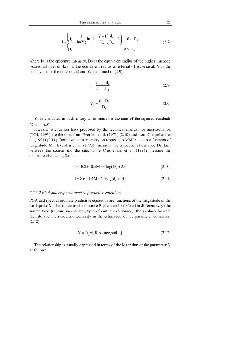
Σ(Iest – Iobs)2. Intensity attenuation laws proposed by the technical manual for microzonation
(TC4, 1993) are the ones from Everden et al. (1973) (2.10) and from Crespellani et al. (1991) (2.11). Both evaluates intensity on respects to MMI scale as a function of magnitude M; Everden et al. (1973) measure the hypocentral distance Dh [km] between the source and the site, while Crespellani et al. (1991) measure the epicentre distance de [km].
hI 10.8 10.5M 6log(D 25)= + - + (2.10) eI 8.6 1.4M 6.4 log(d 14)= + - + (2.11)
2.2.3.2 PGA and response spectra predictive equations
PGA and spectral ordinate predictive equations are functions of the magnitude of the earthquake M, the source-to-site distance R (that can be defined in different way) the source type (rupture mechanism, type of earthquake source), the geology beneath the site and the random uncertainty in the estimation of the parameter of interest (2.12)
( )Y f M, R,source,soil,= ε (2.12)
The relationship is usually expressed in terms of the logarithm of the parameter Y as follow:

24 Chapter 2
4C 2 2 2 21 2 3 5 0 6 0ln Y C C M C M C ln R h C R h= + + + + + + (2.13)
f (source) f (soil)+ + + εσ where C1 is a term that reflects the unit of Y, the terms including C2, C3 and C4 express the exponential relation between the magnitude and the energy released by the earthquake, the term with C5 is due to the geometric spreading of the energy and C6 represents the anelastic attenuation of the energy due to absorption or dissipation.
When using any predictive relationship, it is very important to know how the parameters M and R are defined and their range of validity. A peak ground acceleration predictive equation based exclusively on Italian earthquake recordings (190 horizontal acceleration components) is the one proposed by Sabetta and Pugliese (1996), referred in the following as SP96:
2 2s Ilog A 0.306M log D 5.8 0.169S 1.56 0.17= − + + − ± (2.14)
where Ms is the surface Magnitude 4.6≤ MS ≤6.8, D[km] is the closest distance to surface projection of fault rupture 0≤ D ≤100 and SI is a coefficient for the site geology SI=0 at stiff and deep soil sites and SI=1 at shallow soil sites, ± 0.17 is the standard deviation of the logarithm of the amplitude A, which amounts to a factor 1.5 on a normal scale.
Ambraseys et al. (1996) provide an acceleration spectral value predictive equation, referred in the following as AMB96. This predictive equation is recommended for the European areas as an important part of its dataset consist of earthquakes occurred in Europe and in adjacent regions. It can be employed for different seismicity levels and seismotectonic settings and it makes no distinction among types of source mechanism.
In addition, it uses a simplified ground classification and covers large ranges in distance (up to 200 Km) and of magnitude (4.0≤ MS ≤7.5). The simplified ground classification corresponds to 4 ground classes (from rock to very soft soil) almost coincident with the Eurocode 8 soil classification (CEN 2003).
( ) ' 2 2a 1 2 4 10 0 A A S Slog S C C M C log r h C S C S P= + + + + + +σ (2.15)
where Sa = Sa(T) is the response spectral acceleration at period T[s], (in [g] for T = 0 or [m/s2], C1’, C2, C4, CA, CS, h0 are numerical coefficients, function of the period T, MS is the surface wave magnitude, SA, SS are coefficients for site geology ( SA=SS=0 for rock, SA=1, SS=0 for stiff soil, SA=0, SS=1 for soft soil), r is the shortest distance between the surface projection of the source and the site [Km], P is a coefficient that takes a value P=0 for the 50–percentile and P=1 for the 84–percentile of the prediction.

The seismic risk analysis 25
All these coefficients are provided as a function of the structural period. Table 2.10 shows AMB96 coefficients values for T=0, to be employed for PGA prediction.
T C1' C2 h0 C4 Ca Cs σ ln(10σ)0 -1.48 0.266 3.5 -0.922 0.117 0.124 0.25 0.576
Table 2.10 Numerical coefficients of AMB96 for T = 0 structural period.
2.2.4 Geothecnical zonation and local site effects
It is well established that local site conditions and, to a more limited extend, irregular surface topography can substantially influence the amplitude, the frequency content and the duration of a strong ground motion and consequently can exert a crucial influence on the severity of the damage caused by the earthquake. Whichever approach to hazard estimation is used the influence of site conditions needs to be incorporate.
2.2.4.1 Geothecnical zonation: data to be collected and levels of analysis
A scenario study should aim at producing aerial estimation of damage, and not at predicting the structural response at a specific site. When the aim is a geothecnical zonation to be employed for vulnerability assessment and seismic risk purposes, the representation of the ground conditions, need not to be more detailed than that requested by state of art seismic code and in many cases could actually be simpler
Simplified approaches on respects to the ones normally employed for predicting the ground and the structural response at specific sites can be implemented. The guidelines for performing geothecnical zonation prepared by the technical committee for “Earthquke Geothecnical Engineering” TC4 (1993) describe three grades of approaches to zonation depending on the variation in quantity and quality of the available data. The application of this TC4-Manual for Zonation on Seismic Geothecnical Hazards to Italian regions has shown to provide reliable results (Crespellani et al., 1997).
The handbook for earthquake ground motion scenarios, prepared in the framework of the Risk–UE project (Faccioli and Pessina, 2003), distinguishes between two different levels of approaches depending on the level of knowledge achieved and on the scope of the scenario study. In particular according to a I-level zonation is obtained by the interpretation of the near-surface formations of the geological map in terms of approximate geotechnical units, using available geotechnical parameters, or some seismic response measure. While a II-level approach needs that as much data as possible on the subsoil are collected from public and private sources. Useful data are soil borings, water wells, field geophysical investigations, geotechnical laboratory tests and geotechnical borings, especially those reaching formations that can be regarded as “seismic bedrock”. The collected material has to be careful selected, assembled and processed according to

26 Chapter 2
different steps that allow drawing VS30 contours throughout the urban area.
∑=
=
Ni i
iS
VhV
,1
3030 (2.16)
Both the approximate geotechnical units obtained from a I level approach and the
VS30 contours resulting from the II level approach can be arranged by ground classes following EC8 classification (Table 2.11).
Ground class Description of stratigraphic profile VS30
(m/s) NSPT (bl/30cm)
CU (kPa)
A Rock or other rock-like geological formation, including at most 5 m of weaker material at the surface > 800 - -
B Deposits of very dense sand, gravel, or very stiff clay, at
least several tens of m in thickness, characterised by a gradual increase of mechanical properties with depth
360 - 800 > 50 > 250
C Deep deposits of dense or medium – dense sand, gravel
or stiff clay with thickness from several tens to many hundreds of m
180 – 360 15 - 50 70– 250
D Deposits of loose-to-medium cohesionless soil (with or
without some soft cohesive layers), or of predominantly soft-to-firm cohesive soil
< 180 < 15 < 70
E
A soil profile consisting of a surface alluvium layer with VS30 values of class C or D and thickness varying between about 5 m and 20 m, underlain by stiffer material with VS30 > 800 m/s
S1
Deposits consisting – or containing a layer at least 10 m thick – of soft clays/silts with high plasticity index (PI > 40) and high water content
<100 - 10 – 20
S2 Deposits of liquefiable soils, of sensitive clays, or any
other soil profile not included in classes A-E or S1
Table 2.11 Classification of ground conditions according to EC8 (CEN 2003).
In other words a zonation in terms of EC8 geothecnical units can be obtained
with a different level of detail leading to a higher reliability of the zonation when a deeper knowledge is achieved.
On respect of such a zonation soil amplification phenomena can be accounted for in a different way depending on the parameter employed for the earthquake size description. With regard to intensity, an increment of 0.5 intensity degree could be applied for medium stiff clays and medium dense cohesionless soils (on respect to stiff soils and rock) according to expert opinions or applying empirical correlations like those shown in Bard (1998). If peak ground acceleration or spectral ordinates

The seismic risk analysis 27
are employed for the hazard description, the availability of a zonation provided in terms of EC8 classes allows to take into account site effects; this is a straightforward operation dealing with attenuation laws accounting for soil conditions (see for instance AMB96) as EC8 classification system is usually consistent with predictive equations soil classification system. Alternatively, the predefined spectral shape proposed by EC8 (2003), can be ascribed to a PGA hazard description, depending on the local soil conditions shown by the zonation map.
The I level approach, according to TC4 (1993), makes reference directly to the site surface geology, judged to be a practical and applicable approach to many areas because of the wide availability of geological map. TC4 quotes empirical correlations between surface geology and seismic intensity increment based on observation after earthquake proposed by different authors. Table 2.12 shows what has been proposed by Medvedev (1962) and Evender and Thomson (1985) for intensity increments; Table 2.13 shows spectral acceleration relative amplification factors proposed by Midorikawa (1978).
Medvedev M.S.K. Evernden and Thomson M.M.
Granites 0 Granitic & metamorphic rocks 0 Limestone, Sandstone, Shale 0.2÷1.3 Paleozoic Rock 0.4 Gypsum, Marl 0.6÷1.4 Early Mesozoic rocks 0.8 Coarse-material ground 1÷1.6 Cretaceous to Eocene rocks 1.2 Sandy Ground 1.2÷1.8 Undivided Tertiary rocks 1.3 Clayey Ground 1.2÷2.1 Oligocene to middle pliocene rocks 1.5 Fill 2.3÷3 Pliocene-Pleistocene rocks 2 Moist ground (gravel, sand, clay) 1.7÷2.8 Tertiary volcanic rocks 0.3 Moist fill and soil ground 3.3÷3.9 Quaternary volcanic rocks 0.3
Alluvium (water table<30ft) 3 Alluvium (30ft<water table<100ft) 2 Alluvium (100ft<water table) 1.5
Table 2.12 Intensity increments for geology units.
Midorikawa (1987) Relative amplification factorHolocene 3.0 Pleistocene 2.1 Quaternary volcanic rocks 1.6 Miocene 1.5 Pre-Tertiary 1.0
Table 2.13 Relative site amplification for geology units.
An approach widely used for geothecnical zonation is the method proposed by
Nakamura (1989), by which the site response can be determined evaluating the Fourier spectral ratio of horizontal versus vertical component (H/V spectral ratio) of

28 Chapter 2
microtremors acquired at the same site. Instrumental surveys of background seismic noise on a grid of observation points,
and identification of the frequencies of the dominant peak in the spectral ratios of horizontal to vertical motion, does not lead to geotechnical zonation maps but, more directly, to maps of a response parameter (dominant frequency of ground motion) controlling the shape of the elastic response spectrum. Reliable results are provided when a large impedance contrast between the sediments and the bedrock exists.
Since it can be efficiently carried out, Nakamura’s method can be applied side-by-side with the geotechnical zonation, and later used as a validation tool on predicted ground motion maps.
2.2.4.2 Amplification effects in hazard analysis
Topographic amplifications denote a physical phenomena arising from the propagation of seismic waves in geometrically irregular configurations at the earth surface like canyons, ridges, hilltops. Surface irregularities cause a localized increase in the ground motion amplitude a focusing (defocusing) phenomenon due to the incidence of the waves on a locally convex (concave) surface profile. An additional dynamic phenomenon (resonant motion) affecting the entire profile could be generated if the ways, incident the base, meets certain requirement.
Different effects caused by different geometric and different wave field have been estimated from the exact solutions of idealized problems (Faccioli 1991) leading to amplification factors evaluated as a function of the vertex angle of the wedge.
As very few instrumental data documenting the response of topographic relief exist (Jibson 1987, Paolucci et al. 1999), the evidence of topographic amplification has been explored also starting from historical earthquake. On the basis of the careful analysis of the 1887 Western Liguria Earthquake Faccioli et al. (2002) have established that within an epicenter distance of few tens of km, amplification on markedly irregular topography (i.e. hilltop, crests and severely sloping ground) can account for one (∆I = 1), exceptionally one and a half (∆I = 1.5) or more intensity degrees with respect to the average. Thus, according to Margottini I-PGA correlation (2.3), corresponds to an amplification factor fPGA=1,5 fPGA=2 in the maximum ground acceleration. The results of highly accurate numerical 3D and 2D simulations of the earthquake response of 4 real steep topographic configurations (Paolucci et al., 2002) provide a confirmation of these values.
EC8 3D 2D SH 2D SV Isolated Cliff 1.2 1.3 1.22 1.22 Ridge crest width << base width average slope angle>30° 1.4 1.58 1.18 1.32
Ridge crest width << base width average slope angle<30° 1.2 1.25 1.09 1.28
Table 2.14 Topographic amplification factors from Paolucci (2002).

The seismic risk analysis 29
According to the numerical simulations indeed, topographic amplification factors range between fPGA=1.25 and fPGA=1.75 with an average value of fPGA=1.47.
The topographic amplification factors proposed by EC8, depending on the geometry of the irregularity (Part5 Informative Annex A of EN 1998-5:200X) belongs to the same range values fPGA= 1.2 ÷1.4.
2.2.5. Deterministic and Probabilistic Seismic Hazard Analysis
2.2.5.1 Deterministic Seismic Hazard Analysis
The deterministic scenario postulates the occurrence of an earthquake of specified size at a specified location. Four very simple steps are involved in such an assessment. The first step is the identification of the location and of the characteristics of significant earthquake sources that might affect the studied region: these may be geological faults, where these are clearly mapped or otherwise areas where earthquakes have occurred in the past and for which direct correlations with individual faults is not possible. For each source, an earthquake scenario is then defined, fixing both the magnitude of the earthquake and its distance from the site. With regard to the magnitude to be assigned, reference can be made, for instance, to the maximum historical event from that source (MPE-Maximum Probable Earthquake), or to the maximum earthquake compatible under the known tectonic framework (MCE-Maximum Credible Earthquake) (Kramer, 1996). With regard to the location, the shortest distance from the source to the studied region is generally assumed in order to represent the most unfavourable situation. The third step is the selection of an attenuation relation enabling to estimate the ground shaking within the zone of interest. More than one earthquake scenario may be adopted performing a seismic risk analysis: depending on the purpose of the study it would be necessary to assess the consequences both of a destructive event and of a less severe, but damaging, one.
An alternative approach for a deterministic scenario is to directly make reference to local macroseimic intensities, or to instrumentally measured parameters, generated by a damaging, real earthquake of the past.
2.2.5.2 Probabilistic Seismic Hazard Analysis
Probabilistic Seismic Hazard Analysis (PSHA) has been established since the late 1960es (Cornell, 1968), and has became the most widely used approach to the problem of determining the characteristic of strong ground motion for engineering design. The original formulation has been modified by McGuire (1976) including the influence of the uncertainties in the strong-motion prediction equation. Several modifications and change have been proposed since, but the fundamental mechanism of the calculations remains the same.
The essence of PSHA is the identification of all possible earthquakes that could affect a site, including all feasible combination of magnitude and distance and the

30 Chapter 2
characterisation of the occurrence frequency of different size earthquake through a recurrence relationship.
As for DSHA four are the basic steps. The first step, as in DSHA, is the definition of the source zone, either as line, for clearly mapped faults, or else as general areas. The two fundamental features of the Cornell-McGuire method are the spatially uniform activity for the identified seismogenetic sources and the assumpion of a poisson process to represent the seismicity. The second step is to characterise the seismicity activity in each source in terms of a magnitude-frequency relationship (2.17), truncated at an upper limit referred as Mmax. The value of Mmax can be determined from the leght of known faults within the source and using empirical relationship such as those of Well & Coppersmith (1994). Alternatively Mmax can be estimated by adding an appropriate increment to the magnitude of the largest historical earthquake to have occurred in the zone: the longer and more complete the earthquake record, the smaller the increment.
( )log N a bM= − (2.17)
where N is the annual frequency for the magnitude M and a and b are the
parameters determined by the regression analysis. Attenuation equations are then employed to calculate the ground motion
parameters that would result at the site due to each of these earthquakes and hence the rate at which the different levels of ground motion occur at site is calculated. The last step consist of integration over the whole range of magnitudes and distances considered to obtain, probabilistic hazard values in the form of a distribution, or of exceedence rates, for ground motion parameter of interest.
The probability of exceedance q, is the probability that at least one event occurs in a specified period that exceeds a specified threshold. If P(x) is the probability of x favourable events then the probability of exceedance is defined by:
q 1 P(0)= − (2.18)
The probability of x earthquake of magnitude M or greater during a period of time L is evaluated according to the assumed Poisson Process.
( )x LNLN e
P(x)x!
−
= (2.19)
The probability of exceedance of an earthquake with magnitude M during a
period of time L is therefore given by:
LNq 1 e−= − (2.20)

The seismic risk analysis 31
To better understand the steps according to which a PHSA analysis is performed, the procedure can be considered with regard to a single point seismic source. Wanting to evaluate the probability of exceedance of a certain PGA level in a certain area because of this source, the first step is to asses the magnitude required to produce this level of acceleration at the source-site distance. This is possible making explicit M from an assumed predictive correlation (2.12).
The annual frequency of earthquakes at the source characterized by this magnitude M can be therefore evaluated from the recurrence relationship (2.17):
( ) 0bMa
0N PGA 10 10−= (2.21)
Substituting the value of N(PGA0) so determined in (2.17), the corresponding probability q0 of exceed PGA0 value can be found. Repeating this procedure for different levels of PGA, hazard curves (PGA-q) can be drawn.
PHSA analysis results extending the procedure described for the single point seismic source to each of the general area or line sources identified by considering each source to be made up of a collection of points and integrating the contributions from all of these. Some computational tools implementing Cornell’s method for PSHA are available since quite a few years, i.e. SEISRISKIII (Bender and Perkins 1987) or CRISIS99 developed by M. Ordaz (Ordaz et al. 1989).
2.2.5.3 Probabilistic or deterministic hazard analysis
Whenever the study of risk is conducted in probabilistic terms, the loss and the economic consequences will be expressed probabilistically as well: this approach represents that which is called a risk analysis. Instead, in the case in which the seismicity is studied on a deterministic basis, a scenario analysis is carried out.
The choice between risk analysis and scenario analysis depends on the aims of the study. In the case of a study of the territory for preventive purposes, a risk analysis is preferable in that it brings together the effects of all the potential seismic sources of the area and supplies a comparable evaluation between all the different communities interested by the study. Instead, to analyze the aspects of management of the emergency linked with the Civil Defense, a scenario analysis is the most significant, in that it reproduces a realistic distribution of the effects on the territory, a fact that allows elaboration of strategies for the post-earthquake.
However it has been well recognized that, there is not a mutually exclusive dichotomy between DSHA and PSHA, opening up the possibility of exploring combined methods (Bommer 2002). The main differences between PSHA and DSHA are that PSHA has unit of time (so the chance to characterize the rate at which earthquakes and particular levels of ground motion occurs) and DSHA not (but it does not mean that time and probabilities cannot be attached to determinist scenarios). The second difference is the way in which the hazard from different sources of seismicity is treated. DSHA treats seismogenetic sources separately while

32 Chapter 2
PSHA combines the contributions from all relevant sources into a single rate for each level of a particular ground motion parameter. A combined solution explored in loss estimation studies is to model the hazard as a series of earthquake scenarios, to each of which an average rate from the recurrence relationship is assigned.
2.2.5.4 Modelling the uncertainty in the hazard analysis
A wide exploration of the uncertainties affecting the ground motion prediction is contained in Restrepo-Velez and Bommer (2003) where two different types of ground motion uncertainty sources are distinguished: aleatory and epistemic.
The aleatory uncertainty is related to the unpredictability of the earthquake generating process. In the framework of a seismic hazard assessment it is represented and summarized by the standard deviation of the probability density function of the predictive equation (making reference to (2.13) is the standard deviation of lnY at the magnitude and distance of interest). The predictive equation scatter must be incorporated into seismic hazard assessment and its influence can be very meaningful; as a matter of fact very significant influence on the results of PSHA as well as on DSHA have been observed if 84-percentile values are considered instead of mean value.
The epistemic uncertainty is due to the lack of knowledge as for instance about the definition of the seismic source geometric features (rupture length, strike, dip angle) or about the activity of the sources, as well as about the recurrence model or the selection of the most suitable predictive equation. They cannot be measured in the same explicit function as aleatory uncertainties as they are generally connected to factors involving subjective decision making. Therefore, epistemic uncertainties are represented in the hazard assessment by means of a logic-tree formulation.
A logic tree is used in the following way. Each end branch represent a complete set of assumptions: a PSHA or a DSHA is conducted for each end branch and a seismic hazard curve is derived. To each seismic hazard curve a weight is assigned equal to the product of the probabilities on the branches leading to its corresponding end branch. Thus there is a family of hazard curves with weight that sum to unity. From this family, a mean hazard curve can be calculated as well as fractile of annual frequency of exceedance.
It is important to bear in mind that the logic tree formulation (considered to be a rational method for dealing with uncertainty in PSHA) does not actually reduce the uncertainty at all. Furthermore the approach addresses the problem of uncertainty associated with subjective decision by introducing a series of subjectively determined weights and then subjecting these to statistical analysis.
Anyway, establishing a logic-tree without the weights has been proved to be useful both for PSHA and for DSHA approaches in order to dispose of an ordered framework for carrying out a sensitivity analysis.

The seismic risk analysis 33
2.3 VULNERABILITY ANALYSIS
2.3.1 Brief state of the art for seismic vulnerability methods
The seismic vulnerability for a built system is defined as its susceptibility to suffer a certain damage level if subjected to an earthquake. In compliance with this definition, the aim of a seismic vulnerability method is to provide a measure of the propensity for a building or of a set of building to be damaged if hit by an earthquake. In operative terms and on respects to the definitions of seismic risk provided in (1.1), a vulnerability method must correlate the seismic hazard evaluation to the physical damage suffered by the built system depending on the structural, geometric, technological characteristics able to affect the seismic building behavior.
Several methods for the vulnerability assessment have been developed and proposed in recent years and, consequently, several have been the attempts to provide classification criteria for them (Corsanego and Petrini, 1994; Dolce et al. 1994; UNDP/UNIDO, 1985). The analysed classification criteria agree on the distinction between three types of vulnerability approaches when reference is made to the genesis of the methods. Considering how and on the basis of what knowledge the methods have been derived it is possible to recognize:
- observed vulnerability methods (also referred as empirical approach or statistical methods), based on statistical observations of recorded damage data of past events as a function of the felt intensity;
- analytical methods, based on the mechanical calculation of building structural response;
- method based on expert judgment. These approaches are differently characterized by positive features and
limitations so that recent experiences have also considered the possibility of hybrid techniques.
2.3.1.1 Observed vulnerability methods
Observed vulnerability methods are based on statistics of past earthquake damage data. One of the first to have systematically compiled statistics on damage to buildings from experiences after recent earthquakes was Withman (1973). From a survey of damage caused by the San Fernando earthquake of 9 February 1971 damage probability matrix (DPM) were generated for different building types. The general form of such a damage probability matrix is shown in Table 2.15. Each number in the matrix expresses the probability that a building of a certain class will experience a particular level of damage as a result of earthquake intensity.

34 Chapter 2
Intensity of Earthquake DamageGrade
Structural Damage
Non - StructuralDamage V VI VII VIII IX
0 None None … … … … … 1 None Minor … … … … … 2 None Localized … … … … … 3 Not noticeable Widespread … … … … … 4 Minor Substantial … … … … … 5 Substantial Extensive … … … … … 6 Major Nearly Total … … … … … 7 Building Condemned … … … … … 8 Collapse … … … … …
Table 2.15 Format for a Damage Probability Matrix after Whitman (1974).
The format of DPM has become one of the most widely used forms to define the
probable distribution of damage, adapted by several other methods. The GNDT I level approach (Corsanego and Petrini, 1994) is, for instance, a DPM based method, having three classes of vulnerability, from A to C, to each of which a DPM is ascribed. GNDT DPM have been drawn by statistical data processing after Irpinia earthquake (Braga et al., 1982) These data have been subsequently updated and regionalized on the basis of several earthquakes. Differently from DPM proposed by Whitman, GNDT damage probability matrix make reference to MCS intensity rather then to MMI and describe the damage by means of a five damage grade scale.
Another approach based on the statistical processing of data collected after different earthquakes from a range of different countries is the one proposed by Coburn and Spence (1992). Five different damage grades are considered. For each building type, the scatter of the intensity at which each individual structures passes a given damage threshold is assumed to be normally distributed. The damage distribution is expressed graphically by the probability of overcame a certain damage grade given the seismic input in terms of a parameter-less scale of intensity.
Generally speaking, observed damage data are limited and do not concern all the building typologies and all the intensities that it would be necessary to represent in a vulnerability model. For this reason, the probabilistic processing of the observed data, at the root of observational methods, is often supported or completely replaced by other approaches such as mechanical analysis (Kappos et al. 1995, Singhal and Kiremidjian 1996), neural network system (Dong et al., 1988), Fuzzy Set Theory (Sanchez-Silva and Garcia, 2001) expert judgement (ATC13, 1987).
2.3.1.2 Expert based methods
The first systematic attempt to codify the seismic vulnerability of buildings from expert judgement was made by Applied Technology Council (funded by FEMA Federal Emergency Management Agency) and summarized in ATC13 (1987) report. ATC13 essentially derived damage probability matrix for 78 different earthquake

The seismic risk analysis 35
engineering facility classes, 40 of which refer to building, by asking 58 expert, based on their personal knowledge and experience, to estimate expected percentage of damage and loss that would result to a specific structural type subjected to a given intensity. Nevertheless the uncertainty related to the opinion of experts, ATC-13 has become the standard reference for earthquake damage and loss estimation study until the mid 1990’s.
Score assignment procedures, known as inspection or rating methods, can be as well regarded as expert based method. They aim to evaluate the building vulnerability weighting the effects of structural deficiencies, from observed correlations between damage and structural characteristics or from simplified mechanical methods; anyway expert judgement is employed in order to assign scores to the different deficiencies.
A score assignment procedure, referred as ATC21 (1988) rapid visual screening procedure was proposed by Applied Technology Council and sponsored by FEMA in 1998 (FEMA 154). According to this approach a basic structural score (BSH) is assigned depending on the primary structural lateral force resisting system and on the material (12 different building types are distinguished) and depending on the level of seismicity characterizing the analysed area. A final structural score is then obtained adding or subtracting performance modification factors to the BSH, if significant seismic-related deficiencies are recognized. The final structural scores typically range between 0 and 6, whit higher scores corresponding to a better seismic performance. Depending on the final structural scores value, the probability for each building to sustain a major life-threatening structural damage during a major earthquake, is evaluated. ATC21 is a therefore a method for single building vulnerability assessment. From ATC21 a model allowing the estimation of earthquake damage and losses for a large community of building has been subsequently proposed by McCormack and Rad (1997).
A method for vulnerability assessment and damage estimation based on score assignments has been also developed and applied successfully in Italy referred as GNDT II level approach (Benedetti and Petrini 1984). According to this method, a vulnerability index Iv is assigned to each building after a visual inspection aiming to identify the building primary structural system and significant seismic related deficiencies. This method, based on a great amount of damage data corresponding to several seismic zones of Italy, recognizes eleven parameters as the most important in controlling the building damage caused by earthquakes: structural system organization, structural system quality, conventional strength, retaining walls and foundations, floor system, configuration in plant, configuration in elevation, maximum distance between walls, roof type, non structural elements and preservation state. The vulnerability index Iv is obtained combining, by a weighed average, the different scores and the relative weights attributed to these parameters. Iv ranges from 0 to 382.5 but eventually can be normalized from 0 to 100, being 0 the best vulnerability condition and 100 the worst. For a given value of the vulnerability index there is a corresponding curve correlating the damage ratio (ratio

36 Chapter 2
between the cost of repair and the cost of rebuilding) to the seismic demand (described in terms of PGA) by means of a tri-linear fragility curve.
2.3.1.3 Analytical Approaches
In the United States and nowadays also in Europe, the most recent trends in the field of vulnerability evaluation for risk analysis lead to operate with simplified mechanical models, essentially based on the Capacity Spectrum Method (Freeman 1998). One of the most worldwide known is HAZUS (1999) a methodology developed by the Federal Emergency Management Agency specifically for U.S. built environment (HAZard in U.S.), but often applied in other regions (Spence et al. 2003).
The methodology is based on three fundamental concepts: capacity curve, performance point and fragility curve. Capacity curve represent the relation between the lateral load resistance of a given structure and its characteristics lateral displacement (Kircher et al. 1997) and it is typically obtained by means of a static pushover analysis. The capacity curve is then converted to spectral acceleration and roof displacement so that it can be compared with the demand spectrum in order to obtain the performance point. With the aim to asses the damage conditions of a building hit by an earthquake the evaluated performance point is compared with defined damage limit states. 36 model building types are considered by the methodology. For each one HAZUS manual provides specific capacity curves as well as the parameters defining fragility curves that allow representing the probability of reaching or exceeding a specific damage limit state for a given ground motion demand.
Other proposals for simplified analytical approaches make reference to displacement based procedure rather then to force based procedure. This is the case of the method developed by Calvi (1999) based on the assessment of the displacement capacity of a building corresponding to several limit states and of the displacement demand resulting from a displacement spectrum. Building typologies are identified on the basis of the period of construction, the number of stories and the construction material (reinforced concrete or masonry). Four limit states are considered taking into account structural and non structural damage. For each type of building structure and for each limit state a structural model is defined in terms of secant stiffness corresponding to the maximum displacement of the limit state considered, from which the equivalent period of vibration is obtained, and a displacement demand reduction factor depending on the structure energy dissipation. The method allows evaluating the probability of occurrence of a certain limit state for a given displacement response spectrum.
Apart from the methods above shortly described a detailed treatment of analytical methods is provided by Miranda and Akkar (2002) and ATC (2002).
Methods that make use of the so-called collapse multipliers, in order to identify the most probable collapse mechanism, have to be as well numbered among the analytical methods. The identification of collapse mechanism is indeed defined on

The seismic risk analysis 37
the basis of mechanical considerations and the collapse multiplier is evaluated by means of a static equivalent procedure. A collapse multiplier approach is the VULNUS method developed at the University of Padova (Beranardini et al. 1999) for the vulnerability assessment of a single building or of a group of buildings, based on the evaluation of geometrical and mechanical characteristics (and other important factors controlling the response of the structure) measured through qualitative judgement and consequently handled under the fuzzy set theory. Another method based on collapse multipliers is the “Failure mechanism identification and vulnerability evaluation method” (FaMIVE), one of the most recent and complete (D’Ayala and Speranza, 2003) for the vulnerability of buildings belonging to historical centres. It employs a predefined set of rules in the definition of the most probable collapse mechanism, either in-plane or out-of-plane.
The output of both VULNUS and FaMIVE methods is the activation threshold of the collapse mechanism; in order to obtain damage scenarios, a safety criterion may be established comparing the collapse multiplier values with the seismic demand amount resulting from a hazard analysis.
2.3.1.4 Critical review of vulnerability methods on respects to seismic risk analysis requirements
As a seismic risk analysis is an integrated approach, the choice of a suitable method for the vulnerability assessment strictly depends, and strongly influences, all the other steps defining the analysis (hazard description, exposure characterisation and damage evaluation).
With regard to the exposure characterisation the choice of the vulnerability method varies according to how in detail the built system can be known and characterized. As a matter of fact, depending on the amount and the quality of the available data and the extension and importance of the analysed area, the vulnerability method has to make reference to a single building, a building typology, a building category or a vulnerability class.
Considering the hazard analysis, the seismic input could be provided in terms of a physical parameter or in terms of a macroseismic size. A vulnerability method usually refers to one of the two, depending on its genesis (observed, expert based or analytical approach).
Finally the adverse effect of the seismic event could be expressed by the vulnerability method, in terms of the physical state of the built system or directly in terms of losses. Damage Probability Matrices, Vulnerability Curves and Vulnerability Scores allow obtaining a direct evaluation in terms of physical damage while Fragility Curves can possibly provide loss results.
For each of the vulnerability methods mentioned in the paragraphs above, Table 2.16 shows how the element at risk are classified, how the seismic input and the output are represented and the tool employed for the building vulnerability description. From Table 2.16 it can be observed that, for the seismic input representation, observational methods and expert based methods make reference to

38 Chapter 2
macroseismic intensity; this is the case of ATC13 and also of GNDT II level that only apparently is based on PGA (Giovinazzi and Lagomarsino, 2001). On the other hand it can be observed that mechanical method refers to physical parameters like PGA or response spectra.
Building System
Description Hazard Damage Vulnerability Description
GNDT - I Level Vulnerability Classes
MCS Intensity Damage DPM
Mac
rose
ism
ic
Coburn and Spence (1992)
Building Typologies
PSI scale Damage Fragility Curves
HAZUS (1999) Building Typologies ADRS Damage Capacity Curve
Calvi (1999) Building Categories DS Damage Structural Parameters
VULNUS Single Building/ Set of Buildings PGA Safety
Criterion Collapse Multiplier Ana
lytic
al
FAMIVE Single Building PGA Safety Criterion Collapse Multiplier
ATC13 Building Typologies
MMI Intensity Losses Fragility Curves
ATC21 Single Building PGA Safety Criterion Vulnerability Score
Expe
rt
GNDT – II Level Single Building Losses Vulnerability Score/ Fragility Curves
where ADRS = Acceleration Displacement Response Spectra and DS = Displacement Spectra.
Table 2.16 Building system, hazard, damage and vulnerability description for different vulnerability methods.
The output representation is mostly in terms of physical damage and anyway for
the few cases providing directly economic losses it must be remembered that these estimations have been obtained correlating the physical damage to losses and that, wanting to evaluate others consequences caused by the building damage, it is necessary to come back to the physical damage.
With regard to the building system characterisation and description, reference is specifically made to single buildings or to class of buildings (a part from VULNUS that can be indifferently applied for single and class of building). Thus means that performing a study for different scale of analysis (local or territorial scale) it is not possible to operate with the same vulnerability method. Moreover, with regard to methods aiming to the assessment of single building vulnerability an observed limitation is that they strictly refer to predefined knowledge forms requiring a specific survey.
The seismic risk analysis 39
2.3.2 Definitions for macroseimic methods and mechanical-based methods
In the framework of this Ph.D thesis, the proposal for original vulnerability methods has taken into account the multitude of experiences carried out during recent years in the field of vulnerability assessment (shortly summarised in the previous paragraph) making the most of their positive features and trying to overcome their problematic aspects.
In particular, with regard to observed damage approaches it has been observed that because of the differences in the way data have been collected and processed and because of the difference in the seismic input and damage description, a unique procedure for these methods is not yet recognized. With regard to mechanical methods, it has been observed that nevertheless they are quite well codified and that they provide reliable results for built-up area characterized by consolidated seismic design codes, their application on traditional non-designed masonry constructions is not yet obvious.
Thus, in order to have a reference universally recognized throughout European regions, an observational method, referred to as the Macroseismic method, has been derived from EMS-98 macroseismic scale definitions to be employed when the seismic hazard is described in term of macroseismic intensity.
On the other hand, a Mechanical method has been developed to be employed when the hazard is provided in terms of PGA or response spectra; capacity curves for the representation of the building behaviours in the framework of the proposed mechanical method have been evaluated by simplified mechanical approaches. In particular, for non-designed masonry building typologies, a simplified mechanical approach has been developed taking into account geometrical features, mechanical parameters, prevalent collapse mode, and dynamic characteristics of the buildings, while, for designed reinforced concrete buildings, capacity curves have been derived from code prescriptions.
In the following a glossary of the main terms and definitions employed by the Macroseismic and by the Mechanical models is provided. These definitions are the ones to which reference is made in Charter 3 and Charter 4 where the proposed Macroseimic and Mechanical methods are presented.
2.3.2.1 Glossary for Macroseismic Methods
Damage grade
As Macroseismic methods are directly or indirectly derived from the observed damage, the damage scale they make reference corresponds to the one employed by macroseismic scale. In modern macroseismic scales the damage is represented in a discrete form through five damage grades DGk (k=1÷5). Table 2.17 shows EMS-98 (Grunthal 1998) five damage grade scale assumed for the macroseimic method.

40 Chapter 2
Damage Grade (DG) DG1 DG2 DG3 DG4 DG5 Structural Damage Slight Moderate Heavy Very heavy Destruction
Table 2.17 Definition of the damage grades DGk according to the Macroseismic Method.
Mean Damage Grade
If a set of buildings is considered, an earthquake of a given intensity should cause a different damage grade in each one of them, due to the specific seismic behaviour. By considering the histogram of the damage grades occurred to the set of buildings, it is possible to define as representative parameter the mean damage grade µD:
5
D kk 0p k=
=µ ∑ D0 5< µ < (2.22)
where pk is the probability of having damage of grade k, in the set of buildings. It is worth noting that the mean damage grade µD is a continuous parameter, unlike the damage grades, which represents the distribution of damage to the building set.
Damage Factor
The damage can also be measured in economic terms through a parameter, the damage factor (DF), which is defined as the ratio between repair cost and reconstruction cost (the latter corresponds to the value of the building):
Repair CostMDR DFBuilding Value
= = (2.23)
Damage Probability Matrix (DPM)
A damage probability matrix (DPM) is a matrix that contains the seismic response of a set of buildings, by expressing the statistical distribution of damage grades for the different macroseismic intensities. In other words DPM express in a discrete form the conditional probability P[DGk | T, I] to obtain a damage grade DGk due to an earthquake of severity (I) for a defined typological class T (Table 2.15).
Vulnerability Index
The vulnerability index is a continuous parameter that quantifies the disposition of a building (or of a set of buildings) to be damaged by an earthquake; in other terms, the vulnerability index is a score that can be assigned to a building by means of available information on the typology and other structural and constructive characteristics.

The seismic risk analysis 41
Macroseismic Fragility Curves
The fragility curves provide the probability of being in or exceeding, for a given set of buildings, a given damage grade or a certain consequence (damage grades, economic losses, collapsed buildings, unfit for use buildings, dead people, homeless), as a function of the macroseismic intensity.
2.3.2.2 Glossary for mechanical-based methods
Demand Spectrum
The Demand Spectrum, also called ADRS - Acceleration Displacement Response Spectrum, is the representation of earthquake response spectra of acceleration and displacement into a unique diagram. Each point of the diagram, in spectral coordinates, corresponds to a different period of vibration.
Capacity Spectrum
The Capacity Spectrum also called capacity curve, represents the inelastic capacity of the structure obtained by a pushover analysis. In order to obtain a capacity spectrum from the results of a pushover analysis it is necessary to define a s.d.o.f. equivalent structure and to perform a point-by-point conversion to the first mode spectral coordinates so that each point of the pushover curve is converted to a Sa, Sd point.
Performance Point
The Performance Point represents the demand of strength and displacement, obtained by intersecting the capacity spectrum with the demand spectrum.
Damage State
Damage states DSk are defined by opportune ranges of the spectral displacement value (performance point abscissa). Typically 4 damage states DSk (k=1÷4) are considered, beyond the no damage condition.
Damage State (DSk) DS1 DS2 DS3 DS4 Structural Damage Slight Moderate Extensive Complete
Table 2.18 Definition of the damage states DSk according to the Mechanical Method.
Fragility Curves
The Fragility Curves provide the probability of being in or exceeding a given damage state, as a function of the demanded spectral displacement (to be considered as an estimation of the mean value), obtained with the performance point.

42 Chapter 2
2.4 ESTIMATION OF SEISMIC LOSSES AND CONSEQUENCES
Structural and non structural damages are the root cause of many of the other losses expected after an earthquake. Direct economic losses, consequences to buildings and their content, consequences to inhabitants can be estimated after physical damage has been determined. To this aim statistical correlations, translating structural and non structural damage into percentage of losses are proposed by different authors and in the framework of different seismic risk analysis methods. These correlations seems to be different, however it has been found that they can be reported in terms of a same formulation.
As a matter of fact the occurrence probability of particular consequences pC
because of an earthquake can be obtained combining the probability of having a certain damage grade pk by weight factors wC,k.
C C,k kk
p w p= ∑ (2.24)
As loss and consequence correlations are associated both to mechanical and
macroseismic approaches, in order to provide a homogeneous state of the art and to make a comparison between the results supplied by these different proposals it is necessary, first of all, to establish a unique physical damage representation.
With respect to the 5 damage grade scale (DGk k=1÷5) considered by observational methods (related to a qualitative damage observation during the post-earthquake survey), mechanical approaches refer to a 4 damage limit state scale (DSk k=1÷4), usually related to performance levels. A perfect correspondence between the first 3 can be considered, thus last two damage grades, corresponding to the fourth damage state, can hardly be distinguished in a mechanical model: in fact it is clear that, while watching it is easy to distinguish what is collapsed from what is heavily damaged (but still standing), the same distinction is not possible on a curve, when the structure has lost its static resources.
D1 D2 D3 D4 D5 DG Slight (DG1) Moderate (DG2) Heavy (DG3) Very heavy (DG4) Destruction (DG5)DS Slight (DS1) Moderate (DS2) Extensive (DS3) Complete (DS4)
Table 2.19 Correspondence between Damage State DSk and Damage Grade DGk.
In the framework of this Ph.D thesis, reference is made to a discrete five damage
scale Dk (k=1÷5) coincident to the damage scale adopted by EMS-98 macroseismic scale (Grunthal 1998).
Consequently, loss and consequence fragility curves can be obtained as follow:

The seismic risk analysis 43
( ) [ ]C C,k C,k 1 kk
w w DP P−= −∑ (2.25)
2.4.1 Collapsed and uninhabitable buildings
Collapsed buildings are the ones suffering damage D5 (Table 2.19). Uninhabitable dwelling are for sure the units located in buildings that are in a complete damage state in addition to a percentage of the ones located in building suffering minor damage.
HAZUS (1999) proposal and an Italian proposal (Bramerini 1995), shortly referred as SSN, are considered in the following. Both evaluate the percentage of uninhabitable dwelling pUd starting from damage D3 but attributing different rates (weight factor wUd,k) to each damage grade:
Ud Ud,3 3 Ud,4 4 Ud,5 5p w p w p w p= + + (2.26)
where p3, p4, p5, are the probability of occurrence for damage D3, D4 and D5 and wUd,3 w Ud,4 w Ud,5 are weight factors of this probability considered to provide the percentage of uninhabitable dwelling for each damage grade.
The weighted factors proposed by the two approaches are shown in Table 2.20. In particular HAZUS distinguishes between single and multi-family structures (quoted respectively as SFD and MFD) with the aim of including in the computation also the number of damaged units that are perceived to be uninhabitable by their occupants. For this reason the weight factors are higher in the case of multi-family structures as it is considered that people living in single-family homes are much more likely to tolerate damage in their own home on respect to the renters living in multi-family structures.
k wUd,k HAZUS (SFD) HAZUS (MFD) SSN (All)D 3 wUd,3 0 0.9 0.4 D 4 wUd,4 1 1 1 D 5 w Ud,5 1 1 1
Table 2.20 HAZUS weighted factors wUd,k for uninhabitable dwelling.
It is worth noting that HAZUS does not provide originally the weight factor for
collapse D5. According to what previously observed about the correspondence between the adopted damage scale and mechanical method damage limit states (Table 2.19) the same value provided by HAZUS for D4 has been assumed for D5 (w
Ud,4 =w Ud,5 ). Once the percentage of uninhabitable dwelling pUd has been evaluated, the total
number of uninhabitable units NUd due to structural damage is obtained multiplying this probability for the number of dwelling unit Nd available from building inventory
44 Chapter 2
data collected in the framework of an exposure analysis:
Ud d UdN N p= (2.27)
If distinction has been done between single-and multi family dwelling units formula (2.27) results in: ( ) ( )Ud SFd MFdUd SF Ud MFN N p N p= + (2.28)
where NSFd and NMFd are respectively the number of single and multi family
dwelling units and pUd(SF), pUd(MF) the probability of having these dwelling uninhabitable, evaluated according to formula (2.26) and Table 2.20 weight factors. The uninhabitable household estimates can be then combined with demographic data to quantify number and composition of population requiring short term shelter.
2.4.2 Casualties
Earthquake casualty modelling is fundamental not only for emergency response management and for mitigation strategy planning, but also for health preparedness planning.
Nevertheless the world’s seismic literature is replete with accounts of devastation caused by earthquakes (an earthquake kills more than 5000 people on average every 900 days) there is the awareness that a lot of work has to be done for a more specific estimation of earthquake casualty.
According to Jones et al. (1993) serious doubts exist as to the validity of the existing causality estimation functions that are mostly based on engineering functions with little input from medicine or epidemiological studies. In the same way HAZUS (1999) clearly identifies the deficit of data that exists in this field of casualty evaluation and states that this limits the reliability of the estimates. Input from medicine or epidemiological studies should be included in the casualty modelling. These studies highlight that several parameters further than building characteristics have shown to affect the number of casualty after an earthquake. Definitely an important influence is provided by the occupant characteristics (age, sex, social condition) and their likely actions in earthquake (Durkin and Thiel, 1993); Peek-Asa et al. (1998) quote that predominant number of casualties in 1994 Northbridge earthquake involved older people: people over 65 accounted for 31.2% of the fatalities and 75.8% of the hospitalised injuries. The performance of non structural elements and building contents have shown to be the major source of minor injuries; moreover the experience of Whittier Narrows (1987), Loma Prietra (1989) and Northridge earthquake (1994) indicates that minor injuries result primarily from being struck by falling objects. Without doubts the availability of rescue and medical facilities treating those affected is a very influential factor in the

The seismic risk analysis 45
casualty number. It has been highlighted that a non negligible number of affected people come from secondary hazards (fire following earthquake, landslides, release of toxic substances).
In the following some method proposed in literature for the casualty estimation are reviewed distinguishing between models that related the death rate to building damage (referred as building specified approaches) and more general approaches that provides estimates independently from building damage (non building specified approaches).
2.4.2.1 Non building specified casualty models
Non building specified approaches develop causality estimates for geographical area or for population density correlating gross mortality ratio with the size of the earthquake. A proposal made in the framework of Risk-Ue Project WP7-Report (Vacareanu et al., 2004) relates the number of deaths to the magnitude of the earthquake. Representing human losses from several earthquakes occurred in different country as a function of the earthquake magnitude (Figure 2.4) a correlation has been derived:
1.5MD ce= (2.29) where D is the number of deaths, M is the magnitude of the earthquake and c is a coefficient assuming different values for lower, medium and upper bounds (respectively c = 0.002, c = 0.06, c = 0.4).
Major earthquakes in 20 th century
USA, Northridge, 1994USA, Loma Prieta, 1989
Japan, Kobe, 1995Italy, 1980
Turkey, Kocaeli, 1999Nicaragua, 1972
Guatemala, 1976
Taiwan, 1999
Romania, 1977Colombia, 1999El Salvador, 1986
Mexico, 1985
Iran, 1990
Armenia, 1988
Philippines, 1990Skopje, 1963
Montenegro, 1979
1
10
100
1,000
10,000
100,000
5.5 6 6.5 7 7.5 8 8
Magnitude, M
Dea
ths,
D
D =0.06e1.5M
Figure 2.4 Human losses represented as a function of earthquake magnitude. A further example of non building specified approach is the very crude prediction
of casualty rates based on the population derived by Peek-Asa et al. (2000)

46 Chapter 2
depending on the Intensity level (from the 1994 Northridge earthquake).
MMI Casualty rate* (per 100000 population)
<VI 0.03 VI 0.16 VII 2.1 VIII 5.1 IX 44
Casualty rate* fatalities and injuries requiring hospitalization
Table 2.21 Casualty rate as a function of MMI (Peek-Asa et al. 2000). It is important to highlight that building specified approach do not take into
account the type of construction, the severity of injury and other factors; for these reasons they are considered non suitable for seismic risk analysis purposes a part from providing a superior and inferior bounds that can be useful in order to verify the reliability of the results obtained by the application of building specified approaches.
The proportions provided between death and non-fatalities injured have to be considered in the same perspective. The total number of non-fatalities injured from earthquake has been found to be 3 to 4 times the number of fatalities (Alexander, 1996), although the ratio varies greatly from earthquake to earthquake. An average ratio from 3:1 to 4:1 could be employed in order to make preliminary estimates. These ratios are representative of serious and moderate injuries (those requiring treatment at hospital) because minor injuries can be very numerous. For example, Shoaf et al. (2001) found that all injuries from 1994 Northridge earthquake (including those that were not treated) numbered in the hundred of thousand, whereas there were only 33 fatalities.
27
6
DOA
Die in hospital
9
129
Hospitalized/Trauma Cases
Hospitalized/Non-Trauma
8,200
16,400
Emergency DepartmentTreat & Release
Out of HospitalTreat & Release
221,400Injured notreatment
InjuryPyramid:
NorthridgeEarthquake
Figure 2.5 Injury Pyramid: Northridge Earthquake.

The seismic risk analysis 47
2.4.2.2 Building specified casualty models
For risk estimates, predictions of casualties must ultimately be based on structural damage. In this way it is possible to take into account not only building characteristics but also the hazard description (resulting from the earthquake magnitude, the attenuation and local site effects) being already included in the resulting physical damage affecting the buildings. Moreover it is possible to take into account the potentiality of the people presence inside the building, making reference to data available from exposure analysis and making hypothesis about the occurrence of the event in a particular hour, day and season.
Similarly to the correlations provided for the estimation of uninhabitable dwelling the correlations provided for the casualty estimation can be lead back in the form of a combination between the probability of certain damage grade pk and some weight factors wC,k.
Tiedmann (1990, 1989) provides approximate Death Rate (DR in percentage of the population) correlations depending on MMI Intensity for different building typologies. Seven typologies of decreasing vulnerability are considered A÷E, A = Irregular masonry (poor), B =Regular masonry (block/brick), C =Reinforced Concrete-RC (pre-1960), D =Reinforced Concrete-RC (1960÷1985), E =Reinforced Concrete-RC (post -1985). The correlations are intended for average soil condition (medium hard alluvium) and moderately irregular buildings; corrections are proposed for particular subsoil quality and for irregular buildings. With regard to the potentiality of people inside the building, the death rate has been estimated for average condition assuming neither rush hour traffic nor seasonal effects and it does not include the causalities to be expected from secondary hazards (fire, tsunami, landslides). According to what previously highlighted, the same author stresses that such correlations should be used with great care because of the general uncertainties afflicting such data and because of the many variables parameters that determine the behaviour of building and hence the number of victims.
Figure 2.6 Death Rate for vulnerability classes depending on MMI Intensity.

48 Chapter 2
ATC13 (1987) provides a building specified casualty model on the basis of expert opinions (calibrated on past-earthquake observations and on previous proposals) making reference to a three level injury severity scale (Minor Injuries, Serious Injuries, Deaths).
Rates in Table 2.22 are intended for masonry and reinforced concrete typologies while for light steel and wood frame constructions the numerators have to be multiplied by a 0.1 factor.
Damage State MDR Minor Injuries Serious Injuries Deaths
Slight 0-1 3/100.000 1/250.000 0.02 Light 1-10 3/10.000 1/25.000 0.04 Moderate 10-30 3/1000 1/2500 0.02 Heavy 30-60 3/100 1/250 Major 60-100 3/10 1/25 Destroyed 100 2/5 2/5
Table 2.22 ATC13 casualty rates.
With regards to the assessment of the number of injuries neither correlations nor
standardised graphs are provided by the previously mentioned approaches, but it is assumed that a plausible ratio of people killed to people injured is about 1÷3 to 1÷6.
Among the building specified casualty approaches, HAZUS (1999), Coburn & Spence (1992), and an Italian proposal (Bernardini 1995), shortly referred as SSN have been considered. All these correlations evaluate casualty rates on respect to a four levels injury severity scale (Table 2.23).
Severity Level Injury Description
S1 Injuries requiring basic medical aid without requiring hospitalization S2 Injuries requiring a greater degree of medical care and hospitalisation,
but not expected to progress to a life threatening status S3 Injuries that pose an immediate life threatening condition if not treated
adequately and expeditiously. The majority of these injuries are the result of structural collapse and subsequent entrapment or impairment of the occupants.
S4 Instantaneously killed or mortally injured
Table 2.23 Four level injury severity scale. Even thought more elaborate scales exist (two common injury scales are the AIS
Abbreviate Injury Scale (Peek-Asa et al., 2000) ratings from 1-9 and the ISS 0-75, (Noji 1989) the classification presented in Table 2.21 is universally recognized in the framework of casualty models for seismic risk analysis purposes as it represents an achievable compromise between the demands of the medical community and the ability of engineering community to provide the required data.

The seismic risk analysis 49
HAZUS proposal considers that a certain casualty rate is provided by each damage state (D1 slight, D2 moderate, D3 extensive, D4 complete and D5 complete with collapse structural damage):
5
Si Si,k kk 1
p w p=
= ∑ (2.30)
where psi is the probability for people involved in an earthquake to suffer a i-
severity (i= 1÷4) pk, is the probability of a damage Dk, (k=1÷5) occurrence and wsi,k
is the weight factor considered for pk probability (Table 2.24). HAZUS manual provides indoor and outdoor casualty rates by building typology
for slight D1, moderate D2, extensive D3, complete D4, complete with collapse D5 structural damage state.
Damage state Dk S1 S2 S3 S4 Slight D1 0.05 10-2 0 0 0 Moderate D2 0.2-0.25 10-2
URM=0.35 10-2 0.025-0.03 10-2
URM=0.4 10-2 0 URM=0.001 10-2
0 URM=0.001 10-2
Extensive D3 0.01 URM=0.02
0.1 10-2 URM=0.2 10-2
0.001 10-2 URM=0.002 10-2
0.001 10-2 URM=0.002 10-2
Complete (No Collapse)
D4 0.05 URM=0.1
0.01 URM=0.02
0.01 10-2 URM=0.02 10-2
0.01 10-2 URM=0.002 10-2
Complete (With Collapse)
D5 0.4 0.2 0.05 LRWF=0.003 MH=0.003 SLF=0.03
0.1 LRWF=0.003 MH=0.003 SLF=0.03
URM=Unreinforced Masonry, LRWF=low-rise wood frame, MH=mobile home, SLF=steel light frame
Table 2.24 HAZUS (1999) indoor casualty rates for buildings typologies. Differently from HAZUS, the SSN proposal makes reference only to collapsed
the percentage of collapsed building p5 and computes together the percentages of dead S4 and of severely injured people S3:
S3 S4 5p 0.3p+ = (2.31)
The casualty model proposed by Coburn and Spence (1992) (results from a two-year project on Reducing Human Casualties in Building Collapse undertaken in the Martin Centre for Architectural and Urban Studies University of Cambridge in cooperation with the University of Hokkaido and Tokyo) leads to the estimation of fatalities due to structural damage as a function of five factors applied to classes of buildings (2.32).

50 Chapter 2
( )( )iS D5 1 2 3 4 5 4p N M M M M M 1 M = + − (2.32)
where ND5 is the total number of collapsed structures (D5), M1 = Population per Building, M2= Occupancy at time of Earthquake, M3= Occupants trapped by collapse, M4 = Injury distribution at collapse, M5= Mortality Post-Collapse.
M1 takes into account the number of people per building accommodated by a class of structure while M2 the occupancy at the time of the earthquake. The product of these two factors provides the number of building occupants at the time of earthquake allowing to know the expected number of occupants killed; aiming to evaluate the death rate (the probability of an occupant being killed), rather then the number of the expected casualty, M1 and M2 have not to be computed.
M3 provides a measure of the collapse extend for building equally classified as collapsed and assumes a direct correlation between the volumetric extend of building collapse and the % of occupants trapped. Values for these factors are proposed by the authors for masonry and reinforced concrete building (Table 2.25); a further diversification for the different building typologies considered by the assumed classification system (Table 2.5) should be envisaged considering for each one the most probable collapse mechanism.
Collapsed Masonry Buildings (up to 3 storeys) MSK Intensity VII VIII IX X 5% 30% 60% 70% Collapsed RC Structures (3-5 storeys) Near-field, high-frequency ground motion 70% Distant, long period ground motion 50%
Table 2.25 Factor M3: average extent of collapse volume for collapsed building.
The factor M4 (Table 2.26) indicates occupant severity distribution at collapse.
Triage Injury Category Masonry RC Light injury non necessitating hospitalization 20% 10%Injury requiring hospital treatment 30% 40%Little threatening cases needing immediate medical attention 30% 10%Dead or unsaveable 20% 40%
Table 2.26 Factor M4: estimated injury distribution at collapse (% of M3).
The factor M5 is a measure of the effectiveness of post collapse activities. It is
estimated considering that it is possible to limit the additional mortality of trapped victims after collapse thanks to an effective rescue within the first 24 to 36 hours; the chance to save trapped victims diminishes extremely rapidly with time.

The seismic risk analysis 51
Situation Masonry RC Community incapacitated by high casualty rate 95% - Community capable of organizing rescue activity 60% 90%Community+emergency squads after 12 hours 50% 80%Community+emergency squades+SAR experts after 36h 45% 70%
Table 2.27 Factor M5: living victim trapped in collapsed buildings that subsequently die.
In short, according to this approach, the injury rate at collapse is obtained
multiplying factors M3 and M4 (Table 2.28). When the further factor M5 (Table 2.27) is accounted for the post collapse mortality rate is obtained (italic characters in Table 2.28).
Injury distribution at collapse Post Intensity S1 S2 S3 S4 S4 VII 0.005 0.01 0.015 0.02 0.035 VIII 0.03 0.06 0.09 0.12 0.21 IX 0.06 0.12 0.18 0.24 0.42
Low strength Masonry Building
X 0.07 0.14 0.21 0.28 0.49 VII 0.01 0.015 0.015 0.01 0.03 VIII 0.06 0.09 0.09 0.06 0.18 IX 0.12 0.18 0.18 0.12 0.36
Masonry Building
X 0.14 0.21 0.21 0.14 0.42
Injury distribution at collapse Post Frequency Content S1 S2 S3 S4 S4
Near-field, high frequency ground motion
0.28 0.07 0.28 0.07 0.57 Reinforced Concrete Building Distant, long period
ground motion 0.20 0.05 0.20 0.05 0.41
Table 2.28 Coburn and Spence (2002) indoor casualty rates for masonry and reinforced
concrete buildings. For all the methods presented, once the expected percentage of occupants killed
or affected by a certain severity level pSi (i=1÷4) is evaluated, the total number of casualties NSi due to structural damage can be obtained multiplying pSi for the number of building occupants at the time of the earthquake N0.
Si o SiN N p= (2.33)
According to Coburn and Spence approach, No is evaluated as the product of M1
and M2 factors (Figure 2.7). The number of building occupants at the time of the event (three time of the day

52 Chapter 2
are considered: night, day and commute time) is, as well, defined by HAZUS depending on the time of the earthquake occurrence; for each period, a different distribution of the population inside the four occupancy classes (residential, commercial, industrial, commuting) related to the building typologies is considered.
Figure 2.7 M2 - occupancy at time of earthquake after Coburn and Spence (2002). The evaluation of casualty after earthquake is one of the main tasks for insurance,
reinsurance and risk management societies. ABS Consulting/EQE International (www.absconsulting.com) has, for instance, developed “EPEDAT Early Post-Earthquake Damage Assessment Tool” for the CA Office of Emergency Services in order to estimate regional casualty for emergency response and planning purposes.
The RMS Risk Management Solution (www.rms.com) has proposed the “Workers Comp Earthquakes model” for the estimation of the likelihood and of the injuries and death cost in the workplace caused by earthquakes, in order to provide insurers and reinsures an overview of earthquake property and casualty risk.
These models have been defined on the basis of observed casualty rates and making references to the models proposed in literature and above described.
2.4.3 Economic losses
For economic evaluation of losses, the damage to a structure is usually normalized by the total replacement value, leading to a damage ratio reported as MRD Mean Damage Ratio or as DF Damage Factor (2.23).
Different correlations between the damage grades Dk (k=0÷5), and the Damage Factor (DF) are proposed in literature, obtained processing the data of funding necessary for the repair and the rebuilding of damaged structures after significant earthquakes. The probability for damaged building to suffer a certain damage factor PDF is evaluated according to equation (2.24) making reference to the weighted factors wDF,k reported in Table 2.29 for HAZUS (1999), SSN (1995), and ATC13 (1987) correlations (the ATC13 correlation is presented in a slightly modified

The seismic risk analysis 53
version as the original one refers to 7 damage grade scale).
D k WDF,k HAZUS SSN ATC13*D 1 WDF,1 0.02 0.01 0.05 D 2 WDF,2 0.1 0.1 0.2 D 3 WDF,3 0.5 0.35 0.55 D 4 WDF,4 1 0.75 0.9 D 5 WDF,5 1 1 1
*the original correlation ATC13 makes reference to seven damage grade scale (see table below)
Damage 1-None 2-Slight 3-Light 4-Moderate 5-Heavy 6-Major 7-DestroyedWDf,j 0 0.005 0.05 0.2 0.45 0.8 1
Table 2.29 Damage Factors rates wDf,j according to different proposals.
The correlations provided in Table 2.29 are intended for the evaluation of
economical losses due to buildings physical damage. Similar correlations can be derived for the building content and for business interruption (HAZUS manual assumes for instance the loss of content equal to half the loss because of building damage).

54 Chapter 2

Proposal for a European Macroseismic method
55
CHAPTER 3
PROPOSAL FOR A EUROPEAN MACROSEISMIC METHOD
3.1 THE MACROSEISMIC METHOD IMPLICITLY DEFINED BY EMS-98 SCALE
The basic concept of the proposed macroseismic method is that, if the aim of a Macroseismic Scale is the measure of the earthquake severity from the observation of the damage suffered by the buildings, it can, in the same way, represents, for forecast purposes, a vulnerability model able to supply, for a given intensity, the probable damage distribution.
The old intensity macroseismic scales made very generic reference to the distribution of damage for the different intensities of the earthquake, with no distinction with regard to the construction typology as almost all the built-up area was masonry. On the contrary, modern scales contain an ever-more precise description of the damage distribution for the different building typologies. In particular, the MSK-76 scale (Medvedev, 1977) and the recent EMS-98 (Grunthal, 1998) contain a clear definition of typologies and of the damage distribution correlated to each degree of intensity.
The methodology proposed here makes reference to the EMS-98 scale, not just because it is the most recent and probably the one that will be used in the future at the European level, but especially for the quality and the detail with which the building typologies, the degrees of damage and the quantities are defined.
3.1.1 EMS-98 Damage probability Matrixes
According to EMS-98, the Intensity can be estimated observing the effects occurred on people, on the natural environment and assessing the damage pattern suffered by buildings differentiated into vulnerability classes. Seven classes (from A to F) at decreasing vulnerability are considered by the scale, being class A the one who represents the behaviour of the weakest buildings and F the one representative of the building with the highest level of earthquake resistant design (ERD). For each of the introduced vulnerability classes, the damage pattern described by the scale for each of the various intensity degrees may be reported in terms of a Damage Probability Matrix (Table 3.1) as, according to the provided definition, a damage matrix contains the probability for the buildings belonging to a certain vulnerability class, to suffer a certain damage level for a given intensity.

Chapter 3
56
Class A Class B
I D1 D2 D3 D4 D5 I D1 D2 D3 D4 D5
V Few V Few VI Many Few VI Many Few VII Many Few VII Many Few VIII Many Few VIII Many Few IX Many IX Many Few X Most X ManyXI XI Most XII XII
Class C Class D
I D1 D2 D3 D4 D5 I D1 D2 D3 D4 D5
V V VI Few VI VII Few VII Few VIII Many Few VIII Few IX Many Few IX Many Few X Many Few X Many Few XI Many XI Many Few XII Most XII Most
Class E Class F
I D1 D2 D3 D4 D5 I D1 D2 D3 D4 D5
V V VI VI VII VII VIII VIII IX Few IX X Many Few X Few XI Many Few XI Many Few XII XII
Table 3.1 Damage distributions for different vulnerability classes and different intensity
degrees according to EMS-98 macroseismic scales. These damage matrices can be interpreted for vulnerability scopes, but the model
they provide is vague and incomplete. On one hand, the definition of the damage amount is provided in a vague way through the quantitative terms “Few”, “Many”, “Most” (as the aim of a macroseimic scale is the post-earthquake survey and therefore a precise determination of the quantities is not envisaged) represented by the scale as three narrowly overlapping percentage ranges (Figure 3.1).

Proposal for a European Macroseismic method
57
Figure 3.1 Narrowly overlapping percentage ranges corresponding to the linguistic terms
Few, Many, Most.
On the other hand, the distribution of damage is incomplete as the Macroseismic Scale considers only the most common and easily observable situations.
3.1.2 Complete damage probability distribution
In order to solve the incompleteness matter, damage distributions of earthquakes occurred in the past has been considered; the idea is to complete the EMS-98 model introducing a proper discrete probability distribution of damage grade. A possible distribution, to represent building damage, is the binomial distribution as it has been successfully used for the statistical analysis of data collected after 1980 Irpinia (Italy) earthquake (Braga et al. 1982). The probability mass function PMF of the binomial distribution is:
k 5-k
D Dk
5!PMF: p 1-k! (5-k)! 5 5
µ µ =
(3.1)
where pk is the probability of having a damage grade Dk (k=0÷5) and the symbol
! indicates the factorial operator while µD is the mean damage grade. µD represents the mean damage value of the discrete damage distribution (3.2), it
ranges from 0 to 5, and it is defined as the average damage in that represents the barycentre abscissa of the damage histogram.
5
D kk 0
p k=
µ = ∑ (3.2)
Being the binomial distribution function of the only one free parameter µD thus
the entire distribution of damage for each class and each degree of intensity may be represented depending on µD.
The problem with the binomial distribution is that it does not allow defining a different scatter around the mean value µD (3.3).
DD D 1
5µ σ = µ −
(3.3)

Chapter 3
58
µD =1
0
0.1
0.2
0.3
0.4
0.5
0 1 2 3 4 5
Damage Grade k
Dam
age
Prob
abili
ty p
k
µD =3
0
0.1
0.2
0.3
0.4
0.5
0 1 2 3 4 5
Damage Grade k
Dam
age
Prob
abili
ty p
k
Figure 3.2 Binomial distribution for µD =1 and µD =3.
Moreover Sandi and Floricel (1995) observe that the dispersion of the binomial distribution is too high, when a detailed building classification is considered; this may lead to overestimate the number of buildings suffering serious damages, in the case of rather low values of the mean damage grade. They propose a linear combination of different binomial distributions, solution that can not be easily implemented from an operative point of view. Spence et al. (2003) observe that nevertheless damage distributions of masonry buildings appear to conform quite well to the binomial model, other building types, such as frame structures, may have a more varied distribution, requiring a more complex description. Because of these considerations it has been decided to overcome the use of the binomial distribution for the implementation of the proposed method.
Lognormal distribution, already used to represent building damage, would have been another possibility being positively skewed and giving, for low mean damage with high dispersion, a high probability of near-zero damage. But lognormal distribution is defined from zero to infinity and must be truncated and renormalized at 100% of damage.
In this work is therefore proposed the use of the beta distribution that does not need to be trounced and suits the specific requirement to allow varying the scatter around the mean value. The beta probability density function and the beta cumulative density function are respectively (3.4) and (3.5).
( ) ( )( ) ( )
( ) ( )( )
r 1 t r 1
t 1
t x a b xPDF : p x
r t r b a
− − −
β −
Γ − −=
Γ Γ − − a x b≤ ≤ (3.4)
x
β βa=CDF: P (x) p (y) dy ∫ (3.5)
where a , b , t , and r are the parameters of the distribution and Γ is the gamma
function. As a function of the same parameters the mean value µx of the continuous

Proposal for a European Macroseismic method
59
variable x , which ranges between a and b and its variance σ2x are so defined:
( )xra b at
µ = + − (3.6)
( ) ( )( )
22
x 2
r t rb a
t t 1−
σ = −+
(3.7)
Parameters t and r (or equivalently the mean and the variance) control the shape
of the distribution. Low values of t give broad distributions (in fact t=2 and r=1 give a uniform distribution) and high values of t (greater than 8) give narrow distributions. According to McGuire (2004) t =3÷6 may result in reasonable building damage distribution. Figure 3.3 shows beta distributions whit t = 8 and four different values of µD corresponding to different r values.
t = 8µD = 1
µD = 1 µD = 3
µD = 4
0
0.1
0.2
0.3
0.4
0.5
0 0.5 1 1.5 2 2.5 3 3.5 4 4.5 5 5.5 6x
Bet
a di
strib
utio
n t=
8
Figure 3.3 Beta distribution PDF with t = 8 and different values of µD.
In order to use the beta distribution, it is necessary to make reference to the damage grades Dk (k=0÷5) defined as in Table 2.19; for this purpose, it is advisable to assign value 0 to the parameter a and value 6 to the parameter b. Starting from this assumption, it is possible to calculate the probability associated with damage grade k as follows:
( )k+1
k β βk
p = p y dy P (k+1)-P (k)β =∫ (3.8)
Following this definition, the mean damage grade Dµ , mean value of the discrete distribution (3.2), and the mean value of the beta distribution xµ (3.6) can be correlated through a third degree polynomial (3.9).

Chapter 3
60
3 2
x D D Dµ 0.042µ 0.315µ 1.725µ = − + (3.9)
Thus, by (3.6) and (3.9), it is possible to correlate the two parameters of the beta
distribution with the mean damage grade: 3 2
D D Dr t(0.007 0.0525 0.2875 )= µ − µ + µ (3.10)
In Figure 3.4, the continuous PDF distribution (3.4) is compared with the discrete
one (3.8).
Beta Distribution, t=8, µD =2
0
0.05
0.1
0.15
0.2
0.25
0.3
0.35
0.4
0 1 2 3 4 5Damage Grade k
Dam
age
Prob
abili
ty p
k
0
0.05
0.1
0.15
0.2
0.25
0.3
0.35
0.40 1 2 3 4 5 6
x
Bet
a D
istrb
utio
n
PkPDF
Figure 3.4 Continuous and discrete beta distribution (t = 8, µD= 2).
In Figure 3.5, the proposed distribution, obtained by the transformation of the
beta distribution into discrete terms, is compared with the binomial distribution, for the same value of the mean damage grade and for t=7; it emerges the substantial equivalence of the two distributions.
µD = 2
0
0.05
0.1
0.15
0.2
0.25
0.3
0.35
0.4
0 1 2 3 4 5Damage Grade k
Dam
age
Prob
abili
ty
p k Distribuzione Beta, t=7
Distribuzione Binomiale
Figure 3.5 The binomial distribution and beta discrete distribution (t = 7, µD= 2).

Proposal for a European Macroseismic method
61
The influence of the parameter t is shown in Figure 3.6 where, for the same value of the mean damage grade µD=2 distributions with t=16, t=8 and t = 4 are compared. A reduction of the scatter, characterizing the distribution, is observed increasing the value of the parameter t.
µD = 2
t = 8
t = 4
t = 16
0
0.1
0.2
0.3
0.4
0.5
0 0.5 1 1.5 2 2.5 3 3.5 4 4.5 5 5.5 6x
Dis
tribu
zion
e B
eta
Figure 3.6 Beta distribution PDF with µD = 2 and different values of t.
3.1.3 Translating the quantitative terms by fuzzy set theory
Solved the matter of incompleteness by the discrete beta distribution, in order to derive numerical DPM for EMS-98 vulnerability classes, it is necessary to tackle the problem of the vagueness of the qualitative definitions (few, many, most). As it is arbitrary translating the linguistic terms into a precise probability value, they can be better modeled as bounded probability ranges. The fuzzy set theory (often proposed for seismic risk assessment methods) has offered an interesting solution to the problem, leading to the estimation of upper and lower bounds of the expected damage (Bernardini 1997, Bernardini 2000). According to the fuzzy set theory the qualitative definitions can be interpreted through Membership Functions χ (Dubois 1980). A membership function defines the belonging of single values of a certain parameter to a specific set; χ is equal to 1 χ=1 when the degree of belonging is plausible (that is to say almost sure), while a membership between 0 and 1 indicates that the value of the parameter is rare but possible; if χ is equal to 0 χ=0, the parameter does not belong to the set.

Chapter 3
62
0 10 20 30 40 50 60 70 80 90 100
r = % of damaged buildings
Mem
bers
hip
Func
tion
χ FewManyMost
Figure 3.7 Percentage ranges and membership functions χ for the quantitative terms Few Many Most.
Figure 3.7 shows the range of percentage corresponding to the quantitative terms
(Few, Many, Most) according to EMS-98: it emerges that, while there are some definite ranges (Few, less then 10%; Many, 20% to 50%; Most, more then 60%), there are situations of different terms overlapping (between 10% and 20% can be defined both Few and Many; 50% and 60%, both Many or Most). These qualitative definitions are interpreted through the Membership Functions χ in Figure 3.7 attributing a degree of plausability χ=1 to the definite ranges and a possibility one for 0<χ<1 the overlapping ranges.
3.1.4 Numerical and complete DPM for EMS-98 vulnerability classes
Using the fuzzy sets theory and starting from EMS-98 definitions (Table 3.1), it has been possible to build DPM by the use of the discrete beta distribution (3.8). Reminding that to each value of parameter µD, having definitely assumed a=0, b=6 and for a fixed value of t, a damage distribution corresponds, it has been looked for µD values able to represent the terms Few, Many, Most in a plausible and then in a possible way according to the membership functions associated to the quantitative definitions. In order to make the operation easier, the binomial distribution may be used (providing very similar results to the use of a beta distribution with t=7) observing negligible differences. From the probabilistic distributions corresponding to the computed Dµ values, the percentages of damage have been attributed to the different damage grades.
As an example it is possible to consider the vulnerability class B and the Macroseismic Intensity I VI= : according to Table 3.1, many buildings should suffer a slight damage D1 and a few should suffer a moderate damage D2. The plausible values of the parameter µD are the ones for which all EMS-98 quantity definitions must be respected in a plausible way; that is to say that the percentage of D1 is
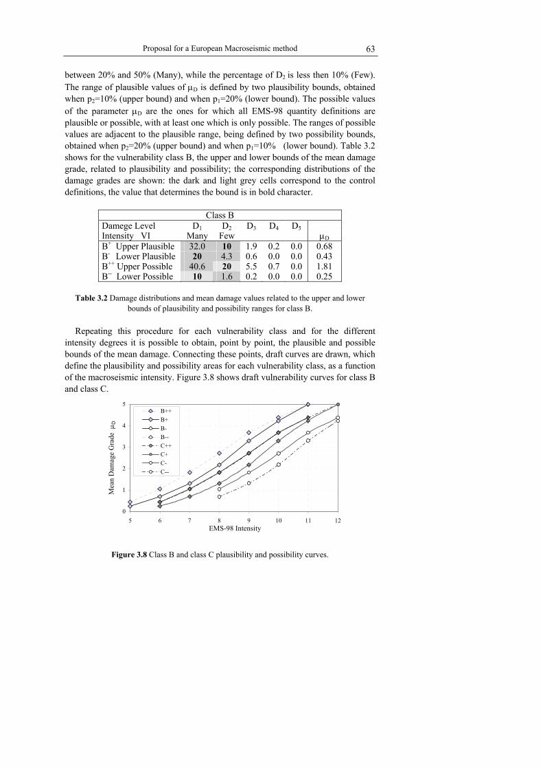
Proposal for a European Macroseismic method
63
between 20% and 50% (Many), while the percentage of D2 is less then 10% (Few). The range of plausible values of µD is defined by two plausibility bounds, obtained when p2=10% (upper bound) and when p1=20% (lower bound). The possible values of the parameter µD are the ones for which all EMS-98 quantity definitions are plausible or possible, with at least one which is only possible. The ranges of possible values are adjacent to the plausible range, being defined by two possibility bounds, obtained when p2=20% (upper bound) and when p1=10% (lower bound). Table 3.2 shows for the vulnerability class B, the upper and lower bounds of the mean damage grade, related to plausibility and possibility; the corresponding distributions of the damage grades are shown: the dark and light grey cells correspond to the control definitions, the value that determines the bound is in bold character.
Class B
Damege Level D1 D2 D3 D4 D5 Intensity VI Many Few µD B+ Upper Plausible 32.0 10 1.9 0.2 0.0 0.68 B- Lower Plausible 20 4.3 0.6 0.0 0.0 0.43 B++ Upper Possible 40.6 20 5.5 0.7 0.0 1.81 B-- Lower Possible 10 1.6 0.2 0.0 0.0 0.25
Table 3.2 Damage distributions and mean damage values related to the upper and lower
bounds of plausibility and possibility ranges for class B. Repeating this procedure for each vulnerability class and for the different
intensity degrees it is possible to obtain, point by point, the plausible and possible bounds of the mean damage. Connecting these points, draft curves are drawn, which define the plausibility and possibility areas for each vulnerability class, as a function of the macroseismic intensity. Figure 3.8 shows draft vulnerability curves for class B and class C.
0
1
2
3
4
5
5 6 7 8 9 10 11 12 EMS-98 Intensity
Mea
n D
amag
e G
rade
µD
B++B+B-B--C++C+C-C--
Figure 3.8 Class B and class C plausibility and possibility curves.

Chapter 3
64
3.2 VULNERABILITY INDEX AND VULNERABILITY CURVES
Observing the diagram of Figure 3.8, it stands out that there is a plausible area for each vulnerability class and intermediate possible areas for contiguous classes. In other words, the area between B+ and B- is distinctive of class B, while in the contiguous area the best buildings of class B and the worse of class C coexist (the B- curve coincides with the C++ one; the B-- curve coincides with the C+ one). Another important outcome of the analysis above presented, is that curves in Figure 3.8 are, more or less, parallel; this is because the damage produced to buildings of a certain vulnerability class, because of an earthquake of certain intensity, is the same caused by the following intensity degree to buildings of the subsequent vulnerability class. On the basis of these considerations, a conventional vulnerability index V (defined inside the fuzzy set theory), is introduced representing the belonging of a building to a vulnerability class. Vulnerability index numerical values are arbitrary; they are scores to quantify in a conventional way the building behaviour (they represent a measure of the weakness of a building to the earthquake). For the sake of simplicity a V=0÷1 range has been chosen, allowing to cover all the area of possible behaviour, being values close to 1 those of the most vulnerable buildings and values close to 0 the ones representative of the high-code designed structures.
Thus, the membership of a building to a specific vulnerability class can be defined by this vulnerability index (Figure 3.9); in compliance with the fuzzy set theory vulnerability index membership functions have a plausible range (χ=1) and linear possible ranges, representative of the transition between two adjacent classes.
0
0.5
1
-0.1 -0.02 0.06 0.14 0.22 0.3 0.38 0.46 0.54 0.62 0.7 0.78 0.86 0.94 1.02 1.1
Vulnerability Index V
Mem
bers
hip
Func
tion
χ
F ABCDEX Y
Figure 3.9 Vulnerability index membership functions for EMS 98 vulnerability classes. The fuzzy definition of the vulnerability index (Figure 3.9) is perfectly coherent
with the considerations previously done relatively to the vulnerability curves; the membership functions of the six vulnerability classes have the same shape and are translated of the same quantity, according to the parallelism and the constant spacing

Proposal for a European Macroseismic method
65
between the curves (Figure 3.8). According to the fuzzy definition of the vulnerability index, Table 3.3 shows the most probable value for each vulnerability class V0 (assumed according to a defuzzification process as the membership function χ centroid), the bounds (V-, V+) of the possibility range (χ=1), and the upper and the lower bound of its possible values (Vmin, Vmax). It must be noticed (Fig. 3.9) that the partition of the fuzzy field is not restricted to –0.02 as the minimum value and to 1.02 as the maximum value; actually it is not possible to keep out the chance of buildings weaker than the one belonging to class A or building better designed than the one classified as class F.
Vmin V- V0 V+ Vmax Vmin V- V0 V+ Vmax A 0.78 0.86 0.9 0.94 1.02 D 0.3 0.38 0.42 0.46 0.54 B 0.62 0.7 0.74 0.78 0.86 E 0.14 0.22 0.26 0.3 0.38 C 0.46 0.54 0.58 0.62 0.7 F -1.02 0.06 0.1 0.14 0.22
Table 3.3 Vulnerability index values for the vulnerability classes.
For the operational implementation of the methodology, an analytic expression
interpolating the curves in Figure 3.8 has been defined (3.11). The proposed vulnerability curve formula provides the mean damage grade µD as a function of the macroseismic intensity I, only depending from two parameters: the vulnerability index V and the ductility index Q.
DI 6.25V -13.12.5 1 tanh
Q +
µ = +
(3.11)
The vulnerability index V value determine the position of the curve; an increase
of V equal to ∆V=0.16 means that the same damage grade is produced by a one degree less earthquake. The ductility index Q determines the rate of increase in the damage with intensity. The curves derived from EMS-98 scale are characterized by Q=2.3.
3.3 VULNERABILITY INDEX DEFINITION FOR BUILDING TYPOLOGIES
Numerical and complete Damage Probability Matrices have been derived from EMS-98 Macroseismic Scale definitions for the 6 vulnerability classes considered by the scale (A ÷ F) and related vulnerability curves have been drawn (3.11).
The vulnerability model so derived, has been then referred directly to the building typologies, making reference to EMS-98 vulnerability table (Figure 3.10), which contains a typological classification representative of the various building types in the European countries. EMS-98 vulnerability table establishes a correspondence between vulnerability classes and building typologies (grouped for structural

Chapter 3
66
material in masonry, reinforced concrete, steel and wood typologies) as it recognises that the seismic behaviour of buildings, in terms of apparent damage, may be described making reference to the seismic behaviour of the six vulnerability classes. Thus, different types may behave in a similar way (see, for example, Massive Stone and Unreinforced Masonry with r.c. floors); on the other hand, it emerges that even if each type of structure is characterized by a prevailing vulnerability class, it is possible to find buildings with a better or worse seismic behaviour, depending on their constructive or structural characteristics and every other parameter able to affect their earthquake resistance. This is an original concept introduced by EMS-98 scale as in all the previous ones (included MSK 76) the correspondence between vulnerability classes and building typologies was considered in a deterministic way.
The idea highlighted by the EMS-98 scale, according to which the seismic behaviour of a building does not only depends on the behaviour of its structural system, but it involves other factors, has suggested the following definition of the vulnerability index:
0 r mV V + V + V= ∆ ∆ (3.12)
where 0V is a typological vulnerability index, rV∆ is the regional vulnerability factor, mV∆ represents a contribution to take into account the presence of seismic behaviour modifiers.

Proposal for a European Macroseismic method
67
Figure 3.10 EMS-98 building typologies and identification of their seismic behavior by vulnerability classes.
3.3.1 Typological vulnerability index
EMS-98 vulnerability table (Figure 3.10) describes the different belonging of a typology to a vulnerability class through the linguistic terms “Most possible class”, “Possible Class” and “Unlikely class” that, in the proposed approach, have been handled by the fuzzy set theory.
The membership function of each building type has been obtained as a linear combination of the vulnerability class membership functions, each one considered with its own degree of belongings (Figure 3.11). As an example, the membership function of the massive stone masonry M4 is so defined:
( ) ( ) ( ) ( )M4 C C CV V +0.6 V +0.2 Vχ = χ χ χ (3.13)
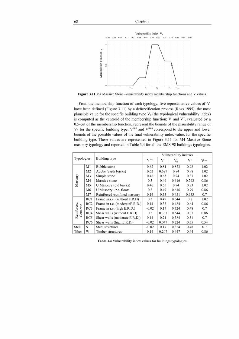
Chapter 3
68
00.
51
-0.02 0.06 0.14 0.22 0.3 0.38 0.46 0.54 0.62 0.7 0.78 0.86 0.94 1.02
Vulnerability Index VI
Mem
bers
hip
Func
tion
χ
VmaxV0V- V+Vmin Figure 3.11 M4 Massive Stone -vulnerability index membership functions and V values.
From the membership function of each typology, five representative values of V
have been defined (Figure 3.11) by a defuzzification process (Ross 1995): the most plausible value for the specific building type V0 (the typological vulnerability index) is computed as the centroid of the membership function; V- and V+, evaluated by a 0.5-cut of the membership function, represent the bounds of the plausibility range of V0 for the specific building type. Vmin and Vmax
correspond to the upper and lower bounds of the possible values of the final vulnerability index value, for the specific building type. These values are represented in Figure 3.11 for M4 Massive Stone masonry typology and reported in Table 3.4 for all the EMS-98 buildings typologies.
Vulnerability indexes
Typologies Building type minV V − 0V V + maxV M1 Rubble stone 0.62 0.81 0.873 0.98 1.02 M2 Adobe (earth bricks) 0.62 0.687 0.84 0.98 1.02 M3 Simple stone 0.46 0.65 0.74 0.83 1.02 M4 Massive stone 0.3 0.49 0.616 0.793 0.86 M5 U Masonry (old bricks) 0.46 0.65 0.74 0.83 1.02 M6 U Masonry - r.c. floors 0.3 0.49 0.616 0.79 0.86
Mas
onry
M7 Reinforced /confined masonry 0.14 0.33 0.451 0.633 0.7 RC1 Frame in r.c. (without E.R.D) 0.3 0.49 0.644 0.8 1.02 RC2 Frame in r.c. (moderateE.R.D.) 0.14 0.33 0.484 0.64 0.86 RC3 Frame in r.c. (high E.R.D.) -0.02 0.17 0.324 0.48 0.7 RC4 Shear walls (without E.R.D) 0.3 0.367 0.544 0.67 0.86 RC5 Shear walls (moderate E.R.D.) 0.14 0.21 0.384 0.51 0.7 R
einf
orce
d C
oncr
ete
RC6 Shear walls (high E.R.D.) -0.02 0.047 0.224 0.35 0.54 Stell S Steel structures -0.02 0.17 0.324 0.48 0.7 Tiber W Timber structures 0.14 0.207 0.447 0.64 0.86
Table 3.4 Vulnerability index values for buildings typologies.

Proposal for a European Macroseismic method
69
3.3.2 The behaviour modifier factor
As observed by EMS-98 macroseismic scale, the seismic behaviour of a building does not only depends on the behaviour of its structural system but it is affected by many other factors such as the quality of the construction, the height, the plan and vertical irregularity and the condition of maintenance.
Masonry Reinforced Concrete ERD Level Without Moderate High
Behavior modifier Vm Vm Vm Vm
Good -0.04 Good - - - State of preservation Bad +0.04 Bad +0.04 +0.02 0
Low (1÷2) -0.08 Low (1÷3) -0.02 -0.02 -0.02 Medium (3÷5) 0 Medium(4÷7) 0 0 0 Number of
floors High (≥6) +0.08 High (≥8 ) +0.04 +0.04 +0.04Wall thickness Wall distance Structural
system Wall connections
-0.04÷+0.04
Geometry Geometry +0.04 +0.02 0 Plan Irregularity Mass distribution
+0.04 Mass +0.02 +0.01 0
Vertical Irregularity
Geometry Mass distribution +0.04 Geometry
Mass +0.04 +0.02 0
Superimposed floors +0.04
Roof Weight, thrust and connections +0.04
Retrofitting Intervention -0.08÷+0.08
Aseismic Devices
Barbican, Foil arches, Buttresses -0.04
Middle -0.04 Corner +0.04
Aggregate Building: position Header +0.06
Insufficient aseismic joints
+0.04 0 0
Staggered floors +0.04 Aggregate Building: elevation
Buildings with different height -0.04÷+0.04
Beams -0.04 0 0 Connected 0 0 0 Foundation Different level
foundations +0.04 Isolated +0.04 0 0 Short-column +0.02 +0.01 0 Bow windows +0.04 +0.02 0
Table 3.5 Scores for behavior modifier factors for Masonry and RC buildings.
Modifying scores, Vm,k are therefore defined so that the typological vulnerability
index V0, computed for each typology can be increased or decreased on the basis of the vulnerability factors recognized inside a certain building.

Chapter 3
70
In Table 3.5 behaviour modifier factors and the corresponding scores Vm are proposed for Masonry and Reinforced Concrete buildings.
In order to take account of the influence of different behaviour modifiers on the building behaviour a behaviour modifier factor mV∆ is introduced in the computation of the final vulnerability index V.
The behaviour modifier factor mV∆ is evaluated according to (3.14) as the sum of the scores Vm,k of the recognized behaviour modifiers:
m m,kk
V V∆ = ∑ (3.14)
The behaviour modifiers identification has been made empirically, on the basis of
the observation of typical damage pattern, taking into account also what suggested by several Inspection Forms (ATC21 1988, Benedetti and Petrini 1984, UNDP/UNIDO 1985) and by previous proposal (Coburn and Spence 1992). The modifying scores Vm,k are attributed on the basis of expert judgment. They have been partially calibrated by the comparison with previous vulnerability evaluation; a further calibration is wished on the basis of damage and vulnerability data collected after earthquakes.
3.3.3 The regional vulnerability factor
The range bounded by V− , V+ is quite large in order to be representative of the huge variety of the constructive techniques used all around the different European countries.
A regional vulnerability factor ∆Vr is introduced to take into account the typifying of some building typologies at a regional level: a major or minor vulnerability could be indeed recognized due to some traditional constructive techniques for building classified as belonging to same building typology or vulnerability class in different regions.
According to this regional vulnerability factor ∆Vr it is allowed to modify the V0 typological vulnerability index on the basis of an expert judgment or on the basis of the available historical data. The first case is achieved when precise technological, structural, constructive information exist attesting an effective better or worse average behaviour with regard to the one proposed in Table 3.4. The second one occurs when data about observed damages exist; the average curve can be shifted in order to obtain a better approximation of the same data (Figure 3.12).

Proposal for a European Macroseismic method
71
0
1
2
3
4
5
5 6 7 8 9 10 11 12
EMS-98 Intensity
Mea
n D
amag
e G
rade
µD
M4-
M4*
M4+
Lisbon
M4*+DeltaVr
Figure 3.12 According to Oliveira (1984) M4 Massive Stone typology in Lisbon could provide a better behavior than the proposed average one (Table 4): a ∆VR=0.12 is applied. The final vulnerability index V accounting for the contribution of the behaviour
modifiers factor ∆Vm and of the regional factor ∆Vr according to (3.12) has to comply with the possibility range:
( ) ( )max min 0 0 Max V ;V V Min V ;V≤ ≤ (3.15)
3.4 THE UNCERTAINTY AFFECTING THE VULNERABILITY ASSESSMENT
It is recognized how vulnerability evaluations (Spence et al. 2003) are affected by uncertainties associated with the classification of the exposed building stock into vulnerability classes or into building typologies and by uncertainties associated with the attribution of a characteristic behaviour to each vulnerability class or to the building typology. Both these two sources of uncertainties are recognized by EMS98 scale that, as a matter of fact, describes the seismic performance of six vulnerability class (from A to E) by linguistic definitions that are as well employed in order to correlate the seismic performance of building typologies to the one of vulnerability classes.
The use of fuzzy logic theory for the translation of the linguistic definitions provided by the scale has allowed quantifying the cognitive uncertainty characterizing vulnerability class and building typology behaviours in terms of membership function of the vulnerability index V. According to its fuzzy definition a most probable value for the vulnerability index V0 is provided together with uncertainty range around it (bounded by an upper Vmax and a lower values Vmin) for each vulnerability class (Table 3.3) and for each building typology (Table 3.4).

Chapter 3
72
It must be noticed how the uncertainty range around V0 is higher for building typologies than for vulnerability classes; thus as the building typology behaviour has been deduced from the one observed from vulnerability classes and furthermore because with few data is more difficult to classify a building into a typology rather than into a vulnerability class.
Considering that the knowledge of additional information, then the typological ones, limits the uncertainty about the building behaviour, it has been considered advisable not only to modify the most probable value V0 (according to Equation 3.12), but also to reduce the range of its uncertainty Vmin÷ Vmax. This goal has been achieved modifying the membership function through a filter function f, centred on the final vulnerability index value:
f
0 m r f 0 m r
0 m r f0 m r f 0 m r f
f
0 m r f
∆V(V,V ,∆V ,∆V , V ) 1 if V V V ∆V
2V V V V ∆V 3(V,V ,∆V ,∆V , V ) 1.5- if V V V ∆V ∆V
∆V 2 2
(V,V ,∆V ,∆V , V ) 0
∆ = − − ∆ − ≤
− − ∆ − ∆∆ = ≤ − − ∆ − ≤
∆ =
f
f
f 0 m r f f3 if V V ∆V ∆V V ∆V 2
− − − − ∆ >
(3.16)
The filter function is multiplied by the membership function of an EMS-98
typology and the resulting function is afterwards normalized to a maximum value equal to 1, so obtaining the membership function of the specific set of buildings, which takes into account all the vulnerability factors:
[ ]
0 m f
0 m f
(V) (V,V ,∆V ,∆V )(V)
max (V) (V,V ,∆V ,∆V )=
ff
χχ
χ (3.17)
The filter function is function of the parameter ∆Vf, that represents the width of
the filter function, and it is defined depending on the quantity and quality of the available data. In Table 3.6 two possible proposals are shown.
DATA ORIGIN
fV∆ Non specified existing data base 0.08 Data specifically surveyed for vulnerability purposes 0.04
Table 3.6 fV∆ suggested values depending on data origin and quality.
For the sake of an easier operative application of the methodology the filter
function can be substituted with an acceptable approximation directly considering, around the final vulnerability index value V, an uncertainty range with a width equal to the value suggested in Table 3.6:

Proposal for a European Macroseismic method
73
0 f
0 f
3V V V23V V V2
+
−
= + ∆
= − ∆
(3.18)
3.5 EMS-98 MACROSEISMIC INTENSITY: THE EARTHQUAKE SIZE FOR THE PROPOSED MACROSEIMIC METHOD
The Macroseismic Intensity is the most natural parameter to represent seismic input dealing with vulnerability methods derived from damage observation. Considering how the proposed method has been obtained, EMS-98 Macroseismic Intensity is the input parameter to make reference to for the proposed macroseismic method.
Different critics have been advanced on the use of macorseismcic intensity for vulnerability and loss assessment models. One of the first is that Macroseismic intensity scale is discrete by definition, as only integer values are permissible. Secondly it is remarked that a macroseismic measure is subjective-based on the synthesis of the personal judgements of many observers, resulting in a qualitative measure. Moreover it is said that a macroseismic measure is limited depending on the assessment of particular building types and phenomena, and particular level of damage.
The objection that intensity is not a valid parameter to characterize seismic input, being a discrete quantity, may be overcome, bearing in mind that, even intermediate values, conceptually lacking in meaning in a macrosesimic survey, may be used for forecast purposes; in the proposed model, intensity is considered as a continuous parameter and as well, regarding hazard scenarios, intensity attenuation laws provide continuous values.
With regard to the criticism about its qualitative nature, it is true that the evaluation of an intensity hazard scenario cannot take advantage from the considerable developments of seismological research for the definition of physical-mechanical seismic input representation (i.e. the progresses made in the field of modeling of mechanisms of source, of the propagation of waves and of seismic microzoning), that, on the contrary, a physical-mechanical hazard definition (PGA, displacement and acceleration spectrum) can make use of. By the consciousness that employing Intensity a set of knowledge is overlooked on respect to a physical mechanical hazard representation, a higher amount of uncertainty should be considered in the hazard description.
On the others hand, the advantages and the potentiality that the employment of Macroseimic Intensity offers has not to be foregone (Par. 2.2.1.2). First of all, it is univocally recognized that intensity remains an important reference parameter in seismic risk studies as, only by means of intensity, it is possible to make use of the essential information contained in the catalogues of historical seismicity. Secondly, a macroseismic measure let to characterise ground motion on larger areas than the ones covered by instruments.

Chapter 3
74
3.6 SITE EFFECTS INCREASING THE BUILDING VULNERABILITY
Nevertheless these considerations on behalf of Macroseismic Intensity, this parameter is, for the physical characterization of the seismic input, definitely less meaningful than PGA and than displacement or acceleration spectra. On respect to PGA, the use of Macroseismic Intensities does not allow to represent soil amplification. On the other hand, whit regard to the structures, it is comparable to a PGA (Peak Ground Acceleration) representation, that, non-released from a spectrum does not provide any information about the dynamic behaviour of a structure.
For hazard scenarios represented in terms of macroseismic intensity, soil amplifications are usually taken into account increasing, locally, the intensity evaluated on rock (TC4-ISSMFE 1993).
Anyway, the undifferentiated increase on Intensity for a certain soil type is incorrect, as it does not allow taking into account the differences in the dynamic amplification connected with the fundamental frequencies of both the soil and the structure. In order to overcome this limitation, it is proposed, in the follow, to consider this possible dynamic amplification in term of a soil vulnerability index modifier ∆Vs (Giovinazzi and Lagomarsino, 2004). The vulnerability index modifiers ∆Vs, defined in order to take into consideration soil amplification effects, have been evaluated considering jointly soil conditions and the characteristic of the built environment (masonry and reinforced buildings are distinguished and their height is taken into account).
To each building typology a fundamental period T has been ascribed making reference to EC8 (CEN 2003). T is evaluated for Masonry and Reinforced Concrete categories for three different ranges of height (low, medium, high):
0.75
tT C H= (3.19)
where Ct=0.075 for moment resistant space concrete frames and Ct=0.05 can be assumed for masonry structure. The building height H[m] is evaluated assuming for each category the number of floor in table 3.7 and considering an average interstory height h=3m.
M-Low M-Medium M-High RC-Low RC-Medium RC-High Floors 2 4 6 3 7 12 T1 0.19 0.32 0.44 0.39 0.74 1.10
Table 3.7 Fundamental period T for Masonry and RC buildings.
With regard to the soil, the ground classes defined by EC8 (2003) (Table 2.11)
have been considered. To different soil conditions different elastic response spectra are related provided by discrete value for fixed period or by predefined spectral shape as in case of EC8 elastic response spectra.

Proposal for a European Macroseismic method
75
For the assumed spectral shape, a PGA multiplier factor fPGA is evaluated that generate a seismic action able to produce on a certain building category (T1 fixed) built on a certain soil (ground class k), the same effect as if it was built on Rock (ground class A). In others words, making reference to the response spectrum related to rock soil condition, the PGA multiplier factor, able to generate for a given building period T the same seismic action that it would be caused by different soil conditions (ground class k), is evaluated.
( )( )
ae (k)ag
ae (A)
S Tf
S T= (3.20)
3.6.1 Site effect vulnerability factor derived from EC8 horizontal elastic response spectrum
EC8 defines the acceleration elastic response spectrum Sae(T) for the horizontal components of the seismic action by the following expression:
( )g BB
g B C
aeC
g C D
C Dg D2
Ta S 1 2.5 1 0 T TT
a S 2.5 T < T TS (T) T
a S 2.5 T < T TTT T
a S 2.5 T < T 4sT
η + η − ≤ ≤
η ≤= η ≤
η ≤
(3.21)
where Sae(T) is the acceleration elastic response spectrum, T is the vibration
period of a linear single-degree-of-freedom system, ag is the design ground acceleration on soil type A, TB and TC are the bounds of the constant spectral acceleration branch, TD defines the beginning of the constant displacement response range of the spectrum, S is soil factor and η is the damping correction factor with a reference value η=1 for 5% viscous damping. The values of TB, TC and TD periods and the value of S soil factor, defining the shape of the elastic response spectrum, depend on the ground type. EC8 provides these parameters differently depending on the size of the surface-wave magnitude Ms that is supposed to have generated the earthquake. A Type 1 spectrum is introduced when the earthquakes that contribute most to the seismic hazard definitions are characterized by a surface-wave magnitude Ms greater than 5.5 (Ms>5.5) . When the surface-wave magnitude Ms is non greater then 5.5 (Ms<5.5) a Type 2 spectrum is recommended. Table (3.8) shows the values of the parameters defining EC8 Type 1 and Type 2 spectra.

Chapter 3
76
Type 1 Type 2 Ground S TB TC TD Ground S TB TC TD
A 1,0 0,15 0,4 2,0 A 1,0 0,05 0,25 1,2 B 1,2 0,15 0,5 2,0 B 1,35 0,05 0,25 1,2 C 1,15 0,20 0,6 2,0 C 1,5 0,10 0,25 1,2 D 1,35 0,20 0,8 2,0 D 1,8 0,10 0,30 1,2 E 1,4 0,15 0,5 2,0 E 1,6 0,05 0,25 1,2
Table 3.8 Values for the parameters defining the recommended EC8 Type 1 and Type 2
elastic response spectrum.
According to the definition provided by EC8 for the elastic response spectrum (3.21), the multiplier factors (3.20) of the peak ground accelerations for different ground conditions (k) on respect to ground class A are evaluated as follow:
g
B(k)B(A) (k)B
B(k) (A) B(A)
(k)B C
(A)a
(k) C(k)C
(A) C(A)
T T(2.5 -1)T S 0 T T
T S T T(2.5 -1)
S T < T T
Sf
S T T < T
S T
+ η ≤ ≤ + η
≤=
D
(k) C(k) D(k)D
(A) C(A) D(A)
T
S T T T < T 4s
S T T
≤ ≤
(3.22)
3.6.1.1 Site effect vulnerability factor for EC8 Type1 spectrum
Making reference to EC8 elastic response spectrum (3.21) and to the values provided for the parameters of Type 1 spectum (Table 3.8), fag factors have been evaluated according to (3.22) for the building categories in Table 3.7.
The results are provided in Table 3.9 for B, C, D and E, EC8 ground classes.

Proposal for a European Macroseismic method
77
0
0.5
1
1.5
2
2.5
0 0.2 0.4 0.6 0.8 1 1.2 1.4 1.6 1.8 2T(s)
Sae[
m/s
2]
Sae Ground ASae Ground DSae -CA Low - Ground ASae -CA Medium - Ground ASae CA High - Ground AT1 CA LowT1 CA MediumT1 CA High
Figure 3.13 Type 1 Elastic Response Spectra for Ground A able to reproduce the same
seismic action suffered by reinforced concrete building of different height built on Ground D.
fag fag Soil Class B C D E Soil Class B C D E M-Low 1.2 1.15 1.35 1.4 RC-Low 1.2 1.15 1.35 1.4 M-Medium 1.2 1.15 1.35 1.4 RC-Medium 1.5 1.725 2.5 1.75M_ High 1.32 1.265 1.485 1.54 RC-High 1.5 1.725 2.7 1.75
Table 3.9 PGA multiplier factors fag evaluated for EC8 Type 1 Spectrum, for the different soil
classes and for different building categories. According to I-ag correlations (Par.2.2.3.1) an Intensity Increment ∆I corresponds
to a peak ground acceleration multiplier factor fPGA. In particular ∆I increments shown in Table 3.11 have been evaluated employing Guagenti & Petrini (1989) I-ag correlation (2.2).
agln(f )I
0.602∆ = (3.23)
∆I ∆I B C D E B C D E M_Low 0.30 0.23 0.5 0.56 RC_Low 0.30 0.23 0.5 0.56M_Medium 0.30 0.23 0.5 0.56 RC_Medium 0.67 0.91 1.52 0.93M_High 0.46 0.39 0.66 0.72 RC _High 0.67 0.91 1.65 0.93
Table 3.10 Intensity Increments ∆I evaluated for EC8 Type1 Spectrum, for the different soil
classes and for different building categories. According to the formula proposed for vulnerability curves description (3.11), a
variation of the vulnerability index ∆V corresponds to the macroseimic intensity variation ∆I (3.24):

Chapter 3
78
IV6.25∆
∆ = (3.24)
Thus making reference to the computed ∆I increments (Table 3.10) vulnerability
index soil modifiers ∆Vs, for different building typologies, classes of height and ground types, can be evaluated according to (3.24). Results are shown in Table 3.11.
∆Vs ∆Vs B C D E B C D E M_Low 0.04 0.03 0.08 0.09 RC _Low 0.04 0.03 0.08 0.09M_Medium 0.04 0.03 0.08 0.09 RC_Medium 0.10 0.15 0.24 0.15M_High 0.07 0.06 0.10 0.12 RC_High 0.10 0.15 0.26 0.15
Table 3.11 Vulnerability increments ∆Vs evaluated for EC8 Type I spectrum, for the different
soil classes and for different building categories.
3.6.1.2 Site effect vulnerability factor for EC8 Type 2 spectrum
The procedure has been repeated for Type 2 spectrum assuming EC8 recommended values for the five parameters S, TB, TC and TD in Table 3.8. Table 3.12 shows the resulting peak ground acceleration multiplier factors fag.
fag fag B C D E B C D E M-Low 1.35 1.5 1.8 1.6 RC-Low 1.35 1.5 2.16 1.6M-Medium 1.35 1.5 2.16 1.6 RC-Medium 1.35 1.5 2.16 1.6M_ High 1.35 1.5 2.16 1.6 RC-High 1.35 1.5 2.16 1.6
Table 3.12 PGA multiplier factors fag vulnerability increments ∆Vs evaluated for the
Response Spectrum derived from AMB96 predictive equations. On respect to fag computed for Type 1 spectrum (Table 3.9), the peak ground
acceleration multiplier factors fag evaluated for Type 2 are higher for all the building categories except for medium and high reinforced concrete buildings.
Intensity increment ∆I corresponding to these peak ground acceleration multiplier factors fag, have been obtained employing Guagenti and Petrini (1989) I-ag correlation (2.2) and vulnerability index soil modifiers ∆Vs (Table 3.13) have been evaluated applying (3.24).

Proposal for a European Macroseismic method
79
∆Vs ∆Vs B C D E B C D E M_Low 0.08 0.10 0.15 0.12 RC _Low 0.08 0.10 0.20 0.12M_Medium 0.08 0.10 0.20 0.12 RC_Medium 0.08 0.10 0.20 0.12M_High 0.08 0.10 0.20 0.12 RC_High 0.08 0.10 0.20 0.12
Table 3.13 Vulnerability increments ∆Vs evaluated for EC8 Type 2 Spectrum, for the
different soil classes and for different building categories.
3.6.2 Site Effect vulnerability factor derived from predictive equations
Soil conditions vulnerability index modifier ∆Vs can be as well evaluated in the case response spectra are provided by discrete values for fixed periods, as for instance when hazard scenarios are evaluated making reference to spectral ordinate predictive equations. Considering the general formulation provided in (2.13) for PGA or spectral ordinate predictive equations, the dependence of the soil amplification factor on the structural fundamental period T can be evaluated as follow:
kag
A
Y(T,soil )f
Y(T,soil )= (3.25)
Figure 3.14 portrays this ratio (dependence of site amplification on the T) for soil
category C and for different attenuation relationships. It can be noticed how for T=0 [s] the amplification is about fag=1.3, while the largest soil amplification, about fag =1.7, occurs at T around T=1[s]. It can be, as well, noticed the significantly different amplification behaviour of shallow soil deposits with respect to deep ones.
1
1.1
1.2
1.3
1.4
1.5
1.6
1.7
1.8
1.9
2
0 0.5 1 1.5 2 2.5Period T
Amplificator factorBoore et al. 1997
Ambraseys et al. 1996
Sabetta & Pugliese1996 (shallow alluvium)Sabetta & Pugliese1996 (deep alluvium)
Figure 3.14 Response spectral amplification factors for soft soil (Category C) and
deep/shallow soil sites with respect to rock sites as a function of oscillator period for different attenuation relations (from Faccioli and Pessina, 2003).

Chapter 3
80
In the following the procedure for determine the soil vulnerability index modifier ∆Vs is developed for AMB96 (2.15) attenuation law, which provides acceleration response spectral values (Sae) and makes use of a simplified classification into 4 ground classes (from rock to very soft soil listed in table 3.14 depending on shear wave velocity Vs30) almost coincident with EC8 soil classification (Table 2.11).
Rock (R) Stiff soil (A) Soft soil (S) Very Soft Soil (L) VS30 >750 360-750 180-360 <180
Table 3.14 Classification of ground conditions according to AMB96.
Table 3.15 shows the results obtained in terms of peak ground acceleration
factors fag for building categories in Table 3.7 and the corresponding soil vulnerability index modifier ∆Vs in the hypothesis to correlate fag to ∆I by Guagenti and Petrini (1989) correlation (2.2). It is worth to highlight that these factors are invariable for different earthquake magnitude M and site-source distances R.
fag ∆Vs fag ∆Vs
Stiff Soft Stiff Soft Stiff Soft Stiff Soft M-Low 1.33 1.45 0.08 0.10 RC-Low 1.42 1.54 0.09 0.11M-Medium 1.36 1.46 0.08 0.10 RC-Medium 1.33 1.68 0.08 0.14M_ High 1.33 1.63 0.08 0.13 RC-High 1.28 1.61 0.07 0.13
Table 3.15 PGA multiplier factors fag evaluated for EC8 Type1 Spectrum, for different soil
classes and for different building categories
Comparing these fag values with the ones previously evaluated for EC8 spectra, it can be noticed that they are lower and less invariant depending on the structural period on respect to the fag derived from Type 1 spectrum. A good agreement is observed on respect to fag derived from EC8 Type 2 spectrum. On the other hand, both peak ground acceleration factors fag and macroseimic intensity increments ∆I are consistent with the proposal found in literature, respectively with amplification factor defined by Midorikawa (1987) (Table 2.13) and with intensity increments proposed by Evender and Thomson (1985) (Table 2.12).
3.7 MACROSEISMIC METHOD IMPLEMENTATION FOR DIFFERENT SCALES AND EMPLOYING DATA OF DIFFERENT QUALITY AND DETAIL
A valuable feature of the proposed Macroseismic method is that it can be implemented for different scale of analysis starting from data of various origin and quality. In the following the operative aspects of data processing are discussed making reference to different conditions of data availability and detail of the analysis.

Proposal for a European Macroseismic method
81
3.7.1 Processing the available data for the vulnerability index evaluation
In order to evaluate the parameters defining the macroseismic vulnerability index V, any available database related to buildings can be taken into consideration. Moreover all the knowledge about observed vulnerability, traditional constructive techniques together with the available local expert opinions have to be collected, as they can represent a useful source of information for the Macroseismic method implementation. The quantity and the quality of the knowledge available on the built environment, affect all the parameters involved in the vulnerability analysis and the amount of uncertainty characterizing the results.
One of the first step to move, processing available data on buildings, it is to asses what is the minimum unit of data availability, that means to understand if data exist for each single building, for a set of building (i.e. a building aggregate) or for geographycal area. In these last cases data are usually in the form of statistical information.
The distribution of the knowledge, namely the minimum unit on the territory for which data are available, leads up to the minimum unit to make reference to for performing the analysis referred in the following as “analysis unit”. This can be, indifferently, a single building, a building aggregate or a macro area containing several buildings (such as a district or a census tract).
In order to obtain a geographycal representation of the analysis performed by the Macroseicmic method, data need to be geocoded. Existing digital cartography have to be collected for this purpose or raster cartography have to be properly digitalized. The current position of geocoding is such that municipality and census tract boundary are available for almost all the European regions. The minimum geocoded unit in the found cartography (referred as “representation unit”) has to be identified as the unit to make reference to for the representation of data and results.
It is important to highlight that the resolution detail in data storage does not necessary correspond with the resolution to which reference is made for the analysis and the results representation: inside a GIS environment data may be aggregated and disaggregated. Indeed if data are available with a resolution higher then the geographycal representation, data contained in the representation unit have to be aggregated. On the contrary, if data are available for area wider then the ones represented, data belonging to the analysis unit have to be split between the contained representations units, following the criterion judged more suitable.
Once the analysis unit and the unit of data representation are identified, a data processing has to be performed in order to understand the consistency of the available information and how they could be useful for the vulnerability index evaluation.
First of all it is necessary to understand if existing data can lead to the typological identification of the buildings or of the set of buildings according to the proposed typological classification. Data useful to this aim are the vertical and horizontal structure types, the code level, the presence of a soft-story or the presence of retrofit

Chapter 3
82
interventions. The typological identification leads to the attribution of the typological vulnerability index V0 according to Table (3.4). If data are insufficient for this purpose, inferences have to be established between more general data and a distribution of building typologies, in order to identify building categories. A basic vulnerability index is so ascribed to the identified categories VC
0, equivalent to V0. Any other parameters eventually available for a deeper knowledge should have led back to one of the proposed vulnerability index modifiers in order to evaluate the behaviour modifier factor ∆Vm (Par 3.3.2).
Moreover, any availability of field or laboratory tests on the constructive materials, aiming to identify their mechanical characteristics, and any detailed typological analysis, aiming to asses the traditional constructive features and the rules of thumbs, should have taken into consideration for the attribution of a possible regional modifier factor ∆Vr (Par 3.3.3). To this aim observed damage data for the building typologies identified on the territory are as well useful.
Finally, a judgment about the quality and the reliability of the available data has to be stated, in order to understand the possibility to reduce the uncertainty in the vulnerability assessment by the ∆Vf parameter (Par 3.4). Expert judgement plays an important role on the ∆Vf attribution as it goes without saying that not necessarily data specifically surveyed for vulnerability purposes are more reliable than data coming from other sources that could be wider, very detailed and accurate.
Table 3.16 summarizes data features to be identified performing the data processing and how the different information affects the macroseimic method parameters.
Data features Parameters
Single building Minimum unit of data availability Set of buildings
Analysis Unit
Direct typological identification Data consistency Direct typological identification by inferences V0
Data consistency Number of behaviours modifiers ∆Vm Observed vulnerability Existing knowledge Expert judgment ∆Vr
Specific survey with vulnerability assessment purposes. Data origin Other origins
∆Vf
Single building Minimum geocoded unit Set of buildings
Representation Unit
Table 3.16 Building data meaningful for the vulnerability index V evaluation.
If the data processing highlights that some information are lacking or that the
necessity for a check or a deepening of the available data exists or, moreover, if no

Proposal for a European Macroseismic method
83
data are available at all, a field survey should be performed (compatibly with time and money availability) carried out through a rapid visual inspection.
3.7.2 Vulnerability index evaluation for single building and for set of buildings
If the analysis unit is identified with the single building, the typological vulnerability index V0 is directly ascribed to each of them according to Table (3.4) when data allow identifying the building typology. Otherwise, if reference has to be made to building categories, an equivalent V0 for the category V0
C can be evaluated coherently with the fuzzy logic by the union of building typologies membership function and by a subsequently defuzzification process (3.26) (Giovinazzi and Lagomarsino, 2003).
( )i
C0 i 0
i
V p V U→ µ (3.26)
where pi is the percentage for the i-building typology in defining the category
according to the assumed inference (Table 2.9). Alternatively, with a negligible mistake, the basic vulnerability index for the
category V0C can be computed as a weighted average (on respect to pi) of the
building typologies vulnerability indexes. The attribution of the regional vulnerability factor ∆Vr and of the behaviour
modifier factor ∆Vm for a single building is directly made according to what specified in Par. 3.3.2 and in Par. 3.3.3. The attribution of the soil vulnerability factor ∆Vs, is made according to the constructive material (masonry or reinforced concrete), the building height and the soil class recognized for the ground (Par. 3.6).
If the analysis unit is a set of building rather then a single building, the evaluation of the basic vulnerability index for the set making reference to building typologies V0_set or to building categories V0
C_set is computed taking into account the ratio of the
buildings inside the set supposing to belong to each building typology or to each building category (Table 3.7).
In the same way, the attribution of the regional vulnerability factor ∆Vr_set to a set of buildings depends on the ratios of buildings recognized as belonging to a specific building typology affected by the recognized ∆Vr. Identically the attribution of the behaviour modifier factor ∆Vm_set depends on the ratios of buildings characterized by the modifying factor k.

Chapter 3
84
Single Building Set of buildings
Typology V0 Values from Table ( 3.4)
0 set t 0 tt
V q V∑_ , =
Where qt is the ratio of buildings inside the set supposing to belong to a certain building typology. V0
Category V0
C Evaluated according to equation (3.26)
C C0 set c 0 c
cV q V_ , = ∑
Where qc is the ratio of buildings inside the set supposing to belong to a certain building category.
∆Vm Typology/ Category
m m kk
V V , = ∆ ∑
Values from Table (3.5)
m k m kk
V r V∆ ∑ , =
Where rk is the ratio of buildings characterized by the modifying factor k, with score Vm,k when a set of building is considered.
∆Vr Typology/ Category
r r kk
V V , = ∆ ∑
From expert judgment or observed vulnerability data
r k r kk
V r V∆ ∑ , =
Where rk is the ratio of buildings recognized as belonging to a specific typology t affected by the recognized Vr,k
∆VS Typology/ Category
∆Vs Values from Tables (3.11) (3.13) (3.15)
M j RC js j S j SV m V rc V, ,
3 3
j=1 j=1 = ∆ ∆ + ∆∑ ∑
Where mj and rcj are respectively the ratio of masonry and reinforced concrete recognized as belonging to a specific class of height (j=1 low, j=2 medium, j=3 high).
Table 3.17 Formula for vulnerability index evaluation for single buildings and for set of
buildings.
3.8 VULNERABILITY INDEX DEFINITION FOR HISTORICAL AND MONUMENTAL BUILDINGS
All ancient masonry buildings, including the biggest and most important monuments, have been constructed following the rule of thumb, learning from the experience of previous similar structures. Earthquake is a rare action and the builders experience was different from area to area and from time to time. In areas of high seismicity, where significant earthquakes occur quite often, buildings are characterized by constructive details and reinforcements specifically adopted to protect from seismic actions. In areas of moderate seismicity, these solutions may be found only in the buildings constructed immediately after a big earthquake, together

Proposal for a European Macroseismic method
85
with traditional repairing techniques (tie rods, buttresses, scarp walls, foil arches between facing buildings); however, the awareness of the importance of these details disappear after two or three generations.
Minor buildings in the historical centres are usually very vulnerable due to the low quality of masonry material, the poor state of maintenance and the successive transformations (obstructions, raising up of buildings, partial demolitions).
Monumental buildings are equally vulnerable, even thought for different reasons. Indeed, they are usually made by good quality materials, but their dimensions are significant: wide halls, thin long span vaults, slender towering or projecting parts, slender walls with large openings.
It is clear the necessity for suitable models for their vulnerability evaluation providing useful information for planning interventions and strategies for the risk mitigation and the emergency management. The importance and uniqueness of both monumental structures and historical centres may advice to deal with the problem of seismic vulnerability by a detailed seismic analysis on each single building. However, due to the large number and the high density of monuments that are present in prone seismic areas, even for the cultural heritage, seismic vulnerability is a problem that must be faced at territorial scale.
For this reason, the possibility to employ the proposed macroseimic method, originally derived for ordinary buildings, for historical centres and monumental buildings vulnerability assessment has represented an important achievement.
3.8.1 Vulnerability index definition for monumental buildings
Also in the case of monumental buildings, a vulnerability model suitable for application at the territorial scale has to be referred to a typological classification. Considering the wide variety of the artefacts that constitute the cultural heritage in the world, according to geographic location, architectural styles and ages of construction, this classification is not a straightforward task. However, for the sake of a simplified structural evaluation of the seismic vulnerability on a wide population of monuments, a typological classification is usually possible, gathering into groups the structures which are similar with reference to the architecture and the seismic behaviour. An example of a typological classification that may be considered as a reference for monuments in European countries is the following: palace, church, monastery and convent, mosque, tower, obelisk, theatre, castle, triumphal arch, arch bridge.
For historical buildings it has been possible to make reference to the same analytical function (3.11) employed for the description of ordinary building vulnerability curves (Lagomarsino and Podestà 2004b). Indeed this curve for different values of the parameters Q and V has proved to well fit the mean damage obtained from the damage distribution collected for churches during the last twenty years (Lagomarsino and Podestà 2004b, 2004c). In particular for churches the vulnerability index V assumes values between 0.67 and 1.22 (for the more

Chapter 3
86
vulnerable churches) while the ductility index Q assumes the value 3. Monumental palaces may be, on average, associated to massive stone building
typology, because their construction is typically characterized by good quality materials and craftsmanship. For massive stone buildings V0=0.62 (Table 3.4), and the vulnerability index may vary, according to the vulnerability scores, between 0.3 and 0.86 (a plausible range is 0.49<V<0.79).
It is worth noting that the vulnerability curves of churches and palaces are similar, with the exception of denominator, which controls the rate of increase of the damage with the intensity. The vulnerability curves of the churches and of the monumental palaces are compared in Figure 3.15. Due to higher values, on average, of the vulnerability index, churches turns out to be more vulnerable for the lower intensities; actually, in the case of minor earthquakes in Italy, the churches always exhibited an higher damage among the built environment. The higher ductility of the churches (Q=3 for churches, Q=2.3 for palaces) determines that for higher intensities, the seismic response tends to be similar to the one of the palaces.
0
1
2
3
4
5
5 6 7 8 9 10 11 12I
µ D
PalaceChurch
Figure 3.15 Vulnerability curves for palaces and churches (mean value, plausible range).
0
1
2
3
4
5
5 6 7 8 9 10 11 12I
µ D
PalaceObelisk TowerTheatreCastle
0
1
2
3
4
5
5 6 7 8 9 10 11 12I
µ D
ChurchMonasteryMosqueTriumphal archArch bridge
Figure 3.16 Mean vulnerability curves for monumental building typologies.

Proposal for a European Macroseismic method
87
Reference values for the other monumental types have been deduced from the ones defined for palaces and churches applying an expert judgement procedure (Table 3.18, Figure 3.16).
Typology V0 Q Palace 0.62 2.3 Church 0.89 3.0 Monastery/Convent 0.74 2.3 Mosque 0.81 2.6 Tower 0.78 2.0 Obelisk 0.74 3.0 Theatre 0.70 2.3 Castle 0.54 2.0 Triumphal arch 0.58 2.6 Arch bridge 0.46 2.3
Table 3.18 Vulnerability index V and ductility index Q for historical buildings.
3.8.1.1 Monumental building behaviour modifier
It is evident that a vulnerability index assigned to a monument simply by a typological classification represents an average value, which does not take into account the distinctiveness of the single building and does not allow singling out the most vulnerable structures among buildings of the same type. To refine the vulnerability assessment a quick survey is at least necessary, with the purpose of collecting by proper survey forms some relevant parameters, such as: state of maintenance, quality of materials, structural regularity (in plan and in elevation), size and slenderness of relevant structural elements, interaction with adjacent structures, presence of retrofitting interventions, site morphology.
Vulnerability scores Vk may be awarded to each one of the above mentioned parameters (Table 3.19) and the vulnerability index of each monument may be refined modifying the typological value (3.12), where the summation of behaviour modifier scores is extended to all the available modifiers (3.14).
Parameter Vk
state of maintenance very bad (0.08) – bad (0.04) – medium (0) – good (-0.04) quality of materials bad (0.04) – medium (0) – good (-0.04) planimetric regularity irregular (0.04) – regular (0) – symmetrical (-0.04) regularity in elevation irregular (0.02) – regular (-0.02) interactions (aggregate) corner position (0.04) – isolated (0) – included (-0.04) retrofitting interventions effective interventions (-0.08) site morphology ridge (0.08) – slope (0.04) – flat (0)
Table 3.19 Vulnerability scores Vk reference values for different parameters.

Chapter 3
88
The vulnerability scores may assume different values for different typologies; moreover, some relevant information may be distinctive only for one typology (i.e. the presence of a raising façade in churches). Table 3.20 shows, for instance, specific vulnerability parameters and modifying score values for churches.
Parameter Vk
Plan regularity: nave typology central (0.02) – one (0) – three (+0.02) Section regularity: raising elements or façade yes (0.04) – no (0) Position included (-0.02),additions (+0.02),isoleted (0)Domes/Vaults yes (0.04) – no (0)) Lateral walls height (low [< 6 m], medium [ > 6 m and < 12 m], high (> 12 m])
low (0.04) – isolated (0) – included (-0.04)
Table 3.20 Specific vulnerability parameters and modifying score values for churches. The choice of the specific vulnerability parameters has been made empirically, on
the basis of the observation of the typical damage of each monumental typology.
3.8.2 Vulnerability index definition for historical centre
The vulnerability elements towards a seismic action for building aggregates have been identified on the basis of damage observations (Giuffrè 1993, Guerrieri 1999).
Some of the elements causing the seismic vulnerability of building aggregates corresponds to weaknesses of each single building, while some others are directly connected with the aggregate context in which the building is inserted and some furthers are linked to the old age of the buildings and to the rules of thumbs constructive techniques employed (Figure 3.17).
Figure 3.17 Examples of damage patterns for building belonging to historical centres. The evaluation of the Vulnerability index V for a building belonging to an

Proposal for a European Macroseismic method
89
aggregate context have to start from the evaluation of the vulnerability index V of the building considered as isoleted (Par. 3.3).
After that, two further behaviour modifier factors have to be computed in the vulnerability index evaluation: the historical centre behaviour modifier factor HCV∆ and the aggregate behavior modifier AV∆ (Balbi et al. 2004).
0 r m HC AV V V V V V= + ∆ + ∆ + ∆ + ∆ (3.27)
For the evaluation of the aggregate behaviour modifier ∆VA two different
contributions are considered; a first one takes into account the interaction between adjacent buildings (different height adjacent buildings or staggered floors) and a second one is relative to the position of the building in the aggregate, in order to identify header or corner buildings that commonly represents more vulnerable conditions.
The historical centre behaviour modifier factor ∆VHC is closely linked with the local culture and the local constructive tradition (rules of thumbs) and moreover with the subsequent modifications suffered by the historical centre. In this parameter the positive presence of aseismic devices is computed and as well the negative effect due to the subsequent transformations the building has undergone out of any code control.
In the following some guidelines are provided about how to evaluate these factors for each single building belonging to an aggregate context or for the whole aggregate, when data are available only at the aggregate level.
3.8.2.1 Vulnerability index evaluation for each single building belonging to an aggregate context
In order to evaluate the vulnerability of a single building belonging to a building aggregate, data (already available or to be collected performing a field survey) have to be referred to each building, and each single building have to be clearly identified inside the aggregate (i.e. in the form of a GIS map where each single building is geocoded). Once the building position is clearly identified inside the aggregate, ∆VA can be easily evaluated. Table 3.21 summarizes the performance modifiers defining ∆VA and some suggestions about the relative scores VA,k to be attributed.
It is necessary, however, to be careful in identifying building aggregate performance modifiers as big differences in the behavior could be observed depending on how the aggregates have grown up: indeed aggregate developed according to an existing urban plan have to be distinguished from not pre-planned aggregates whose development results from following clogs, growing, merging and superimposing phases.

Chapter 3
90
Performance modifier Description VA,k
Staggered floors +0.02 Higher on both sides +0.04 Higher on one side +0.02 Lower on both sides -0.04
Interaction with adjacent buildings Buildings of different
height Lower on one sides -0.02
Middle -0.04 Corner +0.04
Position of the building in the aggregate
Header +0.06 Typological discontinuity between adjacent building +0.03
Table 3.21 VA,k Aggregate performance modifiers and corresponding scores.
A pre-planned aggregation of building is usually characterized, from a geometric
point of view, by plan and vertical regularity and from the structural system point of view by good connection between adjacent buildings walls. The geometric regularity of the aggregation represents a characteristic of major strength for the building assuming an intermediate position. For instance, as shown in Figure 3.18 an in-plane shear collapse mechanism of an isolated building is limited by a regular aggregate context; in the case on an included building, the resistant mechanism interest portions of the adjacent buildings that are in the same plan (Avorio and Borri 1997).
Figure 3.18 In plane shear collapse mechanisms for regular aggregate. On the contrary, not pre-planned aggregates represent a further vulnerability
element for the buildings as often they are characterized by geometrical irregularity both in plan and in elevation, by poor connections between adjacent buildings that are non sufficient to guarantee a cooperation between buildings and by precarious and abusive elements.
The historical centre behaviour modifiers VHC,k considered for the historical centre behaviour modifier factor definition ∆VHC are closely linked with the local culture, with the local constructive traditions and moreover with the subsequent
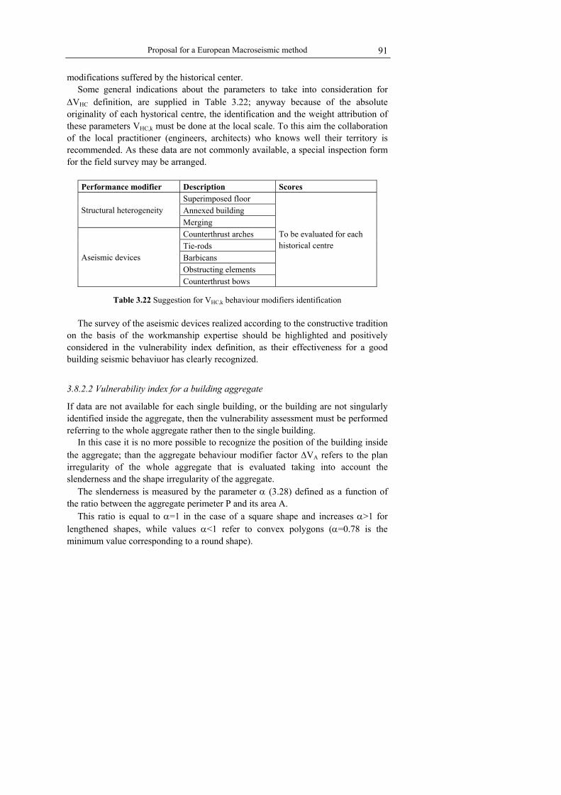
Proposal for a European Macroseismic method
91
modifications suffered by the historical center. Some general indications about the parameters to take into consideration for
∆VHC definition, are supplied in Table 3.22; anyway because of the absolute originality of each hystorical centre, the identification and the weight attribution of these parameters VHC,k must be done at the local scale. To this aim the collaboration of the local practitioner (engineers, architects) who knows well their territory is recommended. As these data are not commonly available, a special inspection form for the field survey may be arranged.
Performance modifier Description Scores
Superimposed floor Annexed building Structural heterogeneity Merging Counterthrust arches Tie-rods Barbicans Obstructing elements
Aseismic devices
Counterthrust bows
To be evaluated for each historical centre
Table 3.22 Suggestion for VHC,k behaviour modifiers identification The survey of the aseismic devices realized according to the constructive tradition
on the basis of the workmanship expertise should be highlighted and positively considered in the vulnerability index definition, as their effectiveness for a good building seismic behaviuor has clearly recognized.
3.8.2.2 Vulnerability index for a building aggregate
If data are not available for each single building, or the building are not singularly identified inside the aggregate, then the vulnerability assessment must be performed referring to the whole aggregate rather then to the single building.
In this case it is no more possible to recognize the position of the building inside the aggregate; than the aggregate behaviour modifier factor ∆VA refers to the plan irregularity of the whole aggregate that is evaluated taking into account the slenderness and the shape irregularity of the aggregate.
The slenderness is measured by the parameter α (3.28) defined as a function of the ratio between the aggregate perimeter P and its area A.
This ratio is equal to α=1 in the case of a square shape and increases α>1 for lengthened shapes, while values α<1 refer to convex polygons (α=0.78 is the minimum value corresponding to a round shape).
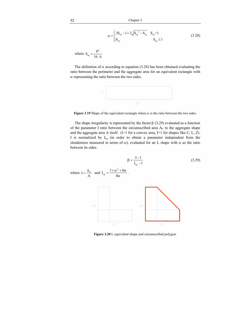
Chapter 3
92
2
eq eq eq eq
eq eq
2S 1 2 S S S >1
S S 1
− + −α = ≤
(3.28)
where 2
eqPS
16 A=
⋅
The definition of α according to equation (3.28) has been obtained evaluating the
ratio between the perimeter and the aggregate area for an equivalent rectangle with α representing the ratio between the two sides.
Figure 3.19 Shape of the equivalent rectangle where α is the ratio between the two sides. The shape irregularity is represented by the factor β (3.29) evaluated as a function
of the parameter I ratio between the circumscribed area AC to the aggregate shape and the aggregate area A itself. (I=1 for a convex area, I>1 for shapes like C, L, Z). I is normalized by Ieq (in order to obtain a parameter independent from the slenderness measured in terms of α), evaluated for an L shape with α as the ratio between its sides.
eq
I 1I 1
−β =
− (3.29)
where CAI
A= and
2
eq1 6I
8+ α + α
=α
.
Figure 3.20 L equivalent-shape and circumscribed polygon.

Proposal for a European Macroseismic method
93
∆VA can be attributed depending on the combination of values assumed by α and β parameters (Table 3.23).
Performance modifier Scores
0<β<0.3 0.3<β<0.5 0.5<β<1.5
0<α<3 0 0.02 0.04
3<α<5 0.02 0.04 0.06 Aggregate plan irregularity
α>5 0.04 0.06 0.08
Table 3.23 Values for the aggregate behaviour modifier factor ∆VA.
Beyond the plan irregularity, ∆VA behaviour factor should take into account the
interaction between adjacent buildings. When data are not available for each single building, it is possible to hypothesize a contribution in this sense referring to the statistical distribution of the building height in the historical centres.
Large scatter of this distribution have to be penalized as symptomatic of wide potentiality for different height adjacent building.
The historical centre behaviour modifier factor ∆VHC for the whole aggregate can be evaluated by a weight average of the VHC,k scores considering the percentage of buildings r k characterized by a certain VHC,k performance modifier. HC k HC,k
k
V r V∆ = ∑ (3.30)
3.9 THE UNCERTAINTY AFFECTING THE DAMAGE EVALUATION
The computation of the final vulnerability index V allows estimating a mean damage grade µD for a forecasted intensity scenario (3.11); coherently with the definition of the proposed method, µD values are distributed according to a beta probability density function (3.4).
In Table 3.24 the building typologies defined by EMS-98 scale are grouped depending on the width of the vulnerability index possibility range (difference between the lower Vmin and the upper bound Vmax).
It is worth noting that this range is different depending on the typology and that for buildings is higher on respect to vulnerability classes, for the reasons already mentioned in Par. 3.3. The same table shows two cases of possibility range reduced because of the application of the filter factor (Par. 3.4), to be employed when a deeper knowledge is achieved about the building stock.

Chapter 3
94
Classification of the Building System VMin - VMax
Vulnerability classes A, B, C, D, E, F 0.24
M1, M2, M3 0.4
M4, M5, M6, M7, RC4, RC5, RC6 0.56 Building Typologies
RC1, RC2, RC3, S, W 0.72
Existing data base (∆Vf=0.08) 0.24
Specific survey (∆Vf=0.04) 0.12
Table 3.24 Width of the vulnerability index possibility range for vulnerability classes and for
building typologies.
The use of a beta distribution allows to differently characterizing the scatter around the mean value. It has been possible to quantify this scatter depending on the amount of the cognitive uncertainty, by the use of a fuzzy random approach.
It is demonstrated (Ayyub and Chao 1998) that, considering a probabilistically distributed random variable with σ as its standard deviation, and assuming that the random variable X has a cognitive uncertainty in its mean value µ described by a membership function χ, the variance of the fuzzy-random variable is:
2 2 2
P Fσ = σ +σ (3.31)
where σP2 is the variance of the probabilistic distribution (the beta distribution in
this work) and σF2 is the variance of the membership function. σP
2 represents the
variability in the damage assessment while σF2 represents the cognitive uncertainty
in the mean damage µD evaluation due to be cognitive uncertainty in the vulnerability index definition.
It can be assumed that, considering a vulnerability class, the overall variance σ2 in formula (3.31) is known, as observed damage distributions on vulnerability classes have been well approximated by the use of a binomial distribution (Braga et al. 1982). From this assumption it is possible to evaluate the variance of the probabilistic distribution around each mean value:
2 2 2
P Fσ = σ −σ (3.32)
Once σP2 has been evaluated, the overall variance σ2 that describes the total
vriability of damage distributions can be obtained from (3.31) for the different cases of cognitive uncertainties presented in Table 3.24.

Proposal for a European Macroseismic method
95
3.9.1 Evaluation of the variance for mean damage membership functions
To exemplify how the variance of a membership function can be evaluated, let assume that the cognitive uncertainty in the mean value µ of a random variable X is described by a triangular fuzzy number (Figure 3.21) χ(µ) = [a,b,c] where a and c are the lower and the upper possible µ values for which the triangular membership function is χ=0, and b is the µ value corresponding to the highest degree of plausibility χ=1.
( )
ah a b
b a
ch b c
c b
µ −≤ µ ≤
−χ µ =
− µ≤ µ <
−
(3.33)
The function χ(µ) can be viewed as the probability density function for the
random variable. The mean value E[µ] and the variance Var[µ] for a the probability density function are by definition:
[ ]c
a
E ( ) d mµ = χ µ µ µ =∫ (3.34)
[ ] ( )c
2 2 2
a
Var E m ( ) d mµ = µ − = χ µ µ µ − ∫ (3.35)
Moreover as a probability density function χ(µ) it needs to satisfy the condition
that the integral from −∞ to +∞ must be equal to 1.
( )c
a
1( )d ( )d h c a 12
+∞
−∞
χ µ µ = χ µ µ = − =∫ ∫ (3.36)
Enforcing this condition, the height of the triangle membership function results:
( )2h
c a=
− (3.37)
Thus from equation (3.33) and (3.37) considering the definition provided for the
mean value (3.34) and the for the variance (3.35), E[µ] and Var[µ] for the considered triangular Membership Function χ(µ) = [a,b,c] result:

Chapter 3
96
[ ] a b cE
3+ +
µ = (3.38)
[ ]2 2 2a b c ab bc ac
Var18
+ + − − −µ = (3.39)
0
0.05
0.1
0.15
0.2
0.25
0.3
0.35
0.4
0.45
0.5
0 1.5 3 4.5 6
X
0
0.2
0.4
0.6
0.8
1
0 0.5 1 1.5 2 2.5 3 3.5 4 4.5 5 5.5 6
µ
χ(µ)
a
h
b c
Figure 3.21 Random distribution for the random variable X and Fuzzy distribution for its mean value µ.
In the hypothesis of a Membership Function symmetrical on respects to the
ordinate axis, formulas for the evaluation of mean and variance are evaluated in function of an only one parameter also for shapes different from the triangular.
In the hypothesis of a triangular membership function with b=0 and the upper and lower bounds corresponding to -c and c respectively χ(µ)=[-c,0,c], the variance can be evaluated as:
[ ]2c
Var6
µ = (3.40)

Proposal for a European Macroseismic method
97
For a trapezium Membership Function ( ) c cc, , ,c3 3
χ µ = − − the variance results:
[ ] 25Var c
27µ = (3.41)
µ
χ(µ)
c µ
χ(µ)
c
Figure 3.22 Triangular and trapezium membership function symmetrical on respects to the
ordinate axis. In order to allow an easier evaluation of the fuzzy variance σF
2 the hypothesis to describe the cognitive uncertainty on the mean damage grade µD by a symmetrical trapezium membership is suggested. Upper and lower values of this trapezium membership are µD(VMax,I) and µD(VMin,I) corresponding respectively to VMax and VMin according to formula (3.11), for a given macroseismic intensity I (Figure 3.23).
µD(VMax, I+0.5)
µD(VMax, I)
µD(VMin, I-0.5)
µD(VMin, I)
0
1
2
3
4
5
5 5.5 6 6.5 7 7.5 8 8.5 9 9.5 10 10.5 11 11.5 12EMS 98 Intensity
Mea
n D
amag
e G
rade
µD
V Max
V
V Min
Figure 3.23 Upper and lower values of the mean damage grade membership function. The c parameter to be substituted in formula (3.41) in order to evaluate the

Chapter 3
98
variance σF2 = Var[ µ] of the resulting mean damage membership function is:
( ) ( )D Max D MinV , I V , I
c2
µ −µ= (3.42)
In Figure 3.24 the fuzzy variance σF
2 is represented depending on the mean damage grade µD for the vulnerability classes and building typologies listed in Table 3.24.
0
0.1
0.2
0.3
0.4
0.5
0.6
0.7
0.8
0.9
1
0 1 2 3 4 5
Mean Damage Grade µD
Fuzz
y V
aria
nce
BT (M1, M2, M3)
BT (M4, M5, M6, M7, RC4, RC5,RC6)
BT ( RC1, RC2,RC3, S, W)
VC
BT (Specific survey)
Figure 3.24 Fuzzy variance for vulnerability classes and building typologies.
3.9.2 Evaluation of the probabilistic variance around the mean damage
Once the variance σF2 has been evaluated for a vulnerability class according to
(3.41), it is possible to determine the variability σP2 of the mean damage grade µD,
from formula (3.32). This can be done making reference to vulnerability classes. In this case, the
overall variance (total variability of the damage distribution) σ2 is assumed to be well approximated by the variance of a binomial distribution (3.3). In Figure 3.25 binomial distribution variance has been drawn as a function of the mean damage grade µD. It can be noticed how it is well approximated by the variance of the beta distribution assuming the parameter t equal to 7 (t=7). The evaluation of the variance for the discrete form of the beta distribution employed in the proposed method has been performed according to the definition provided by the probability theory:
( ) ( )2
xVar[X] x x f x dx= −∑ (3.43)
The resulting σP2 is well approximated by the variance of a beta distribution with
the parameter t equal to 8 (t = 8).

Proposal for a European Macroseismic method
99
0
0.2
0.4
0.6
0.8
1
1.2
1.4
0 0.5 1 1.5 2 2.5 3 3.5 4 4.5 5Mean damage grade
Var
ianc
e
Binomial Distribution Variance
Beta Distribution (t = 6.75) Variance
Beta Distribution (t = 7) Variance
Fuzzy Variance for VC
Probabilistic Variance
Beta Distribution (t = 8) Variance
Fuzzy Variance for VC (Intensity range)
Probabilistic Variance (No Intensityvariability)B t Di t ib ti (t 9 5) V i
Figure 3.25 Probabilistic variance σP
2 resulting from the difference between the binomial distribution variance σ2 and the vulnerability class fuzzy variance σF
2. Making reference to the evaluated σP
2, the total variance σ2 affecting damage
distributions for the different cases of cognitive uncertainty in Table 3.24 has been evaluated according to (3.31). Table 3.25 provides the t values corresponding to the total estimated variances σ2.
Classification of the building system t Vulnerability classes 7
M1, M2, M3 6 M4, M5, M6, M7, RC4, RC5, RC6 5
RC1, RC2, RC3, S, W 4.5Existing data base ∆Vf=0.08 7
Building Typology
Specific survey ∆Vf=0.04 8
Table 3.25 Values of the t parameter for distributions including the uncertainty in the hazard
description. As they have been obtained from observed damage distribution, the scatters
provided in Table 3.25 (in terms of t parameters) are all inclusive also in terms of the uncertainty affecting the hazard assessment.
In the following are also provided values for t parameter that allow obtaining damage distributions non inclusive of the uncertainty affecting the hazard; they have to be employed when the hazard uncertainties are provided together with the hazard description and have to be differently combined with others uncertainty sources. In this case, the σP
2 is as well evaluated according to (3.32) but putting out from the overall variance σ the variability that can affect on average the hazard assessment.

Chapter 3
100
Considering that an eventual uncertainty around an intensity value could be evaluated in terms of one intensity degree (Figure 3.23 dotted lines), the fuzzy variance is obtained σF
2 =Var[µ] computing the c parameter to be substituted in (3.41) as:
( ) ( )D Max D MinV , I 0.5 V , I 0.5
c2
µ + −µ −= (3.44)
The resulting σP
2 is less scattered than the one previously determined and it is
well approximated by the variance of a beta distribution with the parameter t equal to 9.5 (t = 9.5).
Table 3.26 provides t values corresponding to the total estimated variances σ2 for the different cases of cognitive uncertainty in Table 3.24. It is worth noting, once again, that the resulting distributions are less scattered than the ones provided in Table 3.25 as they do not include hazard uncertainties.
Classification of the Building System t Vulnerability classes 8.5
M1, M2, M3 7 M4, M5, M6, M7, RC4, RC5, RC6 6 RC1, RC2, RC3, S, W 5 Existing data base (∆Vf=0.08) 8.5
Building Typologies
Specific survey (∆Vf=0.04) 9.5
Table 3.26 Values of the t parameter for distributions non including the uncertainty in the hazard description.
3.10. DAMAGE, LOSS AND CONSEQUENCE DISTRIBUTIONS AND FRAGILITY CURVES FOR THE MACROSEIMIC APPROACH
The physical damage suffered by buildings because of an earthquake is only a small part of the total amount of the induced losses, but it has a key role in the loss and consequences evaluation as can be considered the root cause of many other losses. In concept, at least, once the physical damage distribution is available, consequences on buildings, people and economical losses can be estimated empirically by the use of correlations based on data observed after past earthquake.
According to the macroseismic method, once the expected mean damage grade is known µD (3.11) and the most reliable scatter for the distribution has been chosen (t parameter in Table 3.25 and Table 3.26), the evaluation of the damage distributions is a straightforward operation. Indeed the bounds of the distribution are fixed a = 0,

Proposal for a European Macroseismic method
101
b = 6 and the r parameter is obtained as a function of the parameter t and of the mean damage grade µD (3.10).
The fragility curve defining the probability of reaching or exceeding each damage grade Dk (k = 0÷5) are obtained directly from the beta cumulative density function:
[ ] ( )kD 1 P kP β= − (3.45)
Building physical damage distributions are obtained evaluating the probability pk
associated with each damage grade Dk (k = 0÷ 5) discretizing the beta cumulative density function or directly from the fragility curves:
( ) ( ) [ ]k k k 1p P k 1 P k D D = P Pβ β β β +
= + − − (3.46)
0
0.2
0.4
0.6
0.8
1
5 6 7 8 9 10 11 12 EMS-98 Intensity
Pk
D1
D2
D3
D4
D5
Figure 3.26 Macroseismic method damage fragility curves for a M4 (V=0.62, Q=2.3) building typology and corresponding histograms of damage distributions for I=9.
All mathematical programs allow evaluating the beta function once its parameters
are defined. Excel programme provides directly the beta cumulative density function as: ( )P x Distrib.beta(x, , , a, b)β = α β (3.47)
Where α=r and β=t – r on respect to the definition provided for the beta
cumulative density function in this work (3.4). Making reference to loss and consequence models presented in Par. 2.4,
macroseismic method allows immediately drawing fragility curves representing the occurrence probability of certain consequences to buildings, people or of certain economical losses.

Chapter 3
102
In particular, once physical damage fragility curves or damage probability distributions are evaluated respectively according to (3.45) and (3.46), fragility curves for uninhabitable dwelling (Ud) can be drawn making reference to equation (2.25) and to the rates wUd,k portrayed in Table (2.20) (as explained in Par. 2.4.1). In particular reference has been made to the model proposed by HAZUS (1999) for single family dwellings (SFD) and for single family dwellings (MFD) and to the model proposed by (Bramerini et al. 1995) referred as SSN.
Figure 3.27 shows uninhabitable dwelling fragility curves for M5 masonry building typology (Unreinforced Masonry-old bricks) where t=5 has been employed for the description of the damage distribution scatter according to Table 3.25.
Unreinforced Masonry
0
10
20
30
40
50
60
70
80
90
100
5 6 7 8 9 10 11 12 EMS98 - Macroseismic Intensity
% U
nfit
for u
se b
uild
ing
Hazus MFD t=5
Hazus SFD t=5
SSN t=5
Figure 3.27 Ud fragility curves for M5 typology (V=0.74, t=5).
It can be noticed how the SSN Italian proposal, valid indifferently for single and multiple family dwellings, lays in the middle between a superior and an inferior bound represented respectively by MFD and SFD HAZUS (1999) proposal. The fragility curves evaluated according to SSN proposal has been then drawn for different values of the parameter t in order to notice how a different scatter in the physical damage distribution can affect the consequences estimations in terms of uninhabitable dwelling (Figure 3.28).

Proposal for a European Macroseismic method
103
Unreinforced Masonry
0
10
20
30
40
50
60
70
80
90
100
5 6 7 8 9 10 11 12 EMS98 - Macroseismic Intensity
% U
nfit
for u
se b
uild
ing
SSN t=5
SSN t=6
SSN t=9.5
Figure 3.28 SSN Ud fragility curve for M5 typology and different values for t parameter. In particular in Figure 3.29, depending on the mean damage µD, the percentage
differences resulting in including (t=5) or not including (t=6) the hazard uncertainty and the differences in considering the two extreme situations in Table 3.26 for the cognitive uncertainty (t=5; t=9.5) are shown. In the first case a maximum difference of 2% is reached, in the second case a maximum difference of 4% is observed.
-6
-4
-2
0
2
4
6
0 0.5 1 1.5 2 2.5 3 3.5 4 4.5 5
Mean Damage Grade
Diff
% U
fu e
stim
atio
n fo
r diff
eren
t t
SSN t=5 - t=9.5
SSN t=5 - t=6
Figure 3.29 Percentage differences in the Ud building estimation employing different t values In the same way, fragility curve for casualty estimations have been evaluated on
respect to the assumed injury severity scale (Table 2.23) starting from macroseismic damage distributions or fragility curves and making reference to what explained in Par. 2.4.2. It is worth remembering that according to SSN proposal (Bramerini et al. 1995) a unique evaluation can be achieved for the sum of severity S3 and S4 (2.31) while HAUS (1999) allows the evaluation of casualty fragility curves for each

Chapter 3
104
severity degree (Table 2.24). For the definition of S4 casualty fragility curves according to Coburn and Spence (1992) proposal, it must be taken into account that the injury distribution at collapse and post collapse is provided for masonry building for discrete values of the macroseimic intensity (Table 2.25). In order to draw fragility curves a continuous correlation between collapse rates and intensities has to be introduced on the basis of the values supplied in Table 2.28. In particular Figure 3.30 shows the one assumed for the post-collapse rates that can be considered to provide the sum of severity S3 and S4.
Unreinforced Masonry Building
0
5
10
15
20
25
30
35
40
45
50
5 6 7 8 9 10 11 12
EMS98 Macroseismic Intensity
% D
eath
Rat
e
Figure 3.30 Death rate and intensity correlation for URM building.
( ) [ ]( ) [ ]( ) [ ]
[ ]
3 4
5
5S S
5
5
0.075I - 0.42 P D 6 I< 8
0.18I - 1.26 P D 8 I< 9
0.06I - 1.18 P D 9 I< 10
0.42P D I 10
P
β
β+
β
β
≤
≤=
≤ ≥
(3.48)
Figure 3.31 shows casualty fragility curves for unreiforced masonry building and
for the different proposal analysed. In particular, for Coburn and Spence (1992) proposal reference has been made to the post collapse rates (Table 2.28) and for HAZUS (1999) proposal the sum of different injury severity levels (S3+S4) has been considered.

Proposal for a European Macroseismic method
105
Unreinforced Masonry Building
0
5
10
15
20
25
30
35
40
45
50
7 7.5 8 8.5 9 9.5 10 10.5 11 11.5 12EMS98 Macroseismic Intensity
% D
ead
and
Seve
rly In
jure
d Pe
ople HAZUS S3+S4
SSN Dead & SeverlyInjured
COBURN & SPENCE S4 Post Collapse
Figure 3.31 Casualty fragility curve for unreinforced masonry building (V=0.74 , t=5). Once again the Italian proposal lies in the middle of the other two. The reason for
the huge scatter between these proposals may be found in the different origin of the data processed in order to obtain these correlations.
Finally, Damage Factor fragility curves (usually referred as Mean Damage Ratio MDR fragility curves) have been drawn for the ATC13 (1987), SSN (Bramerini et al. 1995) and HAZUS (1999) proposal (Table 2.27) and their trend is portrayed in Figure 3.32 for unreinforced masonry building typology.
Unreinforced Masonry Building
0
10
20
30
40
50
60
70
80
90
100
5 6 7 8 9 10 11 12EMS-98 Macroseismic Intensity
% M
DR
ATC13*
HAZUS
SSN
Figure 3.32 MDR fragility curve for unreinforced masonry building (V=0.74 t=5).

Chapter 3
106
3.11 VALIDATION OF THE METHODOLOGY
3.11.1 Comparison with observed damage data
A good agreement has been observed between the proposed Macroseismic Method for masonry structures and observed damage data (Table 3.27), data elaborated from damage observed (Table 3.28) and an observed vulnerability method (Oliveira e Mendes Victor, 1984). The comparison has been performed, in terms of vulnerability curves, considering carefully the relation between the macroseismic scales to which data refer and EMS-98 scale and between data damage description and the EMS-98 discrete 5 grade damage scale in order to represent the available data in a IEMS98-µD plot.
For each masonry typology considered by the classification system, Macroseimic Vulnerability curves drawn for the most probable value of the specific building V0
and the uncertainty bound around it V+ V- (Table 3.4) have shown to contains these
data. Label Earthquake Intensity DS Reference Banja Luka ’69 Banja Luka 27.10.1969
(Bosnia-Herzegovina) MSK-64 5DG Stojkovic, 1978
Gediz ’70 Gediz (Turchia) 28.03.1970 MM (IX) 3 DG Arioglu et Anadol, 1973 Bingol ’71 Bingol (Turchia) 22.05.1971 MM (VIII) 4 DG Karaesmen, 1973 Burdur ’71 Burdur (Turchia) 12.05.1971 MM VIII 3 DG Arioglu et Anadol, 1973 Lice ’75 Lice (Turchia) 06.09.1975 MM (XI) 3 DG Arioglu et Anadol, 1977 Bucarest ’77 Bucarest 04.03.1977
(Romania) EMS-98 5 DG Balan et al, 1982
Irpinia ’80 Irpinia (Italia) 23.11.1980 MSK-76 3 DG Braga et al. 1982 Mont Chenoua ’89 Mont Chenoua 29.10.1989
(Algeria) MM (VIII) 5 DG Farsi et Belazougui, 1992
Luzon ’90 Luzon (Filippine) 16.07.1990 MM (VIII) 3DG Otani, 1999 Erzincan ’92 Ernzican (Turchia) 13.03.1992 MM (IX) 3DG Otani, 1999 Hyogo-ken Nambu ’95
Hyogo-ken Nambu (Kobe- Giappone) 17.01.1995
JMA(VI-VII
5DG Okada et al, 2000
Table 3.27 Available observed damage data.
Label Earthquake Intensity DS Reference Salonicco ’78 Salonicco (Grecia) 20.06.1978 EMS-98 VI-VII 4DG Kappos et al, 1995 Aegion ’95 Aegion (Grecia) 15.06.1995 EMS-98 VII 4DG Kappos et al, 1995
Table 3.28 Data elaborated from damage observed.

Proposal for a European Macroseismic method
107
0
1
2
3
4
5
5 6 7 8 9 10 11 12 EMS-98
µ D
M1-M1M1+Bingol '71Lice '75Irpinia '80
0
1
2
3
4
5
5 6 7 8 9 10 11 12EMS-98
µ D
M2-M2M2+Burdur '71Mont Chenoua '89
0
1
2
3
4
5
5 6 7 8 9 10 11 12 EMS-98
µ D
M3-M3M3+LisbonBanja Luca '69Bingol '71Gediz '70Burdur '71Thessaloniki '78Irpinia '80Aegion '95
0
1
2
3
4
5
5 6 7 8 9 10 11 12EMS-98
µ D
M4-M4M4+Lisbon
0
1
2
3
4
5
5 6 7 8 9 10 11 12 EMS-98
µ D
M5.w-M5.wM5.w+LisbonBanja Luca'69Bucharest '77, 1Bucharest '77, 2Bucharest '77, 3Bucharest '77, 4Irpinia '80
0
1
2
3
4
5
5 6 7 8 9 10 11 12EMS-98
µ D
M5.sm-M5.smM5.sm+Irpinia '80
0
1
2
3
4
5
5 6 7 8 9 10 11 12 EMS-98
µ D
M6-M6M6Thessaloniki '78Irpinia '80Aegion '95
0
1
2
3
4
5
5 6 7 8 9 10 11 12EMS-98
µ D
M7-M7M7+Lisbon
Figure 3. 33 Vulnerability curves from the Macroseismic method for different masonry building typologies and comparison with observed damage data.
3.11.2 Comparison with Coburn and Spence PSI vulnerability method
The parameterleless scale of seismic intensity (PSI scale) is a scale of earthquake strong motion damage measured by the performance of samples of buildings of standard types. It is based on the observation that, although assigned intensity in

Chapter 3
108
different surveys varies widely even with the same level of loss, the relative proportions of a sample of buildings of any type in different damage states are fairly constant, and so are relative loss levels of different building classes surveyed at the same location. The PSI scale is based on the proportion of brick masonry buildings damaged at or above level D3; it is assumed that this proportion is normally distributed with respect to the ground motion scale. The PSI parameter ψ is defined so that 50% of the sample is damaged at level D3 or above when ψ=10 and the standard deviation is σ = 2.5. Using this curve as a basis, the curves for other damage levels are defined from the relative performance of buildings in a large number of surveys. Likewise, vulnerability curves for other building types have been derived from their performance relative to brick building in the surveys.
Since the vulnerability curves are of cumulative normal or Gaussian form, the proportion of building damaged to any particular damage or greater is given by the standard distribution function.
The cumulative distribution function, providing the percentage (0÷1) of the building stock D damaged, is defined as:
21 1 MD exp
22
ψ
−∞
ψ − = − σπσ ∫ (3.49)
where M and σ are respectively, the mean and the standard deviation σ of the
normal distribution and ψ is the intensity. Values of the Gaussian distribution parameters M and σ for a range of common
building types and damage states have been derived from the damage data in the Martin Centre damage database.
From what shown in Coburn and Spence (2002) it has been deduced that the PSI intensity ψ, relates to the EMS-98 macroseismic intensity I according to the following linear correlation:
I 0.54 3.25= ⋅ψ + (3.50)
Table 3.29 shows the correspondence found between the classification system considered by PSI scale vulnerability approach, and the one proposed in the framework of these work (Table 2.5). For the same typologies the parameters defining the mechanical approach are provided together with the ones defining PSI curves (Table 3.30). PSI values are derived from observed data with a different level of confidence (also reported in Table 3.30).
A very good matching between the two curves have been found employing a parameter t=4 for the description of damage distribution scatter according to the macroseismic method (Table 3.30). This means that the PSI scale methods provides more scattered results in comparison to the ones obtained employing the

Proposal for a European Macroseismic method
109
macroseimic approach (where higher values of t are employed).
Building typology classification PSI scale building classification M1 Rubble stone AR1 Rubble stone masonry M2 Adobe AA1 Adobe (earth brick) masonry M5 Unreinforced Masonry BB1 Brick masonry unreinforced M7 Reinforced Masonry DB1 Reinforced Unit Masonry RC1-PC RC frame – Pre Code CC1 RC frame, non seismic RC1-LC RC frame – Low Code DC2 RC frame, seismic design UBC2RC1-MC RC frame – Medium Code DC3 RC frame, seismic design UBC3RC1-HC RC frame – High Code DC4 RC frame, seismic design UBC4
Table 3.29 Matching between the proposed classification system and the PSI classification
system.
Macroseimic Method PSI scale Method V Q t D1 D2 D3 D4 D5 ConfidenceM1 0.87 2.3 4 AR1 3.2 5.9 8.2 9.8 11.7 High M2 0.84 2.3 4 AA1 3.9 6.6 8.9 10.5 12.4 Good M5 0.72 2.3 4 BB1 4.9 7.8 10 11.6 13.3 High M7 0.45 2.3 4 DB1 7.5 10.6 13 15 17 Good RC1-PC 0.64 2.3 4 CC1 7.9 10.3 11.3 12.9 14.1 High RC1-LC 0.56 2.3 4 DC2 8.8 10.5 12.5 14.1 15.2 Moderate RC1-MC 0.48 2.3 4 DC3 9.4 11.1 13.0 14.7 16.4 Moderate RC1-HC 0.32 2.3 4 DC4 10.6 12.4 14.7 17.0 18.8 Moderate
Table 3.30 Parameters defining macroseismic method and PSI method for the building
typologies considered in Table 3.29.
M1-Rubble Stone
0
0.1
0.2
0.3
0.4
0.5
0.6
0.7
0.8
0.9
1
5 6 7 8 9 10 11 12 EMS98 - Macroseismic Intensity
% o
f Bui
ldin
g D
amag
ed
D1- PSI MethodD2- PSI MethodD3- PSI MethodD4- PSI MethodD5- PSI MethodD1 MacroseismicD2 MacroseismicD3 MacroseismicD4 MacroseismicD5 Macroseismic
M2-Adobe
0
0.1
0.2
0.3
0.4
0.5
0.6
0.7
0.8
0.9
1
5 6 7 8 9 10 11 12 EMS98 - Macroseismic Intensity
% o
f Bui
ldin
g D
amag
ed
D1 PSI MethodD2 PSI MethodD3 PSI MethodD4 PSI MethodD5 PSI MethodD1 MacroseismicD2 MacroseismicD3 MacroseismicD4 MacroseismicD5 Macroseismic

Chapter 3
110
M5 - Unreinforced Masonry
0
0.1
0.2
0.3
0.4
0.5
0.6
0.7
0.8
0.9
1
5 6 7 8 9 10 11 12 EMS98 - Macroseismic Intensity
% o
f Bui
ldin
g D
amag
ed
D1 PSI MethodD2 PSI MethodD3 PSI MethodD4 PSI MethodD5 PSI MethodD1 MacroseismicD2 MacroseismicD3 MacroseismicD4 MacroseismicD5 Macroseismic
M7 - Reinforced Masonry
0
0.1
0.2
0.3
0.4
0.5
0.6
0.7
0.8
0.9
1
5 6 7 8 9 10 11 12 EMS98 - Macroseismic Intensity
% o
f Bui
ldin
g D
amag
ed
D1 PSI MethodD2 PSI MethodD3 PSI MethodD4 PSI MethodD4 PSI MethodD1 MacroseismicD2 MacroseismicD3 MacroseismicD4 MacroseismicD5 Macroseismic
Figure 3.34 Comparison between the EMS-98 damage fragility curves and PSI damage
fragility curves.
3.11.3 Calibration on respect to GNDT I & II level vulnerability method
In Italy two distinct methodologies have been traditionally used, referred to as GNDT I and II level and developed in the area of the activities of GNDT (National Group for Defence from Earthquakes) over the last twenty years.
The GNDT I level approach (Corsanego and Petrini 1994) can be classified as an observed vulnerability methods as it has been developed on the basis of damage effectively found following the strong seismic events that have hit the national territory (starting from November 1980 Irpinia earthquake) (Braga et al. 1982). The GNDT II (Benedetti and Petrini 1984, GNDT 1994) level approach can be defined
RC1_W ERD - RC frame, non seismic
0
0.1
0.2
0.3
0.4
0.5
0.6
0.7
0.8
0.9
1
5 6 7 8 9 10 11 12 EMS98 - Macroseismic Intensity
% o
f Bui
ldin
g D
amag
ed
D1 PSI MethodD2 PSI MethodD3 PSI MethodD4 PSI MethodD5 PSI MethodD=1 MacroseismicD=2 MacroseismicD=3 MacroseismicD=4 MacroseismicD=5 Macroseismic
RC1_L ERD - RC frame, seismic design UBC2
0
0.1
0.2
0.3
0.4
0.5
0.6
0.7
0.8
0.9
1
5 6 7 8 9 10 11 12 EMS98 - Macroseismic Intensity
% o
f Bui
ldin
g D
amag
ed
D1 PSI MethodD2 PSI MethodD3 PSI MethodD4 PSI MethodD5 PSI MethodD=1 MacroseismcD=2 MacroseismcD=3 MacroseismcD=4 MacroseismcD=5 Macroseismc
RC1_M ERD - RC frame, seismic design UBC3
0
0.1
0.2
0.3
0.4
0.5
0.6
0.7
0.8
0.9
1
5 6 7 8 9 10 11 12 EMS98 - Macroseismic Intensity
% o
f Bui
ldin
g D
amag
ed
D1 PSI MethodD2 PSI MethodD3 PSI MethodD4 PSI MethodD5 PSI MethodD=1 MacroseismicD=2 MacroseismicD=3 MacroseismicD=4 MacroseismicD=5 Macroseismic
RC1_H ERD - RC frame, seismic design UBC4
0
0.1
0.2
0.3
0.4
0.5
0.6
0.7
0.8
0.9
1
5 6 7 8 9 10 11 12 EMS98 - Macroseismic Intensity
% o
f Bui
ldin
g D
amag
ed
D1 PSI MethodD2 PSI MethodD3 PSI MethodD4 PSI MethodD5 PSI MethodD=1 MacroseismicD=5 MacroseismicD=3 MacroseismicD=4 MacroseismicD=5 Macroseismic

Proposal for a European Macroseismic method
111
as a semeiotic approach developed on the basis of expert-judgement. Some more information about these methods has been already included in Par 2.3.1.1. These methods have been considered throughout the years of their application as conceptually non comparable. As a matter of fact GNDT I level subdivides the analysed built-system into homogeneous subgroups, on the basis of the construction typology, and supplies for each one the statistical distribution of the expected damage. On the other hand, GNDT II level refers to each single building and identifies its vulnerability through an index (obtained from the score assigned to the characteristics of the different elements of the construction) and proposes a deterministic correlation between the seismic input and the expected damage.
Moreover, the hazard and the damage descriptions are different for the two methods. According to GNDT I level the earthquake is considered in terms of macroseismic intensity and the damage is described through qualitative levels, associated with the evidence of particular damaging states or of partial or total collapse. On the other hand GNDT II level represents the damage in economic terms, and the hazard in terms of PGA.
In reality these differences are not substantial. The II level evaluation, even if carried out on each single building, represents an average value of the response of the buildings with those characteristics (and it is known that the confidence intervals of these curves are very wide). Furthermore, the choice of the PGA as a seismic parameter is connected with the desire to use a continuous parameter (different from intensity) and of clearer mechanical significance, but these curves have been originally derived from experimental observation data in intensity and subsequently translated through Guagenti and Petrini (1989) correlation (2.2). Finally the representation of the damage in economic terms has been obtained appling the SSN physical damage-damage factor correlation (Table 2.29).
These considerations have lead to the representation of GNDT I level vulnerability curves and of GNDT II level fragility curves on a common I-µD diagram. Furthermore they have suggested the idea of a hybrid semeiotic-typological approach that is at the basis of the proposed Macroseismic approach.
0
0.5
1
1.5
2
2.5
3
3.5
4
4.5
5
5 5.5 6 6.5 7 7.5 8 8.5 9 9.5 10 EMS-98 Intensity
µD
GNDT II Level Iv=80GNDT II Level Iv=60GNDT II Level Iv=40GNDT II Level Iv=20GNDT I Level - Class AGNDT I Level - Class BGNDT I Level - Class C
Figure 3.35 GNDT I and II level comparison on a I-µD diagram.

Chapter 3
112
Figure 3.35 shows this comparison, from which it comes out just how the trend is qualitatively analogous, apart from the end zones of the curves of II level, which show a more abrupt trend. This difference is simply linked to the fact that, for the sake of simplicity, the curves of II level are defined by a tri-linear trend; the real behavior is certainly different in that a building starts to be damaged, even if in a reduced way, already with small earthquakes and, similarly, only with great difficulty does it collapse completely.
GNDT I and II level have been moreover compared with EMS-98 curves. Figure 3.36 (left side) shows the comparison with GNDT I level approach, from which it clearly emerges how the trend of GNDT and EMS-98 curves is analogous and how a good correspondence exists between the three classes of Irpinia DPM and the EMS-98 first three vulnerability classes (A÷C). It should be said that the Irpinian DPM make reference to the MSK-76 macroseismic scale; in the document that defines the EMS-98 scale it is stated that there is substantial equality between the scales, even if conceptually a direct comparison is not possible.
0
0.5
1
1.5
2
2.5
3
3.5
4
4.5
5
5 5.5 6 6.5 7 7.5 8 8.5 9 9.5 10 EMS-98 Intensity
µD
GNDT I Level - Class AGNDT I Level - Class BGNDT I Level - Class CEMS-98 Class A+0.08 [V=0.98]EMS-98 Class B+0.08 [V=0.82]EMS-98 Class C+0.08 [V=0.66]
0
0.5
1
1.5
2
2.5
3
3.5
4
4.5
5
5 5.5 6 6.5 7 7.5 8 8.5 9 9.5 10 EMS-98 Intensity
µD
EMS-98 Class A [V=0.90]EMS-98 Class B [V=0.74]EMS-98 Class C [V=0.58]GNDT II Level Iv=60GNDT II Level Iv=40GNDT II Level Iv=20
Figure 3.36 EMS-98 comparison with GNDT I level approach (on the left) and GNDT II
level approach (on the right). Figure 3.36 (right side) shows the comparison between Macroseismic Method
vulnerability curves and GNDT II level method curves. The observed matching between EMS-98 vulnerability classes and the GNDT II level curve vulnerability index (Iv) values is portrayed in Table 3.31.
EMS-98 class A B C D E
Vulnerability index IV 60 40 20 0 -20
Table 3.31 EMS-98 vulnerability classes and corresponding GNDT II vulnerability indexes. On the basis of this comparison, the following correlation has been established
between the GNDT II level vulnerability index Iv and the proposed Macroseimsic Method V vulnerability index: VI 156.25V 76.25= − (3.51)

A Mechanical based method for European building typologies 113
CHAPTER 4
A MECHANICAL BASED METHOD FOR EUROPEAN BUILDING
TYPOLOGIES
4.1 CAPACITY CURVES FOR CAPACITY SPECTRUM VULNERABILITY METHODS
The most recent trend in the field of vulnerability evaluation for risk analysis lead to operate with simplified mechanical models essentially based on the Capacity Spectrum Method (Freeman 1998, HAZUS 1999). This method permits evaluating the expected seismic performance of a structure, assumed as an equivalent non linear single degree of freedom system (s.d.o.f), by intersecting, in spectral coordinates (Sd, Sa), its seismic capacity curve with the seismic demand, described by the Acceleration-Displacement Response Spectra (ADRS), adequately reduced in order to take into account the inelastic behaviour. The intersection point, between seismic capacity and seismic demand curve, is referred as performance point (p.p).
Capacity curves aim to represent the first mode response of the building assuming that it is the predominant mode of the buildings vibration and that it primarily controls the damage genesis and progress. Capacity curves are usually drawn implementing “pushover” analyses that lead to the evaluation of pushover curves, representing the building lateral load resistance V (static equivalent base shear) versus its characteristic lateral displacement ∆R (peak displacement of the building roof). Capacity curves are derived from pushover curves identifying on them two characteristic control points: the yield capacity YC and the ultimate capacity UC (Figure 4.1). The yield capacity YC represents the lateral load resistance strength of the building before structural system has developed non-linear response. The ultimate capacity UC is defined as the maximum strength of the building when the global structural system has reached a fully plastic state. Up to the yield point, the building capacity is assumed to be linear with stiffness based on an estimate of the true period of the building. From the yield point to the ultimate point, the capacity curve transitions in slope from an essentially elastic state to a fully plastic state. Beyond the ultimate point buildings are assumed capable of deforming without loss of stability, but their structural system provides no additional resistance to lateral earthquake force.

114 Chapter 4
Ultimate Capacity (UC)
Yield Capacity (YC)
Design Capacity (DC)
∆R ∆u ∆y∆d λ∆y
Vd
Vy
Vu
V
Figure 4.1 Bilinear capacity curve derived from a pushover curve. In order to assure a direct comparison between the building capacity and the
demand spectrum as well as to facilitate the determination of the performance point (p.p.), the base shear V has to be converted into spectral acceleration Sa and the roof displacement ∆R into spectral displacement Sd (Chopra and Goel 1999). The capacity curve of a model structure presented in AD format is termed Capacity Spectrum (Freeman 1975, Freeman 1998).
Conversion of capacity curve (V, ∆R) to capacity spectrum shall be accomplished by knowing modal properties that represent pushover response. For this, a single degree of freedom system (s.d.o.f) (Shibata and Sozen 1976) is used to represent a translational vibration mode of the structure.
In particular the modal properties to be known are the modal participation factor Γ (4.1) and the modal mass coefficient m for the first natural mode (4.2) respectively defined as:
i i2
i i
m
m
ΦΓ =
Φ∑∑
(4.1)
( )2
i i
2i i i
mm
m m
Φ=
Φ
∑∑ ∑
(4.2)
where mi is the story mass at level-I, Φi is the amplitude of the first mode at level-
i (the vector component describing the first mode shape at level–i), that is normalized to the roof displacement.
The conversion of any capacity curve points (Vi, ∆Ri) into the corresponding first mode spectral coordinates (Sai, Sdi) (4.3) is performed as a function of the modal

A Mechanical based method for European building typologies 115
participation factor Γ and of the modal mass coefficient m above defined (Vidic et al. 1994):
i
i
i
ia
Rd
R
VS
mM
S
=
∆=
Γφ
(4.3)
where M is the building dead weight plus likely live loads and φR is the roof level
amplitude of the first mode. To enable the estimation of an appropriate reduction of the spectral demand, a
bilinear form (blu line in Figure 4.1) is often used both for the capacity spectrum graphical and numerical representation.
4.2. SIMPLIFIED CAPACITY CURVES FOR BUILDINGS TYPOLOGIES
The capacity curve of a structure should be obtained by a pushover analysis, but in the case of a territorial vulnerability assessment, bilinear capacity curves can be defined in a simplified way.
Dealing with a building stock characterized by a typological building homogeneity and by consolidated seismic design codes (and rigorous legal system assuring their strict implementation), the estimation of the defining parameters can be performed making reference to the values prescribed by national seismic design codes and to the construction material standards. On the other hand, for non designed structures (i.e. the broad and wide diversified masonry building patrimony belonging to European regions) bilinear capacity curve can be derived taking into account the geometrical and the technological features characterizing on the average the typology (number of floors, code level, material strength, drift capacity, age, etc.) and hypothesizing a certain collapse mode.
Assuming a bilinear representation, Capacity Spectrum is completely identified in terms of yielding (dy, ay) and ultimate (du, au) points being dy the yield spectral displacement ay the yield spectral acceleration, du the ultimate spectral displacement and au the ultimate acceleration.
In the further hypothesis to neglect the hardening behavior, capacity curves can be completely defined by three parameters, the yield acceleration ay, the true fundamental period of the structure T and the structural ductility capacity µ.
As a matter of fact, the yielding displacement dy can be obtained as a function of the yielding acceleration ay, once the true period of the structure T is known:
2
y yTd a2
= π (4.4)

116 Chapter 4
And the ultimate displacement du can be evaluated once the building ductility capacity µ is provided:
u yd d= µ (4.5)
4.2.1 Capacity curves derived from seismic design codes
According to Kircher et al. (1997), for designed building, the yield YC and the ultimate UC control points (Figure 4.1) can be related to the design prescriptions as follow:
( )
y 2y s y 2
u y u y
VYC V C T
4
UC V V
,
,
= = γ ∆ = π
= = λ ∆ = λµ∆ (4.6)
where Cs is the point of significant yielding of design strength coefficient
(fraction of the building weight), T is the true elastic fundamental-mode period of building (in seconds), γ is the overstrength factor relating design strength to true yield strength, λ is the overstrength factor relating ultimate strength to yield strength, and µ is the ductility factor relating ultimate ∆u displacement to λ times the yield displacement.
According to (4.3) the conversion in terms of spectral coordinates of the two control points defined in (4.6) results as:
y y
u y
y yy a y d
u uu a u d
VYC a S d S
mM
VUC a S d S
mM
∆ = = = = = Γ
∆ = = = = = Γ
,
,
(4.7)
Therefore, making reference to the values prescribed by seismic design codes and
by construction material standards, a Code Based Approach (referred in the following as CBA) has been applied in order to draw, for designed reinforced concrete typologies, symplified capacity curves in terms of yielding acceleration ay, ductility capacity µ, and fundamental period T.
As a matter of fact, the building ductility capacity µ, and the fundamental period T parameters are usually defined by code requirements for different structural types. The yield acceleration ay can be derived as a function of the seismic code lateral-force design requirements, being aware that factors like redundancies and conservatism in design, and true strength of materials have to be considered rather than the nominal ones.

A Mechanical based method for European building typologies 117
The CBA approach has been developed, in the following, for two different codes and for different seismic zone locations, making reference to Italian territory. It goes without saying that the same procedure can be followed wanting to represent in terms of capacity curves the level of seismic protection achieved in different european countries and for different time of construction.
Table 4.1 shows, for istance, the seismic codes shear base formulations for different European countries (Milutinovic and Trendafiloski 2003) for a period ranging from 1974 to 1993. It is worth noticing that all the formulas consist of parameters relating to seismic zone, soil condition, building dynamic response, structural type and building importance.
Country Base shear coefficient
Zon
e Fa
ctor
Stan
dard
Bas
e-Sh
ear
Coe
ffic
ient
Dyn
amic
Fac
tor
Stru
ctur
al F
acto
r
Site
Coe
ffic
ient
O
ccup
ancy
Impo
rtan
ce
Fact
or
Oth
ers
Yea
r
Spain α β δ; [α=CR, β=B/T1/3] C β B δ R(1) 1974
France (*) α β δ α β δ 1982
Italy (*) C R ε β I; [C=(S-2)/100] C K S I 1990
Ex-Yugoslavia K0 Ks Kd Kp Ks Kd Kp
K0
1981
Greece α I B(T) n θ R/q α B(T) q θ I n(2) 1992
Romania (**) α ψ Ks βr Ks βr ψ α 1991
Bulgaria (*) C R Kc βi Kψ Kc βi R C 1987 (*) Lateral force coefficient method is used (**) Dynamic modal distribution factor method is used (1) Zone risk factor (2) Damping Coefficient factor
Table 4.1 Seismic code base shear formulation for different European countries.
4.2.1.1 DM96 Italian Seismic Code
Capacity curves have been derived from D.M. 16.1.96 (Ministry of Public Works Decree of January 16, 1996) referred in the following as DM96. The Code is direct to every construction placed in areas officially indicated as seismic according to n°64/74 (art.3) law, that subdivide Italy in four zones: zone I high seismicity, zone II medium seismicity, zone III low seismicity and zone IV where no seismic actions are considered.
According to DM96, a static analysis can be used for regular structures; these structures are considered to be subjected to a system of horizontal forces having the

118 Chapter 4
same direction chosen for the earthquake. The resultant of such forces is defined as: F C R I M= (4.8)
where C is the seismic intensity coefficient, R is the response coefficient in the
direction considered, I is the seismic protection coefficient and M is the total weight of seismic masses.
The seismic intensity coefficient C is defined as a function of the degree of seismicity S, differently provided for the three seismic zones considered:
S 2C100
−= (4.9)
where S=12 and C=0.1 for zone I, S=9 and C=0.07 for zone II and S=6 and
C=0.04 for zone III. The response coefficient R is a function of the fundamental period T, assuming a
value R=1 when T≤0.8 [s] and when the fundamental period T is not determined. The seismic protection coefficient is I=1 for ordinary buildings (buildings that are
not considered strategic for emergency questions or that are not particularly crowded).
To well approximate the seismic dynamic effects, two more coefficients are considered for the distribution of the resultant force (4.8) in plan and height. The horizontal force at the generic I-elevation Fi, for a certain direction, is defined as: i iF C R I M= ε β (4.10) where ε is the foundation factor, β is the structure factor and Mi is the weight to be used for seismic action at i-level.
The foundation factor is usually ε=1 being ε=1.3 only when the subsoil profile includes an alluvial surface layer with thickness varying between 5 and 20m, underlain by much stiffer materials, such as cohesive or rock soils.
The structure factor β is differently defined depending on the structural typology considered. Table (4.2) portrayts β values provided by DM96 for three reinforced concrete building typologies, whose description matches with reinforced concrete building typologies considered in this work (Table 2.5).
RC1 Frame structure in reinforced concrete β=1 RC2 Structure with bearing wall system β=1.4 RC3 Structure with frames stiffened by vertical elements carrying most of the
horizontal actions β=1.2
Table 4.2 DM96 structure factor β for reinforced concrete building typologies.

A Mechanical based method for European building typologies 119
Having defined the base shear as (4.10) and making reference to (4.3), the yielding spectral acceleration ay results: ya C R I= ε β (4.11)
It is worth noting that the modal mass coefficient m, contained in the definition of the yielding acceleration ay (4.3) has been neglected as it has been considered to be included in the definition of the structure factor β.
In order to draw capacity curve according to DM96, two further considerations have to be done for the final definition of ay. First of all, the forces check is performed in DM96 according to the ultimate limit state (U.L.S) resistance. For the U.L.S. checks the forces are evaluated making reference to a specific combination formula according to which the forces due to the conventional earthquake have to be multiplied for a coefficient γe =1.5.
Secondly, as previously stated, defining capacity curves from codes the true strength of materials has to be considered (rather than nominal the nominial one, as defined by standards for code designed and constructed buildings). DM 9.1.96 ( Ministry decree of January, 9, 1996 “Rules for the design, execution, inspection and strengthening of reinforced concrete, prestressed concrete and steel structures”) provides characteristic yield strength for two classes of ribbed steel (Fe B 38 K fyk=375 N/mm2, and Fe B 44 K fyk=430 N/mm2) and characteristic compressive strength for reinforced concrete fck. DM 9.1.96 establishes that the coefficients leading to the design strength are γm=1.6 for reinforced concrete and γm=1.15 for steel. According to DM 9.1.96 the characteristic strength (representing the 5% percentile) can be related to the strength median value by a coefficient α=0.7.
k mD
m m
f ff
α= =
γ γ (4.12)
Taking into account these two further aspects, the yielding acceleration ay
resulting from DM96 can be written as:
[ ] my Ea C R I
γ= γ ε β
α (4.13)
With regard to γm value to be used in (4.13), reference has been made to the one
prescribed by DM 9.1.96 for reinforced concrete compressive strength (γm=1.6). Thus considering that the reinforced concrete crisis is the prevalent failure mode and that steel is often characterized by a higher quality on respect to the one cerfied. This is moreover justified wanting to take into account the conservatism in design that, as shown after recent earthquakes (Freeman 2004), have lead properly code designed buildings, to survey major seismic actions.

120 Chapter 4
The expression provided by DM96 for the building fundamental period T evaluation (4.14) can not be employed because it requires the knowledge of the building typology withd B.
HT 0 1B
= . (4.14)
Therefore, for the evaluation of the elastic period of the structure T reference has
been made to the expression proposed by EC8 (CEN 2003) for buildings with heights up to 40m:
34
tT C H= (4.15)
where H is the height of the building from the foundation or from the top of a rigid basement and Ct coefficient is defined depending on the building typology: Ct= 0.085 for moment resistant space steel frames, Ct= 0,075 for moment resistant space concrete frames and for eccentrically braced steel frames, Ct= 0,05 for all the other structures.
With regard to the ductility capacity µ, DM96 does not provide any specific prescription. A value µ = 2.5 has been assumed, judged to be suitable for the ductility capacity representation of building non-specifically designed to have dissipation capacity.
In the hypotesis to consider buildings characterized by a floor number N=5 and an interstory-heigh h=3.5m, DM96 capacity curves have been drawn for the different typologyes (Table 4.2) and for the different seismic zones. It is worth noting that also for RC2 and RC3 typologies, it has been assumed the same Ct coefficient provided by EC8 for reinforced concrete moment frame Ct= 0,075, as the one proposed for all the other structures Ct= 0,05 has been judged non-suitable for the fundamental period evaluation of reinforced concrete structures.
T[s] µ ayZone III ay Zone II ay Zone I RC1 - β=1 0.64 2.5 0.137 0.240 0.343 RC2 - β=1.4 0.64 2.5 0.192 0.336 0.480 RC3 - β=1.2 0.64 2.5 0.165 0.288 0.411
Table 4.3 Capacity curves from DM96 for different typologyes and for different seismic
zones.

A Mechanical based method for European building typologies 121
0
0.1
0.2
0.3
0.4
0.5
0 0.002 0.004 0.006 0.008 0.01 0.012Sd[m]
S a[g
]
DM96 - seismic zone I
DM96 - seismic zone II
DM96 - seismic zone III
0
0.1
0.2
0.3
0.4
0.5
0 0.002 0.004 0.006 0.008 0.01 0.012 0.014Sd[m]
S a[g
]
DM96 - I - RC3
DM96 - I - RC2
DM96 - I - RC1
Figure 4.2 DM96 capacity curves for RC2 building typology (β=1.2) for different seismic
zones (left) and capacity curve for different typologies in zone I.
4.2.1.2 EC8: application to Italian territory
EC8 (CEN 2003) has introduced a new philosophy of the structural design on seismic area recognizing that, due to economic reasons, most of the structures cannot be relalized strong enough to accommodate the earthquake energy without any plastic deformation. Therefore, a certain damage of the structure must be tolerated and, for this reason, elastic seismic forces can be reduced to design forces applying a behaviour factor q.
With regard to earthquake resistant concrete buildings, for istance, EC8 prescribes that their design shall provide an adequate energy dissipation capacity without substantial reduction of the structure overall resistance against horizontal and vertical loading.
Three ductility classes are distinguished by EC8: low (DCL), medium (DCM) and high (HDC) ductility classes. Ductility classes define the balance between the allowed reduction of the seismic load and the complexity of the structural design and of the realization details.
Low ductility class buildings (DCL) are designed applying EN 1992-1-1:200X prescription for seismic design situations and neglecting the specific provisions for ductility and dissipation capacity. On the contrary, medium DCM and high DCH ductility classes building are specifically designed, dimensioned and detailed according to specific earthquake resistant provisions, enabling the structure to develop stable mechanisms associated with large dissipation of hysteretic energy under repeated reversed loading, without suffering brittle failures. DCM and DCH classes are distinguished depending on the amount of the hysteretic dissipation capacity achieved.
EC8 Italian Annex has not jet been promulgated. Nevertheless, in the meanwhile a new seismic code has been introduced in Italy, defining the seismic action in a way completely coherent with the definition provided by EC8. In the following reference has been made to this Italian code with regard to the design ground accelerations ag and to the behaviours factors q.
The evaluation of capacity curves from EC8 prescriptions follows the same steps
122 Chapter 4
performed in order to draw DM96 capacity curves. With regard to the yielding acceleration ay, reference has been made to the
seismic base shear force Fb provided by EC8 (2003) for the lateral force method of analysis. The seismic base shear force Fb, for each horizontal direction in which the building is analysed, is defined as follows: D adF S (T )M= λ (4.16)
where Sad(T0) is the value assumed by the design spectrum at the period T (building fundamental period of vibration) for the lateral motion in the direction considered, M is the total mass of the building, above the foundation or above the top of a rigid basement, λ is a correction factor accounting for the fact that, in buildings with at least three storeys and translational degrees of freedom in each horizontal direction, the effective modal mass of the 1st(fundamental) mode is smaller (on average by 15%) than the total building mass. Sad(T) is obtained dividing the elastic response spectrum Sae(T) (3.21) for the behaviour factor q.
The correction factor λ has the same meaning and it is assimilating to the mass coefficient partecition factor m defined as (4.2). Moreover taking into account that the true strength of materials has to be considered rather than the nominal one, the yielding acceleration from EC8 can be evaluated as:
ae o my
S (T )a
q γ
= α (4.17)
The elastic response spectrum Sae(T) is function of the design ground acceleration
ag that is defined, according to EC8, on soil type A, depending on the local hazard. For this purpose, national territories are subdivided by the National Authorities into seismic zones; within each zone the hazard, and so the reference ground acceleration ag, is assumed to be constant. In particular, for Italian territory four seimic zone have been considered in the framework of new code characterized by the following reference ground accelerations ag: ag=0.35[g] for zone I, ag=0.25[g] for zone II, ag=0.15[g] for zone III and ag=0.05[g] for zone IV.
The behaviour factor q, introduced to account for energy dissipation capacity, is defined as follows:
0 wq q k= (4.18) where q0 is the basic value of the behaviour factor, dependent on the type of the structural system and on the regularity in elevation and kw is the factor reflecting the prevailing failure mode in structural systems with walls. Aiming to draw elastic perfectly plastic bilinear capacity curves, in the evaluation of the basic behaviour

A Mechanical based method for European building typologies 123
factor q0, the overstrenght factor (provided by EC8 in terms of the u l/α α ratio) is neglected.
Parameters q0 and kw are differently defined by EC8 depending on the structural typology. Table 4.4 portrayts EC8 reinforced concrete typologies and the corresponding typologies of the proposed classification (Table 2.5) matching these description. Table 4.5 portrayts q values provided by the new code for the three reinforced concrete building typologies and for the two ductility classes (DCM and DCH) considered.
RC1 Frame system: Structural system in which both the vertical and lateral loads are mainly resisted by spatial frames whose shear resistance at the building base exceeds 65% of the total shear resistance of the whole structural system.
RC2 Wall system: Structural system in which both vertical and lateral loads are mainly resisted by vertical structural walls, either coupled or uncoupled, whose shear resistance at the building base exceeds 65% of the total shear resistance of the whole structural system.
RC3 Dual system: Structural system in which support for the vertical loads is mainly provided by a spatial frame and resistance to lateral loads is contributed in part by the frame system and in part by structural walls, single or coupled.
Table 4.4 Reinforced concrete building typologies considered by EC8.
Regular Structures Irregular Structures DCH DCM DCH DCM
RC1 4.5 3.15 3.6 2.52 RC2 4 2.8 3.2 2.24 RC3 4 2.8 3.2 2.24
Table 4.5 Behavior factors q for reinforced concrete buildings (non accounting for the over-
strength factor). The ductility capacity for each building typology can be derived as a function of
the behaviour factor q according to the following formula:
C
CC
q T T T
1+(q-1) T TT
>µ = ≤
(4.19)
For the evaluation of the elastic period of the structure T reference has been made
to EC8 formula (4.15). In the hypotesis to consider buildings characterized by a floor number N=5 and an interstory-heigh h=3.5m, EC8 capacity curves have been drawn for the different typologyes (Table 4.4) and for the different seismic zones.
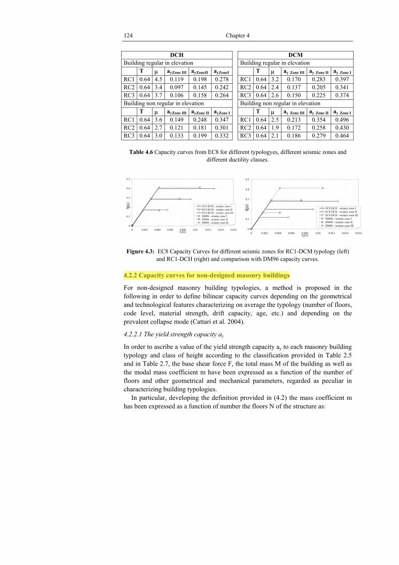
124 Chapter 4
DCH DCM Building regular in elevation Building regular in elevation T µ ayZone III ayZoneII ayZoneI T µ ay Zone III ay Zone II ay Zone I
RC1 0.64 4.5 0.119 0.198 0.278 RC1 0.64 3.2 0.170 0.283 0.397 RC2 0.64 3.4 0.097 0.145 0.242 RC2 0.64 2.4 0.137 0.205 0.341 RC3 0.64 3.7 0.106 0.158 0.264 RC3 0.64 2.6 0.150 0.225 0.374 Building non regular in elevation Building non regular in elevation T µ ayZone III ayZone II ayZone I T µ ay Zone III ay Zone II ay Zone I
RC1 0.64 3.6 0.149 0.248 0.347 RC1 0.64 2.5 0.213 0.354 0.496 RC2 0.64 2.7 0.121 0.181 0.301 RC2 0.64 1.9 0.172 0.258 0.430 RC3 0.64 3.0 0.133 0.199 0.332 RC3 0.64 2.1 0.186 0.279 0.464
Table 4.6 Capacity curves from EC8 for different typologyes, different seismic zones and
different ductility classes.
0
0.1
0.2
0.3
0.4
0.5
0 0.002 0.004 0.006 0.008 0.01 0.012 0.014 0.016Sd[m]
S a[g
]
EC8 DCM - seismic zone IEC8 DCM - seismic zone IIEC8 DCM - seismic zone IIIDM96 - seismic zone IDM96 - seismic zone IIDM96 - seismic zone III
0
0.1
0.2
0.3
0.4
0.5
0 0.002 0.004 0.006 0.008 0.01 0.012 0.014 0.016Sd[m]
S a[g
]
EC8 DCH - seismic zone IEC8 DCH - seismic zone IIEC8 DCH - seismic zone IIIDM96 - seismic zone IDM96 - seismic zone IIDM96 - seismic zone III
Figure 4.3: EC8 Capacity Curves for different seismic zones for RC1-DCM typology (left)
and RC1-DCH (right) and comparison with DM96 capacity curves.
4.2.2 Capacity curves for non-designed masonry buildings
For non-designed masonry building typologies, a method is proposed in the following in order to define bilinear capacity curves depending on the geometrical and technological features characterizing on average the typology (number of floors, code level, material strength, drift capacity, age, etc.) and depending on the prevalent collapse mode (Cattari et al. 2004).
4.2.2.1 The yield strength capacity ay
In order to ascribe a value of the yield strength capacity ay to each masonry building typology and class of height according to the classification provided in Table 2.5 and in Table 2.7, the base shear force F, the total mass M of the building as well as the modal mass coefficient m have been expressed as a function of the number of floors and other geometrical and mechanical parameters, regarded as peculiar in characterizing building typologies.
In particular, developing the definition provided in (4.2) the mass coefficient m has been expressed as a function of number the floors N of the structure as:

A Mechanical based method for European building typologies 125
0.751m 0.75 0.25
N= + (4.20)
The base shear capacity F has been assumed to correspond to the strength offered
by the resistant area aR in the earthquake direction (4.21). It is worth noticing how a 0.5 factor is introduced in the hypothesis that, for a certain earthquake direction, half of the walls are involved:
RF 0.5a= τ (4.21) where τ is the shear strenght [kg/m2] defined as a function of the characteristic shear strenght τ0 and of the compressive strenght σ0 that takes into account the building load and the dead weights τ = τ0(1+ σ0/τ0)0.5.
The resistant area aR is evaluated as a function of the total floor area A introducing a coefficient α:
RaA
α = (4.22)
The coefficient α depends on the building typology but definitely also on the
building floor number being higher for a major number of floors.
Figure 4.4 Resistant areas aR (blue areas, red areas) for two perpendicular directions.
In order to take into account this feature, reference has been made to the ratio
between the upper αΝΑΝ and the ground floor α0Α0 resistant area βN (4.23).
0 0N
N N
AA
αβ =
α (4.23)
It has been possible to express βN as a function of the building floor numbers N,
taking into account geometrical rules belonging to the constructive tradition (rules of

126 Chapter 4
thumbs). N 1 0.2(N 1)β = + − (4.24)
Formula (4.25) provides an example of one of such rules of thumb, where the
wall thickness s is provided as a function of the the building width L and of the building height H over a certain section:
2L Hs c48+
= + (4.25)
where c is a security coefficient.
Considering formula (4.22), (4.23), (4.24) the base shear F can be written as a function of the resistant area of the upper floor and of the number of floors (4.26). A further coefficient ξ is introduced to take into account the non uniform contribution of each masonry panel:
[ ]N N NF 0.5A= ξ α β τ (4.26)
In analogy to what done for the yield strength ay, the building dead weight (plus likely live loads) M, has been expressed in terms of the geometrical and of the mechanical features:
N N
i i i ii i
M A p A h= + α γ∑ ∑ (4.27)
where h is the inter-story height [m], γ is the material density [kg/m3], Ai is the i-
level floor area and pi is the i-level overload. Following the definition of the parameter βN (4.23), a factor βi can be introduced
for each i- level defined as the ratio between the resistant area at i-level αiAi and the resistant area computed at the upper level αNAN.
i ii
N N
AA
αβ =
α (4.28)
In function of βi, and assuming the floor area and the overload constant for each
i-level equation (4.27) can be simplified as:

A Mechanical based method for European building typologies 127
N
ii
M A(Np h )= + γα β∑ (4.29)
Starting from the definition of βN (4.24), it has been possible to express iβ∑ as
a function of the floor numbers N:
1.3i 1 (N 1)β = + −∑ (4.30)
Substituting formula (4.26) and (4.29) in the definition provided for the yield
strength capacity (4.3), ay can be written as:
Ny N
ii
0.5a
m Np h
ταβ ξ=
+ γα β
∑
(4.31)
Moreover, considering, the relations established between the expressions found
for βN (4.24), iβ∑ (4.30) and m (4.20) as a functions of the number of floor N, the
expression found (4.31) can be made explicit in order to clearly recognize the geometrical and the mechanical parameters involved for ay evaluation:
( )
( )
1 1.30 0
y 0.75 1.3
1 Np h 1 (N 1) (0.8 0.2N)a 0.5
(0.75 0.25N ) Np h 1 (N 1)
−
−
τ + τ + γα + − αξ + = ⋅ + + γα + −
(4.32)
4.2.2.2 The true elastic fundamental-mode period of building T
For the evaluation of the elastic period of the structure T reference has been made to EC8 formula (4.15).
For each masonry typology belonging to the assumed classification system (Table 2.5), a characteristic inter-story height h has been defined as well as a CM coefficients (Table 4.7) to be used in place of the the Ct coefficient, recommended by EC8 (Ct=0.05 for masonry building). CM has been defined on the basis of expert judgement, taking into account mechanical characteristics of the materials and the characteristic features of the building i.e. a particular horizontal structure typology or an higher or lower inter-story high.
Alternatively it is possible to make reference to the definition of the fundamental period for a s.d.o.f system (4.33). All the considerations regarding the mechanical and geometrical characteristics features are, in this case, computed into m* and k*,

128 Chapter 4
representing respectively mass and stiffness of the equivalent s.d.o.f system.
m*T 2k *
= π (4.33)
4.2.2.3 The ultimate local displacement du
The structural ductility capacity mainly depends on the material and on the constructive typology. Moreover, the number and the localization of failed masonry panels before the total collapse of the building influence it.
On respects to the building total collapse mode, three limit situations appear as particularly meaningful and are considered:
- lintels failure collapse mode, with almost uniform deformations in masonry piers at the various storeys referred as uniform collapse mode.
- soft-storey collapse mode with prevailing rocking failures - soft-storey collapse mode with prevailing shear failures
With regard to the uniform collapse mode, the ultimate displacement capacity for the s.d.o.f. equivalent structure is given by the equation:
u u yd h d 1NΓ = δ + −
(4.34)
where N is the number of floor, h is the inter-story height Γ is the modal
participation factor for the first natural mode and δu is the ultimate drift ratio In the case of soft-storey collapse mode both for the prevailing rocking failures,
prevailing shear failures, the expression becomes:
u uNhd = δΓ
(4.35)
In particular, developing the definition provided in (4.1) it has been possible to
express the modal participation factor Γ as a function of the number of floors N:
12 1
3 3N
− Γ = +
(4.36)
4.2.2.4 The ultimate strength capacity au
The redistribution of the actions on the uncracked elements can provide an increment of the ultimate strength au as regards to the first yielding value ay (4.37); softening behaviour with a decrement of au can be observed as well.
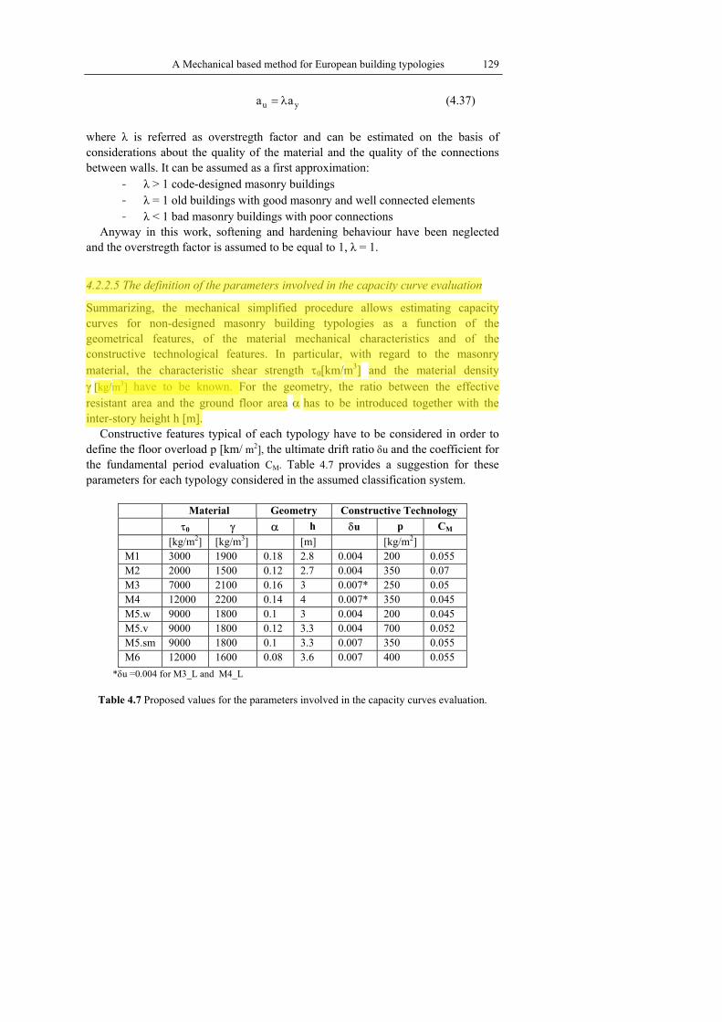
A Mechanical based method for European building typologies 129
u ya a= λ (4.37)
where λ is referred as overstregth factor and can be estimated on the basis of considerations about the quality of the material and the quality of the connections between walls. It can be assumed as a first approximation:
- λ > 1 code-designed masonry buildings - λ = 1 old buildings with good masonry and well connected elements - λ < 1 bad masonry buildings with poor connections
Anyway in this work, softening and hardening behaviour have been neglected and the overstregth factor is assumed to be equal to 1, λ = 1.
4.2.2.5 The definition of the parameters involved in the capacity curve evaluation
Summarizing, the mechanical simplified procedure allows estimating capacity curves for non-designed masonry building typologies as a function of the geometrical features, of the material mechanical characteristics and of the constructive technological features. In particular, with regard to the masonry material, the characteristic shear strength τ0[km/m3] and the material density γ [kg/m3] have to be known. For the geometry, the ratio between the effective resistant area and the ground floor area α has to be introduced together with the inter-story height h [m].
Constructive features typical of each typology have to be considered in order to define the floor overload p [km/ m2], the ultimate drift ratio δu and the coefficient for the fundamental period evaluation CM. Table 4.7 provides a suggestion for these parameters for each typology considered in the assumed classification system.
Material Geometry Constructive Technology τ0 γ α h δu p CM [kg/m2] [kg/m3] [m] [kg/m2] M1 3000 1900 0.18 2.8 0.004 200 0.055 M2 2000 1500 0.12 2.7 0.004 350 0.07 M3 7000 2100 0.16 3 0.007* 250 0.05 M4 12000 2200 0.14 4 0.007* 350 0.045 M5.w 9000 1800 0.1 3 0.004 200 0.045 M5.v 9000 1800 0.12 3.3 0.004 700 0.052 M5.sm 9000 1800 0.1 3.3 0.007 350 0.055 M6 12000 1600 0.08 3.6 0.007 400 0.055
*δu =0.004 for M3_L and M4_L
Table 4.7 Proposed values for the parameters involved in the capacity curves evaluation.

130 Chapter 4
Yield Point Ultimate point Ductility Period dy[m] ay[g] du[m] au[g] µ T
M1 M1-L 0.0017 0.156 0.0119 0.156 6.91 0.211
M1-M 0.0028 0.090 0.0131 0.090 4.67 0.355
M2 M2-L 0.0017 0.096 0.0115 0.096 6.70 0.268
M3-L 0.0028 0.310 0.0131 0.310 4.65 0.192
M3 M3-M 0.0036 0.138 0.0234 0.138 6.58 0.322
M3-H 0.0049 0.103 0.0248 0.103 5.07 0.437
M3-L 0.0026 0.355 0.0170 0.355 6.50 0.173
M4 M4-M 0.0035 0.165 0.0303 0.165 8.78 0.290
M4-H 0.0048 0.124 0.0317 0.124 6.65 0.393
M5.w M5.w-L 0.0030 0.406 0.0132 0.406 4.40 0.173
M5.w-M 0.0050 0.239 0.0153 0.239 3.07 0.290
M5.w-H 0.0069 0.181 0.0173 0.181 2.50 0.393
M5.v M5.v-L 0.0039 0.255 0.0148 0.255 3.75 0.249
M5.v-M 0.0069 0.159 0.0178 0.159 2.57 0.419
M5.v-H 0.0099 0.124 0.0208 0.124 2.10 0.568
M5.sm M5.sm-L 0.0023 0.255 0.0240 0.255 10.34 0.192
M5.sm-M 0.0040 0.154 0.0257 0.154 6.49 0.322
M5.sm-H 0.0056 0.118 0.0274 0.118 4.91 0.437
M6 M6-L 0.0027 0.298 0.0263 0.298 9.67 0.192
M6-M 0.0048 0.184 0.0284 0.184 5.97 0.322
M6-H 0.0068 0.143 0.0304 0.143 4.49 0.437
Table 4.8 Capacity curves defining parameters for unreinforced masonry building typologies for different classes of height.
Different values from the ones provided in table 4.7 can be obviously ascribed to
the building typologies if more in-deapth knowledge is available with regard to the geometry and the material characteristics.
Making reference to the values proposed in table 4.7, capacity curves have been evaluated. Table 4.8 shows the results obtained in terms of yielding and ultimate acceleration and displacement, true fundamental period and ductility capacity.
4.3. PERFORMANCE POINT EVALUATION
The performance of a building to an earthquake depends on the manner its capacity is able to handle the seismic demand.
According to the capacity spectrum method the building performance corresponds to the intersection point, referred as “perfomance point”, between the capacity curve of an equivalent non linear s.d.o.f. system and the demand curve adequately reduced, both represented in a spectral acceleration versus displacement

A Mechanical based method for European building typologies 131
domain (Freeman 1998). The building capacity and the seismic demand are mutually interconnected
depending on the system stiffness and on the system damping variation during the earthquake. Indeed, when a structure overcomes its yield point its effective damping increases, as energy is lost because of the hysteretic damping, as well as its effective period. The structure responds to the ground motion as if it were a more heavily damped, longer-period one. Thus the 5% damped elastic spectrum describing the ground motion has to be reduced to a lower spectrum (representing higher damping) in order to be consistent with the structure response.
This goal can be achieved making reference to overdamped spectra (Freeman 1998, ATC-40 1996) or to inelastic spectra obtained applying reduction factors due to the ductility (Fajfar 1999, Fajfar 2000). The use of overdamped spectra requires the estimation of the equivalent damping as a function of the displacement and the evaluation of the performance point by an interactive procedure. The use of inelastic spectra is easier and have to be, definitly, preferred dealing with a representation of the structure capacity in terms of bilinear capacity curves.
Elastic 5% damped response spectra can be converted into constant-ductility inelastic response spectra applying a strength reduction factor Rµ due to the ductility (Vidic at al. 1994):
aea
SS
Rµ= (4.38)
2
d de a2TS S S
R 4µ
µ= = µ
π (4.39)
Strength reduction factors due to ductility are evaluated in the assumption that the
inelastic spectral displacement Sd remain the same of a perfectly elastic structure Sde (hypothesis referred as ‘the equal displacement approximation).
The intersection of the radial line corresponding to the elastic period of idealized elastic-perfectly plastic system with the elastic 5% damped response spectra Sae defines the acceleration (i.e. the strength) and the corresponding displacement Sde demands required for elastic (linear) behaviour of the system. The yield acceleration Say represents both the acceleration demand and the capacity of the inelastic system. The ratio between the accelerations corresponding to the elastic and inelastic systems represents the strength reduction factor due to the ductility:
ae
ay
S (T)R
Sµ = (4.40)
The ratio between the strength and the displacement of linear and non linear
systems (4.38), leading to the definition of the strength reduction factor Rµ, depends

132 Chapter 4
on the structure stiffness. In particular it is distinguished between flexible and rigid structures respectively characterized by a fundamental period T ≥ TC higher and lower T < TC then the characteristic period of the ground motion TC typically defined as the transition period where the constant acceleration segment of the response spectrum passes to the constant velocity segment.
Te<TC
Te>TCTC
5% damped response spectrum
Sd=Sde Sd Dy
Say
Sae
Sa
µ
Dd
Sad
Spectral Displacement, cm
Spec
tral
Acc
eler
atio
n, g
Figure 4.5 Comparison between capacity curve and inelastic reduced demand curve Formula (4.6) shows how, for flexible structures T ≥ TC the reduction factor Rµ
can be considered approximatively equal to the system ductility µ while for rigid structures T < TC is lower than the ductility (Fajfar 2000).
( ) C
C
C
TR 1 1 T TT
R T T
µ
µ
= µ − + < = µ ≥
(4.41)
In the hypothesis to describe the building capacity in terms of bilinear capacity
curves (where the softening and the hardening behaviours are neglected), and the demand in terms of inelastic response spectra, the performance point, is therefore obtained as:
Cy C
d* y C D2
ae D DD2
T1 (q 1) d T T and q 1
TS qd T T T or q 1
S (T )TT T
4
+ − < > = ≤ < ≤ ≥ π
(4.42)
where TC is the characteristic period of ground motion, TD is the period that
define the constant spectral displacement range, T is the fundamental period of the

A Mechanical based method for European building typologies 133
structure, dy is the yielding displacement of the structure, and q is the ratio between the demand to an elastic system described by the elastic response spectrum Sae (T) and the strength of the non linear structure ay (4.43).
ae
y
Sq
a= (4.43)
4.4 STANDARD SHAPE FOR RESPONSE SPECTRA: THE SEISMIC INPUT REPRESENTATION FOR SYMPLIFIED MECHANICAL METHODS
The use of simplified mechanical approach in the framework of a seismic risk analysis requires an hazard description in terms of an elastic response spectra Sae(T) with a characteristic period TC separating the periods of almost spectral acceleration (T<TC) by the almost constant spectral velocity range (T>TC).
This can be achieved, on one hand, anchoring to hazard analysis, provided in terms of peak ground acceleration ag, predefined spectral shapes related to the local soil conditions, as for instance the one proposed by EC8 (3.21).
On the other hand, the same result can be obtained, fitting response spectra discrete values, provided by predictive equations for fixed periods (Par. 2.2.3), with a standard spectral shape. For the standard shape of the response spectrum, a formulation similar to the one proposed by EC8 is chosen (4.44) in order to be able to determine the displacement at the performance point by the use of (4.42).
g C
Cae g C D
C Dg D2
a 0 T T
TS (T) a T < T T
TT T
a T < T 4sT
≤ ≤
= ≤
≤
(4.44)
The standardized shape in (4.44) consists of four parts: peak ground acceleration
ag, a region of constant spectral acceleration at periods from zero seconds to TC, a region of constant spectral velocity at periods from TC to TD and a region of constant spectral displacement for periods of TD and beyond.
The characteristic period TC, which separates almost constant spectral acceleration (T< TC) by the almost constant spectral velocity range (T> TC), and the period TD which separates the periods of almost constant spectral velocity (T< TD) by the almost constant spectral displacement range (T> TD), have to be determined in such a way to provide the better interpolation to the discrete values resulting from the attenuation laws. TC can be evaluated minimizing the difference between the area of the predictive equation spectrum APE (4.45) and the area under the standard spectral shape ASS (4.46).

134 Chapter 4
( ) ii 1
n 1
PE ae(T ) i 1 iae Ti 1
1A (S S )(T T )2 +
−
+=
= + −∑ (4.45)
In the hypothesis to neglect the region T>TD, and assuming TD=2[s], the area under the standard spectral shape ASS is evaluated according to (4.46).
( ) ( ) ( )max maxSS ae ae(T 0.15) C ae C C aeT 0A 0.075(S S ) T 0.15 S ln(2) ln(T ) T S=== + + − + − (4.46)
Figure (4.6) shows both the spectrum obtained by the AMB96 (2.15) predictive equation for an earthquake magnitude M=7 and a site-source distance r=30 Km and the fitting obtained by the use of the standard spectrum shape (4.44). The characteristic period results in TC=0.4[s].
0
0.1
0.2
0.3
0.4
0.5
0.6
0 0.15 0.3 0.45 0.6 0.75 0.9 1.05 1.2 1.35 1.5 1.65 1.8 1.95 2.1T[s]
Sae[
g]
AMB96 Attenuation Law
Standard Shape
Figure 4.6: Approximation of AMB96 predictive equation spectrum (M=7,r=30km) with the proposed standard shape (TC=0.4[s]).
In the further hypothesis to neglect the region T<TB the standard spectrum shape
has to be evaluated as:
( )SS C a max CA T S 1 ln(2) ln(T )= + − (4.47)
A possible alternative for easily evaluate the periods TC and TD is the one
proposed by HAZUS method (HAZUS 1999) in order to obtain standard shape for attenuation laws response spectra.
According to HAZUS, the region of constant spectral acceleration is defined by spectral acceleration at a period of T=0.3 second Sae(0.3). The constant spectral velocity region is anchored to the spectral acceleration at a period of T=1 second Sae(1). The assumed standard spectral shape can be written as:

A Mechanical based method for European building typologies 135
ae C
ae Cae C D
S (0.3) 0 T TS (T) T
S (0.3) T < T TT
≤ ≤=
≤
(4.48)
Therefore the period, TC can be evaluated by the intersection between the region
of constant spectral acceleration and the region of constant spectral velocity as:
aeC
ae
S (1)T
S (0.3)= (4.49)
The value of TC varies depending on the values of spectral acceleration Sae(0.3)
and Sae(1) that define these two intersecting regions. The constant spectral displacement region is anchored to spectral acceleration at
the period TD, where constant spectral velocity transitions to constant spectral displacement. HAZUS proposes to evaluate TD as a function of the earthquake moment magnitude as shown by the following equation:
M 5
2DT 10
−
= (4.50)
According to this formula TD assumes a value TD=1.77[s] when M=5.5 and a value TD=10[s] when M=7.
Figure 4.7 portrays the approximation of a spectrum obtained from AMB96 attenuation law (M=7, r=30 km) with the standard shape proposed by HAZUS (4.48); the anchorage points Sae(0.3) and Sae(0.1) are indicated. The characteristich period results in TC=0.424 [s].
0
0.1
0.2
0.3
0.4
0.5
0.6
0 0.15 0.3 0.45 0.6 0.75 0.9 1.05 1.2 1.35 1.5 1.65 1.8 1.95 2.1T[s]
Sae[
g]
AMB96 Attenuation Law
Standard Shape
Figure 4.7: Approximation of AMB96 predictive equation spectrum (M=7, r=15km) with HAZUS proposed standard shape (TC=0.424).
The use of a standard response spectrum shape for the representation of

136 Chapter 4
attenuation law spectrum allows simplifying considerably the calculations required to determine building response in terms of the performance point evaluation. It is worth noting that this is a rough approximation and that its application does not allow representing the changes in the shape of the spectrum depending on the earthquake size and on the source-site distance. However, the differences between the shape of an actual spectrum and the proposed standard spectrum tend to be significant only at periods less than 0.3 second and at periods greater than TD. These ranges are usually non meaningful on respect to the fundamental period T characterizing the considered building typologies.
4.5 DAMAGE STATE THRESHOLD DEFINITION
In order to assess which is the damage state suffered by a building typology under a known seismic demand, it has to be established which is the damage state definition that the evaluated performance point overcomes. It is necessary, in other words, to translate numerically the definition of the performance level ascribing to each damage state (Table 2.18).
However, as each one of the capacity curves point represents the structural response to horizontal seismic action (from the initial undamaged elastic behavior through the formation and the development of cracks till the loss of stability), damage states can be defined directly on the capacity curve.
Mean values of the displacement threshold Sd,k (k=1,2,3,4) are proposed for the four damage states (4.51) as a function of the of the yielding dy and of the ultimate du displacements. It is worth noting that the bilinear behaviour is an approximation of the actual curved response, usually made considering an equivalent period (of the cracked structure) and with an equivalent energy dissipation; in particular, the slight damage occurs before yielding, while moderate damage, corresponding to the achievement of the maximum strength, is attained for a spectral displacement greater than dy.
d,1 y
d,2 y
d,3 y u
d,4 u
S 0.7d
S 1.5d
S 0.5(d d )
S d
=
=
= +
=
(4.51)
The definition of the mean value displacement thresholds in (4.51) have been
established on the basis of an expert judgement, and have been then verified on the basis of the results of pushover analyses, performed on prototype buildings from numerical non-linear models.
Comparing the value of the spectral displacement at the performance point Sd* evaluated according to (4.42) with the displacement thresholds definition (4.51) it is

A Mechanical based method for European building typologies 137
possible to establish which is the damage state suffered by a building typology. Figure (4.8) shows, for istance, two different capacity curves, representative of rigid (T<TC) and flexible (T>TC) structures, with the damage state thresholds and the target displacement, obtained by (4.42) in the case of two different demand spectra.
0
0 .1
0 .2
0 .3
0 .4
0 .5
0 0 .01 0.02 0.03 0.0 4 0.0 5 0.0 6S d (m )
S a (g)
a = 0 .1g - T = 0 .5sa = 0 .2g - T = 0 .5sM ona stery (T =0.4 s)
g
C
C
g
ag=0.1 TC=0.5sag=0.2 TC=0.5sCapacity T=0.4
0
0 .1
0 .2
0 .3
0 .4
0 .5
0 0 .01 0.02 0.03 0.0 4 0.0 5 0.0 6S d (m )
S a (g)
a = 0 .1g - T = 0 .5sa = 0 .2g - T = 0 .5sM ona stery (T =0.4 s)
g
C
C
g
ag=0.1 TC=0.5sag=0.2 TC=0.5sCapacity T=0.4
0
0.1
0.2
0.3
0.4
0.5
0 0.01 0.02 0.03 0.04 0.05 0.06Sd (m)
S a (g
)
a =0.1g - T =0.5sa =0.2g - T =0.5sTower (T=0.7s)
g
CC
g
ag=0.1 TC=0.5sag=0.2 TC=0.5sCapacity T=0.7s
0
0.1
0.2
0.3
0.4
0.5
0 0.01 0.02 0.03 0.04 0.05 0.06Sd (m)
S a (g
)
a =0.1g - T =0.5sa =0.2g - T =0.5sTower (T=0.7s)
g
CC
g
ag=0.1 TC=0.5sag=0.2 TC=0.5sCapacity T=0.7s
Figure 4.8 Capacity curves, damage state thresholds and evaluation of the target displacement
for rigid (T<TC) and flexible structures (T>TC), for two demand spectra.
4.6 UNCERTAINTIES AFFECTING THE SYMPLIFIED MECHANICAL METHOD DAMAGE EVALUATION
The performance point Sd* (target displacement) obtained by (4.42) represents a median estimate of the structure spectral response. The variability of the subsequent estimation of the damage suffered by the building, resulting from the comparison with the damage state thresholds (4.51), depends on the uncertainties associated in drawing capacity curve, in defining damage states and finally in predicting the ground shaking.
According to HAZUS (1999) approach, the uncertainties in damage prediction can be represented by lognormal fragility curves, as a functions of the expected performance displacement Sd* and of the mean displacement limit states Sd,k:
d*Sk d*
k d,k
S1D S lnS
P =Φ β
(4.52)
where Φ is the normal cumulative distribution function and βk is the normalized
standard deviation of the natural logarithm of the displacement threshold Sd,k. According to Kircher et al. (1997), the total variability associated to each
structural damage state βk, depends jointly by three contribution: the lognormal standard deviation parameter that describes the variability of the capacity curve βC, the lognormal standard deviation parameter that describes the variability of the demand spectrum βD and the lognormal standard deviation parameter βSd,k that describes the uncertainty in the estimate of the threshold for the structural damage

138 Chapter 4
state Sd,k. The combination of these three parameters has been obtained by a complex process of convolving probability distributions of the demand spectrum and of the capacity curve.
( ) ( )d,k
22k C D SCONV ,β = β β + β (4.53)
Assuming that the capacity and the demand are independent variables, a
simplified form for the evaluation of the total variability may be obatined considering the square root sum of the square value (SRSS) of all the three uncertainty contributors:
dk
2 2 2k C D Sβ = β + β + β (4.54)
Anyway, because of the difficulty in determining the uncertainty in the estimate
of βSd,k (assumed by HAZUS βSd,k≈0.4), an alternative approach is proposed. The idea is to evaluate the overall uncertainty in the damage estimation βk in such
a way that it can represents the same dispersion of observed damage data, that, as already said, are well fitted by a binomial distribution (3.1). Reference is made to the four mean damage values µk (Table 5.1) providing binomial distributions with a 50% occurrence probability for each damage state P[Dkµk]=0.5 with k=1÷4. For each of the obtained distribution the occurrence probability for the other damage states is evaluated (i.e. for the distribution providing P[D1µ1]=0.5 are then evaluated the occurrence probabilities for D2, D3 D4: P[D2µ1], P[D3µ1], P[D4µ1]).
The resulting probabilities are assumed for representing the damage probabilities derived from the mechanical approach (4.52) P[Dkµk]=P[DSkSd*] (i.e. P[D1µ1]=P[DS1Sd*],P[D2µ1]=P[DS2Sd*],P[D3µ1]=P[DS3Sd*],P[D4µ1]=P[DS4Sd
*] where Sd*= Sd,1). Thus βk is evaluated forcing the lognormal fragility curves defined as (4.52) to
pass closely to the probabilities obtained from binomial distributions (points in figure 4.9).

A Mechanical based method for European building typologies 139
Sd,4Sd,3Sd,2Sd,10
0.1
0.2
0.3
0.4
0.5
0.6
0.7
0.8
0.9
1
Sd [m]
P(D
>Dk)
Figure 4.9 Points in this figure correspond to the damage state probabilities obtained by
binomial distributions and lines are the fitting lognormal fragility curves.
Repeating this procedure for different buildings typologies it has been observed that βk depends on the ductility µ characterizing the capacity curve (4.55).
k 0.4 lnβ = µ (4.55)
In the framework of the macroseismic approach it has been considered the possibility to differently defining the scatter of the final damage distributions depending on the amount of the cognitive uncertainties characterizing the vulnerability assessment. According to the procedure here described for the evaluation of the βk the same results can be achieved, forcing lognormal fragility curves to fit distribution differently scattered on respect to the binomial distribution that have lead to the definition of equation (4.55).
For instance, the correlation between βk and the building typology ductility µ in (4.56) has been obtained forcing lognormal fragility curves on a beta fragility (3.4) curves characterized by a parameter t=4.
k 0.62 lnβ = µ (4.56)
The values obtained applying these formulas are consistent with the ones βk=0.65 ÷1.2 proposed by HAZUS (that, anyway, do not strictly depend on the building ductility). As a matter of fact, for a building ductility capacity in the range of µ=2.5÷8 the βk values provided by the proposed formulas range over βk=0.37÷0.83 for (4.55) and over βk=0.57÷1.29 for (4.56).

140 Chapter 4
4.7 SIMPLIFIED MECHANICAL METHOD: DAMAGE AND LOSS DISTRIBUTIONS AND FRAGILITY CURVES
Once the target displacement Sd* (4.42), the displacement thresholds Sd,k (4.51), and the normalized standard deviation βk (4.55) have been evaluated, the evaluation of damage fragility curves according to the proposed simplified mechanical method is a straightforward operation (4.57).
In particular, if the hazard scenario is defined only by the peak ground acceleration ag, fixing the spectral shapes for one or a limited number of soil conditions, the fragility curves may be expressed directly as a function of ag:
gSk g
k g,k
a1D a lna
P =Φ β
(4.57)
where ag,k is the ground acceleration that produces the damage state Sd,k
(k=1,2,3,4) The probability histograms of the estimated median damage states are given by:
*
* *
*
S4 S4 d
Sk Sk Sk+1d d
S0 1 d
p D S
p D S D S k=1 3
p 1 D S
P
P P
P
= = − ÷
= −
(4.58)
Comparing the definitions provided for damage state (DSk) and macroseismic
method damage grades (Dk) (Table 2.19), a direct correspondence of the first three levels can be observed, while the last two damage grades can hardly be distinguished in a mechanical model and for this reason are grouped together in the complete damage state DS4.
Thus, the probability histograms of the damage limit states pSk can be considered substantially equivalent to the probability histograms of the damage grades pk for the first three damage levels:
k Skp p k 1 3 = = ÷ (4.59)
On the other hand, in order to take out from the probability pS4 the part that
corresponds to the building collapse p5 the procedure described in the following is proposed. The idea is to evaluate the part that corresponds to the building collapse p5 in such a way to obtain p4 and p5 in the same proportions characterizing a binomial function.
A parameter η is therefore defined in order to measure the share between the probability to have building collapse p5 on respect to the sum of p4 and p5 probability

A Mechanical based method for European building typologies 141
according to the binomial distribution:
5
4 5
pp p
η =+
(4.60)
It has been found that this ratio can be expressed as a function of the binomial
mean damage grade µ D evaluated on respect to the first four grades Dk (k=1÷4). ( )D0.09senh 0.6η = µ (4.61)
Assuming the same share for ps4 probability to have a damage state DS4, the following correspondences can be established:
( )5 DS S4
4 S4 5
p 0.09senh 0.6 p
p p p
= µ
= − (4.62)
where µ DS is the mean value of the probability histograms of damage states DSk
(k=1÷4).
4
DS kk 1
kP=
µ = ∑ (4.63)
Fragility curves and the corresponding histograms of damage state probability are
shown in Figure 4.10 for the two different values of the peak ground acceleration; in light grey it is represented the share of pS4 that is assumed as destruction (D5), according to (4.60).
0
0.2
0.4
0.6
0.8
1
0 0.02 0.04 0.06 0.08Sd (m)
P[D
k|Sd*
]
D1D2D3D4
0
0.1
0.2
0.3
0.4
0.5
0 1 2 3 4 5Dk
P k
a =0.1ga =0.2g
g
g
Figure 4.10 Fragility curves and damage distribution before and after the damage repartitions for the capacity and the demand curves in Figure 4.8. Fragility curves are the ones drawn for
building typology characterized by T=0.7[s].

142 Chapter 4

Macroseismic and Mechanical methods: comparable approaches 143
CHAPTER 5
MACROSEISMIC AND MECHANICAL METHODS: COMPARABLE
APPROACHES
5.1. THE SEIMIC INPUT GENERATING DAMAGE STATES ACCORDING TO MACROSEISMIC AND MECHANICAL METHODS
The Macroseismic and the Mechanical models are different for derivation and conception and as well differ in the way they are implemented. Nevertheless in this chapter they are examined aiming to their comparison and to their reciprocal calibration. The comparison is performed in order to verify that the two methods provide results equivalent and coherent. The reciprocal calibration allows taking into account in each one of the two methods the positive features characterizing the other. Considering the Mechanical model, thus means for instance to have the chance to verify and to calibrate capacity curves on respect to the observed data. On the other hand, the Macroseismic Method could be improved in such aspects that are well represented by the Mechanical approach like the possibility to differently characterise the ductility of buildings drawn according to different seismic codes or the different dynamic behaviours observed for the same building typology characterized by a different height or a different type of horizontal structures.
The comparison begins considering the Mechanical method and the Macroseismic method common aspects. First of all, both the methods refer, in their application, to the same building typology classification (Table 2.5). Beyond that, they describe damage in a similar way, as the four mechanical damage limit states, related to performance level of the structure, can be as well associated to the macroscopic evidence of the damage, to which Macroseismic method refers to (Table 2.19).
It is worth underling that none of the two methods has been considered more reliable and assumed as the reference approach; the comparison has been performed looking for an equivalence of the results in term of the damage evaluated implementing the Macroseismic and the Mechanical approach.
Thus, for both the methods, values of the seismic input causing the same damage grade with 50% occurrence probability P[Dk] = 0.5 are evaluated.
For the Macroseismic method it means to look for the macroseismic intensity Ik, as a function of the vulnerability index V and of the ductility index Q, causing a mean damage grade µ k corresponding to a 50% occurrence probability for a k-damage grade Dk.

144 Chapter 5
( ) [ ]k k kI f V Q D 0 5, P .= → µ → = (5.1)
For the Mechanical method it means to look for the peak ground acceleration ag,k function of the parameters defining soil conditions (s, TC) and of the parameters describing capacity curves (ay, T, µ), that are able to cause a building displacement equal to a certain k-damage limit state threshold Sd*= Sd,k.
( )g k C y d d ka f s T a T S S, * ,, , , ,= µ → = (5.2)
5.1.1 Evaluation of the intensities Ik according to the Macroseismic method
According to the Macroseismic method, the building behaviour is described by two parameters: the vulnerability index V, that provides a measure of the building weakness to the seismic actions, and the ductility index Q, which controls the rate of the damage increase with the intensity. The seismic action is described in terms of a macroseimic intensity I and the damage description is summarized by a mean damage grade µD.
Once the building vulnerability is assessed, so that the vulnerability index V and the ductility index Q are known, the expected damage grade µD, is evaluated for a given intensity I (3.11). The probabilities pk of having each of the considered damage grades Dk k=1÷4 are distributed around this mean value µD according to a beta distribution (3.4). For the sake of an easier implementation, reference has been made to the binomial function (3.1) rather then to the beta function (3.4); as a matter of fact, the binomial function has been also employed developing vulnerability curves (Par. 3.1.4) and it is almost equivalent to the beta distribution when a parameter t = 7 is introduced.
Table 5.1 shows mean damage values µDk causing a 50% occurrence probability P[Dk]=0.5 for the different damage grades Dk k=1÷4 according to the binomial distribution.
D1 D2 D3 D4
µD1 = 0.65 µD2 = 1.55 µD3 = 2.5 µD4 = 3.44
Table 5.1 Mean damage values µDk causing P[Dk]=0.5 according to the binomial distribution.
Mean values µDk and damage grades Dk are linearly correlated:
Dk k0 93D 0 28µ = −. . (5.3)
Intensities Ik causing damage grade Dk with a 50% occurrence probability P[Dk]=0.50 are evaluated substituting equation (5.3) into the formula describing vulnerability curves (3.11) according to the Macroseismic method:

Macroseismic and Mechanical methods: comparable approaches 145
( )k kI 13 1 6 25V Q 0 372D 1 112= − − −. . arctanh . . (5.4)
In particular for the damage grades D1, D2, D3, D4, formula (5.4) can be written
as:
1I 13 1 6 25V 0 95048Q= − −. . . (5.5)
2I 13 1 6 25V 0 38611Q= − −. . . (5.6)
3I 13 1 6 25V 0 004Q= − +. . . (5.7)
4I 13 1 6 25V 0 39539Q= − +. . . (5.8)
Table 5.2 shows macroseimic intensity values I1 and I4 causing respectively damage D1 and damage D4 for masonry building typologies according to the Macroseimic approach.
Q V I1 I4 M1 2.3 0.87 5.5 8.6 M2 2.3 0.84 5.7 8.8 M3 2.3 0.74 6.3 9.4 M4 2.3 0.62 7.1 10.2 M5 2.3 0.74 6.3 9.4 M6 2.3 0.62 7.1 10.2 M7 2.3 0.45 8.1 11.2
Table 5.2 I1 and I4 intensity values for masonry building typologies.
5.1.2 Evaluation of the acceleration values ag,k according to the Mechanical method
In the hypothesis to neglect the building softening and hardening behaviour, typological capacity curves are defined by three parameters: the fundamental period T, the yielding spectral acceleration ay and the ductility capacity µ.
Assuming a predefined spectral shape related to the local soil conditions, the hazard scenario is completely described by the peak ground acceleration ag, by the characteristic period TC, which separates the periods of almost constant spectral acceleration T<TC by the almost constant spectral velocity range T>TC and by a soil factor s (where sag is the top value of the acceleration spectrum).
The displacement limit states defined in (4.51) represent, from a probabilistic point of view, mean values of the damage states thresholds with a 50% occurrence

146 Chapter 5
probability P[Sdk]=0.50. Thus, once the spectral shape is defined, the peak ground accelerations ag,k causing k-damage limit state with a 50% occurrence probability are the ones for which the displacement at the performance point Sd* is equal to the k-limit states threshold Sd* = Sd,k. This means that the peak ground accelerations ag,k (k =1÷4) are obtained from the identity between the equations defining damage limit state thresholds Sd,k (4.51) and formula for the evaluation of the displacement at the performance point Sd* (4.42). It goes without saying that, as the performance point displacement is differently determined for rigid T<TC and for flexible structures T≥TC, the peak ground accelerations ag,k have to be evaluated in a different way for these two cases.
Formula (5.9÷5.12) provide the peak ground accelerations agk inducing the four damage states for rigid structures T<TC in the case q>1 (4.43).
g 1 y CC
0 7a a TsT,
.= (5.9)
yCg 2
C
a TTa 0 5
T sT, . = +
(5.10)
yCg 3
C
a T2Ta 0 5 1
T sT, . = µ − +
(5.11)
yCg 4
C
a TTa 1
T sT, = µ − +
(5.12)
Formula (5.13÷5.16) provides the peak ground accelerations ag inducing the four
damage states for flexible structures T≥TC and q ≤1 (4.43).
yg 1
c
a Ta 0 7
sT, .= (5.13)
yg 2
c
a Ta 1 5
sT, .= (5.14)
( ) yg 3
c
a Ta 0 5 1
sT, .= + µ (5.15)
yg 4
c
a Ta
ST, = µ (5.16)

Macroseismic and Mechanical methods: comparable approaches 147
5.2 EQUIVALENCE BETWEEN THE TWO METHODS
According to the Macroseismic method the seismic input is described in term of the macroseismic intensity. On the other hand, the Mechanical method refers to inelastic response spectra. Therefore, aiming to compare the two approaches, it can not be left aside to look for a correlation between these two seismic input parameters. As a matter of fact, assuming a predefined spectral shape related to soil conditions, response spectra are completely determined once the peak ground acceleration ag is known. Thus it is sufficient to establish a correlation between the intensity I and the peak ground acceleration ag.
Once a I-ag correlations has been assumed, parameters defining capacity curves can be derived from the ones defining vulnerability curves and vice-versa imposing the equivalence between the seismic inputs causing the same damage conditions.
In particular, reference has been made to (I1, ag1) and to (I4, ag4) derived respectively for damage D1 and for damage D4 as the definition and the identification on the capacity curve of these two damage levels are considered more reliable.
Deriving the Mechanical method from the Macroseismic method, it must be taken into consideration that one of the parameters defining the Mechanical approach must be assumed as known, as the parameters defining the vulnerability curve are two (V, Q) instead of the three parameters (T, ay, µ) defining the capacity curves.
5.2.1 A common formulation for Intensity-PGA correlations
It has been stated that, in order to establish an equivalence of the results obtained implementing the Macroseismic and the Mechanical approach, it is necessary, first of all, to set a correlation between the intensity I and the peak ground acceleration ag. These parameters are completely different, being the second a physical parameter of the motion, variable from point to point due to the local soil conditions, and the former a subjective measure, average in a wide area, that implicitly includes the vulnerability itself (even though EMS-98 macroseimic scale tries to overcome this limitation). Making reference to some correlations (summarized in Par. 2.2.1.4) between the wide ranges of the ones proposed in literature it clearly appears how they are extremely scattered (Figure 2.2). Anyway it has been observed that most of the analytical relations may be expressed in a similar form, in particular the peak ground acceleration ag can be related to the Macroseismic Intensity I according to the following function: ( )I 5
g 1 2a c c −= (5.17)
Consequently the macroseismic intensity I can be related to the peak ground acceleration ag by a logarithmic function:

148 Chapter 5
( )g 12
1I 5 lna lnclnc
= + - (5.18)
where c2 represents the base of the power function (5.17) and the base of the
logarithmic function (5.18) while c1 is a multiplier factor. In particular, having assumed that the correlations are defined starting from an intensity I=V, c1 represents the peak ground acceleration value ag corresponding to this reference intensity. On the other hand, c2 measures the rate of the peak ground acceleration increase with the intensity; in particular, considering a one degree variation for the macroseismic intensity ∆I =1, the corresponding acceleration multiplier factor fag is equal to fag=c2. Table 5.3 shows the values assumed by the parameters c1 and c2 for different I-ag correlations (Par. 2.2.1.4).
I-ag correlation 1c 2c
Guarenti-Petrini (2.2) 0.018 1.8 Margottini (2.3) 0.04 1.5 Murphy (2.5) 0.03 1.5 Assumed correlation 0.03 1.6
Table 5.3 Values of c1 and c2 parameters for different I-ag laws.
In the same table, a I-ag law intermediate between Guagenti and Petrini (2.2) and
Margottini (2.3) correlations is proposed [c1=0.03 and c2=1.6].
0.0
0.1
0.2
0.3
0.4
0.5
5 6 7 8 9 10 11EMS-98 Intensity
PGA
[g]
Assumed Correlation
Margottini
Murphy-O'Brien
Guagenti-Petrini
Figure 5.1 Different I-ag correlations and their representation in terms of the proposed formulation (5.17).

Macroseismic and Mechanical methods: comparable approaches 149
Lower values for the parameter c2 correspond to flattened curves. A flattened curve means that for a same damage increment, induced by a variation of the macroseismic intensity, the corresponding variation in term of the peak ground acceleration is lower. In other words it means that, on respect to steeper I-ag correlations, it is sufficient a lower peak ground acceleration multiplier factor fag to produce an increase in the observed damage.
On respect to the formulation provided for I-ag laws (5.17), the following relations exist between the multiplier factor fag of the peak ground acceleration ag and the macroseismic intensity increments ∆I. To each multiplier factor fag a macroseimic intensity increment ∆I corresponds (5.19) and vice-versa (5.20).
( )
( )( )
11 0
g 0
I 5g1 I I I2
a 2 2I 5g0 2
a cf c c
a c
−− ∆
−= = = = (5.19)
a
2
lnfI
lnc∆ = (5.20)
5.2.2 Deriving the Macroseismic method vulnerability curves from the Mechanical method capacity curves
Equivalent vulnerability curves can be evaluated once capacity curves, describing building capacity according to the mechanical method, are defined. The peak ground accelerations ag1 and ag4 able to generate, respectively, slight damage D1 and collapse D4 with a 50% occurrence probability for an assumed capacity curve, are evaluated as a function of the fundamental period T of the yielding spectral acceleration ay and of the ductility capacity µ, according to equations (5.9) and (5.12) for rigid structure T<TC and equations (5.13) and (5.16) for flexible structure T≥TC.
To the ag1 and ag4 peak ground accelerations, macroseismic intensities I1 and I4, able to generate damages D1 and D4 with a 50% occurrence probability correspond, according to the assumed formulation for the I-ag law (5.17)
( )1 g 1 12
1I 5 lna lnclnc ,= + − (5.21)
( )4 g 4 12
1I 5 lna lnclnc ,= + − (5.22)
Intensities I1 and I4 in formulas (5.21) and (5.22) can be expressed as a function
of the macroseismic method parameters V and Q according to formulas (5.5) and (5.8) respectively. Substituting in (5.21), equation (5.5) and equation (5.9) for rigid

150 Chapter 5
structure (T<TC) or equation (5.13) for flexible structure T≥TC and substituting in (5.22) equation (5.8) and equation (5.12) for rigid structure T<TC or equation (5.16) for flexible structure T≥TC, the Macroseismic method parameters V and Q are obtained as a function of the Mechanical method parameters T, ay, µ and of the parameters describing soil conditions (the characteristic period of the ground motion TC and the soil factor s):
2
2
2
2
yC
1C
CC
C
yC
1 CC
C
a1V 8.1 0.95Q ln6.25 1.43sc
T TT1 TQ ln 1
1.35 T 0.7T
a1 TV 8.1 0.95Q ln6.25 1.43sc T
T T1Q ln
1.35 0.7
= − −
< = = µ − +
= − −
≥ = µ =
(5.23)
It can be noticed how, coherently with its meaning, the ductility index Q is only
function of the ductility capacity µ and of the parameter c2 measuring the amount of the peak ground acceleration factor fag causing damage progression.
It is worth noticing that according to (5.23) the behaviour modifier factor ∆V, introduced in the framework of the Macroseismic approach (Par 3.3.2) to account for the different building features influencing its seismic behaviour, can be derived or verified as a function of the variation of the Mechanical model parameters. An increment or a decrement in the building yielding acceleration ay, on respect to the average value characterizing the building typology ay0, caused by the presence of a particular feature increasing the strength of the building or its weakness can be, indeed, translated in terms of a behaviour modifier factor:
ya
2
ln(f ) 1V
ln(c ) 6.25∆ = (5.24)
where y0
ya
y
af
a= for rigid structure (T<TC) and y
0 0
ya
y
a Tf
a T= for flexible
structure (T≥TC).
Thus, an increment in the yielding acceleration ay causes a yielding acceleration factor
yaf 1> to which a decrease in the building vulnerability corresponds ∆V<0.

Macroseismic and Mechanical methods: comparable approaches 151
fay ∆V c2=1.5 c2=1.6 c2=1.7 c2=1.8- 0.01 1.026 1.030 1.034 1.037 -0.02 1.052 1.061 1.069 1.076 -0.04 1.107 1.125 1.142 1.158 -0.06 1.164 1.193 1.220 1.247 -0.08 1.225 1.265 1.304 1.342 -0.16 1.5 1.6 1.7 1.8
Table 5.4 Yielding acceleration factors fay corresponding to behavior modifier factors ∆V for
different values of the parameter c2.
5.2.3 Deriving the Mechanical method capacity curves from the Macroseismic method vulnerability curves
Equivalent capacity curves can be evaluated once vulnerability curves, describing building vulnerability according to the Macroseismic method, are defined. As the Macroseismic method is defined by two parameters (V and Q) one of the three parameters (T, Ay, µ) defining the Mechanical method have to be assumed. The easiest parameter to be estimated by expert judgement is the fundamental period T that is moreover the one with the lowest influence on the displacement demand evaluation.
The macroseismic intensities I1 and I4 able to generate the slight damage D1 and the collapse D4 for the assumed vulnerability curve are evaluated according to (5.5) and (5.8). Making reference to the common formulation proposed for I-ag correlations (5.17) the ag1 and ag4 peak ground accelerations corresponding to I1 and I4 macroseismic intensities are evaluated as:
( )1I 5
g 1 1 2a c c −=, (5.25)
( )4I 5g 4 1 2a c c −=, (5.26)
Accelerations ag1 e ag4 are correlated to the parameters defining the capacity curve
ay, T and µ according to the equations (5.9) and (5.12) for rigid structures (T<TC) and to (5.13) and (5.16) for flexible structure T ≥ TC.
By imposing that the two approaches give the same results for the damage levels D1 and D4 and assuming that the fundamental period T is known, the parameters defining a capacity curve equivalent to the assumed vulnerability curve are so derived:

152 Chapter 5
(8.1 6.25V 0.95Q)y 1 2
C 1.35QC C2
(8.1 6.25V 0.95Q) Cy 1 2
C1.35Q2
a 1.43 c cT T T T1 0.7 cT T
Ta 1.43 c c TT T0.7c
s
s
− −
− −
=< µ = − + =≥ µ =
(5.27)
It is worth noting that, the yielding spectral acceleration ay mainly depends on the
vulnerability index V, while the ductility capacity µ is correlated only to the ductility index Q that influence the rate of damage increase with the intensity.
5.2.4 Damage limit states and damage grades equivalence
According to the Mechanical method, the definition of the damage limit state thresholds for slight Sd1 and complete damage Sd4 is quite obvious as slight damage state Sd1 is identified before the achievement of the yielding point dy and the complete damage state Sd4 corresponds to the achievement of the ultimate displacement du.
The identification on the capacity curve of the intermediate extensive Sd2 and moderate Sd3 damage limit states is less obvious. Their definition has been derived in the following imposing the same damage progression characterizing the Macroseismic method.
It has been assumed that the moderate Sd2 and the extensive Sd3 damage limit states are defined depending on the yielding displacement dy as a function, respectively, of the coefficient θ2 and θ3:
d,2 2 yS d= θ
d,3 3 yS d= θ (5.28)
The acceleration ag2, able to generate the moderate damage limit state Sd2, is obtained as a function of the parameter θ2 equalling (5.28) to the equation for the performance point evaluation (4.42):
yg,2 2
c
a Ta
sT= θ (5.29)
Equation (5.29) can be written, as well, as a function of the macroseismic
intensity I2 by the use of the proposed formulation for the I-ag laws (5.17):

Macroseismic and Mechanical methods: comparable approaches 153
2 y(I 5)1 2 2
c
a Tc c
sT− = θ (5.30)
The quantity ayT in equation (5.30) can be expressed as a function of the
Macroseismic intensity I1 evaluating the equality expressed in equation (5.30) on respect to slight damage limit state Sd1:
1(I 5)cy 1 2
sTa T c c
0.7−= (5.31)
Substituting (5.31) in (5.30) it results:
( )2 1I I2 20 7c. −θ = (5.32)
From equations (5.5) and (5.6), providing respectively macroseismic intensities I1
and I2 as a function of the Macroseismic parameters V and Q, equation (5.32) can be expressed as:
0 564 Q
2 20 7c .. ⋅θ = (5.33)
Thus, considering the correlation existing between the building ductility µ defined in the framework of the mechanical approach, and the Macroseismic ductility index Q in the case of flexible structures T≥ TC (5.23), equation (5.30) can be written as a function of the ductility capacity µ.
0 41933
2 0 813 ..θ = µ (5.34)
The same procedure can be followed considering rigid structures T<TC. In this case θ2 depends not only on the parameters describing the capacity curves (the fundamental period T and the ductility capacity µ) but also on the characteristic period of the ground motion TC.
0 58067 0 41933
c c c2
T T T1 0 813 1
T T T
. .
. θ = − + µ − +
(5.35)
The procedure to be applied for determining θ3 is identical to the one, previously
described, followed for the evaluation of θ2. Equations for θ3 are respectively (5.63) for rigid structure and (5.37) for flexible structure:

154 Chapter 5
0 7093 C0 9 T T.. θ = µ ≥ (5.36)
0 291 0 709
c c c3 C
T T T1 0 9 1 T T
T T T
. .
. θ = − + µ − + <
(5.37)
For the sake of an easier and clearer implementation of the Mechanical method, it
is preferable to have damage limit state thresholds defined independently from the parameters describing soil condition. For this reason it has been assumed to make reference to the definition of θ2 and θ3 derived in the case of flexible structures (T<TC).
0 42
d 2 2 y yS d 0 8 d= θ = µ ., . (5.38)
0 709
d 3 3 y yS d 0 9 d= θ = µ ., . (5.39)
Therefore, according to the comparison between the Macroseismic and the
Mechanical approach, it can be asserted that, in order to have in the Mechanical method the same damage progression characterizing the Macroseismic method, the damage limit state thresholds have to be defined as in formulas (5.38) and (5.39). Comparing equations (5.38) and (5.39) with the damage limit state definitions provided in Chapter 4 (4.51), it comes out, on average, a good agreement; this confirms the reliability of the Sd,k definitions adopted in the framework of the Mechanical model.
5.3 A PROPOSAL FOR EQUIVALENT MACROSEISMIC AND MECHANICAL METHODS
The Macroseismic and the Mechanical methods have been derived in a conceptually rigorous way and independently one from the other (Chapter 3 and chapter 4 respectively). Nevertheless, Macroseismic method defining parameters can be related to the Mechanical ones (5.23) and vice-versa (5.27) looking for the seismic input providing for the two methods equivalent result in terms of the damage estimation ad assuming an I-ag correlation. Therefore the Macroseismic and the Mechanical methods defining parameters compared and tuned according to formulas (5.23) and (5.27) lead to the definition of “equivalent Macroseismic and Mechanical methods” in the sense that they are expected to provide equivalent results in terms of damage scenarios when implemented on respect to coherent hazard descriptions.
In order to define these equivalent Macroseismic and Mechanical methods the macroseismic method parameters (V and Q) have been, thanks to the comparison with the Mechanical method, refined and further detailed, with regards the sub-typologies not accounted for by the EMS-98 classification system. The Mechanical method equivalent to this new-defined Macroseismic method has therefore been

Macroseismic and Mechanical methods: comparable approaches 155
derived according to formula (5.27). It is worth noting how the equivalence between the two approaches cannot be established in an unambiguous way depending on the choice of the I-ag correlation that is function of the two parameters c1 and c2.
In any case, the assumed I-ag correlation [c1=0.03 and c2=1.6] shown in Figure 5.1 can be considered the most suitable one to be employed. The fact that the two methods, both reliable, have proved to be equivalent if compared with respect to this I-ag correlation has been considered, indeed, an implicit validation for the correlation itself. Equivalent mechanical method defining parameters have been moreover derived for Guagenti and Petrini (1989) I-ag law [c1=0.018 and c2=1.8].
It is worth noting that the equivalent methods, hereby derived in the hypothesis of a rigid soil, can be easily defined for other soil conditions. The amplification effects are indeed represented equivalently by the two approaches; the macroseismic method soil modifiers are, indeed, derived from the response spectra related to soil conditions employed in the framework of the mechanical approach.
5.3.1 Equivalent Macroseismic and Mechanical methods for masonry building typologies
5.3.1.1 Masonry building capacity curves derived from the Macroseismic method
Proposing the simplified mechanical model for masonry building capacity curves (Par. 4.2.2), some assumptions have been made about the prevalent collapse mode, the material mechanical characteristics and the geometrical features. In order to verify these hypotheses and the reliability of the procedure followed, mechanical capacity curves have been compared with the capacity curves derived according to (5.27) from the Macroseismic method (referred in the following as macroseismic capacity curve) making reference to the vulnerability V and to the ductility Q indexes in table (3.4). The macroseismic capacity curves have been drawn for rock soil conditions (Tc=0.4 s=2.5) and assuming for the building typologies, the same fundamental period T resulting in the mechanical approach (Table 4.8). The macroseimic capacity curves have been proved to be coherent and compatible with the ones defined in the framework of the mechanical models. Figure 5.2 shows macroseismic capacity curves obtained for M1 and M5 typologies employing two different I-ag correlations [c1=0.018; c2=1.8] and [c1=0.03, c2=1.6] according to (5.17).

156 Chapter 5
0
0.05
0.1
0.15
0.2
0.25
0 0.005 0.01 0.015 0.02 0.025Sd[m]
Sa[g
]
M1-MMacro M1-M [c1=0.018 c2=1.8]Macro M1-M [c1=0.03 c2=1.6]
0
0.05
0.1
0.15
0.2
0.25
0 0.005 0.01 0.015 0.02 0.025Sd[m]
Sa[g
]
M5.w_MMacro M5 [c1=0.018 c2=1.8]Macro M5 [c1=0.03 c2=1.6]
Figure 5.2 Comparison between macroseismic and mechanical capacity curves for M1 and
M5 building typology. It is worth noting how macroseismic capacity curves, deduced making reference
to [c1=0.03, c2=1.6] I-ag law, are characterized by a higher resistance (yielding acceleration ay) and a lower ductility capacity µ. Thus can be easily explained remembering the meaning of the parameters c1 and c2 of the I-ag correlation (5.17).
In particular c2 represents the value of the acceleration factor fag corresponding to a macroseismic intensity increment ∆I=1. Deriving capacity curves from the Macroseimic approach, the ductility capacity µ is influenced only by the parameter c2 (thus a lower ductility capacity results employing a I-ag correlation with c2=1.6 rather then a I-ag correlation with c2=1.8). In other words, a flattened I-ag correlation (a lower value of c2) means that a lower value of fag is sufficient to generate the same damage progression, measured in terms of a ∆I=1, on respect to a deeper correlation (Fig. 5.1). According to this reasoning, flattened I-ag correlations should have been defined in geographycal areas where the building stock is characterized by a lower ductility capacity.
The yielding acceleration ay is influenced both by the parameters c1 and c2; indeed, the higher value of c1 for the [c1=0.03, c2=1.6] I-ag correlation on respect to the [c1=0.02, c2=1.8] I-ag correlation causes the higher values in the evaluated yielding accelerations ay.
5.3.1.2 Masonry building vulnerability curves derived from the Mechanical method
The capacity curves defined in the framework of the mechanical approach can be represented in terms of vulnerability curves translating the defining parameters (T, ay, µ) in terms of the vulnerability V and the ductility Q indexes, according to (5.23).
Table 5.5 shows the results obtained for rock soil condition (Tc=0.4 s=2.5) employing [c1=0.018; c2=1.8] and [c1=0.03, c2=1.6] I-ag correlations. The similarity between the vulnerability index average values of V obtained in this way and the vulnerability index V values evaluated in the framework of the Macroseismic method (italics characters) can be regarded as a reciprocal validation of the two proposed vulnerability approaches.

Macroseismic and Mechanical methods: comparable approaches 157
Mechanical Mechanical c1=0.03 c2=1.6 c1=0.018 c2=1.8
Average value MacroseismicMethod
Q V Q V Q V Q V M1 2.8 0.93 2.3 0.86 2.6 0.89 2.3 0.873 M2 3.0 0.87 2.4 0.82 2.7 0.84 2.3 0.84 M3 3.2 0.72 2.6 0.69 2.9 0.71 2.3 0.74 M4 3.5 0.61 2.8 0.61 3.2 0.61 2.3 0.616 M5.w 2.2 0.75 1.8 0.72 2.0 0.74 M5.v 2.8 0.82 2.3 0.78 2.5 0.80 M5.sm 2.6 0.66 2.3 0.65 2.5 0.65
2.3 0.74
M6 2.7 0.63 2.1 0.62 2.4 0.63 2.3 0.616
Table 5. 5 Vulnerability V and ductility Q indexes derived from the Mechanical method for masonry building typologies and comparison with the Macroseimic method.
From the comparison, the behaviour modifiers to be employed in the
macroseismic approach in order to take into account the different types of horizontal structures have been derived, resulting in the ones proposed in Table 5.7.
0
0.05
0.1
0.15
0.2
0.25
0.3
0 0.005 0.01 0.015 0.02 0.025 0.03Sd[m]
Sa[g
]
M5.sm-MM5.w-MM5.v-M
0
1
2
3
4
5
5 5.5 6 6.5 7 7.5 8 8.5 9 9.5 10 10.5 11 11.5 12EMS-98 Intensity
µD
M5.v-M (V=0.8-Q=2.3)M5.w-M (V=0.7-Q=2.3)M5.sm-M (V=0.66-Q=2.3)
Figure 5.3 Capacity curves and corresponding vulnerability curves for medium rise unreinforced masonry typology (M5_M) and different types of horizontal structures.
The same procedure has been applied in order to derive from the mechanical
approach the behaviour modifier factors to be applied for building characterized by different class of height (Table 5.8).
0
0.1
0.2
0.3
0.4
0 0.005 0.01 0.015 0.02 0.025 0.03 0.035 0.04Sd[m]
Sa[g
]
M6-L
M6-M
M6-H
0
1
2
3
4
5
5 5.5 6 6.5 7 7.5 8 8.5 9 9.5 10 10.5 11 11.5 12EMS-98 Intensity
µD
M6-LM6-MM6-H
Figure 5.4 Capacity curves and corresponding vulnerability curves for the unreinforced
masonry typologies with r.c. floor (M6) for different class of height.

158 Chapter 5
5.3.1.3 Macroseimic method defining parameters for masonry building typologies
The reciprocal calibration between the Macroseismic and the Mechanical method, have lead to confirm, substantially, the vulnerability V and the ductility Q index values obtained deriving the Macroseismic method from EMS-98 macroseimic scale (Table 5.6). Moreover, the comparison has allowed deriving behaviour modifier factors for horizontal structures (Table 5.7) and for class of height (Table 5.8).
Macroseismicparameters
from EMS-98
Macroseismic method
parameters Q V Q V M1 2.3 0.873 2.3 0.88 M2 2.3 0.84 2.3 0.84 M3 2.3 0.74 2.3 0.74 M4 2.3 0.616 2.3 0.62 M5 2.3 0.74 2.3 0.72 M6-PC 2.3 0.616 2.3 0.65 M6-MC - - 2.6 0.57 M7 2.3 0.451 2.6 0.45
Table 5.6 Macroseimic method defining parameters for masonry building typologies
It is worth noting that with regard to the ductility index Q, the value Q=2.3
originally resulting from the Macroseismic method has been assumed. As a matter of fact, ductility capacity µ=3 corresponds to a ductility index value Q=2.3 according to (5.27) when c2=1.6 (µ=4.5 when c2=1.8), judged to be suitable for the representation of the ductility capacity of non-designed structure. Therefore, higher or lower values of Q resulting as in Table 5.5 from the Mechanical method according to (5.23) have not be taken into consideration.
For M7 (reinforced/confined masonry) and M6-C (designed unreinforced masonry) building typologies, no results were available from the simplified mechanical method (Par. 4.2.2) defined on purpose for non-engineered structures. For these typologies the macroseimic method defining parameters have been derived from capacity curves evaluated with a CBA procedure making reference to the DM96 national code prescriptions (Par. 4.2.1).
Horizontal structures ∆V BT.w Wooden slabs -0.02 BT.v Masonry vaults 0.08 BT.sm Composite steel and masonry slabs -0.06 BT.ca Reinforced concrete slabs 0.02
Table 5.7 Behavior modifier factors ∆V for different horizontal structure types.

Macroseismic and Mechanical methods: comparable approaches 159
Building Heigh ∆V M_L Low-Rise -0.08 M_M Medium-Rise 0 M_H High-Rise +0.08
Table 5.8 Behavior modifier factors ∆V for different classes of height.
5.3.1.4 Mechanical method defining parameters for masonry building typologies
The mechanical model equivalent to the macroseismic model proposed in 5.3.1.3 has been obtained in the hypothesis of rock soil condition (Tc=0.4, s=2.5) for the assumed I-ag correlation [c1=0.03, c2=1.6] (Table 5.10) and moreover for Guagenti and Petrini (1989) I-ag correlations: [c1=0.018; c2=1.8] (Table 5.9) and
The values of the parameters defining the capacity curves are provided for all the building typologies considered by the assumed classification system (Table 2.5) and for all the classes of height (Table 2.7), while, with regard to the horizontal structure types, only the ones judged compatible with the specific building typology have been considered.
c1=0.018 - c2=1.8 BTM T µ dy ay du au
M1_L 0.211 7.70 0.0012 0.125 0.0094 0.125 M1_M 0.355 4.98 0.0026 0.093 0.0129 0.093 M1.w_L 0.211 7.70 0.0013 0.135 0.0101 0.135 M1.w_M 0.355 4.98 0.0028 0.101 0.0138 0.101 M1.v_L 0.211 7.70 0.0010 0.101 0.0076 0.101
M1
M1.v_M 0.355 4.98 0.0021 0.075 0.0103 0.075 M2_L 0.268 6.26 0.0017 0.106 0.0104 0.106 M2 M2.w_L 0.268 6.26 0.0018 0.114 0.0112 0.114 M2.v_L 0.268 6.26 0.0012 0.079 0.0078 0.079
M3_L 0.192 8.37 0.0016 0.204 0.0138 0.204 M3_M 0.322 5.38 0.0035 0.152 0.0187 0.152 M3_H 0.437 4.32 0.0044 0.104 0.0188 0.104 M3.w_L 0.192 8.37 0.0018 0.220 0.0148 0.220 M3.w_M 0.322 5.38 0.0037 0.164 0.0201 0.164 M3.w_H 0.437 4.32 0.0047 0.112 0.0203 0.112 M3.v_L 0.192 8.37 0.0012 0.152 0.0103 0.152 M3.v_M 0.322 5.38 0.0026 0.114 0.0139 0.114 M3.v_H 0.437 4.32 0.0032 0.077 0.0140 0.077 M3.sm_L 0.192 8.37 0.0021 0.255 0.0172 0.255 M3.sm_M 0.322 5.38 0.0043 0.190 0.0233 0.190
M3
M3.sm_H 0.437 4.32 0.0054 0.130 0.0235 0.130

160 Chapter 5
M4_L 0.173 9.18 0.0021 0.322 0.0193 0.322 M4_M 0.290 5.87 0.0044 0.240 0.0261 0.240 M4_H 0.393 4.59 0.0061 0.179 0.0279 0.179 M4.w_L 0.173 9.18 0.0023 0.347 0.0208 0.347 M4.w_M 0.290 5.87 0.0048 0.259 0.0280 0.259 M4.w_H 0.393 4.59 0.0065 0.193 0.0300 0.193 M4.v_L 0.173 9.18 0.0016 0.240 0.0144 0.240 M4.v_M 0.290 5.87 0.0033 0.179 0.0194 0.179
M4
M4.v_H 0.393 4.59 0.0045 0.133 0.0208 0.133 M5_L 0.173 9.18 0.0014 0.220 0.0132 0.220 M5_M 0.290 5.87 0.0030 0.164 0.0178 0.164 M5_H 0.393 4.59 0.0042 0.122 0.0191 0.122 M5.w_L 0.201 8.02 0.0021 0.237 0.0169 0.237 M5.w_M 0.338 5.17 0.0044 0.176 0.0230 0.176 M5.w_H 0.459 4.32 0.0053 0.115 0.0229 0.115 M5.v_L 0.192 8.37 0.0013 0.164 0.0111 0.164 M5.v_M 0.322 5.38 0.0028 0.122 0.0150 0.122 M5.v_H 0.437 4.32 0.0035 0.083 0.0151 0.083 M5.sm_L 0.192 8.37 0.0022 0.274 0.0185 0.274 M5.sm_M 0.322 5.38 0.0047 0.204 0.0251 0.204
M5
M5.sm_H 0.437 4.32 0.0058 0.139 0.0252 0.139 M6_L-PC 0.211 7.70 0.0028 0.285 0.0214 0.285 M6_M-PC 0.355 4.98 0.0059 0.212 0.0292 0.212 M6_H-PC 0.481 4.32 0.0067 0.132 0.0288 0.132 M6_L-MC 0.211 10.03 0.0032 0.323 0.0316 0.323 M6_M-MC 0.355 6.37 0.0066 0.241 0.0423 0.241
M6
M6_H-MC 0.481 5.47 0.0076 0.149 0.0414 0.149 M7_L 0.153 13.42 0.0026 0.500 0.0346 0.500 M7_M 0.258 8.38 0.0054 0.373 0.0456 0.373 M7 M7_H 0.350 6.45 0.0074 0.278 0.0480 0.278
Table 5.9 Mechanical method defining parameters for masonry building typologies derived from the Macroseimic method defining parameters applying a [c1=0.018-c2=1.8] I-ag law.
c1=0.03 - c2=1.6 BTM T µ dy ay du au
M1_L 0.211 4.56 0.0021 0.168 0.0096 0.168 M1_M 0.355 3.12 0.0047 0.133 0.0147 0.133 M1.w_L 0.211 4.56 0.0022 0.178 0.0102 0.178 M1.w_M 0.355 3.12 0.0050 0.141 0.0155 0.141 M1.v_L 0.211 4.56 0.0018 0.141 0.0080 0.141
M1
M1.v_M 0.355 3.12 0.0039 0.111 0.0123 0.111 M2_L 0.268 3.80 0.0030 0.146 0.0113 0.146 M2 M2.w_L 0.268 3.80 0.0031 0.155 0.0119 0.155 M2.v_L 0.268 3.80 0.0023 0.116 0.0089 0.116

Macroseismic and Mechanical methods: comparable approaches 161
M3_L 0.192 4.92 0.0026 0.248 0.0126 0.248 M3_M 0.322 3.33 0.0057 0.196 0.0191 0.196 M3_H 0.437 3.00 0.0076 0.142 0.0229 0.142 M3.w_L 0.192 4.92 0.0027 0.263 0.0134 0.263 M3.w_M 0.322 3.33 0.0061 0.208 0.0203 0.208 M3.w_H 0.437 3.00 0.0081 0.151 0.0243 0.151 M3.v_L 0.192 4.92 0.0020 0.196 0.0100 0.196 M3.v_M 0.322 3.33 0.0045 0.155 0.0151 0.155 M3.v_H 0.437 3.00 0.0060 0.112 0.0181 0.112 M3.sm_L 0.192 4.92 0.0031 0.296 0.0151 0.296 M3.sm_M 0.322 3.33 0.0068 0.234 0.0228 0.234
M3
M3.sm_H 0.437 3.00 0.0091 0.170 0.0273 0.170 M4_L 0.173 5.36 0.0030 0.358 0.0160 0.358 M4_M 0.290 3.59 0.0067 0.283 0.0240 0.283 M4_H 0.393 3.00 0.0097 0.223 0.0291 0.223 M4.w_L 0.173 5.36 0.0032 0.379 0.0170 0.379 M4.w_M 0.290 3.59 0.0071 0.300 0.0255 0.300 M4.w_H 0.393 3.00 0.0103 0.237 0.0309 0.237 M4.v_L 0.173 5.36 0.0024 0.283 0.0127 0.283 M4.v_M 0.290 3.59 0.0053 0.223 0.0190 0.223
M4
M4.v_H 0.393 3.00 0.0077 0.177 0.0230 0.177 M5_L 0.173 5.36 0.0022 0.263 0.0118 0.263 M5_M 0.290 3.59 0.0049 0.208 0.0177 0.208 M5_H 0.393 3.00 0.0072 0.165 0.0215 0.165 M5.w_L 0.201 4.73 0.0032 0.279 0.0151 0.279 M5.w_M 0.338 3.22 0.0071 0.221 0.0229 0.221 M5.w_H 0.459 3.00 0.0090 0.152 0.0270 0.152 M5.v_L 0.192 4.92 0.0022 0.208 0.0106 0.208 M5.v_M 0.322 3.33 0.0048 0.165 0.0160 0.165 M5.v_H 0.437 3.00 0.0064 0.119 0.0192 0.119 M5.sm_L 0.192 4.92 0.0032 0.314 0.0160 0.314 M5.sm_M 0.322 3.33 0.0073 0.248 0.0242 0.248
M5
M5.sm_H 0.437 3.00 0.0097 0.180 0.0289 0.180 M6_L-PC 0.211 4.56 0.0040 0.324 0.0185 0.324 M6_M-PC 0.355 3.12 0.0090 0.256 0.0282 0.256 M6_H-PC 0.481 3.00 0.0109 0.168 0.0328 0.168 M6_L-MC 0.211 5.68 0.0045 0.358 0.0254 0.358 M6_M-MC 0.355 3.78 0.0100 0.283 0.0379 0.283
M6
M6_H-MC 0.481 3.63 0.0121 0.186 0.0438 0.186 M7_L 0.153 7.44 0.0034 0.508 0.0250 0.508 M7_M 0.258 4.83 0.0075 0.401 0.0362 0.401 M7 M7_H 0.350 3.82 0.0109 0.317 0.0417 0.317
Table 5.10 Mechanical method defining parameters for masonry building typologies derived
from the Macroseimic method defining parameters applying a [c1=0.03 - c2=1.6] I-ag law.

162 Chapter 5
0
1
2
3
4
5
5 6 7 8 9 10 11 12EMS-98 Intensity
µ D
M1_MM2_LM3_MM4_MM5_MM6-PC_MM6-MC_MM7_M
0
0.1
0.2
0.3
0.4
0.5
0 0.01 0.02 0.03 0.04Sd[m]
Sa[g
]
M1_MM2_LM3_MM4_MM5_MM6PC_MM6MC_MM7_M
0
1
2
3
4
5
5 6 7 8 9 10 11 12EMS-98 Intensity
µD
M5_MM5.w_MM5.v_MM5.sm_M
0
0.1
0.2
0.3
0 0.01 0.02 0.03Sd[m]
Sa[g
]
M5_M
M5.sm_M
M5.w_M
M5.v_M
0
1
2
3
4
5
5 6 7 8 9 10 11 12EMS-98 Intensity
µD
M5_LM5_MM5_H
0
0.1
0.2
0.3
0 0.01 0.02 0.03Sd[m]
Sa[g
]
M5_LM5_MM5_H
Figure 5.5 Vulnerability curves and corresponding capacity curves for (a) different medium rise unreinforced masonry building typologies (b) M5 typology characterised by different
types of horizontal structures (c) M5 typology characterised by different height.
5.3.2 Equivalent Macroseismic and Mechanical Methods for reinforced concrete building typologies
5.3.2.1 Reinforced concrete capacity curves derived from the Macroseimic method.
In order to verify the reliability of the Macroseismic approach in representing the seismic behaviour of different ERD (earthquake resistant design) reinforced concrete buildings, mechanical capacity curves derived from seismic design code prescriptions (Par.4.2.1) have been compared with capacity curves derived according to (5.27) from the Macroseismic method (referred in the following as macroseismic capacity curve) making reference to the vulnerability V and to the ductility Q indexes in table (3.4). The macroseismic capacity curves have been drawn for rock soil conditions (Tc=0.4 s=2.5) and assuming for the building typologies the fundamental period T resulting from (4.15). Figure 5.6 shows macroseismic capacity curves obtained for RC1 typologies employing the assumed

Macroseismic and Mechanical methods: comparable approaches 163
I-ag correlation [c1=0.03, c2=1.6] and I-ag [c1=0.018; c2=1.8] law.
0
0.1
0.2
0.3
0.4
0.5
0 0.002 0.004 0.006 0.008 0.01 0.012 0.014 0.016Sd[m]
S a[g
]
EC8 DCH - zone IEC8 DCH - zone IIEC8 DCH - zone IIIDM96 - zone IDM96 - zone IIDM96 - zone III
0
0.1
0.2
0.3
0.4
0.5
0 0.002 0.004 0.006 0.008 0.01 0.012 0.014 0.016 0.018 0.02Sd[m]
S a[g
] EMS98_H-ERD [c1=0.03 c2=1.6]EMS98_M-ERD [c1=0.03 c2=1.6]EMS98_W-ERD [c1=0.03 c2=1.6]EMS98_H-ERD [c1=0.018 c2=1.8]EMS98_M-ERD [c1=0.018 c2=1.8]EMS98_W-ERD [c1=0.018 c2=1.8]EC8 DCM - zone IEC8 DCM - zone IIEC8 DCM - zone III
Figure 5.6 (a) RC1 mechanical capacity curves derived from DM96 and EC8 prescriptions
for DCH ductility class (b) comparison with macroseismic capacity curves for two I-ag laws. It is worth noticing how the design yielding acceleration for the different ERD
earthquake resistant design conditions considered by EMS-98 (H-ERD, M-ERD, W-ERD) are comparable to the one prescribed both by DM96 and by EC8 respectively for zone I, zone II and zone III. The same aspect can be noticed translating, in term of a vulnerability index variation ∆V, the fag factor existing between the reference ground acceleration prescribed by EC8 and by DM96 for different seimic zones. According to EMS-98 a difference ∆V=+0.16 exists between the vulnerability indexes of the same building typology for different level of ERD conditions. Table 5.11 shows how ∆V values corresponding to fag according to equation (5.24) with c2=1.6 are in the same range.
EC8 DM96
ERD ag fag ∆V ERD ag fag ∆V Zone I 0.35 I/II = 1.40 0.11 Zone I 0.1 I/II = 1.43 0.12Zone II 0.25 II/III = 1.67 0.17 Zone II 0.07 II/III = 1.75 0.19Zone III 0.15 III/IV = 1.50 0.14 Zone III 0.04 III/IV = 0.15 - Zone IV 0.01 - -
Table 5.11 EC8 and DM96 reference ground acceleration ratios fag for different seismic zones
and corresponding vulnerability index variations ∆V.
5.3.2.2 Reinforce concrete building vulnerability curves derived from the Mechanical method
Mechanical method capacity curves have been translated in terms of vulnerability V and of ductility Q indexes in order to calibrate and to tune values derived from the Macroseimic approach (5.23).
According to DM96, the lateral force design requirements are function of the reference ground acceleration, differently fixed depending on the degree of sismicity; no prescriptions are supplied with regard to the energy dissipation capacity that the structure shall provide. In the same way, according to EMS-98 a

164 Chapter 5
different strength is provided to the buildings in relation to the ERD applied, that results in a different vulnerability index values V (lower vulnerability indexes for higher level of ERD); thus, neither by EMS-98, the possibility of a design specifically aiming to the achievement of a different ductility capacity is taken into consideration. That is clear as a same ductility index Q=2.3 (the same found for masonry typologies) results for EMS-98 vulnerability curves for all the ERD levels.
From the comparison between EMS-98 and DM96 vulnerability and ductility indexes, it results that the vulnerability indexes V, obtained from DM96 capacity curves (Table 5.12), are very similar to EMS-98 ones for Without-ERD and Moderate-ERD conditions. On the other hand, DM96 design requirements do not reach the strength considered by EMS-98 when a High-ERD is applied.
What is worth noticing is that both DM96 and EMS-98 consider the same difference in the behaviour of RC2 reinforced concrete wall typology on respect to RC1 moment frame typology; as a matter of fact, the same difference in the vulnerability index ∆V=-0.1 results for RC2 typology on respect to RC1 one. Moreover, according to DM96, the seismic behaviour of RC3 dual system typology lies in the middle, being better on respect to RC1 frame system ∆V=-0.05, and worst than the one characterizing RC2 wall system ∆V=+0.05.
With regard to the evaluation of the ductility index Q, the following considerations have to be done. The ductility capacity of building no-specifically designed to guarantee an adequate dissipation capacity can be well represented by a ductility µ =2.5. A ductility index Q=2.3 corresponds to a ductility capacity µ =3 according to (5.27) when a [c1=0.03, c2=1.6] I-ag correlation is employed. Thus means that the observed behaviours of buildings hit by earthquakes have shown ductility resources superior to the ones hypothesized by code prescriptions. Therefore, it has been stated to make reference to the ductility index value Q=2.3 resulting from EMS-98. In this way the ductility capacity considered is 1.3 times the ductility capacity prescribed by codes.
EMS-98 Q V DM96 Q V RC1-W ERD 2.3 0.644 RC1-III 2.3 0.67 RC1-M ERD 2.3 0.484 RC1-II 2.3 0.50 RC1-H ERD 2.3 0.324 RC1-I 2.3 0.39 RC2-W ERD 2.3 0.544 RC2-III 2.3 0.57 RC2-M ERD 2.3 0.384 RC2-II 2.3 0.40 RC2-H ERD 2.3 0.224 RC2-I 2.3 0.29 RC3-W ERD - - RC3-III 2.3 0.62 RC3-M ERD - - RC3-II 2.3 0.44 RC3-H ERD - - RC3-I 2.3 0.34
Table 5.12 RC building V and Q indexes derived from Mechanical method and comparison
with the Macroseimic method.

Macroseismic and Mechanical methods: comparable approaches 165
The design philosophy introduced by EC8 is innovative as not only a different seismic load is considered depending on the seismicity, but the possibility to differently reduce these seismic loads is also envisaged. As a matter of fact, elastic seismic forces are reduced to design forces applying a behaviour factor q accounting for energy dissipation capacity. Values for the behaviour factor q are differently provided depending on the structural typology and on the vertical regularity for two ductility classes (high DCH and moderate DCM ductility classes) as shown in Table 5.13.
In order to derive vulnerability curves from EC8 capacity curves, the first step to be done is, therefore, to evaluate the ductility index Q values representative of EC8 prescriptions about ductility and energy dissipation capacity according to (5.23). Table 5.13 shows the translation of q behaviour factors, increased by 1.3 factor (according to the consideration previously made about the superiority of the observed ductility resources on respect to the ones prescribed by codes), in terms of Q ductility indexes applying a [c1=0.03, c2=1.6] I-ag law.
DCH DCM
Building regular in elevation Building regular in elevation q q*1.3 Q q q*1.3 Q
RC1 4.50 5.85 3.3 RC1 3.15 4.10 2.8 RC2 4.00 5.20 3.2 RC2 2.80 3.64 2.6 RC3 4.00 5.20 3.2 RC3 2.80 3.64 2.6
Building non regular in elevation Building non regular in elevation q q*1.3 Q q q*1.3 Q
RC1 3.60 4.68 3.0 RC1 2.52 3.28 2.5 RC2 3.20 4.16 2.8 RC2 2.24 2.91 2.3 RC3 3.20 4.16 2.8 RC3 2.24 2.91 2.3
Table 5.13 Values of EC8 behavior factors q and corresponding ductility indexes Q.
As it is natural to expect, the ductility indexes derived by EC8, are higher then
EMS-98 ones, in particular the highest value Q=3.3 (∆Q=+1) is observed for RC1 regular building typology designed according to an high ductility class (DCH).
EC8 vulnerability indexes have been evaluated according to (5.23) making reference to these ductility indexes Q. Table 5.14 shows vulnerability index V values for RC1, RC2 and RC3 building typologies regular in elevation, obtained as an average between the ones got applying [c1=0.018, c2=1.8] and [c1=0.03, c2=1.6] I-ag correlations. It can be observed how the so evaluated vulnerability index V values are lower than EMS-98 ones; that is absolutely plausible as for an improved ductility and dissipation capacity a decrease of the building vulnerability is envisaged.
Figure 5.7 shows EC8 vulnerability curves derived for a moment frame typology RC1, characterized by vertical regularity, and designed according to DCM ductility class, compared with the RC1-WERD EMS-98 vulnerability curve. The

166 Chapter 5
vulnerability curve derived from EC8 represents a building behavior very similar to the one described by EMS-98 vulnerability curve for a low level of the earthquake forces (macroseimic intensity lower values in Fig. 5.6); on the other hand, for higher earthquake energy (macroseimic intensity higher values in Fig. 5.6) EC8 vulnerability curve shows a better behavior on respect to EMS-98 one, due to the specific prescriptions about ductility and energy dissipation capacity followed in the design.
EMS-98 EC8 - DCH EC8 - DCM
Q V Q V Q V
RC1-W ERD 2.3 0.644 RC1-III 3.3 0.56 2.8 0.53
RC1-M ERD 2.3 0.484 RC1-II 3.3 0.40 2.8 0.38
RC1-H ERD 2.3 0.324 RC1-I 3.3 0.30 2.8 0.27
RC2-W ERD 2.3 0.544 RC2-III 3.2 0.55 2.6 0.52
RC2-M ERD 2.3 0.384 RC2-II 3.2 0.39 2.6 0.37
RC2-H ERD 2.3 0.224 RC2-I 3.2 0.29 2.6 0.26
RC3-W ERD - - RC3-III 3.2 0.55 2.6 0.52
RC3-M ERD - - RC3-II 3.2 0.39 2.6 0.37
RC3-H ERD - - RC3-I 3.2 0.29 2.6 0.26
Table 5.14 Vulnerability V and ductility Q indexes derived from the Mechanical method approach for reinforced concrete building typologies, regular in elevation.
0
1
2
3
4
5
5 5.5 6 6.5 7 7.5 8 8.5 9 9.5 10 10.5 11 11.5 12EMS-98 Intensity
µD
RC1-W ERD from EMS-98 [V=0.64 Q=2.3]
RC1-III DCM from EC8 [V=0.54 Q=2.8]
Figure 5.7 Vulnerability curve derived from EC8 capacity curve for a RC1-DCM typology built in zone III and comparison with EMS-98 vulnerability curve for RC1-W ERD typology.

Macroseismic and Mechanical methods: comparable approaches 167
5.3.2.3 Macroseimic method defining parameters for reinforced concrete building typologies
Macroseimic method defining parameters for reinforced concrete building typologies have been derived comparing vulnerability and ductility index values resulting from the Macroseimic approach (derived from EMS-98 macroseismic scale) with the ones got from the mechanical method capacity curves according to (5.23). From Table 5.14 it is worth observing that vulnerability index values V are higher for DCH buildings than for the DCM ones (∆V=+0.03). This is perfectly coherent with ductility class design philosophy according to which the collapse should be reached for the same earthquake energy both for building designed according to DCH and DCM ductility classes; thus a building designed according to high ductility class prescriptions (DCH) should tolerate more damages for low earthquake energy on respect to another designed according to medium ductility class DCM prescriptions. Table 5.15 summarizes for RC1 typology regular in elevation the differences in terms of vulnerability and ductility indexes ∆Q e ∆V observed from this comparison and adopted for the evaluation of the macroseimic method defining parameters. The increase in the vulnerability index for the DCH case has not be taken into consideration (indeed the same ∆Q e ∆V have been considered both for DCM and DCH ductility classes) bearing in mind that the damage limit state check could not be verified designing buildings according to EC8 prescriptions for DCH ductility classes and, because of this, a certain conservatism in design should be expected.
DCH DCM
EMS98 DM96 ∆V ∆Q
EC8 ∆V ∆Q ∆V ∆Q
NC 0 0 Zone IV 0 0 0 0 W ERD Zone III 0 0 Zone III -0.1 +1 -0.1 +0.5
M ERD Zone II 0 0 Zone II -0.1 +1 -0.1 +0.5H ERD Zone I +0.05 0 Zone I -0.05 +1 -0.0.5 +0.5
Table 5.15 Vulnerability and ductility index differences (∆V, ∆Q) for RC1 typology from
the comparison between Macroseimic and Mechanical method V and Q values.

168 Chapter 5
0
1
2
3
4
5
5 5.5 6 6.5 7 7.5 8 8.5 9 9.5 10 10.5 11 11.5 12EMS-98 Intensity
µD
RC1-W ERD from EMS-98 [V=0.64 Q=2.3]RC1-III DCM from EC8 [V=0.54 Q=2.8]RC1-III DCH from EC8 [V=0.54 Q=3.3]
Figure 5.8 Vulnerability curve derived from EC8 capacity curve for RC1-DCM and RC1-
DCH typologies built in zone III and comparison with EMS-98 vulnerability curve. For the wall system typology RC2 and for the dual system RC3 typology the
behaviour factor values q provided by EC8 are identical (Table 5.13) leading to identical values of the vulnerability V and of the ductility Q indexes. On the other hand, EC8 behaviour factor values q are different from the ones characterizing RC1 moment frame system: a difference equal to ∆Q=-0.02 can be noticed to which a variation for the vulnerability index ∆V=-0.01 corresponds. From damage observation, however, the higher strength shown by RC2 and RC3 building typologies (Freeman 2004), on respect to moment frame buildings RC1, lead to the consideration that a vulnerability index variation ∆V=-0.01 is not sufficiently representative. Therefore it has been stated to maintain the difference observed from the Macroseismic method (derived from EMS-98) and confirmed by DM96: ∆V=-0.1 for wall system RC2, ∆V=-0.05 for dual system RC3 on respect to RC1 vulnerability index values.
The values assumed for the vulnerability V and for the ductility Q indexes, after the comparison between the Macroseismic and the Mechanical method and taking into account the previously done considerations, are shown in Table 5.16.

Macroseismic and Mechanical methods: comparable approaches 169
DCL DCM DCH Q V Q V Q V
RC1-III 2.3 0.64 2.8 0.54 3.3 0.54RC1-II 2.3 0.48 2.8 0.38 3.3 0.38RC1-I 2.3 0.37 2.8 0.27 3.3 0.27
RC2-III 2.3 0.54 2.6 0.44 3.1 0.44RC2-II 2.3 0.38 2.6 0.28 3.1 0.28RC2-I 2.3 0.27 2.6 0.17 3.1 0.17
RC3-III 2.3 0.59 2.6 0.49 3.1 0.49
RC3-II 2.3 0.43 2.6 0.33 3.1 0.33
RC3-I 2.3 0.32 2.6 0.22 3.1 0.22
Table 5.16 Macroseimic method defining parameters for RC building typologies. Wanting to extend the derivation of Macroseimic method defining parameter also
for irregular buildings it has to be observed how ,according to EC8, a reduction of the behaviour factor is considered for these kind of buildings (Table 5.13) to which a decrease of ductility factors ∆Q=-0.3 correspond (on respect to the Q values evaluated for regular structures). This has been observed for all the building typologies considered and for DCM and DCH ductility classes. An increase in the building strength is related to this reduction in the ductility capacity, resulting in a vulnerability index decrease ∆V=-0.02. This means that, recognizing their deficiencies because of the vertical irregularity, these structure are designed to guarantee higher strength at least for low earthquake energy; setting the Macroseimic method defying parameters it has been stated, anyway, to neglect this increase in the strength. Concerning non designed irregular structure, the same variation in the ductility index could be considered ∆Q=-0.3, but in this case a reduction of the strength have to be accounted (corresponding to ∆V=+0.03) as in this case, it is not possible to think that further resources have been planned realizing the building. Table 5.17 summarizes these considerations for irregular structures.
Table 5.17 Differences in terms of vulnerability and ductility indexes ∆Q e ∆V for irregular structures on respect to regular structures.
With regard to the vulnerably index variations ∆V due to a different class of
height it has not been possible to derive them from EC8 capacity curves drawn according to the Mechanical as, according to EC8 prescriptions, building have to be
LDC DCM-DCH ∆V ∆Q ∆V ∆Q
Irregular structures +0.03 -0.3 0 -0.3

170 Chapter 5
designed with the aim to guarantee the same strength independently from their height. Thus means that no differences are observed in terms of the vulnerability index V values deriving Mechanical vulnerability curves according to (5.23). Anyway, considering that the multiplier factor (equal to 1.3) applied to the building ductility capacity µ in order to account for building further resources, it is not justified for low-rise building (and judging a multiplier factor equal to 1.1 more reliable) a variation in the ductility index ∆Q=-0.3 and a corresponding decreasing of the vulnerability index ∆V=-0.02 has been considered for low-rise buildings.
Table 5.18 Differences in terms of vulnerability and ductility indexes ∆Q e ∆V for low-rise and high-rise buildings on respect to medium-rise ones.
For high-rise buildings it has to be considered that an higher vulnerability can be
accounted ∆V=0.02 on respect to medium rise building as damages are often observed, also for lower earthquakes, to infill-walls and non-structural elements.
On the other hand, considering building designed according to DM96, the base shear strength is evaluated independently from the building fundamental period. Thus means that for building fundamental periods 0.4<T<0.8 the design horizontal load is higher then the one obtained applying the EC8 design. This means that medium rise buildings designed according to DM96 are safer, as they are not as flexible as the high-rise ones and as they are designed according to an higher base shear. On behalf of this consideration it has been stated to penalize low-rise buildings considering the ∆Q e ∆V variations in Table 5.18 referred with DCL label.
5.3.2.4 Mechanical method defining parameters for reinforced concrete building typologies
The Mechanical model equivalent to the Macroseismic model proposed in Table 5.16 has been obtained in the hypothesis of rock soil condition (Tc=0.4 s=2.5) for [c1=0.03, c2=1.6] I-ag correlation. The Mechanical model defining parameters are provided in Table 5.20 for building designed according DM96 code (more generally speaking according to a code with no particular ductility prescription that for this reason has been reported DCL low ductility class code) in Table 5.21 for building designed according to EC8 medium ductility class DCM prescriptions and in Table 5.22 for building designed according to EC8 high ductility class DCH prescriptions.
The Mechanical model defining parameters are provided for all the building typologies considered by the assumed classification (RC1, RC2 and RC3), for different seismic zones (-I, -II, -III) and for the three considered class of height (_L, _M, _H) defined as in Table 2.3.
No Code DCL DCM/DCH ∆V ∆Q ∆V ∆Q ∆V ∆Q
Low-Rise -0.02 - +0.02 - -0.02 -0.3 High-Rise +0.04 - - - +0.02 -
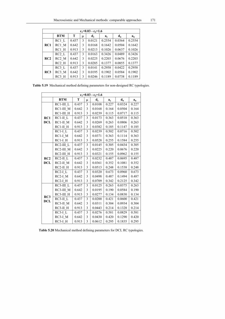
Macroseismic and Mechanical methods: comparable approaches 171
c1=0.03 - c2=1.6 BTM T µ dy ay du au
RC1_L 0.437 3 0.0121 0.2554 0.0364 0.2554 RC1_M 0.642 3 0.0168 0.1642 0.0504 0.1642 RC1 RC1_H 0.913 3 0.0213 0.1026 0.0637 0.1026 RC2_L 0.437 3 0.0163 0.3426 0.0489 0.3426 RC2_M 0.642 3 0.0225 0.2203 0.0676 0.2203 RC2 RC2_H 0.913 3 0.0285 0.1377 0.0855 0.1377 RC3_L 0.437 3 0.0141 0.2958 0.0422 0.2958 RC3_M 0.642 3 0.0195 0.1902 0.0584 0.1902 RC3 RC3_H 0.913 3 0.0246 0.1189 0.0738 0.1189
Table 5.19 Mechanical method defining parameters for non-designed RC typologies.
c1=0.03 - c2=1.6
BTM T µ dy ay du au RC1-III_L 0.437 3 0.0108 0.227 0.0324 0.227 RC1-III_M 0.642 3 0.0168 0.164 0.0504 0.164 RC1-III_H 0.913 3 0.0239 0.115 0.0717 0.115 RC1-II_L 0.437 3 0.0173 0.363 0.0518 0.363 RC1-II_M 0.642 3 0.0269 0.263 0.0806 0.263 RC1-II_H 0.913 3 0.0382 0.185 0.1147 0.185 RC1-I_L 0.437 3 0.0239 0.502 0.0716 0.502 RC1-I_M 0.642 3 0.0371 0.363 0.1114 0.363
RC1 DCL
RC1-I_H 0.913 3 0.0528 0.255 0.1584 0.255 RC2-III_L 0.437 3 0.0145 0.305 0.0434 0.305 RC2-III_M 0.642 3 0.0225 0.220 0.0676 0.220 RC2-III_H 0.913 3 0.0321 0.155 0.0962 0.155 RC2-II_L 0.437 3 0.0232 0.487 0.0695 0.487 RC2-II_M 0.642 3 0.0361 0.352 0.1081 0.352 RC2-II_H 0.913 3 0.0513 0.248 0.1538 0.248 RC2-I_L 0.437 3 0.0320 0.673 0.0960 0.673 RC2-I_M 0.642 3 0.0498 0.487 0.1494 0.487
RC2 DCL
RC2-I_H 0.913 3 0.0709 0.342 0.2125 0.342 RC3-III_L 0.437 3 0.0125 0.263 0.0375 0.263 RC3-III_M 0.642 3 0.0195 0.190 0.0584 0.190 RC3-III_H 0.913 3 0.0277 0.134 0.0830 0.134 RC3-II_L 0.437 3 0.0200 0.421 0.0600 0.421 RC3-II_M 0.642 3 0.0311 0.304 0.0934 0.304 RC3-II_H 0.913 3 0.0443 0.214 0.1328 0.214 RC3-I_L 0.437 3 0.0276 0.581 0.0829 0.581 RC3-I_M 0.642 3 0.0430 0.420 0.1290 0.420
RC3 DCL
RC3-I_H 0.913 3 0.0612 0.295 0.1835 0.295
Table 5.20 Mechanical method defining parameters for DCL RC typologies.

172 Chapter 5
c1=0.03 - c2=1.6 BTM T µ dy ay du au
RC1-III_L 0.437 3.63 0.0127 0.266 0.0459 0.266 RC1-III_M 0.642 4.11 0.0180 0.176 0.0742 0.176 RC1-III_H 0.913 4.11 0.0242 0.117 0.0995 0.117 RC1-II_L 0.437 3.63 0.0203 0.426 0.0735 0.426 RC1-II_M 0.642 4.11 0.0288 0.282 0.1187 0.282 RC1-II_H 0.913 4.11 0.0387 0.187 0.1592 0.187 RC1-I_L 0.437 3.63 0.0280 0.589 0.1015 0.589 RC1-I_M 0.642 4.11 0.0398 0.389 0.1639 0.389
RC1 DCM
RC1-I_H 0.913 4.11 0.0534 0.258 0.2199 0.258 RC2-III_L 0.437 3.19 0.0186 0.391 0.0594 0.391 RC2-III_M 0.642 3.63 0.0264 0.258 0.0959 0.258 RC2-III_H 0.913 3.63 0.0355 0.171 0.1286 0.171 RC2-II_L 0.437 3.19 0.0297 0.625 0.0950 0.625 RC2-II_M 0.642 3.63 0.0423 0.413 0.1534 0.413 RC2-II_H 0.913 3.63 0.0568 0.274 0.2058 0.274 RC2-I_L 0.437 3.19 0.0411 0.864 0.1312 0.864 RC2-I_M 0.642 3.63 0.0584 0.571 0.2119 0.571
RC2 DCM
RC2-I_H 0.913 3.63 0.0784 0.379 0.2842 0.379 RC3-III_L 0.437 3.19 0.0160 0.337 0.0513 0.337 RC3-III_M 0.642 3.63 0.0228 0.223 0.0828 0.223 RC3-III_H 0.913 3.63 0.0306 0.148 0.1110 0.148 RC3-II_L 0.437 3.19 0.0257 0.540 0.0820 0.540 RC3-II_M 0.642 3.63 0.0365 0.357 0.1324 0.357 RC3-II_H 0.913 3.63 0.0490 0.237 0.1776 0.237 RC3-I_L 0.437 3.19 0.0355 0.746 0.1133 0.746 RC3-I_M 0.642 3.63 0.0505 0.493 0.1829 0.493
RC3 DCM
RC3-I_H 0.913 3.63 0.0677 0.327 0.2454 0.327
Table 5.21 Mechanical method defining parameters for medium ductility class DCM reinforced concrete typologies derived from the Macroseimic method defining parameters
applying a [c1=0.03 - c2=1.6] I-ag law

Macroseismic and Mechanical methods: comparable approaches 173
c1=0.03 - c2=1.6 BTM T µ dy ay du au
RC1-III_L 0.437 4.67 0.0119 0.251 0.0557 0.251 RC1-III_M 0.642 5.65 0.0144 0.141 0.0814 0.141 RC1-III_H 0.913 5.65 0.0193 0.093 0.1092 0.093 RC1-II_L 0.437 4.67 0.0191 0.401 0.0890 0.401 RC1-II_M 0.642 5.65 0.0231 0.225 0.1302 0.225 RC1-II_H 0.913 5.65 0.0309 0.149 0.1747 0.149 RC1-I_L 0.437 4.67 0.0263 0.554 0.1230 0.554 RC1-I_M 0.642 5.65 0.0319 0.311 0.1799 0.311
RC1 DCH
RC1-I_H 0.913 5.65 0.0427 0.206 0.2413 0.206 RC2-III_L 0.437 4.11 0.0175 0.38 0.0719 0.368 RC2-III_M 0.642 4.97 0.0211 0.07 0.1052 0.207 RC2-III_H 0.913 4.97 0.0284 0137 0.1411 0.137 RC2-II_L 0.437 4.11 0.0280 0.588 0.1151 0.588 RC2-II_M 0.642 4.97 0.0338 0.331 0.1683 0.331 RC2-II_H 0.913 4.97 0.0454 0.219 0.2258 0.219 RC2-I_L 0.437 4.11 0.0386 0.813 0.1590 0.813 RC2-I_M 0.642 4.97 0.0467 0.457 0.2325 0.457
RC2 DCH
RC2-I_H 0.913 4.97 0.0627 0.303 0.3119 0.303 RC3-III_L 0.437 4.11 0.0151 0.317 0.0621 0.317 RC3-III_M 0.642 4.97 0.0183 0.178 0.0908 0.178 RC3-III_H 0.913 4.97 0.0245 0.118 0.1218 0.118 RC3-II_L 0.437 4.11 0.0242 0.508 0.0994 0.508 RC3-II_M 0.642 4.97 0.0292 0.286 0.1453 0.286 RC3-II_H 0.913 4.97 0.0392 0.189 0.1949 0.189 RC3-I_L 0.437 4.11 0.0334 0.702 0.1373 0.702 RC3-I_M 0.642 4.97 0.0404 0.394 0.2008 0.394
RC3 DCH
RC3-I_H 0.913 4.97 0.0541 0.261 0.2693 0.261
Table 5.22 Mechanical method defining parameters for high ductility class DCH reinforced concrete typologies derived from the Macroseimic method defining parameters applying a
[c1=0.03 - c2=1.6] I-ag law
0
1
2
3
4
5
5 6 7 8 9 10 11 12EMS-98 Intensity
µD
RC1-I_M_DCL
RC1-II_M_DCL
RC1-III_M_DCL
0
0.1
0.2
0.3
0.4
0.5
0 0.02 0.04 0.06 0.08 0.1 0.12Sd[m]
Sa[g
]
RC1-I_M_DCLRC1-II_M_DCLRC1-III_M_DCL

174 Chapter 5
0
1
2
3
4
5
5 6 7 8 9 10 11 12EMS-98 Intensity
µD
RC1-II_L_DCL
RC1-II_M_DCL
RC1-II_H_DCL
0
0.1
0.2
0.3
0.4
0.5
0 0.02 0.04 0.06 0.08 0.1 0.12Sd[m]
Sa[g
]
RC1-II_L_DCLRC1-II_M_DCLRC1-II_H_DCL
0
1
2
3
4
5
5 6 7 8 9 10 11 12EMS-98 Intensity
µDRC1-II_M_DCL
RC2-II_M_DCL
RC3-II_M_DCL
0
0.1
0.2
0.3
0.4
0.5
0 0.02 0.04 0.06 0.08 0.1 0.12Sd[m]
Sa[g
]
RC1-II_M_DCLRC2-II_M_DCLRC3-II_M_DCL
Figure 5.9 Vulnerability curves and corresponding capacity curves and for (a) RC1 medium
rise building typology considering different seismicity (b) different rise RC1 building typology for zone II (c) RC1, RC2, RC3 medium rise building typologies for zone II.
.
0
1
2
3
4
5
5 6 7 8 9 10 11 12EMS-98 Intensity
µD
RC1-III_L_DCL
RC1-III_L_DCM
RC1-III_L_DCH
0
0.1
0.2
0.3
0 0.02 0.04 0.06 0.08 0.1 0.12Sd[m]
Sa[g
]
RC1-III_L_DCLRC1-III_L_DCMRC1-III_L_DCH
0
1
2
3
4
5
5 6 7 8 9 10 11 12EMS-98 Intensity
µD
RC1-III_M_DCL
RC1-III_M_DCM
RC1-III_M_DCH
0
0.1
0.2
0.3
0 0.02 0.04 0.06 0.08 0.1 0.12Sd[m]
Sa[g
]
RC1-III_M_DCLRC1-III_M_DCMRC1-III_M_DCH

Macroseismic and Mechanical methods: comparable approaches 175
0
1
2
3
4
5
5 6 7 8 9 10 11 12EMS-98 Intensity
µD
RC1-III_H_DCL
RC1-III_H_DCM
RC1-III_H_DCH
0
0.1
0.2
0.3
0 0.02 0.04 0.06 0.08 0.1 0.12Sd[m]
Sa[g
]
RC1-III_H_DCLRC1-III_H_DCMRC1-III_H_DCH
Figure 5.10 Vulnerability curves and corresponding capacity curves and for (a) RC1 low rise building typology characterised by different ductility classes for zone III (b) RC1 medium rise
building typology characterised by different ductility classes for zone III (c) RC1 high rise building typology characterised by different ductility classes for zone III.

176 Chapter 5

Implementation of the proposed methods for seismic risk analysis 177
CHAPTER 6
IMPLEMENTATION OF THE PROPOSED METHODS FOR SEISMIC RISK
ANALYSIS
6.1. AN APPLICATION TO WESTERN LIGURIA (ITALY)
Vulnerability methods proposed in the framework of this Ph.D thesis have been operatively implemented and applied within a National and an International research project (Risk-UE research project www.risk-ue.net) related to seismic risk analysis and management. In the following the implementation steps and the results of the National research project “Earthquake scenario in Western Liguria, Italy, and strategies for the preservation of historic centres”, promoted and financed by the INGV-GNDT (National Institute of Geophysics and Vulcanology), are presented.
This experience has assembled the contributions of different scientific areas (8 research units) and the project has been split into seven tasks: seismicity and sources characterization, earthquake ground motion, site effects and interaction, assessment at sub-regional scale and vulnerability analysis, typological classification and survey of the buildings, vulnerability models and damage scenarios, traditional and innovative interventions for the damage mitigation, automatic data management.
The analysed area is characterised by a very interesting seismic history, by a complex geomorphology, by different urban tissues with historical centres and historical buildings representing a patrimony of great value to be preserved. Beyond the sub regional scale of analysis, identified with Western Liguria, an urban study case, identified with Taggia municipality, has been chosen for more detailed analysis.
The aim of the project has been the comparison and the integration of different methods, considering both the well-established and the original ones, suitable for the development, at different analysis scales, of ground shaking, vulnerability and damage scenarios.
The vulnerability methods proposed in this Ph.D thesis suit perfectly all these requirements. First of all, nevertheless being original, they maintain the compatibility with traditional methods, and allow operating with data of different origin and quality at different scales of analysis. Secondly, they permit to take into account the influence of particular soil and geomorphologic conditions on the building behaviours. Finally, thank to their analytical formulation, these methods allow an easy implementation in the GIS environment by automatic procedures.

178 Chapter 6
PIEMONTE
LOMBARDIA
LIGURIA
Ligurian See
TOSCANA
EMILIA ROMAGNA
SAVONA
LA SPEZIA
IMPERIA
GENOVA
Figure 6.1 Study area identification. The management of the project inside a GIS environment has played a leading
role, not only in order to handle and organize the acquired data and the obtained results but, above all, in order to share these among the end-users that, not necessarily belong to the scientific community. More than this, being the project multi-disciplinary, the GIS environment has made easier the communication among people belonging to different scientific areas.
For all these reasons, hazard, vulnerability, exposure and damage maps have been directly drawn on the digital cartography provided by Liguria Region; a minimum common unit of analysis has been chosen in order to be representative contemporaneously of the minimum unit of building data availability and of the territory soil characterization. The hazard evaluation has been provided applying both a deterministic and a probabilistic approach; for both the evaluations, geological and morphological information have been considered. The exposure characterizations with regard to population and building stock, has been obtained processing ISTAT census data according to a GIS automatic procedure allowing an easy updating in the case of new data availability. Overlapping hazard evaluations and vulnerability assessments, physical damage, loss and consequence scenarios have been obtained.

Implementation of the proposed methods for seismic risk analysis 179
6.2 EXPOSURE ANALYSIS: POPULATION AND BUILDING STOCK
6.2.1 Sub-regional scale data
For the sub-regional scale, population and building stock data can be derived from the ISTAT (Italian National Institute of Statistics) (1991) survey, a nation-wide census of population and dwellings carried out every 10 years.
ISTAT (1991) supplies general data about the census tract. The number of people IT living in the tract, the number of building BT, the buildings surface ST and the number of inhabited units are provided together with information about the urban zone to which the census tract belong (distinguishing between inhabited centre, inhabited nucleus and scattered houses); a census tract is classified as inhabited centre, if groups together contiguous or nearby houses (including the streets and the square along which they are built) belonging to an urban area characterized by the presence of some public service or centre. On the other hand, a census tract is reported as inhabited nucleus if it represents a group of houses, with at least five resident families, be-longing to an urban area with the absence of public services or centres. Finally, the census tract belonging to rural area is called scattered houses. Census tract general data have been graphically referred to the digital map of census tract bounds where each area is univocally identified by a unique 11 digit number (Par. 2.1.3). Figure 6.2 shows, for instance, the number of inhabitants in Western Liguria Region according to what results from ISTAT (1991).
Figure 6.2: Inhabitant number in the sub-regional area.

180 Chapter 6
In Figure 6.2 the population distribution has been represented making reference to urban areas rather then to the whole municipality area. Thus means, on respect to the distinction among urban zones operate by ISTAT, to have considered inhabited centre and the inhabited nucleus and to have neglected, in the representation, the so called scattered houses. Nevertheless urban areas represent a minor portion (and some times a very little one) of the whole municipality area, the majority of buildings and inhabitants is concentrated inside them. For this reason the representation in terms of urban areas has been preferred, resulting clearer then the one in terms of municipality areas.
Beyond general data ISTAT provides, for each census tract, statistical information on dwelling. For vulnerability purposes it is necessary to refer to buildings rather then to dwellings, therefore reference has been made to a suitable re-elaboration of ISTAT data provided by Meroni et al. (1999), over the whole national territory. Among these statistical data on buildings, homogeneous groups of buildings are identified, being characterized by a certain constructive material (masonry, reinforced concrete, pilotis, other or unknown) a certain number of floors (1 or 2 floors, from 3 to 5 floors, more than 5 floors), and a certain aggregate context (isolated or aggregate building). For each of these groups, the percentage of building, of built surface, of resident population is provided subdivided according to seven classes of age (Table 6.1). For each class of age, data about the condition of maintenance are also supplied in term of the percentage of buildings in a good state of maintenance.
Constructive
Typology Age Number of floors
Aggregate context
Maintenance conditions
Masonry
Reinforced Concrete
Pilotis
Others typologies
< 1919 1919 ÷1945 1946 ÷1960 1961 ÷1971 1972 ÷1981 > 1981
1 ÷ 2
3÷5
>6
Isolated
Aggregated
Good
Bad
Table 6.1 Information on dwelling provided by ISTAT data.
It is clear how ISTAT data are not sufficient for a direct typological identification of the buildings; therefore it has been necessary to establish inferences (Par. 2.1.2) between the building typologies and the information provided in term of the constructive material and of the class of age (Table 6.1).
In order to implement Macroseismic and Mechanical methods with the available data, 7 categories have been identified (4 for masonry building and 3 for reinforced concrete buildings) defined as shown in Table 6.2 (where building typology ad sub-typology labels are the ones adopted for the classification system in Table 2.5 and in Table 2.6 while -NC, -DCL, -DCM refer respectively to non designed building and to buildings designed according to low and moderate ductility prescriptions).

Implementation of the proposed methods for seismic risk analysis 181
Masonry Building Typology Masonry Category
M1 M3-w M3-v M3-sm M3-ca M4 M5-sm M6I M<1919 40 10 15 15 15 5 - - II M=1919 ÷ 1945 15 30 - 40 15 - - - III M =1945÷ 1971 10 10 - 10 - - 30 40 IV M> 1971 - - - 10 - - 10 80
Reinforced Concrete Building Typology Reinforced concrete
Category RC1-NC
RC1-DCL
RC1-DCM
RC1-i DCL
RC3-p DCL
RC3- DCM
RC4- DCL
RC4- DCM
V RC<1971 80 - - 10 - - 10 - VI RC=1971÷1981 - 70 - - 20 - 10 - VII RC >1981 - - 70 - 0 20 - 10
Table 6.2 Building categories identified on the basis of ISTAT data.
Inside the GIS environment, automatic procedures have been created, compiled
and run in order to process and share out ISTAT data among the building categories identified. These procedures are merely query operations, performed on respect to ISTAT constructive Typology field (Table 6.1), and sum operations of the percentages obtained for the ISTAT classes of age (Table 6.1) corresponding to the temporal intervals identifying the defined categories (Table 6.2).
ISTAT data, processed in the way above described, have been “linked” to the digital map of census tract bounds in terms of percentage of building pB,Cj, built surface pS,Cj and inhabitant pI,Cj, for each of the seven categories Cj j=I÷VII (Figure 6.3). Wanting to know the percentage of building, built surface and inhabitant for masonry (pB,M, pS,M, pI,M) and reinforced concrete building (pB,RC, pS, RC, pI,RC), it is sufficient to aggregate category percentage by sum operation respectively bounded to j=I÷IV and to j=IV÷VII as shown in equations (6.1) that make reference to the building percentage pB,CJ.
J
J
IV
B,M B,Cj I
VII
B,RC B,Cj V
p p
p p
=
=
=
=
∑
∑ (6.1)

182 Chapter 6
CERIANA
RIVA LIGURE
TAGGIA
CASTELLARO
PERINALDO
SEBORGA
OSPEDALETTI
SAN REMO
S
Edifici di categoria I[% in superficie]
75% - 100%50% - 75%25% - 50%0% - 25%
CERIANA
RIVA LIGURE
TAGGIA
CASTELLARO
PERINALDO
SEBORGA
OSPEDALETTI
SAN REMO
S
Edifici di categoria VI[% in superficie]
75% - 100%50% - 75%25% - 50%0% - 25%
Figure 6.3 Percentage of the constructive surface pS,Cj for category I (on the left) and for category IV (on the right).
For each category, building pB,Cj, built surface pS,Cj and inhabitant pI,Cj
percentages have been furthermore split, considering the percentages belonging to each class of floor number, aggregate context, maintenance conditions. Operatively this has been obtained refining furthermore the query operations, performed beyond the constructive typology, on respect to the ISTAT field’s number of floor and aggregate context (Table 6.1).
6.2.2 Local scale field survey and comparison between different origin and quality data.
For the local scale study case, identified with Taggia historical centre, population and building stock data have been collected performing a quick survey by the use of a form prepared on purpose (Balbi et al. 2004). The aim was to collect as much data as possible for the implementation of both the Mechanical and the Macroseismic approach with particular attention to catch the peculiarity of the historical centres and to the asesimic devices. Data have been geocoded by an unambiguous code to a digital map identifying (Figure 6.4) each single building together with the position of the aseismic devices and of the open space eventually available for emergency purposes.
As they are surveyed on the field with the specific aim of a vulnerability analysis, local data have been considered more reliable then the territorial one; a comparison between surveyed and ISTAT data has been performed in order to check the quality of the last ones for seismic risk analysis purposes. A good agreement between the two has been noticed with regard to the constructive typology (masonry, reinforced concrete buildings) and to the urban context characterization (isolated or aggregated buildings). On the contrary, the number of building and the built surface is underestimated for a maximum of 20%; in the same way there is about a 20% underestimation on the percentage evaluation of building in a good state of maintenance. It has been moreover noticed a 5% difference in the floor number estimation.

Implementation of the proposed methods for seismic risk analysis 183
Rud er e
Ru dere
AR
GE
NT
INA
DEGLIVIA ROMAPIAZZA
G.M
AZZ
INI
EROI TAGGIESI
RUFF
INI
MA
ZZIN
I
VIA
GIU
SE
PP
E
Cassana
Ardizzoni
VIA ROMA
Gia
rdin
o in
tern
o
inac
cess
ibile
Gia
rdin
i
Crollo
VIA
C.L.FARINI
VIA
VIA
VIAGENOVA
PARA
MURO
(S.S
.N.5
48)
PIAZZETTA
STRA
DA
VIA
GARIBALDI
Sebastiano
(GIA
' PA
NT
AN
O)
Via
Montista
EX
MU
NIC
I PIO
PA
LAZZ
OC
UR
LO
ERC
ARI
CURLO
Vi co
PIAZZA
E. Curlo
Mo lini
VIA
Vico
SO
LER
I
Lomb.di
GASTALDIP.ZA
CARD.
Salita
Anfossi
BA
ST
ION
I
Via
Nicolo'
VicoDI SAN
Via
CAVOURCHIESA
SEBASTIANOE SANFABIANO
VIA
PIAZZA
Pasqua
Via
Via Card.
Vico
GRANDEPIAZZA
S.LUCIA
PORTA
Via
PRETORIA
TAGGIA
VALLONE
P.ZADORIA
San Dalmazzo
Via
P.ZABARBARASA
Cor
tile
LuciaS.
Corti l e
Cort il e
Strad a n o n p rati c ab i le
FONTANAMEDIEVALE
STRADA
Castello
0001
00060007
1,542
9470005
Single Buildings
Census Bounds
Figure 6.4 Comparison between single building data and ISTAT data.
6.3 EARTHQUAKE HAZARD ASSESSMENT
6.3.1 Geothecnical zonation and surface morphology
With regard to the geotechnical zonation, reference has been made to the available 1:10000 geological maps. The interpretation of the near-surface formations according to a I level geotechnical zonation analysis (Par 2.2.4.1) has lead to the identification of geotechnical units, arranged by EC8 ground classes.
Ligurian See
RIVA LIGURE
CASTELLARO
CERIANA
TAGGIA
POMP
SAN REMO
Simplified Soil Classificationaccording to EC8
A: rock or very stiff groundB: Deposits of very dense sand gravel, or very stiff clayC: Deep deposits of dense or medium-dense sand, gravel or stiff clayD - Very loose deposits
Figure. 6.5 Geothecnical zonation in terms of EC8 soil classes.

184 Chapter 6
Imperia province is characterized by rugged relief, with many historical centres located on mountain or hilltops, or on steep topography, therefore an important feature in the framework of an hazard scenario assessment, has been the investigation of possible morphological amplification effects. On the basis of a DEM (Digital Elevation Map) covering the whole Imperia Province territory, the surface morphology, has been investigated and fraction of intensity degree or acceleration factors, have been attributed to 37 localities sited on markedly irregular topography (Frassine and Faccioli 2001).
Figure 6.6 DEM (Digital Elevation Model) available for Liguria Region that has lead to the identification of localities (red lines) sited on markedly irregular topography.
6.3.2 Identification of the analysis unit
In order to perform a seismic risk analysis, it has been necessary to establish how the exposure, vulnerability and hazard analysis have to interface. The chosen criterion has been to identify a minimum common unit of analysis representative contemporarily of the minimum unit of building data availability (the census tract) and of the territory soil characterization (geotechnical unit) (Balbi et al. 2004).
Therefore, the option to make reference to a mesh of regular points for the hazard assessment has been directly rejected. As a matter of fact, the hazard has to be attributed to each census tract. Making reference to a mesh of regular points, an average operation would have been necessary, both in the case of more then one point corresponding to the tract and in the case no points are identified in the tract. On the basis of these considerations, the decision to maintain the original repartition of the territory into census tracts and to make reference to the mesh of census tract centroid could represent a suitable solution. In this way, for each census tract, a point for the hazard evaluation is defined, and it is unique. This solution does not allow, anyway, to represent in a suitable way soil conditions that could be different

Implementation of the proposed methods for seismic risk analysis 185
inside the same census tract area. In order to overcome this limitation, making reference to the simplified geotechnical zonation, each census tract has been split into portions corresponding to different soil categories identified inside the census tract.
Figure 6.7 represents a zoom of Figure 6.5 where it is shown how 0028 census tracts has been split in 5 portions (analysis units) in order to take into account the non-homogeneous soil conditions inside the tract.
TAGGIA
Ligurian SeeSAN REMO
0028
0026
0025
0021
0020
0019
0022
00280028
0028
0028
Figure 6.7 Identification of the analysis unit. This operation has been easily performed by the use of spatial analysis in the GIS
environment that allows queering and searching operations based on the geographic concepts of belonging, containing, intersecting and adjoining.
In essence, the hazard has been evaluated making reference to the mesh of the centroids of these census tract portions. The exposure and the vulnerability characterization of these portions have been obtained disaggregating ISTAT data referred to the census tract. The same general data characterizing the census tract have been directly attributed to its portions (ISTAT code, name of the municipality and locality to which the tract belong) while, with regard to the information about inhabitant and buildings, a weighted repartition on the basis of the surface of each portions has been performed. In order to take into account soil amplification effects according to both the procedure presented (Mechanical and Macroseismic method) the soil category, attributed in the framework of the geotechnical zonation analysis, has been automatically attributed to each census tract portion and to each centroid.
6.3.3 Deterministic seismic hazard scenarios
The identification of the scenario earthquakes has been performed considering the

186 Chapter 6
main historical earthquakes (Guidoboni 2001), the recorded instrumental seismicity and considering the seismogenetic sources (Eva et al. 2000) identified inland and along the border of the Liguria Sea. Two reference earthquakes have been selected: a catastrophic event, identified with 1887 (February 23) Western Liguria earthquake, and a moderate historical event, identified with the inland May 1831 M5.5 event.
In particular, 1887 Western Ligurian earthquake represents, with an estimated 6.3 Magnitude, the maximum historical. It caused over 509 victims, severe destruction in costal towns, such as Porto Maurizio, and villages (Diano Castello, with the maximun intensity X MCS) as well as damaging effects over a wide area; in France, Menton and Nice experienced rescpectively VII-VIII and VII MCS (Taramalli et al. 1888).
Having identified the position of the earthquake scenario epicentres (in term of longitude and latitude as in Table 6.3), deterministic hazard scenarios have been automatically implemented in the GIS environment, evaluating the source-site distance, (distance between the epicentre of the scenario earthquake and each of this centroid) required by the selected predictive equation by a GIS function.
For macroseimic intensity scenarios, Howell and Shcultz (1975) attenuation law has been employed (6.2), whose parameters have been properly calibrated on the basis of the comparison with the known resentments (Table 6.3).
0I I a b ln(D) c D− = + ⋅ + ⋅ (6.2)
I0 [EMS-98] M Longitude Latitude a b c 1887 X 6.3 8°,1430 43°,7480 -1.6017 1.3092 -0.00631831 VIII 5.5 7°,8594 43°,8627 -1.6017 1.0258 0.0660
Table 6.3 Magnitude, macroseismic Intensity epicenter position for the assumed scenario
earthquakes and parameters defining the assumed attenuation law. Macroseismic intensity hazard assessment have been developed both for the two
scenario earthquakes; Figure 6.8 shows in particular the case of 1887 earthquake.

Implementation of the proposed methods for seismic risk analysis 187
Figure 6.8 Macroseismic intensity deterministic hazard scenario for the 1887 earthquake. PGA hazard scenarios have been drawn making reference to AMB96 predictive
equation (2.15). According to this equation, the site-source distance is defined as the shortest distance between the site and the surface projection of the source identified for 1831 as a L=1 km linear source on Sourge-Taggia fault.
Figure 6.9 PGA deterministic hazard scenario for the 1831 earthquake.

188 Chapter 6
6.4 VULNERABILITY ASSESSEMNT AND PHYSICAL DAMAGE EVALUATION
6.4.1 Implementation of the Macroseismic method
According to the Macroseimic method the vulnerability index for building categories can be defined as:
j 0 j
CC C k m k
k
V V r V= +∑ , (6.3)
where
0 jCV is the most probable vulnerability index for the j-category, rC,k e Vm,k
are respectively the percentage and the score of the k-behaviour modifier affecting the
jCV category.
The most probable vulnerability index for each j-category 0 jCV has been
attributed combining the basic vulnerability index V0 of the building typologies according to the inference percentages as explained in Par 3.7.2. In particular, the resulting
0 jCV for the inferences assumed in the case of Western Liguria Region
(Table 6.2), are shown in Table 6.4.
Masonry Categories VC R.C Categories VC I M<1919 0.79 V RC<1971 0.59 II M=1919 ÷ 1945 0.73 VI RC=1971 ÷ 1981 0.55 III M =1945 1971 0.69 VII RC >1981 0.42 IV M> 1971 0.65
Table 6.4 Most probable vulnerability index values for the seven categories identified in
Western Liguria Region. The behavior modifier parameters that can be identified by ISTAT data (Table
6.1) are the number of floor, the aggregate context and the maintenance conditions. Scores Vm,k have been attributed to these behavior modifier parameters (Frassine and Giovinazzi 2004) according to the proposal shown in Table 3.5 and according to the further considerations made after the calibration and comparison with the mechanical method (Chapter 5).
For each analysis unit (i-portion of the census tract) VUi, the vulnerability index of the seven building categories
0 jCV (j=I÷VII) identified, has been evaluated
combining the vulnerability index according to the percentage of building pB,Cj, building surface pS,Cj, and inhabitants pI,Cj belonging to each j-category, evaluated by the exposure analysis (Par. 6.3).
Formula 6.4 shows the evaluation of VUi in the case reference is made to all kind of building typologies and to the percentage of the building surface pS,CJ. Wanting to

Implementation of the proposed methods for seismic risk analysis 189
evaluate VUi separately for masonry and reinforced concrete buildings, the sum operation in (6.4) have to be bounded respectively to j=I÷IV and to j=IV÷VII.
Cj
VII
Ui S Cjj I
V p V=
= ∑ (6.4)
Finally, the vulnerability index for the whole census tract VT has been obtained
aggregating the results obtained in terms of iUV for each of the i-analysis units
belonging to the census tract:
iT i U
iV a V= ∑ (6.5)
The operations (6.3), (6.4) and (6.5), leading to the census tract vulnerability
index evaluation have been performed automatically in the GIS environment by procedures created on purpose.
Figure 6.10 show a representation of the vulnerability index evaluated for each census tract VT for masonry (left) and for reinforced concrete buildings (right).
Figure 6.10 Census tract vulnerability index evaluation VT for masonry (left) and reinforced concrete buildings (right). The representation is in terms of the vulnerability index ranges
corresponding to the vulnerability classes (Table 3.3).

190 Chapter 6
Figure 6.11 Census tract vulnerability index evaluation VT for all kind of building. The representation is in terms of vulnerability index ranges corresponding to the vulnerability
classes (Table 3.3) and is aggregated for urban areas. Once the vulnerability index representative of the census tract has been evaluated
(for all the building typologies or separately for masonry and reinforced concrete buildings), the estimation of the corresponding mean damage grade and damage distributions has been a straightforward operation performed by automatic procedure implementing equations (3.11) and (3.8). This has lead to the final estimation, for the building-stock belonging to the tract, of the probability to suffer a k-damage Pk,T (k=1÷5 according to the assumed damage scale in Table 2.17).
Figure 6.12 Vulnerability index V for each single building of Taggia historical centre.

Implementation of the proposed methods for seismic risk analysis 191
6.4.2 Implementation of the Mechanical method
At sub-regional scale, the implementation of the Mechanical method have to refer as well, to ISTAT data, that provide a characterization of the built environment in terms of building categories rather then of building typologies.
However, the definition of a bilinear capacity curve for a building category is of a little point, as there is no physical sense in defining mechanical parameters for a distribution of different building typologies. For this reason some preliminary evaluations have to be performed independently from the consistency of the building stock inside the census tract. For each analysis unit, it is necessary to evaluate the performance point (4.42), considering soil condition and the hazard value, for all the typologies defining building categories, according to the inferences assumed (Table 6.2). After that, for each typology, the evaluation of the damage distribution pk (k= 1÷5) is performed (Par. 4.7).
For each of the seven building categories Cj j=I÷VII defined in Table 6.2, the damage distribution is, thus, evaluated as the weighted average of the damage distributions got for the building typologies to which reference is made in defining the inferences.
k Cj t k tt
p r p= ∑, , (6.6)
where rt is the percentage of the t-typology inside the j-category according to
the assumed inference and pkt is the probability for the t-typology to suffer a k-damage.
For each analysis unit (k-portion of the census tract) pk,Ui, the damage distribution has been evaluated combining the damage distribution for the seven building categories identified pk,Cj according to the percentage of the buildings pB,Cj, of the building surfaces pS,Cj, and of the inhabitants pI,Cj belonging to each j-category, evaluated by the exposure analysis (Par. 6.3).
Formula 6.6 shows the evaluation of pk,Ui in the case reference is made to the percentage of the building surface pB,Cj and to all kind of buildings. Wanting to evaluate VUi separately for masonry and reinforced concrete buildings, the sum operation in (6.7) have to be bounded respectively to j=I÷IV and to j=IV÷VII.
k Ui S Cj k Cjj
p p p= ∑, , , (6.7)
Finally the damage distribution for the whole census tract pk,T is obtained
aggregating the results obtained in term of pk,Ui for each of the i-analysis units belonging to tract. k T i k Ui
i
p a p= ∑, , (6.8)

192 Chapter 6
6.5 DAMAGE AND CONSEQUENCE SCENARIOS
Damage and consequences scenarios have been evaluated making reference to the results provided on one hand by the exposure analysis, in terms of the percentage of buildings, built surface, inhabitants for each category or for masonry or reinforced concrete buildings (pB,Cj, pS,Cj , pI,Cj,; pB,M , pS,M , pI,M; pB,RC , pS, RC , pI, RC) and, on the other hand, by the results obteined in terms of damage probability distribution pk,T (k=1÷5) crossing the hazard and the vulnerability analysis. The statistical correlations employed for the evaluation of the consequences on buildings and on people are the one provided by SSN (Bramerini 1995) as from the analysis made in Par. 2.4 they result to be intermediate between the other proposals. Formulas from (6.9) to (6.12) show the implementation of these correlations in the case reference is made to masonry buildings. It is worth noting that, for the evaluation of the consequence on buildings, reference has been made to the results provided by the exposure analysis in terms of building percentage pB,M and, on the other hand, reference has been made to the inhabitants percentage pI,M dealing with the evaluation of the consequences on people (for loss evaluations that are not reported here, the built surface percenatge has been used pS,M).
The number of collapsed buildings N5,M and the number of uninhabitable dwelling NUf,M have been evaluated as follow:
5 M T B M 5 TN B p p=, , , (6.9) ( )Ud M T B M 3 T 4 T 5 TN B p 0 4p p p= + +, , , , ,. (6.10)
The number of dead people NS4,M and the number of people needing a temporary
shelter (as previously leaving in unfit for use buildings) NI,Uf,M have been evaluated as follow:
S4 M T I M 5 TN B p p=, , , (6.11) ( )I Ud M T I M 3 T 4 T 5 TN B p 0 4p p p= + +, , , , , ,. (6.12)
As reference is made to data provided by the population census (ISTAT 1999),
the estimation of casualties is given in the hypothesis that the earthquake occurs during nighttime.
Table 6.5 and Table 6.6 show the results obtained for the 1887 earthqauke scenario applying, respectively, the Macroseimic and the Mechanical approach.

Implementation of the proposed methods for seismic risk analysis 193
1887 - Macroseimic CONSEQUENCES ON BUILDINGS Masonry R.C. All % Unfit for use building 3775 563 4337 8.8 Collapsed Building 208 15 223 0.5
CONSEQUENCES ON PEOPLE Masonry R.C. All % People requiring short term shelter 10317 6700 17017 8.1 Dead and severely injured people 182 71 253 0.1
Table 6.5 1887 damage scenario implementing Macroseismic approach.
1887 - Mechanical CONSEQUENCES ON BUILDINGS Masonry R.C. All % Unfit for use building 4706 1102 5808 11.8 Collapsed Building 530 69 599 1.2
CONSEQUENCES ON PEOPLE Masonry R.c. All % People requiring short term shelter 14150 11327 25477 12.1 Dead and severely injured people 552 249 801 0.4
Table 6.6 1887 damage scenario implementing Mechanical approach.
The reliability of the results has been verified by the comparison with real data,
available from 1887 earthquake (Calvini 1987). The 23 February 1887 earthquake caused 509 dead over a population of 49.000 people (corresponding to about the 1% of the whole population). It must be considered, anyway, that 212 people dead because of the roof collapse of the church in Baiardo.
In order to compare the results with the ones obtained from the risk analysis, these people have not to be considered as the proposed damage scenario procedures do not take into consideration special building typologies subjected to high crowding. The percentage of dead people obtained in this case is equal to 0.6% of the whole population.
On the other hand, with regard to the results obtained implementing the risk analysis, reference has to be made to the percentage of people dead in masonry buildings (Table 6.7 shows the number of inhabitants living in masonry buildings) thus considering that in 1887 all the built-up environment was made of masonry buildings. A percentage of dead equal to 0.2% results if reference is made to the Macroseismic scenario (Table 6.5) and a percentage equal to 0.65% (Table 6.6) outcomes if reference is made to the Mechanical scenario. It is therefore possible to conclude that these results are definitely coherent with what observed after 1887 earthquake.

194 Chapter 6
Number Percentage All R.C. Masonry R.C. M Number of Buildings 49372 17733 31639 36% 64% Number of Hinabitants 211349 126616 84733 60% 40%
Table 6.7 Information on dwelling provided by ISTAT Data
Figure 6.13 shows the evaluation of dead/ km2 (left) and of collapsed building/
km2 (right) for each census tract of Imperia municipality. It is worth noticing the value of such a detailed representation for the immediate post emergency period to have an idea where to concentrate resque teams or which could be the streets prone to obstruction because of collapsed buildings.
Figure 6.13 Dead people/km2 (left) and collapsed building/km2 (right) for Imperia
municipality according to 1887 macroseismic scenario. Table 6.8 and Table 6.9 show the results obtained for the 1831 earthquake
scenario respectively applying the Macroseimic and the Mechanical approach. The results provided by the simulation of an “ordinary” earthquake and a
representation of the results in terms of urban area on the whole sub-regioonal territory could provide a useful support for checking the availability of the resources on respect to sheltered population and people needing medical aid.
1831 - Macroseimic CONSEQUENCES ON BUILDINGS Masonry R.c. All % Unfit for use building 845 102 947 1.9 Collapsed Building 58 3 61 0.1
CONSEQUENCES ON PEOPLE Masonry R.c. All % People requiring short term shelter 2509 1515 4024 1.9 Dead and severely injured people 52 16 68 0.03
Table 6.8 1831 Macroseismic approach damage scenario

Implementation of the proposed methods for seismic risk analysis 195
1831 - Mechanical CONSEQUENCES ON BUILDINGS Masonry R.c. All % Unfit for use building 1879 160 2040 4.1 Collapsed Building 127 4 131 0.3
CONSEQUENCES ON PEOPLE Masonry R.c. All % People requiring short term shelter 5375 1494 6869 3.3 Dead and severely injured people 118 14 131 0.1
Table 6.9 1831 Mechanical approach damage scenario
Figure 6.14 Dead people (left) and people needing temporary shelters (right) for Western Liguria territory according to 1831 macroseimic scenario.
The results of INGV-GNDT Western Liguria project are available, for
consultation at http://adic.diseg.unige.it/gndt-liguria.

196 Chapter 6

Conclusions and future research 197
CHAPTER 7
CONCLUSIONS AND FUTURE RESERCH
In this Ph.D thesis the proposal of two seismic vulnerability methods has been addressed with the main objective of their implementation in the framework of a seismic risk analysis, in order to draw damage and consequence scenarios for risk mitigation and risk management purposes.
A Macroseismic method has been defined to be used for macroseismic intensity hazard descriptions; on the other hand, a Mechanical-based method has been proposed to be applied when the hazard analysis is provided in terms of peak ground accelerations or spectral accelerations. For both the methods ground motion amplifications, due to particular soil conditions, have been accounted in a coherent way and considering the dynamic characteristics of the built environment.
The procedure for the exposure analysis for the built-environment, finalized to the vulnerability methods implementation, has been described, showing how both the methods can be employed either with properly surveyed data or with existent data of different origin and quality.
Thus, the procedures to be followed for the evaluation of damage distributions and of loss and consequence fragility curves have been presented. A way to differently characterize the uncertainty on the final damage estimations, depending on the quantity and on the quality of the available data, has been proposed. Finally, the two methods have been compared and, since they have shown to provide comparable results, they have been reciprocally tuned and calibrated leading to the definition of a Macroseimic and Mechanical methods providing equivalent results in terms of damage scenarios when implemented on respect to coherent hazard descriptions.
Automatic procedures have been developed in order to implement the proposed vulnerability methods and their interaction with hazard and exposure analysis, in a GIS environment that allow drawing thematic map for the estimated damage scenarios. The GIS implementation of the proposed methods has been presented for the Western Liguria Region.
The results obtained implementing the proposed vulnerability models and the risk analysis procedures become effective tools for risk mitigation and for risk management purposes.
Land use planning controls and planning regulations can be drawn from the proposed seismic risk analysis procedures, as they help identifying parts of a city or of a region where earthquake risk is higher, either because of the hazard or because of the exposure or of the building vulnerability.

198 Chapter 7
Risk analysis results can be processed in order to obtain useful guidance in establishing structural protection measures i.e. the retrofitting of the existing building stock planning effective strengthening programmes. As a matter of fact, the building typologies and the urban areas needing more protection can be recognized thanks to vulnerability analysis. Drawing different damage scenarios, the easiest and cheapest reduction strategies can be identified and their effectiveness can be tested.
The value of having a versatile GIS system for preparedness plans is unquestionable. First of all, important data, such as building damage, sheltered population and people needing aid can be evaluated and displayed graphically using the GIS system. This information, when combined with a listing of resources, allowed a more effective match of need versus resources and provides a support to decide about resource allocation. Secondly, from deterministic hazard scenarios it is possible to single out the areas possibly more affected and the street more prone to obstruction, on the basis of which it is possible to decide the routing to use in case of emergency (escape streets) and to identify safe spaces. Finally, the availability of maps easy to read can help to share the knowledge about the proper behaviour to assume in the event of an emergency and to increase the public awareness about the danger they are subjected to.
The real possibility to employ the proposed methods for insurance and reinsurance industry (whose role in risk mitigation is to finance the losses undertaken by the private and by the public sector after an earthquake occurrence) has been also verified thanks to a training period spent in the Munich-RE Reinsurance Company, in the framework of this Ph.D thesis. As a matter of fact, given the lack of historical data required to perform statistical analysis on insurance claims, insurers are increasingly relying on the engineering community for catastrophe loss modelling. Earthquake damage prediction provided by the proposed vulnerability models, in conjunction with the seismic hazard assessment, have been employed for determining premium rates that, taking into account, different factors which affects the damage potential, reflect adequately the risk underwritten.
Finally, the chance of having loss estimations in the critical minutes and hours following a major damaging earthquake can be regarded as a key result of this work. Making reference to the proposed procedures, the only input information required for the users to generate damage scenarios are, indeed, the earthquake magnitude and the epicentre location immediately available from the worldwide seismometer networks. It is worth noticing that the whole procedure for damage scenario evaluation runs automatically on a computer provided with a GIS program. The development, for the Civil Protection Department of Liguria Region, of a tool for the implementation of real–time damage scenarios, applying the vulnerability methods and the procedures defined in the framework of this thesis is in progress.
One aspect that remain to be investigated and that it is proposed for future researches is the improvement of the proposed methods for the application on single building. Nevertheless the proposed vulnerability methods can be employed for different scale of analysis, both the vulnerability and the ductility indexes defying

Conclusions and future research 199
the proposed Macroseimic approach, and the capacity curve parameters defying the proposed Mechanical approach, have been evaluated in such a way to be representative, on average, of the characteristic behaviour of building typologies. For this reason, it is misleading to believe that the vulnerability assessment and the consequent damage estimation for a single building is representative of its real structural response to an earthquake. More likely, it can be considered representative of the behaviour of the building typology to which the single building belongs to.
The future research is addressed, therefore, to the identifications and to the inclusion on the proposed vulnerability methods, of the mechanical and structural parameters able to provide a more reliable representation of the single building vulnerability.

200 Chapter 7

I
REFERENCES
Alexander D. (1996). The health effects of earthquake in the mid-1990’s. Disaster, 30(3), pp.231-247.
Ambraseys N.N., Simpson K.A., Bommer J.J. (1996). Prediction of horizontal response spectra in Europe. Earthquake Engineering and Structural Dynamics, 25, pp. 371-400.
Arioglu E. and Anadol K. (1973). The structural performance of rural dwellings during recent destructive earthquakes in Turkey (1969-1972). Proc. of 5th World Conference on Earthquake Engineering, Rome, Italy.
Arioglu E. and Anadol K. (1977). Response of rural dwellings to recent destructive earthquakes in Turkey (1973-1975). Proc. of 6th World Conference on Earthquake Engineering, Sarita Prakashan, Meerut, India, Vol. I, pp. 249-254.
ATC 13 (1987). Earthquake damage evaluation data for California. Applied Technology Council, Redwood City, California.
ATC 21 (1988). Rapid Visual Sreening of building for Potential Seismic Hazards: a Handbook. Applied Technology Council, FEMA-145, Redwood City, California.
ATC 40 (1996). Seismic evaluation and retrofit of concrete buildings. Applied Technology Council, Redwood City, California.
ATC (2002). Summary of evaluation of current nonlinear static procedures-SDOF studios. Report ATC-55 Applied Technology Council, Redwood City, California.
Avorio A. and Borri A. (1997). Rischio sismico del bene culturale “centro storico” proposta per una catalogazione ed analisi. Proc. of 8th Italian Conference on Earthquake Engineering, Taormina, Italia.
Ayyub B.M. and Chao R. J. (1998). Uncertainty Modelling in Civil Engineering with structural and reliability Application. Uncertainty Modelling and Analysis in Civil Engineerin. CRC Press, Boca Raton, Usa, pp. 3-32.
Balbi A., Giovinazzi S., Lagomarsino S. (2004). A vulnerability method for historical centre buildings. Proc. of 11th Italian Conference on Earthquake Engineering, Genoa, Italy.
Balbi A., Cortellesi D., De Luigi G., Eva C., Giovinazzi S., Spallarossa D., Lagomarsino S., Ugolini P. (2004). Prevention and management of seismic risk in Liguria. Proc. of 11th Italian Conference on Earthquake Engineering, Genoa, Italy.

II
Bard (1998). SERINA: Seismic Risk and Integrated Seismological, Geothecnical and Structural Approaches. ITSAK, European Commission, Directorate General for Science and Development.
Bender and Perkins (1987). SEISRISK III: a Computer Program for seismic Hazard Estimation. USGS bulletin 1772.
Benedetti D. and Petrini V. (1984). On seismic vulnerability of masonry buildings: proposal of an evaluation procedure. The industry of constructions, Vol. 18, pp. 66-78.
Bernardini, A. (1997). Coherence between observations and forecasts of seismic vulnerability of masonry typologies Proc. of 11th Italian Conference on Earthquake Engineering, Taormina, Italy, pp. 177-183.
Bernardini, A. (1999). Seismic Damage to Masonry Buildings. Proc. of the Int. Workshop of Seismic Damage to Masonry Buildings, Monselice, Padua.
Bernardini, A. (2000). The vulnerability of buildings – Evaluation on a national scale of the seismic vulnerability of ordinary building, CNR-GNDT, Rome.
Bommer J. J. (2002). Deterministic versus Probabilistic seismic hazard assessment: an exaggereted and obstructive dichotomy. Journal of Earthquake Engineering, Vol. 6, Special Issue 1, pp.171-199. Imperial College Press.
Braga F., Dolce M., Liberatore D. (1982). A statistical study on damaged buildings and an ensuing review of the M.S.K76 scale. Proc. of the 7th European Conference on Earthquake Engineering, Athens.
Bramerini F., Di Pasquale G., Orsini A., Pugliese A., Romeo R., Sabetta F., (1995). Rischio sismico del territorio italiano. Proposta per una metodologia e risultati preliminari. Rapporto tecnico del Servizio Sismico Nazionale SSN/RT/95/01, Roma (In Italian).
Calvi G.M. (1999). A displacement-based approach for vulnerability evaluation of classes of buildings, Journal of Earthquake Engineering, 3, 3, pp. 411-438.
Calvino N. (1987). Il terremoto del 23 febbraio 1887 nel ponente Ligure. Edizioni Dominaci, Oneglia, Imperia.
Cattari S., Curti E., Giovinazzi S., Lagomarsino S., Parodi S., Penna A, (2004). A mechanical model for the vulnerability assessment and the damage scenario of masonry buildings at urban scale. Proc. of 11th Italian Conference on Earthquake Engineering, Genoa, Italy.
CEN (Comité Europeén de Normalisation), (2003), prEN 1998-1-Eurocode 8: Design of Structures for earthquake resistance. Part 1: General rules, seismic actions and rules for buildings. Pr-EN 1998-1. Draft N°6, Doc CEN/TC250/SC8/N335, January 2003, Brussels.

III
Chopra A.K. and Goel R.K. (1999). Capacity-Demand-Diagram methods based on inelastic spectrum, Earthquake Spectra, 15, 4, pp. 637-656.
Coburn A. and Spence R. (1992-A). Earthquake Protection. John Wiley & Sons Ltd., Chichester, England.
Coburn A. and Spence R. (1992-B). Factors Determining Human Casualty Levels in Earthquakes: Mortality Prediction in Building Collapse. Proc. of the 10th World Conference on Earthquake Engineering, Madrid, Spain, pp. 5989-5994.
Coburn, A. and Spence R. (2002). Earthquake Protection (Second Edition), John Wiley and Sons Ltd., Chichester, England.
Cornell C. A. (1968). Engineering Seismic Risk Analysis. Bulletin of Seismological Society of America, Vol.58, No5, pp.1583-1606.
Corsanego A and Petrini V. (1994). Evaluation criteria of seismic vulnerability of the existing building patrimony on the national territory. Seismic Engineering, Patron ed., Vol. 1, pp. 16-24.
Crespellani T., Vannucchi G., Zeng X., (1992). Seismic Hazard Analysis in the Florence Area. European Earthquake Engineering, 3.
Crespellani T., Madiai C., Marcellini A., Maugeri M., Vannucchi G., (1997). Zonation of geothecnical seismic hazards in Tuscany, Italy in Seismic Behaviour of Ground and Geotechnical Structures, Seco and Pinto P. S. Edition.
D’Ayala D. and Speranza E. (2003). Definition of Collapse Mechanisms and Seismic Vulnerability of Masonry Structures, Earthquake Spectra, 19(3), pp.479-509.
Dolce M., Zuccaro G., Kappos A., Coburn A. (1994). Report of the EAEE Working Group 3: Vulnerability and risk analysis. Proc. of 10th European Conference on Earthquake Engineering, Vienna, Vol. 4, pp. 3049-3077.
Dong W., Shah H., Wong F. Expert System in Construction and Structural Engineering. New York: Chapman and Hall, London, 1988.
Dubois D. and Parade H (1980). Fuzzy Sets and Systems. Academic Press, New York.
Durkin M. E., and Thiel C. C. (1993). Towards a Comprehensive Regional Earthquake Casualty Modeling Process. Proc. of National Earthquake Conference. Vol I, Central U.S. Earthquake Consortium, pp. 557-566.
Eva C., Augilera P., Eva E., Solarino S., Spallarossa D. (2000). Sintesi delle conoscenze sulla sismotettonica della Liguria Occidentale ed influenza sui parametri di Hazard. In: Galadini F., Meletti C., Rebez A (Editors). Le ricerche del GNDT nel campo della pericolosità sismica (1996-1999), CNR - Gruppo Nazionale per la

IV
Difesa dei Terremoti, Roma, pp. 59-70.
Everdnden J., Hibbard R., Schneider J. (1973). Interpretation of Seismic Intensity data. Bulletin of Seismological Society of America, Vol.63.
Everdnden J., Thomson J.M., (1985). Predicting Seismic Intensities. U.S. Geol. Survey. Profes. Paper 1360.
Faccioli E. (1991). Seismic amplification in the presence of geological and topographic irregularities. Proc. of the 2nd International Conference on Recent Advences in Geotechnical earthquake Engineering and Soil Dynamics, St. Louis, USA, pp: 1779-1797.
Faccioli E., Vanini M., Frassine L. (2002). “Complex” site effects in earthquake round motion, includine topography. Proc. of 12th European Conference on Earthquake Engineering, London.
Faccioli E. and Pessina V. (2003). WP2-Basis of an handbook of earthquake ground motion scenarios. Risk-UE Project: An advanced approach to earthquake risk scenarios with applications. http://www.risk-ue.net.
Fajfar P. (1999). Capacity spectrum method based on inelastic demand spectra, Earthquake Engineering and Structural Dynamics, 28, pp. 979-993.
Fajfar P. (2000). A non linear analysis method for performance-based seismic design, Earthquake Spectra, 16, 3, pp. 573-591.
Farsi M. N. and Belazougui M. (1992). The Mont Chenoua (Algeria) earthquake of October 29th, 1989: damage assessment and distribution. Proc. of 10th World Conference on Earthquake Engineering, Vol. 1, pp. 11-13.
FEMA 154 (1988). Rapid Visual Screening of Buildings for Potential seismic Hazards: Supporting Documentation. FEMA, Washington.
Frassine L. and Faccioli E., (2001). Effetti della localizzazione sfavorevole di centri abitati sulla distribuzione regionale dello scuotimento: indagini preliminari sul terremoto ligure del 1887. Proc. of 10th Italian Conference on Earthquake Engineering. Potenza, Italy (in Italian).
Frassine L. and Giovinazzi S. (2004). Seismic vulnerability of ordinary buildings: an application to Catania town with different databases. Proc. of 11th Italian Conference on Earthquake Engineering,. Genoa, Italy.
Freeman S.A., Nicoletti J.P., Tyrell J.V. (1975). Evaluation of existing buildings for seismic risk - A case study of Puget Sound Naval Shipyard, Bremerton, Washington, Proc. of the U.S.National Conference on Earthquake Engineers, EERI,113-122, Berkeley.
Freeman S.A. (1998). The Capacity Spectrum Method. Proc. of 11th European

V
Conference on Earthquake Engineering, Paris.
Freeman S.A. (2004). Why properly code designed and costructed buildings have survived major erthquakes. Proc. of 13th 10th World Conference on Earthquake Engineering. Vancouver, Canada.
Giovinazzi S. and Lagomarsino S (2001). Una metodologia per l’analisi di vulnerabilità sismica del costruito Proc. of 10th Italian Conference on Earthquake Engineering, Potenza, Italy (in Italian).
Giovinazzi S. and Lagomarsino S. (2003). Seismic Risk Analysis: a method for the vulnerability assessment of built-up areas. European Safety and Reliability Conference ESREL, Maastricht, The Netherlands.
Giovinazzi S. and Lagomarsino S. (2004). A Macroseismic Model for the vulnerability assessment of buildings. 13th World Conference on Earthquake Engineering. Vancouver, Canada.
Giuffrè A. (1993). Sicurezza e conservazione dei centri storici: il caso di Ortigia, Laterza Editions, Bari.
GNDT, 1994. Scheda di esposizione e vulnerabilità e di rilevamento danni di primo livello e secondo livello (muratura e cemento armato). Gruppo Nazionale per la Difesa dai Terremoti, Roma (in Italian).
Grandori G., Drei F., Perotti F., Tagliani A. (1991). Macroseismic intensity versus epicentral distance: the case of central Italy. Tectonophysics, 193, pp. 165-17.
Grunthal G. (1998). European Macroseismic Scale. Centre Européen de Géodynamique et de Séismologie, Luxembourg. Vol. 15.
Guagenti E., Petrini V. (1989). Il caso delle vecchie costruzioni: verso una nuova legge danni-intensità. Proc. of 4th Italian Conference on Earthquake Engineering, Milano, Vol. I, pp. 145-153.
Guerrieri F. (edited by) (1999). Manuale per la riabilitazione e la ricostruzione postsismica degli edifici. Roma. DEI.
Guidoboni E. (2001), Personal comunication of GIS files.
HAZUS (1999). Earthquake Loss Estimation Methodology - Technical and User Manuals. Federal Emergency Management Agency, Washington, D.C.
Howell B.F. and Schultz T.R. (1975). Attenuation of modified Mercalli intensity with distance from epicenter. Bulletin of Seismological Society of America, 65, pp. 651-665.
ISTAT 1991. 13th General Census of the Population 1991 - Data on the structural characteristics, of the population and housing. Rome.

VI
Jibson R. (1987). Summary of research on the effects of topographic amplification of earthquake shaking on slope stability. Open-File – Report 87-268, U.S. Geological Survey, Menlo Park, California.
Jones N. P., Noji E. K, Smith G.S., Wagner R.M., (1993). Casualty in earthquakes. National Earthquake Conference, Central United States Earthquake Consortium. Memphis, TN, May 2-5. Monograph 5: Socioeconomic Impacts, Chapter 5, pp. 19-53.
Kappos A., Pitilakis K., Stylianidis K. and Morfidis K. (1995). Cost-benefit analysis for the seismic rehabilitation of buildings in Thessaloniki, based on a hybrid method of vulnerability assessment. Proc of the 5th International Conference on Seismic Zonation, Nice, Vol. 1, pp. 406-413.
Karaesmen E. (1973). Observations on the behaviour of reinforced concrete framed buildings during 22 May 1971 Bingol earthquake. Proc. of 5th World Conference on Earthquake Engineering, Rome, Italy.
Kircher C. A., Nassar A.A., Kuster O., Holmes W.T. (1997). Development of building damage functions for earthquake loss estimation. Earthquake Spectra, 13(4), pp. 663-682.
Kramer S.L. (1996). Geothecnical Earthquake Engineering, Prentice Hall.
Lagomarsino S. and Podestà S. (2004a). Seismic vulnerability of ancient churches. Part 1: damage assessment and emergency planning. Earthquake Spectra, 20(2), pp. 377-394.
Lagomarsino S. and Podestà S. (2004b). Seismic vulnerability of ancient churches. Part 2: statistical analysis of surveyed data and methods for risk analysis. Earthquake Spectra, 20(2), pp. 395-412.
Lagomarsino S. and Podestà S. (2004c). Damage and vulnerability assessment of
churches after the 2002 Molise, Italy, earthquake. Earthquake Spectra, 20(S1), pp. S271-S283.
Lungu D., Aldea A., Arion A., Vacareanu R., Petrescu F., Cornea T. (2001). WP1 Report European distinctive features, inventory database and typology. Risk-UE Project: an advanced approach to earthquake risk scenarios with applications. http://www.risk-ue.net.
Margottini C., Molin D., Narcisi B., Serva L., (1992). Intensity versus ground motion: a new approach using Italian data. Engineering Geology, 33, pp. 45-48.
McCormack T. and Rad F. N. (1997). An Earthquake Loss Estimation Methodology for building Based on ATC-13 and ATC-21. Earthquake Spectra, Vol. 13(4).
McGuire R. K. (1976). FORTRAN computer program for seismic risk analysis.

VII
US Geological Survey open file report pp. 67-76.
McGuire R. K. (2004). Seismic Hazard and risk analysis. EERI Earthquake Engineering research Institute.
Medvedev (1977). Seismic Intensity Scale M.S.K.-76. Publ. Inst. Geophys. Pol. Acad. Sc. Warsaw, A-6 (117).
Medvedev J. (1962). Engineering Seismology. Academia Nauk Press. Moscow.
Meroni F., Petrini V. and Zonno G. (1999). Evaluation of vulnerability of buildings on extended areas through ISTAT data. Proc. of the 9th Italian Conference on Earthquake Engineering, Turin, Italy, (CD-ROM).
Midorikawa S. (1987). Prediction of Isoseismal map in the Kanto Plain due to hypothetical Earthquake, Journal of Structural Engineering, Vol. 33B (in Japanise).
Milutinovic Z. V. and Trendafiloski G. S. (2003) WP4: Vulnerability of current buildings. Risk-UE Project: An advanced approach to earthquake risk scenarios with applications http://www.risk-ue.net.
Miranda E. and Akkar S.D. (2002). Evaluation of approximate methods to estimate target displacement in nonlinear static procedures. Proc. of 5th US-Japan Workshop on Performance-Based Design of Reinforced-Concrete Structures. Toba, Japan.
Murphy J. R. and O’ Brien L. J. (1977). The correlation of peak ground acceleration amplitude with seismic intensity and other physical parameters. Bulletin of the Seismological Society of America, Vol. 67, pp. 877-915.
Nakamura Y. (1989). A method for dynamic characteristics estimation of subsurface using microtremor on the ground surface. Report Railway Tech. Res. Inst., 30 (1), pp. 25-33.
Noji, E.K., (1989). Use of quantitative measure of injury severity in earthquakes. International Workshop in Earthquake Injury Epidemiology, Baltimore.
Okada S. and Takai N. (2000). Classification of structural types and damage patterns of buildings for earthquake field investigation. Proc. of 12th World Conference on Earthquake Engineering, New Zealand Society for Earthquake Engineering, Upper Hutt, New Zealand, n. 0705.
Okada T., Kabeyasawa T., Nakano Y., Maeda M., Nakamura T. (2000). Improvement of seismic performance of reinforced concrete school buildings in Japan, Part 1: Damage survey and performance evaluation after 1995 Hyogo-ken Nambu earthquake. Proc. of 12th World Conference on Earthquake Engineering, New Zealand Society for Earthquake Engineering, Upper Hutt, New Zealand, n. 2421.

VIII
Oliveira C. S. and Mendes Victor L. A. (1984). Prediction of seismic impact in a metropolitan area based on hazard analysis and microzonation: methodology for the town of Lisbon. Proc. of the 8th World Conference on Earthquake Engineering, El Cerrito, California, Vol. VII, pp. 639-646.
Ordaz M., Jara J., Singh S. (1989). Espectros de disegno para el Estado de Guerriero (Design spectra for the State of Guerriero), Internal report 8782, Istituto de Ingenieria, UNAM, Mexico City. (In Spanish)
Otani S. (1999). RC building damage statistics and SDF response with design seismic forces. Earthquake Spectra, 15(3), pp. 485-501.
Paolucci R., Faccioli E., Maggio F. (1999). 3D response analysis of an instrumented hill by Matsuzaki, Japan, by a spectral method. Journal of Seismology, 3(2), pp. 191-209.
Paolucci R., Rimordi A., (2002). Seismic amplification for 3D steep topography irregularities. Proc. of 12th European Conference on Earthquake Engineering, London.
Peek-Asa C., Kraus J.F., Bourque L.B., Vimalachandra D., Yu J., Abrams J., (1998). Fatal and hospitalised injuries resulting from the 1994 Northridge earthquake. International Journal of Epidemiology 27, pp. 459-465.
Peek-Asa C., Ramirez M.R., Shoaf K., Seligson H., Kraus J.F., (2000). A GIS mapping of earthquake-related deaths and hospital admissions from the 1994 Northridge California Earthquake, Ann. Epidemiology, 10, pp. 5-13.
Restrepo-Velez L. and Bommer J. J. (2003). An exploration of the nature of the scatter in ground- motion prediction equations and the implications for seismic hazard assessment. Journal of Earthquake engineering, Vol. 7, Special Issue I. pp. 171-199. Imperial College Press.
Richter C. F. (1958). Elementary Seismology. W.H: Freeman, San Francisco.
Richter C. F. (1935). An instrumental earthquake scale, Bulletin of the Seismological Society of America, Vol. 25, pp. 1-32.
Ross T.J. (1995). Fuzzy Logic with Engineering Applications. McGraw Hill, New York.
Sabetta F. and Pugliese A. (1996). Estimation of response spectra and simulation of nonstationary earthquake ground motion, Bulletin of the Seismological Society of America, 86, pp. 337-352.
Sanchez-Silva M. and Garcia L. (2001). Earthquake Damage Assessment Based on Fuzzy Logic and Neural Network. Earthquake Spectra; Vol. 17(1), pp. 89-112.
Sandi H., Floricel I. (1995). Analysis of seismic risk affecting the existing

IX
building stock. Proc. of the 10th European Conference on Earthquake Engineering, Vol.3, pp. 1105-1110.
Shibata A., Sozen M.A. (1976). Substitute-structure method for seismic design in R/C, Journal of the Structural Division, ASCE, 102, ST1, pp. 1-18.
Shoaf, K.I., Seligson H., Peek Asa C., Mahue-Giangreco (2001). Enhancement of casuality models for post-earthquake respose and mitigation. Proc. US-Japan Joint Workshop and 3rd Grantee’s MTG:US-Japan Coop. Res. In Urban Earthquake Disaster Mitigation. Seattle, WA.
Singhal A. and Kiremidjian A. S. (1996). Method for probabilistic evaluation of seismic structural damage. Journal of Structural Engineering, ASCE, 122(12), pp. 1459-1467.
Spence R., (1999). Intensity, damage and loss in Earthquakes in Seismic Damage to Masonry Buildings, Balkema, Rotterdam.
Spence R., Bommer J., Del Re D., Bird J., Aydinoglu N. and Tabuchi S. (2003). Comparison Loss Estimation with Observed Damage: A study of the 1999 Kocaceli Earthquake in Turkey. Bulletin of Earthquake Engineering, 1, pp. 83-113.
Steinbrugge K. V., Algermissen S. T., Lagorio H. J. (1984). Determining monetary losses and casualities for use in earthquake mitigation and disaster response planning. Proc. 8th World Conference on Earthquake Engineering, EERI, Vol. VII, pp. 615-622.
Stojkovic M. (1978). Influence of the characteristics of masonry residential buildings upon their damage caused by earthquake effect. Proc. of 6th European Conference on Earthquake Engineering, Yugoslav Assn. for Earthquake Engineering, Ljubljana, Vol. 5/6, n. 6-03, pp. 17-22.
Taramelli T., Mercalli G. (1888). Il terremoto Ligure del 23 febbraio 1887. Annali dell’Ufficio Centrale di Met. e geod., 1888, 3(4). (In Italian).
TC4-ISSMFE (1993; revised 1999) Manual for Zonation on seismic Geothecnical Hazards. Technical Committee for Earthquake Geotechnical Engineering. Japanese Society of Soil Mechanics and Fondation Engineering.
Tiedemann H. (1989).Casualties as a function of building quality and earthquake intensity. Proc. of the International Workshop on Earthquake Injury Epidemiology for Mitigation and response, 10-12 July 1989, Baltimore, Maryland. Baltimore: Johns Hopkins University, pp. 420-34.
Tiedemann H. (1990). Earthquake and Volcanic Eruptions, a Handbook on Risk Assessment. Swiss Re Publication, Zurich.
UNDP/UNIDO (1985). Project RER/79/015. Post-earthquake damage evaluation and Strength Assessment of Buildings under Seismic Condition. UNDP, Vienna,

X
Vol.4.
Vacareanu R., Lungu D., Arion C., Aldea A. (2004). WP7 Report: Seismic Risk Scenarios. Risk-UE Project. An advanced approach to earthquake risk scenarios with applications http://www.risk-ue.net.
Vidic T., Fajfar P., Fischinger M. (1994). Consistent inelastic design spectra: strength and displacement, Earthquake Engineering and Structural Dynamics 23, pp. 507-521.
Well D.L. and Coppersmith K.J. (1994). New empirical relationships among magnitude, rupture lengnth, rupture width, rupture area and surface displacement. Bulletin of the Seismological Society of America, 84, 4, pp. 974-1002.
Whitman R.V., Reed J.W., Hong S.T. (1973). Earthquake Damage Probability Matrices. Proc. 5th European Conference on Earthquake Engineering, Rome, pp: 2531.