doi: 10.1038/ngeo2405 moist convection in hydrogen
TRANSCRIPT

SUPPLEMENTARY INFORMATIONDOI: 10.1038/NGEO2405
NATURE GEOSCIENCE | www.nature.com/naturegeoscience 1
SUPPLEMENTARY INFORMATION 1
S1. Isobaric mixing across temperature discontinuity at the cloud bottom 2
In section 2 we discussed convective inhibition due to the mass loading effect: As the troposphere cools, 3
the density just above cloud base first decreases due to the unloading of high-mass molecules by 4
precipitation, creating a stable interface with the fluid just below cloud base. Further cooling reverses this 5
trend, and the stable layer disappears. The question arises, would mixing across the interface hasten the 6
disappearance, thereby destroying the convective inhibition? Because linear mixing between two points 7
on a convex saturation curve produces an over-saturated parcel, the conserved quantities of the mixing 8
process are the total mass and the moist enthalpy1 defined by: 9
(S1.1)
where is the saturation water mixing ratio at temperature . We let and be the fractions of 10
upper- and lower-layer fluid in the final mixture, respectively. Since f is unknown, we consider the full 11
range from to The temperature of the mixture ( is solved by the equation: 12
[ ] [ ] (S1.2)
where is the temperature above the interface; is the temperature below the interface; is the 13
temperature of the mixture. As described in section 2, the density variable that determines the stability is 14
the virtual temperature. Let the subscript stands for virtual temperature. If , the mixture is 15
stable with respect to the air beneath it. If , the mixture is stable with respect to the air above it. 16
Therefore, the mixture is totally stable if: 17
(S1.3)
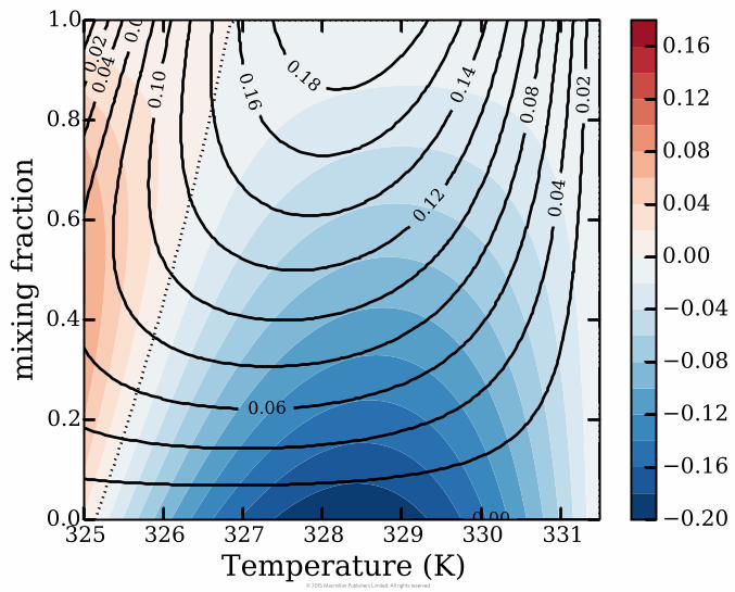
We have considered the mass loading of extra liquid water in the mixture. The temperature T2 below the 18
interface does not change, but varies from the warm adiabat (332 K) to the cold adiabat (325 K). We 19
display the value of and in Fig. S1. 20
Moist convection in hydrogen atmospheres and the frequency of Saturn’s giant storms
Cheng Li and Andrew P. Ingersoll
© 2015 Macmillan Publishers Limited. All rights reserved

At the start of the radiative cooling phase, we find that the mixture is always less dense than the fluid 21
below the interface and more dense than the fluid above it, meaning that the interface is stable. However 22
near the end of the cooling phase the mixture is less dense than the fluid above, and the interface is 23
unstable. Depending on the value of f, which is unknown, this could hasten the onset of convection and 24
decrease the time between giant storms by up to 25%. Given the other uncertainties, such as the water 25
vapor mixing ratio at depth, the 25% decrease has no significant effect on the model results. 26
27
S2. More details about the numerical model 28
The axisymmetric primitive equations in log-pressure coordinates are: 29
(S2.1)
(S2.2)
∑
(S2.3)
(S2.4)
(S2.5)
∑
∑
(S2.6)
(
)
(
)
(S2.7)
(S2.8)
(
)
(
)
(S2.9)
© 2015 Macmillan Publishers Limited. All rights reserved

where are radial, azimuthal and vertical winds. are potential temperature, temperature and 30
virtual temperature. is the mass streamfunction; . are microphysical 31
variables. They represent the latent heat, molecular mass ratio to dry air, mole mixing ratio, saturation 32
mixing ratio and condensation rate for condensable species i (i = NH3, H2O) respectively. are the 33
gas constant and specific heat capacity for dry air. are the temperature and density scale 34
height at bar. are the radial distance and log-pressure coordinate:
. are the 35
geopotential height and gravity. Eddy viscosity are included in the momentum equations to 36
damp out the energy. Since their values are unknown, we choose a small enough value ( 37
to both maintain numerical stability and damp out the energy. Any value larger 38
than the current one will result in a decrease of the azimuthal wind and the cooling time. Boundary 39
conditions are applied such that pressure gradient vanishes ( at the lower boundary and the vertical 40
velocity vanishes ( ) at the upper boundary due to the strong stratification of the stratosphere2. We 41
have moved the lower (upper) boundary low (high) enough to minimize the effects of boundary 42
conditions. Currently, the lower boundary is 30 bars and the upper boundary is 10 mbar. The positions of 43
lower and upper boundary have negligible effects on the result when the lower boundary is placed deeper 44
than 25 bars and the upper boundary higher than 50 mbar. The largest radial distance in the model is 45
m and two energy absorbing layers are placed at the top and right part of the domain. 46
47
S3. Sensitivity tests for the choices of 48
Fig. S2 has 9 panels showing the equilibrated temperature and azimuthal wind for a combination 49
with being 1.0%, 1.1%, 1.2% and being 100 km, 200 km, 300 km. Here η is the deep water vapor 50
mixing ratio and r0 is the Gaussian radius of the initial disturbance. Larger water mixing ratio results in 51
large temperature difference between the warm and cold adiabat, thereby larger wind speed and 52
tropospheric warming. Different values of do not change the overall structure of the wind and the 53
© 2015 Macmillan Publishers Limited. All rights reserved

warming because those variables are largely related to the deformation radius of the atmosphere and are 54
insensitive to the initial conditions such as . 55
56
S4. Numerical method of calculating the top cooling scheme 57
In the section of radiative cooling phase in the manuscript, we presented our scheme for calculating the 58
multi-decadal cooling phase, where the troposphere loses heat from the top. An interface develops 59
between the convecting layers above and the undisturbed layers below. We described the interface 60
moving down through our numerical grid as a two-step process. Step 1 (entrainment step) occurs when 61
the interface is neutrally stable and moves down a level, entraining all the fluid in the grid box below. 62
Step 2 (cooling step) occurs over a period of time and involves lowering the temperature of the fluid 63
above until the interface is neutral again. Here we describe this process in greater detail. 64
65
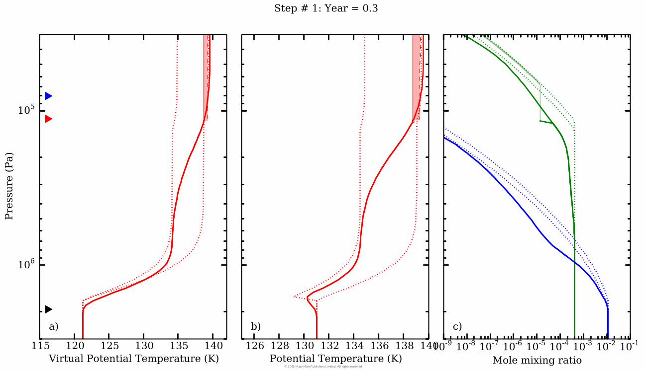
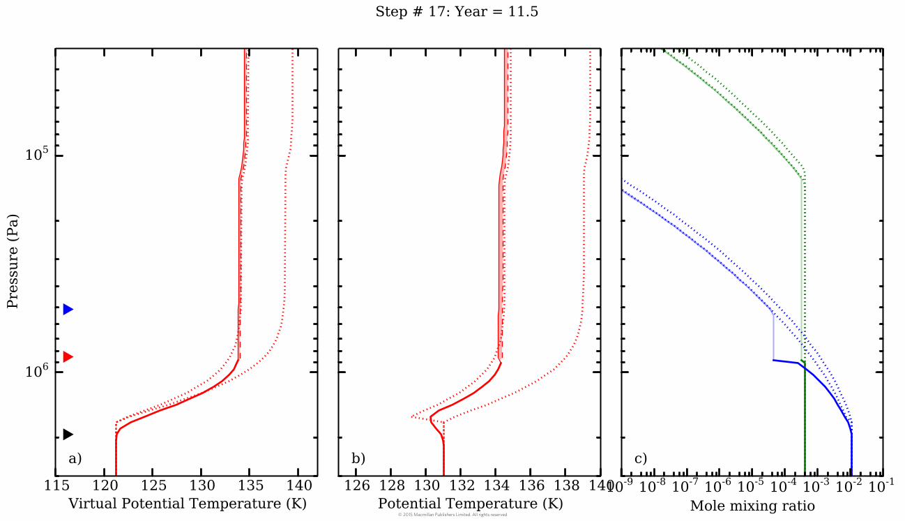
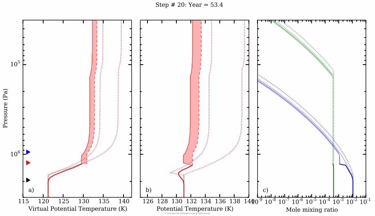
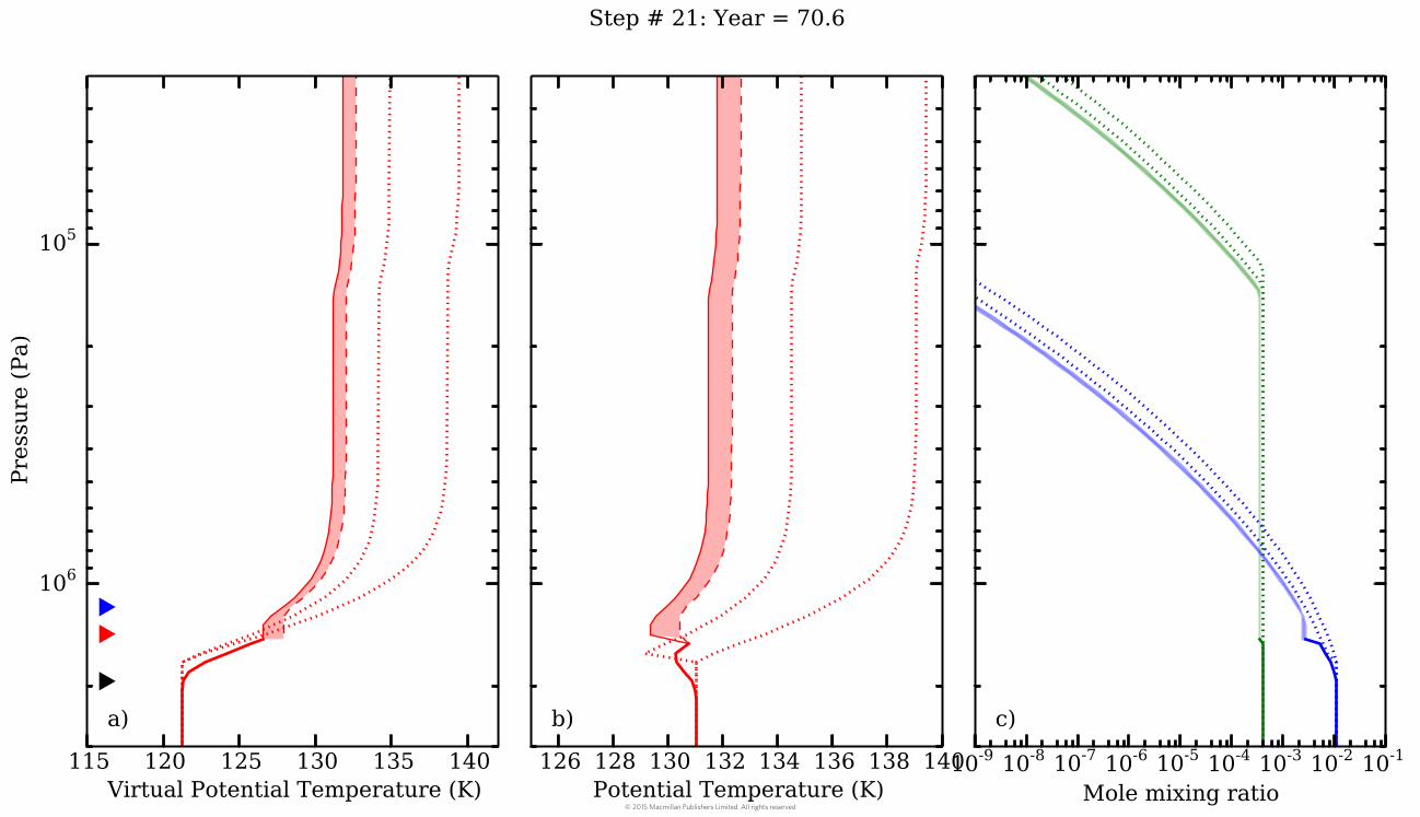
The numerical results calculated by the above scheme at every other grid box are displayed as a time 66
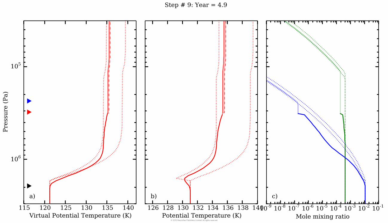
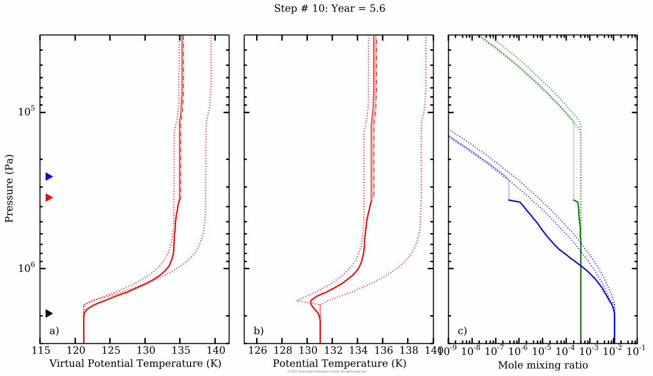
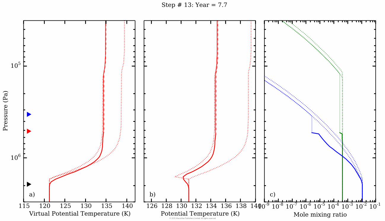
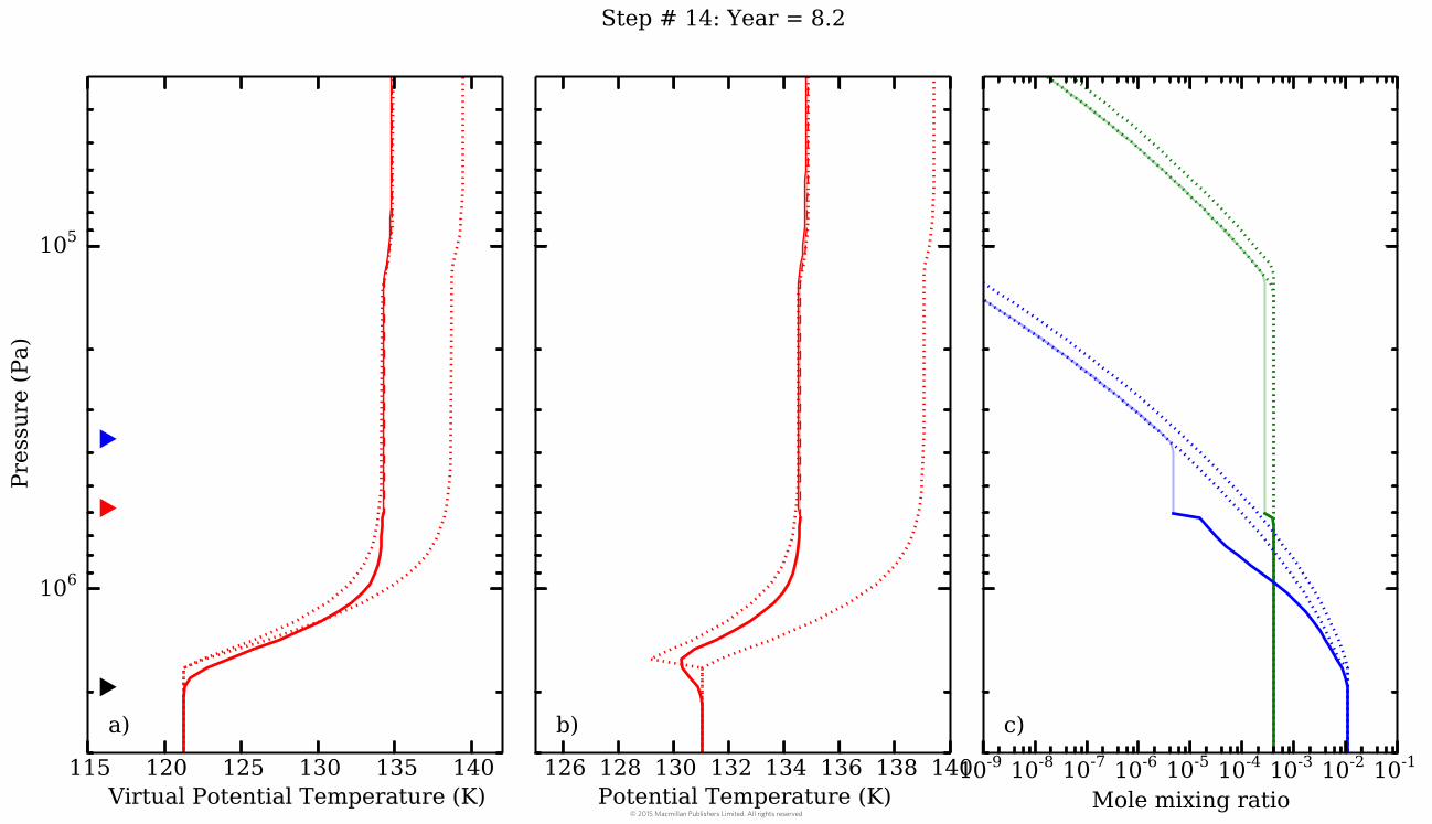
series in Fig. S3. At each time, the left panel (a) shows virtual potential temperature, whose vertical 67
gradient determines whether the column is stable or unstable to convection. The middle panel (b) shows 68
potential temperature, which gives the contribution of temperature alone to the stability of the column. 69
The right panel (c) gives the mixing ratios of water (blue) and ammonia (green). Temperature itself, 70
which falls off monotonically with altitude at all times, is not shown. The primordial profile, following 71
geostrophic adjustment after the last giant storm, is shown as a heavy solid line in the figure for Year = 72
0.3. This profile becomes a remnant as the interface moves downward and the primordial layer shrinks. 73
The warm and cold moist adiabats—the solid and dashed red lines in Fig. 2 of the main paper—are shown 74
as dotted lines in Fig. S3. There are three characteristic features of the potential temperature profile in 75
panel (b). Above the 1 bar level, the profile is close to the warm adiabat. Between 1 bar and 6 bars, the 76
profile follows a transition from the warm adiabat to the cold adiabat. In pressure levels deeper than 6 77
© 2015 Macmillan Publishers Limited. All rights reserved
bars, potential temperature decreases with depth and contributes to the stability of the column, but then it 78
overshoots and creates a potential temperature minimum at the cloud base. However, this negative 79
potential temperature lapse rate is stable because it is compensated by the increase of the mean molecular 80
weight to deep pressure levels. Therefore, the lapse rate of virtual potential temperature in panel (a) is still 81
positive, and the profile is stable. 82
83
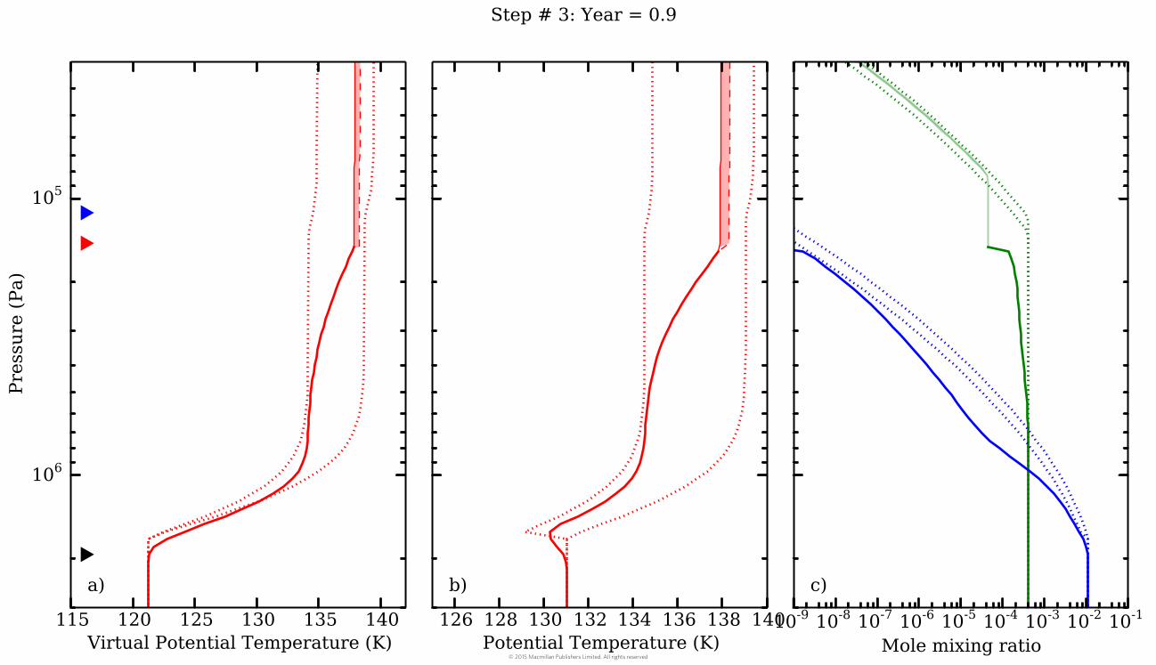
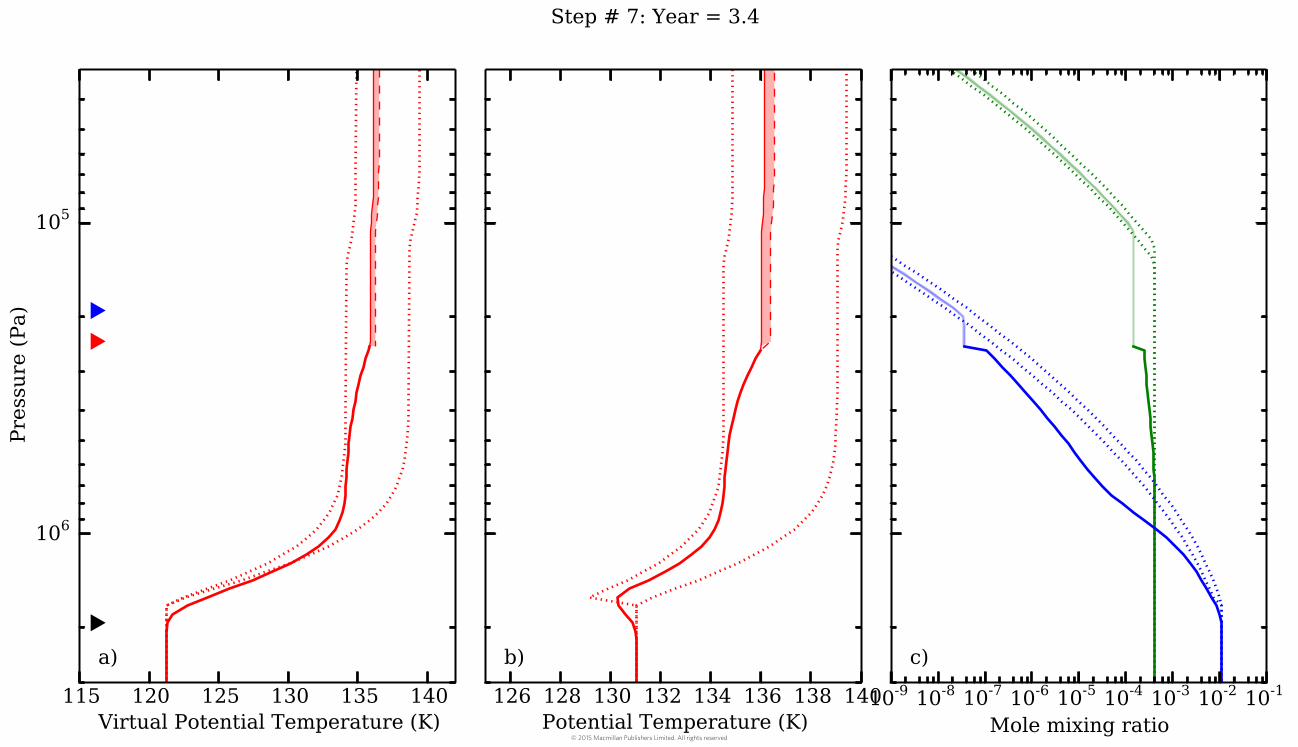
The lower boundaries of layers 1, 2, and 3 described in the main text are shown as blue, red, and black 84
triangles, respectively. To visualize the process, it is helpful to click through the entire time series from 85
Year = 0.3 to Year = 74.0. The four layer structure described in the section of radiative cooling phase in 86
the manuscript is best represented at Year = 2.0. Layer 1 is directly subject to radiative cooling at the top. 87
It experience condensation of ammonia and water. Its temperature profile is moist adiabat and the mixing 88
ratio of the constituent is either the saturated value or a constant. Layer 1 is supported by the dry 89
convecting layer 2 below it. Layer 2 has two roles. First, because it is unsaturated, any precipitation in 90
layer 1 will re-evaporate in layer 2. Layer 2 serves as reservoir that holds the extra moisture in layer 1. 91
Column integrated moisture in layers 1 and 2 is conserved. Second, the lower boundary of layer 2 (the 92
interface) separates the convective layers (layers 1 and 2) from the non-convective layers (layer 3) by a 93
jump in temperature and mixing ratios. In the numerical model, the jump is a discontinuity, but in the 94
figure it appears as a steep gradient. Below Layer 2 is layer 3 where the atmosphere is stably stratified and 95
does not convect to mix the minor constituents. Since layer 3 is not disturbed by convection, its 96
temperature and mixing ratio profiles are set by the previous geostrophic adjustment. Layer 3 transits into 97
layer 4 at about 20 bars. Layer 4 is the deep interior, which is a dry adiabat with the minor constituents 98
well mixed. It is somewhat arbitrary to define the precise level of the boundary between layer 3 and layer 99
4 because the temperature and mixing ratios are continuously changing. 100
101
© 2015 Macmillan Publishers Limited. All rights reserved

As stated in the main manuscript, the vertical potential temperature profile (shaded region in Fig. S3 after 102
year 9) evolves to lower values than the cold adiabat (left dotted line in Fig. S3a) around year 9, as shown 103
in Fig. S3. However the interface (red triangle) remains stable relative to the cold adiabat. This is because 104
the troposphere is cooling from the top down, with an initial profile that is unsaturated and stable (thick 105
solid line in step #1 of Fig. S3). After year 9, the profile is to the left of the cold adiabat in the upper 106
troposphere, but it crosses to the right in the dry adiabatic layer (between the blue and red triangles), 107
making the interface stable. 108
109
Here we present the actual numerical implementation of the above scheme. Suppose the atmospheric 110
column is divided into n discrete cells centered at pressure, , from top to bottom. The 111
profile of temperature and mixing ratios are
where w represents “water” and a represents 112
“ammonia”. These variables are cell averaged quantities from over the width of the 113
remaining anticyclone after the geostrophic adjustment (section 3). The boundary values between cells are 114
calculated by linear interpolation. We define and as the molecular weights of water and ammonia 115
relative to that of the H2-He mixture. Then the corresponding mass mixing ratios are: 116
(S4.1)
Mass per unit area of each cell is: 117
(S4.2)
Column integrated moisture per unit area above the cell k is: 118
∑
∑
(S4.3)
Column integrated enthalpy per unit area above the cell k is: 119
© 2015 Macmillan Publishers Limited. All rights reserved

∑
(S4.4)
If the bottom of layer 2 is located at the bottom of cell k: , then all quantities above that level 120
are determined by
, at pressure . This is because layer 2 is dry adiabatic with constant 121
mixing ratios and layer 1 is moist adiabatic with saturation mixing ratios. One simply follows the dry 122
adiabat up to cloud base—the lifting condensation level for each gas—and then follows the moist adiabat 123
from that point on. This gives
, so one can calculate ,
. 124
125
Let the initial profile of temperature and mixing ratios to be
. We proceed 126
from one entrainment step to the next, during which time the interface moves down from pressure 127
to pressure . We assume the preceding entrainment step ended with a stable interface at pressure 128
, as indicated by the dashed line in Fig. S3. In other words, the virtual temperature above the 129
interface was greater than that below the interface: 130
(S4.5)
The cycle begins with the slow cooling step, which reduces and , with
adjusted to 131
maintain the dry/moist adiabat and conserved the total moisture per unit area: 132
(S4.6)
where
are the initial column-integrated moisture per unit area. When equation (S4.5) becomes 133
an equality, as indicated by the thin solid line in Fig. S3, the cooling step ends and the next entrainment 134
step begins. The proper temperature and moistures at cell k:
, when the cooling step ends, are 135
solved using Newton’s iteration method to satisfy equations (S4.5) and (S4.6). After we solved for these 136
quantities, we can go for the vertical profiles of
by following a dry adiabat and 137
then moist adiabat. The column-integrated enthalpy per unit area is bookkept as using equation (S4.4). 138
© 2015 Macmillan Publishers Limited. All rights reserved
139
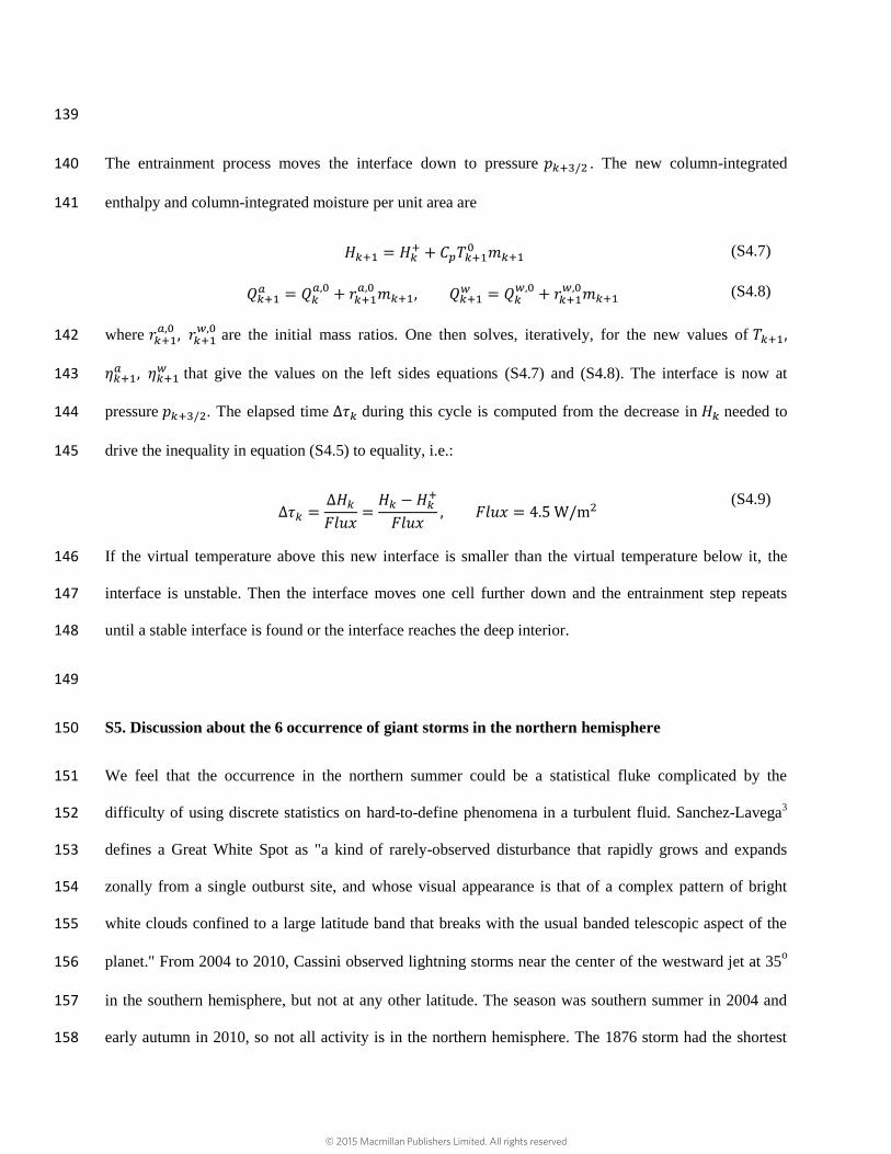
The entrainment process moves the interface down to pressure . The new column-integrated 140
enthalpy and column-integrated moisture per unit area are 141
(S4.7)
(S4.8)
where
are the initial mass ratios. One then solves, iteratively, for the new values of 142
that give the values on the left sides equations (S4.7) and (S4.8). The interface is now at 143
pressure . The elapsed time during this cycle is computed from the decrease in needed to 144
drive the inequality in equation (S4.5) to equality, i.e.: 145
(S4.9)
If the virtual temperature above this new interface is smaller than the virtual temperature below it, the 146
interface is unstable. Then the interface moves one cell further down and the entrainment step repeats 147
until a stable interface is found or the interface reaches the deep interior. 148
149
S5. Discussion about the 6 occurrence of giant storms in the northern hemisphere 150
We feel that the occurrence in the northern summer could be a statistical fluke complicated by the 151
difficulty of using discrete statistics on hard-to-define phenomena in a turbulent fluid. Sanchez-Lavega3 152
defines a Great White Spot as "a kind of rarely-observed disturbance that rapidly grows and expands 153
zonally from a single outburst site, and whose visual appearance is that of a complex pattern of bright 154
white clouds confined to a large latitude band that breaks with the usual banded telescopic aspect of the 155
planet." From 2004 to 2010, Cassini observed lightning storms near the center of the westward jet at 35o 156
in the southern hemisphere, but not at any other latitude. The season was southern summer in 2004 and 157
early autumn in 2010, so not all activity is in the northern hemisphere. The 1876 storm had the shortest 158
© 2015 Macmillan Publishers Limited. All rights reserved
lifetime of 26 days, and until the 2010-2011 storm, the 1903 storm had the longest lifetime of 150 days. 159
The lifetime of the 2010-2011 storm was ~200 days. The fact that we are dealing with real phenomena in 160
a turbulent fluid adds uncertainty to statistical inferences. Even if we were dealing with six coin flips, the 161
probability of their all coming out the same is 1/32. Since one of the great storms was at a latitude of 2 ± 162
3°N, the number of coins should probably be reduced to five, for which the probability of their all falling 163
in one hemisphere is 1/16. What seems more likely to us is a preference for the sunlit hemisphere, with a 164
statistical fluke favoring the north. A preference for the sunlit hemisphere and for the extrema of the zonal 165
jets might have a physical basis, but we leave that for another paper. 166
167
S6. Discussion about radiative heat transfer near the cloud base 168
Guillot4 points out that the giant planets might not be fully convective—that at some levels the radiative 169
opacity is small enough that the internal heat flux could be carried by radiation. For Saturn, they show 170
that a radiative zone could develop in the layer from 300 K < T < 450 K, which spans cloud base 171
according to our Fig. 2. Then the cooling shown in Figs. 5 and S3 might not occur, and the atmosphere 172
above cloud base might reach a steady state, with 4.5 W m-2
coming in at the bottom and 4.5 W m-2
going 173
out at the top. The interface at cloud base, stabilized by the molecular weight gradient, would never cool 174
enough to initiate a giant storm. In this situation, one should remember that atmospheric temperature 175
profile has CAPE, which means it has the potential to convect when the stable interface is broken by other 176
mechanism such as the re-evaporation of condensates from above5. 177
178
However, the existence of a radiative zone is uncertain. It vanishes if water clouds are present around this 179
level, as shown in Fig. 6 of Guillot. If it vanishes, then giant storms can occur. If radiation delivers more 180
than zero but less than the 4.5 W m-2
needed to maintain steady state, then the layers above will still cool 181
but at a slower rate. This lengthens the interval between giant storms, but it does not prevent them. 182
© 2015 Macmillan Publishers Limited. All rights reserved
Despite the uncertainty, we shall assume that the time between giant storms is set by the time it takes the 183
atmosphere to cool from the warm adiabat to the cold one, as illustrated in Fig. 2. 184
185
186
Reference 187
1 Emanuel, K. A. Atmospheric convection. (Oxford University Press, 1994). 188
2 Achterberg, R. K. & Ingersoll, A. P. A Normal-Mode Approach to Jovian Atmospheric Dynamics. 189
J Atmos Sci 46, 2448-2462 (1989). 190
3 Sanchez-Lavega, A. Saturn's Great White Spots. Chaos 4, 341-353 (1994). 191
4 Guillot, T., Gautier, D., Chabrier, G. & Mosser, B. Are the Giant Planets Fully Convective. Icar 192
112, 337-353 (1994). 193
5 Sugiyama, K., Nakajima, K., Odaka, M., Kuramoto, K. & Hayashi, Y. Y. Numerical simulations 194
of Jupiter's moist convection layer: Structure and dynamics in statistically steady states (vol 229, 195
pg 71, 2014). Icar 231, 407-408 (2014). 196
197
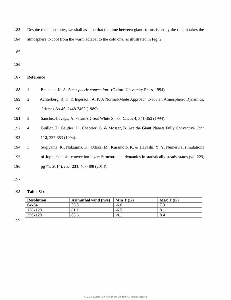
Table S1: 198
Resolution Azimuthal wind (m/s) Min T (K) Max T (K)
64x64 56.8 -6.6 7.3
128x128 81.1 -6.5 8.1
256x128 83.6 -8.1 8.4
199
© 2015 Macmillan Publishers Limited. All rights reserved

Figure legends 200
Figure S1: Mixing diagram across the temperature discontinuity at the cloud base. X-axis is the 201
temperature above the cloud base ( ) and y-axis is the fraction of the parcel coming from the top ( ). 202
The lower and upper limit of the temperature axis is chosen to be the temperature of the cold and the 203
warm adiabat at the cloud base. The solid curves show , which is always positive. The colored 204
contours show , which is positive (red) to the left and negative (blue) to the right. The mixture 205
is stable (unstable) with respect to the atmosphere above cloud base in the blue (red) zones, respectively. 206
207
Figure S2: Residual azimuthal wind (dashed contours) and temperature anomaly (colored contours) 208
for different combinations of parameters. The parameters are indicated at the bottom of each panel. 209
210
Figure S3: A series of cooling steps. Panel (a) and Panel (c) represent the same quantity in Fig. 5. Panel 211
(b) is the potential temperature defines as (
)
. bar, is the reference temperature. Two 212
dotted lines represent the cold and warm moist adiabat as those in Fig. 2. The thick solid red line is the 213
potential temperature profile after the geostrophic adjustment. The shaded region shows one cooling step, 214
from right to left. The right boundary (dashed line) shows the profile after the preceding entrainment step. 215
The left boundary (solid line) shows the profile just before the next entrainment step. Only stable 216
interfaces are shown in this figure. 217
218
Table legend 219
Table 1: Resolution dependency test. Tabulated values are maximum azimuthal wind, minimum 220
temperature anomaly and maximum temperature anomaly for 3 different resolutions. The first number in 221
the resolution is the horizontal points and the second number is the vertical points. 222
© 2015 Macmillan Publishers Limited. All rights reserved
325 326 327 328 329 330 331
Temperature (K)
0.0
0.2
0.4
0.6
0.8
1.0m
ixin
g f
ract
ion
0.00
0.0
2
0.0
2
0.0
4
0.0
4
0.06
0.0
6
0.0
8
0.1
0
0.12
0.1
40.1
6
0.18
0.20
0.16
0.12
0.08
0.04
0.00
0.04
0.08
0.12
0.16
© 2015 Macmillan Publishers Limited. All rights reserved

102
103
104
Pre
ssu
re (
mb
ar)
η = 1.0% r0 = 1.0 km
-24
-20
-16 -1
2
-8 -4
0
0
η = 1.0% r0 = 2.0 km
-30-25
-20
-15
-10
-5 0
0η = 1.0% r0 = 3.0 km
-30
-24-18
-12
-6 0
0
102
103
104
Pre
ssu
re (
mb
ar)
η = 1.1% r0 = 1.0 km
-70
-60-50-40-30
-20
-10
0
0
η = 1.1% r0 = 2.0 km
-75-60
-45
-30
-15
0
0
η = 1.1% r0 = 3.0 km
-75-60
-45
-30
-15
0
2 4 6 8Distance (103 km)
102
103
104
Pre
ssu
re (
mb
ar)
η = 1.2% r0 = 1.0 km
-75
-60
-45
-30
-15
0
2 4 6 8Distance (103 km)
η = 1.2% r0 = 2.0 km
-120-100
-80
-60-40
-20
0
0
0
2 4 6 8Distance (103 km)
η = 1.2% r0 = 3.0 km
-100
-80-60
-40
-20
0
8
6
4
2
0
2
4
6
8
© 2015 Macmillan Publishers Limited. All rights reserved
115 120 125 130 135 140Virtual Potential Temperature (K)
105
106
Pre
ssu
re (
Pa)
a)
126 128 130 132 134 136 138 140Potential Temperature (K)
b)
10-9 10-8 10-7 10-6 10-5 10-4 10-3 10-2 10-1
Mole mixing ratio
c)
Step # 1: Year = 0.3
© 2015 Macmillan Publishers Limited. All rights reserved

115 120 125 130 135 140Virtual Potential Temperature (K)
105
106
Pre
ssu
re (
Pa)
a)
126 128 130 132 134 136 138 140Potential Temperature (K)
b)
10-9 10-8 10-7 10-6 10-5 10-4 10-3 10-2 10-1
Mole mixing ratio
c)
Step # 2: Year = 0.6
© 2015 Macmillan Publishers Limited. All rights reserved
115 120 125 130 135 140Virtual Potential Temperature (K)
105
106
Pre
ssu
re (
Pa)
a)
126 128 130 132 134 136 138 140Potential Temperature (K)
b)
10-9 10-8 10-7 10-6 10-5 10-4 10-3 10-2 10-1
Mole mixing ratio
c)
Step # 3: Year = 0.9
© 2015 Macmillan Publishers Limited. All rights reserved

115 120 125 130 135 140Virtual Potential Temperature (K)
105
106
Pre
ssu
re (
Pa)
a)
126 128 130 132 134 136 138 140Potential Temperature (K)
b)
10-9 10-8 10-7 10-6 10-5 10-4 10-3 10-2 10-1
Mole mixing ratio
c)
Step # 4: Year = 1.4
© 2015 Macmillan Publishers Limited. All rights reserved

115 120 125 130 135 140Virtual Potential Temperature (K)
105
106
Pre
ssu
re (
Pa)
a)
126 128 130 132 134 136 138 140Potential Temperature (K)
b)
10-9 10-8 10-7 10-6 10-5 10-4 10-3 10-2 10-1
Mole mixing ratio
c)
Step # 5: Year = 2.0
© 2015 Macmillan Publishers Limited. All rights reserved

115 120 125 130 135 140Virtual Potential Temperature (K)
105
106
Pre
ssu
re (
Pa)
a)
126 128 130 132 134 136 138 140Potential Temperature (K)
b)
10-9 10-8 10-7 10-6 10-5 10-4 10-3 10-2 10-1
Mole mixing ratio
c)
Step # 6: Year = 2.7
© 2015 Macmillan Publishers Limited. All rights reserved
115 120 125 130 135 140Virtual Potential Temperature (K)
105
106
Pre
ssu
re (
Pa)
a)
126 128 130 132 134 136 138 140Potential Temperature (K)
b)
10-9 10-8 10-7 10-6 10-5 10-4 10-3 10-2 10-1
Mole mixing ratio
c)
Step # 7: Year = 3.4
© 2015 Macmillan Publishers Limited. All rights reserved

115 120 125 130 135 140Virtual Potential Temperature (K)
105
106
Pre
ssu
re (
Pa)
a)
126 128 130 132 134 136 138 140Potential Temperature (K)
b)
10-9 10-8 10-7 10-6 10-5 10-4 10-3 10-2 10-1
Mole mixing ratio
c)
Step # 8: Year = 4.1
© 2015 Macmillan Publishers Limited. All rights reserved
115 120 125 130 135 140Virtual Potential Temperature (K)
105
106
Pre
ssu
re (
Pa)
a)
126 128 130 132 134 136 138 140Potential Temperature (K)
b)
10-9 10-8 10-7 10-6 10-5 10-4 10-3 10-2 10-1
Mole mixing ratio
c)
Step # 9: Year = 4.9
© 2015 Macmillan Publishers Limited. All rights reserved
115 120 125 130 135 140Virtual Potential Temperature (K)
105
106
Pre
ssu
re (
Pa)
a)
126 128 130 132 134 136 138 140Potential Temperature (K)
b)
10-9 10-8 10-7 10-6 10-5 10-4 10-3 10-2 10-1
Mole mixing ratio
c)
Step # 10: Year = 5.6
© 2015 Macmillan Publishers Limited. All rights reserved

115 120 125 130 135 140Virtual Potential Temperature (K)
105
106
Pre
ssu
re (
Pa)
a)
126 128 130 132 134 136 138 140Potential Temperature (K)
b)
10-9 10-8 10-7 10-6 10-5 10-4 10-3 10-2 10-1
Mole mixing ratio
c)
Step # 11: Year = 6.3
© 2015 Macmillan Publishers Limited. All rights reserved

115 120 125 130 135 140Virtual Potential Temperature (K)
105
106
Pre
ssu
re (
Pa)
a)
126 128 130 132 134 136 138 140Potential Temperature (K)
b)
10-9 10-8 10-7 10-6 10-5 10-4 10-3 10-2 10-1
Mole mixing ratio
c)
Step # 12: Year = 7.0
© 2015 Macmillan Publishers Limited. All rights reserved
115 120 125 130 135 140Virtual Potential Temperature (K)
105
106
Pre
ssu
re (
Pa)
a)
126 128 130 132 134 136 138 140Potential Temperature (K)
b)
10-9 10-8 10-7 10-6 10-5 10-4 10-3 10-2 10-1
Mole mixing ratio
c)
Step # 13: Year = 7.7
© 2015 Macmillan Publishers Limited. All rights reserved
115 120 125 130 135 140Virtual Potential Temperature (K)
105
106
Pre
ssu
re (
Pa)
a)
126 128 130 132 134 136 138 140Potential Temperature (K)
b)
10-9 10-8 10-7 10-6 10-5 10-4 10-3 10-2 10-1
Mole mixing ratio
c)
Step # 14: Year = 8.2
© 2015 Macmillan Publishers Limited. All rights reserved

115 120 125 130 135 140Virtual Potential Temperature (K)
105
106
Pre
ssu
re (
Pa)
a)
126 128 130 132 134 136 138 140Potential Temperature (K)
b)
10-9 10-8 10-7 10-6 10-5 10-4 10-3 10-2 10-1
Mole mixing ratio
c)
Step # 15: Year = 8.6
© 2015 Macmillan Publishers Limited. All rights reserved

115 120 125 130 135 140Virtual Potential Temperature (K)
105
106
Pre
ssu
re (
Pa)
a)
126 128 130 132 134 136 138 140Potential Temperature (K)
b)
10-9 10-8 10-7 10-6 10-5 10-4 10-3 10-2 10-1
Mole mixing ratio
c)
Step # 16: Year = 9.4
© 2015 Macmillan Publishers Limited. All rights reserved
115 120 125 130 135 140Virtual Potential Temperature (K)
105
106
Pre
ssu
re (
Pa)
a)
126 128 130 132 134 136 138 140Potential Temperature (K)
b)
10-9 10-8 10-7 10-6 10-5 10-4 10-3 10-2 10-1
Mole mixing ratio
c)
Step # 17: Year = 11.5
© 2015 Macmillan Publishers Limited. All rights reserved

115 120 125 130 135 140Virtual Potential Temperature (K)
105
106
Pre
ssu
re (
Pa)
a)
126 128 130 132 134 136 138 140Potential Temperature (K)
b)
10-9 10-8 10-7 10-6 10-5 10-4 10-3 10-2 10-1
Mole mixing ratio
c)
Step # 18: Year = 18.1
© 2015 Macmillan Publishers Limited. All rights reserved

115 120 125 130 135 140Virtual Potential Temperature (K)
105
106
Pre
ssu
re (
Pa)
a)
126 128 130 132 134 136 138 140Potential Temperature (K)
b)
10-9 10-8 10-7 10-6 10-5 10-4 10-3 10-2 10-1
Mole mixing ratio
c)
Step # 19: Year = 32.8
© 2015 Macmillan Publishers Limited. All rights reserved
115 120 125 130 135 140Virtual Potential Temperature (K)
105
106
Pre
ssu
re (
Pa)
a)
126 128 130 132 134 136 138 140Potential Temperature (K)
b)
10-9 10-8 10-7 10-6 10-5 10-4 10-3 10-2 10-1
Mole mixing ratio
c)
Step # 20: Year = 53.4
© 2015 Macmillan Publishers Limited. All rights reserved
115 120 125 130 135 140Virtual Potential Temperature (K)
105
106
Pre
ssu
re (
Pa)
a)
126 128 130 132 134 136 138 140Potential Temperature (K)
b)
10-9 10-8 10-7 10-6 10-5 10-4 10-3 10-2 10-1
Mole mixing ratio
c)
Step # 21: Year = 70.6
© 2015 Macmillan Publishers Limited. All rights reserved

115 120 125 130 135 140Virtual Potential Temperature (K)
105
106
Pre
ssu
re (
Pa)
a)
126 128 130 132 134 136 138 140Potential Temperature (K)
b)
10-9 10-8 10-7 10-6 10-5 10-4 10-3 10-2 10-1
Mole mixing ratio
c)
Step # 22: Year = 74.0
© 2015 Macmillan Publishers Limited. All rights reserved