does wealth inequality help informal insurance?

DOES WEALTH INEQUALITY HELP INFORMAL INSURANCE?

GARANCE GENICOT

ABSTRACT. This paper investigates the effects of inequality in the presence ofvoluntary risk-sharing. In any period, an agent’s resources are composed of hisshare of a secure endowment (wealth, land) and a random component (laborincome). To be sure, the distribution of wealth does not affect the Pareto op-timal payoff vectors but, by changing the autarchic utilities, affects the set ofthese payoff vectors that are self-enforcing. When risk-sharing is not perfect, atransfer of wealth from an agent to the other is shown to cause the frontier ofthe self-enforcing payoff vectors to pivot. The more power an agent has, thelarger the change in his utility from an increase in his share of wealth.

Surprisingly, inequality is shown to help risk-sharing in a large range ofcases. Regressive transfers of wealth increase the likelihood of perfect insuranceall utility functions displaying hyperbolic absolute risk aversion (HARA) at theexception of the constant absolute risk aversion for which, as it is well known,wealth effects are absent. Moreover, introducing wealth inequality between theagents can increase the sum of utilities of the agent, thereby being desirable fora social planner maximizing a symmetric and additive welfare function.

These results have important welfare and policy implications for redistribu-tion programs such as land reform.

We also show that when risk aversion is decreasing individuals tend to prefersharing risk with poorer partners.

JEL Classification Numbers: D31, D8, D63, O17, Q15.

Key Words: Inequality, Risk-Sharing, Informal Insurance, Redistribution, LandReform.

Date: November 2006.VERY PRELIMINARY DRAFT. Comments welcome. Please address correspondence to

[email protected]

2

1. INTRODUCTION

In most of the developing world, people are exposed to substantial, even cat-astrophic, risk and mitigating risk is a central concern. A high degree of depen-dence on agricultural production, widespread poverty and the lack of access toformal insurance and credit, make the need for consumption smoothing partic-ularly acute. As a result, most households in low-income countries deal withadverse economic events through informal insurance, arrangements arising be-tween individuals and communities on a personalized basis (Morduch 1999).Individuals typically respond to the large fluctuations in their income by engag-ing in informal risk-sharing: providing each other with help, gifts and transferswith some expected reciprocity.

There is considerable evidence of the presence of some but limited insurancein village communities (Deaton 1992, Townsend 1994, Udry 1994, Attanasioand Davis 1996, Jalan and Ravallion 1999, Grimard 1997, Gertler and Gruber2002, Ligon, Thomas and Worrall 2000, Foster and Rosenzweig 2002). Theselimitations could result from various incentive constraints. Asymmetry of infor-mation, moral hazard and lack of enforceability are all potential impediments torisk sharing. The most important constraint appears to arise from the lack of en-forceability of risk-sharing agreements.1 Explicit, legally binding, and crediblyenforceable contracts not being available, these agreements must be designed toelicit voluntary participation. This constraint often seriously limits the extent ofinsurance informal risk-sharing agreements can provide.

There is a growing theoretical literature on self-enforcing risk-sharing agree-ments. Some important contributions are Posner (1981), Kimball (1988), Coateand Ravallion (1993), Kocherlakota (1996), Kletzer and Wright (2000), Ligon etal. (2000), and Genicot and Ray (2003). However, most studies focus on risk-sharing among identical agents. Two exceptions are Krueger and Perri (2002)and Sadoulet (2001) who consider different sources of heterogeneity than us.We will discuss the parallels in more details in Sections 4 and 5.

In this paper, we study risk-sharing between individuals facing the same riskbut differing in their mean income, and investigate the impact of this inequalityon the agreement they engage in. Consider two agents whose resources, at anydate, are composed of their share of a secure endowment, that we shall calltheir permanent income or wealth, and a random component. If it were not fortheir wealth, the two agents would be identical. Changes in the distribution

1Udry (1994), for instance, finds this constraint to be the most important in describing thestructure of reciprocal agreements in rural northern Nigeria.

DOES WEALTH INEQUALITY HELP INFORMAL INSURANCE? 3

of wealth do not affect the aggregate resources at any time, and therefore thePareto set is unchanged. However, by changing their autarchic utilities, thewealth distribution affects the set of self-enforcing payoff vectors.

Redistribution of wealth from an agent to the other is shown to cause a pivotof the frontier of the self-enforcing payoff vectors. The more power an agenthas, the larger the change in his utility from an increase in his share of wealth.

Inequality is actually shown to help risk-sharing in a large range of cases. Re-gressive transfers of wealth increase the likelihood of perfect insurance for allutility functions displaying hyperbolic absolute risk aversion (HARA) — whichencompasses all the utility functions typically used — at the exception of theconstant absolute risk aversion for which, as it is well known, wealth effects areabsent. Moreover, introducing wealth inequality between the agents often in-crease the transfers made in the constrained optimal agreement. Hence, thoughthe net welfare effect is in general ambiguous, regressive transfers have the po-tential to increase the sum of the agent utilities.

These results are interesting in several dimensions. First, they highlight apotential cost of redistribution in the form of a reduction in risk-sharing or in-formal insurance. The implications of such finding are clearly important for thedesign of redistribution policies such as land reform.

There is a large literature identifying potential costs or benefits of inequal-ity. Various reasons have been advanced showing that inequality can be ben-eficial such as convex savings (Bourguignon 1981), changes in the balance ofpower in the political system (Bertola 1993, Alesina and Rodrik 1994, Perssonand Tabellini 1994), credit constraints and investment thresholds (Banerjee andNewman 1993, Galor and Zeira 1993, Murgai, Winters, Sadoulet and de Janvry2002, Aghion and Bolton 1997). However, as far we know, the effect of inequal-ity on informal insurance and its welfare consequences has not been studiedbefore.

Second, the paper shows that income levels are an important determinant ofchoice of partner in risk-sharing agreements. We show that, when risk aversionis decreasing, individuals tend to prefer sharing risk with poorer agents. This isbecause the latter are willing to transfer more in exchange for transfers in timeof need. However this does not necessarily imply that, if agents could formpairs to share risk, we would see assortative matching. In fact, checking for thestability of match is a complex object.

The rest of the paper is organized as follows. The next Section lays out thebasic model and describes the optimal allocation. Section 3 then presents the

4 GARANCE GENICOT

main results regarding the impact of inequality on risk-sharing. These resultsare illustrated by some numerical examples. In Section 4, we briefly discuss thequestion of choice of a risk sharing partner. Section 5 discusses some importantimplications of the paper and its limitations. Section 6 concludes. All proofs arerelegated to Section 7.

2. INFORMAL RISK-SHARING

Before stating and answering the questions of interest, we need to lay out thebasic setup of the risk-sharing problem without commitment.

2.1. Premises of the Model. Two agents, indexed by i ∈ {1, 2}, are engaged inthe production and consumption of a perishable good at any date t. Each agenti’s income at the beginning of each period yi is random. It is composed of asecure endowment wi, what we shall call their permanent income or wealth, anda random element εi so that

yi = wi + εi.

We think of these two components as two different sources of revenue: awealth component, for instance the ownership of trees would produce a regularendowment; and a labor income that fluctuates. Alternatively, in each period,the agents could experience a loss or fall sick, and this risk is additive.

The two agents are identical in all relevant dimensions but their wealth. Let zbe agent 1’s share of the aggregate wealth w such that

wi = ziw, z1 = z and z2 = 1− z, z ∈ [0, 1].

Without loss of generality, we normalize w at 1.

The distribution of the random components in the agent incomes (ε1t , ε

2t ) is

symmetric and independent over time. εit can take on a finite number of values

ε1 < ε2... < εN . Let S be the set of possible realizations for (ε1, ε2) and ps bethe probability of a particular state of the world s ∈ S (ps ≥ 0 and

∑s∈S

ps = 1).

Assume that there the state of the world (ε1, εN) has a positive probability. Foreach state s, denote by y(s) = (y1(s), y2(s)) the vector of realized incomes and byys =

∑i yi(s) the aggregate resources.

Our two agents have the same one-period von Neumann-Morgenstern utilityfunction u defined on consumption. Their lifetime expected utility from any


date t onwards is given by

E∞∑

j=0

δju(cit+j) ∀i ∈ {1, 2}.

where u is increasing, smooth and strictly concave, and δ ∈ (0, 1). is the discountrate.

2.2. Consumption Allocations. There is no storing technology available but in-dividuals can make transfers to each other in order to smooth their consump-tion. In the main part of the paper, we consider stationary transfers schemes(where transfers do depend only on the state of nature) but in a later section, wepoint out the results that can be extended to the case in which individuals makenon-stationary (history-dependent) transfers.

A consumption allocation c ≡ {c1(s), c2(s)}s∈S gives, for each state of natures, a nonnegative vector of consumptions c(s) that is feasible

∑i∈{1,2} c1(s) =∑

i∈{1,2} y1(s).

An allocation generates a vector of expected payoffs v = (v1, v2) (these are dis-counted expected payoffs for each individual). Let V be the upper boundaryof the collection of all feasible payoff vectors. It is the set of all Pareto optimalallocations. Each point on the frontier corresponds to the preferred allocationof a planner maximizing a weighted sum of the lifetime expected utilities of theindividuals for some welfare weights α = (α, 1− α) where α ∈ [0, 1].

2.3. Voluntary Risk-Sharing. To be sure, most of, if not all, the Pareto opti-mal allocations in V are generally not voluntary implementable. To be voluntaryimplementable, at each date, not only both individuals must ex-ante prefer theallocation to autarchy, before nature picks a state of the world, but they mustalso prefer it ex-post, once they know their realized income for the period.

In autarchy, each agent simply consumes his income at each date and enjoysa (discounted) lifetime expected utility of

(1) ua(zi) =1

1− δ

∑s∈S

p(s)u(yi(s)).

where yi(s) = zi + εi(s).

Hence, an allocation c is voluntary implementable given a division of wealth zif the following two conditions are satisfied:

6 GARANCE GENICOT

[PARTICIPATION.] For all i

(2)∑

s

psu(ci(s)) ≥ ua(zi)

[INCENTIVE.] For all i and every state of nature s,

(3) (1− δ)u(ci(s)) + δ∑

s′ps′u(ci(s

′)) ≥ (1− δ)u(yi(s)) + δua(zi)

To be sure, the set of feasible risk-sharing agreements and therefore the setof Pareto optimal allocations are independent of z since the aggregate income isunaffected by z. However, the division of wealth affects the autarchic utility andthereby does affect the set of implementable allocations.

2.4. Constrained Optimal Allocations. Given a level of utility v2 promised to 2,the following incentive-constrained optimization problem describes the utilitythat 1 can reach:

[THE z-PROBLEM.]

(4) maxc

v(v2, z) ≡∑

s

psu(c1(s))

subject to the incentive and participation constraints:∑

s

psu(ys − c1(s)) ≥ v2;(5)

(1− δ)u(c1(s)) + δ∑

s′ps′u(c1(s

′)) ≥ (1− δ)u(y1(s)) + δua1(z);(6)

(1− δ)u(ys − c1(s)) + δ∑

s′ps′u(ys′ − c1(s

′)) ≥ (1− δ)u(y2(s)) + δua2(z).(7)

with uai (z) =

∑s psu(yi(s)), yi(s) = zi+εs, ys =

∑i yi(s). Notice that the incentive

constraints imply that the participation constraints are satisfied.

It is easy to check that the objective function is strictly concave in c and the setof constraints convex. Hence, for any v2 for which a solution exists, this problemhas a unique solution that we shall denote c∗(v2, z). Let V ∗(z) be the set of theconstrained optimal payoffs vectors given z. These are generated by solvingthe z-problem for all possible values of v2. Abusing slightly notation we shalldenote by z, in these expressions, the distribution of wealth corresponding toz1 = z and z2 = 1− z.


For a given z and v2, the constrained optimal allocation c∗ is characterized bythe first-order conditions

(8)u′(c1(s))

u′(ys − c1(s))=

χ + µ2s

ps(1− δ) + δ

∑s′ µ

2s′

1 + µ1s

ps(1− δ) + δ

∑s′ µ

1s′

where µ1s and µ2

s are the multiplier on the incentive constraints (6) and (7) whenrealized state is s, and χ is the multiplier on the promise keeping constraint.This condition characterizes the way the ratio of marginal utility of the agents— their relative needs — responds to income shocks.

Denote as θ(s) the equilibrium ratio of marginal utilities (RMU) of the agentsin state s

θ(s) =u′(c∗1(s))u′(c∗2(s))

whose law of motion is given by equation (8).

If no incentive constraint binds in a state s, then the ratio of marginal utilitiesθ(s) of the agents is kept constant at

M =χ + δ

∑s′ µ

2s′

1 + δ∑

s′ µ1s′

.

If no incentive constraint ever binds then the ratio of marginal utilities of theagents is kept constant across all state of nature. This is perfect insurance. Theparticular level of RMU is given by the agents’ relative welfare weights. Whensome constraints do bind in other states then the importance of the welfareweights in determining the RMU in state s decreases. In in state s one of theagents’ incentive constraint binds, equation (8) tells us that the ration of mar-ginal utilities of the agents θ(s) is adjusted so as to increase that agent’s con-sumption level.

Let θs(z) be the largest RMU such that 1’s incentive constraint is not violatedin state s, given the efficient risk-sharing agreement and wealth distribution z.Similarly, define θs(z) as the smallest RMU such that 2’s incentive constraint isnot violated in state s given the efficient risk-sharing agreement and given z.Let Θs(z) ≡ [θs(z), θs(z)] for all s ∈ S.2. The (stationary) constrained efficientallocation is such that

(9) θ(s) =

θs(z)M

θs(z)for all s such that M

> θs(z)∈ Θs(z).< θs(z)

2Note that these concepts can be defined since the constraints are forward looking.

8 GARANCE GENICOT

We define the autarchic RMU as the ratio of marginal utility that would havebeen observed in the absence of any risk sharing between the agents:

θas (z) =

u′1(z + ε1s)

u′2(1− z + ε2s)

for all s ∈ S.

Naturally, θas (z) ∈ Θs(z) for all s, since autarchic RMUs are always implementable.

There exists a first-best consumption allocation iff

(10) Θ(z) =⋂s∈S

Θs(z) 6= ∅.

We shall call Θ(z) the set of steady state RMU whose elements are RMUs associ-ated with first-best risk-sharing agreements for some welfare weights given z.If Θ(z) 6= ∅, then it is clear from the law of motion (9) that for any θ = χ ∈ Θ(z),the equilibrium RMU stays constant at θ. To be sure, if θ(s) = θa

s for all s.

3. INEQUALITY AND RISK-SHARING

Our main interest lies in examining the relationship between inequality andthe extent of risk-sharing. We first look at how wealth inequality affects the fron-tier of the self-enforcing payoff vectors. We then proceed in studying the impactof inequality on the likelihood of full insurance and on the level of insurancewhen risk-sharing is imperfect.

3.1. Inequality and the Constrained Pareto Frontier. Without loss of generalityassume that z ≥ 1/2, individual 1 is at least as well off as individual 2. The firstquestion that we are interested in is the effect on the set of constrained efficientpayoff vector of a regressive transfer of wealth. That is we are looking at a trans-fer from 2 to 1 such that z′ > z. Let V ∗(z) and V ∗(z′) be the sets of constrainedefficient payoffs respectively before and after the wealth redistribution.

The following Proposition states that, starting from a situation in which theset of steady state RMU is empty, a permanent redistribution of wealth from 2 to1 increases the slope of the frontier of the set of implementable payoff vectors topivot to the right and that there is a single crossing point. This is in contrast withthe set of optimal payoff vectors V that is unaffected by such redistribution.

Proposition 1. [SINGLE-CROSSING] If v1(v2, z′) ≥ v1(v2, z), for z′ > z then v1(v

′2, z

′) >v1(v

′2, z) for v′2 < v2.


This claim is very intuitive. If an increase in individual 1’s share of wealthraises 1’s utility for a given level of utility for 2, then it will do so for any lowerutility promised to 2.

Consider an initial situation in which both agents are identical, that is z =

1/2, and the first best cannot be reached for any welfare weights, Θ(1/2) = ∅.Proposition 2 states that, starting from a situation in which the two agents areidentical, and in which there is no steady state RMU, a permanent redistributionof small amount of wealth from one agent to the other causes the frontier of theset of implementable payoff vectors to pivot around it’s center point.

Proposition 2.dv1(v2, 1/2)

dz

>

=

<

0 for all v2

>

=

<

v1.

c∗(v2, 1/2) is the constrained efficient allocation under equal division of wealthfor a promise v2. Since the set of steady state RMU is empty, the incentive con-straints of the agents binds in some states. Now, transferring a small amount ofindividual 2’s wealth to individual 1 affects their autarchic utilities. For all states, the redistribution decreases individual 2’s utility in autarchy and increases1’s. It follows that under initial allocation c∗(v2, 1/2) all of 2’s constraints areslack while 1’s previously binding constraints are now violated. The net welfareimpact weights these two effects. When the agents are identical and 1’s welfareweight is higher that 2’s not only 2’s constraint is more likely to bind but thewelfare cost of 2’s constraint binding is higher, while it is exactly the opposite if2’s welfare weight is higher than 1’s. The two effects balance each other exactlywhen v1 = v2. Hence, for a small increase in z the frontier of the set of imple-mentable payoff vectors pivots to the right around its central point. Note thatfor larger changes in z other effects may come into play as the number of statesunder which the constraints bind may change too.

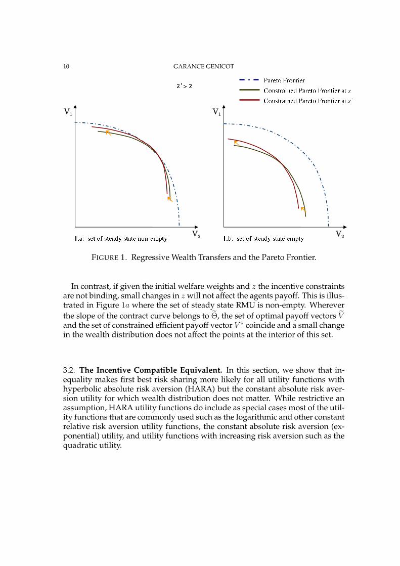
Figure 1b provides a graphical description of Proposition 2. The set of optimalpayoff vectors V is represented with a dashed line while the sets of constrainedefficient payoff vectors V ∗ for two different wealth allocations z = 1/2 and z′ > z

are represented with solid lines. V lies everywhere above V ∗(1/2), since the setof steady state RMU is empty at z = 1/2, and the lowest possible implementableexpected utility for an agent at date 0 corresponds to his autarchic utility. Nowconsider a small transfer of wealth from 2 to 1 such that z′ > 1/2. We see that asz increases the frontier of the set of implementable payoff vectors pivots to theright.

10 GARANCE GENICOT

FIGURE 1. Regressive Wealth Transfers and the Pareto Frontier.

In contrast, if given the initial welfare weights and z the incentive constraintsare not binding, small changes in z will not affect the agents payoff. This is illus-trated in Figure 1a where the set of steady state RMU is non-empty. Whereverthe slope of the contract curve belongs to Θ, the set of optimal payoff vectors Vand the set of constrained efficient payoff vector V ∗ coincide and a small changein the wealth distribution does not affect the points at the interior of this set.

3.2. The Incentive Compatible Equivalent. In this section, we show that in-equality makes first best risk sharing more likely for all utility functions withhyperbolic absolute risk aversion (HARA) but the constant absolute risk aver-sion utility for which wealth distribution does not matter. While restrictive anassumption, HARA utility functions do include as special cases most of the util-ity functions that are commonly used such as the logarithmic and other constantrelative risk aversion utility functions, the constant absolute risk aversion (ex-ponential) utility, and utility functions with increasing risk aversion such as thequadratic utility.


Utility functions of the HARA class take the following shape:

u(c) =

{1−k

(2−k)γ[γc + β]

2−k1−k + C, if k 6= 1, 2;

ln(γc + β), if k = 2.

where γ1−k

< 0 and β > −γc for all c. Among these we can distinguish (a)utilities exhibiting decreasing risk aversion, k > 1 and γ > 0; and (b) utilitieswith increasing risk aversion, k < 1 and γ < 0. If k = 1, the utility correspondsto the case of constant absolute risk-aversion in which clearly there is no wealtheffect, and therefore redistribution of wealth will not affect the extent of risk-sharing. Hence, in what follows we focus on k 6= 1.

We claim that in this case, redistributing wealth from the poorest to the richestagent makes it more likely that the set of steady state RMU is non empty. Itis in this sense that inequality makes perfect insurance more likely. To makethis claim more precise, it will help to define the concept of incentive compatibleequivalent.

We saw that perfect insurance consists in keeping the ratio of marginal utili-ties – the relative needs – of the agents constant across all state of nature. Hence,to know whether perfect insurance is possible or not, we can compare the high-est constant RMU that would satisfy all of individual 1’s incentive constraintswith the smallest constant RMU that individual 2 would accept.

A ratio of marginal utility θ and aggregate resources y imply the followingconsumption level for i:

(11) ci = gi(θ, y) = xi(θ)y + (xi(θ)− x−i(θ))β

γfor i ∈ {1, 2}

for a pair of shares

(12) x1(θ) =1

1 + θk−1and x2(θ) =

θk−1

1 + θk−1(= 1− x1(θ)).

Clearly, it is when an agent’s income is the largest (her realized income shockof εN ) while the other agent’s income is the lowest (his income shock of ε1) thather incentive constraint is the hardest to satisfy. Let y = 1 + ε1 + εN and yi =

zi + εN . The largest constant RMU that individual 1 would accept θ is thereforeso that

(13) (1− δ)u(g1(θ, y)) + δEs′u(g1(θ, ys′)) = (1− δ)u(y1) + δua(z1).

12 GARANCE GENICOT

Similarly, the smallest constant RMU that satisfies all of 2’s incentive constraintθ is defined by

(14) (1− δ)u(g2(θ, y)) + δEs′u(g2(θ, ys′)) = (1− δ)u(y2) + δua(z2).

Perfect insurance is implementable if the highest RMU that 1 requires is lessthan the largest RMU that 2 wants: θ ≤ θ.

Individual i’s incentive compatible equivalents (ICE) is the constant share that justsatisfies all incentive constraints for this agent:

x1 = x1(θ) and x2 = x2(θ).

Notice that for the commonly used utility with constant relative risk aversion,as for utility functions where β = 0, the shares x correspond to the shares ofaggregate income allocated to the agents.

For the utilities of type (a) (decreasing risk aversion), an increase in xi trans-lates into an increase in i’s consumption. Hence, any x ≥ x1 would satisfy 1’sconstraints and 2 would accept any share x for 1 lower or equal to 1 − x2. Itfollows that the set of steady state RMUs is non empty if and only if x1 < 1− x2.In contrast, for utilities of type (b) an increase in xi decreases i’s consumption.Agent 1 would accept any x ≤ x1 and 2 can credibly commit to any share x for1 not smaller than 1 − x2. In this case, a steady state RMU exists if and only ifx1 > (1− x2).

Hence, define

∆x =

{x1 − (1− x2) if k > 1 and γ > 0(1− x2)− x1 if k < 1 and γ < 0

The following proposition says that increasing the richest agent’s share ofwealth decreases ∆x. In other words, a more equal wealth distribution makesperfect insurance less likely.

Proposition 3. If z

<=>

1/2 thend(∆x)

dz

>=<

0

Proposition 3 implies that if the set of steady state RMU is non-empty at z ≥1/2 then it is non-empty at z′ > z. And if the set is empty at some z ≥ 1/2then transferring wealth from 2 to 1 makes x1 and (1− x2) converge. Once theyhave converged then the set of steady state RMU is non-empty, that is perfectinsurance is possible and, for any initial welfare weights, the ratio of marginal


utilities of the agent converges to a constant. The following example and Figure2 illustrate this result.

Example 1. The incentive compatible equivalent.

In this example we assume a very simple income distribution for the agents thatwe will use again later. The agents’ fluctuating income can take only one oftwo values, h or ` with h > ` ≥ 0, with probability 1/2 each. The individuals’fluctuating income are perfectly negatively correlated (when one get h the othergets `), such that the aggregate income stays constant.Assume that our two individuals have constant relative risk aversion utility(CRRA):

u(c) =c1−ρ

1− ρ

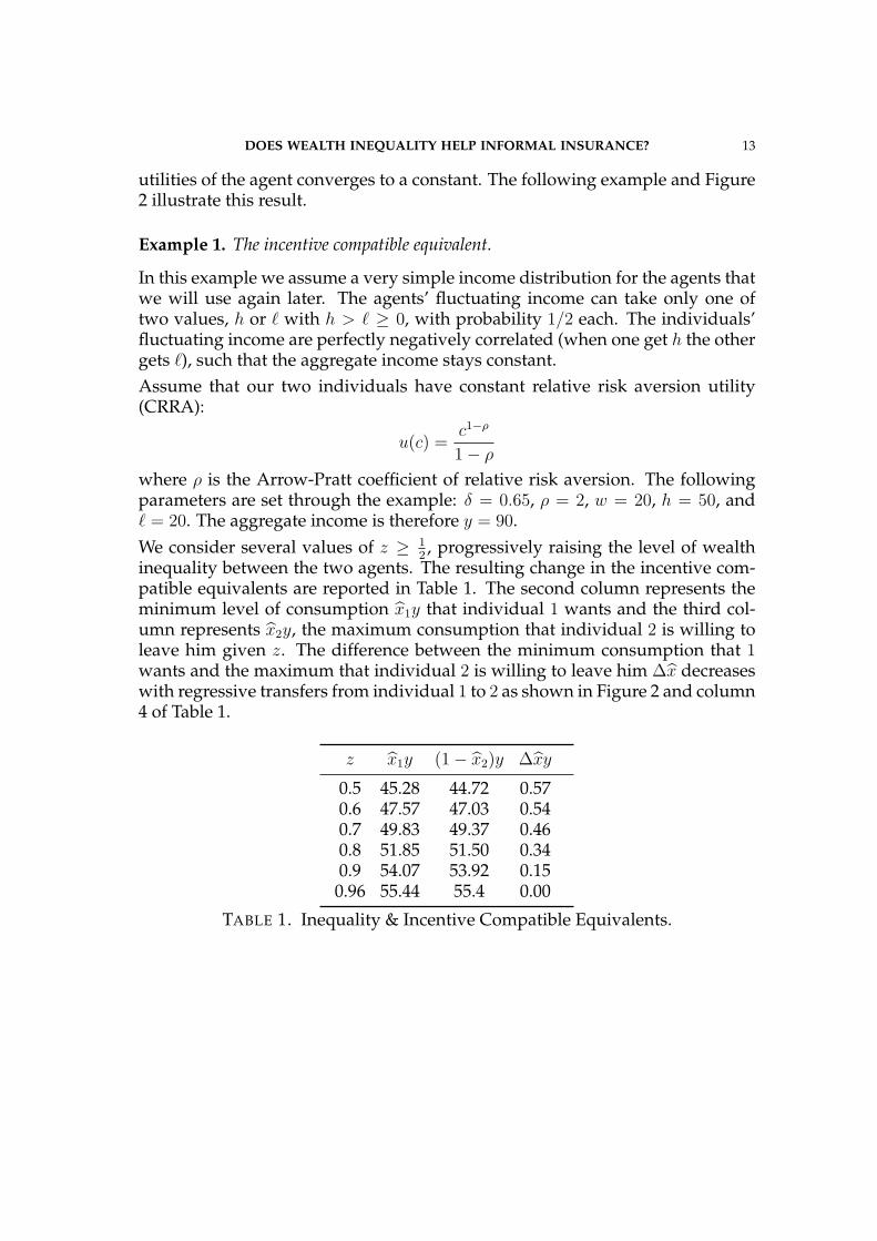
where ρ is the Arrow-Pratt coefficient of relative risk aversion. The followingparameters are set through the example: δ = 0.65, ρ = 2, w = 20, h = 50, and` = 20. The aggregate income is therefore y = 90.We consider several values of z ≥ 1

2, progressively raising the level of wealth

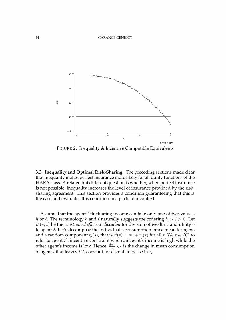
inequality between the two agents. The resulting change in the incentive com-patible equivalents are reported in Table 1. The second column represents theminimum level of consumption x1y that individual 1 wants and the third col-umn represents x2y, the maximum consumption that individual 2 is willing toleave him given z. The difference between the minimum consumption that 1wants and the maximum that individual 2 is willing to leave him ∆x decreaseswith regressive transfers from individual 1 to 2 as shown in Figure 2 and column4 of Table 1.

z x1y (1− x2)y ∆xy

0.5 45.28 44.72 0.570.6 47.57 47.03 0.540.7 49.83 49.37 0.460.8 51.85 51.50 0.340.9 54.07 53.92 0.15

0.96 55.44 55.4 0.00

TABLE 1. Inequality & Incentive Compatible Equivalents.

14 GARANCE GENICOT

dic

z

.4 .6 .8 1

-.2

0

.2

.4

.6

FIGURE 2. Inequality & Incentive Compatible Equivalents

3.3. Inequality and Optimal Risk-Sharing. The preceding sections made clearthat inequality makes perfect insurance more likely for all utility functions of theHARA class. A related but different question is whether, when perfect insuranceis not possible, inequality increases the level of insurance provided by the risk-sharing agreement. This section provides a condition guaranteeing that this isthe case and evaluates this condition in a particular context.

Assume that the agents’ fluctuating income can take only one of two values,h or `. The terminology h and ` naturally suggests the ordering h > ` > 0. Letc∗(v, z) be the constrained efficient allocation for division of wealth z and utility vto agent 2. Let’s decompose the individual’s consumption into a mean term, mi,and a random component ηi(s), that is ci(s) = mi + ηi(s) for all s. We use ICi torefer to agent i’s incentive constraint when an agent’s income is high while theother agent’s income is low. Hence, dmi

dzi|ICi

is the change in mean consumptionof agent i that leaves ICi constant for a small increase in zi.


A sufficient condition for the introduction of inequality to improve risk-sharingis that, keeping the transfer scheme unchanged

dm1

dz1

|IC1

<=>

dm2

dz2

|IC2 for all z

<=>

1/2.

The above condition requires the (spread-preserving) increase in mean con-sumption mi that keeps i’s incentive constraint unchanged for an increase in zi

to be smaller for the richest agent.

Clearly this condition is difficult to evaluate in the most general case. Hence,in this section, we study the relationship between wealth inequality and risksharing in the case where the aggregate income is constant, as in Example 1,since this case can be explicitly solved for. The agent’s labor income being sym-metric, this implies a probability 1/2 for each state. The following table summa-rizes the labor income distribution of the two agents.3

individual\state state1 state21 h `2 ` h

probability 1/2 1/2

It is well known that with this simple distribution, when no first best alloca-tion is incentive compatible, the constrained optimal agreement with the mostinsurance is fully characterized by two values, that we shall denote as c and c,individual 1’s consumption when his income is high and when his income islow. These consumption levels are such that the incentive constraints hold withequality,

(1− δ

2)u(c) +

δ

2u(c) = (1− δ

2)u(z + h) +

δ

2u(z + `)(15)

(1− δ

2)u(y − c) +

δ

2u(y − c) = (1− δ

2)u((1− z) + h) +

δ

2u((1− z) + `)

where y = 1 + ` + h is the aggregate income.

Proposition 4. For all utility functions of the HARA class with k ≥ 2 or k sufficientlyclose to 0, introducing some inequality between the agents when risk-sharing is notperfect improves informal insurance by reducing c− c.

3Note that the states are labeled for the agent whose income is high.

16 GARANCE GENICOT

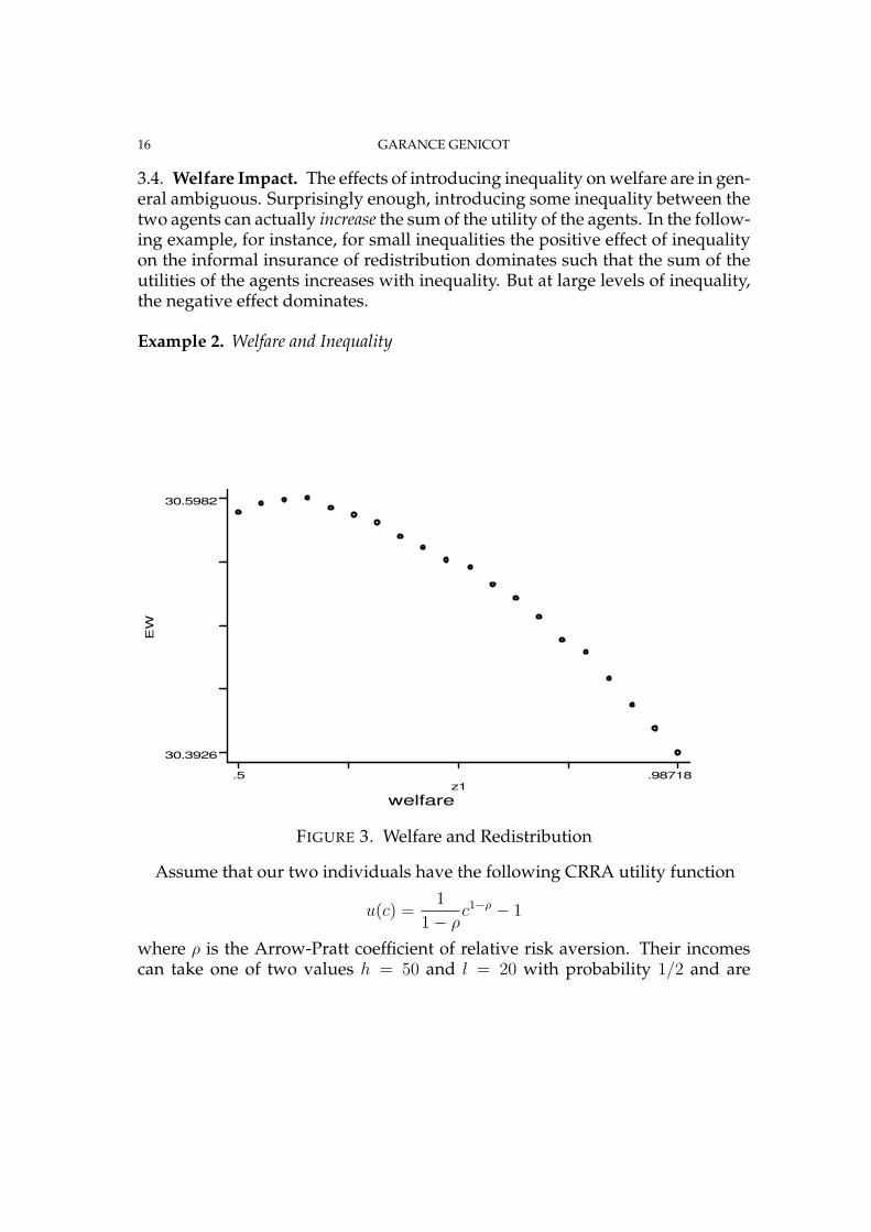
3.4. Welfare Impact. The effects of introducing inequality on welfare are in gen-eral ambiguous. Surprisingly enough, introducing some inequality between thetwo agents can actually increase the sum of the utility of the agents. In the follow-ing example, for instance, for small inequalities the positive effect of inequalityon the informal insurance of redistribution dominates such that the sum of theutilities of the agents increases with inequality. But at large levels of inequality,the negative effect dominates.

Example 2. Welfare and Inequality

EW

welfare

z1

.5 .98718

30.3926

30.5982

FIGURE 3. Welfare and Redistribution

Assume that our two individuals have the following CRRA utility function

u(c) =1

1− ρc1−ρ − 1

where ρ is the Arrow-Pratt coefficient of relative risk aversion. Their incomescan take one of two values h = 50 and l = 20 with probability 1/2 and are


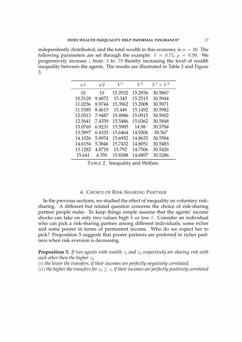
independently distributed, and the total wealth in this economy is w = 20. Thefollowing parameters are set through the example: δ = 0.75, ρ = 0.99. Weprogressively increase z from .5 to .78 thereby increasing the level of wealthinequality between the agents. The results are illustrated in Table 2 and Figure3.

w1 w2 V 1 V 2 V 1 + V 2

10 10 15.2932 15.2936 30.586710.5128 9.4872 15.343 15.2515 30.594411.0256 8.9744 15.3962 15.2008 30.597111.5385 8.4615 15.449 15.1492 30.598212.0513 7.9487 15.4986 15.0915 30.590212.5641 7.4359 15.5486 15.0362 30.584813.0769 6.9231 15.5985 14.98 30.578413.5897 6.4103 15.6464 14.9206 30.56714.1026 5.8974 15.6952 14.8632 30.558414.6154 5.3846 15.7432 14.8051 30.548315.1282 4.8718 15.792 14.7506 30.542615.641 4.359 15.8388 14.6897 30.5286

TABLE 2. Inequality and Welfare.

4. CHOICE OF RISK-SHARING PARTNER

In the previous sections, we studied the effect of inequality on voluntary risk-sharing. A different but related question concerns the choice of risk-sharingpartner people make. To keep things simple assume that the agents’ incomeshocks can take on only two values high h or low `. Consider an individualwho can pick a risk-sharing partner among different individuals, some richerand some poorer in terms of permanent income. Who do we expect her topick? Proposition 5 suggests that poorer partners are preferred to richer part-ners when risk aversion is decreasing.

Proposition 5. If two agents with wealth z1 and z2 respectively are sharing risk witheach other then the higher z2

(i) the lower the transfers, if their incomes are perfectly negatively correlated;(ii) the higher the transfers for z2 ≥ z1 if their incomes are perfectly positively correlated

18 GARANCE GENICOT

and the opposite for z2 < z1;

Proposition 5 shows that when the labor incomes are perfectly negatively cor-related, larger transfers are possible when agent 1 is paired with poorer agentsif risk aversion is decreasing. Keeping the transfers, between 1 and 2 the same,lowering 2’s wealth relaxes the incentive constraint. That is, a poorer 2 is willingto give more to 1 when high in exchange of the same transfer from 1 when he islow. The level of insurance is higher and they receive more surplus.

When incomes are perfectly positively correlated, agents with the same levelof permanent income are unable to provide insurance to each other. Largertransfers are possible only if agent 1 is matched with someone either sufficientlyricher or sufficiently poorer that some transaction occurs. If risk aversion isdecreasing the poorest of the two agents would borrow when both are low andrepay when both are high.

We could push the inquiry further and ask the question of which matcheswould form among different individuals, some rich and some poor. Assumingthat individuals share risk in pairs (see Genicot and Ray 2003, 2005 for reasonsfor which small groups form), who do we expect to see sharing risk with eachother? This is related to Ghatak (1999) and Sadoulet (2001) who look at pairwisematching in group lending in the presence of heterogeneity in risk.4

Consider a very simple example: two sets of agents M and F of same size– male and female say – can form pairs to share risk with each other. Assumethat each set contains two agents, a poor with wealth zp and a rich with wealthzr (zr > zp), and that individuals have decreasing risk aversion. In this case,the matching that we expect to observe depends on the correlation between theincomes of the two set of agents.

Proposition 6. [i] Positive assortative matching is stable if incomes are perfectly posi-tively correlated; and [ii] negative assortative matching is stable with perfectly positivelycorrelated incomes;

Notice that this proposition relies on stationary contracts. Allowing for his-tory dependent contract – described in details in Section – we would not neces-sarily get positive assortative matching when incomes are perfectly negativelycorrelated. Proposition 5 tells us that poorer individuals are willing to makelarger transfers when low in exchange of a given transfer when rich. This is

4Also clearly relevant is Legros and Newman (2002) who study monotonic matching in thecontext of non-transferable utilities.


why we expect that the poorer agents would be better off forming a risk sharingagreement among themselves. However this is not necessarily the case. It isrelatively easier for richer agents to temporarily demand a lower transfer fromthe poorer agent if the latter is high as long as he has not received `. As soonas the poorer agent receives `, the agreement consists in the larger transfers thatthe two agents incentive constraints allow. Hence, the stability of a match is acomplex object to check for as the following example illustrates.

Example 3. Endogenous Matching

Individuals have CRRA utilities u(c) = 11−ρ

c1−ρ with risk aversion ρ = 0.8 anddiscount rate δ = 0.8. Their labor incomes can be low ` = 1 or high h = 3 withprobability 1/2 and are perfectly negatively correlated between the two M andF .

Let the poor’s wealth zp be 1. Denote as upp the expected utility (in per periodterm) that a poor person has when sharing risk in a symmetric agreement withsomeone of same wealth and as urr the same object for a rich person. A matchwhere poor and rich are sharing risk in separate groups is stable if there is norisk-sharing agreement between a poor and rich that could give to at least upp tothe poor and urr to the rich.

In our example, this the case for relatively small difference between poor andrich. If zr = 1.5, there is no agreement between a rich and a poor that can giveat least upp = 6.42 to the poor while guaranteeing urr = 6.59. In contrast, if therich are twice as wealthy as the poor zr = 2, then by giving the poor a breakearly on in the relationship, the rich can guarantee an expected utility of at leastupp = 6.42 to the poor while earning more than urr = 6.75.

5. IMPLICATIONS, LIMITATIONS AND EXTENSIONS

The remainder of the paper explores some important extensions and policyimplications of the previous results.

5.1. Income Inequality and Consumption Inequality. Krueger and Perri (2002)investigate the relationship between the cross-sectional distribution of incomeand consumption in the United States between 1980 and 1997. They present ev-idence that the Gini coefficient of after-tax labor income did increase while theconsumption Gini remained roughly constant.

20 GARANCE GENICOT

The authors suggest that an increase in the spread in the agent’s income dis-tribution is a potential explanation for this observation. They consider the spe-cific two-agent example with perfectly negatively correlated income, similar toExample 1. The agents have constant relative risk aversion and their incomedistributions are multiple of each other. They show that in this case, when risk-sharing is not perfect, an increase in the dispersion in the agents’ income in-creases both the Gini measure of income inequality and the level of risk-sharingamong the agents.5 An increase in income dispersion would then result in alower increase in the consumption Gini than in the income Gini.

Evidences show that the US income distribution experienced both a perma-nent increase in inequality and an increase in the dispersion in the personalincome distribution (see Katz and Autor (1999) for a review of these evidences).Hence, this paper suggests another channel through which higher inequalityin income, by increasing the level of voluntary risk-sharing, could actually de-crease the inequality in consumption.

5.2. Redistribution Program. To be sure, these results have policy implicationsregarding redistribution programs. One of the most important redistributionpolicy being land reform.

Redistribution is of course a goal in itself, quite apart from any efficiency gainsthat might result from a more equitable land distribution. However as many re-cent papers have argued, inequality can have positive as well as negative effectsof efficiency. In this paper, we identified a new potential cost of redistribution.In many cases, redistribution reduces the level of risk-sharing or informal insur-ance to which people have access.

In example 2, we saw a situation where introducing some inequality actuallyincreased the sum of the utilities of the agents. In such situation, even a gov-ernment that slightly favors the poorest agent may actually side with the richestagent and oppose a land reform. This is because the loss of efficiency due to adecrease in risk-sharing dominates the benefits from redistribution. If the initialinequality is very large, then clearly the overall benefits or redistribution willdominate but it is still important to realize that the level of insurance may havedecreased in the process.

Naturally, if the redistribution that takes place, such as land reform, effec-tively increases the access of the poor to formal forms of credit then this would

5Note that with two income shocks, this result can be shown to hold whenever stationaryschemes are feasible and self-enforcing.


mitigate the consequences of the loss of informal insurance. Otherwise redistri-bution initiatives should be accompanied by safety net policies.

6. CONCLUSION

Need to provide better insurance

7. APPENDIX

7.1. The Constrained Optimal Allocation. Denote t-history as st ∈ St, that isthe history of all past and current realization of the state of nature up to time t.If we allow for history dependent risk-sharing arrangement, then an allocationis a list of functions σ = {ct}∞t=0 such that for all t ≥ 0, ct maps the product of t-histories and current income realizations to feasible consumption vectors. (nonnegative and for all t-history st ∈ St,

∑i c

it(s

t) ≤ ∑yi

st∀t, st).

Kocherlakota (1996) showed that the constrained optimal scheme depends onhistory in a very simple way. At any point in time, the current promise utilityto agent 2 summarizes all past history. For a given wealth distribution z, theconstrained optimal allocations solve the following maximization for differentvalues of v2,6

(16) v1(v2, z) = maxcs,v′s

Es

[(1− δ)u(c1(s)) + δv1(v

′s, z)

],

subject to the promise keeping constraint

(17) Es

[(1− δ)u(c2(s)) + δv′s

] ≥ v2,

feasibility and the individual’s incentive constraints:

(1− δ)u(c1(s)) + δv1(v′s, z) ≥ (1− δ)u(y1(s)) + δua(z1)(18)

(1− δ)u(c2(s)) + δv′s ≥ (1− δ)u(y2(s)) + δua(z2)(19)

for every state s and history v2.

Hence, denote as θ(st) the equilibrium ratio of marginal utilities (RMU) given st

θ(st) =u′(c1

t (st))

u′(c2t (s

t)).

6See Kocherlakota (1996) and Ligon et al. (2000).

22 GARANCE GENICOT

The first order condition for the problem tells us that

θ(st) =χ(st−1) + ψ2(st)

1 + ψ1(st)(20)

dv1(v′s, z)

dv2

= θ(st)(21)

where χ(st−1) is the multiplier on the promise keeping constraint (17), and p(st)ψi(st)

is the multiplier on i’s incentive constraint (18) or (19)given the realized state st.

It follows that the optimal contract is characterized by a simple updating rulefor the evolution of the ratio of marginal utilities along the equilibrium path. Ifno incentive constraint binds then the RMU at time t stays the same as last pe-riod realized RMU. Alternatively, if one individual’s incentive constraint bindsthe the ratio of marginal changes in the direction that relaxes the constraint, theleast as possible but enough to satisfy the binding incentive constraint.

Let θs(z) be the largest implementable RMU in state s — that is the largestRMU such that 1’s incentive constraint is not violated — given the efficientrisk-sharing agreement and wealth distribution z. Similarly, define θs(z) as thesmallest implementable RMU in state s — that is the smallest RMU such that 2’sincentive constraint is not violated. Let Θs(z) ≡ [θs(z), θs(z)] for all s ∈ S.7

Given a realized RMU θ(st−1) a time t − 1 the constrained efficient allocationis such that today’s RMU θ(st) follows the following law of motion

θ(st−1, s) =

θs(z)θ(st−1)θs(z)

for all s such that θ(st−1)

> θs(z)∈ Θs(z) ≡ [θs(z), θs(z)]< θs(z)

with θ(s−1) = 1−αα

.

Note that the current RMU is the absolute value of the slope of the contractcurve at the continuation utilities. A given θ(st−1) and the above updating ruleperfectly identifies the level of expected utility of the agents. When an agent’sconstraint binds, his continuation utility increases and the position on the con-tract curve is modified in a direction more favorable to this agent.

7Note that these concepts can be defined since the constraints are forward looking.


7.2. Proofs .

Proof of Proposition 1.Proof. Because the planner’s problem has a unique solution for every v2, thissolution must be continuous in the parameter z. It therefore suffices to consideronly changes in z from z to z′ such that exactly the same constraints bind beforeand after. The absolute value of that slope of the constrained Pareto frontier atv2 is given by the multiplier on the promise keeping constraint χ. To prove theProposition, we claim that following an increase from z to z′, the slope of theconstrained Pareto frontier χ has strictly increased for all v2 so that v1 has notincreased, v1(v2, z

′) ≤ v1(v2, z′). Assume that this claim is not true and that χ has

(weakly) decreased.Since an increase in z increases the right-hand-side of 1’s incentive constraint(6) and that v1(v2, z) has not increased, it must be that c1(s) strictly increase inall state s in which 1’s constraint binds. Similarly, an increase in z decreases theright-hand-side of 2’s incentive constraint (7) and v2(α, z) has increased, so thatc1(s) must strictly increase in all state s in which 2’s constraint binds.Finally, in all state s in which no incentive constraint binds, the first order con-dition (8) tells us that

u′(c1(s))

u′(ys − c1(s))= M≡ χ + δM2

1 + δM1

.

where Mi =∑

s′ µis′ . Let ∆Mi be the change in Mi and ∆χ be the change in χ

from z to z′.

Since v2 is the same and v1 has not increased, it must be the case that, in stateswhere no constraint binds, M has increased so that c1(s) decreases and c2(s)increases. Hence,

(22) (∆χ + δ∆M2)(1 + δM1)− δ∆M1(χ + δM2) ≥ 0.

Since ∆χ ≤ 0, this implies that either [a] ∆M2 ≥ 0 or [b] dM1 ≤ 0 or [c] both.

For all states s in which 2’s constraint binds, this, along with the first ordercondition (8) and the fact that c1(s) strictly increases, also implies that µ2

s/(1 +δM1) decreases. Hence,

(23) δ∆M2(1 + δM1)− δ∆M1(δM2) < 0.

Similarly, the first order condition (8) and the fact that c1(s) strictly increasesimply that µ1

s/(χ + δM2) increases for all states in which 1’s constraint binds. It

24 GARANCE GENICOT

follows that,

(24) (∆χ + δ∆M2)δM1 − δ∆M1(χ + δM2) < 0.

Notice that hypothesis [c], both ∆M2 ≥ 0 and dM1 ≤ 0, would immediatelycontradict inequalities (23) and (24) and therefore cannot be true.

Now, suppose that [b] holds so that ∆M2, ∆M1 ≤ 0. Notice that (22) and 24imply that

(∆χ + δ∆M2) ≥ δ∆M1(χ + δM2)− (∆χ + δ∆M2)δM1 > 0.

This is a contradiction, since under [a] the left-hand side is strictly negative.

Finally, assume that [a] holds so that ∆M2, ∆M1 ≥ 0. Inequalities (22) and 23jointly imply that

∆χ(1 + δM1)− χδ∆M1 ≥ δ∆M1(δM2)− δ∆M2(1 + δM1) > 0.

But, [a] implies that the left-hand-side is negative, a contradiction.

This contradicts the initial hypothesis that χ has not increased. Hence, theslope of the constrained Pareto frontier must strictly increase whenever whenv1(v2, z

′) ≤ v1(v2, z) so that we have a single crossing.

Proof of Proposition 2. The effect of a small change in z on the LagrangianL(v2; z) is given by

dL(v2; z)

dz= −∑

s µ1(s)[u′(z + ε1(s)) + δ

1−δ

∑s′ p(s′)u′(z + ε1(s′))] +

∑s µ2(s)[u

′((1− z) + ε2(s)) + δ1−δ

∑s′ p(s′)u′((1− z) + ε2(s′))]

since by the envelope theorem all derivatives of Lwith respect to µi(s) and ci(s)are null.

At z = 1/2, both individuals are exactly identical and the income distributionsare symmetric so that for each state s where 1’s constraint is binding there is asymmetric state s with µ1(s) = µ1(s

′) and u′(y1(s))+ δ1−δ

Eu′(y1(s′)) = u′(y2(s))+

δ1−δ

∑s′ p(s′)u′(y2(s

′)). Hence dv1(v1, 1/2)/dz = 0.

This in combination with Proposition 1, imply thatdv1(v; 1

2)

dz< 0 for v > v1

whiledv1(v; 1

2)

dz> 0 for v < v1.


Proof of Proposition 3.Recall that given our utility function,

u(gi(θ, Y )) =(1− k)

(2− k)γ[xi(θ)(γY + 2β)]

2−k1−k .

Using this in the definition of θ in (13) and θ in (14), we can rewrite x1 = x1(θ)and x2 = x2(θ) as

(25) xi =

[(1− δ)[xa

i (γy + 2β)]2−k1−k + δEs[x

ai (s)(γYs + 2β)]

2−k1−k

(1− δ)(γy + 2β)2−k1−k + δEs(γYs + 2β)

2−k1−k

] 1−k2−k

where xai = γ(zi+εN )

γey+2βand xa

i (s) = γ(yi(s))γYs+2β

are the autarchic shares.

Since dxai (s)

dzi= γ

γys+2β, the effect of a small increase in z on x1 is given by

(26)dxi

dzi

=γBi

[Oi]1−k2−k [Ai]

12−k

where

Ai = [xai (γy + 2β)]

2−k1−k + δ

1−δEs[x

ai (s)(γYs + 2β)]

2−k1−k ;

Bi = [xai (γy + 2β)]

11−k + δ

1−δEs[x

ai (s)(γYs + 2β)]

11−k ;

Oi = (γy + 2β)2−k1−k + δ

1−δEs(γYs + 2β)

2−k1−k .

Two observations directly follow from this equation. First, an increase in 1’sshare of wealth increases the levels of consumption corresponding to 1’s ICEand decreases the level of consumption corresponding to 2’s ICE. So the ques-tion is which of these effects dominates. Second, at z = 1/2, the effects on 1’sICE and 2’s ICE just cancel out, that is d(bx1+bx2)

dzjust equals zero.

Hence, to prove our claim it suffices to show that xi is concave in z for the utilityfunctions of type (a) and convex for the utilities of type (b).

Taking the derivative of (26), we find that(27)

d2xi

d(zi)2=

[Ai]1−k2−k

−2

[Oi]1−k2−k

γ2 11−k

[xa

i (γy + 2β)]k

1−k + δ1−δ

Es[xai (s)(γys + 2β)]

k1−k

]Ai −B2

i

26 GARANCE GENICOT

Since 11−k

is negative for the utility of class (a) but positive for the utilities ofclass b, it follows that the proposition is true if[xi(γy + 2β)]

k1−k + δ

1−δEs[xi(s)(γys + 2β)]

k1−k

] [[xi(γy + 2β)]

2−k1−k + δ


2−k1−k

]

≥[[xi(γy + 2β)]

11−k + δ


11−k

]2

Expanding both sides of the inequality, we see that

[xi(γy + 2β)]2

1−k + δ1−δ

Es[xi(s)(γys + 2β)]2

1−k + δ1−δ

[xi(γy + 2β)]k

1−k Es[xi(s)(γys + 2β)]2−k1−k

+ [xi(γy + 2β)]2−k1−k δ


k1−k + 2( δ

1−δ)2EsEs′>s[xi(s)(γys + 2β)]

k1−k

[xi(s′)(γYs′ + 2β)]

2−k1−k ≥ xi(γy + 2β)]

21−k + δ


21−k + 2

[xi(γy + 2β)]1

1−k δ1−δ

Es[xi(s)(γys + 2β)]1

1−k + 2( δ1−δ

)2EsEs′>s[xi(s)(γys + 2β)]1

1−k

Canceling some terms, we can rewrite this last inequality as

Es[xi(s)(γys + 2β)]k

1−k [xi(s)(γys + 2β)− xi(γy + 2β)]2 δ1−δ

[xi(γy + 2β)]k

1−k + ( δ1−δ

)2

EsEs′>s[xi(s)(γys + 2β)xi(s′)(γYs′ + 2β)]

k1−k [xi(s)(γys + 2β)− xi(s

′)(γYs′ + 2β)]2 ≥ 0

which is clearly satisfied.

Proof of Proposition 4. Before we proceed to a proof of Proposition 4, the fol-lowing preliminary lemma is useful.

Lemma 1. For all utility functions of the HARA class with k ≥ 2 or k sufficiently closeto 0, and for any two values c and c such that c > c, increasing the insurance along theincentive constraint decreases the following expression:

(28)−(1− δ

2)u′′(c)− ( δ

2)u′′(c)[

(1− δ2)u′(c) + ( δ

2)u′(c)

]2 .

Proof. Moving along the incentive constraint means that (1 − δ2)u(c) + ( δ

2)u(c)

remains constant. Hence, increasing the level of insurance along the constraint

means that a unit decrease in c is compensated by an increase in c of(1− δ

2)

δ2

u′(c)u′(c) .


A simple differentiation tells us that, for utility functions of the HARA class, theeffect of such changes on (28) is negative if

−γ1−k

2(1− δ2)

[[γc + β]

k1−k

[γc+βγc+β

] 11−k − [γc + β]

k1−k

][(1− δ

2)[γc + β]

k1−k + δ

2[γc + β]

k1−k

]

< −γk1−k

(1− δ2)

[[γc + β]

k1−k

−1[

γc+βγc+β

] 11−k − [γc + β]

k1k−1

] [(1− δ

2)[γc + β]

11−k + δ

2[γc + β]

11−k

].

Simplifying this expression we get

2 [γc+β]

k1−k

[γc+β][[γc + β]− [γc + β]]

[(1− δ

2)[γc + β]

k1−k + δ

2[γc + β]

k1−k

]

< k [γc+β]

k1−k

−1

[γc+β]2[[γc + β]2 − [γc + β]2]

[(1− δ

2)[γc + β]

11−k + δ

2[γc + β]

11−k

],

which, on rearrangement, yields

(2− k)[γc + β][γc + β]γ(c− c)

[(1− δ

2)[γc + β]

k1−k + δ

2[γc + β]

k1−k

]

< kγ(c− c)

[(1− δ

2)[γc + β]

11−k + δ

2[γc + β]

11−k

].(29)

Remember that γ1−k

is negative such that either γ > 0 and k > 1 decreasingabsolute risk aversion) or γ < 0 and k < 1 (increasing absolute risk aversion),while the special case of k = 1 corresponds to constant absolute risk aversion. Itis easy to check that for all k ≥ 2 and at k = 0 (quadratic utility), the inequality(29) is satisfied. This establishes the lemma. Note that this inequality is violatedfor values of k close to 1.

We now complete the proof of the proposition. To this end, differentiating (15),we see that

[(1− δ

2)u′(c) δ

2u′(c)

− δ2u′(y − c) −(1− δ

2)u′(y − c)

] [dc/dzdc/dz

]=

[ω(z)

−ω(1− z)

]

where

ω(zi) = (1− δ2)u′(zi + h) + δ

2u′(zi + `).

and therefore,

28 GARANCE GENICOT

dc

dz=

1

D

[−(1− δ

2)u′(y − c) ω(z) +

δ

2u′(c) ω(1− z)

](30)

dc

dz=

1

D

[−(1− δ

2)u′(c) ω(1− z) +

δ

2u′(y − c) ω(z)

](31)

where D = −(1− δ2)2u′(c)u′(y − c) + ( δ

2)2u′(c)u′(y − c).

It is easy to show that D < 0 since otherwise it would be possible to find avector of consumption providing more insurance to the agents while satisfyingtheir incentive constraints. Note also that either c or c or both increases as 1’sshare of wealth z increases, and therefore at z = 1/2 both c and c increase.

Inequality improves insurance, that is to decrease the spread between c and c, ifthe following is true:

(32)d(c− c)

dz

> 0 if z < 12,

= 0 if z = 12,

< 0 if z > 12

The sign ofd(c− c)

dzis given by the sign of

ω(z)

(1− δ2)u′(c) + δ

2u′(c)

− ω(1− z)

(1− δ2)u′(y − c) + δ

2u′(y − c)

Hence, our claim requires that the (spread preserving) increase in mean con-sumption that keeps agent 1’s incentive constraint unchanged after an increasein her wealth be less that the decrease in mean consumption that agent 2’s in-centive constraint would allow following a decrease in his wealth.

A sufficient condition for (32) to be true is that

(1− δ2)u′(z + h) + δ

2u′(z + `)

(1− δ2)u′(c) + δ

2u′(c)

decreases in z (note that c and c both depend on z). That is,

(33)−(1− δ

2)u′′(z + h)− δ

2u′′(z + `)

(1− δ2)u′(z + h) + δ

2u′(z + `)

>−(1− δ

2)u′′(c) dc

dz− δ

2u′′(c) dc

dz

(1− δ2)u′(c) + δ

2u′(c)

.

At z = 1/2, it is easy to see that

dcdz

= dcdz

=(1− δ

2)u′(z + h) + δ

2u′(z + `)

(1− δ2)u′(c) + δ

2u′(c)


Hence, starting from a situation of perfect equality, a regressive transfer in per-manent income necessarily improves insurance if

−(1− δ2)u′′(z + h)− δ

2u′′(z + `)[

(1− δ2)u′(z + h) + δ

2u′(z + `)

]2 >−(1− δ

2)u′′(c) dc

wdz− δ

2u′′(c) dc

wdz[(1− δ

2)u′(c) + δ

2u′(c)

]2

This inequality together with lemma (1) completes the proof of the proposition.

Proof of Proposition 5: To prove this claim, the following lemma is useful.

Lemma 2. Pick two consumption level c and c and let v(c, c) = pu(c)+qu(c). If c > c,a small reduction in c compensated by an increase in c keeping v(c, c) constant decreases(increases) the following expression,

(34) pu′(c) + qu′(c),

for all utility functions with decreasing (increasing) risk aversion. The converse is trueif c < c.

Proof. Consider a small decrease in c compensated by an increase in c thatkeeps v(c, c) constant. That is −pu′(c)dc + qu′(c)dc = 0 or dec

dc= pu′(c)

qu′(ec) . A simpledifferentiation shows that the effect of such changes on the expression (34) isnegative (positive) if

−pu′′(c)dc + qu′′(c)dc < (>) 0

−u′′(c)u′(c)

+u′′(c)u′(c)

< (>) 0

If the utility function exhibits decreasing risk aversion, the left hand side ofthis inequality is negative (positive) if c > c (c < c). Clearly the converse is trueif risk aversion is increasing.

Consider part (i) of the claim. When the agents’ incomes are perfectly nega-tively correlated, they are recipients of transfers when their income is low andgive transfers when their income is high. Let c and c be agent 2’s consumptionwithin the risk-sharing agreement in the state where his income is high and lowrespectively. If the incentive constraint binds z2 + ` < c < c < z2 + h and

(1− δ2)u(c) + ( δ

2)u(c) = (1− δ

2)u(z2 + h) + ( δ

2)u(z2 + `).

30 GARANCE GENICOT

Notice that we can find get from (z2 + h, z2 + `) to (c, c) using a sequence ofsmall changes in ch and cl that decreases the spread and keeps (1 − δ

2)u(ch) +

( δ2)u(cl) constant. Hence, together with Lemma 2, it implies that

(1− δ2)u′(c) + ( δ

2)u′(c) < (1− δ

2)u′(z2 + h) + ( δ

2)u′(z2 + `).

So that, following an increase in z2, the same transfers between 1 and 2 do notsatisfy 2’s incentive constraint. The increase in z2 reduces the transfer that agent2 is willing to make when his income is high for any given transfer that agent 1makes in return. As a result, the higher z2 the lower the level of insurance.

Now, let’s turn to part (ii) of the claim. It is easy to see that a necessary andsufficient condition for i making a non-zero transfers to j when `` occurs is that

(35)

(1− δ

2δ2

)2

≤ θauthh

θaut``

where θaut is the ratio of marginal utilities of i to j in autarchy.

Indeed, (35) is condition for the maximum price for a unit transfer when low

that j is willing to pay when highδ2

1− δ2

u′(zj+`)

u′(zj+h)to be greater or equal to the mini-

mum that i would want to make such transfer1− δ

2δ2

u′(zi+l)u′(zi+h)

.

Clearly, a necessary condition for (35) to hold is that θauthh > θaut

`` . Clearly, notransfer is possible when z1 = z2. When risk aversion is decreasing (increas-ing), θaut

hh /θaut`` requires zi > zj (zi < zj) to be larger than 1 and is increasing in zi

and decreasing in zj (decreasing in zi and increasing in zj). With decreasing (in-creasing) risk aversion, the poorer (richer) agent would receive a transfer when`` occurs and gives a transfer when hh is realized. Moreover, the difference inwealth between the two agents needs to be sufficiently large for transfers to bepossible.

Assume that a non-zero transfer is possible and zi > zj . Let cj and cj be j’sconsumption when `` and hh respectively. If risk aversion is decreasing thenzj + ` < cj < cj < zj + h while ci < zi + ` < zi + h < ci. Moreover

(1− δ2)u(cj) + ( δ

2)u(cj) = (1− δ

2)u(zj + h) + ( δ

2)u(zj + `);

(1− δ2)u(ci) + ( δ

2)u(ci) = (1− δ

2)u(zi + `) + ( δ

2)u(zi + h).


Using lemma 2, we see that

(1− δ2)u′(cj) + ( δ

2)u′(cj) < (1− δ

2)u′(zj + h) + ( δ

2)u′(zj + `);

(1− δ2)u′(ci) + ( δ

2)u′(ci) > (1− δ

2)u′(zi + `) + ( δ

2)u′(zi + h).

It follows that given the same transfers between 1 and 2, a decrease in zj or anincrease in zi relaxes the incentive constraints. A similar argument can be usedfor utility functions with increasing risk aversion.

Proof of Proposition 6.Part [ii] is obvious in the view of Proposition 5 as homogenous agents are unableto provide each other any insurance. Hence, individuals can only be made betteroff by pairing up with someone of different wealth.

Now consider part [i]. Following Legros and Newman (2006), to check whetherpositive assortative matching is stable, we can focus on individuals of symmet-ric arrangement between individuals of same wealth. Let uzz be the utility of anindividual, agent 1, with wealth z in an homogenous match. Consider agent 2with wealth z′ > z. In order to attract agent 1 to form a match with her, agent 2needs to offer a contract (c, c) that guarantees 1 at least uzz. Let t1 = z + h− c bethe transfer that 1 gives when high and t2 = c− (z + `) the transfer she receiveswhen low. We saw in Proposition 5 that for any t1, a richer agent 2 cannot offeras high a t2 than a poorer agent. This implies that all contracts that between 1and 2 that are incentive compatible will have lower transfers than the transfersthat 2 would give and receive in a homogenous match. Since 1’s utility must beat least uzz this implies that t1 > t2 in a match between 1 and 2. Hence, agent2 would prefer the highest transfers (t1, t2) that gives uzz to 1 and satisfies hisincentive compatibility constraint if there is any. In this case, it follows that hisincentive constraint is binding

(1− δ

2)u(z′ + h− t1) +

δ

2u(z′ + ` + t2) = (1− δ

2)u(z′ + h) +

δ

2u(z′ + `).

Since t1 > t2, then t1, t2 < tz′ where tz′ is the transfer that 2 would make andreceive in a homogenous match

(1− δ

2)u(z′ + h− tz′) +

δ

2u(z′ + ` + tz′) = (1− δ

2)u(z′ + h) +

δ

2u(z′ + `).

Therefore, agent 2 could not guarantee uzz to 1 and receive a higher utility thanhis own utility in a homogenous match uz′z′ .

32 GARANCE GENICOT

REFERENCES

Aghion, P. and P. Bolton, “A Trickle-Down Theory of Growth andDevelopment,” Review of Economic Studies, 1997, 64, 151–162.

Alesina, A. and D. Rodrik, “Distributive Politics and Economic Growth,”Quarterly Journal of Economics, 1994, 109, 465–490.

Attanasio, O. and S. Davis, “Relative Wage Movements and the Distribution ofConsumption,” Journal of Political Economy, 1996, 104, 1227–62.

Banerjee, A. and A. Newman, “Occupational Choice and the Process ofDevelopment,” Journal of Political Economy, 1993, 101, 274–298.

Bertola, G., “Factor Shares and Savings in Endogenous Growth,” AmericanEconomic Review, 1993, 83, 1184–1198.

Bourguignon, F., “Pareto Superiority of Unegalitarian Equilibria in StiglitzModel of Wealth Distribution with Convex Saving Function,” Econometrica,1981, 49(6), 1469–75.

Coate, S. and M. Ravallion, “Reciprocity without Commitment:Characterization and Performance of Informal Insurance Arrangements,”Journal of Development Economics, 1993, 40(1), 1–24.

Deaton, A., “Understanding Consumption,” 1992.Foster, A. and M. Rosenzweig, “Imperfect Commitment, Altruism, and the

Family: Evidence from Transfer Behavior in Low-Income Rural Areas,”Review of Economics and Statistics, 2002, 83, 389–407.

Galor, 0. and J. Zeira, “Income Distribution and Macroeconomics,” Review ofEconomic Studies, 1993, 60, 35–52.

Genicot, G. and D. Ray, “Endogenous Group Formation in Risk-SharingArrangements,” Review of Economic Studies, 2003, 70(1), 87–113.

Gertler, P. and J. Gruber, “Insuring Consumption Against Illness,” AmericanEconomic Review, 2002, 92, 51–70.

Ghatak, M., “Group Lending, Local Information and Peer Selection,” Journal ofDevelopment Economics, 1999, 60(1), 229–248.

Grimard, F., “Household Consumption Smoothing through Ethnic Ties:Evidence from Cote D’Ivoire,” Journal of Development Economics, 1997, 53,391–422.

Jalan, J. and M. Ravallion, “Are the Poor Less Well Insured? Evidence onVulnerability to Income Risk in Rural China,” Journal of DevelopmentEconomics, 1999, 58, 61–81.

Katz, L. and D. Autor, Changes in the Wage Structure and Earnings Inequality,Vol. 3A, Amsterdam: North-Holland, 1999.

Kimball, M., “Farmers’ Cooperatives as Behavior Toward Risk,” AmericanEconomic Review, 1988, 78(1), 224–32.

References 33

Kletzer, K. and B. Wright, “Sovereign Debt as Intertemporal Barter,” AmericanEconomic Review, 2000, 90, 621–639.

Kocherlakota, N., “Implications of Efficient Risk Sharing withoutCommitment,” Review of Economic Studies, 1996, 63(4), 595–609.

Krueger, D. and F. Perri, “Does Income Inequality Lead to ConsumptionInequality? Evidence and Theory,” NBER working paper, 2002, 9202.

Legros, P. and A. Newman, “Assortative Matching with Nontransferabilities,”Review of Economic Studies, 2002, 69(4), 925–42.

Ligon, E., J. Thomas, and T. Worrall, “Mutual Insurance, Individual Savings,and Limited Commitment,” Review of Economic Dynamics, 2000, 3(3), 1–47.

Morduch, J., “Between the Market and State: Can Informal Insurance Patch theSafety Net?,” World Bank Research Observer, 1999, 14 (2), 187 – 207.

Murgai, R., P. Winters, E. Sadoulet, and A. de Janvry, Journal of DevelopmentEconomics, 2002.

Persson, T. and G. Tabellini, “Is Inequality Harmful for Growth?,” AmericanEconomic Review, 1994, 84, 600–621.

Posner, R., The Economics of Justice, Cambridge: Harvard University Press, 1981.Sadoulet, L., “Equilibrium Risk-Matching in Group Lending,” Technical

Report 2001.Townsend, R., “Risk and Insurance in Village India,” Econometrica, 1994, 62(3),

539–91.Udry, C., “Risk and Insurance in a Rural Credit Market: An Empirical

Investigation in Northern Nigeria,” Review of Economic Studies, 1994, 61(3),495–526.

does wealth inequality help informal insurance?

Documents