Does structure influence growth? A panel data econometric assessment

of ‘relatively less developed’ countries, 1979-2003

Ester Gomes da Silva

(esilva@letras.up.pt)

Faculdade de Letras/ISFLUP

Universidade do Porto

Aurora A. C. Teixeira

(ateixeira@fep.up.pt)

CEF.UP, Faculdade de Economia

Universidade do Porto, INESC Porto

Abstract

Neo-Schumpeterian streams of research emphasize the close relationship between

changes in economic structure in favour of high-skill and high-tech branches and rapid

economic growth. They identify the emergence of a new technological paradigm in the

1970s, strongly based on the application of information and communication

technologies (ICTs), arguing that in such periods of transition and emergence of new

techno-economic paradigms the relatively less developed countries have higher

opportunities to catch-up. Although this debate is theoretically well documented, the

empirics seem to lag behind the theory. In this paper, we contribute to this literature by

adding enlightening evidence on the issue. More precisely, we relate the growth

experiences of countries which had relatively similar economic structures in the late

1970s, with changes occurring in these countries’ structures between 1979 and 2003.

The results reveal a robust relationship between structure and (labour) productivity

growth, and lend support to the view that producing (though not user) ICT-related

industries are strategic branches of economic activity.

Keywords: Structural change, Economic growth, Technical change.

JEL-Codes: O10; O30.

1. Introduction

Structural change refers primarily to changes in the sectoral composition of the

economy (Wang and Szirmai, 2008; Silva and Teixeira, 2008), and may be driven either

by demand-side factors, such as changes in domestic demand and in the structure of

exports, or by supply-side factors, such as the re-allocation of labour and capital to more

efficient uses.

The last two decades witnessed a revival of interest in structural change and in its

relationship with economic growth, which seems to be primarily related with the spread

of neo-Schumpeterian concepts (Silva and Teixeira, 2008). According to the arguments

put forward in this branch of economic literature [see especially Perez (1985) and

Freeman and Perez (1988)], major technological breakthroughs have a profound impact

on the restructuring of the techno-economic and socio-institutional spheres of the

economy. With respect to the sectoral composition of the economy, the introduction of a

new ‘technological paradigm’ (Dosi, 1982) leads to significant changes, where a

dynamic set of industries that is more closely related with its exploitation assumes

progressively greater importance and stimulates growth, whereas sectors associated with

older technologies see their influence decline. Along with these important

developments, some theoretical models within the more orthodox branch of economics

also came into play, suggesting that countries specializing in high-tech sectors could

achieve high rates of productivity growth relative to other countries (Lucas, 1993;

Grossman and Helpman, 1991). Lucas (1988) even suggested that it could pay off for a

country to change its specialization pattern from low to high-tech sectors by adopting

adequate policy measures.

The emphasis put by these theoretical approaches on the relationship between

technologically advanced industries and economic growth, together with the debate on

the impact of information and communication technologies (ICT) on aggregate

productivity growth, gave rise to a number of empirical studies examining the impact of

structural change on economic growth (e.g., Fagerberg, 2000; Timmer and Szirmai,

2000; Peneder, 2003; Wang and Szirmai, 2008). Some of these studies consider a

relatively large group of countries, grouping countries with marked structural

differences (e.g., Fagerberg, 2000; Amable, 2000; Peneder, 2003), whereas others focus

on experiences in individual countries or regions (e.g., Hobday, 1995; Nelson and Pack,

1999; Timmer and Szirmai, 2000; Engelbrecht and Xayavong, 2007; Wang and

Szirmai, 2008). To our knowledge, however, an attempt has yet to be made to assess the

role of technology-led branches taking specifically into account the countries which

were relatively less developed at the emergence of the new ICT paradigm, and could

therefore benefit more from adopting new technologies (Perez, 1985). This is the main

focus of this study. Our purpose is not so much to assess globally the impact of

technology-led sectors on economic growth, an issue that has already been addressed in

the literature (e.g., Fagerberg, 2000; Peneder, 2003), but to investigate their specific

importance with respect to countries which were not at the technological frontier in the

late 1970s, and shared similar structural characteristics in that time period.

The period under analysis (1979-2003) was characterized by the emergence of a new

techno-economic paradigm, strongly based on the application of information and

communication technologies (Freeman and Soete, 1997), which replaced the previous

paradigm based on low-cost oil and mass-production technologies. According to some

views expressed within the new Schumpeterian approach (e.g., Perez, 1985), it is

precisely in periods of transition and emergence of new techno-economic paradigms

that the relatively less developed countries have greater opportunities to catch-up. In

these circumstances, it seems pertinent to compare economies that faced similar growth

problems in the late 1970s and which have experienced widely different growth

trajectories since then, and relate those experiences with changes occurring at the

industry level of the economy. This is accomplished in the present work by exploring

the causality links between industry and macro-level changes, taking into account a set

of ten ‘relatively less developed’ countries in the late 1970s, namely, Austria, Finland,

Greece, Ireland, Italy, Japan, South Korea, Portugal, Spain and Taiwan.

The analysis of the trajectories of a restricted set of relatively homogeneous countries

during the 1979-2003 span is further justified on empirical and theoretical grounds by

the consideration that countries follow very different growth patterns. Given the strong

empirical rejection of the hypothesis of a common growth model for all countries in

favour of the idea of different convergence clubs (e.g., Durlauf and Jonhson, 1992; Färe

et al., 2006), it does indeed seem more reasonable to analyze separately a group of

economies that shared similar structural characteristics at the beginning of the period

under study.

In comparison with previous studies on the relationship between growth and structural

change, this analysis also provides a more comprehensive approach, by taking into

account both the impact of manufacturing and services, technologically-leading sectors

in the growth performance of countries. Evidence found in recent studies (e.g., Inklaar

et al., 2008; van Ark et al., 2008) points to the important role played by some service

subsectors, and particularly those more closely related to ICT technologies, as sources

of aggregate productivity growth. This assumption is investigated in this study with

respect to the set of 10 relatively less developed countries in the late 1970s.

The paper is structured as follows. Section 2 provides a brief discussion of the

theoretical groundings of the analysis between growth and structural change and

clarifies the main theoretical arguments that sustain the empirical exercise undertaken.

Section 3 identifies the list of countries to be compared by applying hierarchical cluster

analysis. Section 4 provides a descriptive characterization of the growth and structural

change processes of the selected countries during the period considered. It is shown that

a striking increase in the countries’ dissimilarities came into play during this period, and

an association between changes in economic performance and changes in economic

structure is hypothesized. In Section 5, this possibility is examined through the

estimation of panel data regressions. The results reveal a robust relationship between

structure and labour productivity growth, although the impact of ICT industries is only

relevant when ICT producing manufacturing industries are considered. The final section

presents a brief summary and concludes.

2. Productivity growth and structural change: theoretical considerations

The marked upsurge of empirical research on structural change in the last few decades

can be related with a greater concern by the part of economists with the study of

technological change and innovation, to which the emergence of the New Economy and

the controversy generated around the ‘productivity paradox’ have contributed greatly

(Silva and Teixeira, 2008). A prolific strand of applied work focusing on the impact of

leading technological sectors, and in particular of IT-related industries, has thus

emerged, using a vast assortment of empirical methods (e.g., Robinson et al., 2003;

Franke and Kalmbach, 2005; van Ark et al., 2008; Mahony and Vechi, 2009).

The intense proliferation of empirical research in the field has not, however, been

accompanied by a clarification of the corresponding theoretical groundings. Indeed, a

substantial amount of studies in this area does not provide any indication whatsoever as

to the fundamentals of the research undertaken, whereas in other cases the references

given are so broad, encompassing concurrent views on the study of technology and

innovation, such as evolutionary and neoclassical views, that they barely offer

satisfactory guidance to the empirical analysis.

With respect to the applied work of structural change, mainstream economic theory

does not seem to provide sound theoretical underpinnings. The prevailing theory of

economic growth has been able to produce totally aggregate growth models, generally

based on neo-classical production functions, and multi-sectoral models in which

structure remains unchanged through time, but not models which represent the changing

structure of the economy that inevitably accompanies growth. The analytical treatment

of economic growth has been carried out more in a way to avoid analytical

complications, than as a means to get as close as possible of the concrete facts of reality.

In this context, descriptive realism and historical evidence have been sacrificed to the

requirements of formal mathematization, and qualitative changes, such as changes in the

composition of the economic system, have been omitted in the modelling framework.

At the same time, mainstream economic theory has been developed considering

equilibrium analysis and optimization assumptions, which by definition rule out any

examination of problems related with the disruption and restructuring of the productive

structure. The dynamics of models of this type, dictated by the choice of the relevant

conditions – such as preference parameters –, allows for a comparative analysis of

different steady growth paths but does not permit the analysis of out-of-equilibrium

situations (Amendola and Gaffard, 1998). Therefore, although some structural change

features can be taken into account, such as a change in technique or an increase in the

variety of consumer goods, the notion of growth as a process is irremediably lost:

‘equilibrium models are aimed at identifying growth factors and measuring their

respective contribution to growth, so as to be able to derive policy implications’, but

‘there is no attempt to understand the working of the growth mechanism, which is

assumed in the model’ (Amendola and Gaffard, 1998: 115, emphasis added).

In this context, the theoretical bases of applied work on structural change have to be

found elsewhere in the literature. Pasinetti’s work on structural dynamics has been

identified as one of the most rigorous formulations to date of a structural model of

economic growth (Silva and Teixeira, 2008). The point of departure of the model

consists precisely in assuming that technical progress and demand changes (the main

engines of growth) have an uneven impact across sectors. Uneven technical progress

allows for an increase in productivity that is translated into growing uncommitted

income; higher levels of disposable income generate, in turn, a change in demand

patterns (through Engel’s law), with the consequent changes in the composition of the

economy and in the path of sustained growth. The model thus establishes a link between

technological advances, growth and structural change, in such a way as to be useful to

the empirical research on the matter. Nevertheless, for this study, Pasinetti’s theoretical

scheme does not offer more than general guidance. Indeed, the model is centred on

achieving a single purpose – to define the conditions under which it is possible to obtain

approximate full employment of resources in an environment of continuous technical

change –, which although exploring some of the links approached in our work, namely

the connection between the emergence of new industries and economic growth, it does

so in a lateral manner. As Gualerzi (2001: 27) highlights, although ‘new industries and

new products can be represented in the model’, they ‘do not become forces of change

and the model does not acquire dynamism from them’, which rules out any strict

application of Pasinetti’s theoretical framework in the present work.

In order to obtain a more appropriate theoretical background for the applied work

undertaken we turn to an alternative, yet complementary, approach to the study of the

process of economic growth and structural change: the neo-Schumpeterian framework.1

Neo-Schumpeterian theory elaborates on the original contribution of Schumpeter

relating innovation with renewed economic growth and ‘creative destruction’.

Schumpeter saw economic development as endogenously determined by innovation and

entrepreneurial investment. Economic fluctuations, and most particularly, Kondratieff

waves of half a century, were explained on the basis of the discontinuous introduction

of swarms of basic innovations and its subsequent diffusion in a bandwagon pattern

throughout the economy. Although these ideas were received with great scepticism at

the time of their publication (e.g., Kuznets, 1940), in the recession period of the 1970s

and 1980s the role of basic innovations in generating ‘long waves’ of growth gained

new interest, with a number of new-Schumpeterian economists addressing the issue, and

giving rise to what is currently known as the ‘long-wave’ literature (e.g., Mensch, 1979;

Clark et al., 1981; Kleinknecht, 1986, 1990; Freeman and Perez, 1988). 1 See Fagerberg (2003) for an extended discussion on the emergence and consolidation of the neo-Schumpeterian stream of research.

This study takes into account the theoretical insights developed by the neo-

Schumpeterian literature, namely its emphasis on the profound impact of the diffusion

of major technological breakthroughs on the structure of the economy and on economic

growth, without adhering to the idea of a strict periodicity of ‘long-waves’. We are

particularly interested in exploring the joint impact of structural change and

technological progress on the evolution of countries’ productivity in the 1979-2003

period, focusing on the role played by technologically leading sectors. According to the

neo-Schumpeterian literature, the technological revolution underlying this period is

based on ICT, which would drive a new upswing of economic growth starting in the

1980s or 1990s (see Freeman et al., 1982 and Freeman and Soete, 1997). This new

‘information age’, based on the exploration of cheap microelectronics (Perez, 1985),

followed the older paradigm based on mass production technologies and low-cost oil,

which had its golden period in the 1950s and 1960s.

Following the arguments expressed in the literature (Perez, 1985; Freeman and Perez,

1988), the emergence of a major technological breakthrough has a profound impact on

the restructuring of the techno-economic and socio-institutional spheres of the economy.

With respect to the sectoral composition of the economy, the introduction of a new

technological paradigm originates significant changes, where a dynamic set of

industries that is more closely related with its exploitation assumes progressively greater

importance and stimulates growth, whereas sectors associated with older technologies

see their relative influence decline.

Along with changes in the growth rates and the productive structure of the economy,

there is also important institutional and social change. As argued in the neo-

Schumpeterian theory, diffusion is never immediate or automatic, but is strongly

dependent on a number of characteristics of the ‘receiving’ economy, and in particular

on the ability to adapt its institutions to new forms of organization and management of

the economic activity required by the new technological paradigm (Perez, 1985;

Freeman and Perez, 1988).

Successful catch-up, it is argued, can only be achieved by countries that possess

adequate ‘social capabilities’, that is, those with sufficient educational attainments and

adequately qualified and organized institutions that enable them to exploit the available

technological opportunities (Fagerberg, 1994). The pace at which the potential for

catch-up is realized depends furthermore on a number of factors, related with the ways

in which the diffusion of knowledge is made, the domestic capability to innovate, the

pace of structural change, the rates of investment and expansion of demand, and the

degree of ‘technological congruence’ (Abramovitz, 1986, 1994) of the backward

country in relation to the technological leader. With respect to the new technological

paradigm (the ICT revolution), the requirements imposed in terms of skills (investment

in human capital) and infrastructure (investment in physical capital) seem to be

particularly high, making catching up on the basis of diffusion more difficult (Fagerberg

and Verspagen, 2002).

Based on the neo-Schumpeterian literature and its emphasis on the relationship between

technology, structural change and economic growth, we analyze the growth

performance of a number of countries in terms of observed changes in economic

structure towards skill and technology-intensive industries. The analysis of causality

links between changes in structure and economic growth takes into account the

countries’ investments in both human and physical capital, which are prior requirements

to the adoption and creation of technology (cf. Section 5).

3. Determining the countries’ structural similarity : a cluster analysis

3.1. Variables and data sources

In order to identify the group of relatively less developed countries which shared similar

structural characteristics in the late 1970s, a comparison of 21 countries (20 OECD

members plus Taiwan) is undertaken.2

The assessment of similarity among countries is based on three major features: per

capita income, educational attainment of the workforce, and the composition of

economic activity. Per capita income is still the most important measure used in the

assessment of countries’ economic and social development differences, despite its well-

known deficiencies (cf. Khan, 1991). Data on this variable are taken from the World

Economic Outlook Database (April 2008) of the International Monetary Fund.3

2 Although a larger set of countries would increase the discriminatory power of the cluster analysis, more countries could not be included due to data limitations. In particular, data at the industry-level comprising both manufacturing and services at a reasonably large disaggregation level and covering the entire 1979-2003 span are only available for the list of countries effectively considered. This list can be found in Table 1. 3 This database provides full information regarding per capita GDP based on purchasing-power-parity (PPP) in current international dollars for a vast number of countries for the 1980-2007 period.

Along with per capita income, a measure of human capital stock is included, expressed

by the average number of years of formal education of the working age population (25

to 64 years). The choice of this variable reflects the crucial role of education in

determining the capacity to assimilate advanced technologies from more developed

countries, and to foster rapid structural change and economic growth (cf. Section 2).

Most of the data regarding this variable are taken from Bassanini and Scarpetta (2001).

The authors extend de la Fuente and Doménech’s (2000) earlier computations,

determining the average number of years of formal education of the working age

population on an annual basis over the 1971-1998 period.4 We consider additionally

Barro and Lee’s (2001) estimates for the same variable for Korea and Taiwan, because

these countries were not taken into account in Bassanini and Scarpetta’s work.5

With regard to the composition of economic activity, three complementary industry

taxonomies are considered: a slightly modified version of the taxonomy proposed by

Tidd et al. (2005), based on innovation and technological characteristics of industries; a

taxonomy from Peneder (2007), which classifies industries according to their skill

requirements; and finally, an ICT-based taxonomy from Robinson et al. (2003), which

ranks industries according to their production or use of ICT.

The innovation taxonomy suggested by Tidd et al. (2005) constitutes a refinement of

Pavitt’s original classification scheme (Pavitt, 1984) which includes the information-

intensive category along with the former Pavitt categories: supplier-dominated, scale-

intensive, science-based and specialized suppliers. These four categories establish a

gradual scale of technological opportunities, identified with the number of significant

innovations achieved: they are lowest in supplier-dominated firms, in which most of the

technological advances come from suppliers of equipment and other inputs; they are

relatively higher in scale-intensive firms, which develop investment and production

activities in large-scale production systems and major sources of innovation come from

production engineering departments and suppliers of specialized inputs; and finally,

they are highest in science-based and in specialized supplier firms, the former

4 Up to the early 1980s Bassanini and Scarpetta (2001) interpolate the five-year estimates provided by de la Fuente and Doménech (2000), whereas from that date onwards they calculate average years of education based on data from the OECD Education at a Glance (various issues), and consider the cumulative years of schooling in each educational level described in the OECD (1998: 347). 5 Barro and Lee (2001) show that the estimates of educational attainment based on OECD data are quite similar to their own measures, and therefore the inclusion of a different source of information does not seem to be problematic. The major differences arise with respect to Germany and the UK, because of a different classification of educational attainment between the OECD and the UNESCO sources.

characterized by high levels of in-house R&D and strong links with science, and the

latter facing continuous pressures to improve efficiency on the part of their users. In

later work (e.g., Pavitt, 1990; Tidd et al., 2005), the information-intensive category is

included to take into account the firms/industries that benefit most from the new

technological breakthrough, such as financial and retail services. We use a slightly

modified version of this latter taxonomy, considering additionally the non-market

services category (cf. Table 1), in a way similar to Robinson et al. (2003). The inclusion

of non-market services is intended to take into account the specificities of non-profit

activities, such as public administration, education and health. Generally, non-profit

activities obey a distinct logic in terms of the relationship between innovation and

productivity growth (Lumpkin and Dess, 1996; McDonald, 2007), and therefore it

seemed reasonable to include them in a separate category.6

The second taxonomy, from Peneder (2007), classifies industries according to their

educational workforce composition, distinguishing among seven categories, from very

high to very low educational requirements (cf. Table 1).7 It combines educational

attainment data, compiled in a collective effort coordinated by the National Institute of

Economic and Social Research (NIESR), with industry data gathered from the OECD

STAN database. The ‘very low’ educational intensity category includes only supplier-

dominated industries, such as agriculture and textiles, whereas the ‘very high’ category

encompasses sectors such as education, research and development, and computer and

related activities. The ‘medium’ and ‘medium high’ categories represent the largest

groups, including, among others, ‘science-based’ industries (chemicals and radio and

television receivers as ‘medium high’ and other electrical machinery as ‘medium’), and

specialized suppliers (telecommunication equipment and scientific instruments as

‘medium high’ and mechanical engineering and insulated wire as ‘medium’).

Finally, the ICT taxonomy is based on the original classification of OECD (2002) which

distinguished between ICT producing and using industries. Considering additionally

6 Tidd et al. (2005) provide examples of industries included under each of the taxonomical categories, but of course they do not cover the entire set of industries considered in the present work. Our classification is based on our own interpretation of the authors’ taxonomy, and on previous applied work using Pavitt-type taxonomies (e.g., Robinson et al., 2003; van Ark and Bartelsman, 2004). 7 Robinson et al. (2003) present an alternative skill taxonomy, based on the Eurostat Labour Force Survey data, which is devised in a way similar to Peneder’s. Although there are some differences in the classification of industries in the intermediate categories (Peneder’s taxonomy is more disaggregated), the two taxonomies present many similarities in terms of the classification of the 56 industries considered in this research.

non-ICT industries, Robinson et al. (2003) propose a seven group taxonomy which

ranks industries according to their production or use of ICT: ICT Producing

Manufacturing (ICTPM), ICT Producing Services (ICTPS), ICT Using Manufacturing

(ICTUM), ICT Using Services (ICTUS), Non-ICT Manufacturing (NICTM), Non-ICT

Services (NICTS) and Non-ICT Other industries (NICTO). The former two categories,

ICTPM and ICTPS, include industries that directly produce ICT goods and services,

namely telecommunication equipment, radio and television receivers, scientific

instruments, communications and computer related activities (cf. Table 1). ICTPM

industries include in general specialized suppliers industries characterized by high or

medium-high educational intensity, whereas supplier dominated industries are mostly

represented within the Non-ICT category, and are characterized by low or very low

educational intensity levels.

The relative shares of the countries’ industries are computed according to the three

classification schemes, taking into account both gross value added and employment

figures. Data on sectoral value added in current prices and employment (in hours) are

taken from the 60-Industry Database of the Groningen Growth and Development

Centre, which is available on-line at http://www.ggdc.net. This database covers 26

countries for 56 industries classified according to the International Standard Industrial

Classification (ISIC) revision 3. Table 1 presents the classification of the 56 industries

according to the selected taxonomies.8

Table 1

3.2. Countries’ characterization in the late 1970s

Table 2 presents the list of variables considered in the cluster analysis for our sample of

21 countries.9

Table 2

8 The use of the three distinct taxonomies facilitates considerably the analysis of the impact of technological and educational characteristics on the growth performance of countries, but it should be noted that they have some limitations of their own. For instance, we can find ‘supplier-dominated’ firms in radio and TV receivers, electronics and chemicals and ‘science-based’ firms in agriculture, despite, as Tidd et al. (2005: 174) point out ‘they are unlikely to be technological pacesetters’. Moreover, given the fact that the selected taxonomies are based on developed countries’ industrial frames, it is likely that for less developed countries they might not be as robust as desired. More precisely, some industries, such as radio and TV receivers, considered as ‘science-based’ when the reference country is a developed country, might, in the case of a developing country, include mainly assembling firms with few technological and educational requirements [cf. Hobday (1995)]. 9 Table A.1 in the Annex provides information on the industry groups considering the employment data.

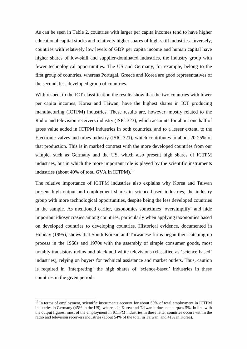
As can be seen in Table 2, countries with larger per capita incomes tend to have higher

educational capital stocks and relatively higher shares of high-skill industries. Inversely,

countries with relatively low levels of GDP per capita income and human capital have

higher shares of low-skill and supplier-dominated industries, the industry group with

fewer technological opportunities. The US and Germany, for example, belong to the

first group of countries, whereas Portugal, Greece and Korea are good representatives of

the second, less developed group of countries.

With respect to the ICT classification the results show that the two countries with lower

per capita incomes, Korea and Taiwan, have the highest shares in ICT producing

manufacturing (ICTPM) industries. These results are, however, mostly related to the

Radio and television receivers industry (ISIC 323), which accounts for about one half of

gross value added in ICTPM industries in both countries, and to a lesser extent, to the

Electronic valves and tubes industry (ISIC 321), which contributes to about 20-25% of

that production. This is in marked contrast with the more developed countries from our

sample, such as Germany and the US, which also present high shares of ICTPM

industries, but in which the more important role is played by the scientific instruments

industries (about 40% of total GVA in ICTPM).10

The relative importance of ICTPM industries also explains why Korea and Taiwan

present high output and employment shares in science-based industries, the industry

group with more technological opportunities, despite being the less developed countries

in the sample. As mentioned earlier, taxonomies sometimes ‘oversimplify’ and hide

important idiosyncrasies among countries, particularly when applying taxonomies based

on developed countries to developing countries. Historical evidence, documented in

Hobday (1995), shows that South Korean and Taiwanese firms began their catching up

process in the 1960s and 1970s with the assembly of simple consumer goods, most

notably transistors radios and black and white televisions (classified as ‘science-based’

industries), relying on buyers for technical assistance and market outlets. Thus, caution

is required in ‘interpreting’ the high shares of ‘science-based’ industries in these

countries in the given period.

10 In terms of employment, scientific instruments account for about 50% of total employment in ICTPM industries in Germany (45% in the US), whereas in Korea and Taiwan it does not surpass 5%. In line with the output figures, most of the employment in ICTPM industries in these latter countries occurs within the radio and television receivers industries (about 54% of the total in Taiwan, and 41% in Korea).

The picture is different when one looks to the ICT producing services category. In this

case, the countries which present higher shares are mostly wealthy countries, with the

exception of Ireland and, to a lesser extent, Greece.11 The same happens with respect to

non-ICT services, and information-intensive and non-market services industries, the

latter two representing categories from the innovation taxonomy. In all cases, the higher

output shares found in more developed nations reflect the more advanced nature of the

tertiarization processes in these countries, stemming from changes taking place from the

1960s onwards in trade, technology and demand factors (e.g., Feinstein, 1999; Peneder

et al., 2003; Castellacci, 2008).12

This impression is confirmed by the computation of Pearson bi-variate correlation

coefficients, considering both data on value added and employment variables (cf. Table

3). The high positive relationship between education and per capita income and,

inversely, the strong negative relationship of each of these variables and the relative

shares of low-skilled and less innovative industries is clearly apparent. All the

correlation coefficients relating education (or per capita GDP) to either the shares of

low-skill or supplier-dominated industries are negative and strongly significant. The

more odd results, namely, the negative correlation of science-based and ICT industry

shares with both education and per capita GDP reflect the specificities of the Korean

and Taiwanese economies. As indicated earlier, these countries show the highest shares

of ICT producing manufacturing activities, which are also classified as ‘science-based’,

but these industries reflect mostly assembly-line production, that requires only minor

skills of the workforce (e.g., Hobday, 1995).

Table 3

3.3. Hierarchical clustering results

Cluster analysis involves a number of different procedures that allow for the division of

a specific dataset into distinct groups, such that the degree of homogeneity is maximal if

the observations belong to the same group and minimal otherwise. In the present study,

because the dataset is relatively small, we use the hierarchical clustering approach to

classify the individual observations into clusters of maximum homogeneity.

11 Korea and Taiwan, along with Portugal, show the lowest results. 12 With regard to the employment variable, tertiarisation can also be explained by the well-known cost-disease argument developed by Baumol (Baumol, 1967, 2001).

Hierarchical clustering identifies successive clusters by using previously established

clusters. It can be either agglomerative or divisive, although the former is the most

commonly used.13 In the present case, we opted for the agglomerative approach, starting

with each case as a separate cluster and successively merging the two closest clusters

until a single, all-inclusive cluster remains.

The application of hierarchical agglomerative clustering requires the prior definition of

a criterion to determine the distance or similarity between cases. We apply the cosine

similarity criterion, although there is no clear-cut indication as to this measure’s

superiority in comparison to the others.14 It also requires the definition of the rules for

cluster formation. In the present case, we use the average linkage between groups

method, also known as UPGMA (Unweighted Pair Group Method using Arithmetic

averages). This method defines the distance between two clusters as the average

distance between all pairs of cases in the two different clusters.15 Agglomerative

clustering is applied to the standardized scores of the variables, rather than to their real

values, because they are measured on different scales (industry share variables in

percentage points, human capital in years, and per capita income in PPP current

international US dollars).

Figure 1 presents the resulting dendrogram. The first vertical lines represent the smallest

rescaled distance, which in the present case corresponds to the merging of Portugal and

Spain on the one hand, and of Sweden and the US, on the other. Subsequent vertical

lines represent merges at higher distances, until only one cluster, encompassing all

cases, is obtained.

Figure 1

Generally, a good cluster solution is defined as being the one which precedes a sudden

gap in the similarity (or distance) coefficient. In this case, the larger distance between

sequential vertical lines occurs approximately between 15 and 25, suggesting that the

best clustering solution splits the list of countries into two clusters:

13 See Everitt et al. (2001) and Aldenderfer and Blashfield (1985) for more information on hierarchical cluster analysis and on cluster analysis procedures in general. 14 Acknowledging the subjective nature of this choice, we have also considered distance measures, as well as the alternative similarity measure (the correlation of vectors). The resulting cluster solution was always the same. 15 The UPGMA method seems to be preferable in comparison to single and complete linkage rules, since it uses information regarding all pairs of distances, and not just the nearest or the farthest.

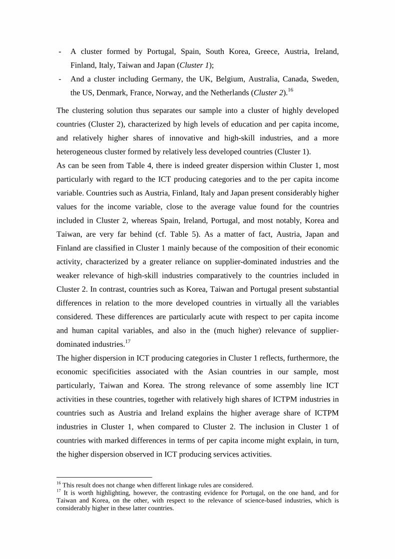
- A cluster formed by Portugal, Spain, South Korea, Greece, Austria, Ireland,

Finland, Italy, Taiwan and Japan (Cluster 1);

- And a cluster including Germany, the UK, Belgium, Australia, Canada, Sweden,

the US, Denmark, France, Norway, and the Netherlands (Cluster 2).16

The clustering solution thus separates our sample into a cluster of highly developed

countries (Cluster 2), characterized by high levels of education and per capita income,

and relatively higher shares of innovative and high-skill industries, and a more

heterogeneous cluster formed by relatively less developed countries (Cluster 1).

As can be seen from Table 4, there is indeed greater dispersion within Cluster 1, most

particularly with regard to the ICT producing categories and to the per capita income

variable. Countries such as Austria, Finland, Italy and Japan present considerably higher

values for the income variable, close to the average value found for the countries

included in Cluster 2, whereas Spain, Ireland, Portugal, and most notably, Korea and

Taiwan, are very far behind (cf. Table 5). As a matter of fact, Austria, Japan and

Finland are classified in Cluster 1 mainly because of the composition of their economic

activity, characterized by a greater reliance on supplier-dominated industries and the

weaker relevance of high-skill industries comparatively to the countries included in

Cluster 2. In contrast, countries such as Korea, Taiwan and Portugal present substantial

differences in relation to the more developed countries in virtually all the variables

considered. These differences are particularly acute with respect to per capita income

and human capital variables, and also in the (much higher) relevance of supplier-

dominated industries.17

The higher dispersion in ICT producing categories in Cluster 1 reflects, furthermore, the

economic specificities associated with the Asian countries in our sample, most

particularly, Taiwan and Korea. The strong relevance of some assembly line ICT

activities in these countries, together with relatively high shares of ICTPM industries in

countries such as Austria and Ireland explains the higher average share of ICTPM

industries in Cluster 1, when compared to Cluster 2. The inclusion in Cluster 1 of

countries with marked differences in terms of per capita income might explain, in turn,

the higher dispersion observed in ICT producing services activities.

16 This result does not change when different linkage rules are considered. 17 It is worth highlighting, however, the contrasting evidence for Portugal, on the one hand, and for Taiwan and Korea, on the other, with respect to the relevance of science-based industries, which is considerably higher in these latter countries.

Tables 4 and 5

4. Descriptive characterization of the growth and structural change processes of

‘relatively less developed countries’ countries between 1979 and 2003

Countries in Cluster 1 – ‘relatively less developed countries’, which share some similar

features in terms of economic structure in 1979, experienced very different processes of

growth and structural change from that time onwards, which gave rise to a marked

increase in their dissimilarities. Considerable differences arose with respect to GDP and

labour productivity growth, with Korea, Ireland and Taiwan experiencing very high

growth rates, well above those observed in the other countries (cf. Table 6).

Table 6

Furthermore, rapid growth experiences were intimately connected with strong structural

transformation. The computation of Nickell and Lilien indices of structural change (cf.

Table 7) reveals that the fastest growth countries – Korea, Taiwan and Ireland – were

simultaneously the countries with more rapid structural change during the period under

study.18 In contrast, slow-growing countries such as Greece or Italy experienced much

more modest changes. This is in broad agreement with the views expressed by the

authors of the new structuralist approach (e.g., Pieper, 2000; Rada and Taylor, 2006),

according to which rapid growth requires profound changes in the composition of

economic activity and external trade.

The countries with faster structural change were also the ones experiencing more

profound changes in the relative importance of the industry groups defined earlier (cf.

Table 8). Korea, Ireland and Taiwan were the countries where the decrease in the

relative share of low-skill industries was more intense. The lower importance of these

industries was compensated by a substantial increase in high-skill industries,

particularly in the cases of Ireland and Korea. Ireland, Korea and Taiwan also presented

the largest decrease in supplier-dominated industries, which, as indicated earlier, are the

industries facing lower technological opportunities. In contrast, relative shares of

18 See Lilien (1982) and Nickell (1985) for details on the computation of these indices.

specialized supplier and science-based industries – Pavitt’s top categories in

technological and innovativeness potential – increased substantially (cf. Table 8).19

Table 8

Moreover, these countries, along with Finland, presented the highest increases in ICT

producing industries, showing, at the same time, important changes in the composition

of those industries. In Taiwan and Korea, the radio and television receivers industry,

which, as indicated earlier, accounted for about one half of total value added in ICTPM

in 1979, has at the end of the period only a minor contribution (5.5% and 2.5% in gross

value added in Korea and Taiwan, respectively). In contrast, the relative importance of

electronic valves and tubes and office machinery increased substantially, representing as

a whole, more than 70% of total value added in ICTPM industries (cf. Figure 2).20 A

strong increase in the electronic valves and tubes industry is also experienced by

Ireland, rising from 3.9% to 22.5% of gross value added in 2003.

Figure 2

Given the profound changes in the structure of their economies, it is no surprise that

Korea, Ireland and Taiwan have been able to significantly modify their situation in

comparison to the more developed countries included in Cluster 2. Indeed, these

countries have dramatically reduced the gap regarding the relative importance of low-

skill and supplier-dominated industries, and converged, at the same time, in the more

technological and skill-intensive categories. In the case of Ireland, in particular, not only

was there a drastic reduction in the low-tech and low-skill industries distances, but also

a substantial increase in the already positive gap with respect to specialized supplier and

science-based industries.

Our findings seem to indicate furthermore that the influence of structural change on

economic growth depends on its association with technological change. The case of

Portugal is rather illustrative of this point. Despite showing relatively fast structural

change between 1979 and 2003, Portugal did not significantly change the composition

of its economy in terms of the industry groups considered. The country was able to

reduce the relative importance of low-skill and supplier-dominated industries and to

increase high-skill industry shares, but the rate at which this transformation took place

was relatively low. Moreover, and quite significantly, the most important change

19 In Taiwan and Korea there was however a small decline in the relative importance of science-based industries. 20 More precisely, 73.9% in Korea, and 82.4% in Taiwan.

observed during this period refers to non-market services, which increased their relative

importance in about 11 percentage points. This has probably had an influence on the

relatively poor performance of the Portuguese economy, when compared to other

countries in the sample.

Considerable changes in education also came into play during this period.21 All the

countries increased the average number of years of formal education of the working age

population, expanding human capital stocks (cf. Table 9). However, the rates at which

this increase took place differed significantly across countries. Korea shows once more

an impressive performance, along with Spain, Italy and Taiwan. Portugal, on the other

hand, presents the weakest increase in the average number of years of formal education,

and is the only country which widens the gap in comparison to the countries included in

Cluster 2.

Table 9

5. Regression analysis

The descriptive analysis developed so far suggests that an explanation for the widely

different growth patterns observed between 1979 and 2003 for countries included in the

relatively less developed cluster may reside in their differing ability to promote changes

in the economic structure towards more skilled and technology-intensive activities. In

the present section we go a step further in the examination of this assumption by

regressing actual productivity growth in the shares of some of the taxonomical

categories described earlier and their changes over time. More precisely, we estimate

the following panel regression:

ititktiktiktiktiktiktijktijkttiktiit INVINVEDUCEDUCGDPxxSCyy εµηψϕβγλδχσα +++∆++∆+++∆+++=− −−−−−−−−− 444444444444 3444444444444 2144444 344444 21variables control

,,,,,

variables change structural

,,/,,

(1)

i = country index (i = 1,…, N)

j = industry group(s) considered

t = time

µi= random disturbance related only to i

εit= error term 21 In order to get a full series of education data we extended Bassanini and Scarpetta’s (2001) estimates up to 2003 using the author’s methodology. We also applied this procedure to Korean and Taiwanese data, considering Barro and Lee’s (2001) estimates. The complete data set and some details on the calculus procedure can be found in the Annex.

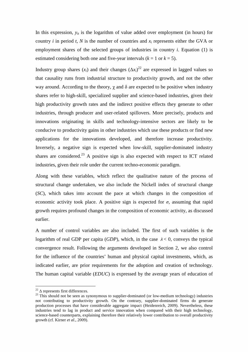
In this expression, yit is the logarithm of value added over employment (in hours) for

country i in period t, N is the number of countries and xi represents either the GVA or

employment shares of the selected groups of industries in country i. Equation (1) is

estimated considering both one and five-year intervals (k = 1 or k = 5).

Industry group shares (xi) and their changes (∆xi)22 are expressed in lagged values so

that causality runs from industrial structure to productivity growth, and not the other

way around. According to the theory, χ and δ are expected to be positive when industry

shares refer to high-skill, specialized supplier and science-based industries, given their

high productivity growth rates and the indirect positive effects they generate to other

industries, through producer and user-related spillovers. More precisely, products and

innovations originating in skills and technology-intensive sectors are likely to be

conducive to productivity gains in other industries which use these products or find new

applications for the innovations developed, and therefore increase productivity.

Inversely, a negative sign is expected when low-skill, supplier-dominated industry

shares are considered.23 A positive sign is also expected with respect to ICT related

industries, given their role under the current techno-economic paradigm.

Along with these variables, which reflect the qualitative nature of the process of

structural change undertaken, we also include the Nickell index of structural change

(SC), which takes into account the pace at which changes in the composition of

economic activity took place. A positive sign is expected for σ, assuming that rapid

growth requires profound changes in the composition of economic activity, as discussed

earlier.

A number of control variables are also included. The first of such variables is the

logarithm of real GDP per capita (GDP), which, in the case λ < 0, conveys the typical

convergence result. Following the arguments developed in Section 2, we also control

for the influence of the countries’ human and physical capital investments, which, as

indicated earlier, are prior requirements for the adoption and creation of technology.

The human capital variable (EDUC) is expressed by the average years of education of

22 ∆ represents first differences. 23 This should not be seen as synonymous to supplier-dominated (or low-medium technology) industries not contributing to productivity growth. On the contrary, supplier-dominated firms do generate production processes that have considerable aggregate impact (Heidenreich, 2009). Nevertheless, these industries tend to lag in product and service innovation when compared with their high technology, science-based counterparts, explaining therefore their relatively lower contribution to overall productivity growth (cf. Kirner et al., 2009).

the working age population, and its growth rate (∆EDUC). Physical capital

accumulation is taken into account through the inclusion of both the share of investment

in GDP (INV) and its growth rate.24 In line with our earlier discussion, the coefficients

associated to physical and human capital variables are expected to be positive. Finally,

we control for business cycle effects including time dummies (ηt).25

The estimations are calculated using the sample of countries included in Cluster 1 over

the 1980-2003 period.26 The data source for labour productivity and industry shares is

the 60-Industry GGDC Database. Data on education are taken from Bassanini and

Scarpetta (2001) and Barro and Lee (2001), and extended up to 2003 using OECD

Education at a Glance data, as indicated in the previous section. Data on gross fixed

capital formation are from the OECD Factbook 2008: Economic, Environmental and

Social Statistics, with the exception of Taiwan, whose data was taken from the

Taiwanese official government statistics.27 Finally, per capita GDP and employment

rates are taken from the World Economic Outlook Database (April 2008), developed by

the International Monetary Fund.

Tables 10-13

The results confirm our premise according to which structure influences productivity

growth, irrespective of the lag chosen or the variable used (employment or gross value

added) in the computation of industry shares (cf. Tables 10-13). In global terms, the

coefficients for the structural variables turn up with the expected signs and are, in most

cases, statistically significant.

The pace at which structural change takes place, proxied by the Nickell index (SC), is

one of the more robust explanatory variables, as it is always positive and statistically

significant. Ceteris paribus, an increase in the Nickell index in 1 percentage point

results, on average, in additional annual productivity growth of 0.27 percentage points

in 1 year lag regressions, and of about 0.13 percentage points in 5 year lag regressions.28

24 The control variables are also expressed in lagged values in order to mitigate possible endogeneity problems. 25 In previous estimations we also included the employment rate to check for country specific differences in the business cycle. Because this variable was never statistically significant and could directly influence labour productivity growth, it was excluded in the present framework. 26 One observation was lost (1979), because data on employment and investment variables was only available from 1980 onwards. Data regarding Taiwan, Korea and Japan refer to the 1980-2002 period. 27 Available on-line at http://eng.dgbas.gov.tw. 28 Cf. Table A.3 in the Annex.

Many of the variables used to reflect the direction of structural change according to the

selected technological and skill industry categories also show great robustness, although

in some cases their significance tends to decrease with the inclusion of the SC variable.

The coefficients for the skill variables, in particular, present always the expected signs

and are in most cases statistically significant.29 According to our findings, an increase in

the share of high-skill industries results in a productivity growth bonus, whereas the

opposite occurs with respect to low-skill industries.

The science-based share variable also emerges as strongly robust. The corresponding

coefficient is positive and statistically significant in all specifications, although a higher

impact over productivity growth is found when employment-based industry shares are

used instead of value added shares [cf. regressions (9) and (10) in Tables 10-13]. More

precisely, a difference of one percentage point in the science-based share gives a

difference over 0.7 percentage points in the annual productivity growth rate when

employment data are used, and about 0.3 percentage points when using value added

data.

Less robust results are found with respect to both specialized suppliers and supplier-

dominated shares, although they are in general agreement with the formulated

assumptions. The coefficients on the first variable turn out significant and with the

expected signs when employment shares are considered, but they emerge as non-

significant when value added shares are used instead. In contrast, significant results are

found with respect to supplier-dominated industries only in estimations using value

added shares. This is an interesting result, since it attests to the relevance of measuring

structural change both in terms of output and employment variables, rather than relying

on a single variable (most commonly, employment).

With regard to the influence of ICT industries over productivity growth, the results

point to a decisive role of ICT producing manufacturing (ICTPM) industries. In all the

specifications, the coefficient regarding the lagged share of this variable is positive and

strongly significant. Also noticeable is that the impact of the ICTPM share is quite

strong, particularly when employment data are considered. More precisely, assuming 1

year lags, an increase in the share of ICTPM industries by one percentage point amounts

29 Results of the estimations based on value added attest the significance of both high-skill and low-skill shares, but when employment data are used, only low-skill shares turn out significant [cf. regressions (3) - (6) in Tables 11 and 13].

to a more than one percentage point increase in the annual productivity growth rate (cf.

Table 11).

ICT producing services (ICTPS) industries, however, emerge as less relevant. The

variation in the share of these industries is only positive and significantly related to

labour productivity growth in the estimations using value added shares and 1 year lags

[cf. regressions (13) and (14) in Table 10]. Furthermore, the coefficient for the lagged

share presents always a negative sign, and is significant in the estimations considering

employment data and 1 year lags. This seemingly counter-intuitive result may reflect

the fact that two of the fastest growing countries in our sample – Korea and Taiwan –

show rather low shares in these industries during the whole period under study.

With respect to ICT-using industries, the coefficients are generally non-significant. A

significant impact over productivity growth for ICTUM and ICTUS shares is found in

the regressions of Table 11 (negative for ICTUM and positive for ICTUS), but in all

other cases there is no significant impact of ICT-using industries on productivity

growth.

Looking globally at the results on the selected industry groups variables, it can be seen

furthermore that their influence over productivity growth stems mostly from the share

variables and not from the changes in the shares. In all but two industry groups (low-

skill and ICTUS industries) there is no significant impact on productivity growth of the

changes in the industry shares. It seems therefore that the pace at which global structural

transformation takes place is important for rapid growth, as suggested by the evidence

found with respect to the SC variable, but not so much the rate of change occurring in

specific industry groups.

Regarding the control variables, the coefficients for the lagged investment rate and the

change in the education variable are never statistically significant. The education level

(EDUC) presents in most cases the expected positive sign, but is only significant in a

few regressions using 5-year lags (cf. Tables 12 and 13). The results show furthermore

that the significance of the EDUC variable tends to decrease with the inclusion of

structural change variables, which may denote that educational attainment and structural

change are to some extent correlated.30

30 It is important to note that the insignificant contribution of human capital to productivity growth appears many times in the literature, especially when panel data is used. See Temple (1999) on this matter.

The convergence or catching-up effect (proxied by the initial GDP per capita) is not

highly (statistically) relevant in specifications with 1-year lag (Tables 10-11), but turns

out negative and strongly related with productivity growth, in the case of 5-year lags

(Tables 12-13). The evidence found is globally in agreement with the (conditional)

convergence effect, that is, countries with lower initial productivity levels present, on

average, higher growth rates.

Finally, the variation in the rate of investment turns up significant in many of the

regressions estimated, particularly when 1-year lags are considered, supporting the idea

that the renewal rate of the capital stock influences growth positively. According to the

1-year lag findings, an increase in the growth rate of investment by one percentage point

amounts, on average, to an increase in annual labour productivity growth of about 0.05

percentage points.31

The positive effect of skills and technology-intensive industries on productivity growth,

controlling for the influence of other variables that might also influence growth, and

particularly its strong impact, considerably above investment in physical capital, gives

empirical support to our assumption according to which substantial benefits have

accrued to countries that successfully changed their structure towards more

technologically advanced industries. Moreover, the fact that ICTPM industries have a

strong impact on productivity growth seems to be in global agreement with the

conceptualizations of the techno-economic paradigm developed within the neo-

Schumpeterian streams of research (cf. Section 2). It is important to stress, however,

that the results lend support to the view that ICT-related industries are strategic

branches of economic activity, but only when producing industries (in the present case,

producing manufacturing industries) are considered. This underlines the fact that most

spillovers from advanced industries, and particularly ICT-producing industries are local

and national in character, and therefore that ‘buying’ is not the same as ‘producing’.

Hence, our results may be seen as reinforcing previous empirical evidence indicating

that the gains from the diffusion of new technologies are especially relevant in

economies which produce these technologies (e.g., Jaffe et al., 1993; Maurseth and

Verspagen, 1999; Jaffe and Trajtenberg, 2002).

31 Results based on 5-year lag estimations show a slightly lower estimate, of about 0.03 percentage points (cf. Tables 12 and 13).

We now explore further the relevance of ICTPM industries, considering separately the

impact of each single industry included in this group under the modelling framework

expressed in Equation (1). Tables 14 and 15 show the results.

Tables 14-15

The results are similar to our previous findings regarding the pace of global structural

change (SC) and the set of control variables (cf. Tables 14 and 15 and summary results

in Table A.3). The pace of structural transformation is again always positive and

statistically significant, and the coefficient figures are very similar. With respect to the

conditioning variables, the convergence effect is once again present, being more

important in 5-year lag regressions. The increase in the investment growth rate exerts a

positive influence on productivity growth, which is significant in most of the

regressions estimated, and particularly when considering 1-year lags. The education

level variable exhibits the correct (positive) sign but is significant only in a few

regressions. The remaining conditioning variables are never statistically significant.

The results obtained from the specific structural change variables show again that there

is no significant impact on productivity growth of the changes in the industry shares of

any of the selected industries. More importantly, the evidence found shows that the

industries included in the ICTPM group were not equally relevant in promoting labour

productivity growth.32 Although there are some differences between 1-year and 5-year

lag results, office machinery, insulated wire and scientific instruments industries emerge

as those with a decisive influence on productivity growth. The electronic valves and

tubes industry is only statistically significant when 1-year lag are considered, and

presents a less sizeable impact. The telecommunication equipment and radio and

television receivers industries, on the other hand, generally fail to be statistically

significant.33

These results are to some extent at odds with the evidence found in Carree (2003), who

found the Radio, TV and communications equipment industry as the only electronics

industry with a positive and significant impact on productivity growth. Moreover, the

average estimated impact of the specific branches of ICTPM industries in this study are,

32 As in the first set of results there is no significant impact on productivity growth of the changes in the industry shares of any of the selected industries. 33 The radio and television receivers industry is only statistically significant when considering gross value added and 5-year lags at a 10% significance level.

in general, much higher than in Carree’s work.34 Carree’s results were, however,

determined for a larger sample of OECD countries, which included developed as well as

less developed countries. Apart from differences in the estimation procedure, this result

may therefore reflect the fact that the influence of specifically-oriented structural

change in the ICTPM industries was more important in relatively less developed

economies. Perez’s contention (cf. Section 2) that relatively less developed countries

could benefit more from structural changes towards industries related to new techno-

economic paradigms in periods of transition seems in this way to get some

confirmation.

6. Conclusion

This paper explores the relationship between structural and technological change and

economic growth, taking into account a number of relatively less developed countries in

the late 1970s. According to neo-Schumpeterian notions, there are reasons to expect

technologically leading industries, and particularly those more closely related to new

technological paradigms, to have a major influence on growth. Moreover, according to

some of the views expressed (e.g., Perez, 1985), it is precisely in periods of transition

and emergence of new techno-economic paradigms that the relatively less developed

countries have greater opportunities to catch-up.

Using a simple descriptive analysis we show that rapid growth experiences during the

1979-2003 period in the countries in our sample were intimately connected with strong

structural change, measured by the computation of Nickell and Lilien indices.

Furthermore, the countries with faster structural change were also the ones experiencing

more profound increases in the relative importance of skills and innovation-intensive

industries, and the largest decreases in low-skill and supplier-dominated industries.

These results suggest that an explanation for the widely different growth patterns

observed between 1979 and 2003 for the selected countries might reside in their

differing ability to promote changes in the economic structure towards more skilled and

innovation-intensive activities.

This assumption was examined in the last part of the paper, through the estimation of

panel data regressions. According to our findings, the high-skill, science-based

34 The estimated coefficient of the only statistical significant industry in Carree’s work (from Radio, TV and communications equipment) suggests that a 1% higher share of this industry has almost 0.2% higher productivity growth per annum. Our corresponding figure is 1.2% per annum (cf. Table A3 in Annex).

industries have a positive and significant impact on productivity growth, considerably

above the influence of physical capital renewal rate and, in the case of science-based

and ICTPM industries, of the ‘global’ pace of structural change. The results thus

provide empirical support to the assumption that substantial benefits have accrued to

countries that successfully assigned larger amounts of resources to more technologically

advanced industries, namely science-based and ICT producing manufacturing

industries.

At the same time, our results lend strong support to the view that ICT-related industries

are strategic branches of economic activity, but only when producing industries are

considered. This underlines the fact that most spillovers from advanced industries, and

particularly ICT producing industries are local and national in character, and therefore

that ‘buying’ is not the same as ‘producing’. Contrarily to the conclusions presented in

other studies (e.g., Barros, 2002), we therefore argue that the implementation of

industrial policies aimed at changing the pattern of specialization towards the promotion

of leading technology sectors may pay-off. 35

References

Abramovitz, M. (1986), ‘Catching Up, Forging Ahead, and Falling Behind’. Journal of

Economic History, 46(2): 385-406.

Abramovitz, M. (1994), ‘The Origins of the Postwar Catch-Up and Convergence

Boom’, in Fagerberg, J.. B. Verspagen and N. von Tunzelmann (eds.) The

Dynamics of Technology, Trade and Growth, Aldershot: Edward Elgar, 21-52

Aldenderfer, M. S., and R. K. Blashfield (1985), Cluster Analysis. Newbury Park: Sage

Publications.

Amable, B. (1993), ‘Catch-up and convergence: a model of cumulative growth’,

International Review of Applied Economics, vol. 7 (1): 1 - 25

Amable, B. (2000), ‘International specialisation and growth’, Structural Change and

Economic Dynamics, vol. 11(1-2): 413-431

Amendola, M. and J.L. Gaffard (1998), Out of Equilibrium, Oxford: Clarendon Press.

Andersen, B., Howells, J., Hull, R., Miles, I. and Roberts, J. (eds) (2000), Knowledge

and Innovation in the New Service Economy, Cheltenham, Edward Elgar

35 Not necessarily ICT industries, since leading technologies change over time (Fagerberg, 2000).

Barro, R.J. and J.W. Lee (2001), International data on educational attainment: updates

and implications, Oxford Economic Papers, Oxford University Press.

Barros, P.P. (2002), ‘Convergence and information technologies: the experience of

Greece, Portugal and Spain’. Applied Economics Letters, 9: 675-80.

Bassanini, A. and S. Scarpetta (2001), ‘Does human capital matter for growth in OECD

countries? Evidence from pooled mean-group estimates’, OECD Economics

Department Working Paper, No. 282, OECD Publishing. doi:

10.1787/424300244276.

Baumol, W.J. (1967) ‘Macroeconomics of Unbalanced Growth: The Anatomy of Urban

Crisis’, American Economic Review, 57 (3), June: 415-426.

Baumol, W.J. (1967) ‘Macroeconomics of Unbalanced Growth: The Anatomy of Urban

Crisis’, American Economic Review, 57 (3), June: 415-426.

Baumol, W.J. (2001), ‘Paradox of the Services: Exploding Costs, Persistent Demand’,

in Ten Raa, T. and Schettkat, R. (eds.) The Growth of Service Industries: The

Paradox of Exploding Costs and Persistent Demand. Cheltenham: Edward

Elgar, pp. 3-28.

Baumol, W.J. (2002), The Free-Market Innovation Machine: Analysing the Growth

Miracle of Capitalism, Princeton, New Jersey: Princeton University Press

Baumol, W.J., Blackman, S.A.B. E Wolff, E.N. (1989), Productivity and American

Leadership: The Long View. Cambridge, MA. MIT Press,

Carree, M. (2003), Technological progress, structural change and productivity growth: a

comment, Structural Change and Economic Dynamics, vol. 14 (1): 109-115.

Clark, J., C. Freeman, and L. Soete (1981), ‘Long waves, Inventions and Innovations’,

Futures, 13, 4: 308–322.

Cornwall, J. (1976), ‘Diffusion, Convergence and Kaldor's Laws’, Economic Journal,

86: 307-314.

Cornwall, J. (1977), Modern Capitalism. Its Growth and Transformation. London,

Martin Robertson.

de la Fuente, A. and R. Doménech (2000), ‘Human capital in growth regressions: How

much difference does data quality make?’, OECD Economics Department

Working Papers No. 262.

DeLong, J.B. and L.H. Summers (1991), ‘Equipment Investment and Economic

Growth’, Quarterly Journal of Economics, 106: 2 (May): 445-502.

Denison, E.F. and W.K. Chung (1976), How Japan's Economy Grew So Fast: The

Sources of Postwar Expansion, Brookings Institution, Washington.

Dosi, G. (1982), ‘Technological Paradigms and Technological Trajectories: A

Suggested Interpretation of the Determinants and Directions of Technical

Change’, Research Policy, 11 (3), June: 147-162.

Durlauf, S., P. Jonhson (1992), ‘Local versus global convergence across national

economies’, NBER Working Paper, no. 3996.

Engelbrecht, H.-J. and Xayavong, V. (2007), “The elusive contribution of ICT to

productivity growth in New Zealand: evidence from an extended industry-level

growth accounting model”, Economics of Innovation and New Technology,

16(4): 255–275

Everitt, B. S., Leese, M. and S. Landau (2001), Cluster Analysis, Hodder Arnold, 4th

Edition

Fagerberg, J. (1994), ‘Technology and International Differences in Growth Rates’,

Journal of Economic Literature, XXXII (3): 1147-1175.

Fagerberg, J. (2000), ‘Technological progress, structural change and productivity

growth: a comparative study’, Structural Change and Economic Dynamics, 11:

393-411.

Fagerberg, J. and B. Verspagen (1999), ‘Modern Capitalism' in the 1970s and 1980s’, in

Setterfield, M. (ed.), Growth, Employment and Inflation, Macmillan, London,

pp. 113-126.

Fagerberg, J. and B. Verspagen (2002), ‘Technology-gaps, innovation-diffusion and

transformation: an evolutionary approach’, Research Policy, 31: 1291-1304.

Färe, R., S. Grosskopf and D. Margaritis (2006), ‘Productivity growth and convergence

in the European Union’, Journal of Productivity Analysis, 25: 111-141.

Feinstein, C. (1999), ‘Structural change in the developed countries during the twentieth

century’, Oxford Review of Economic Policy, 15:35-55

Franke, R. and P. Kalmbach (2005), ‘Structural change in the manufacturing sector and

its impact on business-related services: an input-output study for Germany’,

Structural Change and Economic Dynamics, 16 (2005): 467-488.

Freeman C. (1987), Technology Policy and Economic Performance, London, Pinter

Publishers.

Freeman, C. (1992), ‘Formal scientific and technical institutions in the national system

of innovation’ in Lundvall, B-E (ed.). National systems of innovation: towards a

theory of innovation and interactive learning. London: Pinter Publishers.

Freeman, C. and C. Perez (1988), ‘Structural crisis of adjustment, business cycles and

investiment behaviour’. In: Dosi, G. et alii (eds.) Technical Change and

Economic Theory. London: Pinter Publishers.

Freeman, C. and L. Soete (1997), The economics of industrial innovation. London:

Pinter.

Freeman, C., J. Clark and L. Soete (1982), Unemployment and Technical Innovation,

Pinter, London.

Grossman, G. and E. Helpman (1991), Innovation and Growth in the Global Economy,

Cambridge: MIT Press.

Gualerzi, D. (2001), Consumption and growth: Recovery and structural. Change in the

US economy. Edward Elgar, Cheltenham, UK.

Heidenreich, M. (2009), ‘Innovation patterns and location of European low- and

medium-technology industries’, Research Policy 38 (3): 483-494.

Jaffe, A.B, and M. Trajtenberg (2002), Patents, Citations and Innovations: A Window

on the Knowledge Economy, Cambridge, Mass.: MIT Press.

Jaffe, A.B, M. Trajtenberg and R. Henderson (1993), ‘Geographic localization of

knowledge spillovers as evidenced by patent citations’, Quarterly Journal of

Economics, 108: 557-798.

Kaldor, N. (1957), ‘A model of economic growth’, Economic Journal, LXVII: 591-624.

Kaldor, N. (1966), Causes of the Slow Rate of Growth in the United Kingdom,

Cambridge University Press, Cambridge.

Kaldor, N. (1970), ‘The Case for Regional Policies’, Scottish Journal of Political

Economy, XVII: 337-348.

Khan, H. (1991), ‘Measurement and determinants of socioeconomic development: A

critical conspectus’, Social Indicators Research, 24, 2: 153-175.

Kirner, E., S. Kinkel and A. Jaeger (2009) ‘Innovation paths and the innovation

performance of low-technology firms - An empirical analysis of German

industry’, Research Policy 38 (3): 447-458.

Kleinknecht, A. (1986), ‘Long waves, depressions and innovations’, De Economist,

134, 1: 84–108.

Kleinknecht, A. (1990), ‘Are there Schumpeterian waves of innovations?’, Cambridge

Journal of Economics, vol. 14, n. 1 pp. 81-92

Kox, H. and L.Rubalcaba (2007), “Business services and the changing structure of

European economic growth”, CPB Memorandum. Sector VI, Number 183. CPB

Netherlands Bureau for Economic Policy Analysis.

Kuznets, S. (1940), ‘Schumpeter’s business cycles’, American Economic Review, 30:

257–271.

Kuznets, S. (1979), ‘Growth and structural shifts’, in: Galenson, W. (ed.), Economic

Growth and Structural Change in Taiwan. The Postwar Experience of the

Republic of China, Cornell University Press, London, UK: 15-131.

Lilien, D.M. (1982), 'Sectoral shifts and cyclical unemployment', Journal of Political

Economy, vol. 90, no. 4.

Los, B. and B. Verspagen (2006), ‘The evolution of productivity gaps and specialization

patterns’, Metroeconomica, 57-4: 464-493.

Lucas, R. (1988), ‘On the Mechanics of Economic Development’, Journal of Monetary

Economics, Vol.22, pp. 3-42.

Lucas, R. E (1993), “Making a miracle”, Econometrica, 61(2), 251–272.

Lumpkin, G.T., and G.G. Dess (1996), ‘Clarifying the entrepreneurial orientation

construct and linking it to performance’, The Academy of Management Review,

21(1): 135-172.

Lundvall, B-A. (1992), National systems of innovation: towards a theory of innovation

and interactive learning. London: Pinter Publishers

Mahony, M. and M. Vechi (2009), “R&D, knowledge spillovers and company

productivity performance”, Research Policy 38: 35-44.

Maroto-Sánchez, A. and J.R. Cuadrado-Roura (2009), ‘Is growth of services an obstacle

to productivity growth? A comparative analysis’, Structural Change and

Economic Dynamics 20: 254–265.

Maurseth, P. and B. Verspagen (1999), ‘Europe: One or several systems of

innovation?’, in Fagerberg, J., Guerrieri, P., Verspagen, B. (eds.) The Economic

Challenge for Europe: Adapting to Innovation-based Growth, Elgar, Aldershot.

McDonald R.E. (2007), ‘An investigation of innovation in nonprofit organizations : The

role of organizational mission’, Nonprofit and Voluntary Sector Quarterly, vol.

36, no2: 256-281

Mensch, G., (1979), Stalemate in technology. Ballinger, Cambridge, MA.

Miles, I. and M. Tomlinson (2000), ‘Intangible Assets and Service Sectors: The

Challenges of Service Industries’, in Buiges, P, Jacquemin, A, Marchipont, J

(ed), Competitiveness and the Value of Intangible Assets , Edward Elgar.

Nelson, R and G. Wright (1992), ‘The Rise and Fall of American Technological

Leadership: The Postwar Era in Historical Perspective’ Journal of Economic

Literature, vol. 30(4): 1931-64

Nelson, R. and E. Phelps (1966), ‘Investment in humans, technological diffusion, and

economic growth’, American Economic Review: Papers and Proceedings, 51

(2): 69-75.

Nelson, R.R. (ed.) (1993), National Innovation Systems: A Comparative Analysis, New

York: Oxford University Press.

Nelson, R.R., and H. Pack (1999), ‘The Asian miracle and modern growth theory’,

Economic Journal, 109: 416-436

Nickell, S. (1985), ‘The government’s policy for jobs: an analysis’, Oxford Review of

Economic Policy, 1.

Oosterhaven, J. and A. Hoen (1998), ‘Original: Preferences, technology, trade and real

income changes in the European Union. An intercountry decomposition analysis

for 1975-1985’, The Annals of Regional Science, 32(4): 505-524.

Pasinetti, L. (1981), Structural Change and Economic Growth. A Theoretical Essay on

the Dynamics of the wealth of Nations, Cambridge University Press, Cambridge.

Pasinetti, L. (1993), Structural Economic Dynamics: A Theory of the Economic

Consequences of Human Learning, Cambridge, Cambridge University Press.

Pavitt, K. (1984), ‘Sectoral patterns of technical change: towards a taxonomy and a

theory’, Research Policy, 13: 353-369.

Peneder, M. (2003), ‘Industrial structure and aggregate growth’, Structural Change and

Economic Dynamics, 14: 427-448.

Peneder, M. (2007), ‘A sectoral taxonomy of educational intensity’, Empirica, 34: 189-

212.

Peneder, M., (2003), ‘Industrial structure and aggregate growth’, Structural Change and

Economic Dynamics, 14: 427-448.

Peneder, M., Kaniovski S., Dachs B. (2003), ‘What Follows Tertiarisation? Structural

Change and the Role of Knowledge Based Services’, The Service Industry

Journal, Vol. 23: 47-66.

Peneder, M., S. Kaniovski, B. Dachs (2003), ‘What Follows Tertiarisation? Structural

Change and the Role of Knowledge Based Services’, The Service Industry

Journal, Vol. 23: 47-66.

Perez, C. (1985), ‘Microelectronics, long waves and world structural change: New

perspectives for developing countries’, World Development, Vol.13, No. 3: 441-

463.

Petit, P. (2002), ‘Growth and Productivity in a Knowledge-Based Service Economy’, in:

Gadrey, J., Gallouj, F. (Eds.), Productivity, Innovation and Knowledge in

Services, Elgar, Cheltenham.

Petit, P. and L. Soete (2000), ‘Technical change and employment growth in services:

analytical and policy challenges’, in Technology and the future of European

employment. P. Petit and L. Soete.Aldershot, Edward Elgar.

Pieper, U. (2000), ‘Deindustrialization and the social and economic sustainability nexus

in developing countries: Cross-country evidence on productivity and

employment’, Journal of Development Studies, v. 36, no. 4, April: 66-99.

Quah, D. (1997), ‘Increasingly Weightless Economies’ in Hagemann, H. Landesmann,

M., Scazzieri, R., The Economics of Structural Change, Volume II, Critical

Writings, Aldershot: Edward Elgar.

Rada, C. and L. Taylor (2006), ‘Developing and transition economies in the late 20th

century: Diverging growth rates, economic structures, and sources of demand’,

SCEPA Working Paper 2006-1.

Robertson, P. K.Smith and N. von Tunzelmann (2009) ‘Innovation in low- and

medium-technology industries’, Research Policy 38 (3): 441-446.

Robinson, C.; L. Stokes, E. Stuivenwold and B. van Ark (2003), “Industry structure and

Taxonomies”, in Mahony, M. and Van Ark, B. (eds.), EU productivity and

competitiveness: an industry perspective. Can Europe resume the catching up

process?, Chapter 2, Enterprise Publications, European Commission.

Rosenberg, N. (1963), ‘Capital Goods, Technology, and Economic Growth’, in

Hagemann, H. Landesmann, M., Scazzieri, R., The Economics of Structural

Change, Volume I, Critical Writings, Aldershot: Edward Elgar.

Sánchez Chóliz, J. and R. Duarte (2006), ‘The effect of structural change on the self-

reliance and interdependence of aggregate sectors: the case of Spain, 1980–

1994’, Structural Change and Economic Dynamics, 17(1): 27-45.

Silva, E.G. and Teixeira, A.A.C. (2008), “Surveying Structural Change: Seminal

Contributions and a Bibliometric Account”, Structural Change and Economic

Dynamics, 19: 273-300

Temple, J. (1999), ‘A positive effect of human capital on growth’, Economics Letters

65: 131-134.

Temple, J. (2000), ‘Growth effects of education and social capital in the OECD

countries’, Economics department working papers No. 263, OECD, Paris.

Tidd, J., J. Bessant and K. Pavitt (2001), Managing innovation - integrating

technological, market and organizational change, 2nd ed., England: John Wiley

& Sons Ltd.

Timmer, M. P. (2000), The Dynamics of Asian Manufacturing – A Comparative

Perspective, 1963–1993. Edward Elgar: Cheltenham.

Timmer, M.P. and A. Szirmai (2000), ‘Productivity in Asian manufacturing: the

structural bonus hypothesis examined,’ Structural Change and Economic

Dynamics, 11: 371–392.

Timmer, M.P. and G. de Vries (2009), “Structural change and growth accelerations in

Asia and Latin America: a new sectoral data set”, Cliometrica 3: 165-190.

van Ark, B. and E. Bartelsman (2004), ‘Fostering excellence: Challenges for

productivity growth in Europe’, Background document for the Informal

Competitiveness Council Maastricht, 1st-3rd July 2004, Netherlands’ Ministry

of Economic Affairs.

Verspagen, B. (1991), ‘A New Empirical Approach to Catching up or Falling Behind’,

Structural Change and Economic Dynamics, vol. 2: 359-380

Verspagen, B. (2000), ‘Growth and Structural Change: Trends, Patterns and Policy

Options’, ECIS Working Paper, Eindhoven, The Netherlands.

Wang, L. and Szirmai, A. (2008) ‘Productivity growth and structural change in Chinese

manufacturing, 1980–2002’, Industrial and Corporate Change, 17 (4): 841–874.

Table 1: Classification of sectors according to the selected taxonomies ISIC rev.3

Industries Peneder (2002, 2007)

Tidd, Bessant and Pavitt (2001)

van Ark and Bartelsman (2004)

01 Agriculture Very low Supplier-dominated Non-ICT Other

02 Forestry Very low Supplier-dominated Non-ICT Other

05 Fishing Very low Supplier-dominated Non-ICT Other

10-14 Mining and quarrying Medium Scale-intensive Non-ICT Other

15-16 Food, drink & tobacco Low Scale-intensive Non-ICT Manufacturing

17 Textiles Very low Supplier-dominated Non-ICT Manufacturing

18 Clothing Very low Supplier-dominated ICT Using Manufacturing

19 Leather and footwear Very low Supplier-dominated Non-ICT Manufacturing

20 Wood & products of wood and cork Very low Supplier-dominated Non-ICT Manufacturing

21 Pulp, paper & paper products Medium Supplier-dominated Non-ICT Manufacturing

22 Printing & publishing Medium Supplier-dominated ICT Using Manufacturing

23 Mineral oil refining, coke & nuclear fuel Medium Scale-intensive Non-ICT Manufacturing

24 Chemicals Medium-high Science-based Non-ICT Manufacturing

25 Rubber & plastics Medium-low Specialised supplier Non-ICT Manufacturing

26 Non-metallic mineral products Low Scale-intensive Non-ICT Manufacturing

27 Basic metals Low Scale-intensive Non-ICT Manufacturing

28 Fabricated metal products Low Scale-intensive Non-ICT Manufacturing

29 Mechanical engineering Medium Specialised supplier ICT Using Manufacturing

30 Office machinery High Specialised supplier ICT Producing Manufacturing

313 Insulated wire Medium Specialised supplier ICT Producing Manufacturing

31-313 Other electrical machinery and apparatus nec Medium Science-based ICT Using Manufacturing

321 Electronic valves and tubes Medium-high Specialised supplier ICT Producing Manufacturing

322 Telecommunication equipment Medium-high Specialised supplier ICT Producing Manufacturing

323 Radio and television receivers Medium-high Science-based ICT Producing Manufacturing

331 Scientific instruments Medium-high Specialised supplier ICT Producing Manufacturing

33-331 Other instruments Medium-high Specialised supplier ICT Using Manufacturing

34 Motor vehicles Medium Scale-intensive Non-ICT Manufacturing

351 Building and repairing of ships and boats Medium-high Scale-intensive ICT Using Manufacturing

353 Aircraft and spacecraft Medium-high Scale-intensive ICT Using Manufacturing

352+359 Railroad equipment and transport equipment nec Medium-high Scale-intensive ICT Using Manufacturing

36-37 Furniture, miscellaneous manufacturing; recycling Medium-low Supplier-dominated ICT Using Manufacturing 40-41 Electricity, gas and water supply Medium Scale-intensive Non-ICT Other

45 Construction Low Supplier-dominated Non-ICT Other

50 Sale, maintenance and repair of motor vehicles and motorcycles; retail sale of automotive fuel

Low Information-intensive Non-ICT Services

51 Wholesale trade and commission trade, except of motor vehicles and motorcycles

Medium Information-intensive ICT Using Services

52 Retail trade, except of motor vehicles and motorcycles; repair of personal and household goods

Medium-low Information-intensive ICT Using Services

55 Hotels & catering Very low Supplier-dominated Non-ICT Services 60 Inland transport Medium-low Information-intensive Non-ICT Services

61 Water transport Medium-low Information-intensive Non-ICT Services 62 Air transport Medium-high Information-intensive Non-ICT Services

63 Supporting and auxiliary transport activities; activities of travel agencies

Medium Supplier-dominated Non-ICT Services

64 Communications Medium Information-intensive ICT Producing Services 65 Financial intermediation, except insurance and pension funding High Information-intensive ICT Using Services

66 Insurance and pension funding, except compulsory social security

Medium-high Information-intensive ICT Using Services

67 Activities auxiliary to financial intermediation Medium-high Information-intensive ICT Using Services 70 Real estate activities Medium Information-intensive Non-ICT Services 71 Renting of machinery and equipment Medium Information-intensive ICT Using Services 72 Computer and related activities Very high Specialised supplier ICT Producing Services 73 Research and development Very high Specialised supplier ICT Using Services

741-3 Legal, technical and advertising High Specialised supplier ICT Using Services 749 Other business activities, nec High Information-intensive Non-ICT Services 75 Public administration and defence; compulsory social security Medium-high Non-market services Non-ICT Services 80 Education Very high Non-market services Non-ICT Services 85 Health and social work Medium-high Non-market services Non-ICT Services

90-93 Other community, social and personal services Medium-high Supplier-dominated Non-ICT Services 95 Private households with employed persons Very low Supplier-dominated Non-ICT Services 99 Extra-territorial organizations and bodies Very high Non-market services Non-ICT Services

Table 2: Industry shares in total gross value added (%), average number of years of formal education of the working age population and per capita income (1979, various countries)

Skill categories Innovation categories ICT categories Education PPPpcGDP3

Agg. low1 Medium- Agg. High2 Sup.-Domin.

Scale-intensive

Spec. supplier

Science-based

Inf.-Intensive

Non-mark. serv. ICTPM ICTPS ICTUM ICTUS NICTM NICTS NICTO YEARS C. int. $

Australia 37.1 32.2 30.7 25.1 19.7 5.6 1.8 31.1 16.7 0.6 2.4 4.9 14.1 13.9 39.3 24.7 11.5 9809.80

Austria 44.5 25.0 30.6 28.2 14.8 6.1 2.4 31.9 16.6 1.4 2.4 6.2 19.8 16.3 36.1 17.9 10.3 10495.00

Belgium 33.0 24.6 42.4 18.4 17.1 11.0 4.2 29.4 19.9 1.1 4.0 5.1 24.9 16.9 32.7 15.3 9.2 9758.30

Canada 34.0 34.3 31.8 22.8 18.7 5.5 1.9 32.6 18.5 1.1 2.8 4.7 14.9 13.8 41.2 21.5 12 11119.80

Denmark 34.3 28.9 36.8 21.2 9.7 7.1 1.7 37.9 22.3 0.9 2.0 6.7 21.5 10.4 45.7 12.7 10.5 10038.20

Finland 41.2 32.0 26.8 33.4 13.2 6.3 2.0 30.0 15.1 0.8 2.5 8.7 14.3 17.7 36.3 19.7 9.5 8763.60

France 35.0 27.1 37.9 23.5 11.5 10.7 2.8 34.2 17.2 1.8 3.4 7.5 17.5 13.9 41.1 14.8 9.5 9985.80

Germany 32.8 31.7 35.5 21.0 16.6 11.4 5.3 28.7 16.9 2.1 2.8 9.9 17.7 18.4 35.4 13.7 11.2 9796.70

Greece 54.5 22.8 22.7 38.9 9.5 2.9 0.9 34.7 13.0 0.3 3.1 6.3 15.4 11.4 39.5 24 7.9 8515.30

Ireland 49.4 18.7 31.9 35.8 13.8 11.3 3.1 24.3 11.8 1.3 5.5 5.2 20.0 15.6 24.3 28.1 8.4 6612.40

Italy 45.8 24.6 29.6 29.9 13.4 9.3 3.7 31.0 12.7 1.4 2.2 9.7 19.6 18.8 32.9 15.4 7.3 8999.20

Japan 43.2 29.3 27.5 29.1 13.4 6.5 3.9 37.7 9.4 2.2 2.2 6.7 20.9 15.2 35.8 17 10.1 8901.20

Korea 57.9 19.2 22.9 41.7 12.5 4.8 4.3 27.1 9.5 2.8 1.1 4.3 16.5 17.7 24.8 32.7 6.83 2486.80

Netherlands 31.1 26.5 42.4 21.9 15 6.3 4.0 29.3 23.5 1.8 2.3 5.2 18.8 12.2 41.8 17.8 10 10696.10

Norway 34.3 35.4 30.4 19.6 21.8 4.8 2.0 34.6 17.2 0.8 2.1 6.0 16.0 11.7 40.6 22.8 10.6 12576.60

Portugal 49.8 23.1 27.1 33.4 11.7 6.1 2.2 33.8 12.8 0.8 1.5 4.1 22.5 17.3 30.9 22.8 6.9 5130.10

Spain 51.5 23.9 24.6 32.1 14.8 5.3 2.9 31.9 13.0 1.0 1.9 6.4 15.7 18.2 37.6 19.1 6.3 7287.50

Sweden 31.1 31.0 37.9 23.4 12.2 8.1 2.0 31.8 22.4 1.7 2.8 7.3 16.1 13.5 44.6 14.1 10 9953.50

Taiwan 48.6 24.3 27.2 30.3 18 6.5 5.0 29.4 10.8 3.5 1.6 8.8 17.8 24.1 25.8 18.3 6.43 3355.70

UK 31.3 33.1 35.6 21.1 18.8 9.6 3.2 30.4 16.9 1.7 2.8 9.5 16.9 14.8 37.3 16.9 10 8636.40

US 32.1 30.7 37.2 18.9 14.4 9.2 2.7 35.9 19.0 1.9 3.9 7.4 20.5 14.3 40 12.2 12.2 12255.10

Average 40.6 27.5 31.9 27.1 14.8 7.3 3 31.8 16 1.5 2.6 6.7 18.2 15.5 36.4 19.1 9.4 8817.80

Std. Dev. 8.7 4.8 5.9 6.9 3.3 2.4 1.2 3.4 4.1 0.8 1.0 1.8 2.9 3.2 6.0 5.3 1.8 2602.30

Max. 57.9 35.4 42.4 41.7 21.8 11.4 5.3 37.9 23.5 3.5 5.5 9.9 24.9 24.1 45.7 32.7 12.2 12576.60

Min. 31.1 18.7 22.7 18.4 9.5 2.9 0.9 24.3 9.4 0.3 1.1 4.1 14.1 10.4 24.3 12.2 6.3 2486.80

Source: Composition of economic activity: GGDC – 60 Industry Database; Education: Bassanini and Scarpetta (2001) and Barro and Lee (2001); Per capita income: IMF - World Economic Outlook Database (April 2008).

Notes: 1) Includes very low, low and medium-low skill industries; 2) Includes medium-high, high and very high skill industries; .3) Year of reference 1980.

Table 3: Correlation coefficients

GVA shares Employment shares

Classification Education Per capita GDP Education Per capita GDP

Very high 0.50** 0.56*** 0.65*** 0.70***

Aggregate high1 0.55*** 0.57*** 0.74*** 0.77***

Aggregate low2 -0.80*** -0.77*** -0.79*** -0.76*** Ski

lls

Very low -0.76*** -0.79*** -0.78*** -0.77***

Supplier-dominated -0.72*** -0.75*** -0.76*** -0.76***

Scale-intensive 0.34 0.24 0.31 0.32

Specialised supplier 0.19 0.15 0.52** 0.36

Science-based -0.24 -0.37 -0.17 -0.27

Information-intensive 0.31 0.44** 0.77*** 0.69***

Inno

vatio

n

Non-market services 0.63*** 0.71*** 0.62*** 0.75***

ICT Producing Manufacturing -0.21 -0.47** -0.07 -0.33

ICT Producing Services 0.31 0.33 0.63*** 0.62***

ICT Using Manufacturing 0.30 0.10 0.13 0.20

ICT Using Services -0.08 -0.02 0.73*** 0.55**

Non-ICT Manufacturing -0.56*** -0.64*** -0.57*** -0.61***

Non-ICT Services 0.63*** 0.79*** 0.74*** 0.85***

ICT

Non-ICT Other -0.37 -0.54** -0.73*** -0.72***

Correlation Education/ GDPpc 0.82*** 0.82***

Notes: 1) Includes medium-high, high and very high skill industries; 2) Includes very low, low and medium-low skill industries. N = 21;*** , ** Correlation is significant at the 0.01 and 0.05 levels, respectively (two-tailed test).

Table 4: Descriptive statistics - Clusters 1 and 2 (1979, sectoral shares computed using gross value added)

Skill categories (%) Innovation categories (%) ICT categories (%) Education PPPpcGDP3

Agg. low1 Medium- Agg. High2 Sup.-Domin.

Scale-intensive

Spec. supplier

Science-based

Inf.-Intensive

Non-mark. serv.

ICTPM ICTPS ICTUM ICTUS NICTM NICTS NICTO YEARS C. int. $

Cluster 1

Average 48.6 24.3 27.1 33.3 13.5 6.5 3.0 31.2 12.5 1.6 2.4 6.6 18.3 17.2 32.4 21.5 8.0 7054.7

Std. Dev. 5.2 4.0 3.1 4.4 2.2 2.3 1.2 3.8 2.2 1.0 1.2 1.9 2.7 3.2 5.7 5.4 1.5 2637.0

Coef. of variation

10.6 16.6 11.3 13.2 16.4 35.4 40.3 12.2 18.0 63.6 50.8 28.9 14.8 18.7 17.5 25.3 19.0 37.4

Cluster 2

Average 33.3 30.5 36.2 21.5 16.0 8.1 2.9 32.3 19.1 1.4 2.8 6.7 18.1 14.0 40.0 17.0 10.6 10420.6

Std. Dev. 1.9 3.4 4.1 2.1 3.8 2.4 1.2 3.0 2.5 0.5 0.7 1.8 3.2 2.2 3.8 4.3 1.0 1162.6

Coef. of variation

5.6 11.1 11.4 9.6 23.6 29.7 41.1 9.3 13.2 35.8 23.6 26.5 17.5 16.0 9.4 25.1 9.4 11.2

Source: Idem Table 2

Table 5: Absolute distances of countries included in Cluster 1 relative to average values of cluster 2

Skill categories (%) Innovation categories (%) ICT categories (%) Education PPPpcGDP3

Agg. low1 Medium- Agg. High2 Sup.-Domin.

Scale-intensive

Spec. supplier

Science-based

Inf.-Intensive

Non-mark. serv.

ICTPM ICTPS ICTUM ICTUS NICTM NICTS NICTO YEARS C. int. $

Austria 11.2 -5.5 -5.7 6.7 -1.1 -2.0 -0.5 -0.4 -2.6 0.0 -0.5 -0.6 1.8 2.3 -3.9 0.9 -0.3 74.4

Finland 7.9 1.5 -9.5 11.9 -2.8 -1.8 -0.9 -2.3 -4.1 -0.6 -0.4 2.0 -3.8 3.7 -3.7 2.8 -1.1 -1657.0

Greece 21.2 -7.7 -13.5 17.4 -6.5 -5.2 -1.9 2.3 -6.2 -1.1 0.2 -0.5 -2.7 -2.6 -0.4 7.0 -2.7 -1905.3

Ireland 16.2 -11.8 -4.3 14.2 -2.2 3.1 0.2 -8.0 -7.4 -0.1 2.6 -1.5 2.0 1.6 -15.7 11.1 -2.2 -3808.2

Italy 12.6 -5.9 -6.6 8.4 -2.6 1.1 0.8 -1.3 -6.4 0.0 -0.6 3.0 1.5 4.9 -7.1 -1.6 -3.3 -1421.3

Japan 9.9 -1.2 -8.8 7.5 -2.6 -1.7 1.0 5.4 -9.7 0.8 -0.7 0.0 2.8 1.2 -4.2 0.1 -0.5 -1519.3

Korea 24.6 -11.3 -13.3 20.2 -3.4 -3.3 1.4 -5.2 -9.6 1.4 -1.7 -2.4 -1.6 3.7 -15.2 15.8 -3.8 -7933.8

Portugal 16.5 -7.3 -9.2 11.9 -4.3 -2.0 -0.7 1.5 -6.3 -0.6 -1.3 -2.7 4.4 3.4 -9.1 5.9 -3.7 -5290.5

Spain 18.2 -6.6 -11.7 10.6 -1.2 -2.8 0.0 -0.4 -6.2 -0.4 -1.0 -0.3 -2.4 4.2 -2.3 2.2 -4.3 -3133.1

Taiwan 15.3 -6.2 -9.1 8.8 2.0 -1.6 2.1 -3.0 -8.4 2.1 -1.2 2.1 -0.3 10.1 -14.2 1.3 -4.2 -7064.9

Source: Idem Table 2. Notes: Absolute distance is calculated as the difference between the country’s variable value and the corresponding average value of cluster 2.

Table 6: GDP at constant prices, GDP per capita based on purchasing-power-parity and labour productivity (annual % change; 1979-2003)

GDP constant

prices GDP per capita

(PPP) Labour

productivity

Austria 2.2 4.9 2.6

Finland 2.4 5.1 3.0

Greece 2.0 4.3 1.6

Ireland 5.0 7.4 5.0

Italy 1.8 4.8 1.6

Japan 2.3 5.0 3.41

Korea 7.0 9.1 5.71

Portugal 3.0 5.8 2.7

Spain 3.0 5.5 2.0

Taiwan 6.5 8.6 6.91 Source: GDP: International Monetary Fund, World Economic Outlook Database, April 2008. Labour productivity: GGDC 60-Industry Database Notes: 1) Labour productivity is defined as value added per hour worked. 2) Reference period: 1979-2002.

Table 7: Nickell and Lilien indices of structural change (1979-2003)1

Nickell index Lilien index

Austria 0.527 0.274

Finland 0.735 0.404

Greece 0.475 0.315

Ireland 0.885 0.566

Italy 0.505 0.381

Japan 0.4632 0.3522

Korea 0.8822 0.6352

Portugal 0.601 0.477

Spain 0.472 0.346

Taiwan 0.8072 0.5742 Source: GGDC 60-Industry Database Notes: 1) Indices are calculated considering 56 sectors and sectoral proportions in value added. 2) Reference period: 1979-2002.

Table 8: Change in industry output shares between 1979 and 2003 (%)

Skill categories Innovation categories ICT categories

Agg. low1 Medium- Agg. High2 Sup.-Domin.

Scale-intensive

Spec. supplier

Science-based

Inf.-Intensive

Non-mark. serv.

ICTPM ICTPS ICTUM ICTUS NICTM NICTS NICTO

Austria -9.4 3.8 5.5 -3.9 -3.7 4.7 -0.4 4.0 -0.6 0.0 1.5 0.1 2.2 -4.0 5.6 -5.3

Finland -14.1 1.9 12.2 -11.2 -4.5 6.9 0.2 5.1 3.4 3.7 3.0 -2.4 1.1 -5.9 9.1 -8.5

Greece -9.1 2.0 7.2 -7.4 -1.1 0.2 -0.1 4.1 4.4 -0.1 0.1 -2.7 2.2 -3.8 10.4 -6.2

Ireland -21.8 -0.9 22.8 -14.5 -5.6 5.5 11.6 0.2 2.8 3.0 2.6 0.9 0.6 5.2 3.2 -15.4

Italy -12.4 3.8 8.6 -7.2 -3.2 1.8 -1.5 7.1 2.8 -0.6 1.8 -3.5 3.8 -7.0 10.5 -5.1

Japan1 -13.0 5.7 7.3 -5.6 -3.1 1.5 -1.2 7.0 1.4 0.1 0.4 -1.8 3.8 -5.8 8.5 -5.2

Korea1 -23.0 6.6 16.4 -17.5 4.6 4.8 -0.6 4.9 3.8 1.4 2.1 1.1 1.3 0.0 10.7 -16.7

Portugal -15.8 2.0 13.8 -8.5 -1.7 -1.5 -0.7 1.9 10.7 -0.2 2.3 -0.2 -2.3 -5.7 15.5 -9.4

Spain -7.5 -0.6 8.2 -1.7 -4.3 1.8 -0.7 1.6 3.4 -0.6 2.2 -2.3 2.0 -6.6 9.1 -3.8

Taiwan1 -19.2 5.9 13.3 -15.0 -5.7 4.2 -1.9 14.5 3.9 2.4 1.4 -4.4 10.4 -9.3 11.1 -11.5

Note: 1) Reference period: 1979-2002.

Table 9: Average number of years of formal education of the working age population (25-64 years) (1979-2003)

Years % change Education gap1

1979 2003 1979-2003 1979 2003 Var. (years)

Austria 10.3 12.2 18.8 -0.3 -0.1 0.2

Finland 9.5 12.5 31.3 -1.1 0.1 1.2

Greece 7.9 10.4 32.0 -2.7 -1.9 0.8

Ireland 8.4 10.9 29.7 -2.2 -1.5 0.7

Italy 7.3 10.4 42.7 -3.3 -1.9 1.4

Japan 10.1 12.7 25.8 -0.5 0.3 0.8

Korea 6.8 10.8 59.3 -3.8 -1.5 2.3

Portugal 6.9 8.0 16.6 -3.7 -4.3 -0.6

Spain 6.3 9.7 54.4 -4.3 -2.6 1.7

Taiwan 6.4 8.8 38.9 -4.2 -3.5 0.7

Notes: 1) The education gap is defined as the difference between the country’s value and the average of countries included in cluster 2.

Table 10: The effect of structural change on productivity growth (GVA, 1-period lag)

Variable Paramete

r 1 2 3 4 5 6 7 8 9 10 11 12 13 14 15 16 17 18

GDPi,t-1 λ -1.389** (-1.979)

-1.051 (-1.616)

-1.483 (-0.914)

-0.712 (-0.433)

-3.496*** (-5.099)

-2.316** (-2.382)

-2.091** (-2.251

-1.873** (-2.060)

-0.795 (-1.104)

-0.639 (-0.886)

0.507 (0.352)

-0.358 (-0.473)

-0.784 (-1.012)

-0.709 (-0.920)

-1.053 (-1.408)

-0.795 (-1.050)

-0.160 (-0.187)

-0.494 (-0.598)

EDUC i,t-1 γ 0.088 (0.391)

0.044 (0.199)

-0.260 (-0.481)

-0.454 (-0.840)

0.014 (0.080)

-0.189 (-0.677)

-0.133 (-0.431

-0.112 (-0.377)

-0.046 (-0.151)

-0.087 (-0.286)

-0.590 (-1.052)

-0.236 (-0.719)

-0.107 (-0.359)

-0.119 (-0.401)

-0.163 (-0.537)

-0.205 (-0.650)

-0.196 (-0.575)

-0.166 (-0.522)

∆EDUC i,t-1 β 0.107

(0.494) 0.101

(0.480) 0.176

(0.744) 0.126

(0.535) 0.295

(1.445) 0.196

(0.909) 0.232 (1.046

0.192 (0.878)

0.068 (0.314)

0.063 (0.292)

0.066 (0.275)

0.090 (0.411)

0.125 (0.559)

0.096 (0.433)

0.067 (0.297)

0.046 (0.209)

0.132 (0.576)

0.083 (0.371)

INV i,t-1 φ 0.005 (0.103)

-0.001 (-0.032)

-0.010 (-0.143)

-0.023 (-0.325)

0.039 (0.987)

0.021 (0.409)

0.056 (0.979

0.044 (0.797)

-0.047 (-0.957)

-0.043 (-0.896)

-0.049 (-0.670)

-0.036 (-0.718)

-0.025 (-0.515)

-0.028 (-0.574)

-0.022 (-0.440)

-0.027 (-0.547)

-0.044 (-0.866)

-0.042 (-0.856)

∆INV i,t-1 ψ 0.057** (2.265)

0.050** (2.048)

0.079*** (2.929)

0.076*** (2.839)

0.072*** (2.850)

0.060** (2.430)

0.060** (2.356

0.055** (2.174)

0.049** (1.996)

0.048** (1.968)

0.072*** (2.662)

0.053** (2.200)

0.051** (2.069)

0.049** (1.996)

0.058** (2.313)

0.054** (2.212)

0.059** (2.318)

0.056** (2.220)

SC i,t/t-1 σ 0.356*** (4.124)

0.236** (2.247)

0.233** (2.494)

0.244*** (2.655)

0.208** (2.093)

0.289*** (3.138)

0.232** (2.459)

0.253*** (2.688)

0.284*** (3.064)

Agghigh i,t-1 χ 0.257** (2.236)

0.143 (1.154)

∆Agghigh i,t-1 δ 0.116

(1.608) 0.109

(1.508)

Agg.low i,t-1 χ -0.221*** (-4.509)

-0.203** (-2.527)

Ski

lls

∆Agglow i,t-1 δ -0.195** (-2.211)

-0.089 (-0.977)

Sc.based i,t-1 χ 0.373*** (3.484)

0.264** (2.242)

∆ Sc.based i,t-1 δ 0.002

(0.070) 0.006

(0.283)

Sp.supp i,t-1 χ 0.042

(0.251) 0.065

(0.541)

∆ Sp.supp i,t-1 δ 0.000

(-0.010) -0.004

(-0.142)

Sup.domin i,t-1 χ -0.307*** (-3.130)

-0.259*** (-2.696)

Inno

vatio

n

∆Sup.domin i,t-1 δ -0.063

(-0.917) -0.051

(-0.750)

ICTPM i,t-1 χ 0.538*** (2.919)

0.400** (2.102)

0.595*** (3.216)

0.425** (2.189)

∆ICTPM i,t-1 δ -0.003

(-0.215) -0.002

(-0.141) -0.006

(-0.462) -0.005

(-0.355)

ICTPS i,t-1 χ -0.279

(-0.913) -0.178

(-0.581)

-0.210 (-0.608)

-0.022 (-0.066)

∆ICTPS i,t-1 δ 0.046* (1.838)

0.040* (1.640)

0.053** (2.102)

0.042* (1.701)

ICTUM i,t-1 χ -0.086

(-0.468) -0.118

(-0.641)

∆ICTUM i,t-1 δ -0.002

(-0.056) -0.003

(-0.084)

ICTUS i,t-1 χ 0.030

(0.273) 0.071

(0.683)

ICT

∆ICTUS i,t-1 δ -0.029

(-0.570) -0.015

(-0.291)

N. obs. 227 227 227 227 227 227 227 227 227 227 227 227 227 227 227 227 227 227

N. countries 10 10 10 10 10 10 10 10 10 10 10 10 10 10 10 10 10 10

Hausman test 8.19 8.38 13.74 14.92 10.37 7.57 6.59 7.49 3.79 4.68 20.34 5.8 7.86 9.16 6.73 7.82 5.97 7.16

R2 0.529 0.552 0.551 0.562 0.552 0.565 0.549 0.564 0.547 0.558 0.529 0.553 0.545 0.561 0.537 0.557 0.541 0.562

Legend: *** (** )[*] – statistically significant at 1%(5%)[10%]; Note: Hausman Test indicates that for all models (excluding models 3, 4 and 11) estimation with random effects (fixed effects in the case of models 3, 4 and 11).

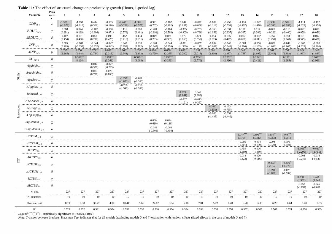
Table 11: The effect of structural change on productivity growth (Hours, 1-period lag)

Variable Paramete

r 1 2 3 4 5 6 7 8 9 10 11 12 13 14 15 16 17 18

GDPi,t-1 λ -1.389** (-1.979)

-1.051 (-1.616)

0.414 (0.306)

-0.105 (-0.110)

-2.440*** (-3.236)

-1.881*** (-2.577)

0.991 (0.707)

-0.162 (-0.182)

0.044 (0.057)

-0.072 (-0.096)

-0.889 (-1.118)

-0.450 (-0.551)

-1.116 (-1.497)

-1.042 (-1.478)

-1.588** (-2.343)

-1.362** (-1.938)

-1.114 (-1.329)

-1.177 (-1.478)

EDUC i,t-1 γ 0.088 (0.391)

0.044 (0.199)

-0.487 (-0.906)

-0.150 (-0.471)

0.116 (0.576)

0.088 (0.461)

-0.484 (-0.891)

-0.184 (-0.568)

-0.305 (-0.905)

-0.253 (-0.786)

-0.353 (-1.052)

-0.331 (-0.937)

0.127 (0.397)

0.114 (0.386)

-0.068 (-0.263)

-0.110 (-0.400)

0.022 (0.059)

0.019 (0.056)

∆EDUC i,t-1 β 0.107

(0.494) 0.101

(0.480) 0.066

(0.278) 0.093

(0.426) 0.152

(0.716) 0.134

(0.651) 0.049

(0.203) 0.081

(0.369) 0.172

(0.769) 0.121

(0.550) 0.114

(0.513) 0.105

(0.477) 0.002

(0.008) -0.002

(-0.011) 0.055

(0.259) 0.053

(0.248) 0.121

(0.549) 0.092

(0.426)

INV i,t-1 φ 0.005 (0.103)

-0.001 (-0.032)

-0.044 (-0.632)

-0.047 (-0.842)

0.040 (0.893)

0.030 (0.702)

-0.064 (-0.942)

-0.044 (-0.856)

-0.071 (-1.369)

-0.057 (-1.119)

-0.034 (-0.662)

-0.048 (-0.943)

-0.063 (-1.206)

-0.056 (-1.105)

-0.050 (-1.042)

-0.049 (-1.005)

-0.068 (-1.329)

-0.060 (-1.200)

∆INV i,t-1 ψ 0.057** (2.265)

0.050** (2.048)

0.074*** (2.734)

0.057** (2.318)

0.060** (2.344)

0.052** (2.103)

0.074** (2.720)

0.056** (2.269)

0.058** (2.290)

0.051** (2.018)

0.061** (2.408)

0.060** (2.387)

0.046* (1.788)

0.043* (1.695)

0.061** (2.443)

0.058** (2.303)

0.049** (1.967)

0.045* (1.839)

SC i,t/t-1 σ 0.356*** (4.124)

0.299*** (3.261)

0.349*** (4.063)

0.299*** (3.293)

0.265*** (2.770)

0.275*** (2.936)

0.224** (2.423)

0.159* (1.685)

0.268*** (2.966)

Agghigh i,t-1 χ 0.044

(0.321) -0.027

(-0.295)

∆Agghigh i,t-1 δ 0.073

(0.777) 0.075

(0.850)

Agg.low i,t-1 χ -0.093* (-1.852)

-0.061 (-1.266)

Ski

lls

∆Agglow i,t-1 δ -0.268

(-1.540) -0.216

(-1.266)

Sc.based i,t-1 χ 0.789* (1.841)

0.549 (1.288)

∆ Sc.based i,t-1 δ -0.037

(-1.121) -0.013

(-0.392)

Sp.supp i,t-1 χ 0.341* (1.802)

0.153 (0.735)

∆ Sp.supp i,t-1 δ -0.060

(-1.438) -0.059

(-1.442)

Sup.domin i,t-1 χ 0.060

(0.680) 0.014

(0.186)

Inno

vatio

n

∆Sup.domin i,t-1 δ -0.042

(-0.301) -0.060

(-0.450)

ICTPM i,t-1 χ 1.047*** (3.764)

0.896*** (3.382)

1.234*** (5.051)

1.076*** (3.951)

∆ICTPM i,t-1 δ -0.005

(-0.201) -0.004

(-0.159) 0.008

(0.328) 0.006

(0.250)

ICTPS i,t-1 χ -0.755

(-1.559) -0.626

(-1.380)

-1.168** (-2.200)

-0.881* (-1.755)

∆ICTPS i,t-1 δ -0.014

(-0.422) -0.020

(-0.616)

-0.008 (-0.241)

-0.018 (-0.549

ICTUM i,t-1 χ -0.393** (-2.167)

-0.336* (-1.779)

∆ICTUM i,t-1 δ -0.090* (-1.857)

-0.078 (-1.592)

ICTUS i,t-1 χ 0.250** (1.902)

0.243* (1.948

ICT

∆ICTUS i,t-1 δ -0.052

(-0.739) -0.045 (-0.651

N. obs. 227 227 227 227 227 227 227 227 227 227 227 227 227 227 227 227 227 227

N. countries 10 10 10 10 10 10 10 10 10 10 10 10 10 10 10 10 10 10

Hausman test 8.19 8.38 30.77 4.90 10.44 9.66 24.67 6.04 6.16 7.81 5.22 6.40 6.28 6.13 6.25 6.64 6.70 9.33

R2 0.529 0.552 0.531 0.554 0.532 0.555 0.530 0.554 0.534 0.553 0.535 0.558 0.557 0.567 0.567 0.574 0.550 0.565

Legend: *** (** )[*] – statistically significant at 1%(5%)[10%]; Note: T-values between brackets; Hausman Test indicates that for all models (excluding models 3 and 7) estimation with random effects (fixed effects in the case of models 3 and 7).

Table 12: The effect of structural change on productivity growth (GVA, 5-period lag)

Variable Paramete

r 1 2 3 4 5 6 7 8 9 10 11 12 13 14 15 16 17 18

GDPi,t-1 λ -19.29*** (-4.676)

-10.35** (-2.389)

-18.98*** (-3.439)

-14.54*** (-2.653)

-18.24*** (-3.370)

-15.20*** (-3.003)

-18.87*** (-2.893)

-15.03** (-2.538)

-18.53*** (-3.077)

-9.848** (-2.401)

-12.15*** (-2.601)

-9.666** (-2.145)

-10.66** (-1.789)

-8.349 (-1.555)

-12.51*** (-2.915)

-10.24*** (-2.363)

-8.223 (-1.406)

-8.347* (-1.684)

EDUC i,t-1 γ 2.268*** (2.681)

1.455 (1.569)

1.538 (1.019)

1.305 (0.949)

1.088 (0.833)

0.781 (0.639)

1.044 (0.583)

0.915 (0.581)

1.593 (1.395)

1.497 (1.292)

1.319 (0.804)

1.107 (0.756)

0.988 (0.558)

1.040 (0.724)

1.367 (1.032)

1.151 (0.937)

1.359 (0.752)

1.381 (0.966)

∆EDUC i,t-1 β -0.212

(-0.520) -0.071

(-0.175) 0.370

(0.751) 0.193

(0.411) 0.316

(0.653) 0.265

(0.586) 0.465

(0.902) 0.305

(0.641) -0.047

(-0.103) 0.060

(0.138) 0.508

(0.945) 0.242

(0.480) 0.467

(0.834) 0.242

(0.472) 0.312

(0.634) 0.158

(0.357) 0.132

(0.230) -0.109

(-0.210)

INV i,t-1 φ -0.082 (-0.350)

-0.060 (-0.249)

0.151 (0.454)

0.041 (0.130)

0.083 (0.283)

0.013 (0.045)

0.390 (0.999)

0.233 (0.663)

-0.042 (-0.152)

-0.113 (-0.411)

-0.109 (-0.305)

-0.123 (-0.378)

-0.113 (-0.313)

-0.155 (-0.473)

-0.169 (-0.554)

-0.175 (-0.609)

-0.132 (-0.352)

-0.106 (-0.317)

∆INV i,t-1 ψ 0.156** (2.571)

0.088 (1.497)

0.113 (1.633)

0.084 (1.258)

0.183*** (2.684)

0.117* (1.653)

0.105 (1.434)

0.074 (1.076)

0.097 (1.595)

0.070 (1.162)

0.135** (1.993)

0.096 (1.478)

0.128** (1.889)

0.089 (1.337)

0.109* (1.726)

0.078 (1.241)

0.127* (1.679)

0.074 (1.015)

SC i,t/t-1 σ 0.802*** (3.575)

0.504* (1.931)

0.546** (2.127)

0.590** (2.417)

0.558** (2.034)

0.606** (2.334)

0.605** (2.011)

0.536** (1.998)

0.758*** (2.892)

Agghigh i,t-1 χ 1.126*** (2.669)

0.779* (1.881)

∆Agghigh i,t-1 δ -0.883

(-0.649) -0.171

(-0.614)

Agg.low i,t-1 χ -0.686

(-1.538) -0.724* (-1.754)

Ski

lls

∆Agglow i,t-1 δ -0.374

(-1.252) -0.138

(-0.449)

Sc.based i,t-1 χ 1.999*** (3.162)

1.685*** (2.577)

∆ Sc.based i,t-1 δ -0.040

(-0.542) -0.099

(-1.338)

Sp.supp i,t-1 χ 0.949

(1.394) 0.688

(1.128)

∆ Sp.supp i,t-1 δ -0.165

(-1.578) -0.089

(-0.880)

Sup.domin i,t-1 χ -1.515** (-2.384)

-1.295** (-2.291)

Inno

vatio

n

∆Sup.domin i,t-1 δ 0.076

(0.275) -0.080 (0.313)

ICTPM i,t-1 χ 2.350** (2.071)

1.989** (1.972)

2.782*** (3.039)

2.367*** (2.671)

∆ICTPM i,t-1 δ -0.071* (-1.660)

-0.033 (-0.716)

-0.079** (-2.083)

-0.044 (-1.076)

ICTPS i,t-1 χ -1.351

(-0.521) -1.074

(-0.488)

-2.133 (-0.828)

-0.408 (-0.192)

∆ICTPS i,t-1 δ 0.002

(0.029) 0.030

(0.402)

0.055 (0.684)

0.087 (1.156)

ICTUM i,t-1 χ 0.511

(0.494) 0.372

(0.383)

∆ICTUM i,t-1 δ -0.198

(-1.625) -0.175

(-1.497)

ICTUS i,t-1 χ -0.101

(-0.153) 0.254

(0.459)

ICT

∆ICTUS i,t-1 δ 0.140

(0.598) 0.097

(0.446)

N. obs. 50 50 40 40 40 40 40 40 40 40 40 40 40 40 40 40 40 40

N. countries 10 10 10 10 10 10 10 10 10 10 10 10 10 10 10 10 10 10

Hausman test 5.87 3.82 4.98 5.23 2.95 3.05 3.78 3.68 6.04 5.93 4.03 4.22 4.06 4.13 5.51 4.46 4.98 6.05

R2 0.826 0.862 0.862 0.879 0.862 0.878 0.871 0.892 0.861 0.874 0.836 0.864 0.863 0.875 0.864 0.879 0.851 0.869

Legend: *** (** )[*] – statistically significant at 1%(5%)[10%]; T-values between brackets; Note: Hausman Test indicates for all models estimation with random effects.

Table 13: The effect of structural change on productivity growth (Hours, 5-period lag)

Variable Paramete

r 1 2 3 4 5 6 7 8 9 10 11 12 13 14 15 16 17 18

GDPi,t-1 λ -19.29*** (-4.676)

-10.35** (-2.389)

-13.36** (-2.165)

-10.57** (-2.257)

-22.70*** (-5.158)

-13.71*** (-2.798)

-14.54** (-2.480)

-11.71** (-2.151)

-7.989 (-1.546)

-6.793 (-1.517)

-14.36*** (-2.947)

-11.12** (-2.554)

-11.16** (-2.073)

-8.810* (-1.834)

-13.54** (-2.447)

-10.26** (-2.167)

-12.78** (-2.202)

-11.56** (-2.109)

EDUC i,t-1 γ 2.268*** (2.681)

1.455 (1.569)

1.025 (0.607)

1.402** (2.036)

2.038** (2.353)

1.422 (1.557)

1.329 (0.844)

0.846 (0.555)

0.848 (0.543)

1.018 (0.752)

0.811 (0.568)

0.705 (0.582)

1.853 (1.025)

1.333 (0.929)

1.283 (0.820)

1.209 (1.036)

1.446 (0.716)

0.911 (0.512)

∆EDUC i,t-1 β

-0.212 (-0.520)

-0.071 (-0.175)

0.124 (0.237)

-0.253 (-0.743)

0.030 (0.071)

0.030 (0.074)

0.219 (0.423)

0.093 (0.197)

0.212 (0.505)

0.225 (0.447)

0.012 (0.022)

-0.125 (-0.261)

-0.008 (-0.015)

-0.097 (-0.195)

0.245 (0.429)

0.026 (0.054)

0.199 (0.362)

0.086 (0.167)

INV i,t-1 φ -0.082 (-0.350)

-0.060 (-0.249)

0.054 (0.137)

-0.083 (-0.404)

0.025 (0.104)

0.015 (0.063)

-0.005 (-0.016)

-0.093 (-0.291)

-0.175 (-0.531)

-0.207 (-0.686)

0.017 (0.053)

-0.037 (-0.128)

-0.178 (-0.494)

-0.222 (-0.673)

-0.170 (-0.484)

-0.240 (-0.808)

-0.359 (-0.966)

-0.373 (-1.060)

∆INV i,t-1 ψ

0.156** (2.571)

0.088 (1.497)

0.116 (0.597)

0.037 (0.612)

0.170** (2.532)

0.104 (1.589)

0.131* (1.870)

0.087 (1.345)

0.134** (2.066)

0.099 (1.590)

0.128** (1.953)

0.085 (1.363)

0.120* (1.813)

0.094 (1.421)

0.137** (2.046)

0.104 (1.621)

0.149** (2.212)

0.121* (1.830)

SC i,t/t-1 σ 0.802*** (3.575)

0.997*** (4.494)

0.717*** (3.048)

0.707*** (2.859)

0.587** (2.230)

0.655*** (2.690)

0.571** (2.173)

0.533** (2.068)

0.621** (2.310)

Agghigh i,t-1 χ 0.390

(0.787) -0.172

(-0.823)

∆Agghigh i,t-1 δ -0.188

(-0.796) -0.274

(-1.449)

Agg.low i,t-1 χ -0.519** (-2.440)

-0.320 (-1.345)

Ski

lls

∆Agglow i,t-1 δ -0.104

(-0.257) -0.072

(-0.190)

Sc.based i,t-1 χ 5.181** (2.401)

3.933** (1.952)

∆ Sc.based i,t-1 δ -0.043

(-0.531) -0.072

(-0.942)

Sp.supp i,t-1 χ 1.807** (2.417)

1.566** (2.497)

∆ Sp.supp i,t-1 δ -0.054

(-0.513) -0.034

(-0.351)

Sup.domin i,t-1 χ -0.455

(-1.081) -0.487

(-1.226)

Inno

vatio

n

∆Sup.domin i,t-1 δ 0.206

(0.549) 0.309

(0.911)

ICTPM i,t-1 χ 3.356* (1.907)

3.062** (2.301)

3.950** (2.534)

3.416*** (2.770)

∆ICTPM i,t-1 δ 0.004

(0.054) 0.002

(0.032) 0.001

(0.015) 0.002

(0.030)

ICTPS i,t-1 χ -2.876

(-1.033) -0.946

(-0.406)

-3.687 (-1.248)

-1.286 (-0.464)

∆ICTPS i,t-1 δ 0.026

(0.270) 0.014

(0.153)

0.020 (0.204)

0.007 (0.080)

ICTUM i,t-1 χ -0.680

(-0.550) -0.360

(-0.345)

∆ICTUM i,t-1 δ -0.148

(-0.975) -0.107

(-0.774)

ICTUS i,t-1 χ 1.033

(1.249) 1.110

(1.472)

ICT

∆ICTUS i,t-1 δ -0.094

(-0.520) -0.114

(-0.656)

N. obs. 40 40 40 40 40 40 40 40 40 40 40 40 40 40 40 40 40 40

N. countries 10 10 10 10 10 10 10 10 10 10 10 10 10 10 10 10 10 10

Hausman test 5.87 3.82 3.01 15.89 5.16 4.03 3.88 3.89 2.82 5.39 3.03 2.88 3.98 2.84 2.60 2.67 4.59 5.00

R2 0.826 0.862 0.838 0.873 0.826 0.866 0.831 0.874 0.847 0.866 0.837 0.863 0.868 0.876 0.864 0.879 0.65 0.879

Legend: *** (** )[*] – statistically significant at 1%(5%)[10%]; Note: T-values between brackets; Hausman Test indicates for all models estimation with random effects.

Table 14: The effect of structural change on productivity growth – impact of ICTPM industries (1-period lag) GVA Hours

Variable

Parameter 1 2 3 4 5 6 1 2 3 4 5 6

GDPi,t-1 λ -0.808 (-1.097)

-0.585 (-0.826)

-1.571* (-1.707)

-0.250 (-0.339)

-0.092 (-0.109)

-1.804*** (-2.829)

-2.617*** (-5.168)

-1.196* (-1.746)

-1.372* (-1.735)

-0.246 (-0.335)

-0.209 (-0.254)

-2.594*** (-4.097)

EDUC i,t-1 γ -0.055 (-0.184)

0.131 (0.411)

-0.034 (-0.108)

-0.208 (-0.632)

-0.254 (-0.762)

0.133 (0.748)

0.305** (2.482)

0.277 (0.981)

0.047 (0.159)

-0.195 (-0.593)

-0.248 (-0.743)

0.208 (1.309)

∆EDUC i,t-1 β 0.161

(0.738) 0.373

(1.704) 0.164

(0.734) 0.073

(0.333) 0.077

(0.341) 0.123

(0.599) 0.198

(1.098) 0.020

(0.094) 0.070

(0.321) 0.094

(0.427) 0.105

(0.473) 0.112

(0.569)

INV i,t-1 φ -0.020 (-0.414)

-0.038 (-0.795)

-0.051 (-1.001)

-0.048 (-0.937)

-0.041 (-0.824)

0.034 (0.813)

0.019 (0.601)

-0.051 (-1.075)

-0.036 (-0.745)

-0.041 (-0.791)

-0.047 (-0.933)

0.031 (0.809)

∆INV i,t-1 ψ 0.051** (2.106)

0.040 (1.602)

0.067*** (2.643)

0.054** (2.250)

0.053** (2.199)

0.045* (1.834)

0.039* (1.645)

0.038 (1.540)

0.061** (2.454)

0.052** (2.130)

0.059** (2.387)

0.048* (1.958)

SC i,t/t-1 σ 0.284*** (3.118)

0.283*** (3.112)

0.250*** (2.590)

0.311*** (3.422)

0.285*** (3.098)

0.346*** (3.991)

0.180** (2.275)

0.206** (2.210)

0.288*** (3.173)

0.298** (3.274)

0.267*** (2.865)

0.324*** (3.862)

ISIC 30i,t-1 χ 0.888** (1.961)

3.125*** (7.669)

∆ISIC 30i,t-1 δ 0.004 (0.893)

0.009

(1.475)

ISIC 313i,t-1 χ 0.721** (2.298)

1.433*** (3.655)

∆ISIC 313i,t-1 δ -0.004

(-0.453)

-0.014 (-1.269)

ISIC 321i,t-1 χ 1.043*** (2.620)

1.696*** (3.194)

∆ISIC 321i,t-1 δ -0.003

(-0.386)

-0.003 (-0.282)

ISIC 322i,t-1 χ -0.086

(-0.281)

-0.176 (-0.199)

∆ISIC 322i,t-1 δ -0.011

(-1.414)

0.006 (0.458)

ISIC 323i,t-1 χ 0.279

(0.398)

0.222 (0.345)

∆ISIC 323i,t-1 δ -0.005

(-0.818)

-0.014 (-1.303)

ISIC 331i,t-1 χ 1.846** (1.959)

4.430*** (3.613)

ICT

PM

ind

ust

rie

s

∆ISIC 331i,t-1 δ -0.009

(-0.869)

-0.041** (-2.190)

N. obs. 227 227 227 227 227 227 227 227 227 227 227 227

N. countries 10 10 10 10 10 10 10 10 10 10 10 10

Hausman test 5.31 7.41 5.68 7.07 10.72 10.19 9.53 6.21 5.00 7.20 10.09 11.66

R2 0.557 0.555 0.561 0.56 0.555 0.553 0.565 0.561 0.560 0.553 0.557 0.570

Legend: *** (** )[*] – statistically significant at 1%(5%)[10%]; Note: T-values between brackets; Hausman test indicates for all models estimation with random effects.

Table 15: The effect of structural change on productivity growth – impact of ICTPM industries (5-period lag) GVA Hours

Variable

Parameter 1 2 3 4 5 6 1 2 3 4 5 6

GDPi,t-1 λ -10.273** (-2.038)

-7.920* (-1.895)

-11.104** (-2.277)

-7.788 (-1.614)

-4.472 (-0.924)

-13.932*** (-3.192)

-14.294*** (-2.727)

-9.309** (-2.487)

-9.244** (-1.959)

-7.565 (-1.631)

-4.993 (-1.031)

-12.104** (-2.457)

EDUC i,t-1 γ 1.303 (0.925)

2.177* (1.651)

1.489 (1.063)

0.879 (0.523)

0.554 (0.426)

1.712** (2.055)

1.799 (1.516)

2.710*** (2.762)

1.359 (0.839)

0.771 (0.487)

0.670 (0.496)

1.267 (0.987)

∆EDUC i,t-1 β 0.158

(0.320) -0.179

(-0.385) 0.156

(0.314) -0.029

(-0.053) -0.138

(-0.288) -0.162

(-0.429) -0.113

(-0.261) -0.037

(-0.095) -0.017

(-0.035) 0.063

(0.127) -0.004

(-0.008) 0.067

(0.144)

INV i,t-1 φ -0.150 (-0.481)

-0.186 (-0.638)

-0.327 (-0.943)

-0.169 (-0.433)

-0.216 (-0.729)

0.064 (0.287)

-0.200 (-0.747)

-0.271 (-1.076)

-0.250 (-0.752)

-0.064 (-0.174)

-0.196 (-0.640)

0.021 (0.071)

∆INV i,t-1 ψ 0.110* (1.732)

0.091 (1.426)

0.112* (1.728)

0.096 (1.259)

0.081 (1.311)

0.075 (1.299)

0.106* (1.823)

0.080 (1.295)

0.109* (1.667)

0.080 (1.119)

0.091 (1.462)

0.081 (1.327)

SC i,t/t-1 σ 0.669** (2.491)

0.614** (2.371)

0.680*** (2.696)

0.646** (2.201)

0.669*** (2.788)

0.691*** (2.973)

0.530** (2.157)

0.490** (2.134)

0.678** (2.551)

0.714*** (2.791)

0.700*** (2.778)

0.510* (1.905)

ISIC 30i,t-1 χ 3.632 (1.444)

9.000*** (2.642)

∆ISIC 30i,t-1 δ -0.001

(-0.086)

0.025 (1.195)

ISIC 313i,t-1 χ 3.605** (1.993)

6.494*** (3.737)

∆ISIC 313i,t-1 δ -0.026

(-0.635)

-0.036 (-0.754)

ISIC 321i,t-1 χ 2.791

(1.324)

3.941 (1.307)

∆ISIC 321i,t-1 δ -0.006

(-0.214)

-0.007 (-0.166)

ISIC 322i,t-1 χ 0.394

(0.178)

3.159 (0.550)

∆ISIC 322i,t-1 δ -0.012

(-0.294)

-0.013 (-0.347)

ISIC 323i,t-1 χ 6.157* (1.686)

5.358

(1.511)

∆ISIC 323i,t-1 δ -0.029

(-1.325)

-0.030 (-1.087)

ISIC 331i,t-1 χ 8.690* (1.872)

2.053** (1.983)

ICT

PM

ind

ust

rie

s

∆ISIC 331i,t-1 δ -0.051

(-1.490)

-0.005 (-0.101)

N. obs. 40 40 40 40 40 40 40 40 40 40 40 40

N. countries 10 10 10 10 10 10 10 10 10 10 10 10

Hausman test 4.54 6.19 5.79 3.72 6.82 5.09 2.59 5.24 5.05 3.68 5.96 2.85

R2 0.868 0.863 0.863 0.866 0.873 0,884 0.888 0.873 0.863 0.863 0.866 0.879

Legend: The dependent variable is the change in the logarithm of value added per hour; L – Level; LV - Level Variation; *** (** )[*] – statistically significant at 1%(5%)[10%]; T-values between brackets Note: Hausman Test indicates that for all models estimation with random effects.

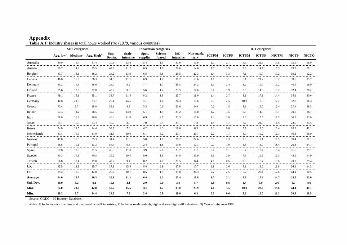
Appendix Table A.1: Industry shares in total hours worked (%) (1979, various countries)

Skill categories Innovation categories ICT categories

Agg. low1 Medium- Agg. High2 Sup.-Domin.

Scale-intensive

Spec. supplier

Science-based

Inf.-Intensive

Non-mark. serv. ICTPM ICTPS ICTUM ICTUS NICTM NICTS NICTO

Australia 49.9 18.7 31.4 30.6 13.4 5.4 1.5 33.0 16.0 1.0 2.1 6.3 22.6 13.6 35.5 18.9

Austria 59.7 14.9 25.5 42.8 11.7 6.5 1.9 22.6 14.6 1.5 1.9 7.6 14.7 15.3 29.8 29.1

Belgium 43.7 18.1 38.2 24.2 13.9 6.5 3.6 29.5 22.3 1.4 3.3 7.1 19.7 17.2 39.2 12.2

Canada 46.8 16.9 36.3 31.5 11.1 6.9 1.7 30.2 18.6 1.1 3.1 6.1 21.2 13.2 39.6 15.7

Denmark 45.2 16.8 38.0 28.7 9.2 7.7 1.7 28.5 24.2 1.1 2.4 8.2 19.7 11.2 40.6 16.9

Finland 55.6 17.3 27.0 43.2 8.6 5.6 1.4 23.5 17.6 0.7 1.9 8.8 14.8 13.2 32.4 28.2

France 49.1 15.8 35.1 33.7 11.5 8.2 1.8 25.7 19.0 1.4 2.7 8.1 17.3 14.4 35.6 20.6

Germany 44.8 21.6 33.7 28.4 14.5 10.1 4.0 24.3 18.6 2.0 2.5 10.9 17.8 17.7 32.8 16.3

Greece 72.4 9.7 18.0 55.6 9.8 3.3 0.9 20.6 9.9 0.2 1.5 8.1 12.0 12.4 27.4 38.3

Ireland 57.3 14.2 28.5 42.7 13.0 5.1 1.9 21.2 16.0 1.2 3.5 6.5 14.3 15.1 30.6 28.7

Italy 58.0 15.3 26.8 40.4 11.8 6.9 2.7 22.3 16.0 1.3 1.8 9.6 15.6 18.5 30.3 23.0

Japan 61.1 15.5 23.4 45.7 8.5 7.0 2.4 29.1 7.3 1.8 1.7 8.7 21.9 11.9 28.6 25.5

Korea 74.0 11.5 14.4 59.7 7.8 4.2 2.3 19.6 6.3 2.3 0.6 5.7 13.6 16.4 20.3 41.1

Netherlands 43.4 15.5 41.0 31.3 10.0 6.1 3.2 27.7 21.7 2.2 1.7 8.7 19.2 12.1 40.1 16.0

Norway 47.8 16.9 35.3 31.4 11.1 5.0 1.7 28.2 22.6 0.8 2.3 7.8 17.1 11.5 39.4 21.1

Portugal 66.6 10.1 23.3 54.4 9.6 2.4 1.6 19.9 12.1 0.7 1.0 5.3 13.7 18.4 26.8 34.1

Spain 67.8 10.6 21.5 46.3 11.0 3.9 2.0 23.7 13.1 0.7 1.1 6.7 15.4 15.4 31.6 29.1

Sweden 40.2 19.3 40.5 29.2 10.5 8.0 1.8 24.8 25.9 1.8 2.9 7.8 16.8 13.3 42.6 14.9

Taiwan 66.8 13.4 19.8 47.7 9.4 8.2 4.7 21.5 8.4 4.1 0.6 9.8 15.7 19.6 20.9 29.4

UK 45.5 18.8 35.7 27.3 15.5 8.8 2.9 27.8 17.7 1.9 2.6 9.1 19.2 16.8 36.1 14.3

US 39.2 18.0 42.8 25.6 10.7 8.5 1.9 29.0 24.3 2.2 2.5 7.7 20.4 12.6 44.1 10.5

Average 54.0 15.7 30.3 38.1 11.1 6.4 2.3 25.4 16.8 1.5 2.1 7.8 17.3 14.7 33.5 23.0

Std. Dev. 10.9 3.2 8.2 10.6 2.1 2.0 0.9 3.9 5.7 0.8 0.8 1.4 3.0 2.6 6.7 8.6

Max. 74.0 21.6 42.8 59.7 15.5 10.1 4.7 33.0 25.9 4.1 3.5 10.9 22.6 19.6 44.1 41.1

Min. 39.2 9.7 14.4 24.2 7.8 2.4 0.9 19.6 6.3 0.2 0.6 5.3 12.0 11.2 20.3 10.5

Source: GGDC – 60 Industry Database.

Notes: 1) Includes very low, low and medium-low skill industries; 2) Includes medium-high, high and very high skill industries; .3) Year of reference 1980.

Table A.2: Average years of education of the working age population, 1979-2003

1979 1980 1981 1982 1983 1984 1985 1986 1987 1988 1989 1990 1991 1992 1993 1994 1995 1996 1997 1998 1999 2000 2001 2002 2003

Austria 10.3 10.4 10.5 10.6 10.7 10.8 10.9 10.9 11.0 11.1 11.2 11.3 11.3 11.4 11.4 11.4 11.5 11.6 11.7 11.8 11.9 12.1 12.1 12.2 12.2

Finland 9.5 9.6 9.7 9.7 9.8 9.9 10.0 10.1 10.1 10.2 10.3 10.4 10.5 10.6 10.7 10.8 10.9 11.0 11.1 11.2 11.5 11.8 12.1 12.4 12.5

Greece 7.9 7.9 8.0 8.1 8.2 8.2 8.3 8.4 8.5 8.6 8.7 8.8 9.0 9.1 9.2 9.3 9.5 9.6 9.7 9.9 10.2 10.2 10.3 10.4 10.4

Ireland 8.4 8.5 8.6 8.7 8.8 8.9 9.0 9.0 9.1 9.2 9.3 9.4 9.5 9.6 9.7 9.8 10.0 10.1 10.2 10.3 10.5 10.6 10.8 10.9 10.9

Italy 7.3 7.3 7.4 7.5 7.6 7.7 7.8 7.9 8.0 8.1 8.2 8.4 8.5 8.6 8.8 9.0 9.2 9.4 9.6 9.8 10.0 10.1 10.2 10.4 10.4

Japan 10.1 10.2 10.3 10.4 10.5 10.6 10.7 10.8 10.9 11.0 11.1 11.2 11.4 11.5 11.6 11.7 11.9 12.0 12.1 12.3 12.3 12.4 12.5 12.7 12.7

Korea 6.8 6.8 7.0 7.3 7.5 7.8 8.0 8.3 8.5 8.7 9.0 9.3 9.4 9.6 9.7 9.9 10.1 10.2 10.2 10.3 10.4 10.5 10.5 10.6 10.8

Portugal 6.9 6.9 6.9 7.0 7.0 7.0 7.1 7.1 7.1 7.2 7.2 7.2 7.3 7.3 7.4 7.5 7.5 7.6 7.7 7.7 7.8 7.8 7.8 7.8 8.0

Spain 6.3 6.3 6.4 6.5 6.6 6.7 6.8 6.9 7.0 7.1 7.2 7.3 7.5 7.6 7.8 7.9 8.1 8.3 8.5 8.7 9.1 9.3 9.5 9.6 9.7

Taiwan 6.4 6.4 6.5 6.6 6.7 6.8 6.9 7.0 7.1 7.2 7.3 7.4 7.6 7.7 7.8 7.9 8.0 8.1 8.2 8.3 8.4 8.5 8.6 8.7 8.8

Notes: Data for the 1979-1998 period regarding all countries, except Korea and Taiwan, is from Bassanini and Scarpetta (2001). We extend Bassanini and Scarpetta’s estimates up to 2003, considering data on

educational attainment from OECD Education at a Glance (various issues), and using the cumulative years of schooling by educational level considered by the authors. Data on Korea and Taiwan between 1980 and 2000 are based on Barro and Lee (2001). We interpolate the five-year observations provided by the authors to obtain annual figures for both countries. Education estimates for Korea between 2001 and 2003 are obtained considering data on educational attainment from OECD Education at a Glance, and assuming the cumulative years of schooling used by Barro and Lee (2001). Finally, estimates regarding Taiwan for 2001, 2002 and 2003 are obtained assuming that the average years of education of the working age population during this period has grown at an annual rate similar to the one experienced in the previous quinquennium.

Table A.3: Regressions Summary (average estimates for the statistically significant coefficients) Per year estimates1

GVA(Lag 1) (Table 10)

HOURS(Lag 1) (Table 11) GVA(Lag 5)

(Table 12) HOURS(Lag 5)

(Table 13)

Y0 -2.233 (6/18) [-1.687 (2/6)]

-1.732 (5/18) [-1.945 (4/6)]

-2.887 (16/18) [-2.162 (4/6)]

-2.622 (16/18) [-2.248 (4/6)]

EDUC 0 0

[+0.305 (1/6)] +0.454(1/18) [+0.389 (2/6)]

+0.381 (3/18) [+0.542 (1/6)]

V_EDUC 0 0 0 0

INV 0 0 0 0

conditioning

variables

V_INV +0.059 [+0.054 (5/6)]

+0.056 [+0.052 (5/6)]

+0.027 (7/18) [+0.022 (2/6)]

+0.028 (9/18) [+0.022 (2/6)]

NICKELL +0.260

[+0.293] +0.277

[+0.260] +0.122

[+0.132] +0.138

[+0.121] AggHig +0.257 0 +0.191 0

V_AggHigh 0 0 0 0

Agglow -0.212 -0.093 (0 with NICK) -0.145 (incl. NICK) -0.104 (0 with NICK) skills taxonomy

V_Agglow -0.195 (0 with NICK) 0 0 0

SB +0.319 +0.789 (0 with. NICK) +0.368 +0.911

V_SB 0 0 0 0

SS 0 +0.341 (0 with NICK) 0 +0.337

V_SS 0 0 0 0

SD -0.283 0 -0.281 0

innovation taxonomy

V_SD 0 0 0 0

ICTPM +0.489 +1.063 +0.474 +0.717

V_ICPM 0 0 -0.015 (0 with NICK) 0

ICTPS 0 -1.025 0 0

V_ICTPS +0.045 0 0 0

ICTUM 0 -0.364 0 0

V_ICTUM 0 -0.090 (0 with NICK) 0 0

ICTUS 0 +0.247 0 0

ICT taxonomy

V_ICTUS 0 0 0 0

ISIC30 +0.888 +3.125 0 +1.800 Office machinery and computers

V_ ISIC30 0 0 0 0

ISIC313 +0.721 +1.433 +0.721 +1.299 Insulated wire

V_ ISIC313 0 0 0 0

ISIC321 +1.043 +1.696 0 0 Electronic valves and tubes

V_ ISIC321 0 0 0 0

ISIC322 0 0 0 0 Telecommunication equipment

V_ ISIC322 0 0 0 0

ISIC323 0 0 +1.231 0 Radio and television receivers

V_ ISIC323 0 0 0 0

ISIC331 +1.846 +4.430 +1.738 +0.411

ICTPM

Scientific instruments

V_ ISIC331 0 -0.041 0 0

Note: 1 obtained simply by dividing the average estimated coefficients in Tables 12 and 13 by five (number of periods considered in the lag). Blue figures for ICTPM specifications (Tables 14-15); 0 –statistically not significant; (x/y) means the number (x) of econometric specifications in total specification (y) estimated for which the variable achieved a statistically significant estimate.

Rescaled Distance Cluster Combine C A S E 0 5 10 15 20 25 Label Num +---------+---------+---------+---------+---------+ Portugal 16 ─┬─┐ Spain 17 ─┘ ├─┐ Korea 13 ───┘ ├───────┐ Greece 9 ─────┘ ├─────┐ Austria 2 ─────────────┘ ├─┐ Ireland 10 ───────────────────┘ ├───┐ Finland 6 ─────────────────────┘ ├─────┐ Italy 11 ─────────────┬───────────┘ ├─────────────────┐ Taiwan 19 ─────────────┘ │ │ Japan 12 ───────────────────────────────┘ │ Germany 8 ───┬─────┐ │ UK 20 ───┘ ├─────────┐ │ Belgium 3 ─────────┘ │ │ Australia 1 ─────┬─────────┐ ├─────────────────────────────┘ Canada 4 ─────┘ │ │ Sweden 18 ─┬─┐ │ │ US 21 ─┘ ├─┐ ├───┘ Denmark 5 ───┘ ├───┐ │ France 7 ─────┘ ├───┐ │ Norway 15 ─────────┘ ├─┘ Netherlands 14 ─────────────┘

Figure 1: Dendrogram using average linkage between groups and the cosine similarity measure (1979)

54

Korea

Office machinery

Electronic valves and tubes

Radio and television receivers

0%

20%

40%

60%

80%

100%

19

79

19

80

19

81

19

82

19

83

19

84

19

85

19

86

19

87

19

88

19

89

19

90

19

91

19

92

19

93

19

94

19

95

19

96

19

97

19

98

19

99

20

00

20

01

20

02

Office machinery Insulated wire Electronic valves and tubes

Telecommunication equipment Radio and television receivers Scientific instruments

Taiwan

Office machinery

Electronic valves and tubes

Radio and television receivers

0%

20%

40%

60%

80%

100%

19

79

19

80

19

81

19

82

19

83

19

84

19

85

19

86

19

87

19

88

19

89

19

90

19

91

19

92

19

93

19

94

19

95

19

96

19

97

19

98

19

99

20

00

20

01

20

02

Office machinery Insulated wire Electronic valves and tubes

Telecommunication equipment Radio and television receivers Scientific instruments

Figure 2: Evolution of the distribution of Gross Value Added in ICT Producing Manufacturing, Korea and Taiwan, 1979-2002