does spatial auto-correlation call for a revision of latest

Schröder et al. Environmental Sciences Europe 2012, 24:20http://www.enveurope.com/content/24/1/20

RESEARCH Open Access

Does spatial auto-correlation call for a revision oflatest heavy metal and nitrogen depositionmaps?Winfried Schröder1†, Roland Pesch1*†, Harry Harmens2, Hilde Fagerli3 and Ilia Ilyin4

Abstract

Background: Within the framework of the Convention on Long-range Transboundary Air Pollution atmosphericdepositions of heavy metals and nitrogen as well as critical loads/levels exceedances are mapped yearly with aspatial resolution of 50 km by 50 km. The maps rely on emission data and are calculated by use of atmosphericmodelling techniques. For validation, EMEP monitoring data collected at up to 70 sites across Europe are used. Thisspatially sparse coverage gave reason to test if the chemical and physical relations between atmosphericdepositions and their accumulation in mosses collected at up to 7000 sites throughout Europe can be quantified interms of statistical correlations which, if proven, could be used to calculate deposition maps with a higher spatialresolution. Indeed, combining EMEP maps on atmospheric depositions of cadmium, lead and nitrogen and therelated maps of their concentrations in mosses by use of a Regression Kriging approach yielded deposition mapswith a spatial resolution of 5 km by 5 km. Since spatial auto-correlation can make testing of statistical inference tooliberal, the investigation at hand was to validate the 5 km by 5 km deposition maps by analysing if spatialauto-correlation of both EMEP deposition data and moss data impacted on the significance of their statisticalcorrelation and, thus, the validity of the deposition maps. To this end, two hypotheses were tested: 1. The data ondeposition and concentrations in mosses of heavy metals and nitrogen are not spatially auto-correlatedsignificantly. 2. The correlations between the deposition and moss data lack statistical significance due to spatialautocorrelation.

Results: As already published, the regression models corroborated significant correlations between theconcentrations of heavy metals and nitrogen in atmospheric depositions on the one hand and respectiveconcentrations in mosses on the other hand. This investigation proved that atmospheric deposition andbioaccumulation data are spatially auto-correlated significantly in terms of Moran’s I values and, thus, hypothesis 1could be rejected. Accordingly, the degrees of freedom were reduced. Nevertheless, the results of the calculationsregarding the reduced degrees of freedom indicate that the statistical relations between atmospheric depositionsand bioaccumulations remained statistically significant so that hypothesis 2 could be rejected, too.

Conclusions: The positive auto-correlation in data on atmospheric deposition and bioaccumulation does not callfor a revision of the 5 km by 5 km deposition maps published in recent papers. Therefore we can conclude that theEuropean moss monitoring yields data that support the validation of modelling and mapping of atmosphericdepositions of heavy metals and nitrogen at a high spatial resolution compared to the 50 km x 50 km EMEP maps.

Keywords: Biomonitoring, Concentrations of Cd, Pb and N in mosses, Atmospheric depositions of Cd, Pb and N,EMEP deposition network and modelling, ICP Vegetation

* Correspondence: [email protected]†Equal contributors1Chair of Landscape Ecology, University of Vechta, P.O.B. 155349364, Vechta,GermanyFull list of author information is available at the end of the article

© 2012 Schröder et al.; licensee Springer. This iAttribution License (http://creativecommons.orin any medium, provided the original work is p

s an Open Access article distributed under the terms of the Creative Commonsg/licenses/by/2.0), which permits unrestricted use, distribution, and reproductionroperly cited.

mailto:[email protected]

http://creativecommons.org/licenses/by/2.0

Schröder et al. Environmental Sciences Europe 2012, 24:20 of 8http://www.enveurope.com/content/24/1/20

BackgroundMeasurements of atmospheric depositions are needed as abasis to evaluate environmental quality. To this end,deposition data are, amongst others, used to calculateexceedance maps for critical loads. Critical loads aredefined as quantitative estimates of an exposure to one ormore pollutants below which significant harmful effects onspecified ecosystem functions are not expected to occuraccording to present knowledge [1]. In Europe, the controlof heavy metals and reactive nitrogen emissions to air isregulated under several directives of the European Unionand protocols of the Long-range Transboundary Air Pollu-tion (LRTAP) Convention. Under the LRTAP Convention,the European Monitoring and Evaluation Programme(EMEP) collects emission data from European countries inorder to model atmospheric transport and depositions ofair pollutants. Amongst others, depositions of cadmium(Cd), lead (Pb) and nitrogen (N) are calculated using

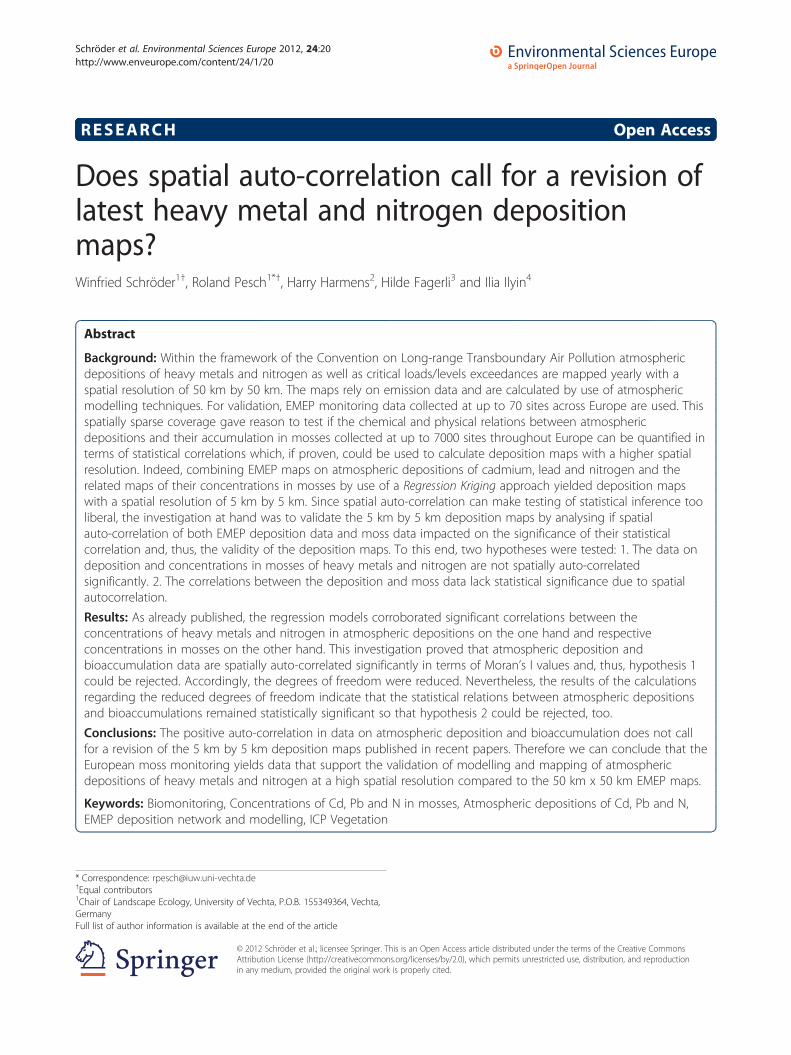
Figure 1 Moss sampling sites 2005 and EMEP raster across Europe.

chemical transport models yielding deposition maps with agrid size of 50 km by 50 km. The modelling results are vali-dated by use of deposition data collected at EMEP moni-toring sites. However, the number of EMEP measurementstations is rather limited across Europe and EMEP stationsare generally under-represented in Southern and EasternEurope. In 2005, 53 EMEP stations measured the concen-tration of nitrogen compounds in precipitation and wetdeposition, whereas up to 41 stations reported air concen-trations of nitrogen compounds [2]. In case of heavy metals,the number of EMEP measurement stations accounts forup to 70 throughout Europe [3].For ecosystem-specific evaluations of exposure in terms

of atmospheric depositions or critical loads informationwith high spatial resolution is crucial [4-10]. To enhancethe spatial resolution of the deposition maps data on phe-nomena that are physically and statistically related withdepositions and collected at higher spatial density could


be utilised. Once substances emitted to air have beendeposited, they can accumulate in plant biomass, as forinstance in mosses. The European moss biomonitoringnetwork encompassing up to 7000 sites was establishedin 1990 and has been repeated every five years sincethen [3]. Carpet-forming, ectohydric mosses obtainmost trace elements and nutrients directly from precipi-tation, occult deposition and dry deposition. Therefore,the moss technique has been shown to provide a comple-mentary, time-integrated measure of element depositionfrom the atmosphere to terrestrial systems quantifying thepotential availability of potentially harmful substances suchas heavy metals [3] or nutrients such as nitrogen [2]. Withthe moss technique a much higher sampling density can beachieved than with conventional deposition analysis. Thenational moss surveys across Europe are coordinated bythe ICP Vegetation and follow recommendations regardingsampling, preparation and chemical analyses of the mossesput down in an experimental protocol. Figure 1 shows thedistribution of moss species sampled in the 2005 survey to-gether with the EMEP 50 km x 50 km raster.The European moss monitoring produces datasets at

high spatial resolution which was used to evaluate theperformance of the EMEP model [11] and to calculatedeposition maps with a spatial resolution of 5 km by 5 kmthrough modelling the statistical relations between atmos-pheric deposition and bioaccumulation of of Cd, Pb and Nby use of Regression Kriging [12,13]. The correspondingmethodology and results can be summarised as follows:The EMEP deposition maps were intersected within a GISwith Kriging maps on N, Cd and Pb accumulations inmosses. The maps were calculated by Ordinary Kriging onbasis of the variograms presented in the ‘Results’ sectionof this paper. Next medians were calculated for all mossestimations within each EMEP grid cell. Both moss dataand corresponding modelled deposition values were ln-transformed and their relationship investigated andmodelled by linear regression analysis. The regressionmodels corroborate that the Cd concentration in mossesis correlated with the EMEP modelled total Cd depositionacross Europe (regression coefficient according to Pearson,rp = 0.67; regression coefficient according to Spearman,rs = 0.69). The coefficient of determination is R2 = 0.44.The same is true for Pb with rp = 0.76 and rs = 0.77 andR2= 0.58 [13]. The regression analysis of the estimated Nconcentrations in mosses and the modelled EMEPdepositions, too, resulted in clear linear regression pat-terns with coefficients of determination of R2 = 0.62 andPearson correlations of rp = 0.79 and Spearman correla-tions of rs = 0.70, respectively [12]. The regression equa-tions were applied on the moss kriging estimates of theelement concentration in mosses. The respective residualswere projected onto the centres of the EMEP grid cellsand were mapped using variogram analysis and ordinary

kriging. Finally, the residual and the regression map weresummed up to the map of total N, Cd, and Pb depositionin terrestrial ecosystems throughout Europe. This wasdone for a 5 km by 5 km raster which was chose due tothe results of nearest neighbourhood statistics: All nearestneighbour distances of all moss sites were calculated inArcGIS 10.0 and summarised in terms of quantilestatistics. The 10th quantile was chosen in order to adjustthe interpolation raster to the high density of the mossmonitoring net approximating ca. 5000 m (exact value:5468.5 m).By application of this environmental mapping method-

ology the EMEP maps could be improved in both spatialresolution and, by adding more empirical data, in termsof validation aspects. Due to the use of moss data themaps furthermore depict direct impacts of atmosphericpollution to terrestrial ecosystem functions since the up-take of pollutants by plants can be seen as the first steptowards an effect.Auto-correlation is a widespread phenomenon in envir-

onmental systems [14,15]. In statistics, the auto-correlationof a random process is defined as the similarity of, or cor-relation between, values of a process at neighbouring pointsin time or space. Auto-correlation describes the similaritybetween observations as a function of the separation oftime and space intervals between them. Positive auto-correlation means that the individual observations containinformation which is part of other, timely or spatial neigh-bouring, observations. Subsequently, the effective samplesize will be lower than the number of realized observations.Negative auto-correlation can have the opposite effect, thus,making the effective sample larger than the realized sample[16]. Therefore, autocorrelation can have several implica-tions for calculating statistics of measurement data in termsof statistical inference testing [17,18]. Initially, investigationsof statistical implications of auto-correlation concentratedmainly on time series analysis and were followed by investi-gations of the impacts of spatial auto-correlation on infer-ence testing methods. For instance, it could be shown, thatpositive spatial auto-correlation enhances type I errors, sothat parametric statistics such as Pearson correlation coeffi-cients, are declared significant when they should not be[19]. These findings gave reason for the investigation athand aiming at validating recently published depositionmaps which were derived by a Regression Kriging approach[12,13].

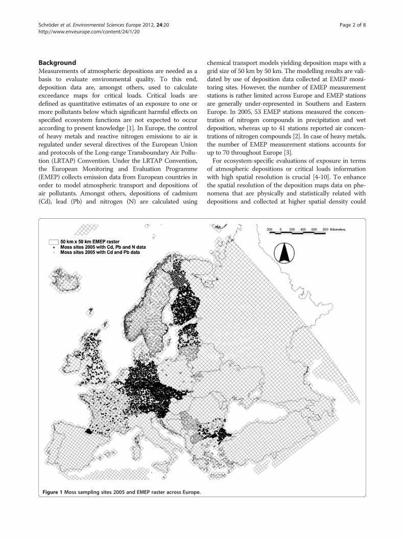
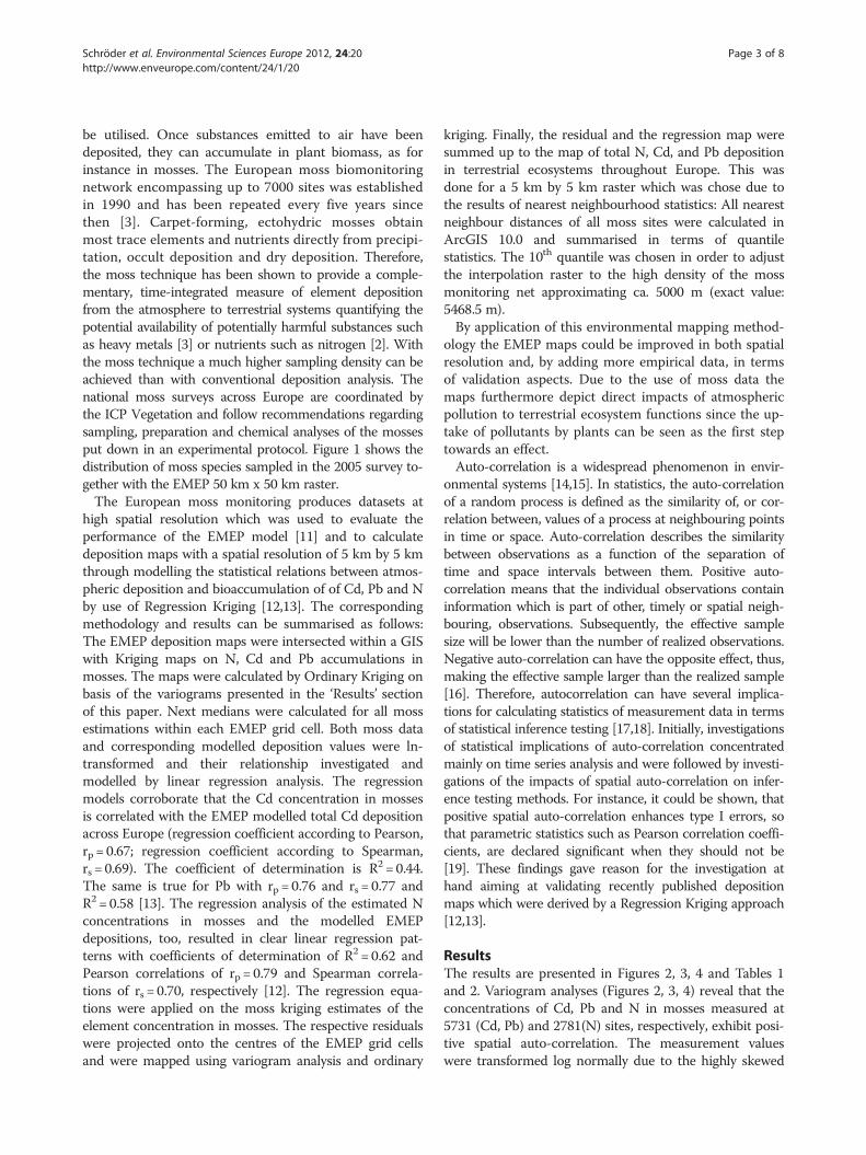
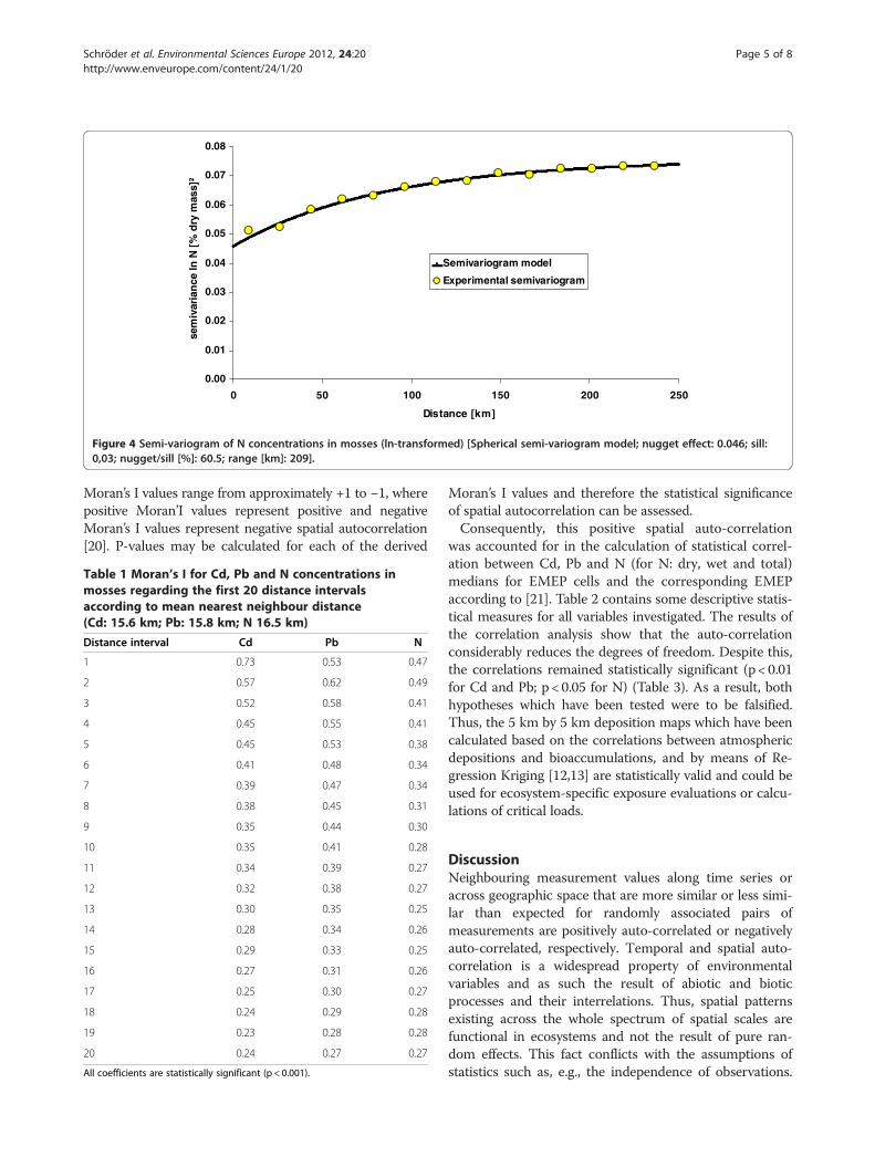
ResultsThe results are presented in Figures 2, 3, 4 and Tables 1and 2. Variogram analyses (Figures 2, 3, 4) reveal that theconcentrations of Cd, Pb and N in mosses measured at5731 (Cd, Pb) and 2781(N) sites, respectively, exhibit posi-tive spatial auto-correlation. The measurement valueswere transformed log normally due to the highly skewed

0.00

0.05

0.10

0.15

0.20

0.25

0 20 40 60 80 100 120

Distance [km]

Sem

ivar

ian

ce ln

Cd

[µg

/g]²

Semivariogram model

Experimental semivariogram

Figure 2 Semi-variogram of Cd concentrations in mosses (ln-transformed) [Exponential semi-variogram model; nugget effect: 0.13; sill:0.09; nugget/sill [%]: 59; range [km]: 59.3].


data distributions of the elements investigated (SkewnessCd=8.1; skewness Pb= 11; skewness N=1). With vario-gram analysis experimental semi-variances are calculatedin terms of half of the average squared differences of allpairs of measurement values within each distance interval.The mean nearest neighbour distances were chosen as astarting point for the distance intervals resulting in15.6 km for Cd, 15.8 km for Pb and 16.5 km for N. Thewidth of the variogram window was set so that both theincrease and the flattening of the semi-variance valueswith the separation distance could be clearly observed.Then, semi-variogram models were fitted to the experi-mental semi-variograms by a least squared regressionline. The variogram model can be described by threeparameters: range, sill and nugget-effect. The range

0.00

0.05

0.10

0.15

0.20

0.25

0.30

0.35

0 50 100

Dista

Sem

ivar

ian

ce ln

Pb

[µg

/g]²

S

E

Figure 3 Semi-variogram of Pb concentrations in mosses (ln-transform0.12; nugget/sill [%]: 61.2; range [km]: 255].

equals the maximum separation distance for which adistinct increase of semi-variogram values, and there-fore spatial autocorrelation, can be observed. The sillcorresponds to the semi-variance assigned to the range.High spatial variability within the first distance interval canbe caused by measurement errors and other confoundingfactors resulting in nugget-effects. Accordingly, the vario-gram model will tend to cut the ordinate of the variogramplot above the origin. Even though such a high nugget ef-fect can be observed for Cd, Pb and N a distinct increaseof experimental semi-variances with separation distanceproves that spatial autocorrelation exists in all three cases.Table 1 corroborates by means of calculated Moran’s I

values for the same distance intervals that this positivespatial auto-correlation is also statistically significant.

150 200 250

nce [km]

emivariogram model

xperimental semivariogram

ed) [Spherical semi-variogram model; nugget effect: 0.19; sill:

0.00

0.01

0.02

0.03

0.04

0.05

0.06

0.07

0.08

0 50 100 150 200 250

Distance [km]

sem

ivar

ian

ce ln

N [

% d

ry m

ass]

²

Semivariogram model

Experimental semivariogram

Figure 4 Semi-variogram of N concentrations in mosses (ln-transformed) [Spherical semi-variogram model; nugget effect: 0.046; sill:0,03; nugget/sill [%]: 60.5; range [km]: 209].


Moran’s I values range from approximately +1 to −1, wherepositive Moran’I values represent positive and negativeMoran’s I values represent negative spatial autocorrelation[20]. P-values may be calculated for each of the derived

Table 1 Moran’s I for Cd, Pb and N concentrations inmosses regarding the first 20 distance intervalsaccording to mean nearest neighbour distance(Cd: 15.6 km; Pb: 15.8 km; N 16.5 km)

Distance interval Cd Pb N

1 0.73 0.53 0.47

2 0.57 0.62 0.49

3 0.52 0.58 0.41

4 0.45 0.55 0.41

5 0.45 0.53 0.38

6 0.41 0.48 0.34

7 0.39 0.47 0.34

8 0.38 0.45 0.31

9 0.35 0.44 0.30

10 0.35 0.41 0.28

11 0.34 0.39 0.27

12 0.32 0.38 0.27

13 0.30 0.35 0.25

14 0.28 0.34 0.26

15 0.29 0.33 0.25

16 0.27 0.31 0.26

17 0.25 0.30 0.27

18 0.24 0.29 0.28

19 0.23 0.28 0.28

20 0.24 0.27 0.27

All coefficients are statistically significant (p < 0.001).

Moran’s I values and therefore the statistical significanceof spatial autocorrelation can be assessed.Consequently, this positive spatial auto-correlation

was accounted for in the calculation of statistical correl-ation between Cd, Pb and N (for N: dry, wet and total)medians for EMEP cells and the corresponding EMEPaccording to [21]. Table 2 contains some descriptive statis-tical measures for all variables investigated. The results ofthe correlation analysis show that the auto-correlationconsiderably reduces the degrees of freedom. Despite this,the correlations remained statistically significant (p < 0.01for Cd and Pb; p < 0.05 for N) (Table 3). As a result, bothhypotheses which have been tested were to be falsified.Thus, the 5 km by 5 km deposition maps which have beencalculated based on the correlations between atmosphericdepositions and bioaccumulations, and by means of Re-gression Kriging [12,13] are statistically valid and could beused for ecosystem-specific exposure evaluations or calcu-lations of critical loads.

DiscussionNeighbouring measurement values along time series oracross geographic space that are more similar or less simi-lar than expected for randomly associated pairs ofmeasurements are positively auto-correlated or negativelyauto-correlated, respectively. Temporal and spatial auto-correlation is a widespread property of environmentalvariables and as such the result of abiotic and bioticprocesses and their interrelations. Thus, spatial patternsexisting across the whole spectrum of spatial scales arefunctional in ecosystems and not the result of pure ran-dom effects. This fact conflicts with the assumptions ofstatistics such as, e.g., the independence of observations.

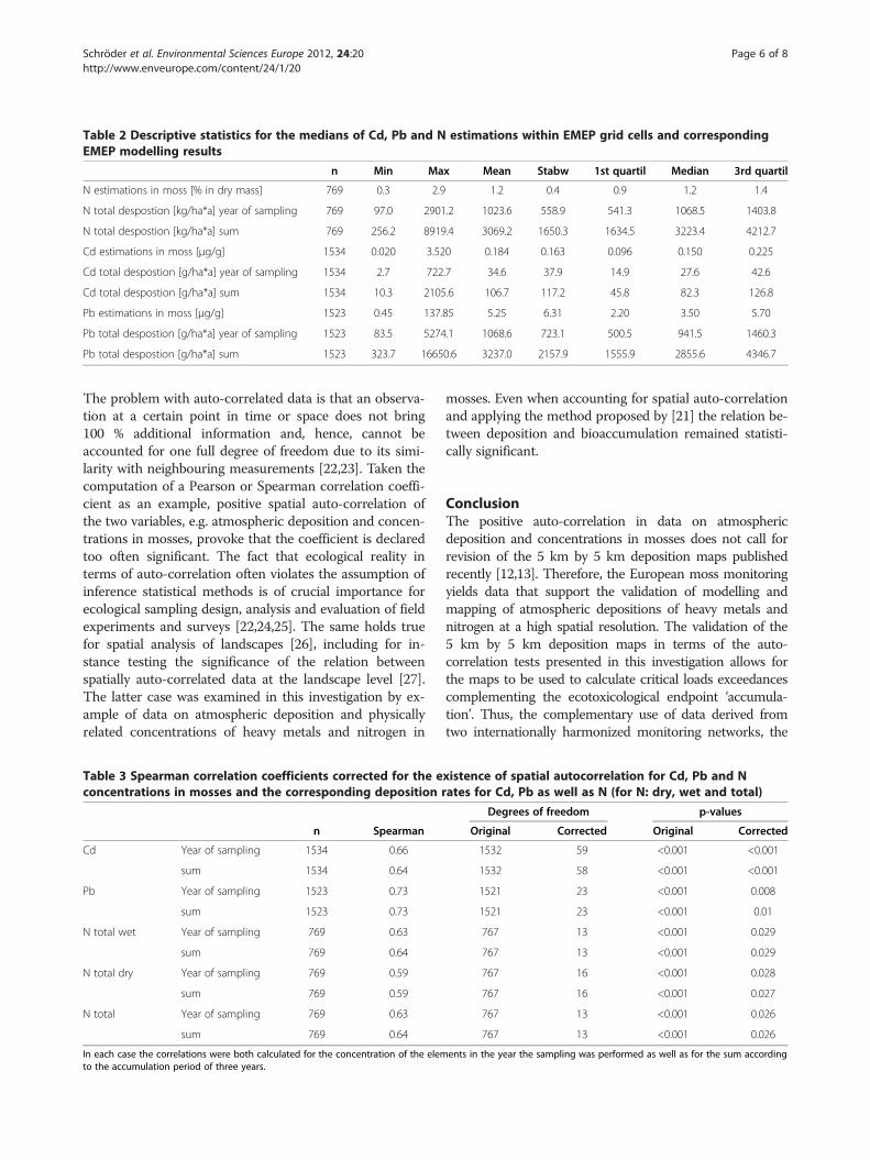
Table 2 Descriptive statistics for the medians of Cd, Pb and N estimations within EMEP grid cells and correspondingEMEP modelling results

n Min Max Mean Stabw 1st quartil Median 3rd quartil

N estimations in moss [% in dry mass] 769 0.3 2.9 1.2 0.4 0.9 1.2 1.4

N total despostion [kg/ha*a] year of sampling 769 97.0 2901.2 1023.6 558.9 541.3 1068.5 1403.8

N total despostion [kg/ha*a] sum 769 256.2 8919.4 3069.2 1650.3 1634.5 3223.4 4212.7

Cd estimations in moss [μg/g] 1534 0.020 3.520 0.184 0.163 0.096 0.150 0.225

Cd total despostion [g/ha*a] year of sampling 1534 2.7 722.7 34.6 37.9 14.9 27.6 42.6

Cd total despostion [g/ha*a] sum 1534 10.3 2105.6 106.7 117.2 45.8 82.3 126.8

Pb estimations in moss [μg/g] 1523 0.45 137.85 5.25 6.31 2.20 3.50 5.70

Pb total despostion [g/ha*a] year of sampling 1523 83.5 5274.1 1068.6 723.1 500.5 941.5 1460.3

Pb total despostion [g/ha*a] sum 1523 323.7 16650.6 3237.0 2157.9 1555.9 2855.6 4346.7


The problem with auto-correlated data is that an observa-tion at a certain point in time or space does not bring100 % additional information and, hence, cannot beaccounted for one full degree of freedom due to its simi-larity with neighbouring measurements [22,23]. Taken thecomputation of a Pearson or Spearman correlation coeffi-cient as an example, positive spatial auto-correlation ofthe two variables, e.g. atmospheric deposition and concen-trations in mosses, provoke that the coefficient is declaredtoo often significant. The fact that ecological reality interms of auto-correlation often violates the assumption ofinference statistical methods is of crucial importance forecological sampling design, analysis and evaluation of fieldexperiments and surveys [22,24,25]. The same holds truefor spatial analysis of landscapes [26], including for in-stance testing the significance of the relation betweenspatially auto-correlated data at the landscape level [27].The latter case was examined in this investigation by ex-ample of data on atmospheric deposition and physicallyrelated concentrations of heavy metals and nitrogen in

Table 3 Spearman correlation coefficients corrected for the econcentrations in mosses and the corresponding deposition r

n Spearman

Cd Year of sampling 1534 0.66

sum 1534 0.64

Pb Year of sampling 1523 0.73

sum 1523 0.73

N total wet Year of sampling 769 0.63

sum 769 0.64

N total dry Year of sampling 769 0.59

sum 769 0.59

N total Year of sampling 769 0.63

sum 769 0.64

In each case the correlations were both calculated for the concentration of the elemto the accumulation period of three years.

mosses. Even when accounting for spatial auto-correlationand applying the method proposed by [21] the relation be-tween deposition and bioaccumulation remained statisti-cally significant.

ConclusionThe positive auto-correlation in data on atmosphericdeposition and concentrations in mosses does not call forrevision of the 5 km by 5 km deposition maps publishedrecently [12,13]. Therefore, the European moss monitoringyields data that support the validation of modelling andmapping of atmospheric depositions of heavy metals andnitrogen at a high spatial resolution. The validation of the5 km by 5 km deposition maps in terms of the auto-correlation tests presented in this investigation allows forthe maps to be used to calculate critical loads exceedancescomplementing the ecotoxicological endpoint ‘accumula-tion’. Thus, the complementary use of data derived fromtwo internationally harmonized monitoring networks, the

xistence of spatial autocorrelation for Cd, Pb and Nates for Cd, Pb as well as N (for N: dry, wet and total)

Degrees of freedom p-values

Original Corrected Original Corrected

1532 59 <0.001 <0.001

1532 58 <0.001 <0.001

1521 23 <0.001 0.008

1521 23 <0.001 0.01

767 13 <0.001 0.029

767 13 <0.001 0.029

767 16 <0.001 0.028

767 16 <0.001 0.027

767 13 <0.001 0.026

767 13 <0.001 0.026

ents in the year the sampling was performed as well as for the sum according


EMEP deposition measurement and the ICP Vegetationmoss monitoring, allows for synergies enhancing the spatialvalidity of deposition maps and subsequent products.

MethodsThe EMEP deposition data for the year 2005 and the mossconcentration data collected within the International Co-operative Programme on Effects of Air Pollution on Nat-ural Vegetation and Crops (ICP Vegetation, http://icpvegetation.ceh.ac.uk) were analysed in a two step pro-cedure: Firstly, the deposition and moss data were mappedby use of Regression Kriging (see ‘Introduction’) [12,13].Secondly, in this investigation we analysed how spatialauto-correlation in the modelled deposition data and themoss data influences the testing of statistical inference. Tothis end, two hypotheses were tested: 1. The data ondeposition and concentrations in mosses of Cd, Pb and Nare not spatially auto-correlated significantly. 2. The corre-lations between the deposition and moss data lack statis-tical significance due to spatial auto-correlation. Bothhypotheses were tested through calculation of:

� Experimental and modelled semi-variograms of lntransformed moss data for Cd, Pb and N;

� Amount and significance of spatial auto-correlationfor the first ten distance classes of the semi-variograms by use of Moran’s I [20];

� Significance of correlations between data onatmospheric deposition and concentrations inmosses with regard to the potential reduction ofdegrees of freedom due to positive spatial auto-correlation according to [21].

The extension Geostatistical analyst from ESRI ArcGIS10.0 was used for calculation of semi-variograms. Thesoftware SAM v4.0 (Spatial Analysis in Macroecology) wasapplied in order to calculate Moran’s I values and toaccount for spatial auto-correlation when testing thecorrelation between EMEP values and moss data for stat-istical significance [22].

Competing interestsNo competing interests do exist.

Authors’ contributionsWS wrote the text. RP conducted the computations. HH, HF and II supportedthe work by dealing with the validity of experimental and modelling data.All authors read and approved the final manuscript.

AcknowledgementWe thank the United Kingdom Department for Environment, Food and RuralAffairs (Defra; contract AQ0810 and AQ0816), the UNECE (Trust Fund) andthe Natural Environment Research Council (NERC) for funding the ICPVegetation Programme Coordination Centre at CEH Bangor, UK. Thecontributions of many more scientists in 2005/6 and all the funding bodiesin each country are gratefully acknowledged (see [2,3], for details).

Author details1Chair of Landscape Ecology, University of Vechta, P.O.B. 155349364, Vechta,Germany. 2Centre for Ecology & Hydrology, Environment Centre Wales,Deiniol Road, Bangor, Gwynedd LL57 2UW, UK. 3Meteorological SynthesizingCentre-West of EMEP, Norwegian Meteorological Institute, P.O. Box43-BlindernN-0313, Oslo, Norway. 4Meteorological Synthesizing Centre-East ofEMEP, Krasina pereulok, 16/1, 123056, Moscow, Russia.

Received: 8 November 2011 Accepted: 29 April 2012Published: 9 June 2012

References1. Nilsson J, Grennfelt P (Eds): Critical loads for sulphur and nitrogen. UNECE /

Nordic Council workshop report, Skokloster, Sweden. March 1988.Copenhagen: Nordic Council of Ministers; 1988.

2. Harmens H, Norris DA, Cooper DM, Mills G, Steinnes E, Kubin E, Thöni L,Aboal JR, Alber R, Carballeira A, Coskun M, De Temmerman L, Frolova M,González-Miqueo L, Jeran Z, Leblond S, Liiv S, Mankovská B, Pesch R,Poikolainen J, Rühling Å, Santamaria JM, Simonèiè P, Schröder W, Suchara I,Yurukova L, Zechmeister HG: Nitrogen concentrations in mosses indicatethe spatial distribution of atmospheric nitrogen deposition in Europe.Environ Pollut 2011, 159:2852–2860.

3. Harmens H, Norris DA, Steinnes E, Kubin E, Piispanen J, Alber R, AleksiayenakY, Blum O, Coskun M, Dam M, De Temmerman L, Fernandez JA, Frolova M,Frontasyeva M, González-Miqueo L, Grodzinska K, Jeran Z, Korzekwa S,Krmar M, Kvietkus K, Leblond S, Liiv S, Magnusson SH, Mankovska B, PeschR, Rühling Å, Santamaria JM, Schröder W, Spiric Z, Suchara I, Thöni L,Urumov V, Yurukova L, Zechmeister HG: Mosses as biomonitors ofatmospheric heavy metal deposition: spatial and temporal trends inEurope. Env Pollut 2010, 158:3144–3156.

4. Bertino L, Wackernagel H: Case studies of change-of-support problems.Technical report N–21/02/G, ENSMP—ARMINES. France: Centre deGéostatistique, Fontainebleau; 2002.

5. Genikhovich E, Filatova E, Ziv A: A method for mapping the air pollutionin cities with the combined use of measured and calculatedconcentrations. Int J Environ Pollut 2002, 18:56–63.

6. Goovaerts P: Geostatistical approaches for incorporating elevation intothe spatial interpolation of rainfall. J Hydrol 2000, 228:113–129.

7. Pauly M, Drueke M: Mesoscale spatial modelling of ozone immissions. Anapplication of geostatistical methods using a digital elevation model.Gefahrstoffe - Reinhalt Luft 1996, 56:225–230.

8. Spranger T, Kunze F, Gauger T, Nagel D, Bleeker A, Draaijers G: Critical loadsexceedances in Germany and their dependence on the scale of inputdata. Water Air Soil Pollut 2001, (Focus 1):335–351.

9. Van de Kassteele J, Stein A, Dekkers ALM, Velders GJM: External drift krigingof NOx concentrations with dispersion model output in a reduced airquality monitoring network. Environ Ecol Stat 2009, 16:321–339.

10. Wuyts K, De Schrijver A, Verheyen K: The importance of forest type whenincorporating forest edge deposition in the evaluation of critical loadexcedance. iForest 2009, 2:43–45.

11. Schröder W, Holy M, Pesch R, Harmens H, Fagerli H, Alber R, Coskun M, DeTemmerman L, Frolova M, González-Miqueo L, Jeran Z, Kubin E, Leblond S,Liiv S, Mankovská B, Piispanen J, Santamaría JM, Simonèiè P, Suchara I,Yurukova L, Thöni L, Zechmeister HG: First Europe-wide correlationanalysis identifying factors best explaining the total nitrogenconcentration in mosses. Atmos Environ 2010, 44:3485–3491.

12. Schröder W, Holy M, Pesch R, Harmens H, Fagerli H: Mapping backgroundvalues of atmospheric nitrogen total depositions in Germany based onEMEP deposition modelling and the European Moss Survey 2005. EnvironSci Europe 2011, 23:18. doi:dx.doi.org/10.1186/2190-4715-23-18.

13. Schröder W, Holy M, Pesch R, Zechmeister GH, Harmens H, Ilyin I: Mappingatmospheric depositions of cadmium and lead in Germany based onEMEP deposition data and the European Moss Survey 2005. Environ SciEurope 2011, 23:19. doi:dx.doi.org/10.1186/2190-4715-23-19.

14. Brown DG, Aspinall T, Bennett DA: Landscape models and explanation inlandscape ecology – a space for generative landscape science? ProfGeograph 2006, 58:369–382.

15. Legendre P: Spatial autocorrelation: Trouble or new paradigm? Ecology1993, 74:1659–1673.

16. Dale MRT, Fortin M-J: Spatial autocorrelation and statistical tests: Somesolutions. J Agr Biol Environ Stat 2009, 14:188–206.

http://icpvegetation.ceh.ac.uk

http://icpvegetation.ceh.ac.uk

http://dx.doi.org/dx.doi.org/10.1186/2190-4715-23-18

http://dx.doi.org/dx.doi.org/10.1186/2190-4715-23-19


17. Cliff A, Ord J: The problem of spatial autocorrelation. In London Papers ofRegional Science. Edited by Scott A. London: Pion; 1969:25–55.

18. Fortin MJ, Dale MRT: Spatial autocorrelation in ecological studies: alegacy of solutions and myths. Geographical Analysis 2009, 41:392–397.

19. Fortin J-M, Payette S: How to test the significance of the relation betweenspatially autocorrelated data at the landcape scale: A case study usingfire and forest maps. Ecosci 2001, 9:213–218.

20. Moran PAP: Notes on continuous stochastic phenomena. Biometrika 1950,37:17–23.

21. Dutilleul P: Modifying the t-test for assessing the correlation betweentwo spatial processes. Biometrics 1993, 49:305–314.

22. Legendre P, Dale MRT, Fortin M-J, Gurevitch J, Hohn M, Myers D: Theconsequences of spatial structure for the design and analysis ofecological field surveys. Ecography 2002, 25:601–615.

23. Legendre P, Fortin M-J: Spatial pattern and ecological analysis. Vegetation1989, 80:107–138.

24. Fortin M-J, Drapeau P, Legendre P: Spatial autocorrelation and samplingdesign in plant ecology. Vegetation 1989, 83:209–222.

25. Legendre P, Dale MRT, Fortin M-J, Casgrain P, Gurevitch J: Effects of spatialstructures on the results of field experiments. Ecology 2004, 85:3202–3214.

26. Wagner HH, Fortin M-J: Spatial analysis of landscapes: Concepts andstatistics. Ecology 2004, 86:1975–1987.

27. Fortin J-M, Payette S: How to test the significance of the relation betweenspatially autocorrelated data at the landscape scale: A case study usingfire and forest maps. Ecosci 2002, 9:213–218.

doi:10.1186/2190-4715-24-20Cite this article as: Schröder et al.: Does spatial auto-correlation call for arevision of latest heavy metal and nitrogen deposition maps?.Environmental Sciences Europe 2012 24:20.

Submit your manuscript to a journal and benefi t from:

7 Convenient online submission

7 Rigorous peer review

7 Immediate publication on acceptance

7 Open access: articles freely available online

7 High visibility within the fi eld

7 Retaining the copyright to your article

Submit your next manuscript at 7 springeropen.com

does spatial auto-correlation call for a revision of latest

Documents