does principal-agent theory work in real life? · does principal-agent theory work in real life?...
TRANSCRIPT

1
Does Principal-Agent Theory Work in Real Life?
Kay-Yut ChenDecision Technology Department, Hewlett-Packard Laboratories, Palo Alto 94304. [email protected]
Bernardo HubermanInformation Dynamics Lab, Hewlett-Packard Laboratories, Palo Alto 94304. [email protected]
Basak Kalkanci Management Science & Engineering Dept, Stanford University, Palo Alto 94305. [email protected]
ABSTRACT
We study the agency problem experimentally focusing on two issues that are central to its effectiveness. The
first tests whether an incentive compatible direct revelation mechanism performs well when human agents are
asked to report probabilistic information. The second addresses the principal’s lack of knowledge as to how
types and effort levels relate to the final outcome. Our results reveal several behavioral effects that reduce the
efficiency of the principal-agent mechanism. We find out that human agents underestimate low probabilities
and overestimate high probabilities, introducing errors into what should be a truth-telling mechanism.
Furthermore, principals were observed to underpay their agents by substantial amounts. These behavioral
issues may explain why contracts designed through standard principal-agent models are seldom used in
practice.

2
1. Introduction
A number of problems within the enterprise are characterized by interactions between managers
and employers in which there is asymmetry of information. This is part of the more general
agency problem, in which one group is unable to fully monitor the efforts of another and so needs
to align as much as possible the incentives of both groups. A whole body of work, principal-agent
theory, has evolved in order to deal with these problems. This theory examines relationships in
which one party -the principal - determines the work, which another party - the agent -
undertakes. The theory argues that under conditions of incomplete information and uncertainty,
which characterize most business settings, two agency problems arise: adverse selection and
moral hazard. Adverse selection is the condition under which the principal cannot ascertain if the
agent accurately represents his ability to do the work for which he is being paid. And moral
hazard is the situation under which the principal cannot be sure if the agent exerts maximal effort.
An interesting and important example of such asymmetry of information within
enterprises operating in dynamic environments is the accurate forecast of future sales. These
forecasts not only affect the financial performance of a company but also the planning of
production and the supply chain, as well as the advance purchase of parts that will needed.
While a small part of the problem of forecasting lies in the quality of the data at hand, a
bigger one is posed by the behavior of those individuals responsible for the sales. Although sales
people have crucial private information with which to assess the probability of a given sale,
simply asking them for this probability is likely to result in biased and idiosyncratic information.
This is because a sales person under a quota system, in which the commission rate increases after
total sales pass a certain level, has as primary incentive to complete deals. If asked also to provide
probabilistic assessment of deals, his best strategy is to lowball his assessment hoping for a low

3
quota in the future. This is what is colloquially referred to as “sandbagging” and it constitutes a
very common problem in business organizations.
The theoretical literature of principal-agent modeling (Laffont and Martimort (2002),
Bolton and Dewatripont (2005)) has addressed theoretically both the issue of truthful reporting as
well as the proper incentives needed to induce optimal effort levels in many environments. The
literature typically assumes that the principal is unaware of the type and effort of the agents,
while knowing the functional form of the outcome as a function of the agents’ type and effort
level. This assumption, which is needed to derive the optimal schedule of payments is not
realistic, for in most practical situations there may not be enough data for an outside expert to
estimate these functions. Furthermore, it is assumed that agents maximize expected utility while
principals design contracts according to that assumption.
However, human behavior does not always match theoretical modeling because such
models often assume unrealistic levels of rationality on the part of its players (Camerer et al 1995,
Kagel & Roth 1995). In this case, the problem is exacerbated by the fact that the principal has
more limited information (i.e. the relationship between types, effort levels and outcomes) about
the environment.
There are few studies that test the main predictions of agency theory in the laboratory. In
one of the early examples, Berg et al. (1992) showed that the predictions of the theory under
moral hazard hold experimentally most of the time when principal’s strategy space is limited and
agent cannot reject the contract offer. Epstein (1992) observed that the results are less robust than
those of Berg et al. (1992) when an explicit reservation wage for the agent is included. Keser and
Willinger (2000) considered a principal-agent relationship with moral hazard and identified three
basic principles, i.e., appropriateness, loss avoidance and sharing power, for principals to design
their payment schemes. They observe that when using these principles, net expected surplus is
more evenly allocated between the principal and the agent than the agency theory predicts.

4
However, in their follow-up paper, Keser and Willinger (2002) also show that when the effort
costs are high, agency theory can do better than the prediction using the three principles. Other
notable studies in this area include Anderhub et al (2002) and Cabrales and Charness (2003)1. In
the sales force compensation context, we are only aware of the experimental study by Ghosh and
John (2000). They studied the agency problem by focusing on the effort selection issue, and
found out that for settings in which risk neutral principals deal with risk averse agents whose
actions are non verifiable, higher levels of effort-output uncertainty evoke more salary-weighted
compensation plans, in agreement with the basic premises of agency theory.
Our study differs from the aforementioned papers in some aspects: First of all, we
consider a combination of adverse selection and moral hazard by including both an independent
market parameter drawn from a continuum and observed only by the agent, as well as her
unverifiable effort. We also explore the case of a principal with limited information about the
environment which has not, to the best of our knowledge, considered before.
We study the agency problem experimentally focusing on two issues in the context of
sales forecasting. The first tests whether an incentive compatible direct revelation mechanism
performs well when human agents are asked to report probabilistic information. The mechanism
is based on a schedule of payments that are offered to the sales force and structured in such a way
so as to trade off the fix portion of a sales representative’s salary with the portion that is at risk.
Furthermore, the sum of the fixed part and the bonus increases with the at-risks portion. Thus, for
deals that are likely, a sales person is expected to choose a larger percentage of his salary at risk
in hopes to gain a larger total. For deals that are not likely, she is expected to settle for a smaller
at-risk portion. These choices reveal their assessment of probability of the deals.
1 For a review of experiments on moral hazard and incentives, we refer the reader to Keser and Willinger (2002b).

5
Secondly, we address the issue of the principal’s lack of knowledge of how types and
effort levels relate to the final outcome. A fraction of the subjects are asked to play the role of the
principal and to choose compensation schedules for their agents restricted to a class of direct
mechanisms. The goal is to see if they can discover a compensation schedule that optimizes
effort. In addition, we include treatments of more traditional compensation schemes to gauge the
potential improvement over common business practice.
Our results reveal several behavioral effects that reduce the efficiency of the mechanism.
In particular, human agents underestimate low probabilities and overestimate high probabilities,
introducing errors into what should be a truth-telling mechanism. Furthermore, principals were
observed to underpay their agents by substantial amounts. These behavioral issues may explain
why contract designed by standard principal-agent modeling are seldom used in practice. We
hope that the experimental data may shed some light on how the standard mechanism may be
tweaked to produce better results.
The next section presents the models underlying our experiments. Experimental design is
explained in Section 3. Section 4 reports the results, and Section 5 concludes.
2. Mechanism Design
In our single-principal-single-agent scenario, the sales agent works on a sales deal that results in a
predetermined amount of revenue for the principal if it is successful. Probability of success
depends on the effort of the agent and an exogenous random variable observed only by the agent
and referred to as the market signal. The market signal is equivalent to the type of the sales agent
in the standard principal-agent literature.
The sequence of events is as follows:
• The principal offers the agent a compensation menu.
• The agent observes the market signal and the compensation menu.
• The agent chooses his effort level and a contract from the menu.

6
• The deal is revealed to be successful or not. Depending on the outcome, the principal and the agent receive their payoffs.
We solve a standard principal-agent model with specific functional forms as the basis of the
experimental design. We then conducted experiments in which subjects played the role of the
principal, without any knowledge of the functional form of probability of success. The
experiments taught us whether subjects can learn to find the optimal contract over time, a finding
we describe in future section.
2.1 Optimal Mechanism with Knowledge of Success Probability
In this section, we describe the optimal mechanism based on standard principal-agent
modeling, assuming that the principal knows how the success probability depends on the effort
and the market signal. The probability of a sales deal, p, is given by p = min(•e+•s,1), where e
denotes the agent’s effort, s is the market signal and • and • are parameters. s is uniformly
distributed between 0 and 1. The cost of effort is given by C(e) = e2/2. The goal of these specific
functions is to provide a concrete example for experimental implementation. While we do not
claim that these are the only reasonable functions to be used for experiments, any reasonable
probability function which increases in effort and market signal, and any reasonable convex cost
of effort function which increases in effort will produce similar results.
The principal offers the agent a menu of contracts in the form { )(),( tytx } where )(tx is
the fixed payment and )(ty is the variable payment with ]1,0[∈t . The agent receives the fixed
payment independent of the success of the sales deal, but receives the variable payment only
when the deal is successful. The agent chooses his contract by setting a value for the parameter t,
which we call the agent’s report.

7
Using the Extended Revelation Principle (Laffont and Martimort (2002)), we can restrict
our attention to the class of truth-telling contracts in order to find the optimal menu of contracts
for the principal. In this case, we can write the principal’s problem as
(1)
(2)
where R is the revenue from the sales deal. In this program, ),ˆ( sse is the optimal effort given
that the agent observes the signal s and chooses the report s . The first set of constraints pertains
to the individual rationality (IR) constraints and they ensure that any type of the agent makes at
least as much as his reservation profit, u, by participating in the contract. The second set of
constraints is the incentive-compatibility (IC) constraints and they reflect the fact that the agent
observing market a signal s has the option of choosing s as a report but prefers to choose s.
The following proposition characterizes the payment functions found as a solution to the
principal’s problem.
Proposition 1: When the principal’s objective is maximized, fixed and variable payment
functions are given by
where xs0 is the fixed payment when the market signal is 0.•
Note that the fixed payment is a quadratic and decreasing function of the market signal
while the variable payment is linearly increasing. The optimal effort is also an increasing function
of s.
Since we test whether we obtain the true probability from the sales agent through her
report, we use payment functions defined over probability in our experiments. We obtain these
2),ˆ())1,),ˆ()(min(ˆ()ˆ(
2),())1,),()(min(()(
22 ssesssesysxssesssesysx −++≥−++ βαβα
ussesssesysx ≥−++2
),())1,),()(min(()(2
βα
222220
22
/)/()(
)/()()(
αβαββ
αββα
ssRxsxsRsy
s −−−=
−+=
))]1,),()(min(()())1,),((min([max ()(), sssesysxssseREsyx βαβα +−−+

8
functions by mapping the optimal payment functions characterized in Proposition 1 from market
signal to probability. Given the market signal and given that the agent chooses the optimal effort,
the probability of a successful deal is
It is a one-to-one function since it is linearly increasing in s. Therefore, we can write s in terms of
p* as:
Plugging the expression above into x(s) and y(s), we obtain the optimal payment
functions in terms of p*.
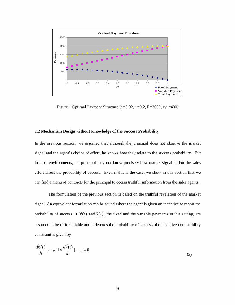
Figure 1 provides an example of the optimal payment functions when •=0.02, •=0.2, R=2000 and
xs0=400. For example, when success probability for the optimal effort is 0.5, the fixed payment is
469 and variable payment is 1375. However, when the probability is 0.6, the fixed payment
decreases down to 400 and the variable payment becomes 1500. This means that while the
probability of having a successful sales deal increases, agent’s fixed payment is reduced and her
variable payment is increased. Increases in the variable payment compensate decreases in the
fixed payment as p* (or equivalently, s) approaches to 1 and make their total an increasing
function.
)4/()*()2/()*)((*)(ˆ)2/()*(*)(ˆ
2222220
22
αβααβαβα
αβα
+−−+−−−=
−+=
RpRpRxpxpRpy
s
)2()(* 2 ββα −+= sRsp
)2/())(*( 2 ββα +−= Rsps
9
Optimal Payment Functions
0
500
1000
1500
2000
2500
0 0.1 0.2 0.3 0.4 0.5 0.6 0.7 0.8 0.9 1p*
Pay
men
t
Fixed PaymentVariable PaymentTotal Payment
Figure 1 Optimal Payment Structure (•=0.02, •=0.2, R=2000, xs0 =400)
2.2 Mechanism Design without Knowledge of the Success Probability
In the previous section, we assumed that although the principal does not observe the market
signal and the agent’s choice of effort, he knows how they relate to the success probability. But
in most environments, the principal may not know precisely how market signal and/or the sales
effort affect the probability of success. Even if this is the case, we show in this section that we
can find a menu of contracts for the principal to obtain truthful information from the sales agents.
The formulation of the previous section is based on the truthful revelation of the market
signal. An equivalent formulation can be found where the agent is given an incentive to report the
probability of success. If )(~ tx and )(~ ty , the fixed and the variable payments in this setting, are
assumed to be differentiable and p denotes the probability of success, the incentive compatibility
constraint is given by
0|)(~|)(~
=+ == ptptdt
tydpdt
txd(3)

10
Note that the contract menu is independent of the effort and the market signal once p is
given. Therefore, any menu of contracts that satisfies the condition above and that provides the
agent at least her reservation profit induces truth telling. Particularly, if we assume that )(~ tx is a
decreasing second-order quadratic function and )(~ ty is linearly increasing (as in the previous
section), using Equation (3) we find that
2)(~
2btctx −= (4)
btty =)(~(5)
where b and c are constants. Since the objective of the agent is concave with respect to t,
Equation (3) is also sufficient. A detailed analysis of the equilibria under )(~ tx and )(~ ty is given
in Proposition 3 of the Appendix.
Our main motivation to use in our experiments the above functional forms was to analyze
how they perform in terms of truth telling when they are presented to human subjects. Another
reason is to find out whether the principals can offer relatively “good” contracts to their agents
that will lead to higher efficiency and better information on the success probability of the sales, as
deals compared to traditional methods. Therefore, the principal is asked to choose the total
payment )(~)(~)( tytxtP += at t=0 and t=1 in our experiments. In order to simplify the
principal’s decision, the contract is then automatically filled in by the following equations
2))0()1(()0()(~ tPPPtx −−=
tPPty ))0()1((2)(~ −=
which is consistent with Equations (4) and (5).
It is beyond the scope of this paper to provide a theoretical model of how a rational
strategic principal will choose the contract since it involves modeling the principal’s beliefs about

11
the functional form, which can be very difficult. Instead we empirically test this approach with
human subjects.
2.3 Benchmark Model
We use a model that mimics a simplified version of a typical business scenario to serve as
the benchmark. In this scenario, the principal offers the agent a fixed payment that he will receive
regardless of his actions, plus a bonus that will be paid only in the case of success. The key
difference from the previous model is that both the fixed payment and the bonus are constant (i.e.,
the principal doesn’t provide the agent with a menu). In this setting, the principal minimizes the
function
Where es is a solution to the agent’s profit maximization problem that is given by
The bonus y is determined from solving both the agent’s and the principal’s problem,
whereas the fixed payment, x, is found from the least profit that the principal has to provide to the
agent.
Proposition 2: The optimal bonus is given by
If the amount of money paid to the agent (at a market signal of zero) in the principal-
agent model and in the benchmark model is set equal to each other, the fixed payment in the latter
is found by:
where xs 0 is the fixed payment at s=0.•
We can now compare the solution of the benchmark model and the principal-agent model
in terms of the agent’s and the principal’s expected profit. It is expected that when the principal
)]1,min()1,min([max , seyxseRE sssyx βαβα +−−+
}2/)1,min({max 2eseyxe −++ βα
)4/()2( 22 αβα −= Ry
)2/()()32/()2( 2222220 αβααβα −+−−= RRxx s

12
offers a menu of contracts, he will earn higher profits due to higher flexibility. If the optimal y
and x are such that
The difference in the principal’s expected profit between the original and the benchmark
model is given by:
The difference in the agent’s expected profit between the original and the benchmark
model is
Note that •p and •a are always positive once the conditions on the probabilities
are satisfied.
The differences in the expected profits indicate that both the agent and the principal are
better off under the proposed compensation mechanism. Furthermore, this mechanism has the
property of retrieving truthful information from the agent.
3. Experimental Design
The central point to be settled by the experiments is whether this mechanism can elicit non-biased
information even when humans may not behave exactly as economic theory prescribes. Another
issue to be elucidated is that the compensation mechanism depends on the assumption that the
principal knows the probability relation, a fact which is not often possible in real life.
222 /)96/7(8/)( αββα +−=∆ RRp
)24/()56( 22 αβαβ −=∆ Ra
1)()1(* 2 ≤+= βαRp
0)()0(* 2 ≥−= βαRp
)4/()2( 22 αβα −= Ry
)2/()()32/()2( 2222220 αβααβα −+−−= RRxx s

13
We conducted four sets of experiments: In the first set, a sales agent responds to a
software principal who always uses an optimal payment schedule. The second set comprised the
full principal-agent scenario where both the principal and the agent are human subjects. The third
set is the same as the full principal-agent scenario, but we also added the ability to have limited
communication between principals and agents before the contract setting stage. Finally, we used a
treatment where the contract consists only of a single, pre-determined fixed payment and bonus to
serve as a benchmark.
The experiments were implemented in the HP Experimental Economics Software
Platform, MUMS. The subjects (mostly students from Stanford University) played the role of
principals and sales agents. Standard HP Labs experimental economics procedures were
followed. The experimental model was implemented in the HP experimental economics software
platform and the experiments were conducted at the HP experimental economics laboratory.
Subjects were paid according to their performance in the experiments, most of them making in
the range of $50-$150 for an afternoon session. Before the subjects came into the lab, they had to
go through a set of web based instructions and then pass a quiz.
In Agent-only experiment, we informed the agent about the value of her market signal
and then, she decided on her report and her effort at each period. The market signal is
independently drawn from continuous uniform distribution between 0 and 1 at each period. The
sales agent was given the same menu of contracts (fixed and variable payment functions) over
time that is optimal for a specified set of parameters. Each agent was given two minutes to make
his decision. At the end of a period, the outcome of the sales deal was determined by a random
draw where the success probability is given by min(•e+•s,1). Sales agents may face nonpositive
fixed payments depending on the set of parameters used during the game.
In the Benchmark experiment, each period consisted of four stages: In the first stage of
the experiment, the principal set the fixed payment. In the second stage, the agent observed the

14
fixed payment and the market signal and she reported a value to the principal. The principal was
not informed about the market signal. The agent’s report, though does not directly affect agent’s
payments as they did before, was added to this experiment as a communication channel between
the principal and the agent. In the third stage, the principal determined the variable payment. In
the final stage, the agent chose her sales effort. The effort could not be observed by the principal
as well. Each stage lasted for one minute. Each principal was matched with three sales agents
working on separate sales deals at the beginning and played with the same agents through the
game.
In the Principal-agent experiment, the principal moved first and were asked to decide on
the total payment (fixed + variable payment) for the agent at the extreme range (0 and 1) of the
report. Fixed and variable payments for each possible report were then generated automatically to
enable truth telling. Once the payment menu was provided and the market signal was drawn as
before, the agent decided on the report and the effort. The principal could not see the market
signal or the effort of the agent. All the players were given two minutes to make their decisions.
Each principal was matched with the same set of agents for the whole experiment.
In two of our principal-agent experiments, each principal was matched with three sales
agents working on separate sales deals as in the benchmark experiment. Each principal played the
game with the same agents at each period. In the last principal-agent experiment, each principal
was matched in the first run and was randomly rematched in the second run with a single agent.
Principal-agent experiment with communication was the same as the principal-agent
experiments, except every five periods, the principals and agents were allowed to exchange
messages in the form of a possible contract ( i.e total payment at report 0 and 1 and effort values
when the market signal is 0, 0.5 and 1).
For all of the experiments, once the sales deal is revealed to be successful or not, a sales
agent‘s payoff is found by adding fixed payment and variable payment if the sales deal is

15
successful and subtracting the cost of effort. A principal’s payoff is found by subtracting the total
payment to the agent from principal’s sales revenue (0 if the deal is not successful). After each
period, the agents were given the following feedback information: Market signal at the last
period, their effort, their report, fixed and variable payment (corresponding to the report chosen
except for the benchmark experiments), an indicator showing the deal was successful or not,
payoff from the last period and cumulative payoff in the game. The principals were given a
summary of their payment decisions, their agent’s report, an indicator showing the deal was
successful or not, payoff from the last period and their cumulative payoff.
It is worth noting that in all of the experiments, a principal was matched with the *same*
set of agents for multiple periods. While this obviously introduced repeated game effects, we felt
is necessarily so as to provide the principals a better chance to learn to adjust the menu of
contracts for “their” agents. Because of the Folk Theorem, the mechanism can be even more
efficient than the theory has predicted. Thus, we stacked the deck in flavor of the theory. The
results reported below are even more shocking in light of this.
4. Results
A total of 10 experiments were conducted. The following table summarizes the experimental
settings. The first experiment was a pilot which provided a test of the software and procedures.
Table 1 Experiment overview
Experiment Date Type of the experiment# of
subjects# of
periods
1 08.05.2005Pilot experiment
10 50
2 08.22.2005 Agent-only 9 50
3 09.02.2005 Principal-agent 12 25
4 09.06.2005 Principal-agent 12 25
5 09.08.2005 Benchmark 12 25
6 11.03.2005 Benchmark 12 30

16
7 07.07.2006Principal-Agent
w/Communication 16 10
8 07.21.2006Principal-Agent
w/Communication 12 25
9 08.25.2006Principal-Agent
(Single) 10
20 at each run (2 runs)
Result 1: The truth telling contract solicit at least as much information from the agents as in
the benchmark contract. R-squared between the reported probabilities of success and the truth
probabilities of success is used as the primary measure of information revelation. We calculated
this measure pooling all of the observations from each experiment.
The following example illustrates why this measure was chosen. Consider an agent
consistently reporting a*(probability of success), where a is a constant between 0 and 1. If we use
any measure based on absolute accuracy, we will obtain different results depending on a. If a is
known however, the principal can back out a perfect forecast every time. Thus, this particular
rule-of-thumb actually reveals all the information the agent has. The R-squared measure for this
particular rule-of-thumb is always 100%, thus capturing all of the information that is revealed.
Table 2: R-squared of True Probability and Report
Experiment TreatmentR-
squared1 Agent-only 0.612 Agent-only 0.873 Principal-Agent 0.694 Principal-Agent 0.80
5PA with
Communication 0.50
6PA with
Communication 0.407 Benchmark 0.308 Benchmark 0.629 Single PA 0.36

17
10 Single PA 0.29
As one can see from table 2, out of the four agent-only and principal-agent experiments,
three have higher R-squared than the two benchmark experiments. One out of those four has R-
squared very close to one of the benchmark experiment and higher than the other one.
However, the principal-agent experiment with communication and the principal-agent
experiment where single principal was matched with a single agent did not do so well with
respect to information revelation. All of these four experiments have lower R-squared than the
benchmark ones.
The surprising result is not so much as how the truth-telling contract performed, but that a
fair amount of information was revealed in the benchmark experiments. Note that there is no
incentive, in the one-period game, for agents to reveal any information in the benchmark
experiment. Since the same principal was paired with the same agent in the experiments,
reputation effect would encourage some information sharing. The surprise here is that properly
designed truth-telling contract did not seem to have a significant advantage over the benchmark
scenario when the game was repeated.
Result 2: Nonlinear behavior with respect to probability reporting was observed. In many
instances, subjects were observed to under-report in low-probability ranges and over-report in
very high-probability ranges. The following figure illustrates this phenomenon.
Figure 2 Example of the S-structure

18
As can be seen, the data follows an S shape curve. One explanation of this behavior is
that when the optimal report is low and there is a small to moderate chance of ending up with a
successful deal, risk-averse subjects prefer to report low and gain from the fixed payment. On the
other hand, when the probabilities of success is higher, subjects report high and try to take
advantage of high variable payments. This means that risk considerations make the subjects
deviate from maximizing their expected earnings.
To determine the extent of this behavior; we estimated a polynomial regression model
with the report as the dependent variable and the truth probability as the independent variable. We
found that in five out of ten experiments, the model is significant in the square or the cubic term
of the polynomial, showing that the response is not linear at least in some of the experiments.
In addition, we found that clustering of the data points at the high and low end was quite
common, and we observed this in the data for true probability vs. report as well. This can be
understood from the subjects’ relation with effort and probability: subjects choose low effort
when the signal is small, which makes the probability of success small and report a low value as
well. When the signal takes a moderate value, they choose a high effort that also increases the
probability of success. As the signal becomes larger, even if they show a moderate effort, they

19
end up having a high probability value. The last two cases can be the explanation to the clustering
at the high end while the first one explains the clustering in the low end.
Figure 3 Examples of Clustering
Result 3: The truth-telling contract caused significant under-reporting. In additional to
nonlinear behavior, we found that subjects had a tendency to report probabilities lower than the
truth. A paired Wilcoxon signed rank test was used to determine if the reported probabilities are
LOWER than the true ones. The following table summarizes the results.
Table 3: P-values of Wilcoxon Signed Rank Test for alternative that Reported Probabilities <
True Probabilities
Experiment Treatment P-value1 Agent-only <0.00012 Agent-only <0.00013 Principal-Agent <0.00014 Principal-Agent <0.0001
5PA with
Communication 0.0221
6PA with
Communication <0.00017 Benchmark 1.00008 Benchmark 1.00009 Single PA 0.0002

20
10 Single PA 0.0005
As one can see, the test rejected the hypothesis, with very high significance, in favor of
the alternative that the reported probabilities were LOWER than the true ones in all the
experiments using the truth-telling contract. Worth noting that the null hypothesis that the
reported probabilities were not smaller than the true ones cannot be rejected in both benchmark
experiments. This is strong evidence that the contract was the cause of this lower-reporting
phenomenon.
Result 4: The benchmark scenario resulted in significant over-reporting. We found that
subjects had a tendency to report higher probabilities in the benchmark experiments. A paired
Wilcoxon signed rank test was used to determine if the reported probabilities are HIGHER than
the true ones. The following table summarizes the results.
Table 4: P-values of Wilcoxon Signed Rank Test for alternative that Reported Probabilities >
True Probabilities
Experiment Treatment P-value7 Benchmark <0.00018 Benchmark <0.0001
In the context of the period game, probability reporting in the benchmark experiments
was cheap talk. Hence, there is no theoretical prediction. In the repeated game context, Folk
theorem also does not provide clear unique predictions. Thus, we are left with little guidance
from standard theory to interpret this result.
On the other hand, intuitively, this result is not difficult to understand. The agents had the
incentive to paint a rosier picture in the hopes that the principals would increase their bonus. This
explanation implies that the agents believe that principals would react to their reports naively.
Result 5: The truth-telling contract was NOT as efficient as the benchmark scenario. The
following table summarizes the average payoff and the efficiency of each experiment.

21
Table 5: Payoffs and efficiencies
Experiment Treatment
AveragePayoff
Average Expected
Payoff
EquilibriumExpected
PayoffEfficiency
1 Agent-only 370.34 361.48 410.59 0.88
2 Agent-only 15629.88 15790.08 17039.03 0.93
3 Principal-Agent 12202.25 12820.47 16863.46 0.76
4 Principal-Agent 11610.15 12501.93 16137.89 0.77
5PA with
Communication 11772.60 13755.27 17926.87 0.77
6PA with
Communication 11473.97 12578.08 17002.53 0.74
7 Benchmark 13023.41 13700.96 14118.33 0.97
8 Benchmark 16011.95 13370.56 14809.87 0.90
9 Single PA 15827.79 13792.56 17788.24 0.78
10 Single PA 12428.27 12065.76 16914.42 0.71
The efficiency was calculated based on average EXPECTED payoff. We used the
expected payoff based on subjects’ decisions, as opposed to using the actual realized payoff.
Thus, this is a measurement of the value of their decisions.
As one can see, the two benchmark experiments have the higher efficiencies than all
principal-agent experiments. The probability that the two benchmark experiments have higher
efficiencies than all 6 principal-agent experiments, if ordering of the experiments based on
efficiencies is random, is (2! 6!)/8! ~ 3%.
The efficiencies of the two agent-only experiments are similar to that of the benchmark
experiments. Thus, the low efficiencies in the principal-agent experiments were likely to be
caused by the subjects’ inability to offer the right contract.
Note that the value of the forecast was not factored into this analysis and we assume there
are some exogenous reasons why accurate forecasts are desired.

22
Result 6: Communication did increase neither information revelation nor efficiency. As
shown in the table above, the treatment where principal-agent communication was allowed did
not result in a significant improvement in information revelation or efficiencies. Thus, it is
unlikely that the low performance of the truth-telling contract was due to a lack of
communication between subjects.
5. Conclusions and Future Research
Central to whether principal-agent mechanisms can be made practical, is whether the game theory
model is robust with respect to the stringent rationality requirements imposed upon the decision
makers. For example, we employed the solution concept of the Bayesian Nash equilibrium to
predict how people behave in this mechanism. The solution requires the principal to have perfect
knowledge of the probability relation of effort, market signal and the outcome (i.e. the deal is
successful or not) and relevant utilities function for themselves, and then determine the best
contract schedule by solving mathematical equations. The agents are assumed to be risk-neutral
expected utility maximizers who also solve complex mathematical problems before arriving at the
decisions. This is obviously beyond the undertaking of even the most sophisticated managers and
sales agents. Furthermore, there is ample evidence to show that people are neither risk-neutral nor
even adhering to expected utility maximization. The real question is whether theory is a good
enough approximation so that the insight gained, mainly the use of menu of contracts to solve the
problem of information asymmetry, is robust to behavioral effects.
In this paper, we explored behavioral issues with respect to the application of principal-
agent type mechanisms to the sales forecasting problem. While human subject experiments
showed that a properly designed mechanism can elicit reasonable amount of information, we
observed substantial behavioral deviations from model predictions. In particular, we found that
subjects tends to over-estimate high probabilities (>0.5) and under-estimate low ones. In addition,
managers tended to underpay their agents and that resulted into lower levels of effort.

23
The research reported here provides answers along two dimensions that were not
previously addressed. First, we expanded the scope of the agency problem to include soliciting
truthful forecasts from the agents. Second, we solved this problem endogenously with respect to
choosing the menu of contracts. While the true principals, i.e., the managers of the sales force,
may not have either the data or the analytical skills to estimate the relevant functions and derive
the subsequent optimal solutions, we created a mechanism that allows them to learn the solution
through repeated interaction with the agents. Our results suggest that it is not enough to address
the issue of principals’ lack of knowledge of functional dependencies and that the mechanism
design process needs to incorporate behavioral effects.
There are two possible future directions of this research. First, we are planning to
redesign the mechanism with respect to behavioral issues. In addition, there are many additional
variations in the environment, such as information discovery, multiple deals, soliciting a revenue
forecast instead of a probability of success, and multiple agents working on the same deal.
Additional research will be needed to develop a mechanism to adapt to these characteristics.
Another direction is to explore a field test within a real business to further investigate
whether behavioral effects observed inside the lab will be consistent with real business
environments. This obviously would be much further down the road since it is less likely a
business is willing to subject itself to new processes unless there is some evidence that it will
provide additional value.
Nevertheless we feel that this study elucidates a number of problems with principal agent
theory which offer plausible reasons as to why contracts designed through standard principal-
agent models are seldom used in practice.
24
REFERENCES
Anderhub, V., Gachter, S. and Konigstein, M., 2002. Efficient Contracting and Fair Play in a
Simple Principal-Agent Experiment. Experimental Economics, 5, 5-27
Berg, J.E., Daley, L.A., Dickhaut, J.W., and O-Brien, J., 1992. Moral Hazard and Risk Sharing:
Experimental Evidence. Research in Experimental Economics 5, 1-34
Bolton, P., and Dewatripont, M., Contract Theory, MIT Press
Cabrales, A. and Charness, G., 2003. Optimal Contracts, Adverse Selection and Social
Preferences: An Experiment, Mimeo
Chen, K-Y, Fine, L., Huberman, B. 2004. Eliminating Public Knowledge Biases in Information-
Aggregation Mechanisms. Management Science, Vol. 50, No. 7, 983-994
Epstein, S., 1992. Testing Principal-Agent Theory, Experimental Evidence. Research in
Experimental Economics 5, 35-60
Ghosh, M. and John, G. 2000. Experimental Evidence for Agency Models of Salesforce
Compensation. Marketing Science, Vol. 19, 348-365.
Holmstrom, B. 1979. Moral Hazard and Observability. Bell J. Econ. Vol 10, 180-191 (1979)
Keser, C., and Willinger, M., 2000. Principals’ Principles when Agents’ Actions are Hidden.
International Journal of Industrial Organization, 18,1, 163-185
Keser, C., and Willinger, M., 2002a. Theories of Behavior in Principal-agent Relationships with
Hidden Action, Working Paper BETA no. 202-07, University Louis Pasteur, Strasbourg
Keser, C., and Willinger, M., 2002b. Experiments on Moral Hazard and Incentives, in The
Economics of Contracts: Theory and Applications, ed. By E. Brousseau and J.M Glachant.
Cambridge University Press
Laffont, J., and Martimort, D., 2002. The Theory of Incentives, Princeton University Press

25
Milgrom, P. 1991. Multi-task Principal Agent Analyses: Incentive Contracts, Asset Ownership
and Job Design. J. Law, Econom. Organ. Vol. 7, 24-52
Segal, I. 2006. “Lecture Notes in Contract Theory”, Department of Economics, Stanford
University
Staelin, R. 1986 Salesforce Compensation Plans in Environments with Asymmetric Information.
Marketing Science, Vol. 5, 179-198
APPENDIX:
Note that 0,, >Rβα in our models. The following lemma will be used when we identify the
optimal solution to the principals’ problem:
Lemma 1: Equation 2 is satisfied if and only if the following conditions hold:
(C1) ∫+=≡Φs
dyUsUss0
)()0()(),( ττβ
(C2) y(s) is nondecreasing in s
Proof of Lemma 1: We begin by showing that the IC constraints imply (C1) and (C2). We can
rewrite the IC constraints as )}(),ˆ({maxargˆ sUsss s −Φ∈ where
2)()()(),()(
22 syssysxsssU αβ ++=Φ= . This implies that
)ˆ(|/),ˆ(|/)( ˆˆ sysssdssdU ssss β=∂Φ∂= == . Using the Fundamental Theorem of Calculus, we
have
∫+=s
dyUsU0
)()0()( ττβ.

26
To see how IC constraints imply y(s) to be nondecreasing in s, we compare the IC conditions for
s and s where ss ≤ˆ :
They can be rewritten as:
Since ss ≤ˆ , the inequality above implies that )()ˆ( sysy ≤ .
We will now show that (C1) and (C2) imply IC constraints. We define the net benefit from
reporting s when the agent observes s as
)(),ˆ(),ˆ( sUssss −Φ=φ
If both sides of the equation are differentiated with respect to s for a fixed s , we get
)()ˆ(/)(/),ˆ(/),ˆ( sysydssdUssssss ββφ −=−∂Φ∂=∂∂
Note that if ss <ˆ , 0/),ˆ( ≥∂∂ sssφ , while if ss ˆ< , 0/),ˆ( ≥∂∂ sssφ . Therefore, this function
is maximized when ss ˆ= and IC is satisfied.
Proof of Proposition 1: We can define ),( ste as:
}2
))(()({maxarg),(2esetytxste e −++∈ βα
Note that we assume •e(t,s)+•s does not exceed 1. We solve for the agent’s best response and
principal’s maximization program under this assumption. We check whether the solution we find
satisfies the assumption.
2)(ˆ)()(
2)ˆ(ˆ)ˆ()ˆ(
2222 syssysxsyssysx αβ
αβ ++≥++
2)ˆ()ˆ()ˆ(
2)()()(
2222 syssysxsyssysx αβαβ ++≥++
2)()(
2)ˆ()ˆ()ˆ()(
2)(ˆ)(
2)ˆ(ˆ)ˆ(
22222222 syssysyssysxsxsyssysyssy αβαβαβαβ −−+≥−≥−−+
ssysyssysy ββ ))()ˆ((ˆ))()ˆ(( −≥−

27
The first-order condition to find the optimal effort given the report t and signal s is given by:
Since the agent’s expected profit given the report and the signal is concave in the effort, this first-
order condition is also sufficient. Hence, the agent’s maximum profit given that he observes s and
reports t is found from:
2)()()(
2)())()(()(),(
22222 tystytxtystytytxst α
βα
βα ++=−++=Φ
The expected payments from the principal to an agent of type s are
Since the payments can be increased and the objective can be improved when uU >)0( , in the
optimal solution it must be the case that uU =)0( . Using the relation above, we can write the
principal’s objective as
})2
)()())((({max22
0
1
0
2() dssydyussyR
s
yα
ττββα −−−+ ∫∫
s.t (C2)
We can omit u for optimization purposes. The objective can then be rewritten using integration by
parts:
})2
)()()1())((({max221
0
2() dssysysssyRy
αββα −−−+∫
We first find the solution to the problem by relaxing the constraint (C2) and later check if that
condition is satisfied. Optimal solution to the relaxed problem found by pointwise maximization
is given by
2)()()0(
2)()())()(()(
22
0
222 sydyUsysUssysysx
s αττβ
αβα ++=+=++ ∫
ety =α*)(

28
Since this is a nondecreasing function of s, (C2) is satisfied and the solution is optimal for the
principal’s problem. Using this function and the agent’s expected profit )(sU , x(s) is given as
where xs0 is the fixed payment part of the contract when the report (or similarly, the market
signal) is 0. We will use xs0 as a parameter in our experiments instead of the reservation profit u
for simplicity.
Under y(s) and x(s) found here, agent’s profit function is jointly concave with respect to t
and e. Hence, first-order conditions are sufficient once •e(s,s)+•s does not exceed 1 and t • [0,1].
•e(s,s)+•s does not exceed 1 for all s for the parameter sets we used in our experiments
( 40000,, =0.5=0.00353553= Rβα in all experiments except for the pilot agent-only
experiment, 1000,4,23 =0.=0.0= Rβα for the pilot experiment). Hence, the equilibrium we
find is valid. Since we use the solution found here in agent-only experiments and provide the
subjects with the menu to which they have a unique best-response (under expected profit
maximization), we omit further discussion on other possible equilibria. •
Proof of Proposition 2: We first fully characterize the equilibria under the benchmark model.
Agent’s objective is
e will not be set such that αβ /)1( se −> since the effort is costly and additional effort will not
increase the probability. Therefore, we can rewrite the problem as
First-order conditions are given by
0/ =−=∂∂ eyea απ
)/()()( 22 αββα −+= sRsy
222220 /)/()( αβαββ ssRxsx s −−−=
}2/)1,min({max 2eseyxe −++ βα
}2/)1,min({max 2/)1(0 eseyxsea −++= −≤≤ βαπ αβ

29
01/ 22 <−=∂∂ eaπ
Note that the objective is concave in e. Optimal effort is found to be
)/)1(,min(),(* αβα syyse −=
Principal’s objective can be written as
∫ −+−1
0
, })),(*)({(max dsxsyseyRyx βα
Define sb as
βααβα /)1(/)1( 2 yssy bb −=⇒−=
We consider three cases based on the value of sb:
Case 1: αβ /)1(),(*0 sysesb −=⇒<
In this case, principal’s maximization problem turns into
)/(1y0/)y1(t.s)xyR(max 22y,x α≥⇒≤βα−−−
Since the objective is decreasing in y, y is chosen to be equal to 1/(•2).
Case 2: yysesb α=⇒> ),(*1
In this case, principal’s maximization problem can be written as
1/)y1( t.s x)yR(2/1y)yR(ds}x)sy)(yR{(max 221
0
2y,x ≥βα−−β−+α−=−β+α−∫
First-order condition is given by
)4/()2(02/2 2222 αβαβαα −⇒=−− RyR
Since the second-order condition is negative, principal’s objective is concave in y.

30
Taking the bounds on y into consideration, optimal y is found from
)}/()1()},4/()2(,0min{max{ 222 αβαβα −−= Ry
Case 3: 10 ≤≤ bs
In this case, principal’s maximization problem can be written as
222
20
12
,
/1/)1(1/)1(0.
)1)((2/)()(
)(}))({(max
2
ααββα
βα
βα
≤≤−⇒≤−≤
−−−+−−+−=
−−+−+−∫ ∫
yyts
sxyRxssyRysyR
dsxyRdsxsyyR
bbbb
s
s
yx
b
b
First-order condition is given by
0)2/()1)()32(1(1 22 =+−−+−− βαα yyR
Since the first-order condition at 2/1 α=y is negative, this point can be eliminated. Therefore,
the optimal solution in this case is found by comparing the objective values of 2/)1( αβ−=y
(lower bound on y) and y we find from the first-order condition.
Optimal y to principal’s problem is found by comparing the optimal solutions at each case.
For the parameter set 40000,, =0.5=0.00353553= Rβα (which is the parameter set we used
in our benchmark, principal-agent and principal-agent with communication experiments), Case 2
becomes optimal and )4/()2( 22 αβα −= Ry . Optimal effort of the agent is found
by ye α=* .•
Proof of Proposition 3:
Agent’s problem can be written as
010
.}2/)1,min(2/{max 22
,
≥≤≤
−++−
et
tsesebtbtcet βα

31
e will not be set such that αβ /)1( se −> since the effort is costly and additional effort will not
increase the probability. Therefore, we can rewrite the problem as
The objective is jointly concave in t and e when 2/10 α≤≤ b . In this case, optimal t* and e* are
given by
}/)1(,min{**
αβαβα
stbeset
−=+=
The agent’s best response is
)1/(* 2ααβ bsbe −= and set βα += ** if 22 /10,/)1()1/()( ααβαβα ≤≤−≤− bsbsb
αβ /)1(* se −= and 1* =t if 22 /10,/)1()1/()( ααβαβα ≤≤−≥− bsbsb
The principal’s problem can be written as
})2/)(*))(*))((*(({,max 21
0
dssbtcssesbtRbc +−+−∫ βα
We can omit c for optimization purposes. We define sd to be the point where
αβααβ /)1()1/( 2 sbsb −=− . ( βα /)1( 2bsd −= )
Based on the principal’s objective, there are three cases:
Case 1: 1*,/)1(*0 =−=⇒< tsesd αβ
In this case, principal’s maximization problem turns into
αβ
βα
/)1(010
.}2/)(2/{max 22
,
set
tsesebtbtcet
−≤≤≤≤
−++−

32
)/(10/)1(.
)2/(max
22 αβα ≥⇒≤−
−
bbts
bRb
Since the objective is decreasing in b, b is chosen to be equal to 1/(•2). Principal’s expected profit
is R-1/(2•2).
Case 2: setbsbesd βααβα +=−=⇒> **),1/(*1 2
In this case, principal’s maximization problem can be written as
)/()1(0.
}2/))1/(())1/())()1/(({(max
2
1
0
2222222,
αβ
βαβαβαβαβαβα
−≤≤
+−++−+−−∫
bts
dssbsbbsbsbsbsbbRyx
First-order conditions of the principal’s objective is given by
0)1/()33())1(6/()3( 322222222 =+−+−+−+− ααβββααββα bbRbRbR
The solution to this equation is ))3(/()3( 222 βααβα +−= RRb .
Note that the derivative of the principal’s objective at b=0 is positive when all of the parameters
are positive. Therefore, this point is eliminated.
Objective value at ))3(/()3( 222 βααβα +−= RRb and )/()1( 2αβ−=b must be compared
if )/()1())3(/()3( 2222 αββααβα −≤+− RR . If the condition is not satisfied, the only
candidate solution is )/()1( 2αβ−=b .
Case 3: 22 /1/)1(10 ααβ ≤≤−⇒≤≤ bsd
In this case, principal’s maximization problem can be written as

33
22
1
0
2222222
/1/)1(.
)2/(
}2/))1/(())1/())()1/(({(max
ααβ
βαβαβαβαβαβα
≤≤−
−+
+−++−+−−
∫
∫
bts
dsbR
dssbsbbsbsbsbsbbR
d
d
s
s
b
First-order conditions of the principal’s objective is given by
0)6/())2(3)1)(32(( 2 =−++−−− ββα RbbRb
The solution to this equation is )4/())(32( 22 αβα −+= Rb .
Since the second-order condition is 0)3/()2( 2 <− βα , the function is concave with respect to b.
Hence, once the solution found from the first-order conditions is in the bounds, it is optimal for
this case. Otherwise, we need to compare the objective values at bounds )/()1( 2αβ− and
)/(1 2α .
For the parameter set 40000,, =0.5=0.00353553= Rβα (which is the parameter set we used
in our benchmark, principal-agent and principal-agent with communication experiments), Case 2
becomes optimal and 40000=b . •