does money buy happiness? a longitudinal study … does money buy happiness? a longitudinal study...

Does Money Buy Happiness? A Longitudinal StudyUsing Data on Windfalls

Jonathan GardnerDepartment of Economics

Warwick UniversityCV4 7AL

[email protected]

Andrew OswaldDepartment of Economics

Warwick UniversityCV4 7AL

[email protected]

March 2001

For their helpful ideas, we are grateful to Danny Blanchflower, Andrew Clark, Ed Diener, Jane Hutton, BruceSacerdote, Jon Skinner, Alois Stutzer, and Ian Walker. The Economic and Social Research Council providedresearch support.

Abstract

The most fundamental idea in economics is that money makes people happy. This

paper constructs a test. It studies longitudinal information on the psychological

health and reported happiness of approximately 9,000 randomly chosen people. In

the spirit of a natural experiment, the paper shows that those in the panel who

receive windfalls -- by winning lottery money or receiving an inheritance -- have

higher mental wellbeing in the following year. A windfall of 50,000 pounds

(approximately 75,000 US dollars) is associated with a rise in wellbeing of between

0.1 and 0.3 standard deviations. Approximately one million pounds (1.5 million

dollars), therefore, would be needed to move someone from close to the bottom of a

happiness frequency distribution to close to the top. Whether these happiness

gains wear off over time remains an open question.

1

Does Money Buy Happiness? A Longitudinal Study Using Data on Windfalls

Jonathan Gardner and Andrew Oswald

1. Introduction

The central tenet of economics is that money makes people happy. Using deduction,

rather than evidence, economists teach their students that utility must be increasing in

income1. In this paper we construct one of the first empirical tests. Our results, using two

measures of mental wellbeing, show that the economist’s textbook view is correct. We

also estimate the size of the effect of a windfall on wellbeing.

To make persuasive progress on this problem, data with three special features are

required. First, it is necessary to have a panel of people, that is, longitudinal rather than

purely cross-sectional information. Second, measures of psychological wellbeing are

needed. Third, it is necessary to observe, whether by an actual or natural experiment, a

random assignment of money amongst individuals. We have a data set that approximates

these conditions. As far as we know, previous investigators in economics or psychology

have been unable to implement such a test. Diener and Biswas-Diener (2000) argue that

this form of research design is required.

Individuals' survey responses to questions about wellbeing are used in the paper.

Such responses have been studied before. They have been used intensively by

psychologists2, examined a little by sociologists and political scientists3, and largely ignored

by economists4. Some economists may emphasise the likely unreliability of subjective data

1 A common approach would be to argue that more income simply must make people happier because itopens up extra choices that are denied those with less money; yet in principle human beings might find itcostly to make more decisions about how to spend the greater income. Another argument might be thatpeople seek more income whenever they can, so that it necessarily makes them happier; yet in principle theycould be mistaken about how they will feel ex post. However, the best reason to want empirical evidence isthat it is dangerous for any subject to reach the point where it cannot be conceived that a familiarassumption might be wrong.2 Earlier work includes Andrews (1991), Argyle (1989), Campbell (1981), Diener (1984), Diener et al (1999),Douthitt et al (1992), Fox and Kahneman (1992), Larsen et al (1984), Mullis (1992), Shin (1980), Veenhoven(1991, 1993), and Warr (1990).3 For example, Inglehart (1990) and Gallie et al (1998). There is also a related empirical literature oninteractions between economic forces and people’s voting behavior; see for example Frey and Schneider(1978).4 The recent research papers of Andrew Clark, Bruno Frey and Yew Kwang Ng are exceptions (Clark, 1996;Clark and Oswald, 1994; Frey and Stutzer, 1998, 1999; Ng, 1996, 1997). See also Frank (1985, 1997),

2

– perhaps because they are unaware of the large literature by research psychologists that

uses such numbers, or perhaps because they believe economists are better judges of human

motivation than those researchers. A recent literature on the border between economics

and psychology, however, has attempted to understand the patterns in happiness and stress

data.

2. Wellbeing Patterns

One definition of happiness is the degree to which an individual judges the overall quality

of life in a favourable way (Veenhoven, 1991, 1993).

Self-reported wellbeing measures are thought to be a reflection of at least four

factors: circumstances, aspirations, comparisons with others, and a person's baseline

happiness or disposition (e.g. Warr, 1980, Chen and Spector, 1991). Konow and Earley

(1999) describes evidence that recorded happiness levels have been demonstrated to be

correlated with:

1. Objective characteristics such as unemployment.

2. The person’s recall of positive versus negative life-events.

3. Assessments of the person’s happiness by friends and family members.

4. Assessments of the person’s happiness by his or her spouse.

5. Duration of authentic or so-called Duchenne smiles (a Duchenne smile occurs

when both the zygomatic major and obicularus orus facial muscles fire, and

human beings identify these as ‘genuine’ smiles).

6. Heart rate and blood pressure measures responses to stress.

7. Skin-resistance measures of response to stress.

8. Electroencephelogram measures of prefrontal brain activity.

Rather than summarise the psychological literature’s assessment of wellbeing data, this

paper refers readers to the checks on self-reported happiness statistics that are discussed in

Blanchflower and Freeman (1997), Blanchflower and Oswald (1998, 1999), Blanchflower, Oswald and Warr(1993), MacCulloch (1996), Di Tella and MacCulloch (1999), and Di Tella et al (2001). Offer (1998) containsinteresting ideas about the post-war period and possible reasons for a lack of rising wellbeing inindustrialised society.

3

Argyle (1989) and Myers (1993), and to psychologists’ articles on reliability and validity,

such as Fordyce (1985), Larsen, Diener, and Emmons (1984), Pavot and Diener (1993),

and Watson and Clark (1991).

Assume a reported wellbeing function:

(1) r = h(u(y, z, t)) + e

where r is some measure of psychological stress or self-reported number or wellbeing level

(perhaps the integer 4 on a satisfaction scale, or “very happy” on an ordinal happiness

scale), u(…) is to be thought of as the person’s true wellbeing or utility, h(.) is a continuous

non-differentiable function relating actual to reported wellbeing, y is real income, z is a set

of demographic and personal characteristics, t is the time period, and e is an error term. It

is assumed, as seems plausible, that u(…) is a function that is observable only to the

individual. Its structure cannot be conveyed unambiguously to the interviewer or any other

individual. The error term, ε, then subsumes among other factors the inability of human

beings to communicate accurately their happiness level (your ‘two’ may be my ‘three’).5

The measurement error in reported wellbeing data would be less easily handled if wellbeing

were to be used as an independent variable. This approach might be viewed as an

empirical cousin of the experienced-utility idea advocated by Kahneman et al (1997).

It is possible to view some of the self-reported wellbeing questions in the

psychology literature as assessments of a person’s lifetime or expected stock value of future

utilities. Equation 1 would then be rewritten as an integral over the u(…) terms. This

paper, however, will use stress and happiness questions on the assumption they describe a

flow rather than a stock.

Easterlin’s seminal research (1974, and more recently 1995) examined the reported

level of happiness in the United States. The author viewed people as getting utility from a

comparison of themselves against others; this is the idea that happiness has a large relative

component. Hirsch (1976), Scitovsky (1976), Layard (1980), Frank (1985, 1999) and

Schor (1998) have argued a similar thesis; a different tradition, with equivalent

implications, begins with Cooper and Garcia-Penalosa (1999) and Keely (1999).

5 This recognises the social scientist’s instinctive distrust of a single person’s subjective ‘utility’. Ananalogy might be to a time before human beings had accurate ways of measuring people’s height. Self-reported heights would contain information but be subject to large error. They would predominantly beuseful as ordinal data, and would be more valuable when averaged across people rather than used asindividual observations.

4

3. Data

The data used in this study come from the British Household Panel Survey (BHPS). This

is a nationally representative sample of more than 5,000 British households, containing

over 10,000 adult individuals, conducted between September and Christmas of each year

from 1991 to 1998. Respondents are interviewed in successive waves; if an individual

splits off from their original household, all adult members of their new household are also

interviewed. Children are interviewed once they reach 16. The sample has remained

representative of the British population throughout the 1990s.

The BHPS contains a standard mental wellbeing measure, a General Health

Questionnaire (GHQ) score. This is used by medical researchers and psychiatrists as a

measure of stress or psychological distress. It is unfamiliar to some economists, but GHQ

is probably the most widely used questionnaire-based method of measuring mental stress.

In the spirit favoured by psychologists, it amalgamates answers to the following list of

twelve questions, each one of which is itself scored on a four-point scale for 0 to 3:

Have you recently:

1. Been able to concentrate on whatever you are doing?

2. Lost much sleep over worry?

3. Felt that you are playing a useful part in things?

4. Felt capable of making decisions about things?

5. Felt constantly under strain?

6. Felt you could not overcome your difficulties?

7. Been able to enjoy your normal day-to-day activities?

8. Been able to face up to your problems?

9. Been feeling unhappy and depressed?

10. Been losing confidence in yourself?

11. Been thinking of yourself as a worthless person?

12. Been feeling reasonably happy all things considered?

5

We use the responses to these so-called GHQ-12 questions. For the first measure of mental

wellbeing, we take the simple sum of the responses to the twelve questions, coded so that

the response with the lowest wellbeing value scores 3 and that with the highest wellbeing

value scores 0. This approach is sometimes called a Likert scale and is scored out of 36.

The GHQ measure of stress, or lack of wellbeing, thus runs from a worst possible outcome

of 36 (all twelve responses indicating very poor psychological health) to a minimum of 0

(no responses indicating poor psychological health). In general, medical opinion is that

healthy individuals will score typically around 10-13 on the test. Numbers near 36 are rare

and usually indicate depression in a formal clinical sense.6

A second measure is used in the paper. We also study a direct happiness question.

This is Q12 above, denoted GHQH; so our happiness measure is in fact one twelfth of the

GHQ measure. We assume that this is a sufficiently small proportion to be ignored

without re-calibrating GHQ on only eleven questions.

We therefore employ a measure of (un)happiness as well as the mental stress

measure described earlier. The GHQH question is: have you been feeling reasonably

happy all things considered? This is the second measure of mental wellbeing. It is coded so that

high numbers denote more unhappiness.

A key requirement for a test is that something approximating a random drop of

money occurs. In a giant laboratory setting, this could be created experimentally. Aside

from any ethical considerations, such an experiment at the start of the 21st century is

probably infeasibly expensive to run. An equivalent is needed.

This paper relies on a natural experiment created by windfalls. The data contains

two sources of these – lottery wins and inheritances. These figures refer to windfalls

‘within the last year’, as assessed by the respondents. Lottery wins throughout the paper

include other gambling wins such as on the soccer ‘pools’. A huge percentage of the

British population play the national lottery, and small wins are common. Hence for

simplicity, because they dominate the data, we talk primarily of the lottery. The

inheritance variable includes both bequests and inherited property [it excludes receipts of

gifts or other private income transfers]. Despite the potential usefulness of lottery data to

economists and psychologists, the literature exploiting lottery information is still a

6 Likert is 12 times a number from zero to three. An alternative is the Caseness score, which counts the

6

comparatively small one. Most work has looked at how consumption and work choices are

affected by winning (for example, Bodkin 1959, Holtz-Eakin, Joulfaian and Rosen 1993,

Imbens, Rubin and Sacerdote 2000, Kaplan 1985, Kreinin 1961, Landsberger 1963, and

Sacerdote 1996). One well-known study in the psychology literature is Brickman, Coates

and Janoff-Bulman, 1978. This uses only a tiny cross-section sample of lottery winners,

and concludes that winners are slightly happier than those who do not win, but that the

difference is not statistically significant. Smith and Razzell, 1975, examined a cross-

section of those who won on football betting (the ‘pools’), and found that there was some

evidence of higher recorded happiness; but individuals also reported lower wellbeing in

other spheres of life.

There is an important disadvantage to our data set. Although the British panel

itself goes back to the start of the 1990s, questions on windfalls are new. Information on

the size of windfalls is known only for the 1997 and 1998 survey years. Analysis is

therefore restricted to that sample period7. These data are augmented with people’s GHQ

scores from prior waves, so as to allow the examination of how windfalls affect both the

level of wellbeing and how it changes over time. In other words, we are able to examine

long lags on the dependent variable. In the panel equations, we then have only two years

with which to examine the effect of windfall gains.

4. Results

Table 1 presents the simplest results. In these bivariate regressions, money does buy

greater happiness and lower measured stress.

Rises in wellbeing, to be clear about the choice of units and definitions, are given

by declines in GHQ mental stress and in GHQH unhappiness. This follows the standard

usage in the psychology and medical literature. Hence if money buys happiness, that

shows up in the paper’s tables as negatives on windfall coefficients.

number of times, out of twelve, that an individual answers in one of two negative response categories.7 There is one other piece of information. In 1995, people were asked whether they had received a windfall.This is used as a control variable in some of the regression equations.

7

Windfalls are associated with a statistically well-determined improvement in

wellbeing. Mental stress (GHQ) and unhappiness (GHQH) both decline in the year after a

windfall. This effect is found in the cross-sectional levels and in the panel’s changes.

In the cross-section equations, a windfall dummy (that is, whether the individual

had either an inheritance or lottery win) enters negatively for the full sample in both a

mental stress equation and an unhappiness equation. In the first columns of Tables 1a and

1b, the t-statistics are, respectively, 2.83 and 1.24. Entering the amount of windfall gives,

predictably, results that are better determined. This is column 2 of Tables 1a and 1b.

When only windfall recipients are studied, in column 3, the size of the windfall enters with

the expected negative sign and it is possible in each of Table 1a and 1b to reject the null of

zero at normal confidence levels.

The pure longitudinal effect of a windfall is picked up in the first-difference

equations in the last three columns of Tables 1a and 1b. Here the two dependent variables

are the change in mental stress GHQ and the change in reported unhappiness GHQH.

Person fixed-effects, therefore, have been removed. In five of these six equations, it is

possible to reject the null of zero on the windfall variables. In the sixth case, in column

four of Table 1a, the t-statistic is 1.64.

How large are these improvements in wellbeing? The cross-section estimates

predict that subsequent to a windfall of 50,000 pounds sterling (approximately 75,000

United States dollars) the level of GHQ improves by 0.709. This is approximately 0.13 of

a standard deviation in GHQ (5.44). For the sample of windfall recipients, the gain in

GHQ is 1.11 or around 0.21 of the relevant standard deviation (5.28).8 For GHQH, the

predicted gain in wellbeing is 0.042 amongst all respondents, and is 0.114 amongst the sub-

sample of windfall recipients. These are relative to a standard deviation of 0.59.

When the change in wellbeing is instead examined (columns four to six of Tables 1a

and 1b), a 50,000 pounds windfall is predicted to improve GHQ by 0.446, or in other

words 0.08 of a standard deviation. For the sample of recipients, the relevant figure is

1.09, or 0.21 of the relevant standard deviation. When we examine the change in GHQH

8 The change in wellbeing is calculated for windfalls of 50,000 pounds relative to the minimum windfall in thesample examined. For the sample of all individuals this is 0.1 (a small constant replaces zero wins). For thesample of windfall recipients 1 pound. The improvement in wellbeing is then calculated as, β*(Ln(50,000)-Ln(min)), and compared to the standard deviation in the dependent variables for that sample. Where thechange in wellbeing is examined we use the standard deviation in the differenced variable.

8

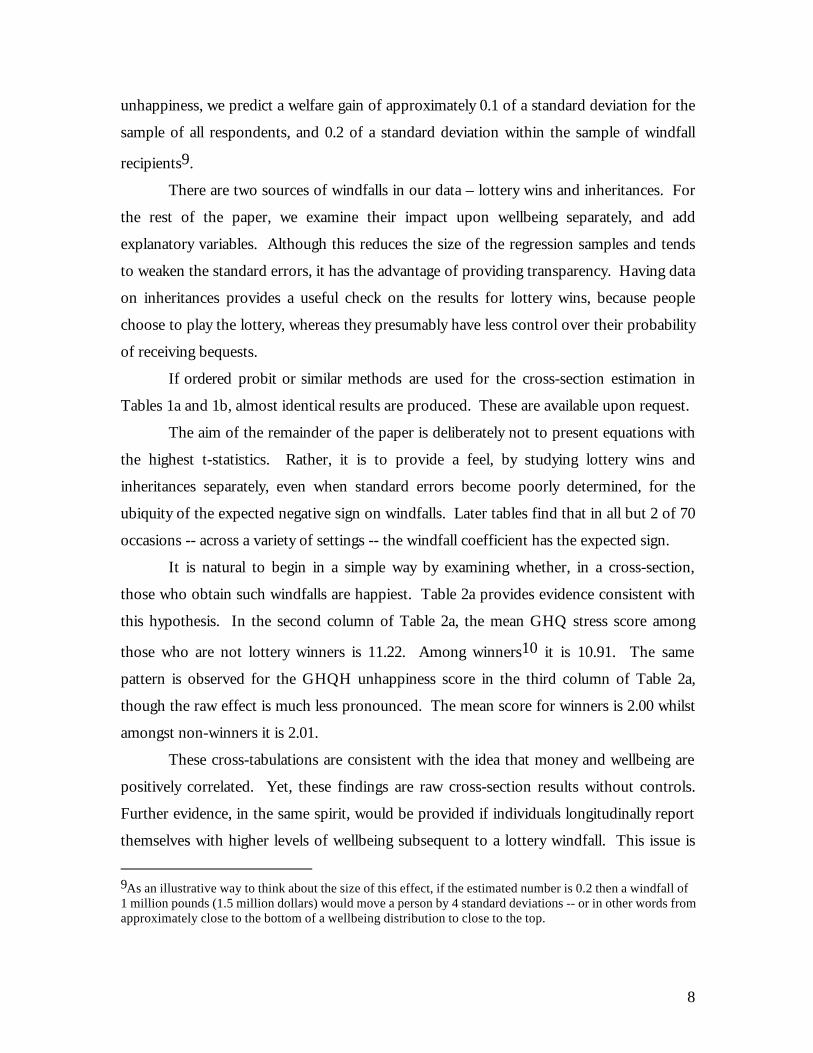
unhappiness, we predict a welfare gain of approximately 0.1 of a standard deviation for the

sample of all respondents, and 0.2 of a standard deviation within the sample of windfall

recipients9.

There are two sources of windfalls in our data – lottery wins and inheritances. For

the rest of the paper, we examine their impact upon wellbeing separately, and add

explanatory variables. Although this reduces the size of the regression samples and tends

to weaken the standard errors, it has the advantage of providing transparency. Having data

on inheritances provides a useful check on the results for lottery wins, because people

choose to play the lottery, whereas they presumably have less control over their probability

of receiving bequests.

If ordered probit or similar methods are used for the cross-section estimation in

Tables 1a and 1b, almost identical results are produced. These are available upon request.

The aim of the remainder of the paper is deliberately not to present equations with

the highest t-statistics. Rather, it is to provide a feel, by studying lottery wins and

inheritances separately, even when standard errors become poorly determined, for the

ubiquity of the expected negative sign on windfalls. Later tables find that in all but 2 of 70

occasions -- across a variety of settings -- the windfall coefficient has the expected sign.

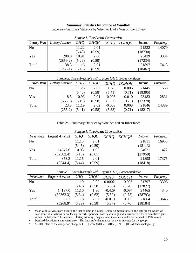
It is natural to begin in a simple way by examining whether, in a cross-section,

those who obtain such windfalls are happiest. Table 2a provides evidence consistent with

this hypothesis. In the second column of Table 2a, the mean GHQ stress score among

those who are not lottery winners is 11.22. Among winners10 it is 10.91. The same

pattern is observed for the GHQH unhappiness score in the third column of Table 2a,

though the raw effect is much less pronounced. The mean score for winners is 2.00 whilst

amongst non-winners it is 2.01.

These cross-tabulations are consistent with the idea that money and wellbeing are

positively correlated. Yet, these findings are raw cross-section results without controls.

Further evidence, in the same spirit, would be provided if individuals longitudinally report

themselves with higher levels of wellbeing subsequent to a lottery windfall. This issue is

9As an illustrative way to think about the size of this effect, if the estimated number is 0.2 then a windfall of1 million pounds (1.5 million dollars) would move a person by 4 standard deviations -- or in other words fromapproximately close to the bottom of a wellbeing distribution to close to the top.

9

investigated in the second panel of Table 2a (so-called Sample 2), and summary statistics

reported for those individuals where we observe the change in GHQ score. For this

sample, the mean lottery win, conditional on being a winner, is observed to be considerably

lower than that observed in the cross-section, respectively 118.5 and 200.0 pounds.

Investigation revealed this difference to be chiefly attributable to the dropping of large

lottery wins in the sample. Whether this selectivity reflects coincidence, or a more

systematic bias, is not here possible to ascertain. The direction of bias is not clear a priori

and will depend upon whether there are diminishing returns to wellbeing at very large

windfalls.

Despite these concerns, the mean GHQ and GHQH scores for both winners and

non-winners are remarkably similar to those observed previously. In the lower half of

Table 2a, column 2, the mean GHQ stress score among lottery winners is 10.93, compared

to 10.91 for the full sample (called Sample 1). Among non-winners it is 11.25, as opposed

to 11.22. Both samples appear to capture similar patterns of behaviour.

When the data are differenced, and changes over time in a person’s wellbeing

studied, we observe lottery winners to show on average increased levels of wellbeing (more

precisely a reduced lack of wellbeing). In the second half of Table 2a, individuals who

record a lottery win have an average decrease in GHQ mental stress of 0.096 points (see

the fourth column of Table 2a, Sample 2). Amongst non-winners, GHQ worsens on

average by approximately 0.020. For the GHQH unhappiness question the respective

figures for winners and non-winners are 0.010 and 0.006. The observed rise in wellbeing

subsequent to a lottery windfall appears pronounced when contrasted with the secular fall

in wellbeing for non-winners in this period.

Inheritances also work in the way that would be predicted. In Table 2b, the GHQ

mental stress scores of inheritors are on average better than the scores of those who do not

inherit any cash; they are 10.93 as opposed to 11.15 (see the second column of Table 2b,

Sample 1). For the GHQH unhappiness question, the mean response for inheritors is 1.95

in Table 2b, whilst for those who do not receive a bequest the measured level of

unhappiness is 2.01. Panel two of Table 2b, which uses the so-called Sample 2, restricts

attention to those individuals where we can observe the change in wellbeing over time.

10 We are unable to distinguish between those who do not gamble and those who do gamble but do notwin.

10

Both for those who inherit and those who do not, this (smaller) sample appears to be

representative of that observed for the pooled cross-section. Furthermore, this selection

does little to alter the tenor of the results.

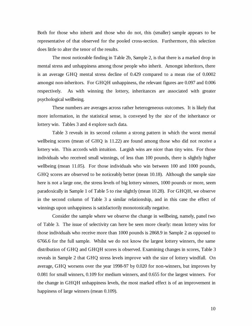
The most noticeable finding in Table 2b, Sample 2, is that there is a marked drop in

mental stress and unhappiness among those people who inherit. Amongst inheritors, there

is an average GHQ mental stress decline of 0.429 compared to a mean rise of 0.0002

amongst non-inheritors. For GHQH unhappiness, the relevant figures are 0.097 and 0.006

respectively. As with winning the lottery, inheritances are associated with greater

psychological wellbeing.

These numbers are averages across rather heterogeneous outcomes. It is likely that

more information, in the statistical sense, is conveyed by the size of the inheritance or

lottery win. Tables 3 and 4 explore such data.

Table 3 reveals in its second column a strong pattern in which the worst mental

wellbeing scores (mean of GHQ is 11.22) are found among those who did not receive a

lottery win. This accords with intuition. Largish wins are nicer than tiny wins. For those

individuals who received small winnings, of less than 100 pounds, there is slightly higher

wellbeing (mean 11.05). For those individuals who win between 100 and 1000 pounds,

GHQ scores are observed to be noticeably better (mean 10.18). Although the sample size

here is not a large one, the stress levels of big lottery winners, 1000 pounds or more, seem

paradoxically in Sample 1 of Table 5 to rise slightly (mean 10.28). For GHQH, we observe

in the second column of Table 3 a similar relationship, and in this case the effect of

winnings upon unhappiness is satisfactorily monotonically negative.

Consider the sample where we observe the change in wellbeing, namely, panel two

of Table 3. The issue of selectivity can here be seen more clearly: mean lottery wins for

those individuals who receive more than 1000 pounds is 2868.9 in Sample 2 as opposed to

6766.6 for the full sample. Whilst we do not know the largest lottery winners, the same

distribution of GHQ and GHQH scores is observed. Examining changes in scores, Table 3

reveals in Sample 2 that GHQ stress levels improve with the size of lottery windfall. On

average, GHQ worsens over the year 1998-97 by 0.020 for non-winners, but improves by

0.081 for small winners, 0.109 for medium winners, and 0.655 for the largest winners. For

the change in GHQH unhappiness levels, the most marked effect is of an improvement in

happiness of large winners (mean 0.109).

11

The same issue can be pursued for individuals who receive an inheritance. Table 4

reports the data. A consistent and intriguing cross-section pattern is revealed in both GHQ

and GHQH scores: a smallish inheritance of less than 2500 pounds is associated with the

highest level of wellbeing. An inheritance of between 2500 and 10,000 pounds on average

improves welfare relative to not receiving an inheritance but is associated with lower

wellbeing than the smallest level of inheritance. Individuals who receive the largest

inheritances, over 10,000 pounds, are however those with significantly worse cross-section

levels of wellbeing both for stress (GHQ) and unhappiness (GHQH). This is true in the

full sample and in the sample where we observe the change in wellbeing. Yet when we

instead examine the change in wellbeing in response to a bequest, both GHQ stress levels

and GHQH unhappiness levels are observed to have improved for all categories, relative to

a decline observed for non-inheritors. In the deltas, then, observed behaviour matches

intuition. The largest windfalls produce the greatest gains in GHQH wellbeing (column 5

of Table 4, Sample 2).

The summary statistics thus support the hypothesis that money is welfare

improving. Windfalls of cash are associated with higher levels of wellbeing. This is, in the

main, observed independent of how the data are cut, for both GHQ mental stress and

GHQH unhappiness scores, both when examining the level of wellbeing and its change

over time.

This evidence is fairly compelling. The recipients of windfalls have, on average,

higher levels of wellbeing. For such summary statistics to provide conclusive evidence,

however, would require the receipt and size of windfall to be randomly distributed across

individuals. Whilst windfalls may be unanticipated, this is unlikely always to be true. The

decision to gamble and the intensity of play are likely to be correlated with observed and

unobserved characteristics. Indeed early tables demonstrate a positive correlation between

lottery winnings and income. Furthermore, if happier people are more (or less) likely to

play, and thus win, the correlation between winnings and wellbeing could be due to some

subtle self-selection of players rather than any welfare-enhancing effects. Similarly,

inheritances may be positively associated with parental wealth, which is likely to be

correlated with recipient income (as seen in Tables 2 and 4). To investigate these issues in

more detail we turn to regression analysis.

12

Throughout the remainder of the paper we examine the robustness of the negative

sign on windfall gains.

Estimation strategy

The regression equation estimated is an empirical version of equation 1. Wellbeing is

assumed a function of the monetary windfall, personal characteristics (such as education,

gender, race, and region) and the time period. On occasion it is also examined whether

results are robust to the inclusion of family income as an explanatory variable. Wellbeing

for individual i, in time period t, is then expressed as:

(2) rit = wit'β + yit'δ + zit'γ + ε it i = 1,…,n

t = 1,…,T

where r is the dependent variable that captures individual wellbeing, w is the amount of

windfall (lottery win or inheritance), y is family income, z is a vector of individual

characteristics and time dummies, ε is the conformable error term with mean zero and

constant variance, and β , δ and γ the parameters to be estimated. The two measures of

wellbeing, the overall GHQ score (on a 0 to 36 scale) and the GHQH unhappiness

question (on a 0 to 3 scale), are approximated as linear and equations estimated by least

squares.11 Alternative specifications include a lagged dependent variable or instead adopt

the change in wellbeing as the dependent variable.

Lottery Wins

A simple regression-equation test of whether winning money improves wellbeing is

contained in Table 5. Here, and in all subsequent tables, panel A contains analysis of the

GHQ mental stress score, panel B the GHQH unhappiness score. For comparison, column

one of Table 5 reports the estimated effect of family income upon wellbeing. As expected,

richer people are happier. GHQ is estimated to improve by 0.117, and GHQH by 0.005,

for an increase in income of ten thousand pounds sterling. The controls here, and

throughout, are a quadratic in age, and dummies for gender, ethnic minority status,

educational qualifications, region, and year. This cross-section result is, however, likely to

confound various influences and cannot be presumed to capture causation.

11 This implicitly assumes responses are cardinal.

13

Columns two and three of Table 5 do a regression test of the hypothesis that lottery

winners are happier. Similarly to the sample statistics observed previously, wellbeing is

observed to be higher for those who receive winnings and it is increasing in the amount of

windfall. The monotonicity in column 3 is encouraging. Coefficient estimates are negative

but not usually independently well-determined. For people who win a small amount, such

as less than 100 pounds, there is only a negligible difference in wellbeing relative to non-

winners. This suggests that the pleasure associated with being a winner per se is largely

trivial, at least for the measures of wellbeing studied here, and should not greatly influence

results.

Column four of Table 5 instead enters the amount of winnings as the explanatory

variable. This gives a strong result. Both for GHQ mental stress and GHQH unhappiness,

the amount of winnings enters negatively -- thus improving wellbeing -- and is statistically

significant. A windfall of 10,000 pounds improves GHQ mental wellbeing by 0.686 with a

t-statistic above 6 and the GHQH unhappiness score by 0.032 with a t-statistic of 2.01.

These effects are of a magnitude approximately 6 times as large as those estimated for

income; it is not easy to know why.

The impact of a 50,000 pounds lottery windfall is estimated from Table 5 to

improve GHQ mental stress by 3.43 points or over 0.6 of a standard deviation. The

improvement in GHQH is slightly less marked at 0.16, but still constitutes approximately

0.3 of a standard deviation. Nevertheless, if ‘gamblers’ in general have high (low) levels of

wellbeing independent of any monetary gain, we shall overestimate (underestimate) the

effects of a windfall upon welfare. If gambling behaviour is characterised by such

selection, then coefficient estimates may be different when we restrict attention to a

sample of winners only. All individuals are then gamblers and they are also likely to be the

more intensive players. In this case, selection bias should be reduced. Column five of

Table 5 checks this and reveals that both for GHQ and GHQH the estimated effects of

winnings are similar, for the sample of all individuals and the sample of winners. This is

reassuring and suggests that the impact of winnings upon wellbeing is broadly orthogonal

to the selection of gamblers.12

12 Ideally one would wish to instrument winnings by a variable correlated with play but uncorrelated withwellbeing. However, as we analyse the effect of the amount won, a large degree of random variation is

14

Walker (1998) and Farrell and Walker (1999) provide some evidence that lottery

expenditure is a form of inferior good, that is, increasing in income but at a declining rate.

Our amount-won variable may then capture the effect of income and be prone to similar

problems of status and selection. Table 6 examines whether the effect of a lottery windfall

is robust to the inclusion of a control for income. Column one restates the basic result.

Column two of Table 6 adds family income as an explanatory variable. For both the GHQ

mental stress and the GHQH unhappiness measures of wellbeing, the estimated coefficient

upon the amount won is essentially unaltered – indicating that the psychological benefits of

winnings occur largely independently of income.

There is potential for non-linearity. This is checked in column three of Table 6,

where quadratics in the amount of winnings and income are examined. The first and

second-order terms for the amount won enter with the expected signs consistent with

diminishing returns but are not statistically significantly different from zero – neither for

stress (GHQ) or reported feelings of unhappiness (GHQH).

An alternative approach to the self-selection of gamblers is followed in Table 7.

This assumes the effects of selection are stable over time, and then scrutinises the change

in wellbeing associated with a windfall.

As seen previously, the sample of individuals where such data are observed omits

some of the largest windfalls. This has the effect of increasing the magnitude of the

estimated effect of winnings upon mental stress (GHQ) and reducing the estimated effect

upon unhappiness (GHQH) and in both cases reduces the precision of estimates.

Nevertheless, when a lagged dependent variable is included in column three of Table 7, the

effect is to increase the estimated gain in wellbeing subsequent to a lottery win. In

contrast, the coefficient upon income is driven towards zero and is no longer well-

determined.

In column three of Table 7 a control for previous gambling behaviour is added –

whether the individual received a lottery windfall in 199513. Again the estimated

coefficient upon amount won is more pronounced whilst the income parameter is

unaffected. Furthermore, previous gambling exerts a positive though not well-determined

introduced subsequent to participation. This is why this variable is of particular interest; yet as a result, novariable was available that identified the amount won separately from wellbeing.13 The amount won is not known.

15

effect upon both GHQ mental stress and GHQH unhappiness scores.14 This evidence

suggests that any differences in wellbeing levels between gamblers and non-gamblers do

not crucially shape results.

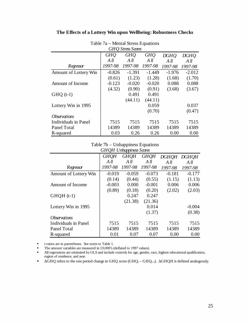
A similar conclusion is reached when we examine the change in wellbeing scores

over time in columns four and five of Table 7. For GHQ mental stress scores, a windfall

of 10,000 pounds is predicted to improve wellbeing, relative to the previous year, by 1.976.

This effect is statistically significant only at the 10 percent level. By comparison, in

column one of Table 7, where the dependent variable is the level of GHQ the predicted

improvement in wellbeing is 0.826. Similar results are observed for GHQH unhappiness,

although coefficient estimates are again not well-determined. Interestingly, high-income

individuals are observed in Table 7’s column five to have experienced, on average, a

secular decline in wellbeing levels over this period, both for GHQ and GHQH.

Hence, whilst, due to the characteristics of the sample, care must be taken in

interpretation, results seem robust to the inclusion of a lagged dependent variable, to

controlling for previous gambling success, and to examining the change in wellbeing over

time. If anything, such checks magnify the improvement in wellbeing from a lottery

windfall.

Inheritances

A potential difficulty with the examination of lottery wins is that the act of gambling, and

winning, may bring pleasure independent of monetary gain. Table 8 therefore explores the

impact upon wellbeing of receiving an inheritance. This event is likely to occur with the

death of a close friend or relative and hence, in contrast, often be associated with

reductions in wellbeing.

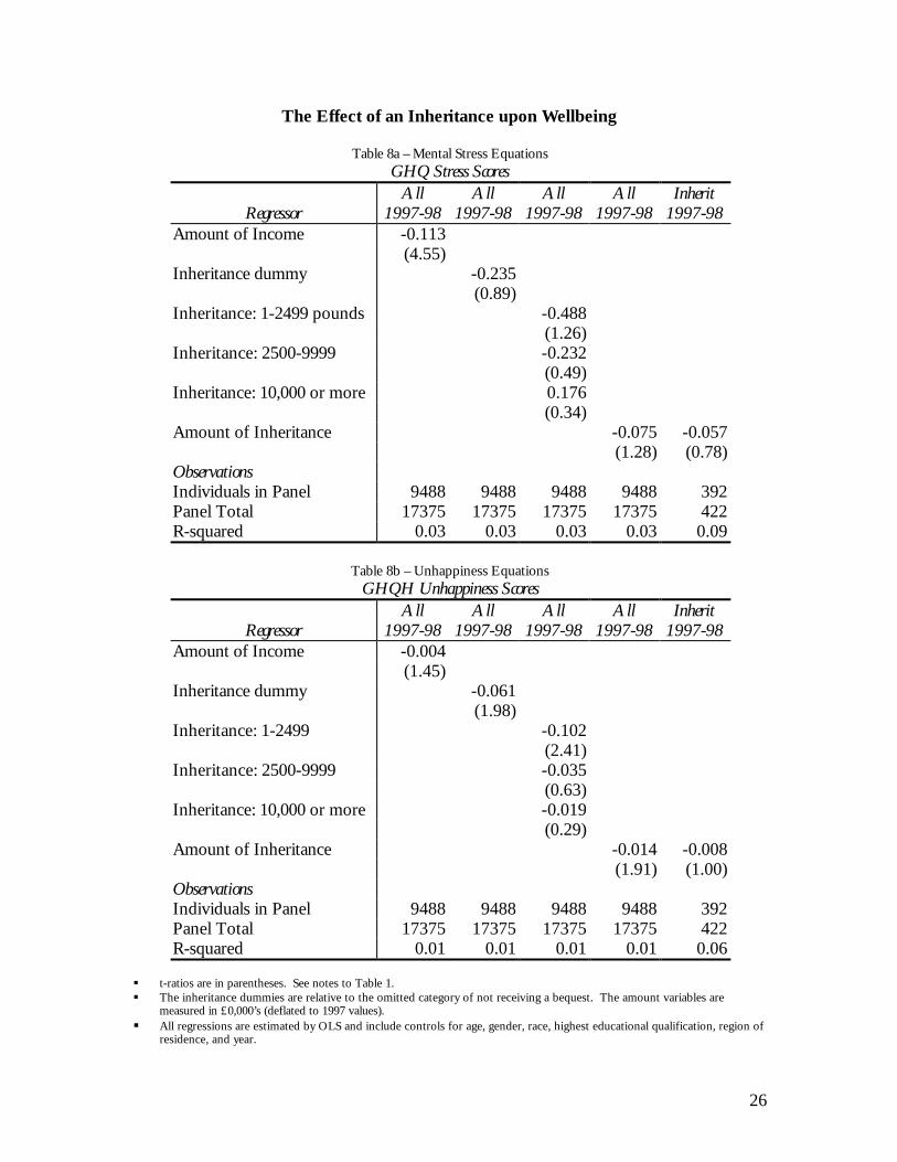
Column one of Table 8 estimates the effect of income upon wellbeing for this

sample. Results are close to those in column one of Table 5. Table 8’s column two

examines a simple test of whether a windfall increases happiness. Receiving a bequest is

found to improve wellbeing for both GHQ mental stress and GHQH unhappiness scores.

For GHQ the estimated coefficient is -0.235, for GHQH -0.061, though only the latter

effect is statistically robust. Column three extends this analysis by instead entering

14 This result holds if lottery winnings in the current year are omitted.

16

dummies for the amount of inheritance. For both measures of wellbeing it is

predominantly small inheritances, of less than 2500 pounds, that are observed to reduce

mental stress and unhappiness. The effect upon GHQ is estimated at -0.488. For GHQH

the parameter estimate is -0.102. Again only the latter effect is statistically significant.

Medium sized bequests are observed to improve wellbeing, whilst the largest inheritances

are estimated to increase GHQ mental stress, though to reduce GHQH unhappiness.

Column four of Table 8 examines the effect of the amount of inheritance, in tens of

thousands of pounds, upon wellbeing. Both GHQ and GHQH scores are shown to be

improving in the size of the bequest, despite the non-linearity observed above. A bequest

of 10,000 pounds is predicted to improve the GHQ mental health score by 0.075 points

and the GHQH unhappiness score by 0.014 points. When analysis is conditional upon

only those individuals who do inherit, in column five of Table 8, both GHQ and GHQH

coefficients are attenuated and are less precisely estimated but remain negative.

McGarry (1999) examines data on intended bequests and finds that the major

determinant of the size of bequest is parental wealth. A significant role is, though, found

also for the closeness of family relations.

With respect to the data studied here, recipients of the smallest category of

inheritance (less than 2500 pounds) may include grandchildren rather than children and

individuals with weaker parental links. They may then be more distant from the deceased

benefactor and thus likely to suffer less distress. As the amount of inheritance increases,

we potentially observe individuals with closer ties to the deceased. Also, larger

inheritances may be in the form of property or other assets, which themselves may induce

greater levels of stress in possibly disposing of. The improvement in wellbeing observed

for small inheritances may be being offset for larger bequests by the mental stress

associated with bereavement.

Alternatively, those who inherit are themselves likely to be more affluent, due to

linkages in family wealth, potentially with higher levels of wellbeing. Yet for such a

mechanism to explain the behaviour observed here would require this effect to be felt for

small inheritances but not for large. Such a relation seems doubtful, especially as the age,

gender, race, education and region of the recipient are held constant.

Table 9 seeks to investigate these issues. It uses the sample of individuals where

past (i.e. lagged levels of) GHQ and GHQH data are available. Column one replicates the

17

result for column four of Table 8. Parameter estimates are found to be similar, though less

well determined. In column two of Table 9, family income is added as an explanatory

variable. If the observed effect of the size of inheritance upon wellbeing reflects the

wealth of inheritors, then the addition of this variable should drive the estimated

coefficient towards zero. In fact, the estimated relationship between wellbeing and

bequests seems to be orthogonal to the inclusion of an income control. Furthermore, when

we add a lagged dependent variable or instead examine the change in wellbeing15, in

columns three and four of Table 9 respectively, the estimated beneficial effect of a bequest

increases. Thus the results do not depend upon the wealth of inheritors.

Any gains in wellbeing associated with an inheritance are potentially contaminated

by distress associated with the death of a close relative. The results so far may then form a

lower bound upon the true effect. Assuming stress levels are liable to be high both pre-

and post-bereavement, it seems natural to examine how wellbeing changes over time in

response to an inheritance. Columns one and two of Table 10 indicate an improvement in

both GHQ mental health scores and GHQH unhappiness scores that itself is increasing in

the size of the bequest. This is true both within the sample of all individuals and the

sample restricted to inheritors only. A 50,000 pounds inheritance is then predicted to

produce an improvement in GHQ mental stress of 0.99 and GHQH unhappiness of 0.15,

both of which are approximately 0.2 of a standard deviation.

The results may reflect heightened distress pre-bereavement and a subsequent

return to ‘normal’ wellbeing levels. If so, we spuriously overestimate the effect of a

windfall. If the bequest is anticipated, consumption patterns may change in advance,

improving welfare, and so we underestimate the true gain in wellbeing. Hence we next

examine the change in wellbeing over longer time periods, namely, two-year and three-year

gaps. Columns three to six of Table 10 show that the results are robust to such

considerations; indeed the gains in wellbeing from an inheritance appear to be amplified. A

bequest of 10,000 pounds improves the GHQ mental stress score by 0.520 and the GHQH

unhappiness scores by 0.083 – compared to the wellbeing levels that prevailed three years

prior. The latter effect is found to be statistically significant at normal confidence levels.

15 This will capture the effect of selectivity if it remains stable over time.

18

5. Conclusions

Economists assume, without detailed evidence, that a person who becomes richer becomes

happier. This paper shows that what is arguably the central tenet of economics is

supported by the data.

While it is known from recent cross-sectional work that reported happiness is

positively correlated with income, that is not a persuasive reason to believe that more

money leads to greater wellbeing. Cross-section patterns are at best suggestive because

their causal implications are hard to interpret. Constructing a compelling test is difficult

because of the stringent requirements of an ideal data set. Our approach seems to have

three advantages. First, we follow a group of individuals longitudinally, and thus can

measure the same person’s wellbeing and income level at different points in time. Second,

the data set provides information on financial windfalls (inheritances and lottery wins).

These are probably as close as can be achieved to randomly occurring events in which

some individuals have money showered upon them while others, in a control group, do not.

Third, information is available on two ways to measure wellbeing: mental stress using a

standard psychological health measure, and happiness using a simple four-point question.

We find that, as theory predicts, a windfall of money in year t is followed by lower

mental stress and higher reported happiness16. As a conservative estimate, a windfall of

50,000 pounds (75,000 US dollars) improves mental wellbeing by between 0.1 and 0.3

standard deviations.

16 Because we have data on both windfalls and wellbeing only for two years right at the end of our sample,it is not possible to assess whether people adapt psychologically to a windfall (perhaps returning eventuallyto some baseline happiness level). But the longitudinal data collection is continuing, so eventually it shouldbe possible to address this question.

19

The Effects of Windfalls upon Two Measures of Wellbeing in a Panel

Table 1a – Mental Stress EquationsGHQ Stress Scores

RegressorAll

GHQAll

GHQWindfallGHQ

All∆GHQ

All∆GHQ

Windfall∆GHQ

Windfall dummy -0.299 -0.156(2.83) (1.64)

Ln(Windfall amount) -0.054 -0.103 -0.034 -0.101(3.45) (2.26) (2.31) (2.13)

ObservationsIndividuals in Panel 9588 9588 2932 8620 8620 2722Panel Total 17556 17556 3737 16075 16075 3478

Mean GHQ stress score 11.14 11.14 10.90 11.16 11.16 10.93(5.44) (5.44) (5.28) (5.43) (5.43) (5.27)

Mean windfall amount in pounds 388.7 388.7 1825.9 376.0 376.0 1737.6[1 pound equals 1.5 US dollars] (5655.3) (5655.3) (12151.5) (5344.5) (5344.5) (12387.8)

Table 1b – Unhappiness EquationsGHQH Unhappiness Scores

RegressorAll

GHQHAll

GHQHWindfallGHQH

All∆GHQH

All∆GHQH

Windfall∆GHQH

Windfall dummy -0.014 -0.026(1.24) (2.03)

Ln(Windfall amount) -0.003 -0.011 -0.005 -0.013(1.86) (2.05) (2.59) (2.02)

ObservationsIndividuals in Panel 9588 9588 2932 8696 8696 2737Panel Total 17556 17556 3737 16201 16201 3499

Mean GHQH unhappiness score 2.01 2.01 2.00 2.01 2.01 2.00(0.59) (0.59) (0.59) (0.59) (0.59) (0.59)

Mean windfall amount in pounds 388.7 388.7 1825.9 376.0 376.0 1737.6[1 pounds equals 1.5 US dollars] (5655.3) (5655.3) (12151.5) (5344.5) (5344.5) (12387.8)

§ t-ratios are in parentheses. Standard errors are robust to arbitrary heteroscedasticity and the repeat sampling ofindividuals. All estimates are from least squares bivariate regressions. Data are for 1997 and 1998.

§ GHQ is a measure of mental stress on a 36-point scale. GHQH is a measure of unhappiness on a 4-point scale.§ ‘All’ refers to the whole sample. The heading ‘Windfall’ refers to the sub-sample of those people who receive a non-

zero windfall. Windfalls refer to cumulative gains, from lottery winnings plus inheritances, within the last year. Theyare deflated to 1997 values.

§ The log of windfall corrects the zero-windfall terms by adding a small constant (0.1).§ The first three columns are cross-sections. The second three columns are differences.§ Where sample means are reported, standard deviations are in parentheses.

20

Summary Statistics by Source of WindfallTable 2a – Summary Statistics by Whether Had a Win on the Lottery

Sample 1: The Pooled Cross-sectionLottery Win Lottery Amount GHQ GHQH ∆GHQ ∆GHQH Income FrequencyNo 11.22

(5.48)2.01

(0.59)21532

(18730)14079

Yes 200.0(2859.2)

10.91(5.29)

2.00(0.59)

23439(17234)

3334

Total 38.3(1253.4)

11.16(5.45)

2.01(0.59)

21897(18467)

17413

Sample 2: The sub-sample with Lagged GHQ Scores availableLottery Win Lottery Amount GHQ GHQH ∆GHQ ∆GHQH Income FrequencyNo 11.25

(5.46)2.02

(0.58)0.020(5.41)

0.006(0.71)

21445(18395)

11558

Yes 118.5(565.6)

10.93(5.19)

2.01(0.58)

-0.096(5.27)

-0.010(0.70)

23483(17378)

2831

Total 23.3(255.2)

11.19(5.41)

2.02(0.58)

-0.003(5.38)

0.003(0.71)

21846(18217)

14389

Table 2b - Summary Statistics by Whether had an Inheritance

Sample 1: The Pooled Cross-sectionInheritance Bequest Amount GHQ GHQH ∆GHQ ∆GHQH Income FrequencyNo 11.15

(5.45)2.01

(0.59)21811

(18113)16953

Yes 14547.6(32582.4)

10.93(5.16)

1.95(0.61)

24621(27959)

422

Total 353.3(5544.4)

11.15(5.44)

2.01(0.59)

21898(18418)

17375

Sample 2: The sub-sample with Lagged GHQ Scores availableInheritance Bequest Amount GHQ GHQH ∆GHQ ∆GHQH Income FrequencyNo 11.19

(5.40)2.02

(0.58)0.0002(5.36)

0.006(0.70)

21797(17827)

13306

Yes 14137.0(30362.3)

11.10(5.34)

1.96(0.62)

-0.429(5.59)

-0.097(0.78)

24465(28793)

340

Total 352.2(5268.9)

11.18(5.39)

2.02(0.58)

-0.010(5.37)

0.003(0.70)

21864(18184)

13646

§ Mean windfall values are given in the first column in pounds. Sample 2 means those in the data set for whom wehave some observations on wellbeing for earlier periods. Lottery winnings and inheritances refer to cumulative gainswithin the last year. The amount of lottery winnings, bequests and income variables are deflated to 1997 values.

§ Standard deviations are in parentheses. The ‘Income’ column gives the mean incomes for the groups.§ ∆GHQ refers to the one period change in GHQ score (GHQt – GHQt-1). ∆GHQH is defined analogously.

21

Summary Statistics by Amount of Windfall

Table 3 – Summary Statistics by Amount of Win on Lottery

Sample 1: The Pooled Cross-sectionLottery Win Lottery Amount GHQ GHQH ∆GHQ ∆GHQH Income FrequencyNo 11.22

(5.48)2.01

(0.59)21532

(18730)14079

1-99 28.6(24.1)

11.05(5.34)

2.01(0.59)

23098(16684)

2769

100-999 256.6(195.4)

10.18(4.98)

1.98(0.56)

23921(17278)

497

1000 plus 6766.6(19009.5)

10.28(4.67)

1.94(0.57)

33776(30829)

68

Total 38.30(1253.4)

11.16(5.45)

2.01(0.59)

21897(18467)

17413

Sample 2: The sub-sample with Lagged GHQ Scores availableLottery Win Lottery Amount GHQ GHQH ∆GHQ ∆GHQH Income FrequencyNo 11.25

(5.46)2.02

(0.58)0.020(5.41)

0.006(0.71)

21445(18395)

11558

1-99 28.9(23.9)

11.07(5.22)

2.02(0.58)

-0.081(5.28)

-0.011(0.71)

23073(16667)

2353

100-999 259.7(200.2)

10.24(5.02)

1.98(0.57)

-0.109(5.30)

0.009(0.66)

24156(17707)

423

1000 plus 2868.9(2865.8)

10.31(4.53)

1.98(0.59)

-0.655(4.25)

-0.109(0.66)

35878(33319)

55

Total 23.3(255.2)

11.19(5.41)

2.02(0.58)

-0.003(5.38)

0.003(0.71)

21846(18217)

14389

§ Lottery winnings and inheritances refer to cumulative gains within the last year. The amount of lottery winnings,bequests and income variables are deflated to 1997 values.

§ Standard deviations are in parentheses.§ ∆GHQ refers to the one period change in GHQ score (GHQt – GHQt-1). ∆GHQH is defined analogously.

22

Table 4 – Summary Statistics by Amount of Inheritance

Sample 1: The Pooled Cross-sectionInheritance Bequest Amount GHQ GHQH ∆GHQ ∆GHQH Income FrequencyNo 11.15

(5.45)2.01

(0.59)21811

(18113)16953

1-2499 881.7(629.3)

10.58(5.04)

1.89(0.56)

24269(19974)

189

2500-9999

5351.7(2150.1)

10.95(5.19)

1.97(0.61)

23270(14219)

118

10,000 + 46442.8(49917.4)

11.50(5.34)

2.02(0.68)

26588(44894)

115

Total 353.3(5544.4)

11.15(5.44)

2.01(0.59)

21880(18418)

17375

Sample 2: The sub-sample with Lagged GHQ Scores availableInheritance Bequest Amount GHQ GHQH ∆GHQ ∆GHQH Income FrequencyNo 11.19

(5.40)2.02

(0.58)0.0002(5.36)

0.0061(0.70)

21797(17827)

13306

1-2499 908.4(641.5)

10.76(5.20)

1.90(0.58)

-0.2800(5.42)

-0.0933(0.74)

23489(19709)

150

2500-9999

5477.4(2177.6)

11.04(5.25)

1.99(0.61)

-0.8242(5.43)

-0.0769(0.67)

24366(14723)

91

10,000 + 42140.3(45324.0)

11.68(5.62)

2.04(0.68)

-0.2929(6.00)

-0.1212(0.91)

26033(45544)

99

Total 352.2(5268.9)

11.18(5.39)

2.02(0.58)

-0.0105(5.37)

0.0035(0.70)

21864(18184)

13646

§ Lottery winnings and inheritances refer to cumulative gains within the last year. The amount of lottery winnings,bequests and income variables are deflated to 1997 values.

§ Standard deviations are in parentheses.§ ∆GHQ refers to the one period change in GHQ score (GHQt – GHQt-1). ∆GHQH is defined analogously.

23

The Effect of a Lottery Win upon Wellbeing


RegressorAll

1997-98All

1997-98All

1997-98All

1997-98Win

1997-98Amount of Income -0.117

(4.72)Lottery Win -0.199

(1.81)Lottery Win: 1-99 pounds -0.077

(0.65)Lottery Win: 100-999 -0.796

(3.36)Lottery Win: 1000 or more -0.825

(1.37)Amount of Lottery Win -0.686 -0.666

(6.26) (5.36)ObservationsIndividuals in Panel 9493 9493 9493 9493 2607Panel Total 17413 17413 17413 17413 3334R-squared 0.03 0.03 0.03 0.03 0.03


Regressor All1997-98

All1997-98

All1997-98

All1997-98

Win1997-98

Amount of Income -0.005(1.74)

Lottery Win -0.005(0.45)

Lottery Win: 1-99 pounds 0.000(0.01)

Lottery Win: 100-999 -0.026(1.00)

Lottery Win: 1000 or more -0.078(1.14)

Amount of Lottery Win -0.032 -0.031(2.01) (1.74)

ObservationsIndividuals in Panel 9493 9493 9493 9493 2607Panel Total 17413 17413 17413 17413 3334R-squared 0.01 0.01 0.01 0.01 0.02

§ t-ratios are in parentheses. See notes to Table 1.§ The lottery win dummies are relative to the omitted category of zero winnings. The amount variables are measured

in £0,000’s (deflated to 1997 values).§ All regressions are estimated by OLS and include controls for age, gender, race, highest educational qualification,

region of residence, and year.

24

The Effect of a Lottery Win upon Wellbeing: Non-linear Income Effects


RegressorAll

1997-98All

1997-98All

1997-98Amount of Lottery Win -0.686 -0.664 -1.510

(6.26) (6.35) (1.16)(Amount of Lottery Win)2/100 0.917

(0.67)Amount of Income -0.117 -0.172

(4.69) (4.86)(Amount of Income)2/100 0.041

(2.86)ObservationsIndividuals in Panel 9493 9493 9493Panel Total 17413 17413 17413R-squared 0.03 0.03 0.03


RegressorAll

1997-98All

1997-98All

1997-98Amount of Lottery Win -0.032 -0.031 -0.142

(2.01) (1.98) (0.96)(Amount of Lottery Win)2/100 0.121

(0.78)Amount of Income -0.005 -0.006

(1.73) (1.68)(Amount of Income)2/100 0.001

(1.08)ObservationsIndividuals in Panel 9493 9493 9493Panel Total 17413 17413 17413R-squared 0.01 0.01 0.01

§ t-ratios are in parentheses. See notes to Table 1.§ The amount variables are measured in £0,000’s (deflated to 1997 values).§ All regressions are estimated by OLS and include controls for age, gender, race, highest educational qualification,

region of residence, and year.

25

The Effects of a Lottery Win upon Wellbeing: Robustness Checks


Regressor

GHQAll

1997-98

GHQAll

1997-98

GHQAll

1997-98

∆GHQAll

1997-98

∆GHQAll

1997-98Amount of Lottery Win -0.826 -1.391 -1.449 -1.976 -2.012

(0.61) (1.23) (1.28) (1.68) (1.70)Amount of Income -0.123 -0.020 -0.020 0.088 0.088

(4.32) (0.90) (0.91) (3.68) (3.67)GHQ (t-1) 0.491 0.491

(44.11) (44.11)Lottery Win in 1995 0.059 0.037



Regressor

GHQHAll

1997-98

GHQHAll

1997-98

GHQHAll

1997-98

∆GHQHAll

1997-98

∆GHQHAll

1997-98Amount of Lottery Win -0.019 -0.059 -0.073 -0.181 -0.177

(0.14) (0.44) (0.55) (1.15) (1.13)Amount of Income -0.003 0.000 -0.001 0.006 0.006

(0.89) (0.18) (0.20) (2.02) (2.03)GHQH (t-1) 0.247 0.247

(21.38) (21.36)Lottery Win in 1995 0.014 -0.004



region of residence, and year.§ ∆GHQ refers to the one period change in GHQ score (GHQt – GHQt-1). ∆GHQH is defined analogously.

26

The Effect of an Inheritance upon Wellbeing


RegressorAll

1997-98All

1997-98All

1997-98All

1997-98Inherit


(4.55)Inheritance dummy -0.235

(0.89)Inheritance: 1-2499 pounds -0.488

(1.26)Inheritance: 2500-9999 -0.232

(0.49)Inheritance: 10,000 or more 0.176

(0.34)Amount of Inheritance -0.075 -0.057



RegressorAll

1997-98All

1997-98All

1997-98All

1997-98Inherit


(1.45)Inheritance dummy -0.061

(1.98)Inheritance: 1-2499 -0.102

(2.41)Inheritance: 2500-9999 -0.035

(0.63)Inheritance: 10,000 or more -0.019

(0.29)Amount of Inheritance -0.014 -0.008


§ t-ratios are in parentheses. See notes to Table 1.§ The inheritance dummies are relative to the omitted category of not receiving a bequest. The amount variables are

measured in £0,000’s (deflated to 1997 values).§ All regressions are estimated by OLS and include controls for age, gender, race, highest educational qualification, region of

residence, and year.

27

The Effect of an Inheritance upon Wellbeing: Robustness Checks


Regressor

GHQAll

1997-98

GHQAll

1997-98

GHQAll

1997-98

∆GHQAll

1997-98

∆GHQAll

1997-98Amount of Inheritance -0.075 -0.078 -0.136 -0.198 -0.196

(0.96) (0.99) (1.16) (1.11) (1.10)Amount of Income -0.113 -0.014 0.089

(3.90) (0.62) (3.65)GHQ (t-1) 0.492

(43.54)ObservationsIndividuals in Panel 7262 7262 7262 7262 7262Panel Total 13646 13646 13646 13646 13646R-squared 0.03 0.03 0.26 0.00 0.00


Regressor

GHQHAll

1997-98

GHQHAll

1997-98

GHQHAll

1997-98

∆GHQHAll

1997-98

∆GHQHAll

1997-98Amount of Inheritance -0.009 -0.009 -0.014 -0.030 -0.030

(0.96) (0.96) (1.18) (1.29) (1.28)Amount of Income -0.001 0.001 0.007

(0.39) (0.32) (2.27)GHQH (t-1) 0.248

(21.07)ObservationsIndividuals in Panel 7262 7262 7262 7262 7262Panel Total 13646 13646 13646 13646 13646R-squared 0.01 0.01 0.07 0.00 0.00


region of residence, and year.§ ∆GHQ refers to the one period change in GHQ score (GHQt – GHQt-1).

28

The Effect of an Inheritance upon Wellbeing: First Differences


Regressor

∆GHQAll

1997-98

∆GHQInherit

1997-98

∆2GHQAll

1997-98

∆2GHQInherit

1997-98

∆3GHQAll

1997-98

∆3GHQInherit

1997-98Amount of Inheritance -0.196 -0.235 -0.363 -0.450 -0.520 -0.683

(1.10) (1.07) (1.23) (1.26) (1.26) (1.41)Amount of Income 0.089 -0.031 0.087 -0.251 0.054 -0.605

(3.65) (0.37) (2.29) (1.55) (0.84) (2.13)ObservationsIndividuals in Panel 7262 316 7262 316 7262 316Panel Total 13646 340 13646 340 13646 340R-squared 0.00 0.06 0.00 0.06 0.00 0.08


Regressor

∆GHQHAll

1997-98

∆GHQHInherit

1997-98

∆2GHQHAll

1997-98

∆2GHQHInherit

1997-98

∆3GHQHAll

1997-98

∆3GHQHInherit

1997-98Amount of Inheritance -0.030 -0.031 -0.060 -0.072 -0.083 -0.108

(1.28) (1.07) (1.83) (1.73) (2.15) (2.21)Amount of Income 0.007 -0.002 0.008 -0.017 0.007 -0.036

(2.27) (0.20) (1.61) (0.82) (0.79) (0.93)ObservationsIndividuals in Panel 7262 316 7262 316 7262 316Panel Total 13646 340 13646 340 13646 340R-squared 0.00 0.06 0.00 0.07 0.00 0.08


region of residence, and year.§ ∆GHQ refers to the one period change in GHQ score (GHQt – GHQt-1). ∆2GHQ is the two period change in GHQ

score (GHQt – GHQt-2). ∆3GHQ is the three period change in GHQ score (GHQt – GHQt-3). Terms are definedsimilarly for GHQH.

29

References

Andrews, F.M. “Stability and change in levels and structure of subjective wellbeing: USA1972 and 1988.” Social Indicators Research 25 (1991): 1-30.

Argyle, M. The Psychology of Happiness. London: Routledge, 1989.Blanchflower, D.G., Oswald, A.J. and P.B. Warr. “Wellbeing over time in Britain and the

USA.” : LSE, 1993.Blanchflower, D.G. and A.J. Oswald. “The rising wellbeing of the young.” In Youth

Employment and Joblessness in Advanced Countries, edited by D.G. Blanchflower andR.B. Freeman: University of Chicago Press and NBER, 1999.

Blanchflower, D.G. and A.J. Oswald. “What makes an entrepreneur?” Journal of LaborEconomics 16 (1998): 26-60.

Blanchflower, D.G. and R.B. Freeman. “The legacy of Communist labor relations.”Industrial and Labor Relations Review 50 (1997): 438-459.

Bodkin, R. “Windfall income and consumption.” American Economic Review 49 (1959): 602-614.

Brickman, P., Coates, D. and R. Janoff-Bulman “Lottery winners and accident victims: Ishappiness relative?” Journal of Personality and Social Psychology 36 (1978): 917-927.

Campbell, A. The Sense of Wellbeing in America . New York: McGraw Hill, 1981.Chen, P.Y. and P.E. Spector. “Negative affectivity as the underlying cause of correlations

between stressors and strains.” Journal of Applied Psychology 7 (1991): 398-407.Clark, A.E. “Job satisfaction in Britain.” British Journal of Industrial Relations 34 (1996): 189-

217.Clark, A.E. “Wellbeing in panels.” : University of Orleans, 1999.Clark, A.E. and A.J. Oswald. “Satisfaction and comparison income.” Journal of Public

Economics 61 (1996): 359-381.Clark, A.E. and A.J. Oswald. “Unhappiness and unemployment.” Economic Journal 104

(1994): 648-659.Cochrane, R. “Marriage and madness.” Psychology Review 3 (1996): 2-5.Cooper, B. and C. Garcia-Penalosa. “Status effects and negative utility growth.” : Nuffield

College, Oxford., 1999.Cox, D. “Motives for private income transfers.” Journal of Political Economy 95 (1987): 508-

546.Di Tella, R., MacCulloch, R. and A.J. Oswald. “The macroeconomics of happiness.” :

Harvard Business School, 1998.Di Tella, R., MacCulloch, R. and A.J. Oswald. “Preferences over inflation and

unemployment: Evidence from surveys of happiness.” American Economic Reviewforthcoming (March 2001).

Di Tella, R. and R. MacCulloch. “Partisan social happiness.” : Harvard Business School.,1999.

Diener, E. “Subjective wellbeing.” Psychological Bulletin 95 (1984): 542-575.Diener, E. and R. Biswas-Diener. “ Will money increase subjective wellbeing? A literature

review and guide to needed research.”, 2000, mimeo, University of Illinois.Diener, E., Suh, E.M., Lucas, R.E., and H.L. Smith. “Subjective wellbeing: Three decades

of progress.” Psychological Bulletin 125 (1999): 276-303.Diener, E., Gohm, C.L., Suh, E. and S. Oishi. “Similarity of the relations between marital

status and subjective wellbeing across cultures.” . Urbana: Psychology Department,University of Illinois, undated.

30

Douthitt, R.A., MacDonald, M. and R. Mullis. “The relationship between measures ofsubjective and economic wellbeing: A new look.” Social Indicators Research 26(1992): 407-422.

Duesenberry, J.S. Income, Saving and the Theory of Consumer Behavior. Cambridge, Mass.:Harvard University Press, 1949.

Easterlin, R.A. “Does economic growth improve the human lot? Some empiricalevidence.” In Nations and Households in Economic Growth: Essays in Honour of MosesAbramowitz, edited by P.A. David and M.W. Reder. New York and London.:Academic Press, 1974.

Easterlin, R.A. “Will raising the incomes of all increase the happiness of all?” Journal ofEconomic Behavior and Organization 27 (1995): 35-47.

Farrell, L. and I. Walker. “The welfare effects of lotto: Evidence from the UK.” Journal ofPublic Economics 72 (1999): 99-120.

Fordyce, M.W. “The psychap inventory: A multi-scale test to measure happiness and itsconcomitants.” Social Indicators Research 18 (1985): 1-33.

Fox, C.R. and D. Kahneman. “Correlations, causes and heuristics in surveys of lifesatisfaction.” Social Indicators Research 27 (1992): 221-234.

Frank, R. H. Choosing the Right Pond. New York: Oxford University Press, 1985.Frank, R.H. “The frame of reference as a public good.” Economic Journal 107 (1997): 1832-

1847.Frank, R.H. Luxury Fever. Oxford: Oxford University Press, 1999.Frey, B.S. and F. Schneider. “An empirical study of politico-economic interaction in the

United States.” Review of Economics and Statistics 60 (1978): 174-183.Frey, B.S. and A. Stutzer. “Happiness, economy and institutions.” Economic Journal 110

(2000): 918-938Frey, B.S. and A. Stutzer. “Measuring preferences by subjective wellbeing.” : working

paper, University of Zurich, 1998.Frisch, M.B, Cornell, J., Villanueva, M., and P.J. Retzlaff. “Clinical validation of the quality

of life inventory: A measure of life satisfaction for use in treatment planning andoutcome assessment.” Pyschological Assessment 4 (1992): 92-101.

Gallie, D., White, M., Cheng, Y. and M. Tomlinson. Restructuring the Employment Relationship.Oxford: Oxford University Press, 1998.

Hirsch, F. The Social Limits to Growth. Cambridge, Mass.: Harvard University Press, 1976.Holtz-Eakin, D., Joulfaian, D. and H. Rosen. “The Carnegie Conjecture: Some Empirical

Evidence.” Quarterly Journal of Economics 108 (1993): 413-435.Imbens, G., Rubin, D. and B. Sacerdote. “Estimating the effect of unearned income on

labor earnings, savings and consumption: Evidence from a survey of lotteryplayers.” National Bureau of Economic Research, working paper 7001, September2000.

Inglehart, R. Culture Shift in Advanced Industrial Society. Princeton: Princeton University Press,1990.

Kahneman, D., Wakker, P.P. and R. Sarin. “Back to Bentham? Explorations ofexperienced utility.” Quarterly Journal of Economics 112 (1997): 375-406.

Kaplan, H. “Lottery winners and work commitment.” Journal of the Institute for SocioeconomicResearch 10 (1985): 82-94.

Keely, L.C. “Why isn't growth making us happier?” : New College, Oxford University.,1999.

31

Konow, J. and J. Earley. “The hedonistic paradox: Is homo-economicus happier?” : LoyolaMarymount University, Dept of Psychology, 1999.

Kreinin, M. “Windfall income and consumption - additional evidence.” American EconomicReview 51 (1961): 388-390.

Landsberger, M. “Windfall income and consumption.” American Economic Review 53 (1963):534-540.

Larsen, R.J., Diener, E., and R.A. Emmons. “An evaluation of subjective wellbeingmeasures.” Social Indicators Research 17 (1984): 1-18.

Layard, R. “Human satisfactions and public policy.” Economic Journal 90 (1980): 737-750.MacCulloch, R. “The structure of the welfare state.” doctoral thesis, Oxford University,

1996.McGarry, K. “Inter vivos transfer and intended bequests.” Journal of Public Economics 73

(1999): 321-351.Mullis, R.J. “Measures of economic wellbeing as predictors of psychological wellbeing.”

Social Indicators Research 26 (1992): 119-135.Myers, D.G. The Pursuit of Happiness. London: Aquarian, 1993.Ng, Y.K. “A case for happiness, cardinalism, and interpersonal comparability.” Economic

Journal 107 (1997): 1848-1858.Ng, Y.K. “Happiness surveys: Some comparability issues and an exploratory survey based

on just perceivable increments.” Social Indicators Research 38 (1996): 1-27.Offer, A. “Epidemics of abundance: Overeating and slimming in the USA and Britain since

the 1950s.” : University of Oxford, 1998.Oswald, A.J. “Happiness and economic performance.” Economic Journal 107 (1997): 1818-

1831.Pavot, W. and E. Diener. “Review of the satisfaction with life scales.” Psychological

Assessment 5 (1993): 164-172.Sacerdote, B. “The lottery winner survey, crime and social interactions, and why is there

more crime in cities?” Phd thesis, Economics department, Harvard University,Schor, J. The Overspent American. New York.: Basic Books, 1998.Scitovsky, T. The Joyless Economy. Oxford: Oxford University Press, 1976.Scott, F. and J. Garen. “Probability of purchase, amount of purchase, and the demographic

incidence of the lottery tax.” Journal of Public Economics 54 (1994): 121-143.Shin, D.C. “Does rapid economic growth improve the human lot? Some empirical

evidence.” Social Indicators Research 8 (1980): 199-221.Smith, S. and P. Razzell, The pools winners, London: Caliban Books, 1975.Veenhoven, R. Happiness in Nations: Subjective Appreciation of Life in 56 Nations, 1946-1992.

Rotterdam: Erasmus University Press, 1993.Veenhoven, R. “Is happiness relative?” Social Indicators Research 24 (1991): 1-34.Vella, F. and M. Verbeek. “Estimating and interpreting models with endogenous treatment

effects.” Journal of Business and Economic Statistics 17 (1999): 473-478.Walker, I. “Lotteries: Determinants of ticket sales and the optimal payout rate.” Economic

Policy 27 (1998): 358-399.Warr, P.B. “The measurement of wellbeing and other aspects of mental health.” Journal of

Occupational Psychology 63 (1990): 193-210.Warr, P.B. “The springs of action.” In Models of Man, edited by A.J. Chapman and D.M.

Jones, 161-181. Leicester: British Psychological Society, 1980.

32

Watson, D. and L.A. Clark. “Self versus peer ratings of specific emotional traits: Evidenceof convergent and discriminant validity.” Journal of Personality and Social Psychology 60(1991): 927-940.

Wilhelm, M.O. “Bequest behavior and the effect of heirs' earnings: Testing the altruisticmodel of bequests.” American Economic Review 86 (1996): 874-892.

Winkelmann, L. and R. Winkelmann. “Why are the unemployed so unhappy?” Economica 65(1998): 1-15.

does money buy happiness? a longitudinal study … does money buy happiness? a longitudinal study...

Documents