does inequality promote employment? an international...

SCHUMPETER DISCUSSION PAPERS

Does Inequality Promote Employment?

An International Comparison

Sonja Jovicic

Ronald Schettkat

SDP 2013-009 ISSN 1867-5352

© by the author

1

September 17, 2013

Does Inequality Promote Employment? An International Comparison

Sonja Jovicic, Ronald Schettkat

This paper investigates whether the ‘big tradeoff’ between efficiency and inequality exists, and analyzes empirically the relationship between inequality, redistribution, and employment/unemployment. The analysis is based on a cross-country longitudinal data set (panel data) of 21 OECD countries in the period 1980 to 2010. We use inequality and redistribution measures (output indicators) rather than institutional variables (input indicators) as independent variables. We do not find a significant effect of income and wage distribution on labor market performance and cannot confirm the hypothesized ‘big tradeoff’.

Parts of this paper are based on “Inequality and Employment“, presented at the 2012 INET conference (Institute for New Economic Thinking) in Berlin

SCHUMPETER DISCUSSION PAPERS 2013-009

2

Does Inequality Promote Employment? An International Comparison

Sonja Jovicic, Ronald Schettkat

1. Introduction: The big trade-off? 2. Natural rate theory and rising inequality 3. Perfect-market assumptions and skill formation 4. Data and method 5. Does inequality promote employment? 6. Conclusions References


3

1. Introduction: The big trade-off?

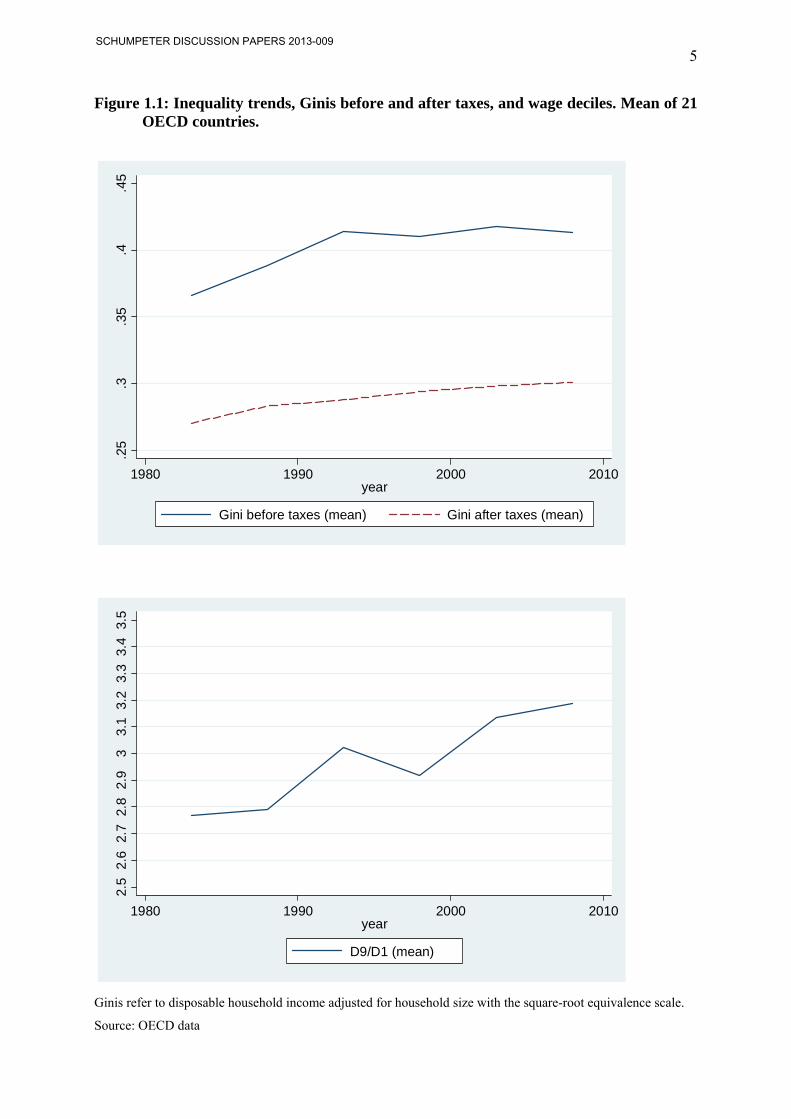
The (almost) universal rise in inequality (see Figure 1.1 and Section 4) is often interpreted as

the market response to changing economic conditions. Skill-biased technological progress and

globalization have shifted labor demand in favor of higher skills, requiring a wider wage

distribution – so the argument goes. Higher inequality reflects the new equilibrium, where

some gain because their marginal productivity rises and others lose because their contribution

to production falls. Marginal productivity determines wages, therefore higher inequality

reflects a new Pareto optimum, which cannot be changed without substantial losses in

efficiency, the so-called ‘big tradeoff’. Countries either adapt to the market requirements

allowing for more inequality or they will suffer from high and persistent unemployment, low

employment respectively (the two-sides of the coin view).

But higher inequality may actually reflect market failure rather than a Pareto optimal

distribution. Allowing for market imperfections in the analysis may produce very different

conclusions. With imperfect labor markets, firms may use wage-setting power. With

imperfect capital markets, inequality will reproduce inequality, creating a class structure,

which may become structural with increasing polarization of the income distribution.

However, even the fiercest advocates of inequality argue that society’s self-interest should not

allow extreme poverty among sections of the population, because crime, violence, and riots

may result. Aside from such extremes, inequality is beneficial (Welch 1999). But even less

extreme outcomes may be costly for society: overall beneficial policies may be blocked in

overly unequal societies either at the high end (e.g. securing privileges) or the low end in fear

of insecurity (e.g. resistance to technological change). Alan Krueger (2003) also mentions

access to political elites and stronger influence on the formulation of policy. Finally, people

care about their relative income positions: Keynes’s (1936) major explanation for resistance

to nominal wage reductions has been confirmed by recent research.

It has been argued that low income is transitory, i.e. that today’s low paid workers will move

up the income ladder, or that workers have other undeclared incomes, live in households with

several other incomes (e.g. Feldstein 1999). High and rising income inequality is even

presented as an opportunity: higher individual returns to education may positively influence

the individual’s decision to invest in human capital (Welch 1999). Almost everybody – at

least rhetorically – favors equality of opportunity, but opportunities to enroll in education are


4

in fact severely influenced by family backgrounds, institutional frameworks, access to

educational services and other socio-economic variables such as neighborhoods, role models,

attitudes etc. Inequality reproduces inequality and puts a long shadow on societies. The

public sector not only influences monetary incomes but also ‘extended incomes’, i.e. access to

publicly provided services, which are more important at the lower end of the distribution.

Taxes may discourage labor supply1 but taxes can enable (more) equal access to education,

more equality of opportunities, which seems to affect participation in labor markets

positively. Furthermore, in a dynamic economy, educational services may be especially

important, because to function in a complex society requires a minimum level of education.

Moreover, better education may enhance technological advancement and facilitate adaptation

to rapidly changing environments.2 Education may create positive spillovers, i.e. individuals’

investment in human capital may be sub-optimal, especially if households face credit

constraints – as they of course frequently do. Overcoming these impediments is not only

socially but also economically beneficial. Moreover, individual productivity derived from

education will depend on the overall educational level of society. Broad access to public

education would probably benefit society most if preschool education were enhanced.3

In this paper we investigate the hypothesis of the ‘big tradeoff’ with respect to the labor

market outcome. The next section, focusing on natural rate theory and rising inequality,

briefly discusses the theoretical background and empirical income distributions. The third

section investigates the relation between inequality and opportunity and the long-run effects

of inequality. In the fourth section we describe our cross-country longitudinal data set

followed by our empirical analysis of the relation between inequality, redistribution and labor

market outcomes in highly industrialized (OECD) countries. We use several indicators for

labor market performance (unemployment rates, employment to population rates, hours

worked per head of population) and inequality/redistribution respectively (decile ratios, Ginis,

a measure for the strength of redistribution). Section 6 concludes with our main finding.

1 The neoclassical labor supply model is theoretically indeterminate: the labor supply function may be forward- or backward-bending depending on the strength of the substitution and the income effect. The latter is in the theory always negative – higher unearned income reduces labor supply. Thus the model-immanent conclusion is that rising non-work incomes reduce labor supply. 2 A social security net may also improve the acceptance of technological change. 3 Heckman/Carneiro, (2003).


5

Figure 1.1: Inequality trends, Ginis before and after taxes, and wage deciles. Mean of 21 OECD countries.

.2

5.3

.35

.4.4

5

1980 1990 2000 2010year

Gini before taxes (mean) Gini after taxes (mean)

2.8

2.9

33.

13.

22.

52.

62.

73.

33.

43.

5

1980 1990 2000 2010year

D9/D1 (mean)

Ginis refer to disposable household income adjusted for household size with the square-root equivalence scale.

Source: OECD data


6

2. “Natural rate theory” and rising inequality

“Natural rate theory” – the hypothesis that national institutional frameworks generate a unique

equilibrium unemployment rate resulting from utility maximization of economic agents –

dominated economic policy for decades. Almost universally accepted, it interpreted

unemployment no longer as a waste of (human) resources but rather as the result of an

optimization process within a given institutional setting, i.e. as a structural problem. That

wages reflect marginal productivity is arguably one of the most accepted assumptions in

economics: high-wage earners simply contribute a lot whereas low wages imply small

contributions.4 Equating wages with individual marginal productivity – i.e. with the

individual’s contribution to the economy – often leads proponents of natural rate theory to

interpret the rising incomes of top earners to be Pareto-efficient. High paid individuals only

get what they deserve, what they contribute. Reducing their incomes – directly or through

taxes – will frustrate efforts, the pie will shrink and nobody will be better off. Let the market

determine wages and there will be “full employment” – meaning that actual unemployment is

at the “natural rate”.

High-wage workers’ incomes do not adversely affect the income of low-wage workers. High

wages are earned because they represent the individual’s contribution to production – that is

marginal product theory. And consequently – as claimed by Martin Feldstein (1999) and

others5 – an increase of income at the top of the pay-scale, even with constant wages at the

lower end, should be seen as Pareto–efficient. Why not improve the situation of some, if

others do not have to suffer? If wages reflect marginal productivity6, policy interventions that

compress the wage structure – especially at the low-end through legal minimum wages,

entitlements to transfers etc. – will cut off employment and cause unemployment.7 A

compressed wage structure deviating from the distribution of productivity is in this view

costly, as it will exclude workers with lower productivity from employment.8

4 Joseph Stiglitz (2013, INET video, How America As Land of Opportunity Has Vanished) said that he wishes the assumptions were true because that would prevent bankers receiving high bonuses. 5 Becker/Murphy (2007), Welch (1999). 6 Card (1996) found that the dispersion of pilots’ compensation increased substantially after the deregulation of the US airline industry. 7 The strong theoretical prior might explain the vociferous arguments by the heads of the leading economic research institutes against any potential legal minimum wage in Germany (Sinn et al. 2008). However, if the relation between pay and marginal productivity is not that strong, if firms have at least some discretion to determine wages (Manning 2003), the effects of minimum wage laws will not be as clear as in the textbook model. Card and Krueger’s (1995) finding that a rise in the legal minimum wage of almost 20% in New Jersey did not lead to employment losses has resulted in continuing intense discussion, even after 20 years. 8 Conversely, it is argued that integration of the unemployed requires a widening of wage distribution.


7

The “Big Tradeoff” (Okun 1975) between efficiency and equity was established on the

grounds that taxing high incomes creates a disincentive to work or effort at the upper end of

the pay-scale, while transfers have a similar effect at the lower end. If we assume a world

without market power, raising taxes may have adverse effects, but there may also be (at least)

two effects related to redistribution. Taxes may discourage the labor supply, but taxes can

enable (more) equal access to education and hence more equality of opportunity, which seems

to affect participation in labor markets positively. Labor market behavior deduced from these

assumptions produced a strong prior on any measure that might lead to wage compression,

especially at the lower end of the wage scale.9 The less skilled, so the argument went, were

excluded from jobs, being priced out of the market by enforced and excessively high

minimum wages – i.e. by compression of wage distribution from below. Countries must

therefore choose between higher inequality or higher unemployment.

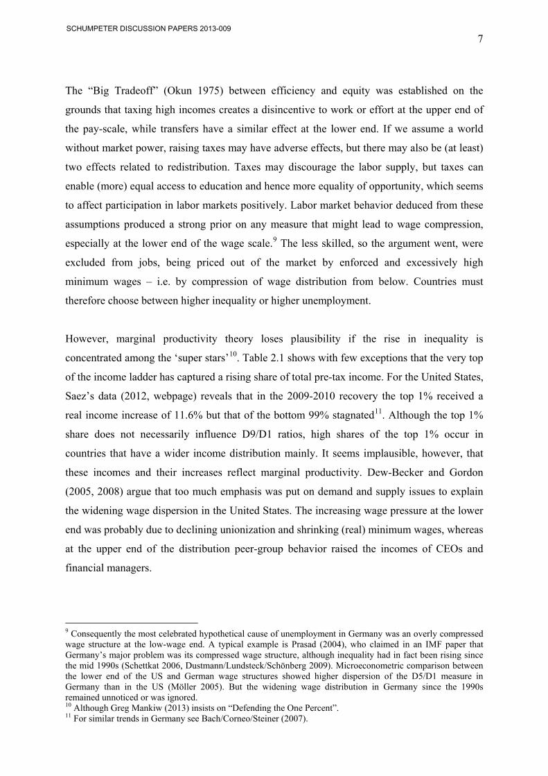
However, marginal productivity theory loses plausibility if the rise in inequality is

concentrated among the ‘super stars’10. Table 2.1 shows with few exceptions that the very top

of the income ladder has captured a rising share of total pre-tax income. For the United States,

Saez’s data (2012, webpage) reveals that in the 2009-2010 recovery the top 1% received a

real income increase of 11.6% but that of the bottom 99% stagnated11. Although the top 1%

share does not necessarily influence D9/D1 ratios, high shares of the top 1% occur in

countries that have a wider income distribution mainly. It seems implausible, however, that

these incomes and their increases reflect marginal productivity. Dew-Becker and Gordon

(2005, 2008) argue that too much emphasis was put on demand and supply issues to explain

the widening wage dispersion in the United States. The increasing wage pressure at the lower

end was probably due to declining unionization and shrinking (real) minimum wages, whereas

at the upper end of the distribution peer-group behavior raised the incomes of CEOs and

financial managers.

9 Consequently the most celebrated hypothetical cause of unemployment in Germany was an overly compressed wage structure at the low-wage end. A typical example is Prasad (2004), who claimed in an IMF paper that Germany’s major problem was its compressed wage structure, although inequality had in fact been rising since the mid 1990s (Schettkat 2006, Dustmann/Lundsteck/Schönberg 2009). Microeconometric comparison between the lower end of the US and German wage structures showed higher dispersion of the D5/D1 measure in Germany than in the US (Möller 2005). But the widening wage distribution in Germany since the 1990s remained unnoticed or was ignored. 10 Although Greg Mankiw (2013) insists on “Defending the One Percent”. 11 For similar trends in Germany see Bach/Corneo/Steiner (2007).


8

Nevertheless, economic policy was guided by theories claiming that reducing taxes for high-

income earners would generate social benefits, because the income elite would raise their

efforts, which would result in higher growth also benefiting the lower end of the wage

distribution.12 Put money to the top and it would eventually trickle down. Consequently, top

marginal income-tax rates fell by 20%-pts in the OECD average from 1980 to the mid 2000s

(OECD 2012). In other words, measures mainly based on theoretical deductions from an

idealized model became general guidelines for economic policy. “Natural rate theory” and

‘rational expectations’ were the yardsticks used to evaluate economic policy. Markets were

assumed always to perform optimally if not disturbed by public policy. The public sector

should therefore be restricted to a minimum. The OECD’s Jobs Study (1994) was designed

according to “natural rate theory”, which diffused even into the thinking of social democratic

politicians (New Labour, German Social Democrats). Deregulation of European welfare state

institutions was claimed to be the springboard for a ‘Great European Job Machine’ but, as

Richard Freeman (2005) showed, the magnitude of this IMF claim was totally implausible.

Nevertheless, it suggested to Spain, Portugal, and other countries suffering from the banking

crisis that recovery requires reforms (mainly labor market reforms), i.e. austerity programs,

lower wages and rising inequality.13

Table 2.1: Share of income and change in the share, top 1%, wage distribution

US

A

GB

R

CA

N

DE

U

CH

E

IRL

PR

T

ITA

JPN

NZ

L

AU

S

FR

A

ES

P

FIN

BE

L

DN

K

NO

R

SW

E

NL

D

share of income top 1%(%)

2007 18.3 14.3 13.3 11.1 10.5 10.3 9.8 9.5 9.2 9.0 8.9 8.9 8.8 8.6 7.7 7.4 7.1 6.9 5.7

1990 13.0 9.8 9.2 10.9 9.7 6.6 7.2 7.8 8.1 8.2 6.3 8.2 8.4 4.6 6.3 5.1 4.4 4.4 5.6

2007-1990 [%-pts.] 5.3 4.5 4.1 0.2 0.8 3.7 2.6 1.7 1.1 0.8 2.6 0.7 0.4 4 1.4 2.3 2.7 2.5 0.1

D9/D1

2007 4.8 3.6 3.7 3.2 3.8 4.3 2.3 3.1 2.9 3.3 2.9 3.5 2.5 2.3 2.7 2.2 2.3 2.9

1990 4.3 3.4 2.6 4.1 2.2 3.2 2.4 2.8 3.3 3.8 2.5 2.3 2.2 2.0 2.8

2007-1990 0.5 0.2 0.6 -0.3 0.1 -0.1 0.5 0.5 -0.4 -0.3 0.0 0.0 0.5 0.3 0.1

Source: Economic Policy Reforms 2012 - Going for Growth –OECD. Note: year 1990 for Germany, Ireland and Belgium. Correlations between the share of the top 1% incomes and the D9/D1 measure are .76 (2007) and .58 (1990).

12 Measures of inequality are usually based on monetary incomes before or after taxes. However, there is a substantial amount of indirect income, services in kind, that can have extremely different effects on inequality. 13 Austerity programs and cuts in public services affect lower income households more than higher income households (see OECD 2011).


9

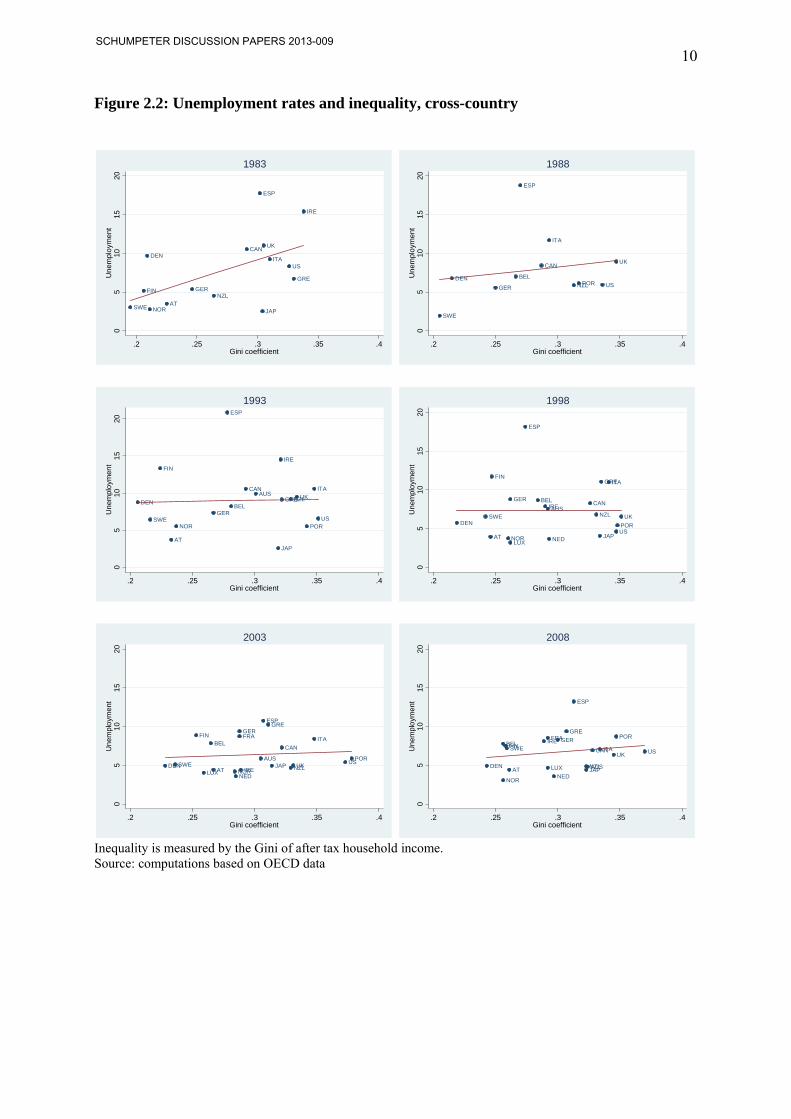
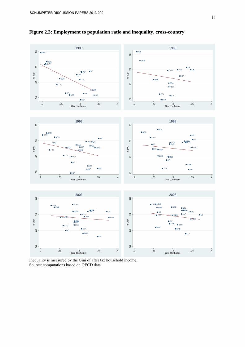
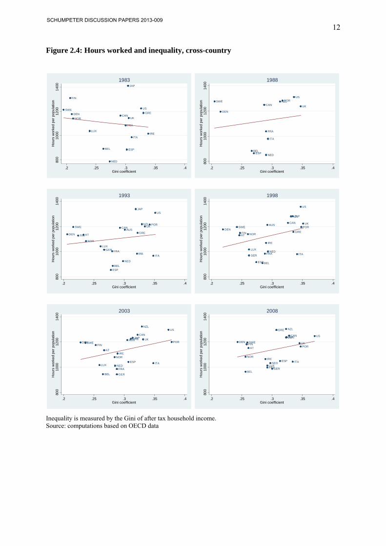
Figures 2.2 to 2.4 display the cross-country relations of labor market variables and inequality

based on 15 to 21 OECD countries (see section 4 for a detailed description). For

unemployment rates (Figure 2.2) the relationship is flat, i.e. it is not true that more unequal

economies show lower unemployment rates. Similarly for the employment-population ratio

(Figure 2.3), where the relation is, if anything, negative, i.e. higher inequality is related to a

lower employment-population ratio. Even if we use hours worked per head of population

(Figure 2.4) we do not find a strong relation. However, if one focuses on the US and

compares its performance to some European countries, one may get a stronger relation

between labor market performance and inequality. But this is a very selective approach,

although it has substantially influenced the debate on transatlantic differences in employment

trends. If this seems a surprising result from a first inspection of the data, it actually confirms

the results of many earlier studies.

Past empirical research often failed to identify the responsibility of institutional structures for

major differences in transatlantic employment trends (e.g. Glyn/Howell/Schmitt 2006,

Howell/Baker/Glyn/Schmitt 2007, Schettkat 2005, 2008)14. Astonishingly enough, it is only

since the end of 1980 that US unemployment rates have been lower than German rates (see

Buttler/Franz/Soskice/Schettkat 1995). Rather than casting doubt on the “natural rate theory”,

however, this led to the neglect of differences in macro-economic policies and corresponding

institutions15. Flow and duration analysis of unemployment and vacancies in the US and

Germany showed great mobility, suggesting that Germany was suffering from aggregate

demand deficiency rather than labor market rigidity (Schettkat, 1992). Institutional change in

Germany from the 1980s to the 2000s fails to explain the rise in unemployment. Reforming

institutions should have lowered rather than increased unemployment in Germany in that

period (Carlin/ Soskice, 2008).

14 Heckman, Ljunge and Ragan (2006) fiercely criticize the revised OECD view, arguing that the analysis of aggregate data is flawed, and that the unemployment rate is not the right measure, because corporatist countries hide unemployment in active labor market programs, early retirement, etc. 15 Solow (2008), Schettkat Sun (2009)


10

Figure 2.2: Unemployment rates and inequality, cross-country

AT

CANDEN

FIN GER

GRE

IRE

ITA

JAP

NZL

NOR

ESP

SWE

UK

US

05

1015

20U

nem

plo

ymen

t

.2 .25 .3 .35 .4Gini coefficient

1983

BEL

CAN

DEN

GER

ITA

NZLPOR

ESP

SWE

UK

US

05

1015

20U

nem

plo

ymen

t


1988

AUS

AT

BEL

CAN

DEN

FIN

GER

GRE

IRE

ITA

JAP

NZL

NOR POR

ESP

SWE

UK

US

05

1015

20U

nem

plo

ymen

t


1993

AUS

AT

BEL CAN

DEN

FIN

GER

GRE

IRE

ITA

JAPLUX

NED

NZL

NOR

POR

ESP

SWE UK

US

05

1015

20U

nem

plo

ymen

t


1998

AUS

AT

BELCAN

DEN

FIN FRAGER

GRE

IRE

ITA

JAPLUX

NED

NZLNOR

POR

ESP

SWE UKUS

05

1015

20U

nem

plo

ymen

t


2003

AUSAT

BELCAN

DEN

FINFRAGER

GRE

IREITA

JAPLUX

NED

NZL

NOR

POR

ESP

SWEUK US

05

1015

20U

nem

plo

ymen

t

.25 .3 .35 .4.2Gini coefficient

2008

Inequality is measured by the Gini of after tax household income. Source: computations based on OECD data


11

Figure 2.3: Employment to population ratio and inequality, cross-country

BEL

CAN

DENFIN

FRAGER

GRE

IREITA

JAP

LUX

NED

NOR

ESP

SWE

UKUS

5060

7080

E-p

op


1983

BEL

CAN

DEN

FRA

GER

ITA

NED

NZL

POR

ESP

SWE

UKUS

5060

7080

E-p

op


1988

AUS

AT

BEL

CAN

DEN

FIN

FRA

GER

GRE

IRE ITA

JAP

LUX

NED

NZL

NOR

POR

ESP

SWE

UK

US

5060

7080

E-p

op


1993

AUSAT

BEL

CAN

DEN

FIN

FRA

GER

GRE

IRE

ITA

JAP

LUX

NEDNZL

NOR

POR

ESP

SWEUK

US

5060

7080

E-p

op


1998

AUS

AT

BEL

CAN

DEN

FIN

FRA

GER

GRE

IRE

ITA

JAP

LUX

NEDNZL

NOR

POR

ESP

SWE

UKUS

5060

7080

E-p

op


2003

AUSAT

BEL

CAN

DEN

FIN

FRA

GER

GRE

IRE

ITA

JAP

LUX

NED NZL

NOR

POR

ESP

SWE

UK

US

5060

7080

E-p

op


2008



12

Figure 2.4: Hours worked and inequality, cross-country

BEL

CANDEN

FIN

FRA

GRE

IREITA

JAP

LUX

NED

NOR

ESP

SWE

UK

US

800

1000

1200

1400

Ho

urs

wor

ked

per

pop

ula

tion


1983

BEL

CAN

DEN

FRA

ITA

NED

NZLPOR

ESP

SWE

UK

US

800

1000

1200

1400

Ho

urs

wor

ked

per

pop

ula

tion


1988

AUS

AT

BEL

CAN

DEN FIN

FRAGER

GRE

IREITA

JAP

LUX

NED

NZL

NOR

POR

ESP

SWE UK

US

800

1000

1200

1400

Ho

urs

wor

ked

per

pop

ula

tion


1993

AUS

AT

BEL

CAN

DENFIN

FRAGER

GRE

IRE

ITA

JAP

LUXNED

NZL

NOR

POR

ESP

SWEUK

US80

010

0012

0014

00H

our

s w

orke

d p

er p

opu

latio

n


1998

AUS

AT

BEL

CAN

DENFIN

FRA

GER

GRE

IRE

ITA

JAP

LUX NED

NZL

NOR

POR

ESP

SWEUK

US

800

1000

1200

1400

Ho

urs

wor

ked

per

pop

ula

tion


2003

AUS

AT

BEL

CAN

DENFIN

FRAGER

GRE

IREITA

JAP

LUXNED

NZL

NOR

POR

ESP

SWE UK

US

800

1000

1200

1400

Ho

urs

wor

ked

per

pop

ula

tion


2008



13

As the OECD (2004) states, micro-econometric studies focusing on wage compression in

Europe (the main factor used to explain high European unemployment) failed to establish

evidence that wage compression had caused labor market problems (the OECD cites

Nickell/Bell 1996, Card/Kramarz/Lemieux 1996, Krueger/Pischke 1997, Freeman/Schettkat

2000). But the same OECD study concluded that, ‘nevertheless’ rising wage inequality in the

US was the market response to demand shifting away from less skilled labor, and that this

would also be the right cure for Europe. In Europe, minimum wages (statutory, negotiated or

implied by social assistance and unemployment benefits) and generous unemployment

benefits had prevented wage inequality from rising, but the result was high and rising

unemployment.


14

3. Perfect-market assumptions and skill formation

Increasing inequality in the US, Welch (1999) emphatically claimed in his Ely lecture “In

Defense of Inequality”16, opened investment opportunities for new entrants into the labor

force because of higher returns to education17. Welch interprets the simultaneous occurrence

of rising wage dispersion and increasing enrollment in higher education as evidence in favor

of his hypothesis. What happened, then, in the Scandinavian countries where educational

attainment increased substantially but wage differentials were small? High wage dispersion

between education or skill groups may enhance human capital investment, but within

educational groups high wage dispersion raises ex ante the risk to that investment, i.e. it may

be a disincentive (Agell, 1999).18 Richard Freeman – in a paper with Dan Devroye (Devroye/

Freeman 2001) – used skills as measured in the International Adult Literacy Survey (OECD

1997) (i.e. an output variable) rather than education (an input variable) to investigate US skill

and wage distribution. They found higher wage dispersion within narrowly defined skill

groups (10 percentage points skill groups on a scale from 0 to 500 points) in the US than in

the entire Swedish economy. 19

If ability is equally distributed, equality of opportunity implies a low elasticity20 in the socio-

economic status of consecutive generations. Naturally, in all countries the influence of parents

on their children’s educational and income achievements is strong,21 but the strength of the

relation varies and seems to be substantially affected by public policy. In a strictly privately

financed educational system, the link between the parents’ income position and educational

attainment of their children will be strong. Unequal income distribution in the parents’

16 Becker and Murphy 2007, Feldstein (1999), for example, argue along similar lines. 17 Returns to education are usually based on years of education rather than on the actual costs. 18 Even if the supply of highly skilled labor increases, the ‘college wage premium’ may also increase if demand increases even faster (see Katz/Murphy 1992). Card/ DiNardo (2002) investigated the plausibility of skill-biased technological change and concluded that institutional changes like the declining influence of unions and the decline in the legal minimum wage were a more plausible cause of rising wage inequality in the US. 19 Devroye/Freeman observe that wages in the US may be ex ante equal for ‘identical’ persons, but contracts make future earnings depend on the success of the company, which is outside the control of the individual – i.e. Americans conclude risky contracts. The authors argue that this is different from wagering on luck. Thurow (1975) argues that on-the-job training is causing heterogeneity in wages. 20 Intergenerational income elasticity is often measured by the (log) relative income position of the children to the relative income position of the parents. That is, if the children’s income relative to the mean income is high and parents had a similar income position, the elasticity is high, if the parents had a low income position, the elasticity is low.

ln(Yci/Yc.) = a + b ln(Ypi/Yp.) + u where Yci/Yc. = relative income of children, Ypi/Tp. = relative income of parents, coefficient b = elasticity. 21 Neighborhood effects will not only arise because of differences in access to resources, but also social interaction and role models may be missing in less wealthy neighborhoods with low educational resources (Durlauf 1992).


15

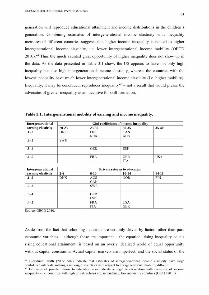
generation will reproduce educational attainment and income distributions in the children’s

generation. Combining estimates of intergenerational income elasticity with inequality

measures of different countries suggests that higher income inequality is related to higher

intergenerational income elasticity, i.e. lower intergenerational income mobility (OECD

2010).22 Thus the much vaunted great opportunity of higher inequality does not show up in

the data. As the data presented in Table 3.1 show, the US appears to have not only high

inequality but also high intergenerational income elasticity, whereas the countries with the

lowest inequality have much lower intergenerational income elasticity (i.e. higher mobility).

Inequality, it may be concluded, reproduces inequality23 – not a result that would please the

advocates of greater inequality as an incentive for skill formation.

Table 3.1: Intergenerational mobility of earning and income inequality.

Gini coefficients of income inequality Intergenerational earning elasticity 20-25 25-30 30-35 35-40 .1-.2 DNK FIN

NOR CAN AUS

.2-.3 SWE

.3-.4 GER

ESP

.4-.5 FRA GBR ITA

USA

Private returns to education Intergenerational

earning elasticity 2-6 6-10 10-14 14-18 .1-.2 DNK AUS

CAN NOR FIN

.2-.3

SWE

.3-.4

GER ESP

.4-.5

FRA ITA

USA GBR

Source: OECD 2010.

Aside from the fact that schooling decisions are certainly driven by factors other than pure

economic variables – although these are important – the equation ‘rising inequality equals

rising educational attainment’ is based on an overly idealized world of equal opportunity

without capital constraints. Actual capital markets are imperfect, and the social status of the 22 Björklund/ Jäntti (2009: 502) indicate that estimates of intergenerational income elasticity have large confidence intervals, making a ranking of countries with respect to intergenerational mobility difficult. 23 Estimates of private returns to education also indicate a negative correlation with measures of income inequality – i.e. countries with high private returns are, in tendency, low inequality countries (OECD 2010).


16

family (parents) strongly influences the academic achievements of students, as the shocking

results of work by Fox, Connolly, and Snyder (2005) revealed. Sorting students by their math

performance in the 8th grade into 3 groups (low, medium, high), completed bachelor’s

degrees rise with family income within all 3 groups. But, most shockingly, the proportion of

students from low-income families who scored high in math in the 8th grade – ‘the very able

poor’ – is the same as that of low-scoring students from high-income families – ‘the less able

rich’. Money beats ability.

Public expenditure on education increases extended income – i.e. pecuniary income extended

by in-kind transfers24 – substantially, especially in the lower segment of income distribution.

For the OECD 21 (not including the ‘new’ OECD countries) the percentage expenditure on

in-kind services (compared to cash transfers) in GDP is 13.4%, accounting for 13.2% of GDP.

In general, public expenditure has a strong impact on inequality indicators, reducing Gini

coefficients by around 20% (OECD 2011: 317 Table 8.2). Educational services account for

5.1% of this. Thus the relation between changes in public service provision and reductions in

inequality appears quite strong. Countries that reduced public service provision experienced

an increase in inequality and vice versa (see OECD 2011: Fig 8.11). Restricting public

services to the minimum will, therefore, harm efforts to equalize opportunities and may

reduce growth potential (Dauderstädt 2012).

Although data is scarce, analysis of the OECD’s 2010 report reveals that public policy can

substantially promote equality of educational attainment. Plotting their fathers’ skill levels on

the horizontal against children’s skill levels on the vertical reveals a relatively steep function,

i.e. a high correlation between the skills of the two generations. The functions do not change

much between different cohorts. However, for Norway – the only country cited in the OECD

analysis – the function is much flatter for the younger cohort than for the older one. And, most

importantly, the function has flattened because children from parents with lower educational

attainment have achieved higher scores.

24 Following work of the ‘Luxembourg income study group’ and others, the OECD provided new estimates of extended incomes including in-kind benefits from public services.


17

4. Data and method

Naturally, country studies rely on few observations, and aggregate analysis using countries as

units may hide other substantial differences. Nevertheless, countries may serve very well for

an investigation of fundamental relations. If inequality has such dominant effects, one would

expect it to influence measures of employment both across and within countries. To analyze

the impact of inequality on labor markets we constructed a panel data set derived from OECD

data. Cross-country analysis may be insufficient because employment variables are influenced

by more factors than distribution. Thus wage and income distribution may be narrower in one

country because the dispersion of skills is lower there. For example, Sweden is known for its

comparatively narrow wage distribution, but Sweden also has a very narrow skill distribution

(Devroye/Freeman 2001). So, leaving aside the issue of redistribution, the result can hardly be

unexpected. The longitudinal aspect in our data should identify such issues. If Swedish skill

distribution remains roughly constant, the impact of narrow skill distribution should be

captured in a country effect. To eliminate the effect of unobserved variables, the following

analysis uses first differences. If a causal relation between inequality/redistribution and

employment variables exists, changes in the independent variable – redistribution/inequality –

should influence the development of the dependent variables.

Because not all data were available for every country and every year, we used an unbalanced

panel of 21 highly industrialized OECD25 countries during the period 1980-2010. To avoid

autocorrelation we took means over 5-year periods, which resulted in six different time

periods (1981-1985, 1986-1990, 1991-1995, 1996-2000, 2001-2005 and 2006-2010). Labor

market indicators – the dependent variables – used are employment-population rates, hours

worked per head of population (18-65) and unemployment rates. The independent variables –

inequality and redistribution – are Ginis26 before and after taxes, decile ratios (D9-D1, D9-

D5, D5-D1), and a measure of redistribution (red_m). Ginis are computed on the basis of

household income adjusted with equivalence scales, and are thus influenced among other

things by the participation of household members in labor markets. For example, if a higher

share of women is working, it may reduce the Gini based on household income, which may

25 OECD countries included are Australia, Austria, Belgium, Canada, Denmark, Finland, France, Greece, Germany, Italy, Ireland, Japan, Luxembourg, Netherlands, New Zealand, Norway, Portugal, Spain, Sweden, the United Kingdom and the United States. 26 Gini coefficients usually refer to family or household income (before or after taxation), i.e. Ginis (usually) do not reflect the distribution of wages. Decile ratios of (gross) wages are therefore a more direct indicator for inequality in the labor market.


18

not reflect an equal distribution of wages but rather a compensating labor supply effect.

Therefore, a more direct measure for inequality potentially affecting labor market outcomes is

decile-ratios of wages.

The redistribution measure was computed as the ratio of the Gini coefficient before taxes

divided by the Gini coefficient after taxes [rdm=(Gini before taxation)/(Gini after taxation)].

Values above 1 indicate less inequality after taxation, values below 1 indicate more inequality

after taxation. The latter is empirically not observed, i.e. all countries equalize income

distribution through taxes. According to conventional reasoning a high degree of

redistribution should discourage high wage labor supply (because some income is taxed

away) but also low wage labor supply (because transfers are available with little or no work).

Thus the redistribution measure may best capture the ‘big tradeoff’.

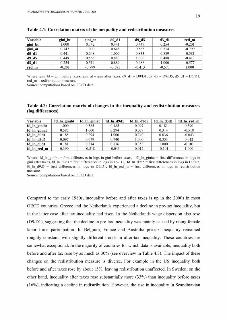
Table 4.1 displays the correlation matrix of the independent variables. The Ginis before

(gini_bt) and after (gini_at) taxes correlate highly but much more weakly with the decile

ratios of wages. Ginis (before and after taxes) seem to capture inequality in society in general

but are probably less suited to capture inequality in labor markets because of the household

context influencing the Ginis used. The decile wage ratios of the lower (d5_d1) and upper

(d9_d5) end of the wage scale both correlate highly with the overall decile ratio (d9-d1). The

redistribution measure (red_m) correlates negatively with all distribution measures, i.e. a

higher degree of redistribution goes together with less inequality. Apparently redistribution

affects the after tax Gini (gini_at) more strongly than the before tax Gini (gini_bt), indicating

what may be interpreted as successful redistribution. If redistribution were used to correct the

most unequal labor market outcomes, a positive correlation between the redistribution

measure and inequality variables should occur. Instead we find generally negative correlation

coefficients of the redistribution measure with all inequality variables, indicating that

economies that are already more equal also emphasize redistribution.


19

Table 4.1: Correlation matrix of the inequality and redistribution measures Variable gini_bt gini_at d9_d1 d9_d5 d5_d1 red_m gini_bt 1.000 0.742 0.441 0.449 0.254 -0.201 gini_at 0.742 1.000 0.648 0.565 0.514 -0.799 d9_d1 0.441 0.648 1.000 0.833 0.889 -0.581 d9_d5 0.449 0.565 0.883 1.000 0.488 -0.413 d5_d1 0.254 0.514 0.889 0.488 1.000 -0.577 red_m -0.201 -0.799 -0.581 -0.413 -0.577 1.000 Where: gini_bt = gini before taxes, gini_at = gini after taxes, d9_d1 = D9/D1, d9_d5 = D9/D5, d5_d1 = D5/D1, red_m = redistribution measure. Source: computations based on OECD data.

Table 4.2: Correlation matrix of changes in the inequality and redistribution measures (log differences) Variable fd_ln_ginibt fd_ln_giniat fd_ln_d9d1 fd_ln_d9d5 fd_ln_d5d1 fd_ln_red_m fd_ln_ginibt 1.000 0.585 0.185 0.097 0.181 0.390 fd_ln_giniat 0.585 1.000 0.294 0.079 0.314 -0.518 fd_ln_d9d1 0.185 0.294 1.000 0.740 0.836 -0.043 fd_ln_d9d5 0.097 0.079 0.740 1.000 0.353 0.012 fd_ln_d5d1 0.181 0.314 0.836 0.353 1.000 -0.101 fd_ln_red_m 0.390 -0.518 -0.043 0.012 -0.101 1.000 Where: fd_ln_ginibt = first differences in logs in gini before taxes, fd_ln_giniat = first differences in logs in gini after taxes, fd_ln_d9d1 = first differences in logs in D9/D1, fd_ln_d9d5 = first differences in logs in D9/D5, fd_ln_d9d5 = first differences in logs in D5/D1, fd_ln_red_m = first differences in logs in redistribution measure. Source: computations based on OECD data.

Compared to the early 1980s, inequality before and after taxes is up in the 2000s in most

OECD countries. Greece and the Netherlands experienced a decline in pre-tax inequality, but

in the latter case after tax inequality had risen. In the Netherlands wage dispersion also rose

(D9/D1), suggesting that the decline in pre-tax inequality was mainly caused by rising female

labor force participation. In Belgium, France and Australia pre-tax inequality remained

roughly constant, with slightly different trends in after-tax inequality. These countries are

somewhat exceptional. In the majority of countries for which data is available, inequality both

before and after tax rose by as much as 30% (see overview in Table 4.3). The impact of these

changes on the redistribution measure is diverse. For example in the US inequality both

before and after taxes rose by about 15%, leaving redistribution unaffected. In Sweden, on the

other hand, inequality after taxes rose substantially more (33%) than inequality before taxes

(16%), indicating a decline in redistribution. However, the rise in inequality in Scandinavian


20

countries occurred from a low level. In the overview table (Table 4.3) the numbers in

parentheses indicate the change in the redistribution measure from the 1980s to the 2000s.

Table 4.3: Countries by changes in Ginis before and after taxes [%] Gini before taxes Gini after taxes <= -5% -5%>= <=5% >5% <= -5%

GREECE (+)

NETHERLANDS (-)

-5%>= <=5%

BELGIUM (+)

FRANCE (-)

AUSTRALIA (-)

>5%

UNITED KINGDOM (-) NEW ZEALAND (-) CANADA (0) UNITED STATES (0) JAPAN (+) DENMARK (0) PORTUGAL (+) SWEDEN (-) GERMANY (-) FINLAND (-) ITALY (+) LUXEMBOURG (+) NORWAY (+)

Note: Change between the mean of 2006-2010 relative to the mean of 1981-1984; for some countries the reference is a later year; numbers in parentheses indicate the direction of change in the redistribution measure. Source: computations based on OECD data.


21

5. Inequality, redistribution and employment

To analyze the effects of inequality and redistribution on labor market outcomes, we

regressed first differences of the logs of the dependent variables (labor market indicators) on

first differences of the logs of the independent variables (distribution measures, redistribution

measure) with and without a set of controls (time (period) and country dummies):

Δlog(labor market indicatorit) = α0 + α1i,t Δlog(inequal-redisi,t) + α2t dt + α3i dci + uit

Where: labor market indicator= employment population rates, unemployment, hours worked per head of population, inequal-redistr = inequality, redistribution measure, dt = dummies for the periods, dc = dummies for countries, i = country index, t = time index, Δ=first difference (here between averages of 5 year periods)27

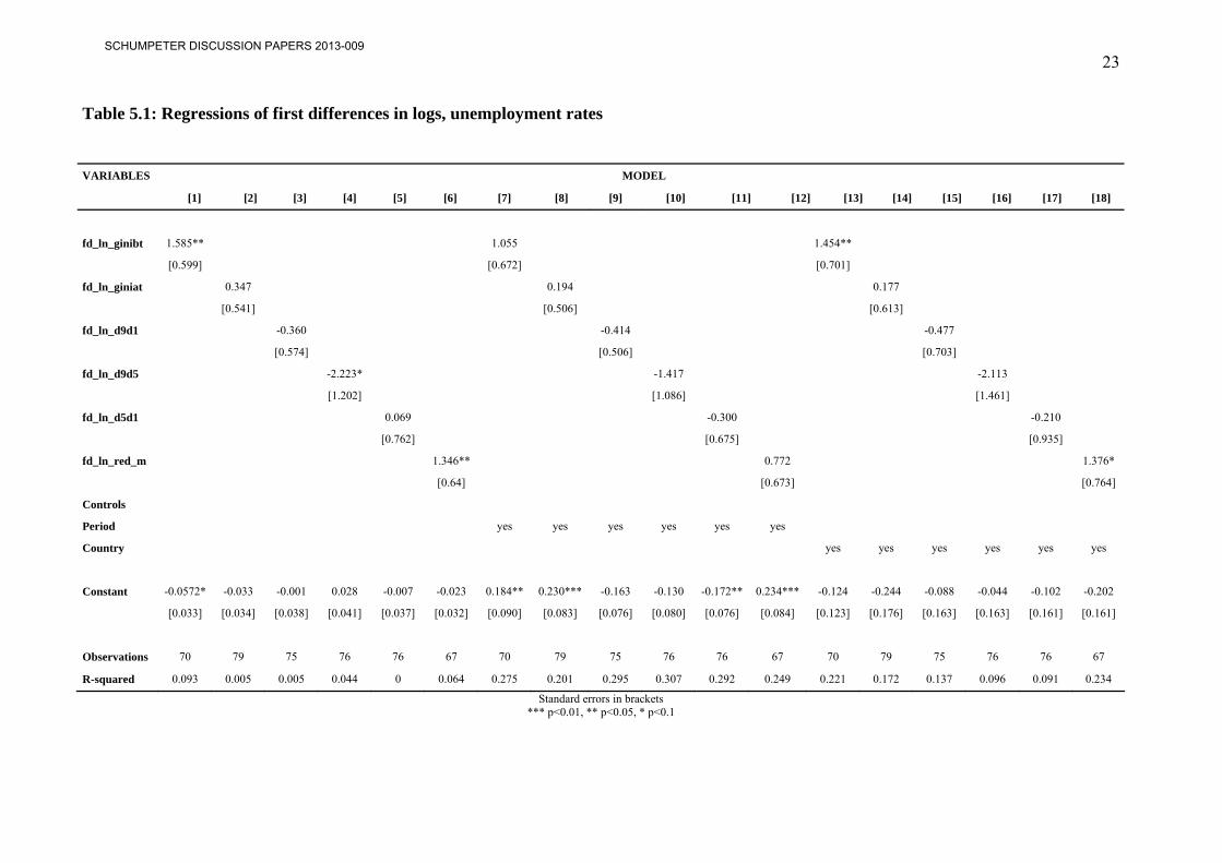
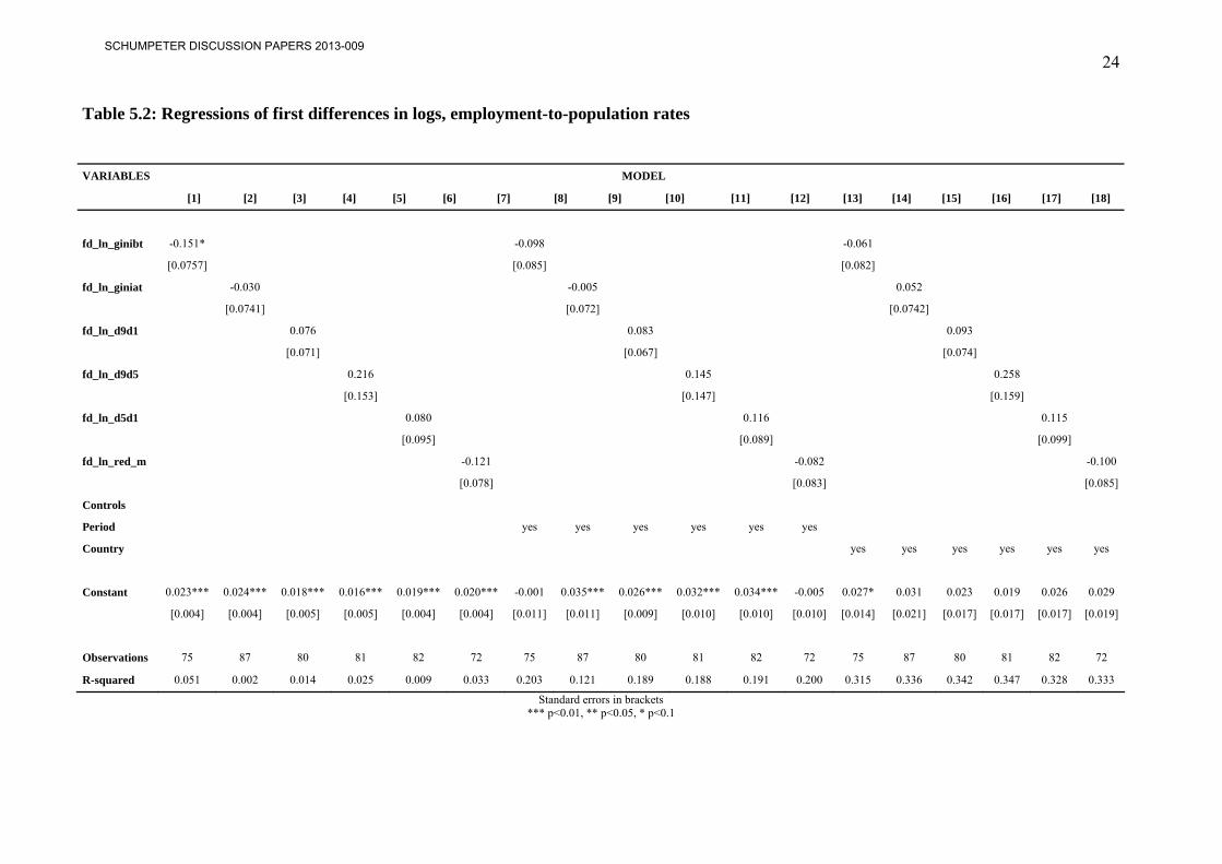
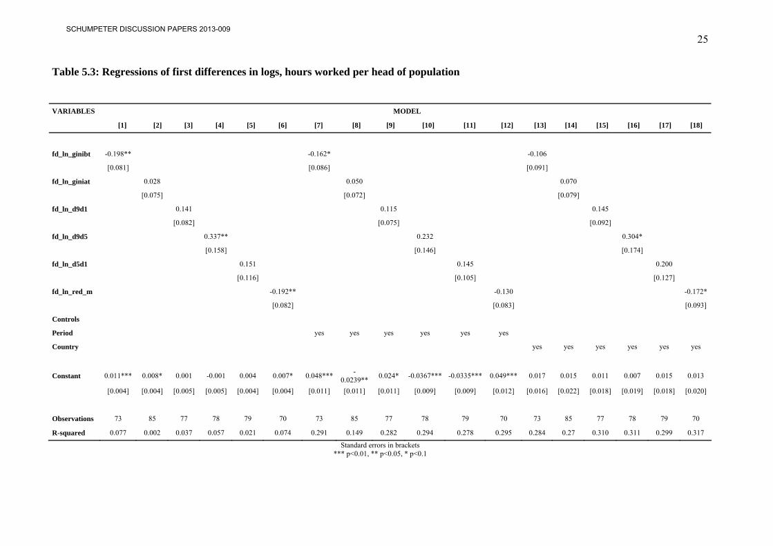
Tables 5.1 to 5.3 display the results of regressions of first differences of the logs of

unemployment rates, employment to population rates, and hours worked per head of

population in working age on inequality measures for the entire dataset, both without and with

controls (country and period effects) for the complete dataset.

The coefficients of changes (first differences) in inequality (Ginis) before taxes (fd_ln_ginibt)

show a positive effect on unemployment rates in models without controls (column 1, Table

5.1). With controls for period effects (column 7 in Table 5.1) the positive sign of the Gini

before taxes is insignificant, but it remains significantly positive in the model controlling for

country effects (columns 13 in Table 5.1). The latter emphasizes the relation over time and

may therefore better indicate actual causation. A positive sign is the reverse of the ‘two sides

of the coin’ metaphor, according to which one should either observe rising inequality or rising

unemployment. However, as mentioned above, the Ginis refer to (weighted) household

income, i.e. reverse causation may be important here. If unemployed workers find jobs, this

will lift the income of their households and may reduce inequality, which would be consistent

with the positive coefficient.

If rising inequality before taxes actually caused higher unemployment rates, one would also

expect a negative effect of the Gini before taxes (fd_ln_ginibt) on employment-to-population

rates. This effect, however, can only be observed with weak significance (10% significance

level) in model 1 (first column in Table 5.2) but not in the models with controls (columns 7

27 Following Blanchard/Wolfers (1999) we use averages over 5 year periods, which should reduce autocorrelation.


22

and 13). Similarly for hours worked per head of population. Without controls the Gini before

taxes lowers hours worked (column 1, Table 5.3) but with country-fixed effects (column 13)

the coefficient is lower and insignificant (columns 7 and 13).

Other inequality indicators which seem to influence changes in unemployment rates are

changes in the D9/D5 ratio (fd_ln_d9d5); but with controls the effect disappears. Only the

redistribution measure shows a positive sign with country-fixed effects, although the

significance is at a low level (10%, column 18 Table 5.1). These two measures (fd_ln_d95

and fd_ln_red_m) also affect hours worked per head of population in the expected direction

(positive for the D9D5 ratio, negative for the redistribution measure); but with controls the

significance is low in columns 16 &18 of Table 5.3 and even lower in columns 10 & 11. The

effects, however, cannot be discovered in the regression with the employment-to-population

rates as dependent variable (Table 5.2)

The only distribution variable whose changes seem to affect the labor market indicators is the

D9/D5 ratio. The positive effect on hours worked per head of population (Table 5.3, column

16) and the insignificant effect on the employment-to-population rate (Table 5.2, column 16)

is plausible if high wages and long hours correlate positively. But then the negative (although

insignificant effect) on unemployment rates is surprising. However, the hypothesis that rising

D5/D1 ratios affect participation and hours worked positively and unemployment rates

negatively is not confirmed by our data. For the redistribution measure (fd_ln_red_m) a

positive effect occurs in Table 5.1, i.e. rising redistribution occurs with rising unemployment

rates. Because the redistribution measure is constructed as the ratio of the Gini before taxes

divided by the Gini after taxes, the same endogeneity problem as for the Gini before taxes

(see above) may affect the result. But again the coefficient is only significant at the 10% level

(column 18 Table 5.1). Redistribution also seems to negatively affect hours worked (Table

5.3), which may be taken as confirmation of traditional hypotheses.


23

Table 5.1: Regressions of first differences in logs, unemployment rates VARIABLES MODEL

[1] [2] [3] [4] [5] [6] [7] [8] [9] [10] [11] [12] [13] [14] [15] [16] [17] [18]

fd_ln_ginibt 1.585** 1.055 1.454**

[0.599] [0.672] [0.701]

fd_ln_giniat 0.347 0.194 0.177

[0.541] [0.506] [0.613]

fd_ln_d9d1 -0.360 -0.414 -0.477

[0.574] [0.506] [0.703]

fd_ln_d9d5 -2.223* -1.417 -2.113

[1.202] [1.086] [1.461]

fd_ln_d5d1 0.069 -0.300 -0.210

[0.762] [0.675] [0.935]

fd_ln_red_m 1.346** 0.772 1.376*

[0.64] [0.673] [0.764]

Controls

Period yes yes yes yes yes yes

Country yes yes yes yes yes yes

Constant -0.0572* -0.033 -0.001 0.028 -0.007 -0.023 0.184** 0.230*** -0.163 -0.130 -0.172** 0.234*** -0.124 -0.244 -0.088 -0.044 -0.102 -0.202

[0.033] [0.034] [0.038] [0.041] [0.037] [0.032] [0.090] [0.083] [0.076] [0.080] [0.076] [0.084] [0.123] [0.176] [0.163] [0.163] [0.161] [0.161]

Observations 70 79 75 76 76 67 70 79 75 76 76 67 70 79 75 76 76 67

R-squared 0.093 0.005 0.005 0.044 0 0.064 0.275 0.201 0.295 0.307 0.292 0.249 0.221 0.172 0.137 0.096 0.091 0.234

Standard errors in brackets *** p<0.01, ** p<0.05, * p<0.1


24

Table 5.2: Regressions of first differences in logs, employment-to-population rates VARIABLES MODEL

[1] [2] [3] [4] [5] [6] [7] [8] [9] [10] [11] [12] [13] [14] [15] [16] [17] [18]

fd_ln_ginibt -0.151* -0.098 -0.061

[0.0757] [0.085] [0.082]

fd_ln_giniat -0.030 -0.005 0.052

[0.0741] [0.072] [0.0742]

fd_ln_d9d1 0.076 0.083 0.093

[0.071] [0.067] [0.074]

fd_ln_d9d5 0.216 0.145 0.258

[0.153] [0.147] [0.159]

fd_ln_d5d1 0.080 0.116 0.115

[0.095] [0.089] [0.099]

fd_ln_red_m -0.121 -0.082 -0.100

[0.078] [0.083] [0.085]

Controls



Constant 0.023*** 0.024*** 0.018*** 0.016*** 0.019*** 0.020*** -0.001 0.035*** 0.026*** 0.032*** 0.034*** -0.005 0.027* 0.031 0.023 0.019 0.026 0.029

[0.004] [0.004] [0.005] [0.005] [0.004] [0.004] [0.011] [0.011] [0.009] [0.010] [0.010] [0.010] [0.014] [0.021] [0.017] [0.017] [0.017] [0.019]

Observations 75 87 80 81 82 72 75 87 80 81 82 72 75 87 80 81 82 72

R-squared 0.051 0.002 0.014 0.025 0.009 0.033 0.203 0.121 0.189 0.188 0.191 0.200 0.315 0.336 0.342 0.347 0.328 0.333



25

Table 5.3: Regressions of first differences in logs, hours worked per head of population VARIABLES MODEL

[1] [2] [3] [4] [5] [6] [7] [8] [9] [10] [11] [12] [13] [14] [15] [16] [17] [18]

fd_ln_ginibt -0.198** -0.162* -0.106

[0.081] [0.086] [0.091]

fd_ln_giniat 0.028 0.050 0.070

[0.075] [0.072] [0.079]

fd_ln_d9d1 0.141 0.115 0.145

[0.082] [0.075] [0.092]

fd_ln_d9d5 0.337** 0.232 0.304*

[0.158] [0.146] [0.174]

fd_ln_d5d1 0.151 0.145 0.200

[0.116] [0.105] [0.127]

fd_ln_red_m -0.192** -0.130 -0.172*

[0.082] [0.083] [0.093]

Controls



Constant 0.011*** 0.008* 0.001 -0.001 0.004 0.007* 0.048***-

0.0239** 0.024* -0.0367*** -0.0335*** 0.049*** 0.017 0.015 0.011 0.007 0.015 0.013

[0.004] [0.004] [0.005] [0.005] [0.004] [0.004] [0.011] [0.011] [0.011] [0.009] [0.009] [0.012] [0.016] [0.022] [0.018] [0.019] [0.018] [0.020]

Observations 73 85 77 78 79 70 73 85 77 78 79 70 73 85 77 78 79 70

R-squared 0.077 0.002 0.037 0.057 0.021 0.074 0.291 0.149 0.282 0.294 0.278 0.295 0.284 0.27 0.310 0.311 0.299 0.317



26

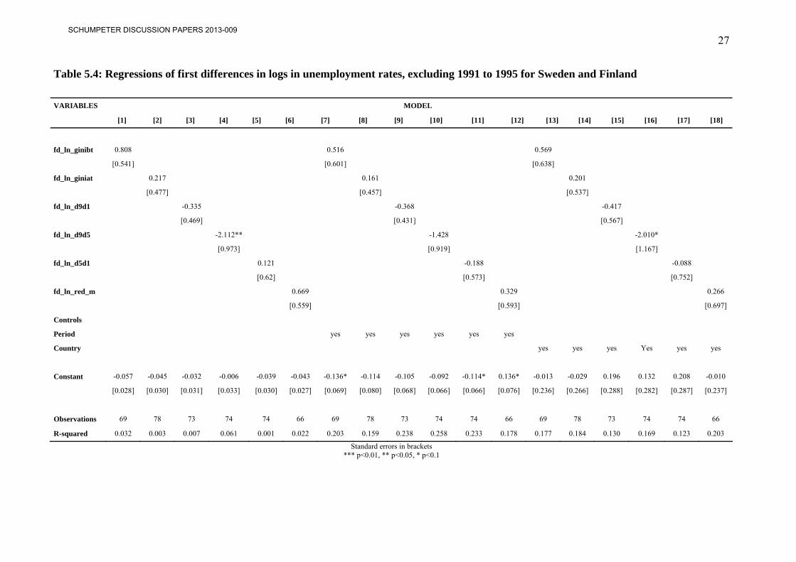
What, then, might explain the differences between the regression of unemployment rates on

inequality on the one hand and those of employment-to-population rates and hours worked on

the other? Why do we observe a positive coefficient for inequality on unemployment? Does

this represent actual causation? Unemployment rates show much higher volatility than either

employment-to-population rates or hours worked per head of population. The standard

deviation of the relative changes in unemployment rates (the first difference of the logs) in

our sample is 0.30, whereas it is 0.04 for employment-to-population rates and for hours

worked per head of population. Similarly for the maximum changes, which are 8

(employment-to-population rates) to 9 (hours worked) times higher for unemployment rates.

Changes in unemployment rates of 50% or more are not common, but they do happen. Such

unemployment shocks are hardly caused by institutional features, which can change labor

markets over a certain period but not in shock waves. In Sweden and Finland unemployment

rates more than doubled between the means of five year periods from 1986-1990 to 1991-

1995. This related to the financial crisis in Sweden and to the breakdown of demand from the

Soviet Union in Finland. Both Finland and Sweden have comparatively low but rising (see

Table 4.3) inequality indices, and these two countries experienced unemployment shocks. It is

this that mainly caused the positive coefficient of inequality on unemployment rates in the

regression displayed in Table 5.1. Excluding these two extreme cases28 leads to the results

presented in Tables 5.4 to 5.6.

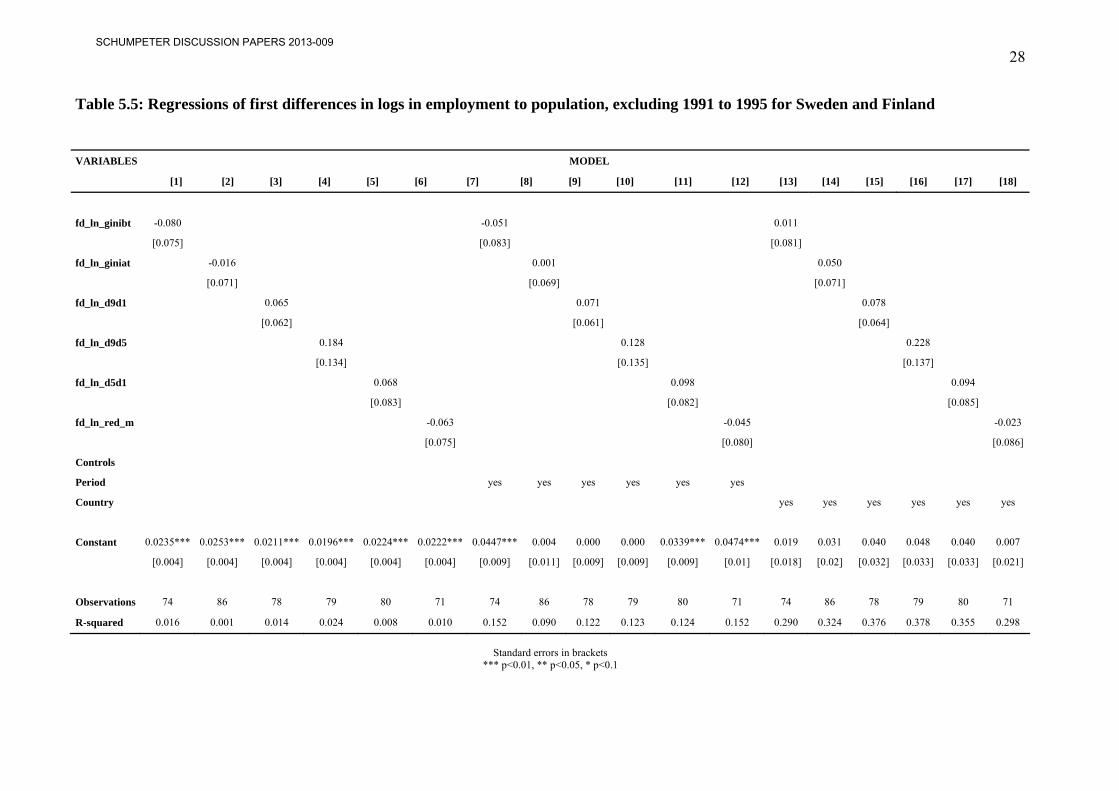
Without Sweden and Finland 1993 (actually the period 1991-1995), neither the first

differences of Ginis before or after taxes would contribute significantly to the variation in

unemployment rate changes. None of the distribution variables significantly affects the

employment-to-population ratios (Table 5.5); but, again, the D9D5 ratio seems to affect hours

worked, albeit only with low significance (Table 5.6 column 16).

Similar reasoning as for the unemployment shocks in Sweden and Finland may be adduced

for the 2006 to 2010 period when the ‘great recession’ hit the world’s economies.

Distributions probably changed slowly, but unemployment rose substantially. Controlling for

countries, and performing a sensitivity analysis with data limited to the period before 2005,

leaves the Gini before taxes significant; but again it is positive and driven by the rise in

unemployment in the early 1990s.

28 For Finland not all data was available for all periods.


27

Table 5.4: Regressions of first differences in logs in unemployment rates, excluding 1991 to 1995 for Sweden and Finland

VARIABLES MODEL

[1] [2] [3] [4] [5] [6] [7] [8] [9] [10] [11] [12] [13] [14] [15] [16] [17] [18]

fd_ln_ginibt 0.808 0.516 0.569

[0.541] [0.601] [0.638]

fd_ln_giniat 0.217 0.161 0.201

[0.477] [0.457] [0.537]

fd_ln_d9d1 -0.335 -0.368 -0.417

[0.469] [0.431] [0.567]

fd_ln_d9d5 -2.112** -1.428 -2.010*

[0.973] [0.919] [1.167]

fd_ln_d5d1 0.121 -0.188 -0.088

[0.62] [0.573] [0.752]

fd_ln_red_m 0.669 0.329 0.266

[0.559] [0.593] [0.697]

Controls


Country yes yes yes Yes yes yes

Constant -0.057 -0.045 -0.032 -0.006 -0.039 -0.043 -0.136* -0.114 -0.105 -0.092 -0.114* 0.136* -0.013 -0.029 0.196 0.132 0.208 -0.010

[0.028] [0.030] [0.031] [0.033] [0.030] [0.027] [0.069] [0.080] [0.068] [0.066] [0.066] [0.076] [0.236] [0.266] [0.288] [0.282] [0.287] [0.237]

Observations 69 78 73 74 74 66 69 78 73 74 74 66 69 78 73 74 74 66

R-squared 0.032 0.003 0.007 0.061 0.001 0.022 0.203 0.159 0.238 0.258 0.233 0.178 0.177 0.184 0.130 0.169 0.123 0.203



28

Table 5.5: Regressions of first differences in logs in employment to population, excluding 1991 to 1995 for Sweden and Finland VARIABLES MODEL

[1] [2] [3] [4] [5] [6] [7] [8] [9] [10] [11] [12] [13] [14] [15] [16] [17] [18]

fd_ln_ginibt -0.080 -0.051 0.011

[0.075] [0.083] [0.081]

fd_ln_giniat -0.016 0.001 0.050

[0.071] [0.069] [0.071]

fd_ln_d9d1 0.065 0.071 0.078

[0.062] [0.061] [0.064]

fd_ln_d9d5 0.184 0.128 0.228

[0.134] [0.135] [0.137]

fd_ln_d5d1 0.068 0.098 0.094

[0.083] [0.082] [0.085]

fd_ln_red_m -0.063 -0.045 -0.023

[0.075] [0.080] [0.086]

Controls



Constant 0.0235*** 0.0253*** 0.0211*** 0.0196*** 0.0224*** 0.0222*** 0.0447*** 0.004 0.000 0.000 0.0339*** 0.0474*** 0.019 0.031 0.040 0.048 0.040 0.007

[0.004] [0.004] [0.004] [0.004] [0.004] [0.004] [0.009] [0.011] [0.009] [0.009] [0.009] [0.01] [0.018] [0.02] [0.032] [0.033] [0.033] [0.021]

Observations 74 86 78 79 80 71 74 86 78 79 80 71 74 86 78 79 80 71

R-squared 0.016 0.001 0.014 0.024 0.008 0.010 0.152 0.090 0.122 0.123 0.124 0.152 0.290 0.324 0.376 0.378 0.355 0.298

Standard errors in brackets

*** p<0.01, ** p<0.05, * p<0.1


29

Table 5.6: Regressions of first differences in logs in hours worked per head of population, excluding 1991 to 1995 for Sweden and Finland

VARIABLES MODEL

[1] [2] [3] [4] [5] [6] [7] [8] [9] [10] [11] [12] [13] [14] [15] [16] [17] [18]

fd_ln_ginibt -0.160* -0.143 -0.052

[0.084] [0.088] [0.095]

fd_ln_giniat 0.037 0.053 0.068

[0.074] [0.072] [0.077]

fd_ln_d9d1 0.119 0.103 0.118

[0.0754] [0.071] [0.081]

fd_ln_d9d5 0.292** 0.206 0.262*

[0.144] [0.137] [0.154]

fd_ln_d5d1 0.122 0.128 0.162

[0.106] [0.0992] [0.113]

fd_ln_red_m -0.160* -0.115 -0.122

[0.083] [0.084] [0.0979]

Controls

Perios yes yes yes yes yes yes


Constant 0.0115*** 0.00859* 0.004 0.002 0.007 0.00820* -0.011 -0.0200* -

0.0234**-

0.0252*** -

0.0224**-0.017 0.017 -0.002 0.0582* 0.017 0.012 0.022

[0.004] [0.004] [0.004] [0.004] [0.004] [0.004] [0.012] [0.011] [0.009] [0.009] [0.009] [0.011] [0.034] [0.022] [0.034] [0.035] [0.035] [0.035]

Observations 72 84 75 76 77 69 72 84 75 76 77 69 72 84 75 76 77 69

R-squared 0.049 0.003 0.033 0.053 0.017 0.052 0.257 0.127 0.227 0.241 0.223 0.263 0.280 0.277 0.356 0.354 0.338 0.303



30

The regressions reveal some surprising and unexpected results, such as a positive coefficient

of the Ginis before taxes on unemployment (always as first difference of the logs), or the

coefficients for the D9D5 where the positive effect on hours worked per head of the

population has some plausibility, although the significance level is down to 10% if country-

fixed effects are included. As already mentioned, the Ginis are based on (weighted) household

income and may be affected by endogeneity. Since, if anything, the Gini before taxes rather

than the Gini after taxes is significant, it may be taken as a hint that unemployment shocks are

relevant. Excluding the two extreme cases – Sweden and Finland in the period 1990-1995 –

affects the significance of the Gini severely.


31

6. Conclusions

Two metaphors, the ‘big tradeoff’ and the ‘two sides of the coin’, both based on the marginal

productivity theory of wages, have influenced views on the distributional effects on labor

market outcomes. Rising unemployment may be caused by an overly narrow wage and

income distribution, or it may be prevented by rising inequality. The present analysis, based

on data for 21 countries over the period 1980 to 2010, does not find evidence supporting the

‘big tradeoff’. Just as several other studies using indicators for institutions (an input variable)

affecting distribution failed to find such evidence, so this study (using output indicators)

cannot support the ‘two sides of the coin’ tradeoff either. Unemployment rates – but also

employment to population rates and hours worked per head of population – seem not to vary

systematically with measures of inequality. The only distributional variable which shows an

effect is the D9-D5 wage ratio, although one would have expected the D5-D1 ratio to be

important, given the arguments for the negative effects of minimum wages on employment.

With respect to hours worked, the effects of the D9-D5 ratio may be relevant if high wage

earners are motivated to work long hours.

One may criticize that aggregate data cannot detect the subtle effects of distributional

variables on labor markets, and that micro data is preferable (Freeman 2007). True, micro

data allows for the control of many variables potentially affecting labor markets (such as

education, age, etc.), but as OECD (2004), summarizing several of such micro econometric

studies observed, microanalysis does not support the conventional wisdom that greater

inequality promotes employment. Indeed it appears that the majority of international studies

using micro data to test whether the relative employment performance of low-skilled workers

was worse in countries where the wage premium for skill was more rigid have not verified

this thesis (e.g. Card et al. 1966, Freman and Schettkat 2000, Krueger and Pischke 1997,

Nickell and Bell 1995). At that time, however, the OECD preferred to stick to the

conventional wisdom; subsequently it seems to have corrected former views.

However, micro studies also have limitations – not least the enormous manpower needed to

analyze micro data carefully. And surely the diversity of micro data sets and their complexity

prevents the comparative analysis of 20 or so countries. True, aggregate analysis seems to be

sensitive to the particular time periods and countries included, but so is micro data. Analysis

based on aggregate data may miss subtle effects, but if wage and income distribution (or


32

redistribution) has the dominant negative effects on employment that are claimed for it, one

would expect to see this relation showing up.

Regressing labor market indicators on measures of distribution and redistribution, we cannot

find the hypothesized labor-market-improving effects. Unemployment rates do not decline

where inequality increases, and employment-to-population rates, as well as hours worked per

head of population, do not improve significantly with rising inequality. Inequality measures

may be regarded as ‘output’ variables, and our analysis then confirms the results of studies

using indicators for institutions – e.g. Howell/Baker/Glyn/Schmitt (2007) – which may be

regarded as ‘input’ variables. Richard Freeman (2005) concluded that institutions affect

distribution, but that labor market performance is hardly affected, which is totally consistent

with the findings presented in this paper.


33

References Aggell, J. (1999). On the Benefits from Rigid Labour Markets: Norms, Market Failures, and Social Insurance.

The Economic Journal, 109 (February) 143-164. Bach, S., Corneo, G., Steiner. V. (2007). From Bottom to Top: The Entire Distribution of Market Income in

Germany, 1992 – 2001. Berlin: DIW-Diskussionspapier 683. Becker, G. S., Murphy, K.M. (2007). The Upside of Income Inequality. The American Magazine (May/June): 1-

5. Björklund, A., Jäntti, M. (2009). Intergenerational Income Mobility and the Role of Family Background. In:

Salverda, W., Nolan, B, Smeeding, T., The Oxford Handbook of Economic Inequality, Oxford: Oxford University Press, 491-521.

Blanchard, O., J. Wolfers (1999). The Role of Shocks and Institutions in the Rise of European Unemployment: The Aggregate Evidence. NBER Working Paper 7282. Cambridge, MA: National Bureau of Economic Research

Buttler, F., Franz, W., Soskice, D., and Schettkat, R. (1995). Institutional Frameworks and Labor Market Performance: Comparative Views on the US and German Economies, Canada and USA: Routledge.

Card, D., F. Kramarz, T. Lemieux (1996). Changes in the Relative Structure of Wages and Employment: A Comparison of the United States, Canada and France. NBER Working Paper 5487. Cambridge, MA: National Bureau of Economic Research.

Card, D. (1996). ‘Deregulation and the Labor Earnings in the Airline Industry’, NBER Working Paper No. 5687, Cambridge, MA: National Bureau of Economic Research.

Card, D. and J. E. DiNardo (2002). "Skill Biased Technological Change and Rising Wage Inequality: Some Problems and Puzzles." NBER Working Paper Series(8769): 1-49.

Card, D. and A. B. Krueger (1995). Myth and Measurement - The New Economics of the Minimum Wage. Princeton, New Jersey, Princeton University Press.

Carlin, W., Soskice, D. (2008). Reforms, Macroeconomic Policy and Economic Performance in Germany. In R. Schettkat, Langkau, J. (eds.), Economic Policy Proposals for Germany and Europe. London and New York: Routledge Taylor & Francis Group: 72-118.

Carneiro, P., Heckman, J. (2003) Human Capital Policy, in: Heckman, J. J., A. B. Krueger (2003). Inequality in America - What Role for Human Capital Policies? Cambridge, Massachusetts, London, England, The MIT Press.

Dauderstaedt, M. (2012). Social Growth, Model of a Progressive Economic Policy, International Policy Analysis, Bonn: Friedrich-Ebert-Stiftung.

Devroye, D. R. Freeman (2001). ‘Does Inequality in Sills Explain Inequality of Earnings Across Advanced Countries?’, NBER Working Paper No 8140, Cambridge, MA: National Bureau of Economic Research.

Dew-Becker, I., R. Gordon (2005). ‘Where Did the Productivity Growth Go? Inflation Dynamics and the Distribution of Income’, NBER Working Paper No 11842, Cambridge, MA: National Bureau of Economic Research.

Dew-Becker, I., R. Gordon (2008). Controversies about the Rise of American Inequality: A Survey, NBER Working Paper No 13982, Cambridge, MA: National Bureau of Economic Research.

Durlauf, S., 1992, A Theory of Persistent Income Inequality, Working Paper No 4056, National Bureau of Economic Research NBER, Cambridge Ma.

Dustmann, C., Lundsteck, J., Schönberg, U. (2009) Revisiting the German Wage Structure, Quarterly Journal of Economics, 124 (2), 843-88

Feldstein, M. (1999). "Reducing poverty, not inequality." The Public Interest 137(Fall): 1-5. Freeman, R.B. (2007). Labor Market Institutions around the world, NBER-Paper No 13242, Cambridge, MA:

NBER. Freeman, R. B., (2005). ‘Labour market institutions without blinders: The debate over flexibility and labour

market performance’, NBER Working Paper 11286, Cambridge, April 2005. Freeman, R., R., Schettkat (2001). ‘Skill Compression, Wage Differentials and Employment Germany vs. the

US’, Oxford Economic Papers, Vol.53 (3): 582-603 . Friedman, M. (1968). The Role of Monetary Policy. American Economic Review 58, 1-17. Fox, M., Connolly, B., Snyder,T. (2005) Youth Indicators 2005, Trends in the Well-Being of American Youth,

National Center for Educational Statistics, Washington, DC: U.S. Government Printing Office. Glyn, A., Howell, D., Schmitt, J. (2006). Labor Market Reforms: The Evidence Does Not Tell the Orthodox

Tale. Challenge 49(2), 5-22. M.E. Sharpe, Inc. Heckman, J.J., Ljunge, M., Ragan, K. (2006). What are the Key Employment Challenges and Policy Priorities

for Heckman, J. J. and A. B. Krueger (2003). Inequality in America - What Role for Human Capital Policies?

Cambridge, Massachusetts, London, England, The MIT Press.


34

Howell, D, Baker, D., Glyn A., Schmitt, J., (2007), Are Protective Labor Market Institutions at the Root of Unemployment? A Critical Review of the Evidence, Capitalism and Society.

Katz, L.J. and Murphy, K.M. (1992). Changes in Relative Wages, 1963-1987: Supply and Demand Factors. Quarterly Journal of Economic, February 1992, 107 (1), pp.35-78

Keynes, J.M. (1936). The General Theory of Employment, Interest, and Money, Cambridge: Macmillan Cambridge University Press.

Krueger, A. (2003) Inequality, Too Much of a Good Thing, in: Heckman, J. J., A. B. Krueger (2003). Inequality in America - What Role for Human Capital Policies? Cambridge, Massachusetts, London, England, The MIT Press.

Krueger, A., J. Pischke (1997). Observations and Conjectures on the US Employment Miracle. NBER Working Paper 6146. Cambridge, MA: National Bureau of Economic Research.

Mankiw (2013). Defending the One Percent, Journal of Economic Perspectives, forthcoming. Manning, A. (2003). Monopsony in Motion - Imperfect Competition in Labor Markets. Princeton, New Jersey,

Princeton University Press. Möller, J. (2005). Wage Dispersion in Germany Compared to the US – Is there Evidence for Compression From

Below?, ZEW Discussion Paper, Mannheim: ZEW. Nickell, S., B. Bell (1996). Changes in the Distribution of Wages and Unemployment in OECD Countries,

American Economic Review, Papers and Proceedings, vol. 86, 302-308. OECD (1994). Jobs Study, Paris: OECD OECD (1997): International Adult Literacy Survey. Paris: OECD. OECD (2004). Wage-setting Institutions and Outcomes. In: Employment Outlook 2004. Paris, OECD: 127-181. OECD (2010). Bildung auf einen Blick 2010 - OECD Indikatoren. Paris: OECD Publishing. OECD (2010). A Family Affair: Intergenerational Social Mobility across OECD Countries. Going for Growth,

Paris: OECD. OECD (2011). Divided We Stand - Why Inequality keeps Rising, Paris: OECD. Okun, A. (1975). Equality and Efficiency, the Big Tradeoff. Washington, D.C.: Brookings Institution. Picketty, T., Saez, E. (2003). Income Inequality in the United States, 1913-1998, Quarterly Journal of

Economics, Vol CXVIII, Febr, 1-39. Prasad, E. (2004). ‘The Unbearable Stability of the German Wage Structure: Evidence and Interpretation’, IMF

Staff Papers, Vol. 51 (2): 354-385 Schettkat, R. (1992a) The Labor Market Dynamics of Economic Restructuring: The United States and Germany

in Transition, New York, N.Y. 1992: Praeger Publishers. Schettkat, R. (2005). Is Labor Market Regulation at the Root of European Unemployment? The Case of

Germany and the Netherlands, in: Howell, D. (ed.), Fighting Unemployment, Oxford: Oxford University Press, 262-283.

Schettkat, R. (2006). Lohnspreizung: Mythen und Fakten, Düsseldorf, edition der Hans-Böckler-Stiftung 183. Schettkat, R. (2010). Will only an earthquake shake up economics? International Labour Review 149(2): 185-

208. Schettkat, R./ Sun, R. (2009). Monetary policy and European Unemployment, Oxford Review of Economic

Policy, Volume 25, Number 1, 2009, pp.94–108. Sinn, H.W., Blum, U., Schmid, C., Hüther, M., Snower, D., Straubhaar, T., Zimmermann K. (2008)

Beschäftigungschancen statt Mindestlohn, Gemeinsamer Aufruf der Präsidenten und Direktoren der Wirtschaftsforschungsinstitute, März, ifo.

Solow, R. (2008). Broadening the Discussion of Macroeconomic Policy. In R. Schettkat, Langkau, J. (eds.), Economic Policy Proposals for Germany and Europe. London and New York: Routledge Taylor & Francis Group: 20-28.

Thurow, L. (1975) Generating Inequality, London, Basingstoke: MacMillan. Welch, F. (1999). "In Defense of Inequality." The American Economic Review 89(2): 1-17.


does inequality promote employment? an international...

Documents