NBER WORKING PAPER SERIES

DOES INEQUALITY LEAD TO A FINANCIAL CRISIS?

Michael D. BordoChristopher M. Meissner

Working Paper 17896http://www.nber.org/papers/w17896

NATIONAL BUREAU OF ECONOMIC RESEARCH1050 Massachusetts Avenue

Cambridge, MA 02138March 2012

Michael Bordo is a visiting scholar at the Federal Reserve Bank of Dallas and the Federal ReserveBank of Cleveland, though the research in this paper was not funded by these institutions. We thankJu Hyun Pyun, Peter Lindert, James Lothian, Daniel Waldenström, and participants at the 2011 JIMF/SantaCruz Center for International Economics conference for many helpful comments and suggestions onan early draft of this paper. The aforementioned are of course not responsible for remaining errors.The views expressed herein are those of the authors and do not necessarily reflect the views of theNational Bureau of Economic Research.

NBER working papers are circulated for discussion and comment purposes. They have not been peer-reviewed or been subject to the review by the NBER Board of Directors that accompanies officialNBER publications.

© 2012 by Michael D. Bordo and Christopher M. Meissner. All rights reserved. Short sections of text,not to exceed two paragraphs, may be quoted without explicit permission provided that full credit,including © notice, is given to the source.

Does Inequality Lead to a Financial Crisis?Michael D. Bordo and Christopher M. MeissnerNBER Working Paper No. 17896March 2012JEL No. E51,N1

ABSTRACT

The recent global crisis has sparked interest in the relationship between income inequality, credit booms,and financial crises. Rajan (2010) and Kumhof and Rancière (2011) propose that rising inequalityled to a credit boom and eventually to a financial crisis in the US in the first decade of the 21st centuryas it did in the 1920s. Data from 14 advanced countries between 1920 and 2000 suggest these are notgeneral relationships. Credit booms heighten the probability of a banking crisis, but we find no evidencethat a rise in top income shares leads to credit booms. Instead, low interest rates and economic expansionsare the only two robust determinants of credit booms in our data set. Anecdotal evidence from USexperience in the 1920s and in the years up to 2007 and from other countries does not support the inequality,credit, crisis nexus. Rather, it points back to a familiar boom-bust pattern of declines in interest rates,strong growth, rising credit, asset price booms and crises.

Michael D. BordoDepartment of EconomicsRutgers UniversityNew Jersey Hall75 Hamilton StreetNew Brunswick, NJ 08901and NBERbordo@econ.rutgers.edu

Christopher M. MeissnerDepartment of EconomicsUniversity of California, DavisOne Shields AvenueDavis, CA 95616and NBERcmmeissner@ucdavis.edu

2  

1. Introduction

The recent financial crisis in the U.S. has been attributed to a rise in inequality by several

authors. In his 2010 book, Fault Lines, Raghuram Rajan argued that rising inequality in the past three

decades led to political pressure for redistribution that eventually came in the form of subsidized

housing finance. Political pressure was exerted so that low income households who otherwise would

not have qualified received improved access to mortgage finance. The resulting lending boom

created a massive run-up in housing prices which reversed in 2007 and led to the banking crisis of

2008.

Along these lines, Kumhof and Rancière (2011) study the links between inequality, credit and

crises complementing the Rajan hypothesis with a DSGE model. In this model, rising inequality and

stagnant incomes in the lower deciles lead workers to borrow to maintain their consumption growth.

As these households become increasingly indebted, they continue to borrow more to maintain their

consumption. This increases leverage, and eventually a shock to the economy leads to a financial

crisis. They posit that their story holds both for the 1920s stock market boom in the US and the run

up to the 2008 crisis. The focus on income inequality by Kumhof and Rancière and Rajan is a novel

approach to understanding macroeconomic outcomes prior to the recent financial crisis, and to the

Great Depression. The theme deserves further empirical scrutiny from other time periods and

countries.

There is reason to wonder about the generality of this new view since income inequality

rarely plays a significant role in the large literature on financial instability and credit booms. Mendoza

and Terrones (2008) study the experience of a large number of advanced and emerging economies

since the 1960s finding that current account deficits, strong economic growth and fixed exchange

rates accompanied credit booms. Borio and White (2003) have also elaborated a view of pro-cyclical

financial systems. Periods of expected low and stable inflation, strong economic growth and

liberalized finance can give rise to complacency amongst borrowers, lenders and regulators.

Endogenous market forces that might normally “rein in” these imbalances seem to be absent.

3  

Massive buildups in credit lead to financial instability in this case. Income inequality plays no active

role in generating the boom-bust outcome in these contributions.

In this paper, we present new empirical evidence on whether rising inequality has any

explanatory power in accounting for credit booms and financial crises. Rather than limiting the focus

to inequality as the Rajan/Kumhof/Rancière (RKR) frameworks do, we control for more traditional

determinants of the credit cycle. Different from these authors, we also bring evidence from a much

larger sample than the two unique periods in US economic history that are the focus of RKR. Our

sample is a panel of 14 mainly advanced countries from 1920 to 2008 covering a wide variety of

boom-bust episodes and financial crises.

We find very little evidence linking credit booms and financial crises to rising inequality.

Instead, the two key determinants of credit booms are the upswing of the business cycle or

economic expansion and low interest rates. This is very much consistent with a broader literature on

credit cycles. While inequality often ticks upwards in the expansionary phase of the business cycle,

this factor does not appear to be a significant determinant of credit growth once we condition on

other macroeconomic aggregates. Neither is income concentration a good predictor of the financial

crises that often follow above average growth in credit. The anecdotal evidence from several

historical credit booms finds little support for the inequality/crisis hypothesis.

Section 2 reviews the literature on the link between inequality, credit booms and financial

crises. Section 3 presents evidence on the credit boom/financial crisis linkage. Section 4 takes one

step back to explore the determinants of credit booms. Here we examine inequality and other

determinants of credit growth. Section 5 discusses our findings within the context of historical

narratives. Section 6 concludes.

2. Income Inequality, Credit Booms, and Financial Crises

Since the 1970s income concentration has increased dramatically in the US and several other

nations. Atkinson, Piketty and Saez (2011) focus on the rapidly rising share of pre-tax income

amongst the top 1% of tax units since the 1980s that is marked in several nations such as the US and

the UK. Many other studies have confirmed the stagnating wages and incomes for the lower deciles

4  

in the US and the fact that the median wage for US male workers has not risen since 1973 (e.g.,

Goldin and Katz, 2008). Rajan (2010) attributes rising income inequality in the U.S. since the 1970s

largely to problems in the education system.1

Rajan’s argument builds on the evidence in Goldin and Katz (2008) which shows that public

education has failed to provide the type of training skilled workers required to keep up with

advances in technology. This deficiency is reflected in the incomes of the highly educated that are

rising relative to the incomes of the majority of the less educated whose incomes have barely risen

since the 1980s in real terms–a rising college premium over secondary school. Goldin and Katz

document declines in graduation rates in high school and in college. They argue that this reflects the

lack of access by those of low to moderate income to quality education.

According to Rajan, the trend rise in inequality in the U.S. in recent decades, as in earlier

episodes such as the social turmoil at the beginning of the twentieth century, (e.g., strikes,

anarchism, the IWW, the progressive movement) and then in the 1930s (e.g., the rise of American

communism, Coxey’s army of the unemployed and major strikes) led to a demand for political

intervention. Ostensibly, the goal was to maintain the growth of consumption for the middle class.

But unlike in the 1930s, the polarized political system today (e.g., McCarthy et al., 2006) has not

been able to use the tax system to redistribute income or to fix the education system. Instead, it is

alleged the US political system found it much easier to provide cheap credit for housing. The

process relied on government intervention in housing markets as well as financial innovation and de-

regulation.

In the US, government involvement in the housing markets is largely via the Federal

Housing Administration (FHA) and the GSEs -- Fannie Mae and Freddie Mac. The FHA and

Fannie Mae have their roots in the 1930s (Freddie Mac in the 1970s), and were set up to encourage

the development of the mortgage market and to provide housing finance to much of the population.

Rajan argues that as rising inequality and stagnant incomes became apparent in the early 1990s,

successive administrations and Congress pushed for affordable housing for low income families

using Fannie Mae and Freddie Mac as instruments for redistribution. In 1992 the Federal Housing

Enterprise Safety and Soundness Act encouraged HUD to develop affordable housing and allowed

                                                            1 Other factors such as the decline of unions, immigration, globalization, reductions in the top marginal tax rates, and deregulation are given less weight.

5  

the GSEs to reduce their capital requirements. This according to Rajan (2010, p. 35), led the

agencies to take on more risk. Lending was encouraged, and rising prices raised the GSE’s profits

leading to more lending. The Clinton administration encouraged the GSEs to increase their

allocations to low income households and urged the private sector “to find creative ways to get low

income people into houses” (Rajan, 2010 p. 36). The FHA in the 1990s also took on riskier

mortgages, reduced the minimum down payment to 3%, and increased the size of mortgages that

would be guaranteed. The housing boom came to fruition in the George W. Bush administration

which urged the GSEs to increase their holdings of mortgages to low income households (Rajan,

2010 p. 37). Between 1999 and 2007 national home prices doubled according to the widely followed

S&P/Case Shiller repeat sales index. The FHFA house price index shows a 75 percent rise between

1999 and 2007. Either index demonstrates that house prices grew much faster than their long run

trend during these years.

The private sector also joined the party as they recognized that the GSEs would backstop

their lending (Rajan, 2010 page 38). During this period, lending standards were relaxed and practices

like NINJA and NODOC loans were condoned. These developments led to the growth of subprime

and Alt A mortgages which were securitized and bundled into mortgage backed securities and then

given triple A ratings which contributed to the financial fragility. Mortgage backed securities (MBS)

were further repacked into collateralized debt obligations (CDOs). Credit default swaps (CDS)

provided insurance on many of these new products. Financial firms ramped up leverage and avoided

regulatory oversight and statutory capital requirements with special purpose vehicles (SPVs) and

special investment vehicles (SIVs).

In this view, the financial crisis is directly linked to the explosion in credit and the inequality

that drove it. Extending loans to low income households worked to increase home ownership in the

short-run. At the same time, capital gains on real estate enhanced the amount of home equity and

turned houses into ATMs via home equity credit lines. Ultimately the lending was deemed to be

fundamentally unsound. Once housing prices began to decline in 2006 and 2007, the stage was set

for the subprime mortgage crisis. SIVs faced liquidity runs due to their maturity mismatch problems.

Correlated defaults overwhelmed the quality of the lower tranches of MBSs and CDOs and the

leverage that begat high returns led to fires sales of all assets. CDS insurance exposure rendered AIG

insolvent in this market. Further, the lack of transparency for investment bank balance sheets and

6  

uncertainty about Federal Reserve and government liquidity support led to a total collapse in the

intermediation system.

Rajan concludes that the government had good incentives to deal with rising inequality “but

the gap between government intent and outcomes can be very wide indeed, especially when action is

mediated through the private sector… On net, easy credit, … proved an extremely costly way to

redistribute income” (Rajan, 2010 p.44). Rajan also does not provide extensive direct evidence that

the government deliberately chose cheap credit for housing to deal with rising inequality, but he

states that:

“… it is easy to be cynical about political motives but hard to establish intent, especially when the intent is something the actors would want to deny—in this case using easy housing credit as a palliative… it may well be that many of the parts played by the key actors was guided by the preferences and applause of the audience, rather than by well thought out intent. Even if the politicians dreamed up a Machiavellian plan to assuage voters with easy loans, these actions—and there is plenty of evidence that politicians pushed for easy housing credit—could have been guided by the voters they cared about… whether the action was driven by conscious intent or unintentional guidance is immaterial to its broader consequences.” (Rajan, 2010 p. 39).2

Kumhof and Rancière (2011) develop a DSGE framework to complement the Rajan

hypothesis. They take as stylized facts the correlation between rising inequality and credit growth in

the U.S. both in the 1920s before the 1929 stock market crash and in the recent period. In both

periods, there was a sharp increase in the incomes commanded by the top 1 per cent of the income

distribution and a rapid increase in the household sector’s debt to income ratio. In both instances,

they argue that higher credit was an equilibrium outcome. Lower deciles use debt in a bid to

maintain real consumption growth that is temporarily below trend while the richest households

accumulate claims on these low income households. Meanwhile, the growth in credit and higher

leverage in the financial and household sector heightens the possibility of a systemic financial crisis.

This model which has a marked similarity to the one pioneered by Michal Kalecki (1990) has

two classes; the rich who own the capital who save invest and consume, and the rest (labor) who

earn wages, do not own any capital and consume their wages plus the proceed from any borrowing.

                                                            2 In a similar vein to Rajan, Stiglitz (2009) hypothesized that in the face of stagnating real incomes, households in the

lower part of the distribution borrowed to maintain their living standards leading to an unsustainable credit boom.

7  

Kumhof and Rancière assume habit formation so that agents have a minimum level of consumption

they need to attain.

Workers and the rich bargain for the surplus created by production, and so consumption for

workers depends on bargaining. When a bargaining shock hits, real wage growth declines, real wages

fall below their steady state level and workers borrow to maintain their consumption in the face of

their falling incomes. The rise in income inequality is driven by a shock that reduces the bargaining

power of the workers relative to capitalists. In this case, the rich lend some of their income which

they save to the workers via financial intermediaries which they own. Even as the poor become

increasingly indebted, they continue to borrow to maintain their standard of living. It is assumed that

the probability of a crisis depends positively on leverage. When a crisis occurs the lending boom

stops. In this model, the authors present sufficient conditions within a micro-founded equilibrium

model linking rising inequality, credit booms and financial crises.

At least two alternative views of credit booms and financial crises exist. In contrast to the

ideas surveyed above, income inequality has not typically been seen as a standard driver of credit

growth in either of these. The first of these covers a range of macroeconomic indicators. Mendoza

and Terrones (2008) illustrate how these forces matter in a data set covering 49 credit booms in 48

advanced and emerging countries between 1960 and 2006. During such booms, countries are likely

to experience economic expansions, real exchange rate appreciation, capital inflows/current account

deficits, and asset price booms.3 In industrial economies, financial reform has also been a strong

correlate of credit booms. Mendoza and Terrones also confirm that credit booms are a strong

predictor of financial crises.

In a prescient essay, Borio and White (2003) argued that financial instability could be an

outcome of strong credit growth and large financial imbalances. This would be particularly so when

expectations for inflation were low and monetary policy sought to fight inflation but accommodated

(i.e., did not react to) asset price booms. The drivers of these imbalances differ radically from the

                                                            3 Menodza and Terrones note that not all business cycle expansion phases are accompanied by credit booms but that when credit booms occur the economy is likely to be growing above trend. Credit also appears to have its own cycle. This is in contrast to RKR which seem to focus on longer term trends. It would be difficult to reconcile trend inequality with cyclical credit. On the other hand inequality does seems to have a cyclical component according to Barlevy and Tsiddon (2006). Roine, Vlachos and Waldenström (2009) also show that top incomes are correlated with periods of economic expansion.

8  

RKR frameworks. In fact, Borio and White tie into an older view of business cycles originating with

A.C. Pigou, Irving Fisher, and Hyman Minsky amongst others.

In Borio and White’s synthesis, financial liberalization since the 1970s has interacted with the

monetary policy environment and low expected inflation since the mid-1980s to create boom-bust

cycles. Cross country data reveal a rising frequency of banking crises compared to the 1950-1972

period and a large number of boom-bust episodes for equity prices and credit growth since the

1980s in the leading (G10) countries. They observe that the financial system in these countries is

increasingly pro-cyclical owing to the fact that equilibrating mechanisms fail to ignite when asset

prices are rising rapidly. Mainly they lay the blame on perceptions of risk and value which tend to be

overly optimistic in boom episodes. Strong competition in financial markets only enhances these

pressures to reach for yield. Increasing leverage, when feasible with regulatory standards also is a

product of the process, and increases the fragility of the system in the event of a systemic shock.

Borio and White note that credit booms can occur in periods of low and stable inflation.

Often these periods arise when monetary policy credibility is strong as it is has been in advanced and

some emerging countries in recent decades. An additional feature is that monetary policy that is

aimed exclusively at control of inflation may not be responsive to financial imbalances in the

absence of inflation.4 This is not an intuitive process for those most familiar with standard

equilibrium models of the business cycle. In these mainstream models, demand pressures should

lead to inflation and a monetary reaction to such inflation. The economy returns quickly to

equilibrium after the monetary shock. Contractionary monetary policy in such models would also

limit asset price growth and financial excess (Bernanke and Gertler, 2000).

Borio and White’s view is one of a cumulative process that is out of equilibrium. They cite a

number of factors that allow inflationary pressures to be limited during credit booms. In such a case

monetary intervention is not forthcoming from a central bank focused on short-run price pressures.

Expectations of monetary policy credibility and stable inflation can lead actors to believe that

recessions induced by monetary tightening will be less likely since limiting rising inflation is the

monetary objective. Workers and consumers have balance sheets that improve in the boom and they

may be able to easily sustain consumption growth with credit rather than demanding wage

                                                            4 The corollary is that monetary policy that leans against the financial wind can stop a credit boom. For a related argument see Bordo and Jeanne (2002).

9  

increases.5 Firms’ accounting profits can improve in times of high asset prices leading to “more

aggressive pricing strategies”. The prediction from Borio and White is that economic booms and

accommodating monetary policy can give rise to large run-ups in credit and asset prices.

The recent literature on credit booms thus posits several hypotheses. One view argues that

rising inequality fosters credit booms. Alternative views suggest that credit booms are: pro-cyclical;

more likely when monetary policy reacts largely to short-term inflationary pressures; associated with

financial sector liberalization and competition. All of these views share the conclusion that credit

booms can heighten the probability of a financial crisis. In what follows, we ascertain whether the

evidence from a panel of 14 countries over the last 100 years is consistent with either of these

explanations for credit booms.

We are not the first to make an effort in this direction. Atkinson and Morelli (2010) use a

data set ranging from 1911 to 2010 and look for patterns of rising inequality prior to financial crises

similar to that observed in the U.S. before 2007. Like Kumhof and Rancière they find evidence for a

strong inverted V in the 1920s and 1930s. They also find a weaker pattern for the decade leading to

the Savings and Loan Crisis in the late 1980s. Another case which they argue looks like the U.S. in

the 1920s is Iceland preceding its 2007 crash. Still, their conclusion is that the overall evidence is not

conclusive that financial crises are preceded by a run-up in income inequality. Moreover, Atkinson

and Morelli do not explore the channel we are interested in which is that inequality drives a credit

boom. Within their framework, they also do not allow for other determinants of credit booms and

crises besides inequality.

2. Empirical Evidence: Credit as a Driver of Banking Crises

To investigate the relationships outlined above, we employ a data set for 14 countries between

1880 and 2008. The first relationship we explore is that between banking crises and credit expansion.

The theoretical frameworks outlined above all agree there is a positive relationship between these

two outcomes, and a large amount of recent research confirms this relationship empirically. We

                                                            5 This points out a possible mechanism for inequality to be a by-product of a credit boom rather than a cause. If workers are induced to limit wage demands, but creditors, capitalists, and rentiers take capital gains and benefit from the financial and economic expansion inequality might rise during the boom.

10  

investigate it and confirm it in our data set for illustrative purposes. We then move on to examine

the determinants of credit growth including income inequality as well as other variables discussed

above.

Borio and Lowe (2002) found evidence that credit booms since the 1970s were associated with

financial instability. Menodza and Terrones (2008) note that many, but not all credit booms are

followed by banking crises. Schularick and Taylor (forthcoming) go beyond the last few decades and

study the long-run evidence. Their data on credit growth, which we rely on here, span the years 1889

to the present covering the most economically advanced countries. They also find a similar positive

empirical relationship. In their work, Schularick and Taylor estimated the probability of a systemic

banking crisis as a function of credit growth using an estimating equation similar to the following:

Pr BankingCrisis f ∑ Δln Credit

The symbol denotes the annual change, credit is proxied by the ratio of Schularick and

Taylor’s bank loans variable deflated by the local consumer price index, is a set of country fixed

effects which are included in the linear models, is a set of time period indicator dummies, and

is an idiosyncratic error term for each country in each period. We estimate this model with a linear

probability model and alternatively with a logit model without country fixed effects. The lag length,

P, is set to 5 as in Schularick and Taylor.6

Schularick and Taylor’s credit variable is defined as the amount of outstanding domestic

currency loans made by domestic banks to domestic households and non-financial corporations.

They assume that bank loans is a reasonable proxy for total credit, but this might not be true if

substantial amounts of financial liabilities are financed by non-banks. Many types of obligations

generated in the equity, bond or derivative markets are not included in this data set. What constitutes

a bank and which types of banks reported their lending depends on the country and the time period.

In the absence of more comprehensive data for the long run, we follow them in using bank loans as                                                             6 The sample for banking crises covers the following countries and years: Australia (1880-2008), Canada (1880-2008), Denmark (1891-2008), France (1886-2008), Germany (1889-2008), Italy (1880-2008), Japan (1894-2008), Netherlands (1906-2008), Norway (1880-2008), Spain (1906-2008), Sweden (1880-2008), Switzerland (1912-2008), United Kingdom (1886-2007), and the United States (1902-2008).

11  

a good proxy for credit. Schularick and Taylor also argue that despite changes in data coverage over

time and across space, that time series variation is meaningful, so we follow their approach and

always use country fixed effects and/or focus on changes in levels.

A banking crisis is coded as a binary indicator variable. These data are from Bordo,

Eichengreen, Klingebiel and Martinez-Peria (2001) and were updated for 2001-2008 using the data

underlying Schularick and Taylor (forthcoming). Banking crises involve systemic panics, widespread

failures in the banking industry, and large losses to the capital base of the domestic banking system.

Banking crises can last multiple years if, for instance, restructuring in the banking sector continues

over time and losses last for several years, or re-capitalization does not occur immediately. We

include subsequent years after the first year of a crisis but our results are qualitatively robust to using

only the first year of a crisis as our dependent variable.

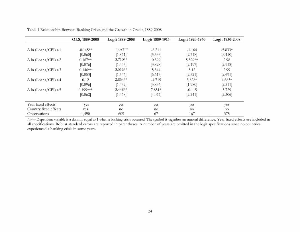
Table 1 presents results for the models and sub-samples. Overall there is a strong positive

relationship between real credit growth and the probability of having a banking crisis. Although real

credit growth lagged one year is associated with a lower probability of a crisis, credit growth from

two to five years earlier is strongly positively related to a crisis. The sum of lag coefficients in

column 1 is 0.487. In the linear probability model, the sum of coefficients implies that a sustained

five year period rise of one standard deviation or 0.10 log points in real bank loans would be

associated with a rise in the probability of a banking crisis of 0.049. The results are somewhat larger

if we use the logit specification from column 2. Here a rise in the growth of real credit from 0.05 to

0.15 (roughly one standard deviation above the mean) would raise the predicted probability by 0.15.

For the sample that is restricted to the post-World War II period, the impact is slightly smaller. Here

there is a rise in the probability of 0.06 when the mean growth of credit rises from its mean of 0.04

by one standard deviation to 0.10. These results are in line with Schularick and Taylor and the

literature on credit booms surveyed above. They pave the way to thinking about the fundamental

drivers of credit growth.

4. Credit Growth Determinants

In this section we explore the cross-country relationship between the growth in credit and

other macroeconomic aggregates. Our dependent variable is credit growth, and the set of

independent variables includes income concentration as well as some of the more traditional

variables included in Mendoza and Terrones and Borio and White.

12  

The goal here is to provide a simple econometric test of the hypothesis that credit growth

has no relationship to changes in income concentration after conditioning on other factors. The

alternative hypothesis, discussed above, is that income inequality or top income concentration drives

credit growth even after controlling for other macroeconomic variables. Again, there is strong

evidence, based on our priors and previous research, that there is a relationship between credit

growth and the business cycle and other macroeconomic aggregates. There is also some evidence

that changes in inequality are related to these cyclical variables. Whether changes in inequality matter

once we control for these variables is then a question for the data.

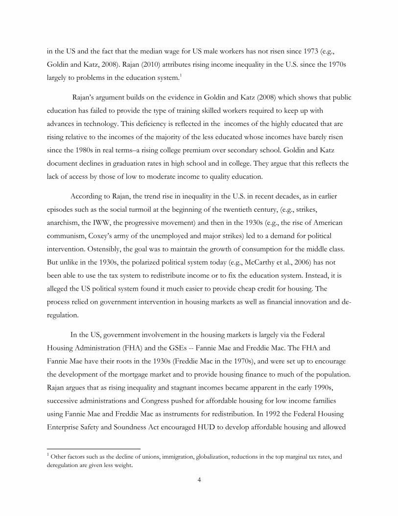
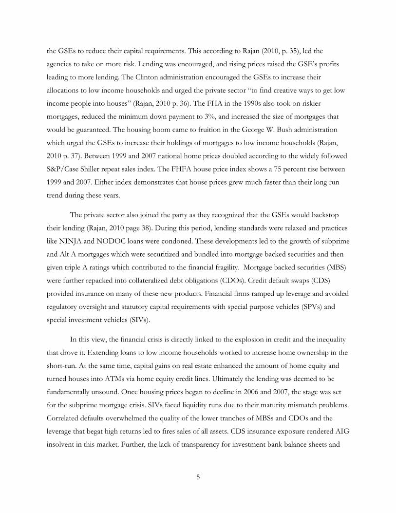
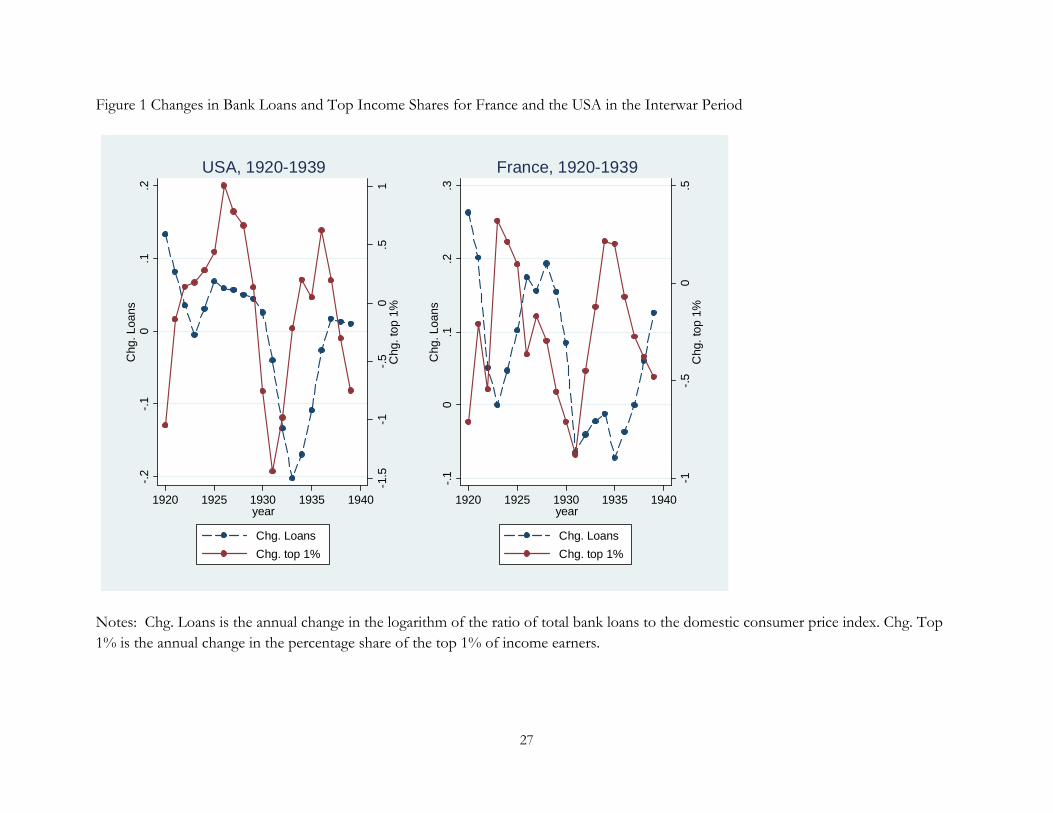
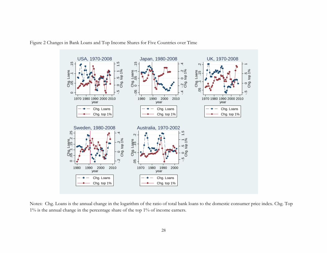
4.1 Time Series Plots of Credit and Top Incomes

Time series plots of the growth in credit (i.e., the change in the log ratio of bank loans to the

price index) and of changes in the share of income for the top 1% for seven different country/time

periods are presented in Figures 1 and 2. For the US, we look at the following periods: 1924-1929,

1993-2000 and 2004-2007. All three seem to be suggestive of a positive relationship between credit

growth and rises in top income shares. Of course, the economy was in full expansion during the

bulk of these periods, so that an alternative view might simply be that general economic expansion

generates these co-movements. There are only a limited number of examples from other countries

that support the idea that income concentration drives credit. Sweden from 2003-2008 might also be

consistent with the US case between 2004 and 2007.

Despite these examples, there are many cases that do not fit the RKR frameworks. In Japan

in the 1980s, credit growth clearly rises in advance of top income shares. On the other hand, top

income shares started rising in 1995 in Japan while credit growth languished. In Sweden, sharp rises

in top incomes followed, rather than led credit growth in the 1980s. Again, in Sweden, top income

shares continued to grow in the aftermath of the banking and real estate bust in 1991 while credit

fell. In Australia, credit growth was unrelated to top income shares in the 1970s. Top income shares

follow rather than lead credit growth in the late 1980s in Australia. The UK shows similar patterns

that do not fit the story that rising income concentration endogenously generates a credit boom.

13  

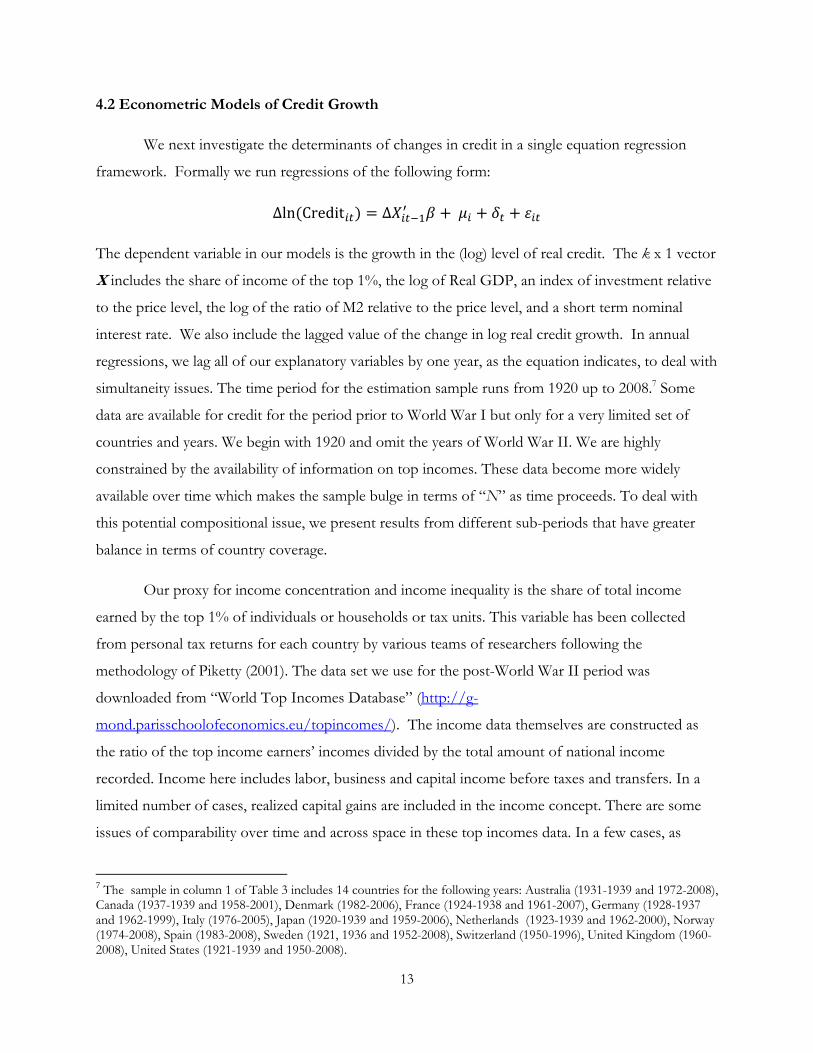
4.2 Econometric Models of Credit Growth

We next investigate the determinants of changes in credit in a single equation regression

framework. Formally we run regressions of the following form:

Δln Credit Δ

The dependent variable in our models is the growth in the (log) level of real credit. The k x 1 vector

X includes the share of income of the top 1%, the log of Real GDP, an index of investment relative

to the price level, the log of the ratio of M2 relative to the price level, and a short term nominal

interest rate. We also include the lagged value of the change in log real credit growth. In annual

regressions, we lag all of our explanatory variables by one year, as the equation indicates, to deal with

simultaneity issues. The time period for the estimation sample runs from 1920 up to 2008.7 Some

data are available for credit for the period prior to World War I but only for a very limited set of

countries and years. We begin with 1920 and omit the years of World War II. We are highly

constrained by the availability of information on top incomes. These data become more widely

available over time which makes the sample bulge in terms of “N” as time proceeds. To deal with

this potential compositional issue, we present results from different sub-periods that have greater

balance in terms of country coverage.

Our proxy for income concentration and income inequality is the share of total income

earned by the top 1% of individuals or households or tax units. This variable has been collected

from personal tax returns for each country by various teams of researchers following the

methodology of Piketty (2001). The data set we use for the post-World War II period was

downloaded from “World Top Incomes Database” (http://g-

mond.parisschoolofeconomics.eu/topincomes/). The income data themselves are constructed as

the ratio of the top income earners’ incomes divided by the total amount of national income

recorded. Income here includes labor, business and capital income before taxes and transfers. In a

limited number of cases, realized capital gains are included in the income concept. There are some

issues of comparability over time and across space in these top incomes data. In a few cases, as

                                                            7 The sample in column 1 of Table 3 includes 14 countries for the following years: Australia (1931-1939 and 1972-2008), Canada (1937-1939 and 1958-2001), Denmark (1982-2006), France (1924-1938 and 1961-2007), Germany (1928-1937 and 1962-1999), Italy (1976-2005), Japan (1920-1939 and 1959-2006), Netherlands (1923-1939 and 1962-2000), Norway (1974-2008), Spain (1983-2008), Sweden (1921, 1936 and 1952-2008), Switzerland (1950-1996), United Kingdom (1960-2008), United States (1921-1939 and 1950-2008).

14  

mentioned, capital gains are included in the income concept. The definition of the tax unit also

varies by country and over time. Some issues in comparability over time due to changes in tax laws

have also been highlighted by Piketty and Saez who provided the web-based interface for the World

Top Incomes Database. Despite these caveats, we follow Roine, Vlachos and Waldenström (2009)

and pool these data as a reasonable first pass at the key relationships.8

4.3 Credit Growth Determinants: Evidence from Five Year Periods

Our first results rely on information from five-year periods as in Roine et. al. Annual volatility is

significant in the data especially in the top income shares. Also this is an attempt to look at medium

term trend relationships which is the horizon on which the RKR frameworks seem to be focused.

An observation in this sample is thus the cumulative change over the previous five years for each

variable. We restrict the sample to the endpoint of each quinquenium, and period dummies are

included for each five year period to control for shocks. In these models, variables in the vector X

are for the same five-year period.

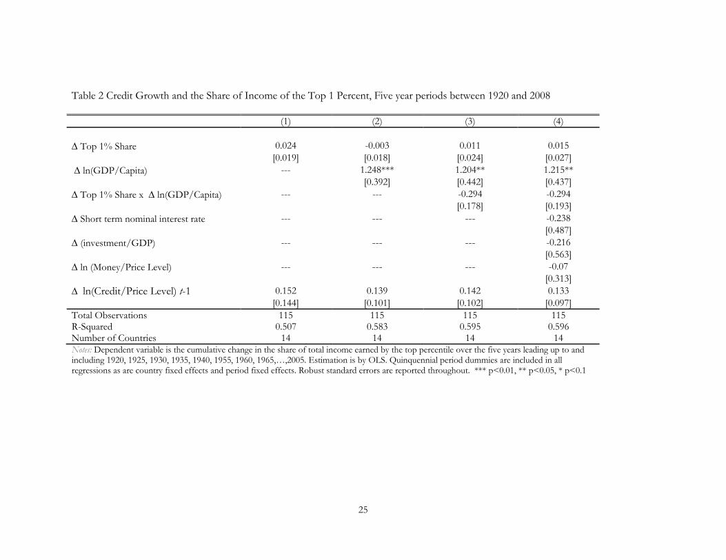
Table 2 presents four OLS regressions where the dependent variable is the cumulative growth

over the previous five-years in the log of real credit. Column 1 includes only the cumulative

percentage point change in the top income share as well as country fixed effects, time dummies, and

growth in credit from the previous five-year period. While top income growth has a positive

marginal effect, it is only significant at the 80 percent level of confidence. Column 2 adds the

cumulative change in the log of real GDP over the previous five years to the model in column 1.

Income growth is strongly related to credit growth. Again, we fail to reject the null hypothesis that

top incomes have no association with the growth in credit. In column 3, we interact these two key

variables. The reason is that the RKR hypothesis suggests that when total incomes and inequality are

rising a credit boom arises in the bid to smooth consumption by the lower deciles. We find no

evidence of such an impact with the interaction effect. Finally, column 4 controls for other

macroeconomic fundamentals including the short-term nominal interest rate, the ratio of investment

                                                            8 We note that income inequality measures based on the Gini Coefficient or comparisons between the 90th and the 10th or the 50th percentiles are different from the top incomes variable which captures only one part of the distribution. For checking the robustness of our results, we also investigated, but do not report results using the top 5% and the top 10% of earners.  

15  

to GDP and the (log) real money supply (M2). The only variable that has a statistically significant

relationship after inclusion of these controls is the growth of GDP.

From Table 2, the evidence is that the primary determinant of credit growth is real incomes.

When GDP grows at a pace above its average, credit also rises above its average growth rate. We

decisively reject any relationship between credit growth and changes in the share of income accruing

to the top 1%. In unreported regressions, we found that no relationship existed between credit

growth and the share of the top 0.01%, the top 5%, or the top 10%.

4.4 Credit Growth Determinants: Annual Evidence

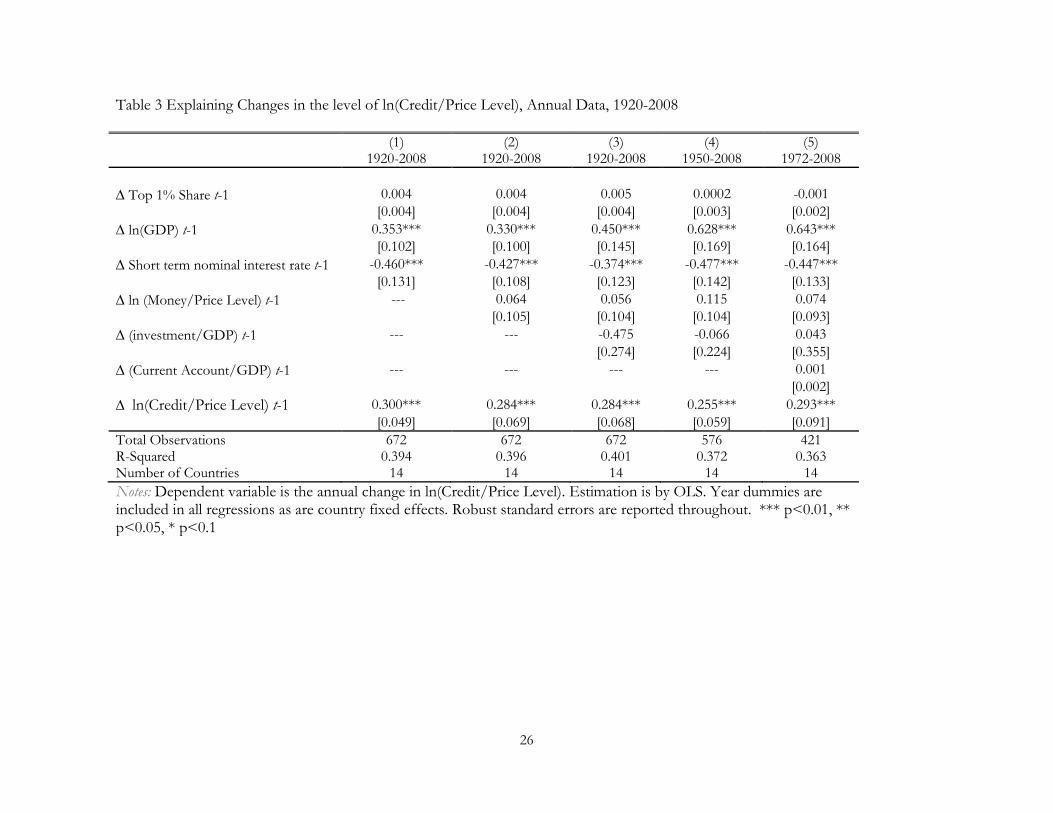
Table 3 examines the relationship between credit growth and these determinants using

annual data. Year-to-year variation provides another perspective and a robustness check on our

results from Table 2. Once again, the annual data provide no evidence that growth in top income

shares are a significant determinant of credit growth. In none of the specifications presented, or in

the many which we leave unreported, do top incomes have any statistically significant relationship

with credit growth. On the other hand, all specifications show a strong relationship between annual

changes in GDP and credit growth.

Table 3 also presents evidence from three different subsamples. The first three columns are

for the 1920-2008 period, the fourth column is limited to the years between 1950 and 2008, and the

fifth column is for 1972-2008 when international capital flows began to rise rapidly. The first three

columns add progressively more explanatory variables to the long-run sample. Echoing results in

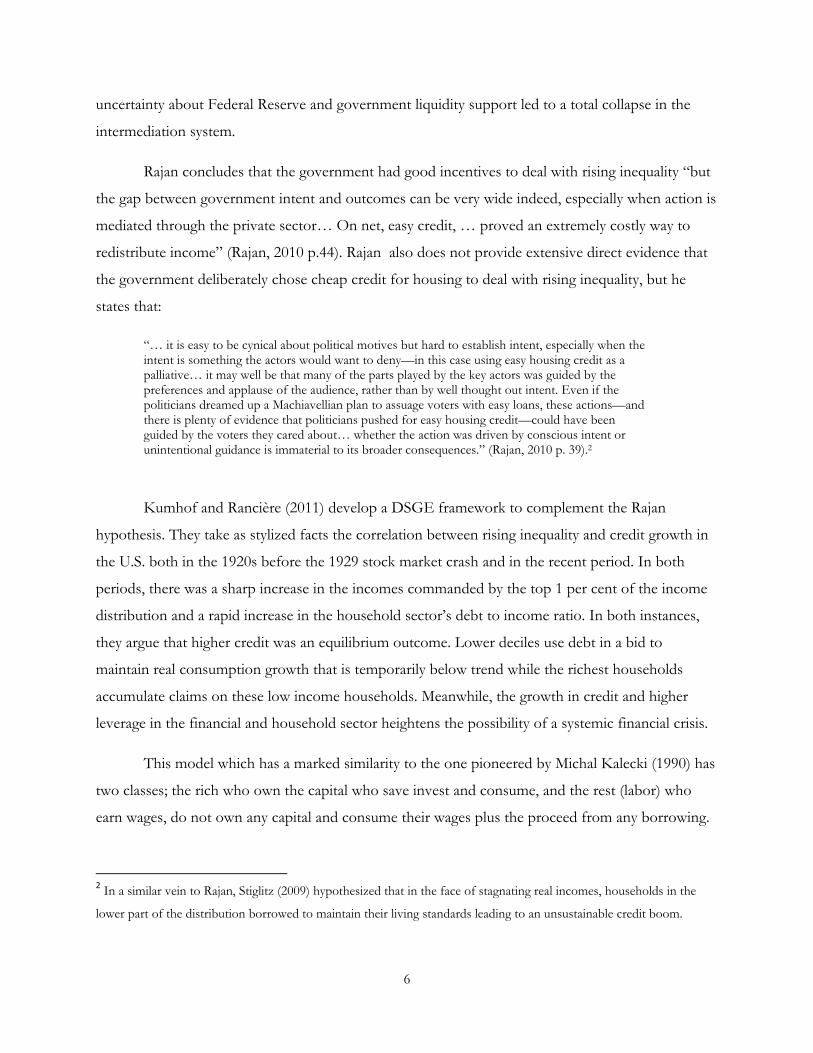
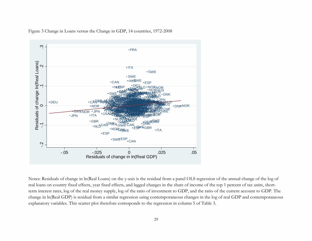
Table 2, GDP growth is highly significant and positively related to credit growth. Figure 3 presents

this relationship in a scatter plot. This figure plots the relationship between residuals from

regressions of credit growth and income growth that condition on country and time fixed effects

and all variables included in column 4 of Table 3. Here one gets a sense of how tight the conditional

relationship is between changes in top incomes and changes in income growth. Given the standard

error of the estimated relationship, there is less than a 1 in 1000 chance that this relationship is

statistically indistinguishable from zero, while the 95% confidence band is 0.25 to 1.03.

Table 3 shows that changes in the short-term nominal interest rate are also a significant

determinant of credit growth. When short-term interest rates fall, credit growth rises. This result is

16  

also robust to using ex post real interest rates. The relation between interest rates and credit seems

to be consistent with the Borio and White story that low interest rates reflecting benign inflationary

expectations can provide an environment favorable to creating a credit boom. It is also consistent

with a simpler story emphasizing the role of loose monetary policy in fueling a credit boom. This

result, together with the relationship between credit and income growth resoundingly rejects any role

for income concentration.

The negative relationship between interest rates and credit might also be consistent with a

“savings glut” type of argument. An increase in the supply of savings drives interest rates down

perhaps due to rising savings abroad or in the upper deciles. If the upper deciles were responsible

for this rise, then it might be consistent with RKR. If so, then the top income share and interest

rates should be strongly negatively correlated. There is no strong evidence for this notion. When we

omit interest rates from column 1, the coefficient on top incomes rises to 0.0046 from 0.0042. The

standard error hardly changes either.

As a robustness check, three other variables were included in Table 3: money growth,

changes in the rate of investment relative to GDP and changes in the current account to GDP ratio.

Mendoza and Terrones (2008) found that a rise in the current account deficit accompanied credit

booms, but their sample included many emerging markets as well as leading countries. Our sample is

limited to a subsample of the most developed countries. Here current account deficits have no

significant relationship with credit growth.

A long literature on credit booms argues that technological breakthroughs and displacements

drive investment and these need to be financed with credit (Fisher 1933, Kindleberger 1978, Minsky

1986). After controlling for the business cycle and the interest rate, we find no convincing evidence

that higher investment is associated with credit growth. Money supply growth is also not associated

with credit growth. This result is consistent with Schularick and Taylor (forthcoming) who observe a

dwindling correlation between growth in the money supply and bank lending since World War II.

According to them, this reflected financial innovation allowing banks to increase leverage and rely

less on deposits for their funding. Overall, low interest rates and strong economic growth seem to

be the most robust determinants of credit growth.

None of the econometric models we have deployed can reject the null hypothesis that top

income shares have no relationship with changes in credit. Our cross-country evidence is also

17  

inconsistent with Kumhof and Rancière who argued that rises in inequality could give rise to credit

booms and financial crises. The results in Table 1 show a high probability of a banking crisis after

credit growth rises, but since top income growth is not a determinant of credit growth, income

concentration is not associated with banking crises. Indeed, unreported regressions that include

growth in top incomes in regressions like those of Table 1 show that income inequality is not a

significant determinant of banking crises in our sample.

5. Historical Evidence & Discussion

Recent literature has made the novel claim that income inequality in the US played a big role

in driving the credit boom from 2002 and in the 1920s. Our cross country empirical evidence shows

that there is no statistical relationship between income concentration and credit booms. In fact,

historical evidence from the episodes in the US which are used to motivate RKR shows that income

concentration may be only coincidental with these credit boom and bust episodes. Here we provide

some anecdotal evidence in support of our findings above.

For the 1920s, time series for the US show that the share of income earned by the top 1%

increased from 15% in 1922 to 18.42% in 1929. Research based on top-incomes, as well as early

work by Williamson and Lindert (1980), identify this as a period of rising income inequality.

However, this rise in income inequality does not seem to be associated with any stagnation in real

wages for the working class. Indeed annual income of nonfarm employees rose grew at an average

of 1.89 percent or a total of 23 percent between 1919 and 1929. In addition, rises in the standard of

living must have been even greater. Leisure increased in this period as the standard work week fell to

48 hours by 1929. The introduction of electrification, better indoor plumbing and a host of new

consumer durables including automobiles, radio, washing machines and refrigerators, made home

production more efficient and leisure more enjoyable.

At the same time, as credit allegedly “boomed” in the 1920s, the economy grew largely

above trend from 1923 up to 1929. Olney (1999) reports that consumer non-mortgage debt to

income rose from 5.6% to 9.3% between 1923 and 1929. The ratio of individual and non-corporate

debt to nominal income (this includes farm production credit, farm mortgages, non-farm mortgages,

commercial, financial and consumer credit) increased between 1923 and 1929 from 63% ($53.7

18  

billion in credit and $85.1 billion in gross output) to 70.7% ($72.9 billion in credit versus $103.1

billion in gross output).9 The bulk of the rise in credit was attributable to non-farm mortgage lending

which rose by $13.3 billion. Consumer credit doubled from $3.2 billion to $6.4 billion in nominal

terms between 1923 and 1930 but the amounts were relatively small relative to total income.

Eichengreen and Mitchener (2004) cite competition amongst lenders, monetary stability and

improved housing quality as drivers of the housing boom.

Eugene N. White (2009) delves further into the US housing boom of 1920-1926

investigating demand, monetary policy, lending standards, mortgage securitization, risk-taking and

supervision. Out of sample predictions of a demand for housing model account for a large portion

of the rise in housing starts since demand had been repressed during the war, GDP was growing fast

and interest rates were low. Still, the portion of housing starts left unexplained by this model is equal

to ½ to 2/3 of annual average housing starts from 1900-1917. White concludes that monetary policy

was somewhat too loose, but other important features of the boom were supply-side financial

innovations including mortgage securitization, weakened supervision of lenders, lower lending

standards and even corruption. White recounts that Florida politicians were “bought” by developers

in order to achieve low supervision and easy charters. This version of the story is driven by the

supply side rather than the demand side as in RKR. White is also emphatic that the housing bust did

not impair the financial system or generate a banking crisis in 1926 nor was the housing boom and

bust directly responsible for the banking crises of 1930, 1931-32 and 1933. There is little evidence

that housing, which accounts for the bulk of the rise in household borrowing in the 1920s, was

affected by the level of earnings inequality in the period.

Consumer credit was closely related to the rise of new big-ticket consumer durables in the

1920s. However, the rise in consumer credit also arguably came from supply side innovations rather

than from a household demand to maintain consumption in the face of stagnant incomes. The

historical record is not consistent with the RKR hypothesis in this regard. Olney (1989)

demonstrates that a major driver of consumer credit for automobiles, an important component of

overall consumer credit, was pressure from automobile manufacturers. Producers wanted retailers to

carry the costs of the winter inventory buildup so that production could be smoothed and average

costs could be lower. The solution was the advent of finance companies including GMAC that

                                                            9 While nominal credit aggregates peaked in 1929, the ratio of debt to GDP continued to grow up to 1933 due to the fact that nominal GDP declined by almost 50% between 1929 and 1933.

19  

innovated methods of extending credit to consumers. Often they did so by purchasing installment

contracts from dealers. The original intent was not to “bolster retail sales but to finance dealer’s

wholesale inventory” (Olney, 1989).

On this basis it is very hard to generalize the RKR view even to the 1920s in the United

States. There is simply no evidence of a political conspiracy to increase home-owning in the 1920s in

the USA in order to win votes. Nor is there any evidence that the demand for credit rose in order to

make up for lost income and lagging consumption. Eichengreen and Mitchener (2004) dissect the

1920s credit boom and suggest that the view of Borio and White is largely consistent with the cross-

country experience. In the US, but also in other nations, competition in the financial sector and

accommodative monetary policy in the 1920s drove credit up during the boom and likely fed back

into the economic cycle. The stock market crash in 1929 and the subsequent economic slump can be

attributed to many causes but amongst them are the large financial imbalances that built up over the

1920s which were cataclysmic for household balance sheets and aggregate demand due to the

subsequent deflation (Mishkin, 1978 Olney, 1999).

The experience of other countries that experienced major credit booms and subsequent

financial crises is also not obviously consistent with RKR. Sweden had a credit boom following the

liberalization of their financial sector in the 1980s. The other key factors leading to its systemic

banking crisis in 1991 were capital inflows and an overvalued exchange rate (Jonung et. al. 2009).

Australia had a massive housing and credit boom in the late 1980s as well. Factors cited there were

rapid financial de-regulation, excessive risk taking in the corporate sector and irrational speculation

in the housing market (Macfarlane, 2006). Japan’s real estate boom in the 1980s was also fueled by

expansionary monetary policy under pressure from the U.S. to weaken the Yen at the Plaza Accord

of 1985 (Funibashi, 1989). Mullbauer and Murphy (1990) argued that the UK credit and

consumption boom of the late 1980s was enabled by financial liberalization that allowed consumers

to cash in on housing equity. An alternative story for the UK in the 1980s is that households

anticipated an increase in lifetime labor incomes (Attanasio and Weber, 1994). None of these cases

or points of view associates the credit and asset price booms with rising income inequality. Most of

them witnessed declining interest rates or accommodative monetary policy, financial liberalization

and economic expansion.

20  

6. Conclusions

Our paper looks for empirical evidence that might corroborate Rajan (2010) and Kumhof

and Rancière (2011). Both attributed the US subprime crisis to rising inequality, redistributive

government housing policy and a credit boom. Using data from a panel of 14 countries for over 120

years, we find strong evidence linking credit booms to banking crises, but no evidence that rising

income concentration was a significant determinant of credit booms. Narrative evidence on the US

experience in the 1920s, and that of other countries in more recent decades, casts further doubt on

the role of rising inequality.

We do find significant evidence that rising real income and falling interest rates are

important determinants of credit booms. This evidence is more consistent with the alternative story

of Borio and White (2003) attributing credit booms and crises in the past three decades to the Great

Moderation which created a benign environment conducive to rising credit. It is also consistent with

other empirical work that covers the period 1960-2002 (Mendoza and Terrones, 2008). The negative

and significant relationship of short-term interest rates and credit growth may also be consistent

with the story of for example Taylor (2009) or Meltzer (2010) who attribute the U.S. housing boom

to expansionary policy by the Federal Reserve in the early 2000s in an attempt to prevent perceived

deflation. Moreover, housing booms and busts in other countries did not reflect redistributive

housing policy. In the period before the Great Moderation they occurred during episodes of

expansionary monetary policy. Regardless of whether the Borio and White story or a simpler

monetary policy story is the true explanation for credit booms that lead to financial crises it now

seems fairly clear from our examination of the data that neither have much to do with rising income

inequality.

21  

References

Attanasio, O. Weber, G. 1994. UK Consumption Boom of the Late 1980s: Aggregate Implications

of Microeconomic Evidence. Economic Journal 104 (427) pp. 1269-1302.

Atkinson, A.B., Piketty, T., Saez, E. 2011 Top Incomes in the Long Run of History. Journal of

Economic Literature. 49 (1) 3-71.

Atkinson, T., Morelli, S. 2010. Inequality and Banking Crises: A First Look. mimeo, Oxford

University.

Barlevy, G. Tsiddon, D. 2006 Earnings inequality and the business cycle. European Economic

Review. 50 pp. 55-89.

Bernanke,B and Gertler M, 2000. Monetary Policy and Asset Price Volatility. American Economic

Review. May

Bordo, M. and Jeanne, O. 2002. Monetary Policy and Asset prices: Does Benign Neglect Make

Sense? International Finance.

Bordo, M. Eichengreen, B, Klingebiel, D., Martinez-Peria, M.S. 2001. “Is the Crisis Problem

Growing More Severe?” Economic Policy, 16 (32), 53-82.

Borio, C., Lowe, P. 2002. Asset prices, financial and monetary stability: exploring the nexus. BIS

Working Papers. no 114.

Borio, C. and White, W. W. 2003. Whither monetary and financial stability? The implications of evolving policy regimes. in Monetary Policy and Uncertainty: Adapting to a Changing Economy: A Symposium sponsored by the Federal Reserve Bank of Kansas City, Jackson Hole, Wyoming, 28-30 August, pp 131-211.

Eichengreen, B., Mitchener, K. 2004. The Great Depression as a Credit Boom Gone Wrong.” Research in Economic History. 22.

Fisher, I. 1933 “The Debt Deflation Theory of Great Depressions.” Econometrica 1 (4). Pp. 337-357.

Funibashi, Y. 1988. Managing the Dollar: From the Plaza to the Louvre. Institute for International Economics. Washington DC

22  

Goldin, C. Katz, L. 2008. The Race Between Education and Technology. Belknap Press.

Jonung, L. Kiander, J and Vartia, P. 2009. The Great Financial Crisis in Finland and Sweden: The

Nordic Experience of Financial Liberalization. London. Edward Elgar

Kalecki, M. 1990-1997.Collected Works of Michal Kalecki, 7 vols, ed. J. Osiatynski. Oxford:

Clarendon.

Kindleberger, C. 1996. Manias , Panics and Crashes: A History of Financial Crises. New York: John

Wiley

Kumhof, M., Rancière, R. 2011. Inequality, Leverage and Crises IMF working Paper 10/268.

McCarthy, N, Poole, K and Rosenthal, H. 2006. Polarized America: The Dance of Ideology and

Unequal Risks. Cambridge MA ; MIT Press

Macfarlane, I. 2006. The Search for Stability. Australian Broadcasting Company Boyer Lectures.

Mendoza, E.G. Terrones, M. 2008. An Anatomy of Credit Booms: Evidence from the Macro

Aggregates and Micro Data. NBER Working Paper 14049.

Minsky, H. 1986. Stabilizing an Unstable Economy. New Haven: Yale University Press

Mishkin, F., 1978. The household balance sheet and the Great Depression. Journal of Economic

History 38, 918--937.

Mullbauer, J., Murphy, A. 1990. Is the UK balance of payments sustainable?. Economic Policy. 11

pp. 345-83.

Olney, M. 1999. Avoiding Default: The Role of Credit in the Consumption Collapse Of 1930.

Quarterly Journal of Economics, 114 (1), 319-335.

Olney, M. 1989. Credit as a Production-Smoothing Device: The Case of Automobiles, 1913-1938

Journal of Economic History. 49 (2). Pp. 377-391.

Piketty, Thomas, 2001a. Les hauts revenus en France au 20ème siècle. Grasset, Paris.

Rajan, R. 2010. “Fault Lines” Princeton University Press, Princeton, NJ.

23  

Roine, J. Vlachos, J., Waldenström, D. 2009. The long-run determinants of inequality: What can we

learn from top income data? Journal of Public Economics 93. 974-988.

Schularick, M. and Taylor A.M. forthcoming. Credit Booms Gone Bust Monetary Policy, Leverage

Cycles and Financial Crises, 1870–2008. American Economic Review.

Stiglitz, J 2009. “Joseph Stiglitz and Why Inequality is at the Root of the Recession” Next Left

website. January 9 2009.

Taylor, J.B., 2009. Getting Off Track: How Government Actions and Intervention Caused,

Prolonged and Worsened the Financial Crisis. Stanford. Hoover Institution Press.

White, Eugene N. 2009. Lessons from the Great American Real Estate Boom and Bust of the

1920s. NBER Working Paper No. 15573.

Williamson, J.G., Lindert, P.H. 1980. American Inequality: A Macroeconomic History. Academic

Press Inc, New York.

 

24  

Table 1 Relationship Between Banking Crises and the Growth in Credit, 1889-2008

OLS, 1889-2008 Logit 1889-2008 Logit 1889-1913 Logit 1920-1940 Logit 1950-2008 ln (Loans/CPI) t-1 -0.145** -4.087** -6.211 -1.164 -5.833* [0.060] [1.861] [5.533] [2.718] [3.410] ln (Loans/CPI) t-2 0.167** 3.710** 0.399 5.329** 2.98 [0.076] [1.445] [3.828] [2.197] [2.918] ln (Loans/CPI) t-3 0.146** 3.316** 5.344 3.12 2.99 [0.053] [1.546] [6.613] [2.521] [2.691] ln (Loans/CPI) t-4 0.12 2.854** -4.719 3.828* 4.685* [0.096] [1.432] [3.836] [1.980] [2.511] ln (Loans/CPI) t-5 0.199*** 3.448** 7.851* -0.115 3.729 [0.062] [1.468] [4.077] [2.241] [2.306] Year fixed effects yes yes yes yes yes Country fixed effects yes no no no no Observations 1,490 609 67 167 375 Notes: Dependent variable is a dummy equal to 1 when a banking crisis occurred. The symbol signifies an annual difference. Year fixed effects are included in all specifications. Robust standard errors are reported in parentheses. A number of years are omitted in the logit specifications since no countries experienced a banking crisis in some years.

25  

Table 2 Credit Growth and the Share of Income of the Top 1 Percent, Five year periods between 1920 and 2008 (1) (2) (3) (4) Top 1% Share 0.024 -0.003 0.011 0.015 [0.019] [0.018] [0.024] [0.027] ln(GDP/Capita) --- 1.248*** 1.204** 1.215** [0.392] [0.442] [0.437] Top 1% Share x ln(GDP/Capita) --- --- -0.294 -0.294 [0.178] [0.193] Short term nominal interest rate --- --- --- -0.238 [0.487] (investment/GDP) --- --- --- -0.216 [0.563] ln (Money/Price Level) --- --- --- -0.07 [0.313] ln(Credit/Price Level) t-1 0.152 0.139 0.142 0.133 [0.144] [0.101] [0.102] [0.097] Total Observations 115 115 115 115 R-Squared 0.507 0.583 0.595 0.596 Number of Countries 14 14 14 14 Notes: Dependent variable is the cumulative change in the share of total income earned by the top percentile over the five years leading up to and including 1920, 1925, 1930, 1935, 1940, 1955, 1960, 1965,…,2005. Estimation is by OLS. Quinquennial period dummies are included in all regressions as are country fixed effects and period fixed effects. Robust standard errors are reported throughout. *** p<0.01, ** p<0.05, * p<0.1

26  

Table 3 Explaining Changes in the level of ln(Credit/Price Level), Annual Data, 1920-2008

Notes: Dependent variable is the annual change in ln(Credit/Price Level). Estimation is by OLS. Year dummies are included in all regressions as are country fixed effects. Robust standard errors are reported throughout. *** p<0.01, ** p<0.05, * p<0.1

(1)1920-2008

(2)1920-2008

(3) 1920-2008

(4)1950-2008

(5)1972-2008

Top 1% Share t-1 0.004 0.004 0.005 0.0002 -0.001 [0.004] [0.004] [0.004] [0.003] [0.002] ln(GDP) t-1 0.353*** 0.330*** 0.450*** 0.628*** 0.643*** [0.102] [0.100] [0.145] [0.169] [0.164] Short term nominal interest rate t-1 -0.460*** -0.427*** -0.374*** -0.477*** -0.447*** [0.131] [0.108] [0.123] [0.142] [0.133] ln (Money/Price Level) t-1 --- 0.064 0.056 0.115 0.074 [0.105] [0.104] [0.104] [0.093] (investment/GDP) t-1 --- --- -0.475 -0.066 0.043 [0.274] [0.224] [0.355] (Current Account/GDP) t-1 --- --- --- --- 0.001 [0.002] ln(Credit/Price Level) t-1 0.300*** 0.284*** 0.284*** 0.255*** 0.293*** [0.049] [0.069] [0.068] [0.059] [0.091]Total Observations 672 672 672 576 421R-Squared 0.394 0.396 0.401 0.372 0.363Number of Countries 14 14 14 14 14

27  

Figure 1 Changes in Bank Loans and Top Income Shares for France and the USA in the Interwar Period

Notes: Chg. Loans is the annual change in the logarithm of the ratio of total bank loans to the domestic consumer price index. Chg. Top 1% is the annual change in the percentage share of the top 1% of income earners.

-1.5

-1-.5

0.5

1C

hg. t

op 1

%

-.2-.1

0.1

.2C

hg. L

oans

1920 1925 1930 1935 1940year

Chg. LoansChg. top 1%

USA, 1920-1939

-1-.5

0.5

Chg

. top

1%

-.10

.1.2

.3C

hg. L

oans

1920 1925 1930 1935 1940year

Chg. LoansChg. top 1%

France, 1920-1939

28  

Figure 2 Changes in Bank Loans and Top Income Shares for Five Countries over Time

Notes: Chg. Loans is the annual change in the logarithm of the ratio of total bank loans to the domestic consumer price index. Chg. Top 1% is the annual change in the percentage share of the top 1% of income earners.

-.50

.51

1.5

Chg

. top

1%

0.0

5.1

.15

Chg

. Loa

ns

1970 1980 1990 2000 2010year

Chg. LoansChg. top 1%

USA, 1970-2008

-.4-.2

0.2

.4C

hg. t

op 1

%

-.05

0.0

5.1

.15

Chg

. Loa

ns

1980 1990 2000 2010year

Chg. LoansChg. top 1%

Japan, 1980-2008

-.50

.51

Chg

. top

1%

.05

.1.1

5.2

Chg

. Loa

ns

1970 1980 1990 2000 2010year

Chg. LoansChg. top 1%

UK, 1970-2008

-.20

.2.4

Chg

. top

1%

0.0

5.1

.15

.2.2

5C

hg. L

oans

1980 1990 2000 2010year

Chg. LoansChg. top 1%

Sweden, 1980-2008

-.50

.51

1.5

Chg

. top

1%

.05

.1.1

5.2

Chg

. Loa

ns

1970 1980 1990 2000year

Chg. LoansChg. top 1%

Australia, 1970-2002

29  

Figure 3 Change in Loans versus the Change in GDP, 14 countries, 1972-2008

 

 

 

 

 

 

 

 

 

 

 

 

 

Notes: Residuals of change in ln(Real Loans) on the y-axis is the residual from a panel OLS regression of the annual change of the log of real loans on country fixed effects, year fixed effects, and lagged changes in the share of income of the top 1 percent of tax units, short-term interest rates, log of the real money supply, log of the ratio of investment to GDP, and the ratio of the current account to GDP. The change in ln(Real GDP) is residual from a similar regression using contemporaneous changes in the log of real GDP and contemporaneous explanatory variables. This scatter plot therefore corresponds to the regression in column 5 of Table 3.

AUS

AUSAUS AUS

AUS

AUS

AUS

AUS

AUS

AUSAUS

AUSAUS

AUS

AUS

AUS

AUS

AUS

AUS AUS

AUS

AUS

AUS

AUSAUSAUS

AUSAUS

AUS

AUS

AUS

AUS

AUSAUS AUS

AUSAUS

CANCAN

CAN

CAN

CANCAN

CAN

CAN

CAN

CAN

CAN

CAN

CANCAN

CAN

CAN

CANCAN

CANCANCAN

CANCAN

CAN

CANCAN

CAN

CAN

CANCAN

DNK

DNK

DNK

DNK

DNK

DNK

DNK

DNKDNK

DNK

DNK

DNK

DNK

DNKDNKDNK

DNK

DNK

DNK

DNK

DNK

DNK

DNK

DNKDNK

FRAFRAFRA

FRA

FRA

FRA

FRA

FRA

FRA FRA

FRAFRA FRA

FRA

FRAFRA

FRA

FRA

FRA

FRA

FRAFRA

FRAFRAFRAFRAFRAFRA

FRA

FRAFRA

DEU

DEU

DEU

DEUDEUDEU

DEUDEU

DEUDEU

DEU

DEUDEUDEUDEUDEU DEU

DEU

DEU DEUDEUDEU

DEUDEUDEU

DEUDEU

ITA ITA

ITAITA ITA

ITA

ITA ITA

ITA

ITA

ITAITA

ITA

ITA

ITAITAITA

ITA

ITA

ITA

ITA

ITAITA

ITAITAITA

ITA

JPNJPN

JPN

JPNJPN

JPNJPNJPN

JPN

JPNJPNJPNJPNJPN

JPNJPNJPN

JPNJPNJPN

JPNJPN JPN

JPNJPN JPNJPNJPN NLD

NLD

NLDNLD

NLDNLD

NLD

NLDNLD

NLDNLD

NLD

NLDNLD

NLD

NLD

NLD

NLD

NLDNLDNLD

NLD

NLDNLD

NLD

NLD

NLD

NLDNLD

NOR

NOR

NOR

NORNORNOR

NOR

NORNORNOR

NOR

NOR

NOR

NOR

NOR

NOR

NOR

NORNOR

NOR

NOR

NORNORNOR

NORNOR

NOR

NOR

NOR

NOR NORNOR

ESP

ESP

ESP

ESP

ESP ESP

ESP

ESP

ESP

ESP

ESP

ESP

ESPESP

ESPESP ESP

ESP

ESPESP

ESPESP

ESP

ESPESP

ESPSWE

SWE

SWE

SWESWE

SWE

SWE

SWE

SWE

SWE

SWE

SWE

SWE

SWE

SWE

SWE

SWE

SWE

SWE

SWE

SWE

SWE

SWE

SWE

SWE

SWE

SWE

SWE

SWE

SWE

SWE

SWE

SWE SWESWE

SWESWE

CHE

CHE

CHE

CHE

CHECHE

CHE

CHE

CHE

CHE CHE

CHE

CHE

CHECHECHE

CHE

CHE

GBR

GBR

GBR

GBR

GBR

GBR

GBRGBRGBR

GBRGBR

GBRGBR

GBR

GBR

GBR

GBR

GBR

GBRGBR

GBR GBRGBRGBR

GBRGBR

GBRGBRGBRGBR

GBRGBR

GBR

GBRGBRGBRGBR

USAUSA

USAUSA

USA

USAUSA

USAUSA

USA USAUSA USA

USAUSAUSA

USAUSAUSAUSAUSA

USA

USAUSA

USA

USAUSA

USA

USA

USA

USA USAUSAUSAUSA

USA

USA

-.2-.1

0.1

.2.3

Res

idua

ls o

f cha

nge

ln(R

eal L

oans

)

-.05 -.025 0 .025 .05Residuals of change in ln(Real GDP)