Does Financial Market Structure Impact the Cost of Raising

Capital?

James Brugler, Carole Comerton-Forde and Terrence Hendershott*

February 1, 2018

Abstract

We examine the impact of secondary market structure and liquidity on the cost of raising capital.

In the 1990s trading on Nasdaq transformed from a dealer-oriented over-the-counter market to

a market where investors could directly interact with each other. The Order Handling Rules

(OHR) reforms that accomplished this were phased in across Nasdaq stocks over time allowing

for identification of their impact on firms’ cost of capital. We find that OHR significantly

reduced the underpricing of seasoned equity offerings by one to two percentage points from a

pre-OHR average of 3.6 percent. Using the staggered introduction of the OHR as an instrument

shows improved secondary market liquidity drives the reduction in underpricing.

* Brugler is at the Department of Finance, University of Melbourne. Comerton-Forde is at the School of Banking

and Finance at the UNSW Business School. Hendershott is at the Haas School of Business, University of California.

We thank Jeff Smith at Nasdaq for assistance in identifying and understanding the implementation of the Nasdaq

reforms. We also thank Frank Hatheway, Ross Levine, Dan Li, Joel Hasbrouck and participants at the FINRA and

Columbia University Market Structure Conference, the Australian National University Research Summer Camp and

the NBER Conference on Competition and the Industrial Organization of Securities Markets for helpful comments.

1

1 Introduction

Financial markets facilitate trading and price discovery by linking investors and firms. This impacts

firms’ cost of raising capital and, consequently, their investment decisions. The market structure

of trading affects secondary market liquidity (Madhavan, 2000). However, there is limited evidence

on how the structure of the secondary markets impacts the cost of raising capital in the primary

market through financing frictions. The cost of raising capital incorporates frictions in the issuing

process, such as the explicit fees and implicit costs related to underpricing at issuance.1 Our paper

provides direct, causal evidence on the relationship among the underpricing of seasoned equity

offerings (SEOs), market structure, and liquidity. Conducting such inference is complicated by a

number of sources of endogeneity between underpricing and liquidity.2

To estimate the effects of liquidity and market structure on SEO underpricing, we exploit a

significant change in the market structure of stocks trading on the Nasdaq in 1997, the Order

Handling Rules (OHR). These rules were designed to move Nasdaq from a dealer-oriented over-

the-counter (OTC) like structure to a more centralized order-driven market structure. The OHR

reforms were prompted by anti-competitive dealer behavior (Christie and Schultz, 1994). Two of

the most important components of these rules were that dealers were required to display limit

orders posted by members of public whenever these were at the best bid or offer and that dealers

were required to publicly display their best quotes, rather than on segmented marketplaces that

only certain types of investors could access.

Barclay et al. (1999), McInish, Van Ness, and Van Ness (1998), Weston (2000), and Chung

and Van Ness (2001) demonstrate that the OHR had the desired effect with quoted and effective

spreads declining by about one third. While depth at the best bid and offer also fell, Conrad et al.

1Corwin (2003), Butler, Grullon, and Weston (2005) and Ellul and Pagano (2006) examine underpricing and liquidity.Corwin (2003) estimates a positive but statistically weak association between bid-ask spreads and the underpricingof seasoned equity offerings. Butler, Grullon, and Weston (2005) show that stock liquidity is associated with lowerfees charged by investment banks for seasoned equity offerings. Ellul and Pagano (2006) find that the expected levelof liquidity and liquidity risk are determinants of IPO underpricing.

2A key reason why endogeneity is present in regressions of underpricing on liquidity is the presence of an unobservableomitted variable, such as information asymmetry, which can directly affect both underpricing (Rock, 1986; Beattyand Ritter, 1986; Carter and Manaster, 1990) and liquidity (Copeland and Galai, 1983; Glosten and Milgrom, 1985;Kyle, 1985). Uncertainty and information asymmetry can also cause sample selection bias, either through theircorrelation with firms’ financing needs or due to firms strategically timing their issues to minimize costs. In addition,high underpricing may itself be a signal for liquidity providers that investors are unwilling to take large positions ina given security and therefore may be indicative of inventory risk, implying simultaneity that would bias simple leastsquares regressions.

2

(2003) show that the OHR decreased the cost of executing large institutional orders by 5 to 15

basis points from a pre-OHR average cost of 40 to 50 basis points. Crucially for our purposes,

the OHR was specifically targeted at improving competition in market making on the Nasdaq. It

plausibly did not have a direct effect on underpricing. Hence, in addition to examining the effect

of the market structure change, we use the implementation of the rules as a source of exogenous

variation in liquidity. There are a number of other features of the OHR that are attractive for

our purposes. First, the rules were implemented in a staggered fashion, across 22 distinct dates

covering a 10 month period in 1997. Second, while the cohort of stocks included in a given wave

was determined by relative trading volume, there was a large degree of randomization within broad

categories of stocks. Third, by the end of the implementation period, all stocks listed on the Nasdaq

were covered by the rules implying that coverage went from zero to 100% in our sample period.

Fourth, the OHR only affected Nasdaq stocks so we can use New York Stock Exchange (NYSE)

stocks as controls.

While the staggered introduction provides treatment and control samples for within Nasdasq

study, the order of the stocks in the implementation of the OHR was not truly randomized. Stocks

with higher relative trading volume more likely to enter the program earlier. As such, our empirical

approach must be careful to distinguish between changes in liquidity that were due to the OHR

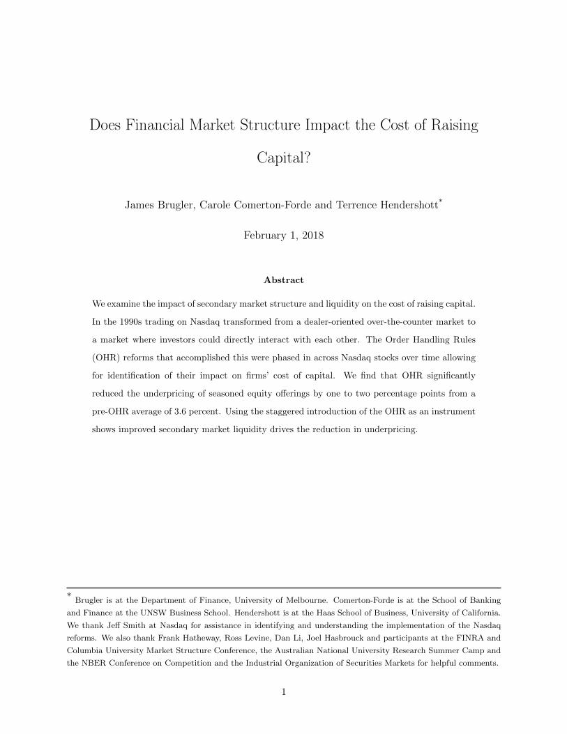
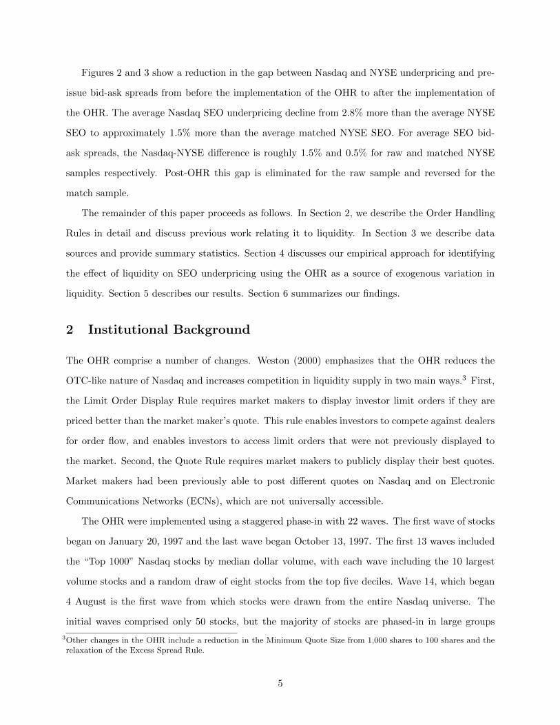
and those that were simply due to different characteristics across stocks in different phases. Figures

1a and 1b demonstrate this point. Underpricing and bid-ask spreads were both lower for stocks

completing SEOs after they were phased into the OHR. However, this may not reflect only a causal

effect of the OHR on liquidity and underpricing, but also systematic differences in characteristics

across OHR vs. non-OHR stocks.

Figure 1 about here

We use the OHR in several ways. First, we treat the OHR as a quasi-random experiment

and estimate its direct effect on SEO underpricing in a pooled difference-in-differences framework.

These regressions treat the OHR status as a dummy variable and estimate its effect both with and

without controls, stock-cohort fixed effects based on the date of inclusion in the OHR and time

fixed effects. By pooling our estimates across dates, we are able to get an estimate of the treatment

3

effect of the OHR without being so reliant on the parallel trends assumption as with only a single

treatment date (Bertrand and Mullainathan, 2003; Gormley and Matsa, 2011).

In our second approach, we use the OHR as an instrumental variable for liquidity in a re-

gression with SEO underpricing as the dependent variable. These regressions complement the

difference-in-differences regressions by allowing us to directly test whether any effect of OHR on

SEO underpricing was due to the influence that the new trading rules had on liquidity, rather than

through some other channel. These regressions also allow us to directly estimate the marginal

response of capital costs in the form of SEO underpricing to changes in market liquidity.

We find that the Order Handling Rules had a statistically and economically significant effect

of reducing SEO underpricing. In a difference-in-differences specification that includes cohort and

time fixed effects as well as stock and issue controls, SEOs of companies with stock trading under the

OHR were less underpriced by 2.18%, as compared to a 3.6% pre-OHR average SEO underpricing.

Our instrumental variable regressions confirm this result and show that improved secondary

market liquidity is the channel by which the OHR reduces underpricing. Using the variation

in liquidity that is driven by the OHR, we find that lower stock liquidity leads to higher SEO

underpricing. This effect is both statistically and economically significant. Further, the magnitude

of the effect estimated in these regressions is very similar to that estimated in the difference-in-

differences approach, when appropriately scaled. We interpret these results together as supportive

of the notion that the effect of the OHR on underpricing is due primarily to changes in liquidity,

and not due to some other factor that we have not controlled for.

In our third approach, to eliminate any concerns about non-random assignment in the rollout

schedule for OHR stocks we use NYSE stocks as controls to estimate the impact of the OHR on

SEO underpricing on Nasdaq. Because Nasdaq stocks are smaller and more volatile than NYSE

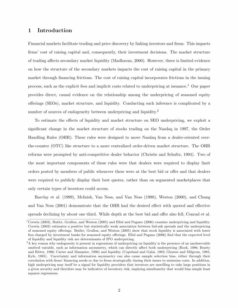
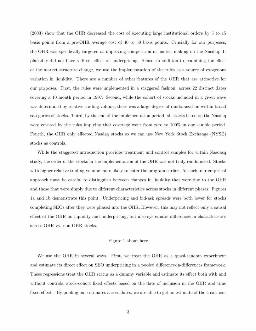
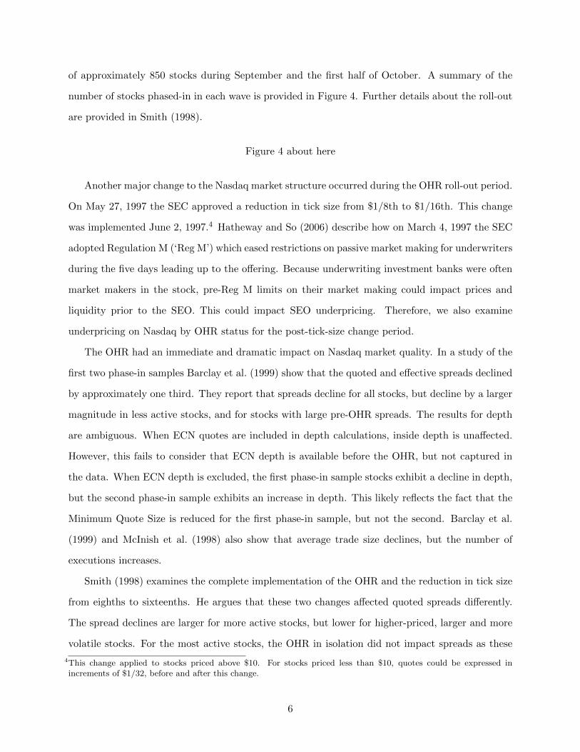
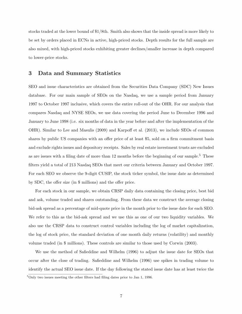
stocks we match SEOs across exchanges based on their issuers’ characteristics. Figures 2 and 3

plot the average underpricing and pre-issue bid-ask spread for Nasdaq and NYSE SEOs from June

1996 to June 1998. Panel (a) of these figures plots the means for all SEOs on both exchanges and

Panel (b) contains the mean for all Nasdaq SEOs and the mean for the matched sample of NYSE

SEOs where matching is conducted as per Section 4.3.

Figures 2 and 3 about here

4

Figures 2 and 3 show a reduction in the gap between Nasdaq and NYSE underpricing and pre-

issue bid-ask spreads from before the implementation of the OHR to after the implementation of

the OHR. The average Nasdaq SEO underpricing decline from 2.8% more than the average NYSE

SEO to approximately 1.5% more than the average matched NYSE SEO. For average SEO bid-

ask spreads, the Nasdaq-NYSE difference is roughly 1.5% and 0.5% for raw and matched NYSE

samples respectively. Post-OHR this gap is eliminated for the raw sample and reversed for the

match sample.

The remainder of this paper proceeds as follows. In Section 2, we describe the Order Handling

Rules in detail and discuss previous work relating it to liquidity. In Section 3 we describe data

sources and provide summary statistics. Section 4 discusses our empirical approach for identifying

the effect of liquidity on SEO underpricing using the OHR as a source of exogenous variation in

liquidity. Section 5 describes our results. Section 6 summarizes our findings.

2 Institutional Background

The OHR comprise a number of changes. Weston (2000) emphasizes that the OHR reduces the

OTC-like nature of Nasdaq and increases competition in liquidity supply in two main ways.3 First,

the Limit Order Display Rule requires market makers to display investor limit orders if they are

priced better than the market maker’s quote. This rule enables investors to compete against dealers

for order flow, and enables investors to access limit orders that were not previously displayed to

the market. Second, the Quote Rule requires market makers to publicly display their best quotes.

Market makers had been previously able to post different quotes on Nasdaq and on Electronic

Communications Networks (ECNs), which are not universally accessible.

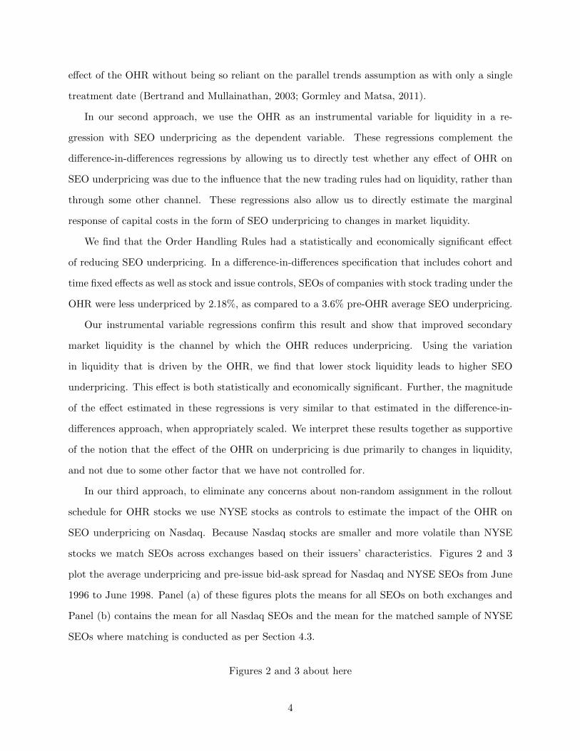
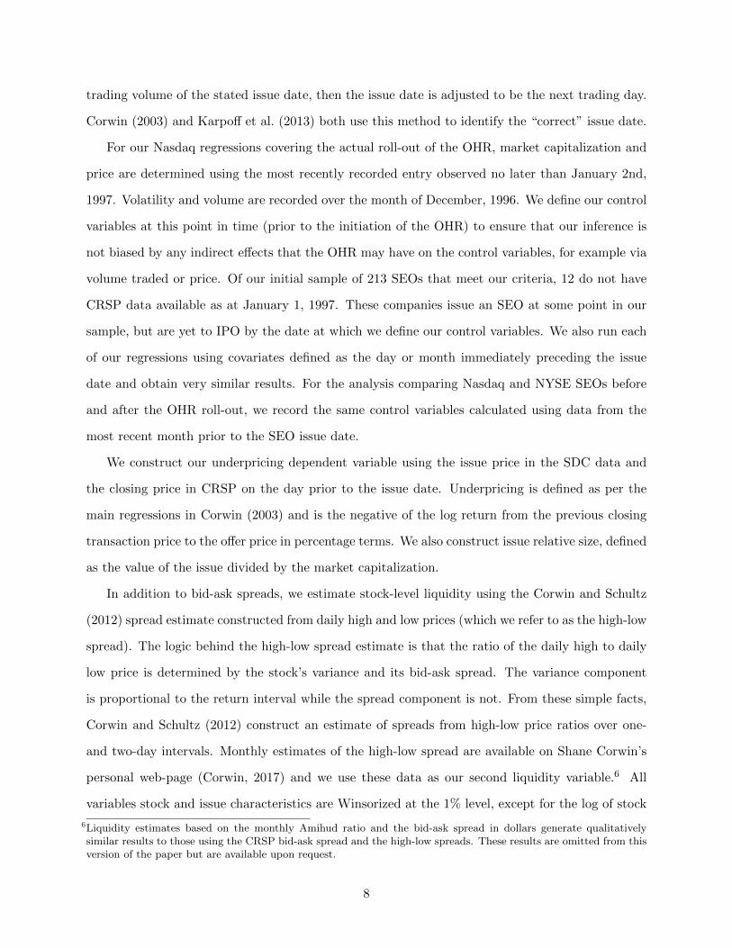
The OHR were implemented using a staggered phase-in with 22 waves. The first wave of stocks

began on January 20, 1997 and the last wave began October 13, 1997. The first 13 waves included

the “Top 1000” Nasdaq stocks by median dollar volume, with each wave including the 10 largest

volume stocks and a random draw of eight stocks from the top five deciles. Wave 14, which began

4 August is the first wave from which stocks were drawn from the entire Nasdaq universe. The

initial waves comprised only 50 stocks, but the majority of stocks are phased-in in large groups

3Other changes in the OHR include a reduction in the Minimum Quote Size from 1,000 shares to 100 shares and therelaxation of the Excess Spread Rule.

5

of approximately 850 stocks during September and the first half of October. A summary of the

number of stocks phased-in in each wave is provided in Figure 4. Further details about the roll-out

are provided in Smith (1998).

Figure 4 about here

Another major change to the Nasdaq market structure occurred during the OHR roll-out period.

On May 27, 1997 the SEC approved a reduction in tick size from $1/8th to $1/16th. This change

was implemented June 2, 1997.4 Hatheway and So (2006) describe how on March 4, 1997 the SEC

adopted Regulation M (‘Reg M’) which eased restrictions on passive market making for underwriters

during the five days leading up to the offering. Because underwriting investment banks were often

market makers in the stock, pre-Reg M limits on their market making could impact prices and

liquidity prior to the SEO. This could impact SEO underpricing. Therefore, we also examine

underpricing on Nasdaq by OHR status for the post-tick-size change period.

The OHR had an immediate and dramatic impact on Nasdaq market quality. In a study of the

first two phase-in samples Barclay et al. (1999) show that the quoted and effective spreads declined

by approximately one third. They report that spreads decline for all stocks, but decline by a larger

magnitude in less active stocks, and for stocks with large pre-OHR spreads. The results for depth

are ambiguous. When ECN quotes are included in depth calculations, inside depth is unaffected.

However, this fails to consider that ECN depth is available before the OHR, but not captured in

the data. When ECN depth is excluded, the first phase-in sample stocks exhibit a decline in depth,

but the second phase-in sample exhibits an increase in depth. This likely reflects the fact that the

Minimum Quote Size is reduced for the first phase-in sample, but not the second. Barclay et al.

(1999) and McInish et al. (1998) also show that average trade size declines, but the number of

executions increases.

Smith (1998) examines the complete implementation of the OHR and the reduction in tick size

from eighths to sixteenths. He argues that these two changes affected quoted spreads differently.

The spread declines are larger for more active stocks, but lower for higher-priced, larger and more

volatile stocks. For the most active stocks, the OHR in isolation did not impact spreads as these

4This change applied to stocks priced above $10. For stocks priced less than $10, quotes could be expressed inincrements of $1/32, before and after this change.

6

stocks traded at the lower bound of $1/8th. Smith also shows that the inside spread is more likely to

be set by orders placed in ECNs in active, high-priced stocks. Depth results for the full sample are

also mixed, with high-priced stocks exhibiting greater declines/smaller increase in depth compared

to lower-price stocks.

3 Data and Summary Statistics

SEO and issue characteristics are obtained from the Securities Data Company (SDC) New Issues

database. For our main sample of SEOs on the Nasdaq, we use a sample period from January

1997 to October 1997 inclusive, which covers the entire roll-out of the OHR. For our analysis that

compares Nasdaq and NYSE SEOs, we use data covering the period June to December 1996 and

January to June 1998 (i.e. six months of data in the year before and after the implementation of the

OHR). Similar to Lee and Masulis (2009) and Karpoff et al. (2013), we include SEOs of common

shares by public US companies with an offer price of at least $5, sold on a firm commitment basis

and exclude rights issues and depository receipts. Sales by real estate investment trusts are excluded

as are issues with a filing date of more than 12 months before the beginning of our sample.5 These

filters yield a total of 213 Nasdaq SEOs that meet our criteria between January and October 1997.

For each SEO we observe the 9-digit CUSIP, the stock ticker symbol, the issue date as determined

by SDC, the offer size (in $ millions) and the offer price.

For each stock in our sample, we obtain CRSP daily data containing the closing price, best bid

and ask, volume traded and shares outstanding. From these data we construct the average closing

bid-ask spread as a percentage of mid-quote price in the month prior to the issue date for each SEO.

We refer to this as the bid-ask spread and we use this as one of our two liquidity variables. We

also use the CRSP data to construct control variables including the log of market capitalization,

the log of stock price, the standard deviation of one month daily returns (volatility) and monthly

volume traded (in $ millions). These controls are similar to those used by Corwin (2003).

We use the method of Safieddine and Wilhelm (1996) to adjust the issue date for SEOs that

occur after the close of trading. Safieddine and Wilhelm (1996) use spikes in trading volume to

identify the actual SEO issue date. If the day following the stated issue date has at least twice the

5Only two issues meeting the other filters had filing dates prior to Jan 1, 1996.

7

trading volume of the stated issue date, then the issue date is adjusted to be the next trading day.

Corwin (2003) and Karpoff et al. (2013) both use this method to identify the “correct” issue date.

For our Nasdaq regressions covering the actual roll-out of the OHR, market capitalization and

price are determined using the most recently recorded entry observed no later than January 2nd,

1997. Volatility and volume are recorded over the month of December, 1996. We define our control

variables at this point in time (prior to the initiation of the OHR) to ensure that our inference is

not biased by any indirect effects that the OHR may have on the control variables, for example via

volume traded or price. Of our initial sample of 213 SEOs that meet our criteria, 12 do not have

CRSP data available as at January 1, 1997. These companies issue an SEO at some point in our

sample, but are yet to IPO by the date at which we define our control variables. We also run each

of our regressions using covariates defined as the day or month immediately preceding the issue

date and obtain very similar results. For the analysis comparing Nasdaq and NYSE SEOs before

and after the OHR roll-out, we record the same control variables calculated using data from the

most recent month prior to the SEO issue date.

We construct our underpricing dependent variable using the issue price in the SDC data and

the closing price in CRSP on the day prior to the issue date. Underpricing is defined as per the

main regressions in Corwin (2003) and is the negative of the log return from the previous closing

transaction price to the offer price in percentage terms. We also construct issue relative size, defined

as the value of the issue divided by the market capitalization.

In addition to bid-ask spreads, we estimate stock-level liquidity using the Corwin and Schultz

(2012) spread estimate constructed from daily high and low prices (which we refer to as the high-low

spread). The logic behind the high-low spread estimate is that the ratio of the daily high to daily

low price is determined by the stock’s variance and its bid-ask spread. The variance component

is proportional to the return interval while the spread component is not. From these simple facts,

Corwin and Schultz (2012) construct an estimate of spreads from high-low price ratios over one-

and two-day intervals. Monthly estimates of the high-low spread are available on Shane Corwin’s

personal web-page (Corwin, 2017) and we use these data as our second liquidity variable.6 All

variables stock and issue characteristics are Winsorized at the 1% level, except for the log of stock

6Liquidity estimates based on the monthly Amihud ratio and the bid-ask spread in dollars generate qualitativelysimilar results to those using the CRSP bid-ask spread and the high-low spreads. These results are omitted from thisversion of the paper but are available upon request.

8

price.

The implementation schedule for the OHR was obtained from two sources: Nasdaq equity

trader alerts during the 1997, published via Nasdaq (2017) and a proprietary list of inclusion dates

provided to us by Nasdaq.7 The trader alerts are in PDF format and cover the period January 1,

1997 onwards. These alerts were issued to market participants usually one to two weeks in advance

of each phase of the implementation schedule. They contain the ticker symbol for each stock

included in each of the 22 phases of the implementation from Wave 2 (February 10, 1997) onwards.

The list of inclusion dates provided by Nasdaq also contains stock tickers and implementation dates,

and also covers the first 50 stocks included in the pilot program implemented on January 20, 1997.

These data provide us with the date that each stock was included in the OHR and we match to

SEOs by ticker symbol. From these dates we construct a dummy variable indicating whether a

company’s stock is trading under the OHR at the date of the SEO (value 1) or not trading under

the OHR at the date of the SEO (value 0).8

We are able to match all but five of our SEOs by ticker symbol into the Nasdaq data which

leaves a total of 208 SEOs for which we observe issuing characteristics and OHR phase-in date

and 196 (213 - 5 - 12) for which we observe issuing characteristics, OHR phase-in date and CRSP

control variables. The number of stocks included in each wave of the phase-in schedule is plotted

in Figure 4. This figure shows that the majority of stocks were not phased in until August and

September.

Figure 5 plots the number of SEOs by phase-in status (i.e. delineated by whether the stock was

trading under the OHR or not) by month. Consistent with Figure 4 we observe that until the end

of July 1997 most SEOs are done by companies with stocks not trading under the OHR. After this

time we observe the number of SEOs done by OHR companies rise and non-OHR companies fall,

until October 1997, at which time all stocks were included in the program.

Figure 5 about here

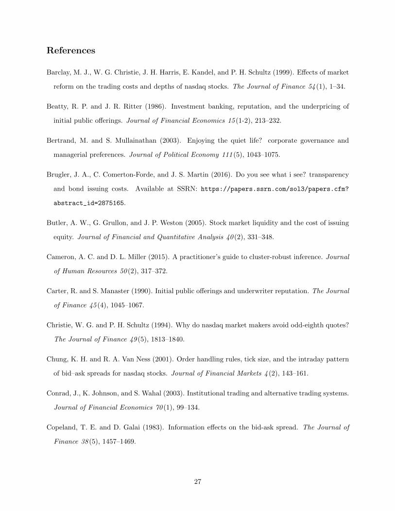
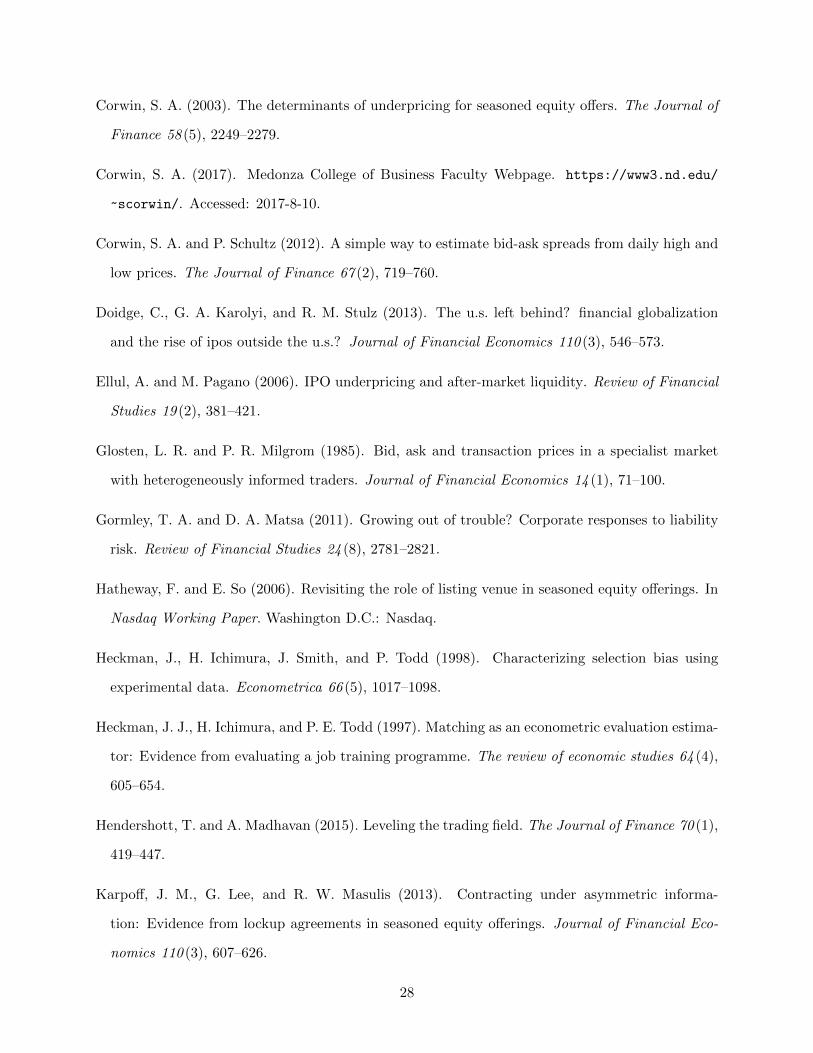
Table 1 contains summary statistics of our data. The mean SEO underpricing in our sample is

7We gratefully thank Jeffrey Smith for his assistance with providing this list.8While there is a very high degree of consistency across the two datasets, we use the Nasdaq trader alerts wherepossible as these are considered to be the most official record available according to Nasdaq economists.

9

2.98% with a standard deviation of 3.21%. The median underpricing is 2.03%, the average SEO

represents 27.1% of the current market capitalization of the firm, the average bid-ask spread is

2.30% and average one month standard deviation of returns is 3.00%. The equivalent Nasdaq

averages from Corwin (2003) are 2.72% for close to offer underpricing, 26.84% for relative size,

2.95% for bid-ask spread and 3.41% for one month standard deviation of returns. The data used

in Corwin (2003) covers 1980 to 1998 for the issuing characteristics and 1993 to 1998 for liquidity.

Table 1 about here

Table 2 contains correlation coefficients for our data. Underpricing is negatively correlated

with the value of the issue and market capitalization but positively correlated with relative size,

indicating that SEOs by larger companies tend to have less underpricing but that participants

in SEOs receive more compensation when companies raise relatively more capital. Volatility and

illiquidity (bid-ask and high-low spreads) are both positively correlated with underpricing while

the OHR dummy variable is negatively correlated with underpricing. The negative correlation

between the OHR dummy and underpricing at least partially reflects the fact that larger stocks

were phased in earlier in the program, as well as any potential causal relation running from liquidity

to underpricing.

Table 2 about here

Table 3 contains summary statistics over the period June 1996 to June 1998 split by exchange.

The second column of Table 3 contains the mean for Nasdaq issues, the third column contains

the means for all NYSE issues and the fourth column contains the t-statistic for a test of equal

means between Nasdaq and NYSE issues. The fifth column contains the means for a nearest-

neighbour matched sample of NYSE issues where matching is conducted on issue date, log of market

capitalization, log of stock price, volume traded, volatility and issue size using the inverted variance

weighting matrix (full details in Section 4.3). Table 3 indicates that SEOs on the Nasdaq tend to

be smaller but represent a larger fraction of existing equity capital and are more significantly

underpriced. The matching process reduces the gap between average Nasdaq and NYSE SEO

10

characteristics, but is unable to entirely eliminate the differences.9 There were also substantially

more SEOs taking place on the Nasdaq over our sample period than on the NYSE, as shown in

Figure 6.

Table 3 about here

4 Identification using the Order Handling Rules

Our approach to identifying the effect of liquidity on SEO underpricing exploits the change in

market structure following the introduction of the OHR as a shock to liquidity across Nasdaq

securities. The OHR reforms were designed to offer investors more competitive quotes via the

mandatory display by dealers of superior customer limit orders and the dissemination of superior

prices posted on proprietary trading venues such as ECNs. Subsequent studies by Barclay et al.

(1999), McInish et al. (1998) and Chung and Van Ness (2001) demonstrate that the OHR led to a

statistically and economically significant reduction in spreads (quoted and effective).

For our purposes, we use the OHR as a quasi-natural experiment that drives variation in

stock liquidity but that does not directly affect underpricing and is unrelated to potential omitted

variables such as information asymmetry. While the staggered introduction of the OHR was not

entirely random, (the first 13 waves were only drawn from the 1000 most actively traded issues),

there was a large degree of randomization within each wave. Indeed from August 4th onwards,

stocks were drawn randomly from the entire universe of Nasdaq issues (Smith, 1998). Furthermore,

selection into each wave was determined by relative trading activity (volume). Given the assignment

to waves on observables (trading volume) and the randomization within each wave combined with

the market-wide implementation of the new market structure, we argue that the OHR is appropriate

for our purposes.

4.1 Regression Specifications: Differences-in-Differences

We use the OHR dummy variable in three related econometric models. First, we use OHR status

as a treatment variable and estimate the effect of OHR status on SEO underpricing in a difference-

9We also use the Mahalanobis weighting matrix and the Euclidean weighting matrix but these generate worse matchesthan those using the inverted variance weights.

11

in-differences framework. The most general version of these regressions takes the form:

yit = γc + µt + βOHRit + ρ′xit + εit (1)

where yit is the underpricing of the ith SEO during time period t, OHRit is the OHR status of the

issue (1 if trading under the OHR at time of issue and 0 otherwise), xit is the vector of stock-specific

control variables defined in the period before the the start of OHR implementation, γc is a fixed

effect defined by membership of each of the phase-in waves (i.e. γj takes the value 1 if stock i

was included in the jth wave of stocks) and µt is a time fixed effect where time is defined either as

calendar month or by the series of dates at which new stocks were introduced to the OHR (i.e. ρj

takes the value 1 if the issue occurs in the jth month or between the OHR inclusion dates of the

jth and j + 1th waves, depending on how the time fixed effects are being defined).

With wave-cohort fixed effects and time fixed effects defined by the dates of each wave’s in-

troduction to the OHR, Equation (1) is analogous to a treatment effect around a single treatment

date, but where assignment to treatment or control occurs across multiple groups and periods. A

similar approach is used in both Bertrand and Mullainathan (2003) and Gormley and Matsa (2011)

and is also applied in the context of corporate bond issuing costs and transparency by Brugler,

Comerton-Forde, and Martin (2016). As discussed in Brugler et al. (2016), the parameter β is our

pooled analogue of the coefficient on the interacted term between the treatment dummy and the

post-treatment period dummy in a difference-in-difference model using a single treatment period.

It captures the average treatment effect across the multiple events. Pooling the 22 treatment dates

into a single regression allows us to control for cohort-specific effects and means we are not as re-

liant on the parallel trends assumption as we would be when analyzing the difference-in-difference

around a single event.

We estimate Equation (1) under four specifications: excluding controls and fixed effects (i.e.

regressing underpricing only on OHR status), including the controls, including controls and monthly

fixed effects, and including controls, wave-cohort fixed effects and time fixed effects based on wave

dates. As per Secton 3, the control variables in the relevant specifications are log of market

capitalization, relative size of SEO, volatility of mid-quote returns, log of stock price and log of

volume traded, defined in the period prior to the initial roll-out of the OHR where applicable.

12

Of course, implementation of the OHR is not truly random. If it were, arguably the most

rigorous way to estimate Equation (1) would be to exclude all control variables as inclusion of the

wave-cohort fixed effects can theoretically remove any time-invariant stock characteristics that may

affect SEO underpricing and differ systematically across cohorts. The fact that OHR status is driven

in part by relative trading volume motivates us to incorporate the controls, however estimating the

model without controls and only wave-cohort dummies does not affect our conclusions.10

We also estimate Equation (1) for three sub-samples of our data. The first two sub-samples

are based on market capitalization: we estimate Equation (1) for SEOs by companies with market

capitalizations below the sample median and for SEOs by companies with market capitalizations

above the sample median. These regressions are designed to allow for heterogeneous treatment

effects for OHR status between smaller and larger stocks. The third sub-sample includes all SEOs

that take place after June 2nd, 1997. These regressions are provided to address potential concerns

about the implementation of two additional trading rule changes that affect all Nasdaq stocks in

1997: the change in tick size from 1/8th to 1/16th on June 2nd, 1997 and Regulation M that

impacted the actions that deal participants could undertake around new securities offerings and

was implemented on March 4th, 1997. Although date fixed effects should theoretically account for

the market-wide impact of these changes, we include the regressions on a sub-sample where trading

rules were unchanged as an additional robustness check.

4.2 Regression Specifications: Instrumental Variables

The second way in which we exploit the OHR is as an instrumental variable (IV) for liquidity in

two-stage least squares (2SLS) underpricing regressions. The target regression model we wish to

estimate is:

yit = µt + βLiqit + ρ′xit + εit (2)

where Liqit is the liquidity (bid-ask or high-low spread) of stock i undergoing an SEO at time t

where liquidity is the averaged across the month preceding the issue date. Other variables are

defined as per Equation (1). Due to omitted variable bias and selection on unobservables, Liqit is

potentially correlated with the error term εit. Our solution to this problem is to instrument for

10These results are available upon request.

13

Liqit using the OHR status of the stock being issued.

The relevance requirement for our instrument is that the implementation of the OHR is asso-

ciated with an economically and statistically significant improvement in liquidity, and specifically

a reduction in spreads. Consistent with the evidence presented in Barclay et al. (1999), McInish

et al. (1998) and Chung and Van Ness (2001) our first stage regression results show that this result

also holds in our sample.

The exogeneity condition requires that, conditional on relevant control variables, our instrument

only affects underpricing through the liquidity channel, and (1) does not directly drive underpricing

itself or (2) affect underpricing through any other channel that is not controlled for. Our structural

estimates of the parameters in (2) are only just-identified, so we cannot provide evidence via

overidentifying restrictions, such as with a Sargan or Hansen J-test. Instead we must rely on the

pseudo-random nature of the OHR implementation schedule combined with the fully observable

nature of assignment to waves (based on trading activity) to justify the validity of our instrument.

For all models and specifications, we calculate White heteroskedasticity-robust standard errors

and report tests based on these standard errors. We have also estimated all models with stan-

dard errors clustered at the time level. Cameron and Miller (2015) note that parameter covariance

matrices can be downward biased when there are few clusters and that this problem can be particu-

larly problematic when the number of observations by clusters varies. Given the highly unbalanced

nature of the clusters in our sample and the relatively few clusters (either 10 or 23 depending on

how the time fixed effects are defined), we rely on our simple White standard errors. However, our

conclusions are not sensitive to clustering by time.

4.3 Regression Specifications: Comparisons with SEOs on the New York Stock

Exchange

Under the two specifications outlined in Sections 4.1 and 4.2, we use differences in OHR status

across Nasdaq stocks to identify the effect of market structure on capital costs. Although the OHR

provides us with a source of variation in stock liquidity that does not directly affect underpricing,

the nature of the roll-out of the program implies that OHR status is not truly random. As an

alternative to including OHR status directly as a regressor or instrument in an econometric model,

14

we instead analyse how underpricing and liquidity changed before and after the implementation of

the OHR for SEOs taking place on the Nasdaq exchange relative to a group of SEOs for which no

major change in market structure takes place, namely those that occur on the NYSE.

We compare Nasdaq and NYSE SEOs in a number of ways. First, we do a simple comparison of

means for underpricing and liquidity (bid-ask spreads and high-low spreads) between Nasdaq and

NYSE SEOs before the beginning of the implementation of the OHR. We then compare the means

for underpricing and liquidity between Nasdaq and NYSE SEOs after the implementation of the

OHR is complete and calculate the difference-in-differences in means. This difference-in-difference

provides a simple estimate of the degree to which SEO underpricing improved or deteriorated on

the venue where the OHR was implemented relative to a control venue with no change in market

structure. It also is identical to the treatment effect coefficient for a regression of underpricing or

liquidity on exchange dummies, time dummies for whether the SEO occurred before or after the

OHR implementation and an interaction term between exchange and time dummies:

yi = δ0 + δ1ti + δ2Nasi + τ tiNasi + εi (3)

where yi is the underpricing or liquidity of the ith SEO, ti is a dummy variable indicating whether

the ith SEO occurred after the OHR implementation, Nasi is a dummy variable for SEOs on the

Nasdaq.

An alternative way to calculate this difference-in-differences is to compare the change in mean

underpricing and liquidity for Nasdaq SEOs before and after the OHR implementation and compare

this to the change in NYSE SEOs over the same period. The difference-in-differences from doing

so is the same as calculating the differences-in-differences between Nasdaq and NYSE SEOs within

a given period, however this alternative representation allows us to isolate whether SEOs on the

Nasdaq or the NYSE are responsible for the results.

Interpreting the simple comparison of means between Nasdaq and NYSE SEOs is complicated by

systematic differences in characteristics of stocks listed on the two exchanges. Table 3 demonstrates

that companies undertaking SEOs on the NYSE in our sample period are larger and issue larger

amounts of stock. They also have higher prices and volume, better liquidity and lower volatility

than SEOs on the Nasdaq. Since we are comparing changes in means, these differences in average

15

characteristics do not necessarily invalidate our approach, however if trends in SEO underpricing

differ across stocks with different characteristics, then inference from this approach will be biased.

To deal with this, we again estimate a treatment effect model where treatment status is defined

by exchange status, with Nasdaq stocks as the “treated” group but we now include the control

variables capturing differences in SEO and stock characteristics. The estimated model is given by:

yi = δ0 + δ1ti + δ2Nasi + τ tiNasi + β′Xi + εi (4)

where yi, ti and Nasi are defined as in Equation (3) and Xi is the set of control variables. These

are issue date, SEO relative size, log of market capitalization, log of stock price, volume traded in

month prior to SEO and volatility of mid-quote returns in month prior to the SEO.

Next, we compare the difference in average underpricing or liquidity between Nasdaq SEOs and

a matched sample of NYSE SEOs both prior to the implementation of the OHR and following the

implementation of the OHR. Each Nasdaq SEO is matched to its nearest neighbour NYSE SEO

from the same period (pre- or post- OHR) where matching is conducted on the same SEO and stock

characteristics as used in the estimation of Equation (4). From these differences across Nasdaq and

matched NYSE SEOs within periods, we construct a matched difference-in-differences estimator in

the spirit of of Heckman, Ichimura, and Todd (1997), Heckman, Ichimura, Smith, and Todd (1998)

and Todd (2010). As per Todd (2010), this estimator for repeated cross-sections takes the form

α1 =1

NNasPost

{Y NasPost,i −

∑j∈INYSE

Post

W (i, j)Y NY SEPost,j

}− 1

NNasPre

{Y NasPre,i −

∑j∈INYSE

Pre

W (i, j)Y NY SEPre,j

}(5)

where Y et,i is the outcome variable (underpricing or liquidity) for the ith SEO, occurring in period

t ∈ {Pre, Post} on exchange e ∈ {Nasdaq,NY SE}, NNastime is the number of SEOs occurring on

the Nasdaq in period t, INYSEt is the set of indices of SEOs that occur on the NYSE in period

t ∈ {Pre, Post} and W (i, j) is a weighting function that takes the value 1 if the jth NYSE SEO is

the nearest neighbour match for the ith Nasdaq SEO and zero otherwise.

In the treatment effect literature, estimators of the form (5) are used to estimate a treatment

effect when systematic differences between participant and non-participant outcomes persist, even

after conditioning, which may be due to selection on unobservables, for example (i.e. violations of

16

the “strong ignorability” condition of Rosenbaum and Rubin (1983)). In our approach, taking the

difference-in-differences of the two matched estimators (i.e. before and after the OHR implemen-

tation) allows us to infer whether or not the effect of listing location on underpricing and liquidity

changed significantly after the introduction of the OHR on the Nasdaq exchange, while accounting

for differences in average characteristics which may change over time or imply different trends in

outcome variables.

We use the inverted variance weighting matrix to calculate each nearest neighbour as this

generated a better fit than either the Mahalanobis or Euclidean weights. We obtain very similar

results using these different weighting matrices but as the match quality is worse, we rely on the

inverted variance weights.

We lastly complement the estimation of (5) by estimating an additional matched difference-in-

differences estimator where we first match Nasdaq (NYSE) SEOs that occur after the implementa-

tion of the OHR with Nasdaq (NYSE) SEOs that occur prior to the implementation of the OHR.

We then calculate the difference in these two estimators. This estimator takes the form

α2 =1

NNasPost

{Y NasPost,i −

∑j∈INas

Post

W (i, j)Y NasPre,j

}− 1

NNY SEPost

{Y NY SEPost,i −

∑j∈INYSE

Post

W (i, j)Y NY SEPre,j

}(6)

where all variables are defined as in Equation (5). Equation (6) is analogous to our comparison of

the change in raw means from before and after the implementation of the OHR for Nasdaq SEOs

and NYSE SEOs respectively, while accounting for potential changes in the average characteristics

of SEOs across time.

Standard errors for the difference in raw means are calculated without assuming identical vari-

ances between sub-samples. We use a non-parametric bootstrap for calculating standard errors

in matched differences and White heteroskedasticity-robust standard errors for treatment effect

regressions (Equations (3) and (4)). We include all SEOs that take place between June 1996 and

Dec 1996 as our pre-OHR sample and those that take place between January 1998 and June 1998

as our post-OHR sample.

17

5 SEO Results

5.1 Difference-in-Differences Regressions

We begin our analysis with a discussion of our differences-in-differences estimates that treat the

Order Handling Rules as a quasi-random treatment effect and estimate its direct effect on under-

pricing. The parameter estimates and associated t-statistics for our pooled difference-in-differences

estimates of Equation (1) are contained in Table 4. Model A contains estimates from a regression

of SEO underpricing onto the OHR dummy and a constant term, without controls or fixed effects.

Model B contains analogous estimates but with the inclusion of the control variables described in

Section 4.1. Model C adds 10 calendar month time fixed effects to Model B. Model D includes

23 time fixed effects based on the roll-out dates of the OHR program and also cohort fixed ef-

fects for stocks in each wave of the OHR implementation schedule as well as the controls. Since

this specification most closely adheres to a standard difference-in-difference framework, it is our

preferred specification. Panel A of Table 4 contains results for all SEOs in our sample. Panel B

contains results for stocks with above and below median market capitalizations respectively. Panel

C contains results for regressions using only SEOs occuring after June 2nd, 1997.

Table 4 about here

For each of the models in Table 4, the OHR parameter is negative and significant at the 5% level

or better, indicating that SEOs for companies with stock trading under the OHR were underpriced

significantly less than SEOs of companies with stock yet to be phased into the program. In terms

of economic significance, underpricing is predicted to be between 1.4% to 2.2% lower for stocks

trading under the OHR compared with not for the full sample of SEOs, which represents between

47% to 68% of the sample standard deviation of underpricing. The magnitude of the parameter is

largest for our most general specification in Model D. Firm size and price are negatively related to

SEO underpricing and are significant at the 5% and 10% level depending on the specification. Offer

size, volatility and volume are all positively related to SEO underpricing, but none are significant

at the 10% level in any specification.

The key take-away from Panel A of Table 4 is that, using a model with granular cohort and

18

time fixed effects and control variables that are known to be related to OHR status, we estimate

that the Order Handling Rules led to a statistically and economically significant improvement in

SEO underpricing and therefore a reduction in one source of direct capital costs for firms. Under

this model, we can have a relatively high degree of confidence that conditional unconfoundedness

holds. Furthermore, since the Order Handling Rules are applied to none of the SEOs at the start

of our sample but apply to all SEOs by the end of it, with a significant period of overlap in the

second half of 1997, there is little concern about weak overlap between the “treated” and “control”

sub-populations in our data.

Panel B of Table 4 indicates that that the magnitude of the effect of the OHR was larger for

smaller stocks. For these stocks, the OHR led to a reduction in underpricing of between 1.6% and

3.5%. For larger stocks, the estimated effect of the OHR is between 0.9% and 1.4% depending on

the specification. However, SEOs by companies with smaller market capitalizations tend to be more

heavily underpriced than SEOs by larger companies. Comparing the size of the OHR parameters

across small and large stocks to the mean underpricing by sub-sample shows that the standardized

size of the effect is comparable across small and large stocks. For small stocks, the size of the effect

is between 40% and and 80% of the sub-sample mean of underpricing (4.36%). For large stocks,

the OHR coefficient represents betwen 55% and 80% of the sub-sample mean (1.7%). Nevertheless,

it is plausible that it is the absolute change in the cost of issuing equity capital that matters for

companies, not the relative change. If this is the case, then the results in Table 4 suggest that the

OHR was relatively more beneficial for smaller companies than larger companies.

The regressions in Panels A and B of Table 4 are estimated using data that spans the entire

roll-out of the OHR. During this period, two additional rule changes affected the trading of Nasdaq

stocks: the change in quotation tick size from one eighth to one sixteenth on June 2, 1997 and

Regulation M that was effectively implemented on March 4, 1997. Panel C of Table 4 show that the

OHR treatment effect is larger in the shorter sample, demonstrating that the possible confounding

effects earlier in 1997 are not responsible for the OHR treatment effect.

19

5.2 Instrumental Variable Regressions

As per Barclay et al. (1999), the OHR were specifically designed to offer investors more competitive

quotes and the rules were effective in achieving these ends. Clearly, one obvious channel by which the

OHR would drive changes in SEO underpricing is directly through liquidity. While it is not obvious

to us what other channels may be directly affected by the OHR, instrumental variable regressions

can help provide evidence that 1) the OHR did affect liquidity for the stocks in our sample and

2) the change in liquidity caused by the OHR was itself a key driver of the improvement in SEO

underpricing.

Parameter estimates and associated t-statistics for our IV regressions where liquidity is treated

as an endogenous regressor and the OHR dummy as the IV are contained in Tables 5 and 6.

In Table 5, the liquidity variable is the bid-ask spread while in Table 6, the liquidity variable

is the Corwin and Schultz (2012) high-low spread estimator. In both tables, Model A includes

only a constant term and the endogenous liquidity regressor that is instrumented for using the

OHR dummy. Model B adds control variables while Model C adds controls and calendar month

time fixed effects. Underneath the main regression estimates, we also report the first stage OHR

dummy coefficient and t-statistic, the Kleibergen-Paap LM test for full rank of the first stage Z ′X

matrix (underidentification), the Cragg-Donald Wald - F statistic for weak identification and the

F -statistic for the relevance of the instrument in the first stage regression. Note that since there

is a single instrument, the first stage F -statistic is simply the square of the t-statistic on the first

stage OHR coefficient.

Table 5 about here

In all three specifications in Table 5, the second stage coefficient on the bid-ask spread is

positive and both economically and statistically significant at the 5% level. The parameter is

between approximately 50% and 300% larger than the equivalent OLS regressions, which possibly

suggests that the OLS liquidity parameter estimates are biased towards zero.11 This may explain

to some degree the findings of Corwin (2003) that bid-ask spreads are only very weakly related to

SEO underpricing. Our second stage estimates suggest that an exogenous one standard deviation

11OLS regression results are available from the authors on request.

20

increase in bid-ask spreads would reduce SEO underpricing by between approximately 1.60% to

1.90%, or between about 50% to 60% of the sample standard deviation in underpricing. In all

three specifications, we reject the null of underidentification and weak identification, and first stage

F -statistics all exceed 10.

An alternative way to assess the magnitude of our second stage regressions is to calculate the

difference in expected underpricing for a stock with OHR status equal to one and one with OHR

status equal to zero. To do this, we simply multiply the first stage coefficient with the second stage

coefficient. Doing this yields expected changes in underpricing of between -1.40% to -1.55%. The

magnitude of these effects are very similar to that of the OHR dummy variable in the equivalent

difference-in-differences specifications in Table 4 and discussed in Section 5.1 (i.e. Models A, B

and C in Table 4). One interpretation of the high degree of similarity between our IV results and

our difference-in-differences results is that the causal effect of the OHR on SEO underpricing can

be almost fully explained by the degree to which the OHR improved liquidity. We interpret the

consistency in the magnitudes of effects across Tables 4 and 5 as supportive of the notion that OHR

affected underpricing primarily through the liquidity channel.

Table 6 about here

Turning to our IV regressions that use the high-low spread estimator of Corwin and Schultz

(2012), we find very similar results to those using the bid-ask spread. The second stage coefficients

on our illiquidity variable are all economically and statistically significant at the 5% level or better.

An exogenous one standard deviation increase high-low spreads would lead to a reduction in SEO

underpricing of between 2.15% and 2.25%, or approximately two thirds of one standard deviation

of underpricing in our sample. Calculating the magnitude of the effect for a stock trading in the

OHR compared with one that is not included in the OHR, we again predict an effect that is very

similar in size to those found in Models A, B and C of Table 4. We note that although the first

stage diagnostic tests reject the nulls of underidentification and weak identification for Models A

and B, for Model C we have some evidence of weak identification with a first stage F -statistic below

10 and the Cragg-Donald Wald test statistic below the relevant 10% Stock-Yogo critical values.

In both Tables 5 and 6, the other control variables have very similar interpretations as the

21

difference-in-differences specifications. Firm size and stock price are negatively related to SEO un-

derpricing, but this relationship is only statistically significant for stock price. Offer size, volatility

and trading volume are positively related to SEO underpricing. For the IV regressions using bid-ask

spreads, only trading volume is statistically significant at the 10% level or better (t-statistics of

2.32 and 1.93 in Models B and C respectively). For the regressions using the high-low estimator,

offer size is statistically significant at the 10% level when time fixed effects are included but the

volatility and volume are not significant under any specification.

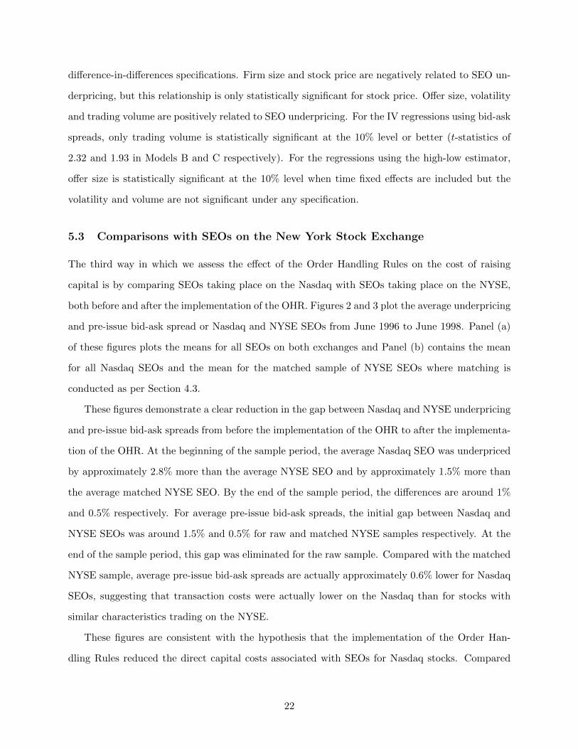
5.3 Comparisons with SEOs on the New York Stock Exchange

The third way in which we assess the effect of the Order Handling Rules on the cost of raising

capital is by comparing SEOs taking place on the Nasdaq with SEOs taking place on the NYSE,

both before and after the implementation of the OHR. Figures 2 and 3 plot the average underpricing

and pre-issue bid-ask spread or Nasdaq and NYSE SEOs from June 1996 to June 1998. Panel (a)

of these figures plots the means for all SEOs on both exchanges and Panel (b) contains the mean

for all Nasdaq SEOs and the mean for the matched sample of NYSE SEOs where matching is

conducted as per Section 4.3.

These figures demonstrate a clear reduction in the gap between Nasdaq and NYSE underpricing

and pre-issue bid-ask spreads from before the implementation of the OHR to after the implementa-

tion of the OHR. At the beginning of the sample period, the average Nasdaq SEO was underpriced

by approximately 2.8% more than the average NYSE SEO and by approximately 1.5% more than

the average matched NYSE SEO. By the end of the sample period, the differences are around 1%

and 0.5% respectively. For average pre-issue bid-ask spreads, the initial gap between Nasdaq and

NYSE SEOs was around 1.5% and 0.5% for raw and matched NYSE samples respectively. At the

end of the sample period, this gap was eliminated for the raw sample. Compared with the matched

NYSE sample, average pre-issue bid-ask spreads are actually approximately 0.6% lower for Nasdaq

SEOs, suggesting that transaction costs were actually lower on the Nasdaq than for stocks with

similar characteristics trading on the NYSE.

These figures are consistent with the hypothesis that the implementation of the Order Han-

dling Rules reduced the direct capital costs associated with SEOs for Nasdaq stocks. Compared

22

with a sample of SEOs for which no major change in market structure took place (NYSE issues),

underpricing and bid-ask spreads fell after the OHR. To assess the statistical significance of these

results, we estimate the difference-in-difference in average Nasdaq and NYSE SEO underpricing

and liquidity from before to after the OHR rollout and formally test whether the gap between

Nasdaq and NYSE SEOs fell after the OHR. Table 7 contains difference-in-differences in means for

underpricing and pre-issue liquidity for SEOs on the two exchanges in the June 1996 to December

1996, pre-OHR period and the January 1998 to December 1998, post-OHR period, as per Section

4.3.

Panel A of Table 7 compares the simple difference in means. The first row of Panel A contains

the difference in means for SEO underpricing, bid-ask spreads and high-low spreads between Nasdaq

and NYSE SEOs in the pre-OHR period with t-statistics in parenthesis. The second row of Panel A

contains the same difference in means across exchanges in the post-OHR period. These results show

a significant decline in the average difference in SEO underpricing between Nasdaq and NYSE stocks

after the implementation of the OHR (Column 1). In the pre-OHR period, the average underpricing

of a Nasdaq issues is 2.79% larger than for NYSE issues. After the implementation of the OHR,

the average underpricing of Nasdaq issues is only 1.04% more than for NYSE issues, a reduction

of 1.75% in the difference between the two exchanges (contained in the fifth row of Panel A). This

difference-in-differences represents approximately 55% of the standard deviation of Nasdaq SEO

underpricing and is statistically significant at the 1% level. The same rows for columns 2 and

3 demonstrate a reduction in average pre-issue bid-ask spreads of 1.1% and high-low spreads of

0.58%.

The third and fourth rows of Panel A contain the change in mean underpricing within each

exchange from before and after OHR implementation. While the difference-in-differences between

rows three and four of Panel A are (by construction) identical to the difference-in-differences be-

tween rows two and three, we include these additional results to demonstrate that the reduction in

the gap between Nasdaq and NYSE SEOs is concentrated in Nasdaq SEOs. As expected for the

NYSE, there is no significant change in underpricing or liquidity from before to after OHR imple-

mentation while on the Nasdaq we observe significant reductions in underpricing, bid-ask spreads

and high-low spreads.

As discussed in Section 4.3 and clearly demonstrated in Table 3, there are systematic differences

23

in average SEO characteristics between the Nasdaq and the NYSE. Companies undertaking a

secondary offering on the NYSE tend to be larger, trade more frequently, with less volatility and

are more liquid than their counterparts on the Nasdaq. While this does not necessarily invalidate

the comparison of means, the possibility for differences in trends across SEOs of different companies

could potentially confound the interpretation of these results. If for example, there are different

trends in the underpricing or liquidity for SEOs by larger companies relative to smaller companies,

we would conflate the effect of the OHR with these different trends.

We address this issue in two ways. First, we estimate a simple treatment effect model which

includes a post-OHR dummy, a Nasdaq dummy, an interaction term for these dummies and SEO

and stock characteristics as control variables. The econometric model is given by Equation (4).

The treatment effect coefficient with controls is contained in the sixth row of Panel A. These

coefficients show that the difference-in-difference in underpricing and liquidity remain economically

and statistically significant after controlling for issue and stock characteristics. For liquidity, the

magnitude of the effects are almost identical to the simple difference-in-differences of unadjusted

means. For underpricing, the size of the effect is slightly diminished (1.39% compared with 1.75%)

but is still significant at the 1% level.

The second way we address the issue of systematic differences in issue and stock characteristics

across exchanges is by estimating the difference between average underpricing and liquidity for

Nasdaq SEOs and a matched sample of NYSE SEOs for both the pre- and post-OHR periods

using the matching process described in Section 4.3. We then construct the matched difference-in-

differences estimate across the two periods similar to Heckman et al. (1997) and Heckman et al.

(1998). The matched difference-in-differences estimates are contained in Panel B. The first row of

Panel B contains the difference in mean between Nasdaq SEO underpricing and liquidity and the

matched sample NYSE SEO for SEOs conducted prior to the OHR implementation. The second

row of Panel B contains the same difference in mean for the period after the implementation of the

OHR. The third column contains the difference-in-differences in means between the two periods.

Similar to the results using the full NYSE sample, the gap in underpricing between Nasdaq and

NYSE stocks is higher before the implementation of the OHR relative to after its implementation.

Prior to the OHR, Nasdaq SEOs were, on average, underpriced by 1.64% more than the matched

NYSE counterparts. After the OHR, the gap between Nasdaq and NYSE SEO underpricing fell

24

to 0.49%, a difference-in-differences of 1.16% with an associated bootstrapped t-statistic of -2.05.

While the magnitude of the reduction in the underpricing gap is less than that estimated using

unadjusted means or a treatment effects framework with issue and stock controls, it does represent

a reduction of approxmately one third of the sample standard deviation of underpricing for Nasdaq

SEOs.

In the fourth, fifth and sixth rows of Panel B, we first match each Nasdaq SEO in the post-

OHR period with its nearest neighbour Nasdaq SEO in the pre-OHR period and do the same for

NYSE SEOs. We then take the difference of these two matched differences to compare whether

Nasdaq SEO underpricing fell relative to NYSE SEO underpricing over the sample period. Like

rows three and four of Panel A, these help us to discern whether the net effect is due to changes in

the Nasdaq (as we would expect) or the NYSE. These estimates have an advantage over matching

within periods across exchanges as the latter suffers from the fact that there are approximately

twice as many Nasdaq SEO as there are NYSE SEOs in either period, which makes it difficult to

find good matches for Nasdaq SEOs in the NYSE sub-samples. By matching across periods within

exchanges, the control groups actually have more members than the treated group, which arguably

helps the power of our estimate.

Using our matched difference-in-differences after first matching across periods within each ex-

change, we again observe that underpricing and pre-issue liquidity both improved significantly for

SEOs on the Nasdaq without any statistically or economically significant change in NYSE issues.

For Nasdaq SEOs, average underpricing fell by 1.1% after OHR implementation relative to the

matched sample from the same exchange before the OHR is implemented. For the NYSE, the

change in underpricing is very close to zero and is not statistically significant at the 10% level or

better. The matched difference-in-differences is 1.2% and is significant at the 1% level. For pre-issue

liquidity, we also observe a significant improvement in Nasdaq stocks from before to after the OHR,

without any concurrent significant change in NYSE stocks. The matched difference-in-differences

are of similar magnitudes to those in Panel A and are statistically significant at the 1% level.

Taken together, Figures 2 and 3 and Table 7 demonstrate that SEO underpricing and liquidity

improved on the Nasdaq following the implementation of the Order Handling Rules without any

discernable effect on underpricing and liquidity for stocks issuing on the NYSE. Economically, the

relative reduction in underpricing ranges from 1.16% to 1.75% depending on the specification, while

25

reductions in bid-ask spreads and high-low spreads are between 1.00% and 1.1% and 0.52% and

0.58% respectively. All of our difference-in-differences estimates are statisically significant at the

5% level and for all but one estimate, they are significant at the 1% level.

6 Conclusion

In the 1990s Nasdaq transformed from a dealer-oriented over-the-counter market to a market where

investors could directly interact with each other. The reforms were phased in across stocks over

time allowing for identification of their impact on firms’ cost of raising capital. We find that the

reforms significantly reduced the underpricing of seasoned equity offerings by one to two percentage

points from a pre-OHR average of 3.6 percent. Using the staggered introduction of the OHR as an

instrument shows improved secondary market liquidity drives the reduction in underpricing.

Studying the impact of market structure and liquidity on the cost of raising capital is impor-

tant for policy and academic reasons. For academics it provides a deeper understanding of the

link between secondary-market liquidity, investment, and capital structure. The decline in the

number of IPOs and publicly listed firms in the U.S. (Doidge et al., 2013) has prompted legislation

requiring market structure experiments like the 2016 SEC tick-size pilot. Our results suggest that

market structure reforms reducing intermediation lower the costs of raising capital. To the extent

that the stock market suffers from excess intermediation and illiquidity, carefully crafted market

structure reforms could improve investment and risk sharing in the economy.12 The results also

have implications for other asset classes. For example, corporate bonds traditionally trade over-

the-counter. Market structure innovations increasing dealer competition, such as request-for-quote

auctions (Hendershott and Madhavan, 2015), and enabling direct transactions between investors

can lower the cost of debt issuance.

12A possible source of excess intermediation and illiquidity is high-frequency traders, but there is little academic researchsupport for this.

26

References

Barclay, M. J., W. G. Christie, J. H. Harris, E. Kandel, and P. H. Schultz (1999). Effects of market

reform on the trading costs and depths of nasdaq stocks. The Journal of Finance 54 (1), 1–34.

Beatty, R. P. and J. R. Ritter (1986). Investment banking, reputation, and the underpricing of

initial public offerings. Journal of Financial Economics 15 (1-2), 213–232.

Bertrand, M. and S. Mullainathan (2003). Enjoying the quiet life? corporate governance and

managerial preferences. Journal of Political Economy 111 (5), 1043–1075.

Brugler, J. A., C. Comerton-Forde, and J. S. Martin (2016). Do you see what i see? transparency

and bond issuing costs. Available at SSRN: https://papers.ssrn.com/sol3/papers.cfm?

abstract_id=2875165.

Butler, A. W., G. Grullon, and J. P. Weston (2005). Stock market liquidity and the cost of issuing

equity. Journal of Financial and Quantitative Analysis 40 (2), 331–348.

Cameron, A. C. and D. L. Miller (2015). A practitioner’s guide to cluster-robust inference. Journal

of Human Resources 50 (2), 317–372.

Carter, R. and S. Manaster (1990). Initial public offerings and underwriter reputation. The Journal

of Finance 45 (4), 1045–1067.

Christie, W. G. and P. H. Schultz (1994). Why do nasdaq market makers avoid odd-eighth quotes?

The Journal of Finance 49 (5), 1813–1840.

Chung, K. H. and R. A. Van Ness (2001). Order handling rules, tick size, and the intraday pattern

of bid–ask spreads for nasdaq stocks. Journal of Financial Markets 4 (2), 143–161.

Conrad, J., K. Johnson, and S. Wahal (2003). Institutional trading and alternative trading systems.

Journal of Financial Economics 70 (1), 99–134.

Copeland, T. E. and D. Galai (1983). Information effects on the bid-ask spread. The Journal of

Finance 38 (5), 1457–1469.

27

Corwin, S. A. (2003). The determinants of underpricing for seasoned equity offers. The Journal of

Finance 58 (5), 2249–2279.

Corwin, S. A. (2017). Medonza College of Business Faculty Webpage. https://www3.nd.edu/

~scorwin/. Accessed: 2017-8-10.

Corwin, S. A. and P. Schultz (2012). A simple way to estimate bid-ask spreads from daily high and

low prices. The Journal of Finance 67 (2), 719–760.

Doidge, C., G. A. Karolyi, and R. M. Stulz (2013). The u.s. left behind? financial globalization

and the rise of ipos outside the u.s.? Journal of Financial Economics 110 (3), 546–573.

Ellul, A. and M. Pagano (2006). IPO underpricing and after-market liquidity. Review of Financial

Studies 19 (2), 381–421.

Glosten, L. R. and P. R. Milgrom (1985). Bid, ask and transaction prices in a specialist market

with heterogeneously informed traders. Journal of Financial Economics 14 (1), 71–100.

Gormley, T. A. and D. A. Matsa (2011). Growing out of trouble? Corporate responses to liability

risk. Review of Financial Studies 24 (8), 2781–2821.

Hatheway, F. and E. So (2006). Revisiting the role of listing venue in seasoned equity offerings. In

Nasdaq Working Paper. Washington D.C.: Nasdaq.

Heckman, J., H. Ichimura, J. Smith, and P. Todd (1998). Characterizing selection bias using

experimental data. Econometrica 66 (5), 1017–1098.

Heckman, J. J., H. Ichimura, and P. E. Todd (1997). Matching as an econometric evaluation estima-

tor: Evidence from evaluating a job training programme. The review of economic studies 64 (4),

605–654.

Hendershott, T. and A. Madhavan (2015). Leveling the trading field. The Journal of Finance 70 (1),

419–447.

Karpoff, J. M., G. Lee, and R. W. Masulis (2013). Contracting under asymmetric informa-

tion: Evidence from lockup agreements in seasoned equity offerings. Journal of Financial Eco-

nomics 110 (3), 607–626.

28

Kyle, A. S. (1985). Continuous auctions and insider trading. Econometrica 38 (5), 1315–1335.

Lee, G. and R. W. Masulis (2009). Seasoned equity offerings: Quality of accounting information

and expected flotation costs. Journal of Financial Economics 92 (3), 443–469.

Madhavan, A. (2000). Market microstructure: A survey. The Journal of Financial Markets 3 (3),

205–258.

McInish, T. H., B. F. Van Ness, and R. A. Van Ness (1998). The effect of the sec’s order-handling

rules on nasdaq. Journal of Financial Research 21 (3), 247–254.

Nasdaq (2017). Equity Trader Alert Index, 1997. https://www.nasdaqtrader.com/Trader.aspx?

id=archiveheadlines&cat_id=2/. Accessed: 2017-8-1.

Rock, K. (1986). Why new issues are underpriced. Journal of Financial Economics 15 (1-2),

187–212.

Rosenbaum, P. R. and D. B. Rubin (1983). The central role of the propensity score in observational

studies for causal effects. Biometrika 70 (1), 41–55.

Safieddine, A. and W. J. Wilhelm (1996). An empirical investigation of short-selling activity prior

to seasoned equity offerings. The Journal of Finance 51 (2), 729–749.

Smith, J. W. (1998). The effects of order handling rules and 16ths on nasdaq: A cross-sectional

analysis. In NASD Working Paper 98–02. Washington D.C.: NASD Inc.

Todd, P. E. (2010). Matching estimators. In Microeconometrics, pp. 108–121. Springer.

Weston, J. P. (2000). Competition on the nasdaq and the impact of recent market reforms. The

Journal of Finance 55 (6), 2565–2598.

29

Tables and Figures

Table 1: Summary Statistics - Nasdaq SEOs

This table reports means, standard deviations, minimums, maximums and 25th, 50th and 75th quantiles for offering and tradingcharacteristics for our sample. The sample includes SEOs on the Nasdaq occurring between January 1, 1997 and October 31,1997 that meet the selection criteria outlined in Section 3. Underpricing is defined as the negative of the log return from theprevious closing price to the offer price in percentage terms. The value of the offer is the offer price times the number of sharesissued in $ millions. Relative size is the ratio of the offer value to the market capitalization. The market capitalization is thenumber of shares outstanding times the closing price as at January 2, 1997. Ln(Price) is the log of the closing price as atJanuary 2, 1997. Volume is the dollar volume traded in the month of December, 1996 in $ millions. Volatility is the standarddeviation of daily mid-quote returns during December, 1996. Bid-ask is the average of the log of the closing ask price dividedby the log of the closing bid price in CRSP in the 21 trading days before the issue date. Hi-Lo is the Corwin-Schultz high-lowspread estimate for the month preceding the issue date. OHR is a dummy variable taking the value 1 if the stock of the companymaking an SEO is trading under the Nasdaq Order Handling Rules and 0 otherwise. All variables excluding log of price andthe OHR dummy are Winsorized at the 1% level. There are 196 SEOs meeting our selection criteria.

Mean Std. Dev Min 25% 50% 75% Max

Panel A: All Observations

Underpricing 2.98 3.21 -2.09 0.74 2.03 4.10 20.2

Value ($m) 79.4 79.0 7.57 33.0 54.7 96.0 686

Relative Size 0.27 0.17 0.02 0.15 0.24 0.33 1.03

MarketCap ($m) 333 447 16.1 94.5 175 423 3316

Ln(MarketCap) 5.25 1.05 2.78 4.55 5.17 6.05 8.11

Ln(Price) 2.88 0.57 1.25 2.56 2.88 3.26 4.35

Volume ($m) 55.2 92.9 0.15 6.87 21.6 60.3 662

Volatility 3.00 1.45 0.32 2.09 2.75 3.98 8.43

BidAsk (%) 2.30 1.40 0.31 1.32 1.99 2.95 8.75

HiLo 1.47 0.81 0.33 0.89 1.33 1.79 5.47

OHR 0.39 0.49 0.00 0.00 0.00 1.00 1.00

Panel B: Observations by OHR Status

BidAsk (%) - OHR 1.49 0.78 0.31 0.86 1.45 1.90 4.43

BidAsk (%) - Non OHR 2.83 1.46 0.68 1.76 2.46 3.60 8.75

HiLo - OHR 1.11 0.42 0.40 0.80 1.07 1.38 2.18

HiLo - Non OHR 1.69 0.91 0.33 1.03 1.51 2.11 5.47

Underpricing - OHR 2.03 2.50 -0.49 0.39 1.36 2.67 11.7

Underpricing - Non-OHR 3.60 3.48 -2.09 1.08 2.67 5.81 20.2

30

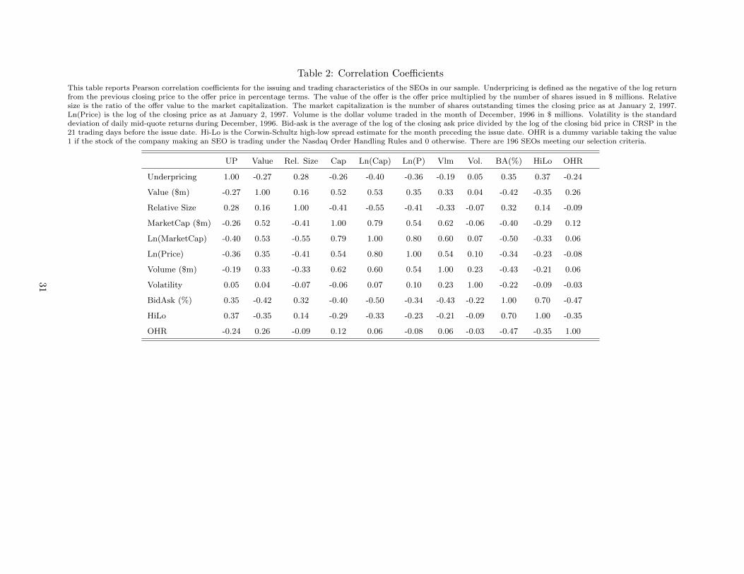
Table 2: Correlation Coefficients

This table reports Pearson correlation coefficients for the issuing and trading characteristics of the SEOs in our sample. Underpricing is defined as the negative of the log returnfrom the previous closing price to the offer price in percentage terms. The value of the offer is the offer price multiplied by the number of shares issued in $ millions. Relativesize is the ratio of the offer value to the market capitalization. The market capitalization is the number of shares outstanding times the closing price as at January 2, 1997.Ln(Price) is the log of the closing price as at January 2, 1997. Volume is the dollar volume traded in the month of December, 1996 in $ millions. Volatility is the standarddeviation of daily mid-quote returns during December, 1996. Bid-ask is the average of the log of the closing ask price divided by the log of the closing bid price in CRSP in the21 trading days before the issue date. Hi-Lo is the Corwin-Schultz high-low spread estimate for the month preceding the issue date. OHR is a dummy variable taking the value1 if the stock of the company making an SEO is trading under the Nasdaq Order Handling Rules and 0 otherwise. There are 196 SEOs meeting our selection criteria.

UP Value Rel. Size Cap Ln(Cap) Ln(P) Vlm Vol. BA(%) HiLo OHR

Underpricing 1.00 -0.27 0.28 -0.26 -0.40 -0.36 -0.19 0.05 0.35 0.37 -0.24

Value ($m) -0.27 1.00 0.16 0.52 0.53 0.35 0.33 0.04 -0.42 -0.35 0.26

Relative Size 0.28 0.16 1.00 -0.41 -0.55 -0.41 -0.33 -0.07 0.32 0.14 -0.09

MarketCap ($m) -0.26 0.52 -0.41 1.00 0.79 0.54 0.62 -0.06 -0.40 -0.29 0.12

Ln(MarketCap) -0.40 0.53 -0.55 0.79 1.00 0.80 0.60 0.07 -0.50 -0.33 0.06

Ln(Price) -0.36 0.35 -0.41 0.54 0.80 1.00 0.54 0.10 -0.34 -0.23 -0.08

Volume ($m) -0.19 0.33 -0.33 0.62 0.60 0.54 1.00 0.23 -0.43 -0.21 0.06

Volatility 0.05 0.04 -0.07 -0.06 0.07 0.10 0.23 1.00 -0.22 -0.09 -0.03

BidAsk (%) 0.35 -0.42 0.32 -0.40 -0.50 -0.34 -0.43 -0.22 1.00 0.70 -0.47

HiLo 0.37 -0.35 0.14 -0.29 -0.33 -0.23 -0.21 -0.09 0.70 1.00 -0.35

OHR -0.24 0.26 -0.09 0.12 0.06 -0.08 0.06 -0.03 -0.47 -0.35 1.00

31

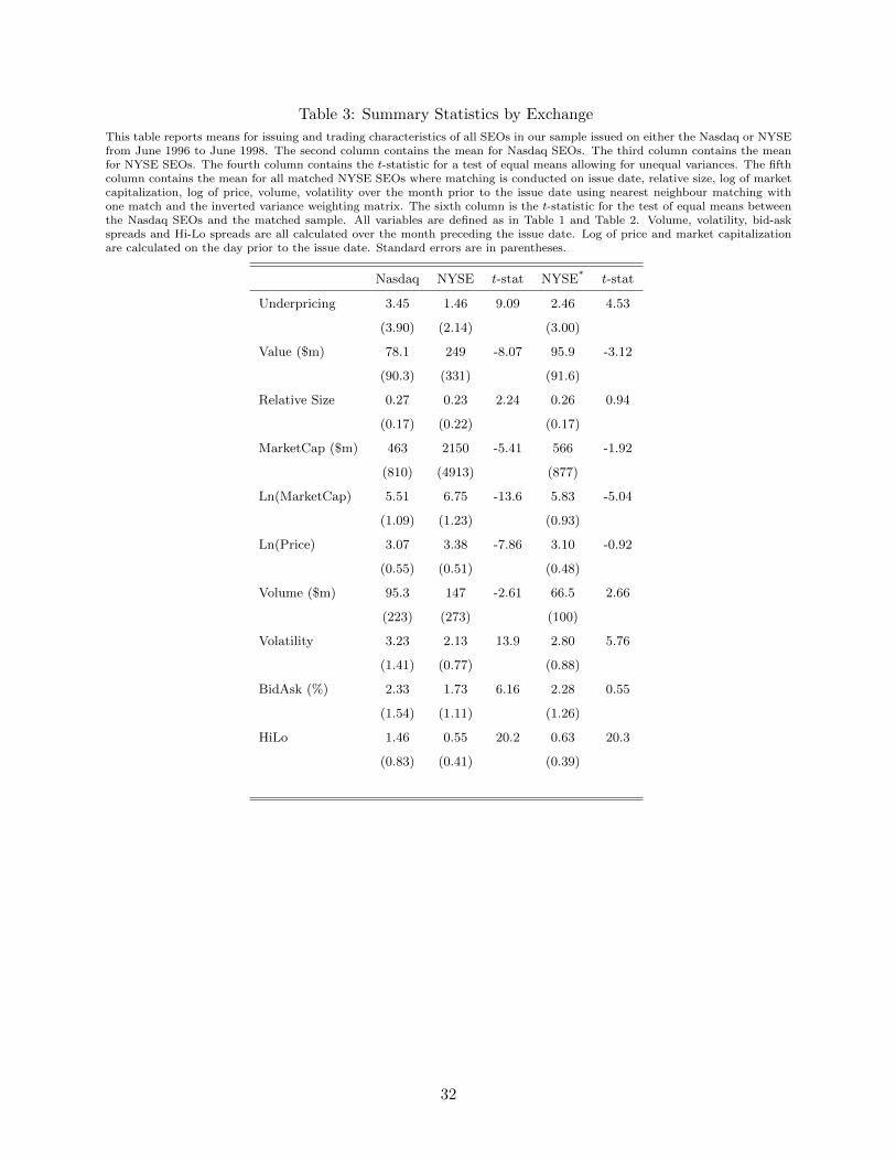
Table 3: Summary Statistics by Exchange

This table reports means for issuing and trading characteristics of all SEOs in our sample issued on either the Nasdaq or NYSEfrom June 1996 to June 1998. The second column contains the mean for Nasdaq SEOs. The third column contains the meanfor NYSE SEOs. The fourth column contains the t-statistic for a test of equal means allowing for unequal variances. The fifthcolumn contains the mean for all matched NYSE SEOs where matching is conducted on issue date, relative size, log of marketcapitalization, log of price, volume, volatility over the month prior to the issue date using nearest neighbour matching withone match and the inverted variance weighting matrix. The sixth column is the t-statistic for the test of equal means betweenthe Nasdaq SEOs and the matched sample. All variables are defined as in Table 1 and Table 2. Volume, volatility, bid-askspreads and Hi-Lo spreads are all calculated over the month preceding the issue date. Log of price and market capitalizationare calculated on the day prior to the issue date. Standard errors are in parentheses.

Nasdaq NYSE t-stat NYSE* t-stat

Underpricing 3.45 1.46 9.09 2.46 4.53

(3.90) (2.14) (3.00)

Value ($m) 78.1 249 -8.07 95.9 -3.12

(90.3) (331) (91.6)

Relative Size 0.27 0.23 2.24 0.26 0.94

(0.17) (0.22) (0.17)

MarketCap ($m) 463 2150 -5.41 566 -1.92

(810) (4913) (877)

Ln(MarketCap) 5.51 6.75 -13.6 5.83 -5.04

(1.09) (1.23) (0.93)

Ln(Price) 3.07 3.38 -7.86 3.10 -0.92

(0.55) (0.51) (0.48)

Volume ($m) 95.3 147 -2.61 66.5 2.66

(223) (273) (100)

Volatility 3.23 2.13 13.9 2.80 5.76

(1.41) (0.77) (0.88)

BidAsk (%) 2.33 1.73 6.16 2.28 0.55

(1.54) (1.11) (1.26)

HiLo 1.46 0.55 20.2 0.63 20.3

(0.83) (0.41) (0.39)

32

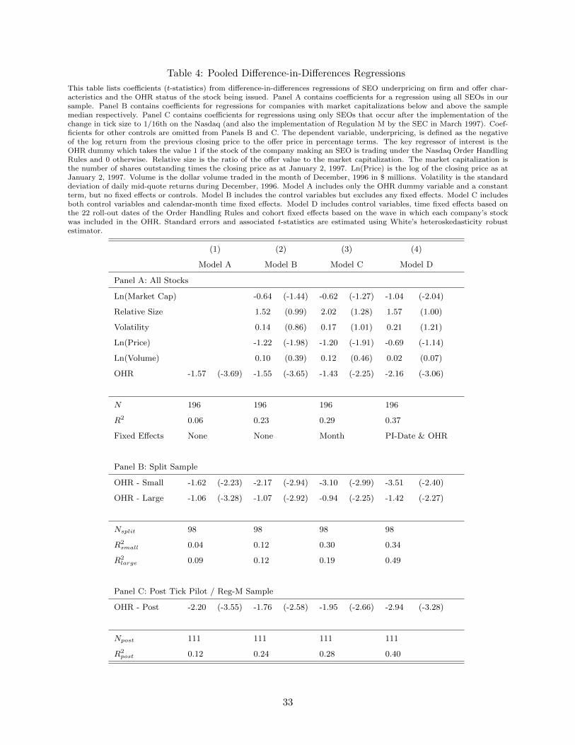
Table 4: Pooled Difference-in-Differences Regressions

This table lists coefficients (t-statistics) from difference-in-differences regressions of SEO underpricing on firm and offer char-acteristics and the OHR status of the stock being issued. Panel A contains coefficients for a regression using all SEOs in oursample. Panel B contains coefficients for regressions for companies with market capitalizations below and above the samplemedian respectively. Panel C contains coefficients for regressions using only SEOs that occur after the implementation of thechange in tick size to 1/16th on the Nasdaq (and also the implementation of Regulation M by the SEC in March 1997). Coef-ficients for other controls are omitted from Panels B and C. The dependent variable, underpricing, is defined as the negativeof the log return from the previous closing price to the offer price in percentage terms. The key regressor of interest is theOHR dummy which takes the value 1 if the stock of the company making an SEO is trading under the Nasdaq Order HandlingRules and 0 otherwise. Relative size is the ratio of the offer value to the market capitalization. The market capitalization isthe number of shares outstanding times the closing price as at January 2, 1997. Ln(Price) is the log of the closing price as atJanuary 2, 1997. Volume is the dollar volume traded in the month of December, 1996 in $ millions. Volatility is the standarddeviation of daily mid-quote returns during December, 1996. Model A includes only the OHR dummy variable and a constantterm, but no fixed effects or controls. Model B includes the control variables but excludes any fixed effects. Model C includesboth control variables and calendar-month time fixed effects. Model D includes control variables, time fixed effects based onthe 22 roll-out dates of the Order Handling Rules and cohort fixed effects based on the wave in which each company’s stockwas included in the OHR. Standard errors and associated t-statistics are estimated using White’s heteroskedasticity robustestimator.

(1) (2) (3) (4)

Model A Model B Model C Model D

Panel A: All Stocks

Ln(Market Cap) -0.64 (-1.44) -0.62 (-1.27) -1.04 (-2.04)

Relative Size 1.52 (0.99) 2.02 (1.28) 1.57 (1.00)

Volatility 0.14 (0.86) 0.17 (1.01) 0.21 (1.21)

Ln(Price) -1.22 (-1.98) -1.20 (-1.91) -0.69 (-1.14)

Ln(Volume) 0.10 (0.39) 0.12 (0.46) 0.02 (0.07)

OHR -1.57 (-3.69) -1.55 (-3.65) -1.43 (-2.25) -2.16 (-3.06)

N 196 196 196 196

R2 0.06 0.23 0.29 0.37

Fixed Effects None None Month PI-Date & OHR

Panel B: Split Sample

OHR - Small -1.62 (-2.23) -2.17 (-2.94) -3.10 (-2.99) -3.51 (-2.40)

OHR - Large -1.06 (-3.28) -1.07 (-2.92) -0.94 (-2.25) -1.42 (-2.27)

Nsplit 98 98 98 98

R2small 0.04 0.12 0.30 0.34

R2large 0.09 0.12 0.19 0.49

Panel C: Post Tick Pilot / Reg-M Sample

OHR - Post -2.20 (-3.55) -1.76 (-2.58) -1.95 (-2.66) -2.94 (-3.28)

Npost 111 111 111 111

R2post 0.12 0.24 0.28 0.40

33

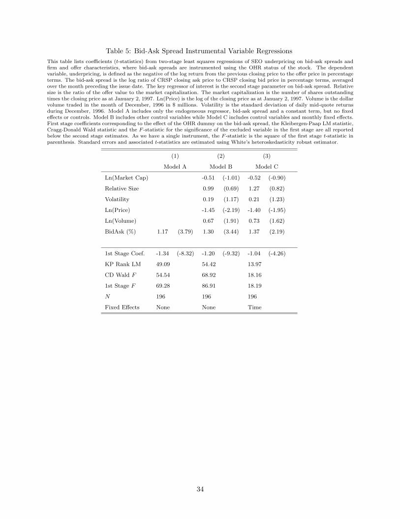
Table 5: Bid-Ask Spread Instrumental Variable Regressions

This table lists coefficients (t-statistics) from two-stage least squares regressions of SEO underpricing on bid-ask spreads andfirm and offer characteristics, where bid-ask spreads are instrumented using the OHR status of the stock. The dependentvariable, underpricing, is defined as the negative of the log return from the previous closing price to the offer price in percentageterms. The bid-ask spread is the log ratio of CRSP closing ask price to CRSP closing bid price in percentage terms, averagedover the month preceding the issue date. The key regressor of interest is the second stage parameter on bid-ask spread. Relativesize is the ratio of the offer value to the market capitalization. The market capitalization is the number of shares outstandingtimes the closing price as at January 2, 1997. Ln(Price) is the log of the closing price as at January 2, 1997. Volume is the dollarvolume traded in the month of December, 1996 in $ millions. Volatility is the standard deviation of daily mid-quote returnsduring December, 1996. Model A includes only the endogeneous regressor, bid-ask spread and a constant term, but no fixedeffects or controls. Model B includes other control variables while Model C includes control variables and monthly fixed effects.First stage coefficients corresponding to the effect of the OHR dummy on the bid-ask spread, the Kleibergen-Paap LM statistic,Cragg-Donald Wald statistic and the F -statistic for the significance of the excluded variable in the first stage are all reportedbelow the second stage estimates. As we have a single instrument, the F -statistic is the square of the first stage t-statistic inparenthesis. Standard errors and associated t-statistics are estimated using White’s heteroskedasticity robust estimator.

(1) (2) (3)

Model A Model B Model C

Ln(Market Cap) -0.51 (-1.01) -0.52 (-0.90)

Relative Size 0.99 (0.69) 1.27 (0.82)

Volatility 0.19 (1.17) 0.21 (1.23)

Ln(Price) -1.45 (-2.19) -1.40 (-1.95)

Ln(Volume) 0.67 (1.91) 0.73 (1.62)

BidAsk (%) 1.17 (3.79) 1.30 (3.44) 1.37 (2.19)

1st Stage Coef. -1.34 (-8.32) -1.20 (-9.32) -1.04 (-4.26)

KP Rank LM 49.09 54.42 13.97

CD Wald F 54.54 68.92 18.16

1st Stage F 69.28 86.91 18.19

N 196 196 196

Fixed Effects None None Time

34

Table 6: High-Low Spread Instrumental Variable Regressions

This table lists coefficients (t-statistics) from two-stage least squares regressions of SEO underpricing on Corwin and Schultz(2012) high-low spread estimates and firm and offer characteristics, where high-low spreads are instrumented using the OHRstatus of the stock. The dependent variable, underpricing, is defined as the negative of the log return from the previous closingprice to the offer price in percentage terms. The high-low spread is the monthly spread estimate provided by Corwin (2017).The key regressor of interest is the second stage parameter on high-low spread. Relative size is the ratio of the offer value tothe market capitalization. The market capitalization is the number of shares outstanding times the closing price as at January2, 1997. Ln(Price) is the log of the closing price as at January 2, 1997. Volume is the dollar volume traded in the month ofDecember, 1996 in $ millions. Volatility is the standard deviation of daily mid-quote returns during December, 1996. ModelA includes only the endogeneous regressor, high-low spread, and a constant term, but no fixed effects or controls. Model Bincludes other control variables while Model C includes control variables and monthly fixed effects. First stage coefficientscorresponding to the effect of the OHR dummy on the high-low spread, the Kleibergen-Paap LM statistic, Cragg-Donald Waldstatistic and the F -statistic for the significance of the excluded variable in the first stage are all reported below the second stageestimates. As we have a single instrument, the F -statistic is the square of the first stage t-statistic in parenthesis. Standarderrors and associated t-statistics are estimated using White’s heteroskedasticity robust estimator.

(1) (2) (3)

Model A Model B Model C

Ln(Market Cap) -0.08 (-0.14) -0.16 (-0.25)

Relative Size 2.54 (1.62) 2.85 (1.72)

Volatility 0.22 (1.37) 0.23 (1.33)

Ln(Price) -1.19 (-1.93) -1.17 (-1.69)

Ln(Volume) 0.21 (0.63) 0.25 (0.71)

HiLo 2.69 (3.63) 2.76 (3.30) 2.76 (2.11)

1st Stage Coef. -0.58 (-6.05) -0.56 (-5.64) -0.52 (-2.80)

KP Rank LM 30.2 26.52 9.0

CD Wald F 27.65 26.62 7.83

1st Stage F 36.62 31.82 10.35

N 196 196 196

Fixed Effects None None Time

35

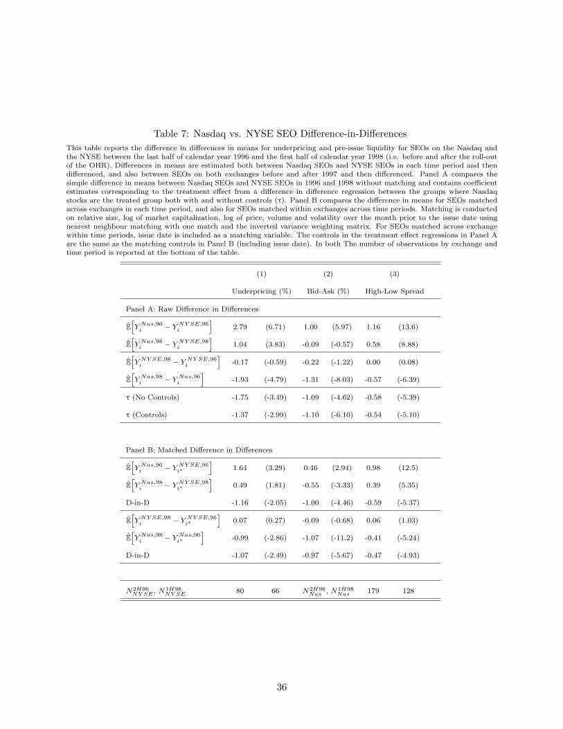
Table 7: Nasdaq vs. NYSE SEO Difference-in-Differences

This table reports the difference in differences in means for underpricing and pre-issue liquidity for SEOs on the Nasdaq andthe NYSE between the last half of calendar year 1996 and the first half of calendar year 1998 (i.e. before and after the roll-outof the OHR). Differences in means are estimated both between Nasdaq SEOs and NYSE SEOs in each time period and thendifferenced, and also between SEOs on both exchanges before and after 1997 and then differenced. Panel A compares thesimple difference in means between Nasdaq SEOs and NYSE SEOs in 1996 and 1998 without matching and contains coefficientestimates corresponding to the treatment effect from a difference in difference regression between the groups where Nasdaqstocks are the treated group both with and without controls (τ). Panel B compares the difference in means for SEOs matchedacross exchanges in each time period, and also for SEOs matched within exchanges across time periods. Matching is conductedon relative size, log of market capitalization, log of price, volume and volatility over the month prior to the issue date usingnearest neighbour matching with one match and the inverted variance weighting matrix. For SEOs matched across exchangewithin time periods, issue date is included as a matching variable. The controls in the treatment effect regressions in Panel Aare the same as the matching controls in Panel B (including issue date). In both The number of observations by exchange andtime period is reported at the bottom of the table.

(1) (2) (3)

Underpricing (%) Bid-Ask (%) High-Low Spread

Panel A: Raw Difference in Differences

E[Y Nas,96i − Y NY SE,96

i

]2.79 (6.71) 1.00 (5.97) 1.16 (13.6)

E[Y Nas,98i − Y NY SE,98

i

]1.04 (3.83) -0.09 (-0.57) 0.58 (8.88)

E[Y NY SE,98i − Y NY SE,96

i

]-0.17 (-0.59) -0.22 (-1.22) 0.00 (0.08)

E[Y Nas,98i − Y Nas,96

i

]-1.93 (-4.79) -1.31 (-8.03) -0.57 (-6.39)

τ (No Controls) -1.75 (-3.49) -1.09 (-4.62) -0.58 (-5.39)

τ (Controls) -1.37 (-2.99) -1.10 (-6.10) -0.54 (-5.10)

Panel B: Matched Difference in Differences

E[Y Nas,96i − Y NY SE,96

i∗

]1.64 (3.29) 0.46 (2.94) 0.98 (12.5)

E[Y Nas,98i − Y NY SE,98

i∗

]0.49 (1.81) -0.55 (-3.33) 0.39 (5.35)

D-in-D -1.16 (-2.05) -1.00 (-4.46) -0.59 (-5.37)

E[Y NY SE,98i − Y NY SE,96

i∗

]0.07 (0.27) -0.09 (-0.68) 0.06 (1.03)

E[Y Nas,98i − Y Nas,96

i∗

]-0.99 (-2.86) -1.07 (-11.2) -0.41 (-5.24)

D-in-D -1.07 (-2.49) -0.97 (-5.67) -0.47 (-4.93)

N2H96NY SE , N1H98

NY SE 80 66 N2H96Nas , N1H98

Nas 179 128

36

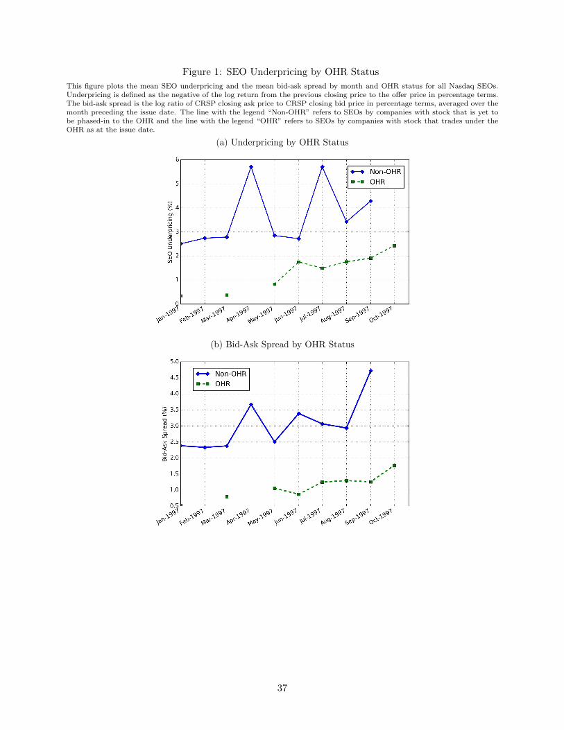
Figure 1: SEO Underpricing by OHR Status

This figure plots the mean SEO underpricing and the mean bid-ask spread by month and OHR status for all Nasdaq SEOs.Underpricing is defined as the negative of the log return from the previous closing price to the offer price in percentage terms.The bid-ask spread is the log ratio of CRSP closing ask price to CRSP closing bid price in percentage terms, averaged over themonth preceding the issue date. The line with the legend “Non-OHR” refers to SEOs by companies with stock that is yet tobe phased-in to the OHR and the line with the legend “OHR” refers to SEOs by companies with stock that trades under theOHR as at the issue date.

(a) Underpricing by OHR Status

(b) Bid-Ask Spread by OHR Status

37

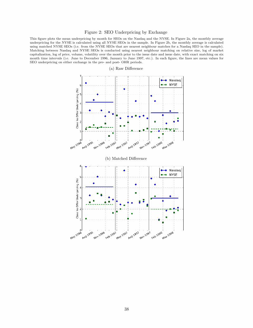
Figure 2: SEO Underpricing by Exchange

This figure plots the mean underpricing by month for SEOs on the Nasdaq and the NYSE. In Figure 2a, the monthly averageunderpricing for the NYSE is calculated using all NYSE SEOs in the sample. In Figure 2b, the monthly average is calculatedusing matched NYSE SEOs (i.e. from the NYSE SEOs that are nearest neighbour matches for a Nasdaq SEO in the sample).Matching between Nasdaq and NYSE SEOs is conducted using nearest neighbour matching on relative size, log of marketcapitalization, log of price, volume, volatility over the month prior to the issue date and issue date, with exact matching on sixmonth time intervals (i.e. June to December 1996, January to June 1997, etc.). In each figure, the lines are mean values forSEO underpricing on either exchange in the pre- and post- OHR periods.

(a) Raw Difference

(b) Matched Difference

38

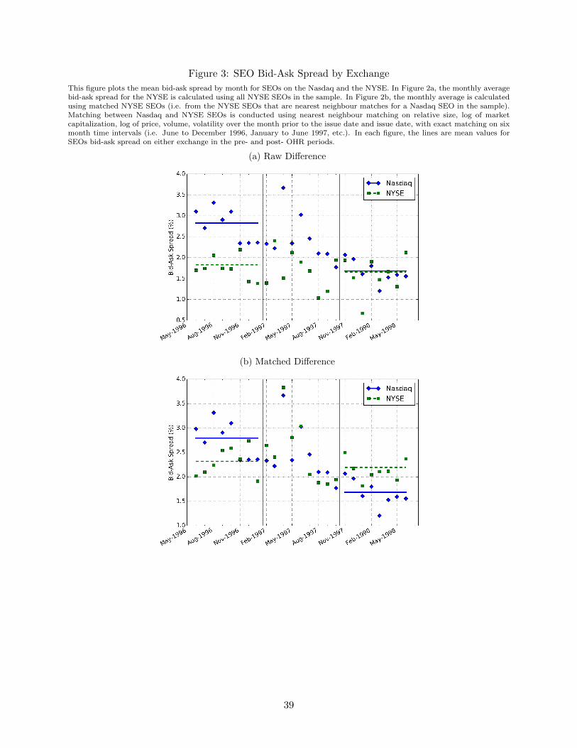
Figure 3: SEO Bid-Ask Spread by Exchange

This figure plots the mean bid-ask spread by month for SEOs on the Nasdaq and the NYSE. In Figure 2a, the monthly averagebid-ask spread for the NYSE is calculated using all NYSE SEOs in the sample. In Figure 2b, the monthly average is calculatedusing matched NYSE SEOs (i.e. from the NYSE SEOs that are nearest neighbour matches for a Nasdaq SEO in the sample).Matching between Nasdaq and NYSE SEOs is conducted using nearest neighbour matching on relative size, log of marketcapitalization, log of price, volume, volatility over the month prior to the issue date and issue date, with exact matching on sixmonth time intervals (i.e. June to December 1996, January to June 1997, etc.). In each figure, the lines are mean values forSEOs bid-ask spread on either exchange in the pre- and post- OHR periods.

(a) Raw Difference

(b) Matched Difference

39

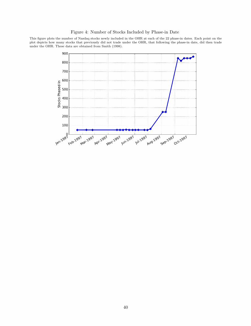
Figure 4: Number of Stocks Included by Phase-in Date

This figure plots the number of Nasdaq stocks newly included in the OHR at each of the 22 phase-in dates. Each point on theplot depicts how many stocks that previously did not trade under the OHR, that following the phase-in date, did then tradeunder the OHR. These data are obtained from Smith (1998).

40

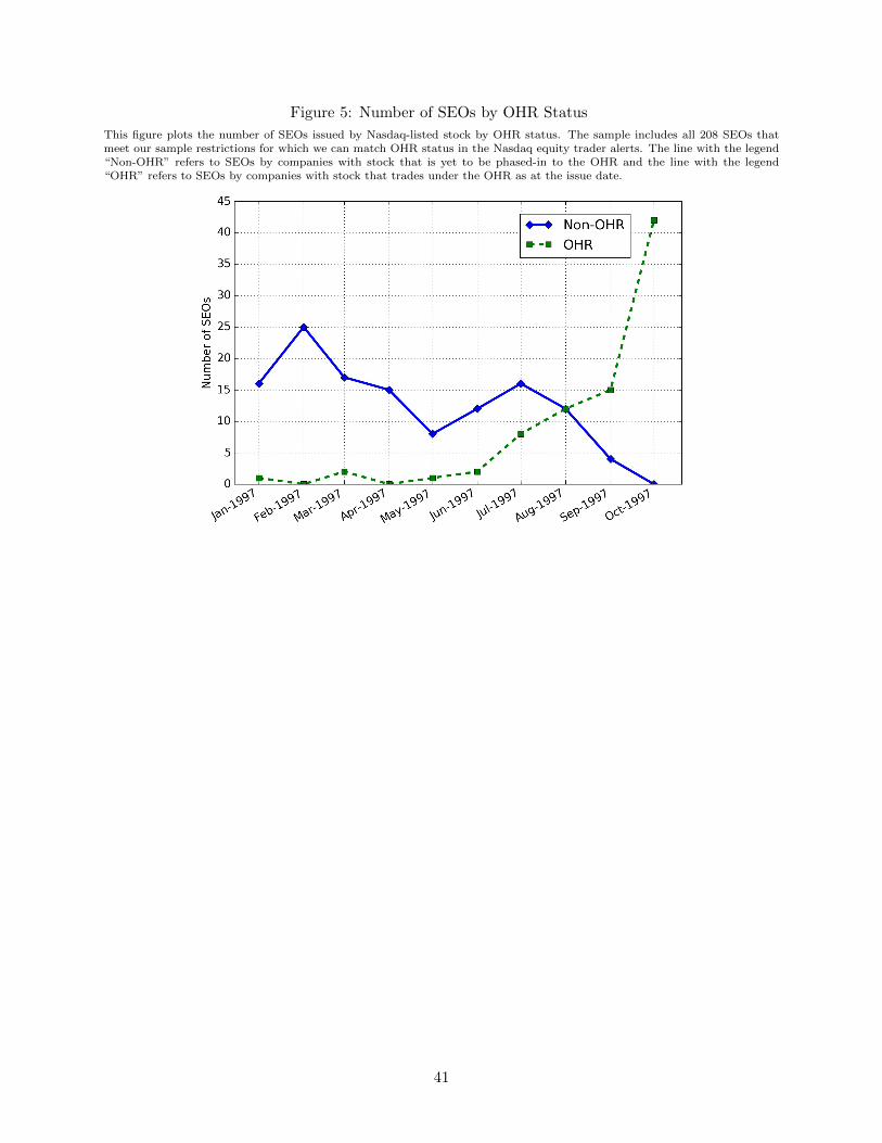
Figure 5: Number of SEOs by OHR Status

This figure plots the number of SEOs issued by Nasdaq-listed stock by OHR status. The sample includes all 208 SEOs thatmeet our sample restrictions for which we can match OHR status in the Nasdaq equity trader alerts. The line with the legend“Non-OHR” refers to SEOs by companies with stock that is yet to be phased-in to the OHR and the line with the legend“OHR” refers to SEOs by companies with stock that trades under the OHR as at the issue date.

41

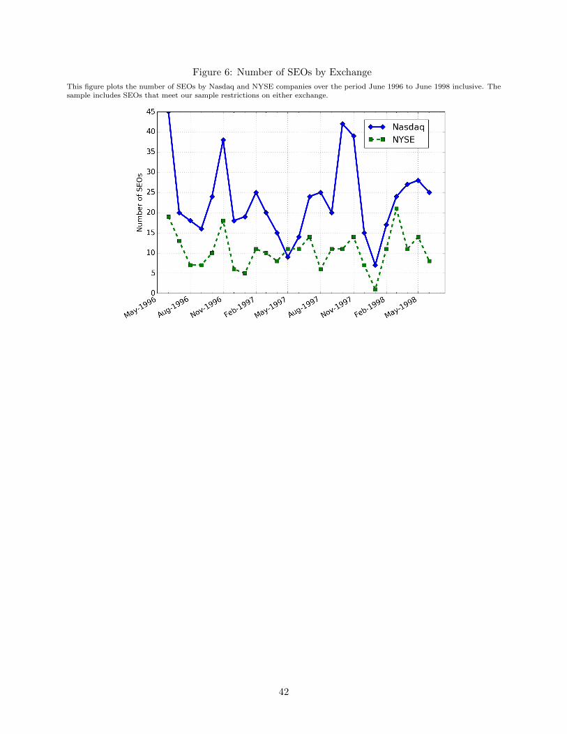
Figure 6: Number of SEOs by Exchange

This figure plots the number of SEOs by Nasdaq and NYSE companies over the period June 1996 to June 1998 inclusive. Thesample includes SEOs that meet our sample restrictions on either exchange.

42