does employee happiness have an impact on productivity?

Saïd Business School Research Papers

Saïd Business School WP 2019-13 The Saïd Business School’s working paper series aims to provide early access to high-quality and rigorous academic research. Oxford Saïd’s working papers reflect a commitment to excellence, and an interdisciplinary scope that is appropriate to a business school embedded in one of the world’s major research universities. This paper is authored or co-authored by Oxford Saïd faculty. It is circulated for comment and discussion only. Contents should be considered preliminary, and are not to be quoted or reproduced without the author’s permission.

Does Employee Happiness Have an Impact on Productivity?

Clement S. Bellet Erasmus University Rotterdam

Jan-Emmanuel De Neve Saïd Business School, University of Oxford

George Ward Massachusetts Institute of Technology

October 2019

Electronic copy available at: https://ssrn.com/abstract=3470734

Does Employee Happiness Have an

Impact on Productivity?∗

Clement S. Bellet

Erasmus University Rotterdam

Jan-Emmanuel De Neve

University of Oxford

George Ward

Massachusetts Institute of Technology

October 14, 2019

Abstract

This article provides quasi-experimental evidence on the relationship between employee

happiness and productivity in the field. We study the universe of call center sales workers at

British Telecom (BT), one of the United Kingdom’s largest private employers. We measure

their happiness over a 6 month period using a novel weekly survey instrument, and link

these reports with highly detailed administrative data on workplace behaviors and various

measures of employee performance. We show that workers make around 13% more sales in

weeks where they report being happy compared to weeks when they are unhappy. Exploiting

exogenous variation in employee happiness arising from weather shocks local to each of the 11

call centers, we document a strong causal effect of happiness on labor productivity. These

effects are driven by workers making more calls per hour, adhering more closely to their

workflow schedule, and converting more calls into sales when they are happier. No effects

are found in our setting of happiness on various measures of high-frequency labor supply

such as attendance and break-taking.

JEL: D03; J24; M5; I31

∗We thank Alex Bryson, Ed Diener, Alex Edmans, Paul Frijters, Sergei Guriev, John Helliwell, Erin Kelly, TomKochan, Richard Layard, Armando Meier, Robert Metcalfe, Michael Norton, Paul Osterman, Alexandra Roulet,Mark Stabile, Andrew Stephen, John Van Reenen, and Ashley Whillans for helpful comments on manuscriptdrafts. We also thank seminar participants at Oxford, MIT, London School of Economics, and Paris School ofEconomics for helpful discussions. We are grateful to British Telecom for for the opportunity to design and runthis study and for providing access to their administrative data. We also thank Butterfly AI for their technicalsupport in implementing the employee survey. De Neve is a research advisor to Butterfly AI. Correspondence:George Ward, MIT Sloan, 100 Main Street, Cambridge MA. Email: [email protected].

1


1 Introduction

What explains the large differences in labor productivity that are typically observed between

firms and individuals? Historically, theoretical and empirical work seeking to understand such

differentials has mostly focused on monetary aspects of motivation (e.g. Lazear, 2000). However,

a more recent stream of economic research has begun to broaden this focus to also include non-

monetary aspects of work, such as intrinsic motivation, social preferences, meaningfulness of

tasks, and social comparisons (e.g. Benabou and Tirole, 2003; Cassar and Meier, 2018; DellaV-

igna and Pope, 2017; Gneezy and Rustichini, 2000; Ichniowski and Shaw, 2003). In this paper,

we add to this growing literature by studying the productivity effects of a typically-overlooked

aspect of workers’ lives: their day-to-day happiness.

A recent trend has seen a growing number of employers at least claiming to care about

the happiness of their employees, and beginning to invest in management practices and services

aimed at creating and maintaining a happy workforce.1 At least one reason for this is the expec-

tation that happier workers will be more productive in their jobs.2 However, it remains unclear

whether this belief is based on sound empirical evidence or is, rather, a case of “management

mythology”.

We build on a long history of work, largely outside of economics, on employee well-being and

performance. A large initial stream of research examined the association between measures of

self-reported job satisfaction and worker performance, typically in field settings, and has gener-

ally found a modest positive correlation between the two (see Judge et al., 2001, for a review).

However, there is a general lack of causal research on the issue, and the best existing evidence

relies principally on within-worker estimates. A more recent stream of research—arising largely

out of cognitive psychology—has moved away from evaluative assessments of employee satisfac-

tion, in order to study people’s affective or emotional states in the workplace (Brief and Weiss,

2002; Tenney et al., 2016). One benefit of studying emotional states is that they are more

readily manipulable in laboratory settings, allowing for more clearly causal research designs. A

recent pioneering paper in economics, for example, influences happiness in a laboratory setting

to show a robust causal effect on a stylized, piece-rate productivity task (Oswald et al., 2015).3

However, it remains unclear whether these effects translate into real-world employment settings.

In this paper, we present evidence of a causal effect of workers’ week-to-week happiness on

their productivity, in a field context at one of the United Kingdom’s largest private employers.

We study the universe of around 1,800 sales workers at British Telecom (BT), a large telecom-

munications firm in the UK. Employees are distributed across 11 call centers, where their job is

predominantly to take incoming calls from new and existing customers, and seek to sell them

various products such as broadband internet contracts, cell and landline phone deals, and tele-

vision packages. We observe the happiness of these workers on a weekly basis over a six month

period. We match this self-reported happiness data to detailed administrative data on a number

1Companies such as Google or Zappos, for example, have even appointed “Chief Happiness Officers” to thisend (Knowles, 2015).

2Other motivations may also include a desire to attract and retain high quality workers, the enhancement offirms’ reputation among customers, as well as concerns to do with corporate social responsibility.

3For earlier work in psychology showing the effects of positive mood on task performance in a non-incentivizedsetting, see Erez and Isen (2002). See also Isen and Reeve (2005).

2


of workplace behaviors and performance outcomes. Whereas much of the prior literature on

worker well-being and performance has been forced to rely on subjective outcomes—such as

managerial performance evaluations—the benefit of studying a call center population is that

we are able to study a range of objective, quantitative performance metrics that are measured

routinely by the firm. For our main outcome measure, we focus on the number of weekly sales

made by each employee. In order to investigate channels through which any effect of happiness

may translate into sales, we also study fine-grained measures of labor productivity, namely i)

minutes per call, ii) the percentage of calls converted to sales, and iii) the extent to which

workers “adhere” to their scheduled workflow.

The use of high-frequency panel data allows us to purge from our estimates any unobserved

heterogeneity between workers. However, there remain reasons to believe our within-worker

estimates could still be biased. First, our survey measure of happiness may be a noisy measure

of workers’ happiness, and this measurement error is likely to bias any estimate downward.

Second, there is a concern of reverse causation, and here the direction of the bias is theoretically

ambiguous. On the one hand, strong performance could increase the mood of workers if they

derive enjoyment from the success of making sales. But on the other hand, if tasks are not

in themselves enjoyable or fulfilling then doing more of them could produce unhappiness.4 We

present evidence more in line with the latter — suggesting that in more routine work settings

the causal effect of happiness on performance is likely to be greater in magnitude than the

initially observed within-worker association.

We study adverse local weather shocks in order to set up a natural experiment wherein we

are able to estimate the causal effect of happiness on productivity. We instrument for employees’

weekly happiness using local weather conditions. Using weather station data local to each of

our 11 call centers we construct a Bad Weather Index, which is the weekly total incidence of

fog, rain and snow close to each call center. This has a strong (“first-stage”) negative effect on

worker happiness, which we show ultimately leads to fewer weekly sales in two-stage IV models.

Our key identifying assumption is that weather patterns have an effect on sales only through

variation in worker happiness. We explore in detail at least two principal threats to this as-

sumption. First, there is a possibility that weather will also affect product demand, either

directly or indirectly through the mood of customers. It is worth noting here that demand is

national, and that calls are allocated to call centers based on call type and operator availability.

In all of our models, we include both worker and week fixed effects, such that our key piece

of identifying variation in the data comes from differences across call centers (which are very

widely dispersed geographically across 3 countries, from the south coast of England to the north

of Scotland) within any given week, and not from seasonal movements in national weather from

week-to-week.

Second, it may be that weather shocks affect how much people work. For example, poor

weather could influence commuting patterns, or induce sickness among workers causing them

to attend less. Equally, it weather could affect the opportunity cost of leisure compared to work

(see Connolly, 2008), and have effects on attendance. One of the key benefits of studying workers

in a call center setting is that employees enjoy very little—if any—discretion over their day-to-

4Equally, higher volumes of work related to making more sales could also lead to stress.

3


day work hours, making it an ideal population in which to cleanly measure labor productivity

effects.

In line with this, when examining channels, we find null effects on various fine-grained

measures of labor supply such as attendance, sickness leave, overtime, or length of paid and

unpaid breaks. Instead, leveraging detailed data on high-frequency labor productivity, we show

that the effect of happiness on sales is driven largely by employees both working faster (i.e.

making more calls per hour) and also converting more of their calls into sales during weeks

when they feel happier. The latter channel suggests that the effects of happiness are likely to be

strongest in service industry settings, where work is directly customer-facing. Happiness may

in this sense be beneficial to people’s social skills, the importance of which have been shown to

be increasing in the labor market (Deming, 2017). Underscoring the importance of happiness

as an aid to social skills, we show that the effects are greater for upgrade and re-contracting

sales—where there is more leeway for inter-personal connection, persuasion, and negotiation—

than they are for more routine order-taking. We also discuss the contribution of alternative

psychological mechanisms such as intrinsic motivation and cognitive processing.

The findings contribute to various strands of research in economics, psychology, sociology,

and industrial relations. First, as noted above, the analysis relates directly to a large and

long-standing literature in economics on the determinants of productivity (Syverson, 2011).

Second, the results contribute to a large body of work outside economics, which has a

long history of examining the relationship between employee well-being and performance. In

studying well-being in a field setting, our work is closely related to research on job satisfaction

and performance. But in studying a measure of positive affect, our findings are also closely

related to a largely more laboratory-based literature on emotional states in determining work-

related outcomes (see Walsh et al., 2018, and citations within for an extensive review of the

evidence arising from both streams of work).5

Third, our findings provide micro-foundation for work showing that firms listed in the “100

Best Companies To Work For In America” outperform industry benchmarks in terms of long-

run stock returns (Edmans, 2011), as well as for research suggesting a positive link between

firm-level employee satisfaction and financial performance (Bockerman and Ilmakunnas, 2012;

Bryson et al., 2017; Krekel et al., 2019). Fourth, and relatedly, the findings are in line with an

experimental literature at the individual level, largely in psychology, showing in non-incentivized

laboratory settings that induced happiness has effects on processes like motivation, cognitive

flexibility, negotiation, and problem solving skills (see Isen, 2001, for a review).

Fifth, the results contribute to work in economics that implies the existence of mood effects

on workplace behaviors, but is unable to measure them directly. Heyes and Saberian (2019)

show, for example, that temperature has significant effects on the decision-making of judges in

high-stakes court cases, while work by Eren and Mocan (2018) suggests that judges’ decisions can

be swayed by college football results. Equally, behavior in stock markets is affected by sunshine

and daylight hours (Hirshleifer and Shumway, 2003; Kamstra et al., 2003) and national soccer

results (Edmans et al., 2007). While none of these papers is able to measure mood directly,

5In a paper relatively close in nature to ours, Rothbard and Wilk (2011) study the mood and performance ofa sample of 29 call center workers in an insurance firm, and present within-worker estimates of the relationshipbetween affect and task performance.

4


all explicitly tell a story in which emotional states causally affect workplace behaviors. Our

analysis contributes to this literature by more directly measuring the effects of happiness and

unhappiness on performance.

Finally, our study also ties in to an emerging field-experimental literature showing that the

improvement of management practices can have simultaneously positive impacts on i) employee

happiness and satisfaction as well ii) as productivity (e.g. Gosnell et al., 2019). Bloom et al.

(2014) show, for example, that allowing call center employees to work from home improves their

productivity while also enhancing happiness and satisfaction, and an intervention by Breza

et al. (2017) shows that pay inequality has negative effects on morale while also depressing

productivity.6 Each of these papers suggests that employee happiness may be one channel

through which workplace organization feeds through to productivity. In this paper, we isolate

this channel more clearly in order to show a positive causal relationship between happiness and

employee performance.

2 Data and Institutional Setting

We collect data from a large telecommunications company based in the United Kingdom. We

focus our analysis on the firm’s 11 call centers located across England, Scotland and Wales that

have a large number of workers concentrating predominantly on sales. We use administrative

data obtained from the firm on worker characteristics, work schedules and productivity, and

combine these data with an original survey instrument we implemented to measure workers’

psychological well-being over a six month period.

2.1 Psychological Well-Being Survey

The use of “happiness” data in economics has grown substantially over the past decade (see,

e.g, Aghion et al., 2016; Benjamin et al., 2012; Haushofer and Shapiro, 2016; Kahneman et al.,

2004; Luttmer, 2005). Subjective well-being is typically divided into two separate components

that measure i) how people feel as well as ii) how they think about their lives (Kahneman and

Krueger, 2006).7 Evaluative measures of psychological well-being typically comprise answers

to global, cognitive judgements like the extent to which people are satisfied with their job or

their life overall. Affective measures of well-being – which are often also referred to as ‘hedonic’

or ‘experienced’ measures – refer, on the other hand, to the extent to which people experience

positive and negative emotional states (like happiness, enjoyment, stress and worry) in the

course of their day-to-day lives.

Whereas much of the existing literature on well-being in the workplace focuses on evaluative

measures of job satisfaction, which are typically slow-moving overall cognitive assessments, we

focus instead on employees’ experienced well-being as it varies week-to-week. In doing so,

we build on a small experimental literature that manipulates positive and negative affect in

6Similarly, Moen et al. (2017) show that improving worker autonomy has a positive effect on well-being andalso decreases turnover (see also Moen et al., 2016). The authors are unable, however, to observe productivityin their IT firm setting.

7A third component is increasingly also identified, which comprises meaningfulness or “eudaemonia” (see, e.g.,Ariely et al., 2008).

5


Figure 1: Happiness Survey Email

Note: Screenshot of the happiness survey, which was sent weekly over a six month period to all workers. Respon-dents had to click a face within the email for their response to be registered. See text for more details.

the laboratory in order to examine effects on economic outcomes like productivity (Oswald

et al., 2015), time preferences (Ifcher and Zarghamee, 2011), and behavior in ultimatum and

trust games (Capra, 2004). For ease of exposition, we use the terms ‘happiness’, ‘positive

mood’, ‘affect’, ‘affective state’, ‘emotional well-being’ and ‘emotional state’ interchangeably

throughout the paper.8

In designing our survey instrument, the firm followed the OECD’s measurement guidelines,

which they provide largely for the benefit of national statistical offices seeking to measure pop-

ulation subjective well-being for policy purposes (see OECD, 2013).9 Employees were asked

“Overall, how happy did you feel this week?”.10 Following Kunin (1955) and decades of sub-

sequent work in the psychological literature, we offer five response categories as a Faces Scale

that ranges from very sad to very happy androgynous faces.11 The use of faces in this way is

both intuitive to respondents, and is also known to strongly pick up the affective component of

well-being questions (Fisher, 2000).

The question was asked on a weekly basis for six months, beginning in July 2017. The

survey was sent by email on Thursday afternoon, and is shown in Figure 1. It is important

to note that we measured happiness at the end of the week, and asked employees about their

happiness during that particular week. This allows us to link happiness reports and work

outcomes over the same corresponding time period. An alternative option would be to ask

8Feeling states are typically categorized into moods and emotions. While emotions are discrete short-runreactions, usually to a specific stimulus, moods are more general positive or negative feeling states (Frijda, 1986).A related literature considers the effects of discrete emotions, rather than mood, on economic behavior (seeLoewenstein, 2000).

9For a full discussion of the issues surrounding the measurement of subjective well-being, as well as a detailedaccount of the various ways in which the validity and reliability of such measures have been tested, see OECD(2013). See also Krueger and Stone (2014) and Krueger and Schkade (2008). The OECD reports that well-beingmeasures are now being regularly collected in over 20 countries, many of which are also using them systematicallyin the policymaking process (Durand, 2018).

10This is (by design) very close in wording to the standard happiness question asked by the UK government’sOffice for National Statistics (ONS) in all of its main household and labor force surveys. The ONS questionasks: “On a 0-10 scale where 0 is not at all happy and 10 is completely happy, overall, how happy did you feelyesterday?” (see Dolan et al., 2011).

11One notable issue with the use of faces in this way is that people – men and women, in particular – havebeen shown to interpret the neutral face in different ways (see, e.g., Elfering and Grebner, 2010). Since our mainspecifications use individual fixed effects and look within-workers over time, such issues of response style aremuch less of a concern here.

6


employees at the start of the week, which would give a clearer temporal ordering between

happiness and subsequent outcomes. However, this would come at the expense of not knowing

workers’ happiness during the period where they are actually working on those sales. Our use

of happiness and sales measures that are temporally concurrent thus has significant benefits,

but the contemporaneous nature of our happiness and sales measures underlines the need for

an instrumental variables strategy in order to deal with potential issues of endogeneity.

In order to reduce the onerousness of the data collection on employees, and in doing so

ensure as high a response rate as possible, the survey was a single-item question that could be

answered simply by clicking an answer from within the email. Specifically, there was no need

to click on a link through to a further webpage (as is typically the case with emailed surveys)

in order to register a response. Workers were assured that their individual happiness responses

would not be shared with the firm’s management. Workers were also offered the opportunity

to opt-out of the study at any time, via a simple email click-through.

The responses provide us with a weekly, ordinal measure of affective well-being. The distri-

bution of responses is shown in panel (a) of Figure 2. Although we assign a numerical value to

each of the responses ranging from 1 (least happy) to 5 (most happy), we are naturally hesi-

tant to cardinalize the scale into a continuous measure of happiness – and in our main initial

empirical model we introduce the response categories into our productivity equation as a set of

indicator variables.

As can be seen in Figure 2, the modal response is the least happy state. If we are to use

the scale in a continuous manner, the mean response is 2.6 with a standard deviation of 1.4 (a

full set of descriptive statistics are shown in Table A1). Importantly for our identification using

individual fixed effect models, panel (c) of Figure 2 shows that the responses vary significantly

within-workers over time during the study, suggesting that we are not simply picking up a more

static overall measure of evaluative job satisfaction.

2.2 Administrative data

We combine the survey responses with detailed individual-level administrative data from the

firm. We focus our attention on sales workers across the 11 call centers, whose job it is to sell

a variety of BT products. These predominantly consist of landline and cellphone contracts,

broadband internet contracts, and television subscription bundles. The vast majority of the

work (91% of time and 82% of tasks) carried out by the employees in the sample are incoming

calls from potential or existing customers, with the remainder consisting of outgoing calls (4% of

time and 12% of tasks) and “other” activities (which includes tasks such as dealing with inbound

and outbound letters, online customer chats, and incoming and outgoing SMS messaging).

Workers are observed in the data on a daily basis and are identified by their unique personal

ID as well as a time-varying team ID. Workers sit individually at desks with a computer terminal

and a telephone headset, and are clustered physically in the workspace by their team. Although

workers are organized into teams, this largely relates to the sharing of a line manager and not

to any interdependence of workflow, since the job of selling in this context is almost exclusively

an independent task with very little to no teamwork involved.

At the worker-day level we observe the number of sales, which include new sales, whether to

7


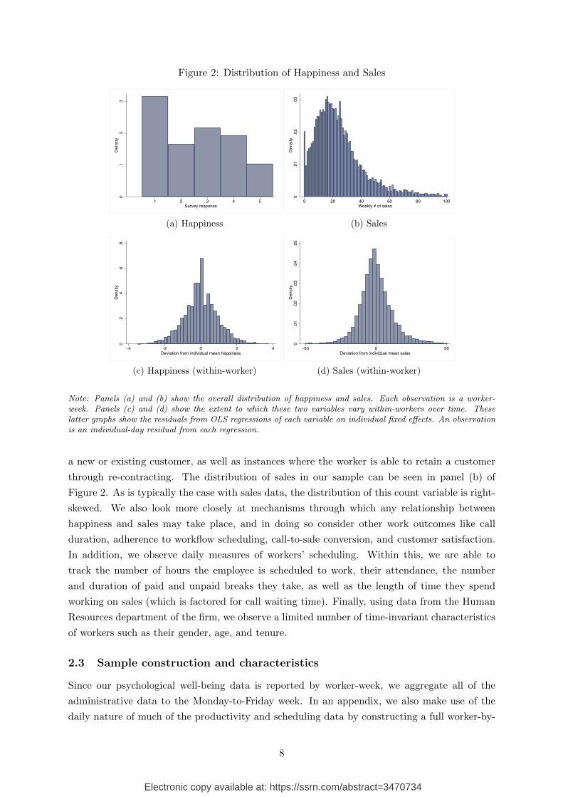
Figure 2: Distribution of Happiness and Sales

0.1

.2.3

Den

sity

1 2 3 4 5Survey response

(a) Happiness

0.0

1.0

2.0

3D

ensi

ty

0 20 40 60 80 100Weekly # of sales

(b) Sales

0.2

.4.6

.8D

ensi

ty

-4 -2 0 2 4Deviation from individual mean happiness

(c) Happiness (within-worker)

0.0

1.0

2.0

3.0

4.0

5D

ensi

ty

-50 0 50Deviation from individual mean sales

(d) Sales (within-worker)

Note: Panels (a) and (b) show the overall distribution of happiness and sales. Each observation is a worker-week. Panels (c) and (d) show the extent to which these two variables vary within-workers over time. Theselatter graphs show the residuals from OLS regressions of each variable on individual fixed effects. An observationis an individual-day residual from each regression.

a new or existing customer, as well as instances where the worker is able to retain a customer

through re-contracting. The distribution of sales in our sample can be seen in panel (b) of

Figure 2. As is typically the case with sales data, the distribution of this count variable is right-

skewed. We also look more closely at mechanisms through which any relationship between

happiness and sales may take place, and in doing so consider other work outcomes like call

duration, adherence to workflow scheduling, call-to-sale conversion, and customer satisfaction.

In addition, we observe daily measures of workers’ scheduling. Within this, we are able to

track the number of hours the employee is scheduled to work, their attendance, the number

and duration of paid and unpaid breaks they take, as well as the length of time they spend

working on sales (which is factored for call waiting time). Finally, using data from the Human

Resources department of the firm, we observe a limited number of time-invariant characteristics

of workers such as their gender, age, and tenure.

2.3 Sample construction and characteristics

Since our psychological well-being data is reported by worker-week, we aggregate all of the

administrative data to the Monday-to-Friday week. In an appendix, we also make use of the

daily nature of much of the productivity and scheduling data by constructing a full worker-by-

8


day dataset and assuming happiness to be constant throughout the days of that week (given

that the question asks them specifically how happy they have felt overall during the week).

We observe 1,793 sales workers, distributed across 11 different call centers (for a map of the

spatial distribution of these call centers, see Figure 4). All of these workers were invited to take

part in the study and were sent weekly psychological well-being surveys. Of these employees,

1,438 (around 80%) participated by answering at least one survey over the subsequent 6 months.

All of this cohort of workers were sent a weekly email, unless they had since left the organization

(in which case their email survey is recorded as “bounced”). We do not follow any workers who

subsequently joined the firm after the first week of the study. In the supplementary material, we

assess the extent to which observable demographic characteristics and workplace performance

are able to predict i) participation in the study, on the extensive margin (Table S1) and ii) the

number of survey waves answered if the worker did participate, on the intensive margin (Table

S2). Importantly, neither participation in the study nor frequency of response are significantly

related to the average weekly number of sales made by workers during the course of the study.

Mean hours of selling time is positively predictive of the number of response waves – an extra

hour of mean daily sales time is associated with around a 2% increase in the number of waves

responded.

We drop any participants who responded to only one survey wave, since we rely principally

on within-worker variation over time in our main analysis. Also dropped from the analysis

are observations that lead to statistical separation in our main individual and week fixed-effect

Poisson models. This leaves us with a final sample of 1,161 employees. Summary statistics for

this final sample are shown in Table A1. Around 57% are male, and the modal age category is

26-30 (with over 60% of the sample being between 21 and 35 years old). Mean tenure in the

firm is about 5 years, with a large standard deviation of 7 years. Half of the workforce in our

sample has been in this position for less than 2 years, and around 7% of the sample experienced

turnover during the 6 months – either leaving of their own accord or having their employment

terminated. Conditional on participating in the study, workers responded to a mean of 10.3

waves (with an SD of 7.1). The weekly response rate of workers who participated was on average

around 37%.

Using our final sample of workers, we do not observe a fully balanced worker-week panel

since we are restricted by non-response to the happiness survey instrument. Moreover, there is

a significant concern that non-response to the survey is unlikely to occur randomly, and may

indeed relate to our main variables of interest in ways likely to bias our estimates. For example,

it may be that a worker does not respond in a given week because she is either too happy or

miserable to spend time reading the email, or alternatively because she is too busy making

sales. In Table S3 we regress a dummy for having responded to the survey in a given week on a

number of time-varying observables like sales, selling time, and team average happiness (as well

as a set of individual and week fixed effects). Reassuringly, neither weekly sales performance

nor team average happiness (minus the focal worker) is significantly related to non-response

within-individuals over time. It is, however, positively related to the number of hours worked

during the week, suggesting that workers are less likely to respond during weeks in which they

are scheduled to work less.

9


Figure 3: Within-worker association of happiness and sales

Note: Coefficients and 95% confidence intervals shown from a poisson model in which the number of sales areregressed on a series of happiness dummies, a full set of individual and time fixed effects, as well as schedulingcontrols. Full model is reported in Table A2.

3 Results

3.1 Within-worker estimates

We are interested in whether workers’ self-reported psychological well-being has any causal

impact on their weekly performance at work. We focus on sales workers so that our preferred

performance measure is the worker’s number of weekly sales. We estimate a within-worker

productivity equation, such that

E[Sijt|Hijt, Xijt] = exp{βHijt + γXijt + νi + τt

}(1)

where Sijt corresponds to the number of weekly sales for worker i in call center j during

week t and Hijt is her reported happiness during that same period t. Worker fixed effects νi

capture any individual-specific characteristic that does not change over time, and τt is a time

fixed effect partialing out any shocks that may affect both well-being and sales. Finally, we

include a vector of controls Xijt for two major work schedule variables that may vary over time

and across workers, namely the total number of selling hours during week t (and its squared

value), and the fraction of time spent at work in the week on internal training.

We estimate equation (1) with a Poisson quasi-maximum likelihood model. The Poisson

model is particularly relevant for count data, and also makes the interpretation of β intuitive,

as it can be interpreted in terms of a percent change in number of sales per hour. A linear

specification using logged sales per hour, which leads us to lose around 2% of our sample size

due to observations with zero sales, is reported in Table S13 and gives similar estimates.

We show the results of this empirical model in Figure 3 (for full reporting of this model, see

10


Figure 4: Spatial Distribution of Call Centers

Note: Map shows the location of the 11 call centers in the study, as well as the number of sales workers in each.

Table A2). We omit the neutral third category of happiness from the regression, and show the

association of happiness and unhappiness in relation to this. Each of these four (unhappiness)

indicators enters significantly into the productivity equation. As can be seen, being in the most

happy state (as compared to a neutral emotional state) is associated with around a 6% rise in

weekly sales. Being in a negative emotional state (as compared to the neutral) is associated with

around an 7% decrease in weekly sales. There is, thus, a slight asymmetry in the association

of happiness and unhappiness with sales. Comparing weeks when workers report being very

unhappy with weeks where they are very happy, the difference in sales is around 13%.

3.2 IV estimates

One major empirical concern is that, even within-workers over time, a change in subjective

well-being may be endogenous to performance. In particular, we see two (opposing) major

ways in which reverse causality may bias our coefficients. First, more productive workers can

get compensated for their higher performance through financial incentives, or non-monetary

rewards from their colleagues or managers, or simply enjoyment. This alone could explain

their higher reported well-being, in which case the coefficient will be biased upward. Second,

and conversely, higher productivity and being over-worked can lead to higher levels of stress

or anxiety, which are both highly likely to be negatively correlated with happiness. Equally,

doing more work may simply be more unenjoyable. In this case, the coefficient will be biased

downward.

Our main strategy to deal with the endogeneity of Hijt is to rely on instrumental variables

Zijt that are correlated with the latter, but are independent of sales. In our case, the first stage

is:

Hijt = ωZjt + ΓXijt + νi + τt + ηijt (2)

11


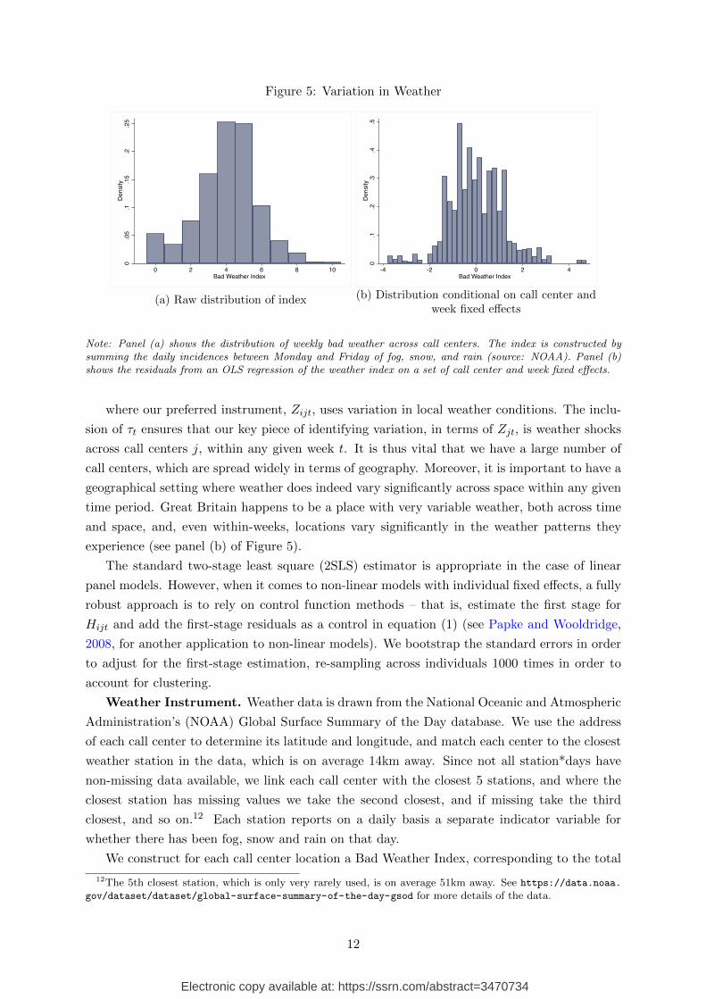
Figure 5: Variation in Weather

0.0

5.1

.15

.2.2

5D

ensi

ty

0 2 4 6 8 10Bad Weather Index

(a) Raw distribution of index

0.1

.2.3

.4.5

Den

sity

-4 -2 0 2 4Bad Weather Index

(b) Distribution conditional on call center andweek fixed effects

Note: Panel (a) shows the distribution of weekly bad weather across call centers. The index is constructed bysumming the daily incidences between Monday and Friday of fog, snow, and rain (source: NOAA). Panel (b)shows the residuals from an OLS regression of the weather index on a set of call center and week fixed effects.

where our preferred instrument, Zijt, uses variation in local weather conditions. The inclu-

sion of τt ensures that our key piece of identifying variation, in terms of Zjt, is weather shocks

across call centers j, within any given week t. It is thus vital that we have a large number of

call centers, which are spread widely in terms of geography. Moreover, it is important to have a

geographical setting where weather does indeed vary significantly across space within any given

time period. Great Britain happens to be a place with very variable weather, both across time

and space, and, even within-weeks, locations vary significantly in the weather patterns they

experience (see panel (b) of Figure 5).

The standard two-stage least square (2SLS) estimator is appropriate in the case of linear

panel models. However, when it comes to non-linear models with individual fixed effects, a fully

robust approach is to rely on control function methods – that is, estimate the first stage for

Hijt and add the first-stage residuals as a control in equation (1) (see Papke and Wooldridge,

2008, for another application to non-linear models). We bootstrap the standard errors in order

to adjust for the first-stage estimation, re-sampling across individuals 1000 times in order to

account for clustering.

Weather Instrument. Weather data is drawn from the National Oceanic and Atmospheric

Administration’s (NOAA) Global Surface Summary of the Day database. We use the address

of each call center to determine its latitude and longitude, and match each center to the closest

weather station in the data, which is on average 14km away. Since not all station*days have

non-missing data available, we link each call center with the closest 5 stations, and where the

closest station has missing values we take the second closest, and if missing take the third

closest, and so on.12 Each station reports on a daily basis a separate indicator variable for

whether there has been fog, snow and rain on that day.

We construct for each call center location a Bad Weather Index, corresponding to the total

12The 5th closest station, which is only very rarely used, is on average 51km away. See https://data.noaa.

gov/dataset/dataset/global-surface-summary-of-the-day-gsod for more details of the data.

12


https://data.noaa.gov/dataset/dataset/global-surface-summary-of-the-day-gsod

https://data.noaa.gov/dataset/dataset/global-surface-summary-of-the-day-gsod

Figure 6: Weather IV First Stage

Note: Figure shows the relationship between bad weather and happiness, adjusting for individual and week fixedeffects as well as the full set of further controls. Both weather and emotion are first regressed on the full set offixed effects and controls. The residuals from these regressions are binned across 40 quantiles and plotted as greydots. The blue line shows the linear fit from an OLS regression using all of the data.

number of daily incidences of fog, rain and snow during the week for which individuals reported

their happiness. If it were to rain, snow and be foggy every day of the week, the index would be

15, if it rains for 2 days and is foggy for 1 day, the index would be 3, and so on. Panel (a) Figure

5 shows how this index—which in theory could lie between 0 and 15 but in reality ranges from

0 to 10—is distributed once matched to the weekly performance data. Panel (b) shows there is

significant variation in the index, when conditioning on week and call center fixed effects.

Reduced Form. We first estimate the reduced form effects of local weather on sales

performance. Column (1) of Table 1 shows a negative effect of local adverse weather conditions

on sales performance. In addition, we show this at the daily-level: In table S9 we regress daily

sales on daily (and weekly) weather, together with a full set of individual and date fixed effects,

and our standard set of daily work schedule controls (equivalent to above). We find that poor

weather in the geographic region of the call center has a negative effect on sales performance.

One concern with our findings using the happiness survey is the threat of bias arising from

non-response, which we discussed above. Here we are able to make a further check, and show

that the effect of weather on sales is very similar for worker-days on which we have non-missing

and missing (weekly) happiness data.

First Stage. The negative impact of bad weather on well-being is now well documented

(Baylis et al., 2018; Connolly, 2013). We confirm this finding, and show in Figure 6 the first-

stage relationship between bad weather and worker happiness. As can be seen, within-workers

over time there is a clear negative relationship between adverse weather conditions and their

happiness. This model is also shown more formally in column (2) of Table 1. The F-statistic

from this linear first stage, which is around 10.5, suggests the instrument is sufficiently powerful

to be valid.

13


Table 1: Happiness and Sales Performance: IV estimates

Sales(Poisson)

Happiness(OLS)

Sales(Poisson)

(1) (2) (3)Red.-Form 1st Stage 2nd Stage

Happiness (1-5) 0.2403∗∗

(0.1032)Bad Weather Index -0.0057∗∗ -0.0247∗∗∗

(0.0026) (0.0076)

Observations 12,282 12,282 12,2821st Stage F-Stat 10.47

Notes: Columns (1) and (3) are Poisson-FE models. Column (2) reports an OLS-FE regression. Column(3) reports the second stage of a Poisson-FE control function model. Robust standard errors in parentheses,clustered on individuals in models (1) and (2). Bootstrapped standard errors reported for model (3), resamplingacross individuals to account for clustering. All models include individual and week fixed effects, work schedulecontrols, and day of response to survey. ∗p < 0.10, ∗∗p < 0.05, ∗∗∗p < 0.01.

Second Stage. The second stage regression, shown in column (3) of Table 1, suggests

a strong causal effect of happiness on sales performance. A one point increase in the 1-5

happiness leads to around a 24% increase in weekly sales. This implied estimate is higher than

in the equivalent non-instrumented analysis (see Table A2), suggesting a negative bias between

well-being and productivity. This could be due to a negative reverse causality bias, noted above,

wherein over-work leads to stress or where doing more work is simply unenjoyable in a job where

the tasks are not greatly interesting or fulfilling, or involve interacting with angry customers.

Equally, classical measurement error in our main right-hand-side variable is very likely to have

biased our initial estimates downward (a point we will return to below). If anything, the positive

effect found in the initial Poisson-FE specification should hence be seen as a lower bound to the

true causal effect.

3.3 Threats to validity of IV analysis

While the data suggest a strong first-stage, the instrument will only be valid under the condition

that weather has no direct impact on sales. We discuss three main threats to this exclusion

restriction:

Product Demand. One major concern here is that weather may also have a direct im-

pact on customer demand, or equally have an indirect effect on customer demand by affecting

customers’ mood. As noted above, it is important to note that we include week fixed effects in

the equation. Our 11 call centers are distributed across the whole of Great Britain, from the

south coast of England to the north of Scotland (see Figure 4 for a map). We are thus relying

on variation in weather across call centers within any given week, rather than on movements

in national weather conditions from week-to-week. Since calls come from various parts of the

country and are directed to call centers based on query type and operator availability, local

weather in the vicinity of the focal call center should be independent from customer demand.

Looking more directly in the data, we show in the online appendix that the number of incoming

calls to a given call center week-to-week (a proxy for demand) is not at all affected by weekly

14


weather that is local to that particular call center (See Table S10 of the online appendix).

Labor Supply: Opportunity Cost of Leisure. An additional concern is that the

presence of (in)clement weather outside may change the opportunity cost of leisure time (see

Connolly, 2008), leading workers to adjust their labor supply decisions. Relatedly, bad weather

could have direct impacts on employee’s ability to attend, or arrive on time – for example, if rain

affects their ability to commute to work. First, it is worth noting that, in our setting, workers

have very little discretion over labor supply. Work hours are scheduled by management, and

once workers are at their terminal during their scheduled hours they face calls as they come in.

Second, we note that all of our analyses are robust to the inclusion of a control for the number

of working hours done by the employee during the week (as well as other scheduling controls for

internal training time). Our effects are thus conditional on labor supply. In addition to this,

we also show directly in Table S10 that aggregate call center attendance is not associated with

local weather conditions. We further discuss labor supply effects in the channel section, and

find no effect of instrumented happiness on various fine-grained measures of labor supply.

Labor Supply: Sickness. A concern related to this is the possibility that adverse weather

conditions may cause sickness among workers, and impair their ability to attend work. We

use the fine-grained detail of our dataset to show at the call-center-by-week level that weather

conditions are not related to aggregate sickness (see Table S10).

Treatment Heterogeneity. In the presence of treatment response heterogeneity, a valid

instrument identifies a local average treatment effect (LATE), that is the effect driven by those

who comply with the treatment. In our case, this may be an issue if only certain types of

workers care about weather. Assuming these workers also tend to be those whose productivity

reacts more strongly to happiness, this effect alone could explain the larger coefficient found

in the IV case. We investigate the possibility of treatment response heterogeneity directly by

looking at whether our bad weather index affects workers’ mood differently across a number of

important characteristics. We look at basic demographics (gender, age and workers’ tenure),

the total number of weekly sales and whether the worker reports an above median average

happiness level during the entire period. Table S11 shows the first stage of our IV strategy

where we interact our bad weather index with each of these five main characteristics. We find

no evidence of heterogeneity across any of these dimensions.

4 Robustness

Production function approach. Our main approach used a Poisson model predicting a

worker’s number of weekly sales, using her level of happiness that week. An alternative approach,

is to estimate a standard Cobb-Douglas worker-specific production function of weekly sales,13

augmented by our measure of worker happiness, such that

ln(Sijt) = βln(Hijt) + γln(Xijt) + νi + τt + εijt.

We show in Table A2 that our main within-worker estimates are similar when doing so.

13See Black and Lynch (1996, 2001) or Attanasio et al. (2015) for a similar estimation on the impact of humancapital on productivity.

15


The poisson coefficient on log happiness is .077 (.008), suggesting that a 10% increase in our

happiness scale increases weekly sales by a bit less than 1%. When instrumenting log happiness

with our adverse weather index, we show in Table S6 the robustness of our findings to this

alternative approach. In this specification, the first stage is slightly stronger, with an F-statistic

of 12. The resultant second stage coefficient on log happiness of .505 (.217) suggests that a 10%

increase in happiness has a positive impact on weekly sales, increasing them by around 5%.

Heterogeneity. We look for potential sources of heterogeneity across gender, age, average

level of happiness, or length of tenure but find no robust evidence of heterogeneity along these

dimensions (see Table S14 in online appendix). When doing so, we find very few differences in

the association of happiness and sales across any of the sub-groups of workers we identify.

Linear Estimates. Our results are very similar if we use a linear OLS model (with indi-

vidual and week fixed effects) instead of a Poisson model, as shown in Table S13.14 By logging

the weekly sales, we lose around 2% of the sample, since these observations have zero sales.

However, our results remain robust when doing so.

Whereas the use of a poisson model, to account for sales being a count variable, led us to

use a two-stage control function approach in order to estimate our instrumented equations, the

use of logged sales on the left-hand-side of the equation means we are instead able to estimate

a more straightforward two-stage least squares (2SLS) equation. Here again we find consistent

results (see Table S13).

Daily Estimates. Although our happiness data is measured at the weekly level, our

productivity data is reported largely at the daily level. In our main analysis, we aggregated

performance data to the weekly level, but it is also possible to produce daily estimates. Here

we assume that responses to the happiness question, which is asked on Thursday and refers

specifically to “this week”, apply equally to each of the weekdays. We again estimate poisson

regressions predicting the number of daily sales, and include a set of individual and date (that

is, day*week) fixed effects as well as daily controls for selling time and internal training time.

As can be seen in Table S12 in the appendix, results are very similar when we carry out this

exercise – both in terms of our within-worker estimates as well as our instrumented estimates

using local weather shocks in order to set up a natural experiment.

Measurement Error. Given the nature of our weekly happiness survey instrument, our

estimates are highly likely to be affected by measurement error. Our IV estimates above help

to deal with this. However, in order to investigate the issue more fully, we also construct an

alternative instrument that uses the average happiness of workers within teams in any given

week (excluding the worker’s own survey response). In the presence of emotional spillovers

between colleagues (Barsade and Knight, 2015), or any common happiness shock, this measure

should positively relate to own happiness.

In the first stage of the instrumented analysis shown in column (2) of Table S4, we find

that co-worker happiness is strongly related to own happiness over time. The second stage

regression, shown in column (3) of Table S4, again suggests a strong effect of happiness on sales

performance. The estimate is higher than in the non-instrumented analysis, suggesting that

our initial estimates are likely to be strongly biased downward due to measurement error in our

14Equation (1) hence becomes ln(Sijt) = βHijt + γXijt + νi + τt + εijt.

16


survey.15

Customer Satisfaction. A further concern is that even if happier workers are able to

extract more sales from customers, this may come at the cost of lower customer satisfaction

(and potentially fewer customers in the long-run). Assuming customers are rational, they should

only accept offers whose marginal cost does not exceed their marginal utility. Taking customer

satisfaction as a proxy for customer surplus, a higher surplus (hence satisfaction) may occur if

more customers are buying.

To investigate this issue further, the firm provided us with data on customer satisfaction,

since after each call customers are asked by text or phone to report the extent to which they

would recommend BT to others, on a 0 to 10 scale. This measure is somewhat noisy, since each

worker on average receives very few feedback ratings per week.16 Using the weekly average re-

sponse for each worker, we show in Table S5 that, within-workers over time, happiness increases

customer satisfaction. Instrumenting for happiness using our weather data, however, we find

little effect of employee happiness on customer satisfaction.

5 Channels

Having shown a robust causal effect of happiness on overall sales performance, we move on in

this section to what behaviors drive this effect. We consider two possible broad categories of

channel: labor supply and labor productivity.

5.1 Labor Supply

In our setting we observe detailed, high frequency data on workers’ labor supply decisions. At

the extensive margin, we observe a percentage measure of weekly attendance, which has a mean

of around 93%. Here we code whether the employee recorded perfect attendance to her scheduled

hours during the week.17 In the second-stage of a 2SLS equation in which we instrument for

happiness using adverse weather, shown in column (1) of Table 2, we find no robust evidence of

any happiness effects on attendance. Equally, we find negative but non-significant coefficients

for over-time working and paid vacation. If anything, increased happiness makes people more

likely to take paid sick leave from the firm, though the standard error means our estimate is

only weakly significant.

We also observe the number of length of paid and unpaid breaks taken by workers. Here

we code the overall number of minutes taken during the week. The vast majority of breaks are

unpaid (around 70% of observations for paid breaks are zero). In both cases, the coefficient is

negative, suggesting that happiness increases workers’ labor supply. However, in neither case is

15While this analysis is focused principally on reducing the threat of measurement error, the use of our peerinstrument should also help to mitigate endogeneity. It is worth re-iterating that call center sales are an au-tonomous productive task involving very few colleague interactions in the selling process, and thus other workers’mood should have little to no direct influence on the productivity of the focal worker. Nevertheless, we are unableto directly prove the non-existence of spillover effects and thus cannot fully rule out any violation of the exclusionrestriction here.

16We take only instances where the worker receives two or more in a given week. We are of course also wellaware that such measures suffer from a number of further limitations, including the possibility of selection biasin whether happy or unhappy customers are more or less likely to answer.

17Similar findings are found when using the continuous measure of attendance.

17


Table 2: Happiness and High-Frequency Labor Supply

Attendance Sick Leave Overtime Paid Vacation Paid Breaks Unpaid Breaks

(100% =1 ) (Any = 1) (Any = 1) (Any = 1) (Minutes) (Minutes)

Happiness (1-5) -0.0684 0.1665∗ -0.0866 -0.1387 -4.7732 -19.6483(0.1588) (0.0895) (0.0744) (0.1302) (3.1381) (21.3363)

Observations 12,285 12,285 12,288 12,288 12,288 12,288

Notes: Second-stage 2SLS models reported, using adverse weather index as an IV for happiness. Robuststandard errors in parentheses, clustered on individuals. All models include include individual and week fixedeffects and dummies for day of response to survey. ∗p < 0.10, ∗∗p < 0.05, ∗∗∗p < 0.01.

the estimate precise. Overall, taking each of our labor supply measures together, we find very

little evidence of any robust happiness effects on labor supply decisions. This is in line with

what would be expected in the context of a call center, where employees have little autonomy

or freedom to decide how much they work, once they arrive and are sat at their terminal.

Overall, as we noted above in relation to the validity of our weather instrument, the very

limited labor supply flexibility in our call center field site provides us with an ideal setting in

which to test for the pure productivity effects of happiness in a real-world workplace setting.

5.2 Labor Productivity

If happier workers do not work more, it may well be that they work better or faster. Here we

consider three main measures of labor productivity. First, workers attend and have their day’s

workflow scheduled for them and displayed on their terminal screen. For example, they may

have the first hour scheduled as selling TV bundles, the second selling internet connections, a 15

minute break, and then an hour selling something else. The firm routinely records the extent to

which employees “adhere” to this scheduled workflow. Occasional deviance from this workflow

may be beneficial (if the worker has to stay on a call to complete a sale, for example), and the

firm sets a loose target of 92% adherence each week. We code our outcome variable here as 1

if this target is met. We find in the second stage of a 2SLS regression (column (1) of Table 3),

in which happiness is instrumented for using local weather, that happier workers adhere more

closely to the workflow that has been set out for them.

Second, we observe on a daily basis the total number of minutes spent on incoming calls as

well as the number of calls taken. We code the average length of each call during the week. This

“speed” measure is what would typically be used as a labor productivity metric. However, in

a call center setting it is not at all clear that taking more, shorter calls will be beneficial, when

the goal is selling (hence the use of overall sales as our main performance metric). First, faster

calls may displease customers and make them less likely to buy if the operator is too blunt or

quick with them. Second, sales calls are likely to be mechanically longer, due to the time it

takes to complete an order, take payment details, and so on. Nevertheless, we show in column

(3) of Table 3 that in happier weeks workers do work faster. This remains true when controlling

for the number of sales made, which is itself positively correlated with the length of calls.

Finally, we observe the ratio of sales to incoming calls. Here, we show in column (5) of

Table 3 that in happier weeks, workers convert more of their calls to sales. Interestingly, we find

in column (6) that the average length of calls is positively, not negatively, correlated with the

18


Table 3: Happiness and High-Frequency Labor Productivity

Adherence(Met Target=1)

Minutes Per Call(Log)

Conversion Rate(Log)

(1) (2) (3) (4) (5) (6)

Happiness (1-5) 0.2864∗∗ 0.2963∗∗ -0.2056∗∗ -0.2156∗∗ 0.5432∗∗∗ 0.6458∗∗∗

(0.1413) (0.1477) (0.0821) (0.0880) (0.2059) (0.2163)# Sales -0.0030∗ 0.0026∗∗∗

(0.0016) (0.0010)Minutes per call (ln) 0.6224∗∗∗

(0.1162)

Observations 12,175 12,175 12,100 12,100 11,720 11,720

Notes: Second-stage 2SLS models reported, using adverse weather index as an IV for happiness. Robuststandard errors in parentheses, clustered on individuals. All models include individual and week fixed effects,and controls working hours, internal training time, and day of response to survey. ∗p < 0.10, ∗∗p < 0.05,∗∗∗p < 0.01.

conversion rate, though this does not affect the coefficient on happiness. Although in happier

weeks workers work faster by making more calls per hour on the phone, this does not seem to

come at a quality cost in terms of affecting their ability to convert more calls to sales.

6 Discussion

A long-running literature has sought to explain heterogeneity in productivity across individuals

as well as firms (e.g. Ichniowski et al., 1997; Lazear, 2000; Syverson, 2011). We contribute

to this growing body of work by showing the causal effect of a typically-overlooked aspect of

workers’ lives: how happy they are. We show that being in a positive mood has a significant

impact on the number of sales made by employees. We find that when workers are happier,

they work faster by making more calls per hour worked and, importantly, manage to convert

more of these calls to sales.

6.1 Psychological mechanisms

While the main focus of the paper has been to assess the extent to which there is a main, causal

effect of happiness on performance, our data and setting nevertheless allow us to offer some

suggestive evidence on mechanisms. In this section, we draw on experimental work—largely

in psychology—on the effects of induced affect for clues as to potential mechanisms. We look

at three broad psychological pathways through which happiness may feed through into higher

sales: intrinsic motivation, cognitive processing and emotional or social skills.

6.1.1 Intrinsic Motivation

First, feelings of happiness have been shown to increase intrinsic motivation (Erez and Isen,

2002).18 This effect could be particularly important in more routine work settings like ours,

or in the absence of strong enough financial incentives to do good work. Because we cannot

18In this sense, our work relates to a recent literature in economics that has begun to concern itself withnon-monetary forms of motivation (see, e.g. Benabou and Tirole, 2003; Gneezy and Rustichini, 2000).

19


measure intrinsic motivation directly, we instead compare workers whose performance level may

be more (versus less) reactive to intrinsic motivation. We rely on the presence of strong financial

incentives to do good work – that is, on the nature of our sales workers’ pay-for-performance

(PFP) schemes. In high performance pay settings, productivity may be less reactive to intrinsic

motivation motives relative to the extrinsic incentives to sell (see, e.g. Frey and Jegen, 2001).

In other words, if happiness impacts sales through intrinsic motivation, an exogenous happiness

shock may have a smaller effect on those workers who are working under strong enough financial

incentives.

In our sample of sales workers, 70% are under high performance pay: they receive a bonus

amounting to 30% of their base salary if they meet their target (note that this is not an explicit

piece-rate but rather a slow-moving bonus scheme). The 30% remaining workers do not benefit

from this large performance pay scheme. In Table S15, we show that the performance of sales

workers who do not benefit from the high performance pay scheme also seems more reactive to

random unhappiness shocks, as captured by our bad weather index.19 The sign of the interaction

is also positive for un-instrumented happiness (but not significant).

This suggests that strong enough extrinsic motivations may limit the scope of unhappiness

on performance, but that when workers perceive these incentives to be too low (or when these

are simply missing), the performance costs of unhappiness can be very large. Of course, these

results are only suggestive in nature. In order to make a more definite claim, one would need

to rely on exogenous changes in performance pay within-workers, which goes beyond the scope

of this paper.

6.1.2 Cognitive Abilities

A further possibility is that better mood states may improve cognitive functioning and workers’

abilities to remain focused on their daily tasks. Indeed, subjects induced into positive mood

states have been shown to become better at cognitively processing information (Estrada et al.,

1997) as well as better at creative problem solving tasks (Isen et al., 1987). Relatedly, it has

been shown that the thoughts of unhappier people are more likely to “wander” (Killingsworth

and Gilbert, 2010), a mechanism that has been formalized into an economic model in which

happiness reduces the amount of time spent worrying about negative aspects of people’s lives,

and thus drives productivity (Oswald et al., 2015).

Though we cannot test for cognitive abilities directly, we already saw that worker’s adher-

ence, a proxy that captures the capacity to stay focused on a given task, increased with their

happiness (see Table 3). We can further investigate this point by looking at weeks during which

workers have to do other type of tasks on the top of their usual incoming calls activity (which

represent 91% of their average weekly hours). Multi-tasking generally requires stronger cogni-

tive abilities as it becomes harder to stay focused on a single task. We should therefore expect

that workers who have to multi-task more in a given week should also be less productive in terms

of sales. However, if happiness improves cognitive processing, the sales performance of happy

multi-tasking workers should be less negative than the performance of unhappy multi-tasking

19As we want to account for the endogeneity of our happiness measure when we discuss heterogeneous effects,we also look at interactions using our bad weather index.

20


Table 4: Effects of Happiness by Sales Type

# Sales

(1) (2) (3)Phone + Internet

LinesTV + Cell

Phone ContractsUpgrades +

Re-Contracting

Happiness (1-5) -0.0126 0.1631 0.3179∗∗

(0.1807) (0.1782) (0.1599)

Observations 12,252 12,269 12,264

Notes: Second-stage Poisson-IV models reported. Bootstrapped standard errors in parentheses, re-samplingacross individuals. All models include controls for the log of working hours, internal training time, and dayof week dummies for response to survey. Happiness is instrumented for using local weather conditions in thefirst stage. ∗p < 0.10, ∗∗p < 0.05, ∗∗∗p < 0.01.

workers.

In Table S16 we interact happiness with the fraction of weekly working hours during which

sales workers were doing other tasks than responding to incoming calls. We find that weeks

during which workers are asked to allocate more time to other tasks or to outgoing calls in

addition to their regular activity tend to have lower sales performance. However, we do not find

any evidence of this varying at different levels of happiness.

6.1.3 Social Skills and Emotional Labor

Finally, happiness could also augment (non-cognitive) social or emotional skills. For example,

happy workers have been shown to demonstrate higher powers of self-control and abilities to

manage their emotions, which is particularly useful in customer-facing industries and occupa-

tions (Goldberg and Grandey, 2007; Tice et al., 2001). One may thus think of happiness as an

aid to social skills, allowing workers to better negotiate with customers and find appropriate

solutions for them.

To test for this, we first examine the effect of happiness on different types of sales. Although

we do not observe the amount of time spent (or number of calls) selling different products, we do

observe the breakdown of realized sales. We split the sales into three categories: i) regular sales

of phone lines and internet connections, which typically involve relatively simple order-taking;

ii) TV and cell-phone contracts, which tend to be more complex, variable, and involve a greater

amount of selling and negotiation skill; and iii) re-contracting and upgrades, which usually

involve the most amount of social and negotiating skills (and also typically involve disgruntled

customers).

In Table 4 we find that happiness does not have a significant effect on regular order-taking.

This is consistent with the main mechanism being call-to-sales conversion rather than working

faster, since line sales are largely mechanical order-taking. A positive effect is evident for TV and

cell-phone contracts (though the estimate is somewhat imprecise), where there is more leeway

for persuasion and negotiation. A stronger positive effect is evident for the re-contracting sales,

suggesting happiness mostly impacts tasks involving the use of social and negotiating skills.

The sociological literature on emotional labor (see, e.g. Hochschild, 1983) has long argued

that in tasks involving interactions with customers, it becomes particularly costly for unhappy

21


employees to leverage their social skills and manage their emotions, as they need to “fake”

happiness. This is particularly the case when dealing with unsatisfied customers, as employees’

ability to empathize and “tame” customers’ negative emotions then comes at a larger psycho-

logical cost.

To further test that hypothesis, we first look at the interaction between workers’ happiness

(and our bad weather index) and the BT’s overall customer satisfaction across all of our call

centers in a given week. In weeks where overall customer satisfaction is low (for instance due

to a network crash), the impact of being in a good (bad) mood should have a much stronger

positive (negative) effect on sales. We find evidence for this effect in Table S17. The data is

thus also supportive of the emotional labor hypothesis as it implies happiness mostly improves

sales when interacting with unhappy customers.

There is a growing interest in the role of social skills in the labor market, and it is now

well-accepted that the number of jobs requiring workers to interact socially is increasing rapidly

(Deming, 2017). Our analysis, which points to a strong role for happiness in improving re-

contracting and upgrade sales, in particular when workers have to deal with unsatisfied cus-

tomers, suggests that the importance of employee happiness in driving productivity growth is

likely to rise in the coming years.

7 Conclusion

Although the past few years have seen a renewed focus by employers on worker happiness, the

study of employee well-being and performance does in fact have a long history that stretches back

almost a century. In reaction to early scientific management theories—often loosely referred to

as Taylorism—which imported tools from engineering in order to study labor productivity, the

Human Relations movement sought to place human factors such as motivation and attitudes at

the center of their studies of factory production (Vroom, 1964). Beginning with the Hawthorne

studies of the late 1920s, this movement, and subsequent scholarship in related fields like in-

dustrial relations and organizational behavior, placed an emphasis on employee satisfaction and

studied its relationship with productivity (see, e.g., Hersey, 1932; Kornhauser and Sharp, 1932,

for early examples).

The large stream of research on job satisfaction in the subsequent decades produced only

very mixed findings of a relationship with job performance. A more recent turn in the literature

away from satisfaction measures and onto workers’ affective states has produced more robust

findings, at least in laboratory settings where happiness can be manipulated in a controlled

manner. As yet, however, robust causal evidence in the field of an effect of happiness on

performance is lacking. In this paper we leverage variation in local weather conditions, together

with a novel survey and detailed quantitative data on workplace behaviors and performance, in

order to show a strong impact of employee happiness on productivity.

One limitation with the study is that while we show an effect of happiness on productivity,

what we are not able to do, given our data and setting, is adjudicate as to whether investing

in schemes to enhance employee happiness makes good business sense. Any such adjudication

is naturally dependent on both the costs of raising worker happiness as well as the potential

22


benefits in terms of performance. We provide solid evidence for the latter half of the equation.

A further limitation is that we are not able to observe what it is in our setting that affects

workers’ level of happiness and unhappiness from week-to-week (beyond variation in weather).

Thus we are not in a position to make any recommendations about what firms might do in

order to boost happiness and hope to gain from any productivity effects. Indeed, although we

examine data from an applied setting, our study is focused principally on estimating the effect

of happiness on performance.

Generally, causal evidence on the determinants of happiness in the workplace is scarce,

but correlational studies suggest a number of avenues—at varying levels of expense—where

employers may seek to improve well-being (see De Neve and Ward, 2017).20 Higher paid workers

and those in secure jobs are generally happier, for example, while those who find their job more

interesting and meaningful also report higher well-being. Equally, workers who enjoy better

work-life balance as well as better relationships with colleagues and managers also have higher

levels of happiness.

Recent work by Bryson and MacKerron (2016), using high-frequency data on people’s mood

states in the UK, suggests that doing paid work is ranked almost the lowest in terms of happiness

out of 40 activities individuals can report engaging in (only being sick in bed is associated with

more unhappiness). In the USA, detailed time use surveys suggest that the most unhappy

periods of people’s days are when they are with their boss (Krueger et al., 2009). There thus

seems to be considerable room for improvement in the happiness of employees while they are

at work. While this clearly is in the interest of workers themselves, the analysis presented here

suggests it may also be in the interests of their employers.

20It is also worth noting that making comparisons between groups in terms of self-reported happiness canbe problematic. As recently argued by Bond and Lang (2019), the comparison of group happiness requiresstrong identifying conditions when subjective well-being is measured on a discrete scale (namely assumptions onthe latent distribution of happiness and similar reported functions between groups). Because in this study weuse reported happiness as an independent variable and our preferred specification is within-workers, we are notconcerned by the issue of group happiness or possible heterogeneity in reporting functions between workers.

23


Appendix

Table A1: Summary Statistics

Variable Obs Mean Std. Dev. Min Max

Happiness 12549 2.6 1.37 1 5Sales 12549 25.57 19.55 0 101Selling Time (factored for wait-time) 12549 19.89 8.21 0 52.43Internal shrinkage 12549 10.52 13.31 0 100Customer satisfaction 10281 7.9 2.26 0 10Adherence 12438 92.03 5.45 0 100Minutes per call 12549 12.43 3.34 0 33.44Calls to Sales Conversion Rate 12105 27.14 18.4 0 100Sickness (%) 12546 1.59 7.77 0 100Attendance (%) 12546 92.55 14.16 0 100Paid Breaks (mins) 12549 12.77 23.3 0 240Unpaid Breaks (mins) 12549 213.71 93.88 0 540Overtime (hrs) 12549 .15 .98 0 15.58Paid Time Off (hrs) 12549 1.06 2.99 0 38Bad weather index 12284 4.06 1.78 0 10Age: 15-20 1161 .01 .11 0 121-25 1161 .22 .41 0 126-30 1161 .24 .43 0 131-35 1161 .16 .37 0 136-40 1161 .11 .32 0 141-45 1161 .09 .29 0 146-50 1161 .06 .24 0 151-55 1161 .05 .22 0 156-60 1161 .03 .18 0 161+ 1161 .01 .11 0 1Female 1161 .43 .5 0 1Tenure (years) 1161 5.24 7.21 .09 43.79Left the firm during study 1161 .07 .26 0 1

24


Table A2: Happiness and Sales Performance

Sales

(1) (2) (3)

Happiness (vs. neutral)Very Unhappy -0.0723∗∗∗

(0.0105)Unhappy -0.0511∗∗∗

(0.0105)Happy 0.0368∗∗∗

(0.0101)Very Happy 0.0557∗∗∗

(0.0143)Happiness (Continuous)Happiness (1-5) 0.0349∗∗∗

(0.0034)Happiness (ln) 0.0776∗∗∗

(0.0077)

Observations 12,549 12,549 12,549Employees 1,161 1,161 1,161Pseudo-R2 0.626 0.626 0.626Week FEs X X XIndividual FEs X X X

Notes: Poisson models reported. Robust standard errors in parentheses, clustered on individuals and weeks.All models include controls for the working hours, internal training time, and day of week dummies forresponse to survey. ∗p < 0.10, ∗∗p < 0.05, ∗∗∗p < 0.01.

25


References

Aghion, P., Akcigit, U., Deaton, A., and Roulet, A. (2016). Creative destruction and subjective

wellbeing. American Economic Review, 106(12):3869–97.

Ariely, D., Kamenica, E., and Prelec, D. (2008). Man’s search for meaning: The case of legos.

Journal of Economic Behavior & Organization, 67(3-4):671–677.

Attanasio, O., Cattan, S., Fitzsimons, E., Meghir, C., and Rubio-Codina, M. (2015). Estimat-

ing the production function for human capital: Results from a randomized control trial in

colombia. Technical report, National Bureau of Economic Research.

Barsade, S. G. and Knight, A. P. (2015). Group affect. Annu. Rev. Organ. Psychol. Organ.

Behav., 2(1):21–46.

Baylis, P., Obradovich, N., Kryvasheyeu, Y., Chen, H., Coviello, L., Moro, E., Cebrian, M., and

Fowler, J. H. (2018). Weather impacts expressed sentiment. PloS one, 13(4):e0195750.

Benabou, R. and Tirole, J. (2003). Intrinsic and extrinsic motivation. The review of economic

studies, 70(3):489–520.

Benjamin, D. J., Kimball, M. S., Heffetz, O., and Rees-Jones, A. (2012). What do you think

would make you happier? what do you think you would choose? American Economic Review,

102(5):2083.

Black, S. E. and Lynch, L. M. (1996). Human-capital investments and productivity. The

American economic review, 86(2):263–267.

Black, S. E. and Lynch, L. M. (2001). How to compete: the impact of workplace practices and

information technology on productivity. Review of Economics and statistics, 83(3):434–445.

Bloom, N., Liang, J., Roberts, J., and Ying, Z. J. (2014). Does working from home work?

evidence from a chinese experiment. The Quarterly Journal of Economics, 130(1):165–218.

Bockerman, P. and Ilmakunnas, P. (2012). The job satisfaction-productivity nexus: A study

using matched survey and register data. ILR Review, 65(2):244–262.

Bond, T. N. and Lang, K. (2019). The sad truth about happiness scales. Journal of Political

Economy.

Breza, E., Kaur, S., and Shamdasani, Y. (2017). The morale effects of pay inequality. The

Quarterly Journal of Economics, 133(2):611–663.

Brief, A. P. and Weiss, H. M. (2002). Organizational behavior: Affect in the workplace. Annual

review of psychology, 53(1):279–307.

Bryson, A., Forth, J., and Stokes, L. (2017). Does employees’ subjective well-being affect

workplace performance? Human Relations, 70(8):1017–1037.

26


Bryson, A. and MacKerron, G. (2016). Are you happy while you work? The Economic Journal,

127(599):106–125.

Capra, M. C. (2004). Mood-driven behavior in strategic interactions. American Economic

Review, 94(2):367–372.

Cassar, L. and Meier, S. (2018). Nonmonetary incentives and the implications of work as a

source of meaning. Journal of Economic Perspectives, 32(3):215–38.

Connolly, M. (2008). Here comes the rain again: Weather and the intertemporal substitution

of leisure. Journal of Labor Economics, 26(1):73–100.

Connolly, M. (2013). Some like it mild and not too wet: The influence of weather on subjective

well-being. Journal of Happiness Studies, 14(2):457–473.

De Neve, J.-E. and Ward, G. (2017). Happiness at work. In Sachs, J., Helliwell, J. F., and

Layard, R., editors, World Happiness Report. Columbia.

DellaVigna, S. and Pope, D. (2017). What motivates effort? evidence and expert forecasts. The

Review of Economic Studies, 85(2):1029–1069.

Deming, D. J. (2017). The growing importance of social skills in the labor market. The Quarterly

Journal of Economics, 132(4):1593–1640.

Dolan, P., Layard, R., and Metcalfe, R. (2011). Measuring subjective well-being for public

policy. Technical report, Office for National Statistics.

Durand, M. (2018). Countries’ experiences with well-being and happiness metrics. In Sachs, J.,

editor, Global Happiness Policy Report, pages 200–245. Global Happiness Council.

Edmans, A. (2011). Does the stock market fully value intangibles? employee satisfaction and

equity prices. Journal of Financial economics, 101(3):621–640.

Edmans, A., Garcia, D., and Norli, Ø. (2007). Sports sentiment and stock returns. The Journal

of Finance, 62(4):1967–1998.

Elfering, A. and Grebner, S. (2010). A smile is just a smile: But only for men. sex differences

in meaning of faces scales. Journal of Happiness Studies, 11(2):179–191.

Eren, O. and Mocan, N. (2018). Emotional judges and unlucky juveniles. American Economic

Journal: Applied Economics, 10(3):171–205.

Erez, A. and Isen, A. M. (2002). The influence of positive affect on the components of expectancy

motivation. Journal of Applied psychology, 87(6):1055.

Estrada, C. A., Isen, A. M., and Young, M. J. (1997). Positive affect facilitates integration of

information and decreases anchoring in reasoning among physicians. Organizational behavior

and human decision processes, 72(1):117–135.

27


Fisher, C. D. (2000). Mood and emotions while working: missing pieces of job satisfaction?

Journal of Organizational Behavior: The International Journal of Industrial, Occupational

and Organizational Psychology and Behavior, 21(2):185–202.

Frey, B. S. and Jegen, R. (2001). Motivation crowding theory. Journal of economic surveys,

15(5):589–611.

Frijda, N. H. (1986). The emotions. Cambridge University Press.

Gneezy, U. and Rustichini, A. (2000). Pay enough or don’t pay at all. The Quarterly Journal

of Economics, 115(3):791–810.

Goldberg, L. S. and Grandey, A. A. (2007). Display rules versus display autonomy: emotion

regulation, emotional exhaustion, and task performance in a call center simulation. Journal

of occupational health psychology, 12(3):301.

Gosnell, G. K., List, J. A., and Metcalfe, R. D. (2019). The impact of management practices on

employee productivity: A field experiment with airline captains. Technical report, National

Bureau of Economic Research.

Haushofer, J. and Shapiro, J. (2016). The short-term impact of unconditional cash trans-

fers to the poor: experimental evidence from kenya. The Quarterly Journal of Economics,

131(4):1973–2042.

Hersey, R. B. (1932). Workers’ emotions in shop and home: A study of industrial workers from

the psychological and physiological standpoint. University of Pennsylvania Press, Philadelphia,

PA.

Heyes, A. and Saberian, S. (2019). Temperature and decisions: evidence from 207,000 court

cases. American Economic Journal: Applied Economics, 11(2):238–65.

Hirshleifer, D. and Shumway, T. (2003). Good day sunshine: Stock returns and the weather.

The Journal of Finance, 58(3):1009–1032.

Hochschild, A. R. (1983). The managed heart. Berkeley CA: University of California Press.

Ichniowski, C. and Shaw, K. (2003). Beyond incentive pay: Insiders’ estimates of the value of

complementary human resource management practices. Journal of Economic Perspectives,

17(1):155–180.

Ichniowski, C., Shaw, K., and Prennushi, G. (1997). The effects of human resource management

practices on productivity: A study of steel finishing lines. The American Economic Review,

pages 291–313.

Ifcher, J. and Zarghamee, H. (2011). Happiness and time preference: The effect of positive

affect in a random-assignment experiment. American Economic Review, 101(7):3109–29.

Isen, A. M. (2001). An influence of positive affect on decision making in complex situations:

Theoretical issues with practical implications. Journal of consumer psychology, 11(2):75–85.

28


Isen, A. M., Daubman, K. A., and Nowicki, G. P. (1987). Positive affect facilitates creative

problem solving. Journal of personality and social psychology, 52(6):1122.

Isen, A. M. and Reeve, J. (2005). The influence of positive affect on intrinsic and extrinsic moti-

vation: Facilitating enjoyment of play, responsible work behavior, and self-control. Motivation

and emotion, 29(4):295–323.

Judge, T. A., Thoresen, C. J., Bono, J. E., and Patton, G. K. (2001). The job satisfaction–

job performance relationship: A qualitative and quantitative review. Psychological bulletin,

127(3):376.

Kahneman, D. and Krueger, A. B. (2006). Developments in the measurement of subjective

well-being. The journal of economic perspectives, 20(1):3–24.

Kahneman, D., Krueger, A. B., Schkade, D., Schwarz, N., and Stone, A. (2004). Toward national

well-being accounts. The American Economic Review, 94(2):429–434.

Kamstra, M. J., Kramer, L. A., and Levi, M. D. (2003). Winter blues: A SAD stock market

cycle. American Economic Review, 93(1):324–343.

Killingsworth, M. A. and Gilbert, D. T. (2010). A wandering mind is an unhappy mind. Science,

330(6006):932–932.

Knowles, V. (2015). If you’re happy and you know it ... become a chief happiness of-

ficer. The Guardian,, (https://www.theguardian.com/careers/2015/jul/13/if-youre-happy-

and-you-know-it-become-a-chief-happiness-officer).

Kornhauser, A. W. and Sharp, A. A. (1932). Employee attitudes; suggestions from a study in

a factory. Personnel journal.

Krekel, C., Ward, G., and Neve, J.-E. D. (2019). Employee wellbeing, productivity and firm

performance. CEP Discussion Paper CEPDP1605.

Krueger, A. B., Kahneman, D., Schkade, D., Schwarz, N., and Stone, A. A. (2009). National

time accounting: The currency of life. In Measuring the subjective well-being of nations:

National accounts of time use and well-being, pages 9–86. University of Chicago Press.

Krueger, A. B. and Schkade, D. A. (2008). The reliability of subjective well-being measures.

Journal of Public Economics, 92:1833–1845.

Krueger, A. B. and Stone, A. A. (2014). Progress in measuring subjective well-being: moving

toward national indicators and policy evaluations. Science, 346(6205):42–43.

Kunin, T. (1955). The construction of a new type of attitude measure 1. Personnel psychology,

8(1):65–77.

Lazear, E. P. (2000). Performance pay and productivity. American Economic Review,

90(5):1346–1361.

29


Loewenstein, G. (2000). Emotions in economic theory and economic behavior. American eco-

nomic review, 90(2):426–432.

Luttmer, E. (2005). Neighbors as negatives: Relative earnings and well-being. Quarterly Journal

of Economics, 120:963–1002.

Moen, P., Kelly, E. L., Fan, W., Lee, S.-R., Almeida, D., Kossek, E. E., and Buxton, O. M.

(2016). Does a flexibility/support organizational initiative improve high-tech employees’ well-

being? evidence from the work, family, and health network. American Sociological Review,

81(1):134–164.

Moen, P., Kelly, E. L., Lee, S.-R., Oakes, J. M., Fan, W., Bray, J., Almeida, D., Hammer,

L., Hurtado, D., and Buxton, O. (2017). Can a flexibility/support initiative reduce turnover

intentions and exits? results from the work, family, and health network. Social Problems,

64(1):53–85.

OECD (2013). OECD Guideline on Measuring Subjective Wellbeing.

Oswald, A. J., Proto, E., and Sgroi, D. (2015). Happiness and productivity. Journal of Labor

Economics, 33(4):789–822.

Papke, L. E. and Wooldridge, J. M. (2008). Panel data methods for fractional response variables

with an application to test pass rates. Journal of Econometrics, 145(1-2):121–133.

Rothbard, N. P. and Wilk, S. L. (2011). Waking up on the right or wrong side of the bed: Start-

of-workday mood, work events, employee affect, and performance. Academy of Management

Journal, 54(5):959–980.

Syverson, C. (2011). What determines productivity? Journal of Economic literature, 49(2):326–

65.

Tenney, E. R., Poole, J. M., and Diener, E. (2016). Does positivity enhance work performance?:

Why, when, and what we don’t know. Research in Organizational Behavior, 36:27–46.

Tice, D. M., Bratslavsky, E., and Baumeister, R. F. (2001). Emotional distress regulation takes

precedence over impulse control: If you feel bad, do it! Journal of personality and social

psychology, 80(1):53.

Vroom, V. H. (1964). Work and motivation. NY: John Wiley and Sons.

Walsh, L. C., Boehm, J. K., and Lyubomirsky, S. (2018). Does happiness promote career

success? revisiting the evidence. Journal of Career Assessment, 26(2):199–219.

30


Supplementary Material

Does Employee Happiness Have an

Impact on Productivity?

Clement S. Bellet

Erasmus University Rotterdam

Jan-Emmanuel De Neve

University of Oxford

George Ward

Massachusetts Institute of Technology

For Online Publication Only


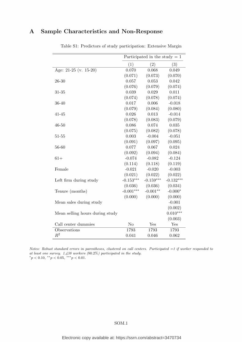
A Sample Characteristics and Non-Response

Table S1: Predictors of study participation: Extensive Margin

Participated in the study = 1

(1) (2) (3)

Age: 21-25 (v. 15-20) 0.070 0.068 0.049(0.071) (0.073) (0.070)

26-30 0.057 0.053 0.042(0.076) (0.079) (0.074)

31-35 0.039 0.029 0.011(0.074) (0.078) (0.074)

36-40 0.017 0.006 -0.018(0.079) (0.084) (0.080)

41-45 0.026 0.013 -0.014(0.078) (0.083) (0.079)

46-50 0.086 0.074 0.035(0.075) (0.082) (0.078)

51-55 0.003 -0.004 -0.051(0.091) (0.097) (0.095)

56-60 0.077 0.067 0.024(0.092) (0.094) (0.084)

61+ -0.074 -0.082 -0.124(0.114) (0.118) (0.119)

Female -0.021 -0.020 -0.003(0.021) (0.022) (0.022)

Left firm during study -0.153∗∗∗ -0.159∗∗∗ -0.132∗∗∗

(0.036) (0.036) (0.034)Tenure (months) -0.001∗∗∗ -0.001∗∗ -0.000∗

(0.000) (0.000) (0.000)Mean sales during study -0.001

(0.002)Mean selling hours during study 0.010∗∗∗

(0.003)Call center dummies No Yes Yes

Observations 1793 1793 1793R2 0.041 0.046 0.062

Notes: Robust standard errors in parentheses, clustered on call centers. Participated =1 if worker responded toat least one survey. 1,438 workers (80.2%) participated in the study.∗p < 0.10, ∗∗p < 0.05, ∗∗∗p < 0.01.

SOM.1


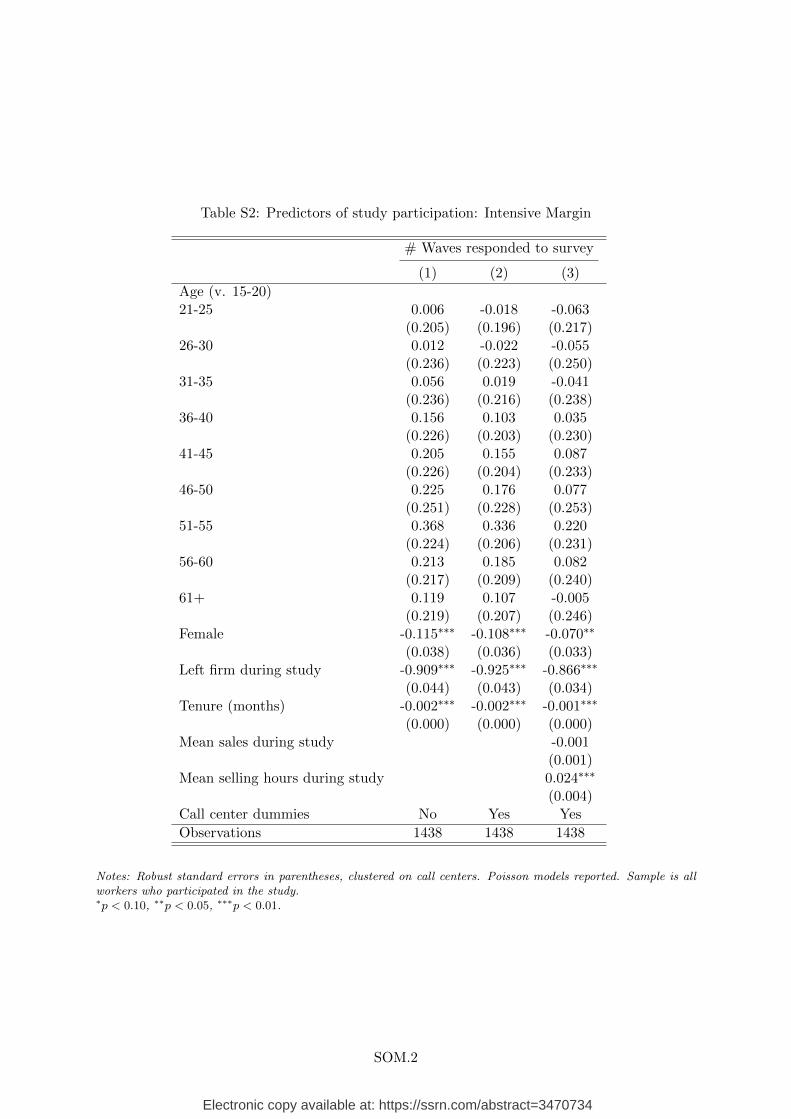
Table S2: Predictors of study participation: Intensive Margin

# Waves responded to survey

(1) (2) (3)

Age (v. 15-20)21-25 0.006 -0.018 -0.063

(0.205) (0.196) (0.217)26-30 0.012 -0.022 -0.055

(0.236) (0.223) (0.250)31-35 0.056 0.019 -0.041

(0.236) (0.216) (0.238)36-40 0.156 0.103 0.035

(0.226) (0.203) (0.230)41-45 0.205 0.155 0.087

(0.226) (0.204) (0.233)46-50 0.225 0.176 0.077

(0.251) (0.228) (0.253)51-55 0.368 0.336 0.220

(0.224) (0.206) (0.231)56-60 0.213 0.185 0.082

(0.217) (0.209) (0.240)61+ 0.119 0.107 -0.005

(0.219) (0.207) (0.246)Female -0.115∗∗∗ -0.108∗∗∗ -0.070∗∗

(0.038) (0.036) (0.033)Left firm during study -0.909∗∗∗ -0.925∗∗∗ -0.866∗∗∗

(0.044) (0.043) (0.034)Tenure (months) -0.002∗∗∗ -0.002∗∗∗ -0.001∗∗∗

(0.000) (0.000) (0.000)Mean sales during study -0.001

(0.001)Mean selling hours during study 0.024∗∗∗

(0.004)Call center dummies No Yes Yes

Observations 1438 1438 1438

Notes: Robust standard errors in parentheses, clustered on call centers. Poisson models reported. Sample is allworkers who participated in the study.∗p < 0.10, ∗∗p < 0.05, ∗∗∗p < 0.01.

SOM.2


Table S3: Predictors of attrition/non-response

Responded to Survey = 1

(1) (2) (3) (4)

Sales -0.000 -0.000 -0.000 -0.000(0.000) (0.000) (0.000) (0.000)

Selling time 0.012∗∗∗ 0.012∗∗∗ 0.012∗∗∗ 0.012∗∗∗

(0.001) (0.001) (0.001) (0.001)Bad weather index 0.001 0.001

(0.002) (0.002)Team happiness (excl worker) -0.001 -0.001

(0.003) (0.003)

Observations 33725 33725 33725 33725R2 0.436 0.436 0.436 0.436

Notes: Robust standard errors in parentheses, clustered on individuals. Linear models reported. Unit of observa-tion is worker*week. Individual and week fixed effects in all models.∗p < 0.10, ∗∗p < 0.05, ∗∗∗p < 0.01.

SOM.3


B Measurement Error: IV Estimates using Peer Happiness

Table S4: Happiness and Productivity: IV estimates using peers’ happiness

Sales(Poisson)

Happiness(OLS)

Sales(Poisson)


Happiness (1-5) 0.3143∗∗∗

(0.0920)Team Happiness 0.0111∗∗∗ 0.0362∗∗∗

(0.0034) (0.0105)


Notes: Columns (1) and (3) are Poisson-FE models. Column (2) reports an OLS-FE regression. Column (3)reports the second stage of a Poisson-FE control function model. Robust standard errors in parentheses, clusteredon individuals in models (1) and (2). Bootstrapped standard errors reported for model (3). All models includeindividual and week fixed effects, work schedule controls, and day of response to survey. ∗p < 0.10, ∗∗p < 0.05,∗∗∗p < 0.01.

SOM.4


C Customer Satisfaction

Table S5: Happiness and Customer Satisfaction

Customer Satisfaction (z-score)

(1) (2) (3) (4)OLS-FE OLS-FE 2SLS 2SLS

Happiness (1-5) 0.0168∗ 0.0137 -0.3767 -0.4015(0.0094) (0.0094) (0.3185) (0.3329)

# Sales 0.0034∗∗∗ 0.0081∗∗

(0.0013) (0.0039)

Observations 10,062 10,062 10,062 10,062Employees 1,082 1,082 1,082 1,082R2 0.173 0.174 -0.173 -0.190

Notes: Columns (1) and (2) are OLS-FE models. Column (3) and (4) report Second-stage 2SLS regressions.Robust standard errors in parentheses, clustered on individuals. Weekly customer satisfaction is z-scored.All models include individual and week fixed effects, work schedule controls, and day of response to survey.∗p < 0.10, ∗∗p < 0.05, ∗∗∗p < 0.01.

SOM.5


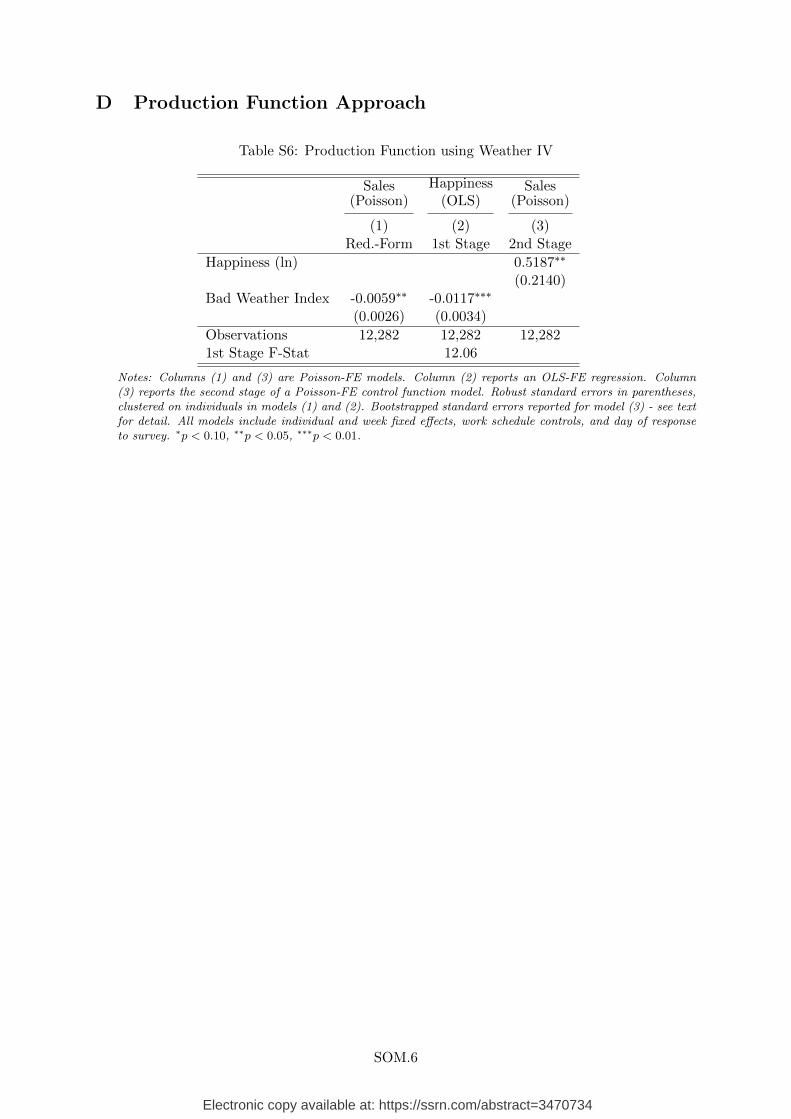
D Production Function Approach

Table S6: Production Function using Weather IV

Sales(Poisson)

Happiness(OLS)

Sales(Poisson)


Happiness (ln) 0.5187∗∗


(0.0026) (0.0034)


Notes: Columns (1) and (3) are Poisson-FE models. Column (2) reports an OLS-FE regression. Column(3) reports the second stage of a Poisson-FE control function model. Robust standard errors in parentheses,clustered on individuals in models (1) and (2). Bootstrapped standard errors reported for model (3) - see textfor detail. All models include individual and week fixed effects, work schedule controls, and day of responseto survey. ∗p < 0.10, ∗∗p < 0.05, ∗∗∗p < 0.01.

SOM.6


Table S7: Production Function: Happiness and Labor Productivity

Adherence(Met Target=1)

Minutes Per Call(Log)

Conversion Rate(Log)

(1) (2) (3) (4) (5) (6)

Happiness (ln) 0.5590∗∗ 0.5610∗∗ -0.3894∗∗∗ -0.4069∗∗ 1.1283∗∗∗ 1.3529∗∗∗

(0.2747) (0.2768) (0.1500) (0.1707) (0.4137) (0.4391)Sales (ln) 0.0373∗∗

(0.0185)Minutes per call (ln) 0.6776∗∗∗

(0.1006)

Observations 12,175 12,175 12,100 11,979 11,720 11,720

Notes: Second-stage 2SLS models reported, using adverse weather index as an IV for (log) happiness. Robuststandard errors in parentheses, clustered on individuals. All models include individual and week fixed effects,and controls for log working hours, internal training time, and day of response to survey. ∗p < 0.10, ∗∗p <0.05, ∗∗∗p < 0.01.

Table S8: Production Function: Happiness and Labor Supply

Attendance Sick Leave Overtime Paid Vacation Paid Breaks Unpaid Breaks

(100% =1 ) (Any = 1) (Any = 1) (Any = 1) (Minutes) (Minutes)

Happiness (ln) -0.1444 0.3513∗ -0.1827 -0.2926 -10.0697 -41.4512(0.3347) (0.1850) (0.1563) (0.2733) (6.4880) (44.4289)

Observations 12,285 12,285 12,288 12,288 12,288 12,288

Notes: Second-stage 2SLS models reported, using adverse weather index as an IV for (log) happiness. Robuststandard errors in parentheses, clustered on individuals. All models include include individual and week fixedeffects and dummies for day of response to survey. ∗p < 0.10, ∗∗p < 0.05, ∗∗∗p < 0.01.

SOM.7


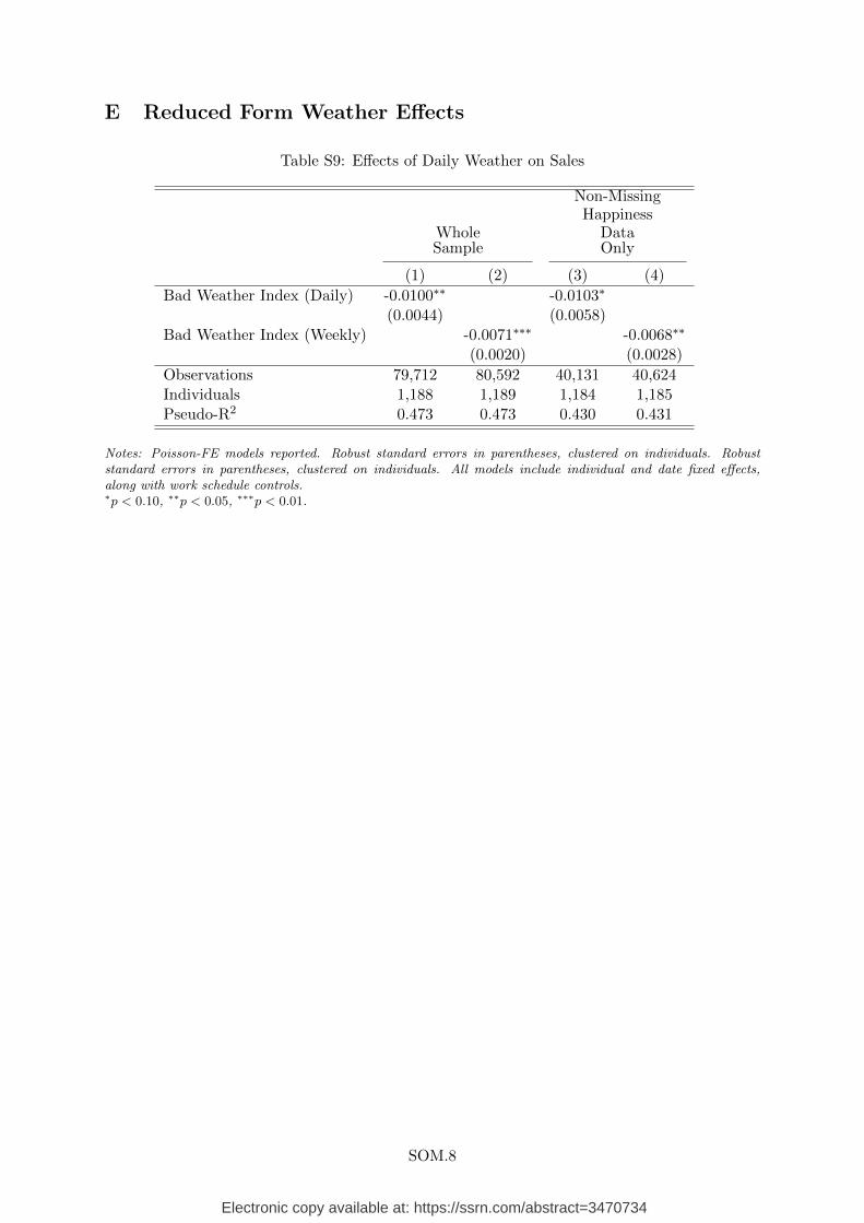
E Reduced Form Weather Effects

Table S9: Effects of Daily Weather on Sales

WholeSample

Non-MissingHappiness

DataOnly

(1) (2) (3) (4)

Bad Weather Index (Daily) -0.0100∗∗ -0.0103∗

(0.0044) (0.0058)Bad Weather Index (Weekly) -0.0071∗∗∗ -0.0068∗∗

(0.0020) (0.0028)

Observations 79,712 80,592 40,131 40,624Individuals 1,188 1,189 1,184 1,185Pseudo-R2 0.473 0.473 0.430 0.431

Notes: Poisson-FE models reported. Robust standard errors in parentheses, clustered on individuals. Robuststandard errors in parentheses, clustered on individuals. All models include individual and date fixed effects,along with work schedule controls.∗p < 0.10, ∗∗p < 0.05, ∗∗∗p < 0.01.

SOM.8


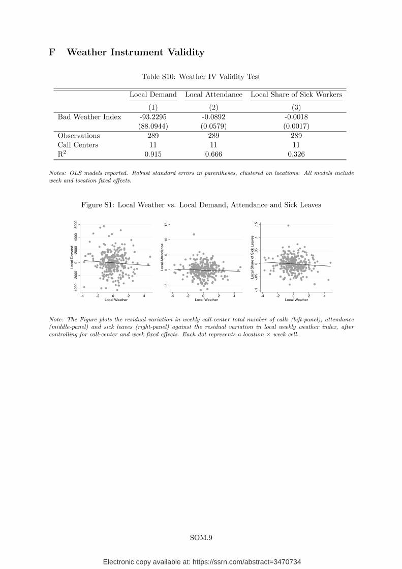
F Weather Instrument Validity

Table S10: Weather IV Validity Test

Local Demand Local Attendance Local Share of Sick Workers

(1) (2) (3)

Bad Weather Index -93.2295 -0.0892 -0.0018(88.0944) (0.0579) (0.0017)

Observations 289 289 289Call Centers 11 11 11R2 0.915 0.666 0.326

Notes: OLS models reported. Robust standard errors in parentheses, clustered on locations. All models includeweek and location fixed effects.

Figure S1: Local Weather vs. Local Demand, Attendance and Sick Leaves

-400

0-2

000

020

0040

0060

00Lo

cal D

eman

d

-4 -2 0 2 4Local Weather

-50

510

15Lo

cal A

ttend

ance


-.1-.0

50

.05

.1.1

5Lo

cal S

hare

of S

ick

Leav

es


Note: The Figure plots the residual variation in weekly call-center total number of calls (left-panel), attendance(middle-panel) and sick leaves (right-panel) against the residual variation in local weekly weather index, aftercontrolling for call-center and week fixed effects. Each dot represents a location × week cell.

SOM.9


Table S11: Bad Weather Index and Happiness: Heterogeneous Treatment Effects

Happiness

(1) (2) (3) (4) (5) (6)

Bad Weather Index -0.0247∗∗∗ -0.0175∗ -0.0128 -0.0262∗∗∗ -0.0294∗∗∗ -0.0288∗∗∗

(0.0076) (0.0093) (0.0236) (0.0092) (0.0097) (0.0109)Bad Weather Interaction:x Female Worker -0.0181

(0.0143)x Worker’s Age -0.0003

(0.0006)x Worker’s Tenure (Years) 0.0003

(0.0008)x Worker Avg Happiness > Median 0.0097

(0.0136)x # Sales 0.0002

(0.0003)

Observations 12,282 12,282 12,282 12,282 12,282 12,282Individuals 1,157 1,157 1,157 1,157 1,157 1,157R2 0.534 0.534 0.534 0.534 0.534 0.538

Notes: OLS-FE models reported. Robust standard errors in parentheses, clustered on individuals. All modelsinclude individual and week fixed effects, work schedule controls, and day of response to survey. Column (6) alsocontrols for weekly sales as it varies within workers.∗p < 0.10, ∗∗p < 0.05, ∗∗∗p < 0.01.

SOM.10


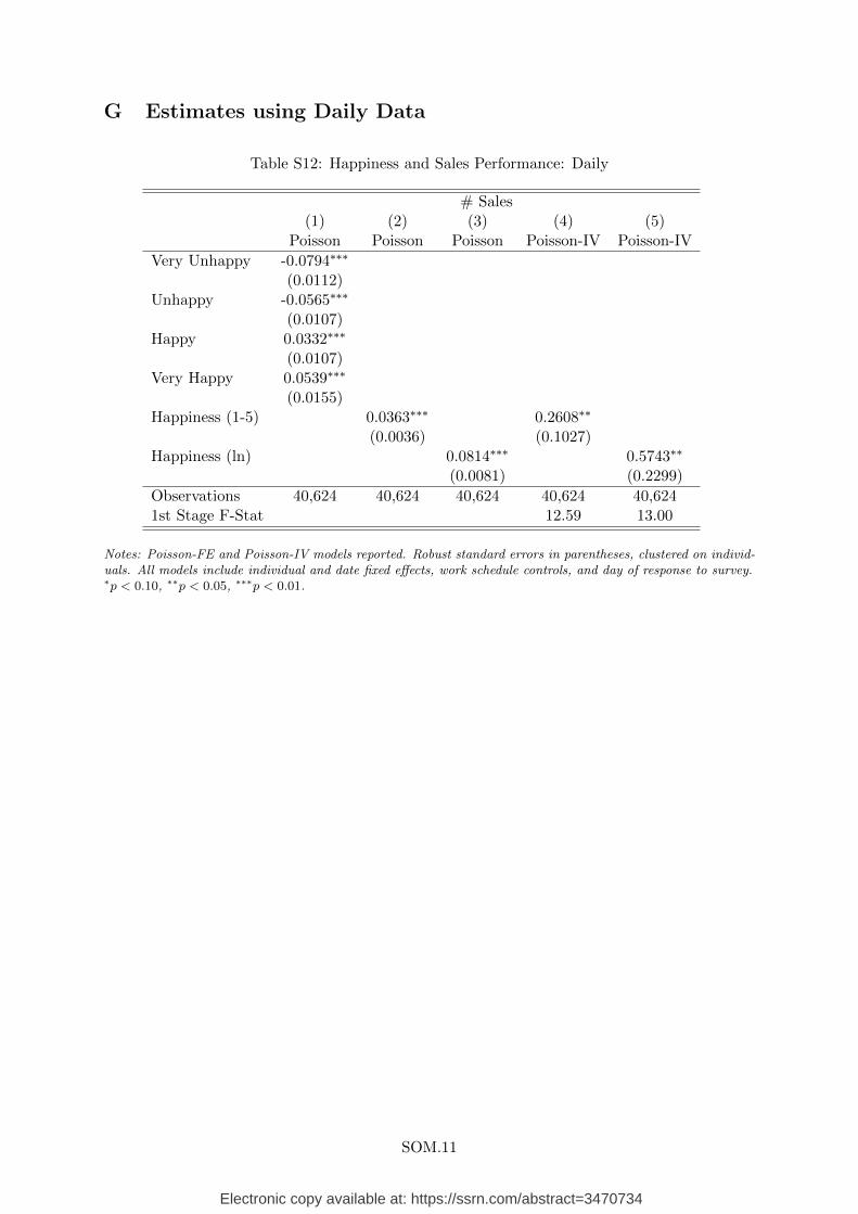
G Estimates using Daily Data

Table S12: Happiness and Sales Performance: Daily

# Sales(1) (2) (3) (4) (5)

Poisson Poisson Poisson Poisson-IV Poisson-IV

Very Unhappy -0.0794∗∗∗

(0.0112)Unhappy -0.0565∗∗∗

(0.0107)Happy 0.0332∗∗∗

(0.0107)Very Happy 0.0539∗∗∗

(0.0155)Happiness (1-5) 0.0363∗∗∗ 0.2608∗∗

(0.0036) (0.1027)Happiness (ln) 0.0814∗∗∗ 0.5743∗∗

(0.0081) (0.2299)

Observations 40,624 40,624 40,624 40,624 40,6241st Stage F-Stat 12.59 13.00

Notes: Poisson-FE and Poisson-IV models reported. Robust standard errors in parentheses, clustered on individ-uals. All models include individual and date fixed effects, work schedule controls, and day of response to survey.∗p < 0.10, ∗∗p < 0.05, ∗∗∗p < 0.01.

SOM.11


H Linear Estimates

Table S13: Linear Estimates

Ln(Sales) Ln(Sales+1)

(1) (2) (3) (4) (5) (6)OLS-FE OLS-FE 2SLS OLS-FE OLS-FE 2SLS

Happiness (vs. neutral)Very Unhappy -0.0715∗∗∗ -0.0687∗∗∗

(0.0131) (0.0123)Unhappy -0.0479∗∗∗ -0.0405∗∗∗

(0.0134) (0.0127)Happy 0.0367∗∗∗ 0.0247∗∗

(0.0131) (0.0126)Very Happy 0.0674∗∗∗ 0.0512∗∗∗

(0.0175) (0.0179)Happiness (Continuous)Happiness (1-5) 0.0362∗∗∗ 0.6364∗∗∗ 0.0310∗∗∗ 0.6092∗∗∗

(0.0041) (0.2266) (0.0041) (0.2277)

Observations 12,292 12,292 12,025 12,555 12,555 12,2881st Stage F-Stat 10.51 10.30

Notes: OLS-FE and Second-stage 2SLS models reported. Robust standard errors in parentheses, clustered onindividuals. All models include individual and week fixed effects, work schedule controls, and day of response tosurvey.∗p < 0.10, ∗∗p < 0.05, ∗∗∗p < 0.01.

SOM.12


I Heterogeneity by Demographics

Table S14: Happiness and Sales Performance: Heterogeneity

# Sales

(1) (2) (3) (4) (5)

Happiness (1-5) 0.0349∗∗∗ 0.0316∗∗∗ 0.0481∗∗∗ 0.0372∗∗∗ 0.0322∗∗∗

(0.0034) (0.0042) (0.0116) (0.0041) (0.0050)Happiness (1-5) × Female Worker 0.0096

(0.0068)Happiness (1-5) × Worker’s Age -0.0004

(0.0004)Happiness (1-5) × Tenure (Years) -0.0006

(0.0005)Happiness (1-5) × Worker Avg Happiness > Median 0.0050

(0.0066)

Observations 12,549 12,549 12,549 12,549 12,549Individuals 1,161 1,161 1,161 1,161 1,161Pseudo-R2 0.626 0.626 0.626 0.626 0.626

Notes: Poisson-FE models reported. Robust standard errors in parentheses, clustered on individuals. All modelsinclude individual and week fixed effects, work schedule controls, and day of response to survey.∗p < 0.10, ∗∗p < 0.05, ∗∗∗p < 0.01.

SOM.13


J Mechanisms: Robustness

Table S15: Happiness and Performance-Related Pay

# Sales

(1) (2) (3) (4)

Happiness (1-5) 0.0349∗∗∗ 0.0324∗∗∗

(0.0034) (0.0072)Happiness × High Performance Pay 0.0031


(0.0026) (0.0048)Bad Weather Index × High Performance Pay 0.0148∗∗∗

(0.0051)

Observations 12549 12549 12282 12282Individuals 1,161 1,161 1,157 1,157Pseudo-R2 0.626 0.626 0.617 0.617

Notes: Poisson-FE models reported. Robust standard errors in parentheses, clustered on individuals. Allmodels include individual and week fixed effects, work schedule controls, and day of response to survey.∗p < 0.10, ∗∗p < 0.05, ∗∗∗p < 0.01.

Table S16: Happiness and Multi-Tasking

# Sales

(1) (2)

Happiness (1-5) 0.0378∗∗∗

(0.0039)Happiness (1-5) × Other Tasks (% Working Hours) -0.0004

(0.0004)Bad Weather Index -0.0080∗∗∗

(0.0030)Bad Weather Index × Other Tasks (% Working Hours) 0.0004

(0.0003)Other Tasks (% Working Hours) -0.0010 -0.0039∗∗∗

(0.0013) (0.0011)

Observations 12,521 12,255Individuals 1,159 1,155Pseudo-R2 0.625 0.616


SOM.14


Table S17: Happiness and Emotional Skills

# Sales

(1) (2)

Happiness (1-5) 0.0352∗∗∗

(0.0033)Happiness (1-5) × Weekly Customer Satisfaction -0.0045∗

(0.0027)Bad Weather Index -0.0038

(0.0026)Bad Weather Index × Weekly Customer Satisfaction 0.0111∗∗∗

(0.0019)

Observations 12,549 12,282Individuals 1,161 1,157Pseudo-R2 0.626 0.618


SOM.15


does employee happiness have an impact on productivity?

Documents