Does complex always mean powerful? A comparison of eight methods for interpolation of climatic data in Mediterranean areaMaurizio Marchi1,*, Ugo Chiavetta1, Cristiano Castaldi1, Fulvio Ducci1

Ital

ian

Jour

nal o

f Agr

omet

eoro

logy

- 1/

2017

Riv

ista

Ita

liana

di A

grom

eteo

rolo

gia

-1/2

017

59

Abstract: Biodiversity will probably be threatened by climate change effects and the Mediterranean area is a well know hotspot of genetic diversity. Climatic data are a very important source of information for those studies and the aim of this work was to study and compare eight methods for spatial interpolation of climatic data and indices including parametric and non-parametric methods, deterministic, regressive and geostatistical. The Root Mean Square Error (RMSE), relative RMSE (rRMSE) and relative BIAS (rBIAS) were calculated to assess algorithm’s performances in a Mediterranean region. None of the eight methods performed much better than others with a very complex physiographic environment. The range of errors was very high and rRMSE varied from 3.8% to 295%. Anyway, even in case of low differences among methods and despite the necessity of the assumption of normality of data, the interpolation at local scale with parametric and geostatistical methods (e.g. kriging or cokriging) should be preferred to globally-interpolated climatic data due to the possibility to obtain the distribution of prediction’s error.Keywords: Spatial interpolation; Abruzzo; climatic data, Mediterranean area; kriging.

Riassunto: All’interno dell’area Mediterranea, ben conosciuta per via del suo alto tasso di ricchezza genetica, l’Italia centro-meridionale è una zona molto importante per via del suo clima e delle sue caratteristiche filogenetiche. Per studiare questo tipo di interazioni i dati climatici rappresentano una rilevante fonte di informazione e obbiettivo di questo studio è stato quello di valutare e comparare otto metodi per l’interpolazione spaziale di variabili ed indici climatici includendo metodi parametrici e non metodi deterministici, regressivi e geostatistici. La valutazione della qualità di interpolazione è stata effettuata attraverso tre stimatori: il Root Mean Square Error assoluto (RMSE) e percentuale (rRMSE) ed il relative BIAS (rBIAS). L’analisi ha evidenziato l’assenza di un modello nettamente migliore con un errore medio relativo variabile tra il 3.8% ed il 295% a causa di una mancanza di correlazioni statistiche tra variabili dipendenti e predittori. Tuttavia l’utilizzo di dati locali con metodi geostatistici è risultata essere comunque la scelta migliore grazie alla potenzialità di fornire la distribuzione spaziale dell’errore di interpolazione.Parole chiave: Interpolazione spaziale; Abruzzo; dati climatici; Zona Mediterranea; kriging.

* Corresponding author’s e-mail: maurizio.marchi@crea.gov .it1 Consiglio per la ricerca in agricoltura e l’analisi dell’economia agraria - Forestry Research Centre, Arezzo, Italy.Received 19 December 2015, accepted 17 August 2016

DOI:10.19199/2017.1.2038-5625.059

IntRoductIonIn the last twenty years, since Kyoto protocol, climatic data gained more and more attention due to increasing interest on climate change and its possible effects on organisms (Parmesan, 1996; Martinez-Meyer, 2005; Mátýas et al., 2009; Schueler et al., 2014). Many studies are focused on possible impacts of Global Change on forest ecosystems and animals with the aim to forecast future developments (Pearson and Dawson, 2003; Cheaib et al., 2012; Provan and Maggs, 2012; Vacchiano and Motta, 2014, Marchi et al., 2016). Minimum requirements of these studies are long-term climate baseline data, future predictions and, in some cases, even information about past climate variability. Anyway, they are usually not easily accessible at the appropriate resolution for a comprehensive set of biologically relevant climate variables. At the same

time, data always need a quality check to ensure the absence of missing periods and storage errors. Many statistical techniques has been investigated to complete or to fill gaps in climatic data series (Paulhus and Kohler, 1952; Xia et al., 1999; Eischeid et al., 2000; Schneider, 2001; Ramosand Calzado et al., 2008; Wilks, 2011). The correct selection of one method depends on the data use and the purpose of the study. In addition, a key role is played by the representativeness of the meteorological network (Wong et al., 2004; Bhowmik and Costa, 2014) often masked by a regular spatial coverage but which does not cover all the physiograpic features of a given spatial extent (e.g. higher elevations).Due to spreading of web knowledge and data storage, many datasets are freely available in literature (temperature, rainfall, climatic indices) e.g. at national (Wang et al., 2012) or global scale (Hijmans et al., 2005) but often not adequate for local studies and in very variable environments. When a more detailed information is required statistical downscaling (Wang et al., 2012; Jones and Thornton, 2013) and interpolation

CIANO AGRO 1-17.indb 59 04/04/17 16.42

Ital

ian

Jour

nal o

f Agr

omet

eoro

logy

- 1/

2017

Riv

ista

Ita

liana

di A

grom

eteo

rolo

gia

-1/2

017

60

autocorrelation) but a more complex variogram which uses cross-covariance functions. Consequently, it is more time-consuming and demonstrated to be very powerful when secondary information is abundant and easy to sample across the study area, e.g. radar data (Schuurmans et al., 2007).Among the non parametric methods, the inverse distance weighted (IDW), K-Nearest Neighbour (k-NN) and spline functions are the most common methods. IDW is a deterministic, geostatistic but non-parametric method for local interpolation. Values at unknown points are calculated as the weighted average of the values available at the known points and weights are calculated in relation to the spatial distances from the point to be interpolated and the nearest known points. Typical problems of this method are that maximum and minimum values are always known points of the dataset and distance between points do not consider differences in elevations, aspects, etc. Thus, for instance, with IDW algorithm, temperatures on the top of relieves are very difficult to estimate and to avoid spatial drifts and when correlation between data to be interpolate and a co-variable is high enough, a detrended-IDW (D-IDW) can be used (Kurtzman and Kadmon, 1999; Attorre et al., 2008). K-Nearest Neighbour (k-NN) algorithm (Cover and Hart, 1967) instead is generally used for classification of objects. It is based on multidimensional proximity between objects and, similar to IDW, the unknown object is classified by a majority vote of its neighbours. The main difference between IDW and k-NN is the calculation of proximity between observations, evaluated in k-NN not in a geographical sense but in a new multidimensional space. New coordinates of this space are two or more variables measured over the whole study area. K-NN have been widely used in Forestry to estimate forest variables such as volume or cover type (Franco-Lopez et al., 2001; Mäkelä and Pekkarinen, 2004; Chiavetta and Chirici, 2008; Lasserre et al., 2011; Chirici et al., 2012) but, in some cases, also for predicting climatic scenarios (Yates, 2003; Sharif et al., 2007). Anyway, even if the application of the method in meteorology is limited, in some cases it may be successful for dense measurement networks. Finally splines polynomial functions which interpolates data dividing the dataset in subregions. It is a method that has been widely used to interpolate climatic factors due to its speed and usability (Hofierka et al., 2002; Hijmans et al., 2005; Yilmaz and Tolunay, 2012).In the end, each method has its pros and cons, mainly connected to nature of data and study cases. Most of the studies in literature used comparative methods, aware that the quality of spatial interpolation

of climatic data obtained by local monitoring network (Attorre et al., 2007; Chai, 2011) are the only feasible approaches. Downscaling methods are generally based on regressions (singular, polynomial or splines) and are mainly used to improve prediction at finer resolution (Pellatt et al., 2012, Marchi et al., 2015) whereas interpolation methods are used very frequently in climatology and applied studies.To interpolate climatic data, many parametric and non-parametric methods are available in literature. Main methods enclose different algorithms of distance weighting (Kurtzman and Kadmon, 1999), single and multiple linear regressions (Blasi et al., 2007; Hofstra et al., 2008; Brunetti et al., 2014), nearest neighbour algorithms (Kao and Hung, 2004), spline functions (Hofierka et al., 2002) and geostatistical methods like kriging and co-kriging in their various variants (Van Houwelingen and Le Cressie, 1990; Attorre et al., 2008; Li and Heap, 2008; Brunetti et al., 2014). All these methods can be grouped into two main big families: parametric and non-parametric. In case of climatic data and especially for temperature, elevation is often the main driving factor and this assumption is used for interpolation or Downscaling (Hijmans et al., 2005; Blasi et al., 2007; Wang et al., 2012). For the whole Italian territory, Blasi and others (2007), for example, used a weighted regression method with elevation to interpolate temperature data, weighting the nearest meteorological stations included into a 20 km radius for each pixel at a geometrical resolution of 250 m. However the most famous and used parametric interpolation methods is krining (Krige, 1951) developed by D. G. Krige for minereary purposes introducing moving averages and geostatistical processes to avoid systematic errors. This method is also known as the “Gaussian process” and is believed to be the Best Linear Unbiased Method (Li and Heap, 2008). The variogram (or semivariogram) analysis is the core of computation as an evaluation of spatial correlation among observational points as function of distance between points and direction of variance. Parameters of the (semi)variogram model are: model (most used are linear, exponential, circular, spherical and Gaussian), range, sill and nugget. Range is the distance value at which the model begins to become flat (end of autocorrelation), sill is the value of (semi)variance at the range value and nugget is the value of (semi)variance at zero distance. Many different types of kriging and methods are possible, which can work differently with the same dataset. Among them cokriging can be considered as an extension of kriging with the same assumption (normalized data, random distribution of points, analysis of

CIANO AGRO 1-17.indb 60 04/04/17 16.42

Ital

ian

Jour

nal o

f Agr

omet

eoro

logy

- 1/

2017

Riv

ista

Ita

liana

di A

grom

eteo

rolo

gia

-1/2

017

61

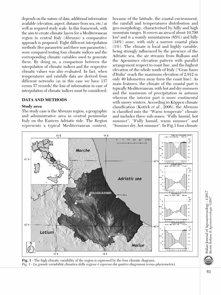
because of the latitude, the coastal environment, the rainfall and temperatures distribution and geo-morphology, characterised by hilly and high mountain ranges. It covers an area of about 10,700 km2 and is a mainly mountainous (65%) and hilly (34%) zone, with only a narrow coastal plain (1%). The climate is local and highly variable, being strongly in� uenced by the presence of the Adriatic sea, the air streams from Balkans and the Apennines elevation pattern with parallel arrangement respect to coast line, and the highest elevation of the whole south of Italy (“Gran Sasso d’Italia” reach the maximum elevation of 2,912 m only 40 kilometres away form the coast line). As main features, the climate of the coastal part is typically Mediterranean, with hot and dry summers and the maximum of precipitation in autumn whereas the interior part is more continental with snowy winters. According to Köppen climate classi� cation (Kottek et al., 2006), the Abruzzo is classi� ed into the “Warm temperate” climate and includes three sub-zones: “Fully humid, hot summer”, “Fully humid, warm summer” and “Summer dry, hot summer”. In Fig. 1 four climate

depends on the nature of data, additional information available (elevation, aspect, distance from sea, etc.) as well as required study scale. In this framework, with the aim to create climatic layers for a Mediterranean region in central Italy (Abruzzo) a comparative approach is proposed. Eight different interpolation methods (� ve parametric and three non parametric), were compared testing four climatic indices and the corresponding climatic variables used to generate them. By doing so, a comparison between the interpolation of climatic indices and the respective climatic values was also evaluated. In fact, when temperatures and rainfalls data are derived from different networks (as in this case we have 137 versus 57 records) the loss of information in case of interpolation of climatic indices must be considered.

DATA AND METHODS

Study areaThe study case is the Abruzzo region, a geographic and administrative area in central peninsular Italy on the Eastern Adriatic side. The Region represents a typical Mediterranean context,

Fig. 1 - The high climatic variability of the region is expressed by the four climatic diagrams.Fig. 1 - La grande variabilità climatica della regione è espressa dai quattro diagrammi termo-pluviometrici.

59-72 marchi_CORTO.indd 61 11/04/17 14.58

Ital

ian

Jour

nal o

f Agr

omet

eoro

logy

- 1/

2017

Riv

ista

Ita

liana

di A

grom

eteo

rolo

gia

-1/2

017

Those indices were:

1) De Martonne (1927) Aridity index:

where:MAP = Mean Annual PrecipitationDMP = Driest month Mean PrecipitationMAT = Mean Annual TemperatureDMT = Driest month Mean Temperature

2) Emberger (1930) Pluviotermic quotient:

where:MAP = Mean Annual PrecipitationHMTx = Hottest month Maximum TemperatureCMTm = Coldest month Minimum Temperature

62

diagrams are provided to give an idea of the high climatic variability of the region.

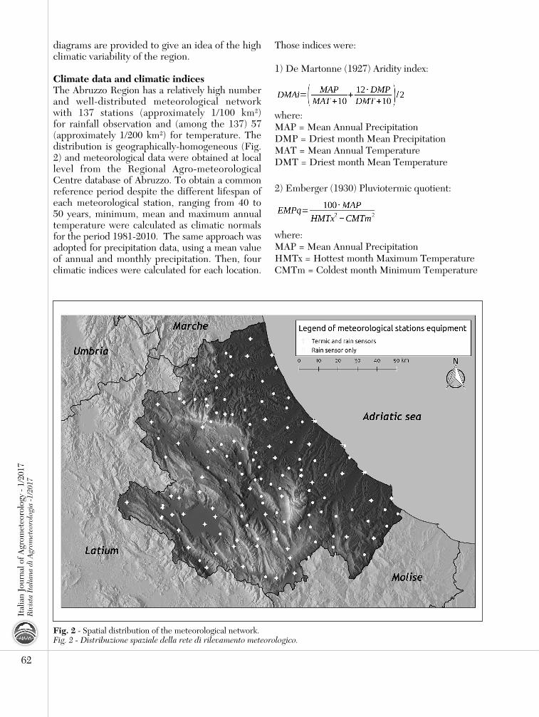
climate data and climatic indicesThe Abruzzo Region has a relatively high number and well-distributed meteorological network with 137 stations (approximately 1/100 km2) for rainfall observation and (among the 137) 57 (approximately 1/200 km2) for temperature. The distribution is geographically-homogeneous (Fig. 2) and meteorological data were obtained at local level from the Regional Agro-meteorological Centre database of Abruzzo. To obtain a common reference period despite the different lifespan of each meteorological station, ranging from 40 to 50 years, minimum, mean and maximum annual temperature were calculated as climatic normals for the period 1981-2010. The same approach was adopted for precipitation data, using a mean value of annual and monthly precipitation. Then, four climatic indices were calculated for each location.

Fig. 2 - Spatial distribution of the meteorological network. Fig. 2 - Distribuzione spaziale della rete di rilevamento meteorologico.

CIANO AGRO 1-17.indb 62 04/04/17 16.42

3) Rivas Martinez (1996) Continentality index:

where:HMT = Hottest Month mean TemperatureCMT = Coldest Month mean Temperature

4) Rivas Martinez (1996) Thermal index:

where:MAT = Mean Annual TemperatureCMTx = Coldest month Maximum TemperatureCMTm = Coldest month Minimum Temperature

Climatic data were geo-referenced in WGS84 UTM 33 North reference system (EPSG 32633) and to perform data interpolation, the most

commonly-used independent physiographic parameters were obtained form the DEM with 10 meters of spatial resolution. Those independent variables were: latitude (LAT), longitude (LONG) Elevation (ELEV), Aspect (ASP), Distance from sea (DSEA). Global Solar Radiation (GSR) was added to this database and calculated with the r.sun module of GRASS GIS software (GRASS Development Team, 2015). All the acronyms are reported in table (Tab. 1).

tested algorithmsAfter a literature review, eight algorithms were selected. Inverse Distance Weighted (IDW) and k-nearest neighbor (K-NN) were selected as fast and easy deterministic method. Concerning splines, Regularized Spline with Tension (RST) was considered as example and as the main method

63

Ital

ian

Jour

nal o

f Agr

omet

eoro

logy

- 1/

2017

Riv

ista

Ita

liana

di A

grom

eteo

rolo

gia

-1/2

017

Name Acronym

Interpolation methods

Linear Regression REGK Nearest Neighbors K-NN

Regularized Spline with Tension RSTInverse Distance Weighted IDW

Ordinary Kriging OKUniversal Kriging UK

Regression Kriging RKOrdinary Cokriging OCK

Physiographic parameters

Latitude LATLongitude LONGElevation ELEV

Aspect ASPDistance from sea DSEA

Global Solar Radiation GSR

climatic variables

Mean Annual Precipitation MAPDriest Month mean Precipitation DMP

Mean Annual Temperature MATDriest Month mean Temperature DMT

Hottest Month mean Temperature HMTHottest Month maximum Temperature HMTx

Coldest Month mean Temperature CMTColdest Month minimum Temperature CMTmColdest Month maximum Temperature CMTx

De Martonne Aridity index DMAiEmberger Pluviotermic quotient EMPq

Rivas Martinez Continentality index RMCiRivas Martinez Termic index RMTi

tab. 1 - Table of Acronyms.Tab. 1 - Tabella degli acronimi.

CIANO AGRO 1-17.indb 63 04/04/17 16.42

Ital

ian

Jour

nal o

f Agr

omet

eoro

logy

- 1/

2017

Riv

ista

Ita

liana

di A

grom

eteo

rolo

gia

-1/2

017

64

of GRASS GIS software. Similar to splines, RST (Mitas and Mitasova, 1999) is a non-parametric interpolation method which belongs to numerical analysis and works dividing the interval of analysis in more sub-interval. Tension, smoothing, segmax (maximum number of points in the segment) and npmin (minimum number of points used for interpolation) are the main parameters to be set to modulate interpolation, generally through a cross validation procedure (typically a leave-one-out). High parameters force the surface shape (especially smoothing) so they also describe how far from the real values the surface will be.Among parametric methods Multivariate Linear Regression (REG) was used as an example of general ordinary least squares estimators while ordinary kriging (OK), universal kriging (UK), regression kriging (RK) and ordinary cokriging (OCK) were used as most powerful and well referenced parametric and statical ones. The main differences between those kriging’s variants can be found in the computational steps. While in OK the spatial variation of the variable is assumed to be statistically homogeneous in the whole area, with UK the spatial variation (and the mean) is driven by an external drift which is added to the Kriging model to improve the prediction. For this reason, UK is often alternatively called “Kriging with external Drift” and often used in climatology (Attorre et al., 2007). RK instead is a term that has been used to define many different types of procedures, from “Kriging after detrending” where the trend function and estimated detrended variables are modelled separately to a combination of a regressive model of the independent variable on auxiliary variables with ordinary kriging of regression residuals (Odeh et al., 1995). Anyway, considering that the first definition is mathematically equivalent to UK, RK must correspond to the second procedure. In the end, in this work, RK was used with residuals of MLR while the most correlated variable among ELEV, ASP and GSR we used as external drift for UK avoiding UK and RK to be equivalent.To compare models and to asses differences between them a cross-validation procedure was performed with a leave-one-out (LOO-CV) approach due to small number of observations. Root Mean Square Error (RMSE, eq. [1]) was used to assess algorithms’ accuracy as a simple and efficient parameter whereas relative BIAS (rBIAS, eq [2]) and relative RMSE (rRMSE, eq. [3]) were calculated to compare results with different scales (Celsius degrees for temperatures, millimetre for precipitation, pure numbers for indices). Finally

rRMSE was used to perform a non-parametric ANOVA through the Kruskal-Wallis rank sum test (Kruskal and Wallis, 1952) to search for meaningful differences among algorithms performances. Both rBIAS and rRMSE were expressed in percentage.

[1]

[2]

[3]

GRASS GIS 6.4.4 and R 3.2.2 (R CoreTeam, 2015) with added packages as gstat (Pebesma, 2004), raster (Hijmans, 2015) and rgdal (Bivand et al., 2015) were used for the statistical and geo-statistical analysis and interpolation. A summary of the tested algorithm is reported in Tab. 2.

ReSultS And dIScuSSIonAfter a dataset-screening the four climatic indices were calculated for each meteorological station where both temperature and precipitation were available (57 cases only). Normality of distribution was tested with the Kolmogorov-Smirnov normality test (Dallal and Wilkinson, 1986) and followed by a data transformation where necessary. A statistical analysis of meteorological data is compulsory to ensure the quality of data sets, to improve the accuracy of interpolation results (Chai, 2011). Not-normally distributed data, outliers and errors in data storage are the most common problems which influence negatively the statistical analysis and, consequently, the interpolation. In many cases data were not normally distributed (Tab. 3) and normalization was achieved using the logarithmic or the reciprocal transformation. In case of negative values of temperatures (e.g. CMTm), a transformation from Celsius to Kelvin degrees was made.A screening for detection of statistical trends in data structure was performed using a linear model. The regression form was calculated using a backward stepwise analysis based on the Akaike’s information criterion (AIC, Akaike, 1974) with the complete formula and no interaction (all predictors included) as starting model. The amount of explained variance

CIANO AGRO 1-17.indb 64 04/04/17 16.42

65

Ital

ian

Jour

nal o

f Agr

omet

eoro

logy

- 1/

2017

Riv

ista

Ita

liana

di A

grom

eteo

rolo

gia

-1/2

017

AlgorithmGeostatistical (x & y coord.)

Assumption of normality of the data

Variogram analysis

Variance of prediction

Software

REG No Yes(parametric method) No No R (stat)

K-NN No No(non-parametric method) No No R (kknn)

RST No No (non-parametric method) No No GRASS GIS

IDW Yes No(non-parametric method) Yes No R (gstat)

OK Yes Yes(parametric method) Yes Yes R (gstat)

UK Yes Yes(parametric method)

Yes(+external drift) Yes R (gstat)

RK Yes Yes(parametric method) Yes Yes R (gstat)

OCK Yes Yes(parametric method)

Yes(co-variogram) Yes R (gstat)

tab. 2 - Main features of the eight tested algorithms.Tab. 2 - Caratteristiche principali degli otto metodi testati.

Data D value p-valueMAP 0.0973 0.0029

Transformed MAP 0.0577 0.3210DMP 0.0917 0.0067

Transformed DMP 0.0604 0.2542MAT 0.1150 0.0582

Transformed MAT 0.1049 0.1228CMT 0.1365 0.0099

Transformed CMT 0.1100 0.0987CMTm 0.1436 0.0051

Transformed CMTm 0.1140 0.0654CMTx 0.1260 0.0247

Transformed CMTx 0.1131 0.0666DMT 0.1184 0.0453

Transformed DMT 0.1114 0.0755HMT 0.1012 0.1552HMTx 0.1160 0.0539MAP 0.0973 0.0029

Transformed MAP 0.0577 0.3210DMP 0.0917 0.0067

Transformed DMP 0.0604 0.2542DMAi 0.0959 0.2141EMPq 0.1220 0.0340

Transformed EMPq 0.0970 0.2012RMCi 0.1064 0.1115RMTi 0.1308 0.0164

Transformed RMTi 0.0959 0.2148tab. 3 - Kolmogorov-Smirnov normality test for considered variables(α 0.05).Tab. 3 - Test di normalità di Kolmogorov-Smirnov per le variabili considerate (α 0.05).

CIANO AGRO 1-17.indb 65 04/04/17 16.42

Ital

ian

Jour

nal o

f Agr

omet

eoro

logy

- 1/

2017

Riv

ista

Ita

liana

di A

grom

eteo

rolo

gia

-1/2

017

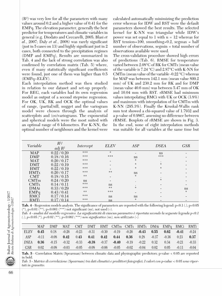
(R2) was very low for all the parameters with many values around 0.2 and a higher value of 0.41 for the EMPq. The elevation parameter, generally the best predictor for temperatures and climatic variables in general (e.g. Diodato and Ceccarelli, 2005; Blasi et al., 2007; Daly et al., 2008) was rarely significant (just in 5 cases on 13) and highly significant just in 2 cases, both connected to the precipitation regimes (DMP and EMPq), Results are summarized in Tab. 4 and the lack of strong correlation was also confirmed by correlation matrix (Tab. 5) where, even if many statistically significant coefficients were found, just one of them was higher than 0.5 (EMPq~ELEV).Each interpolation method was then studied in relation to our dataset and set-up properly. For REG, each variables had its own regression model as output of a second stepwise regression. For OK, UK, RK and OCK the optimal values of range, (partial)sill, nugget and the variogram model were chosen through the analysis of scatterplots and (co)variograms. The exponential and spherical models were the most suited with an optimal range of 6 kilometres. For K-NN, the optimal number of neighbours and the kernel were

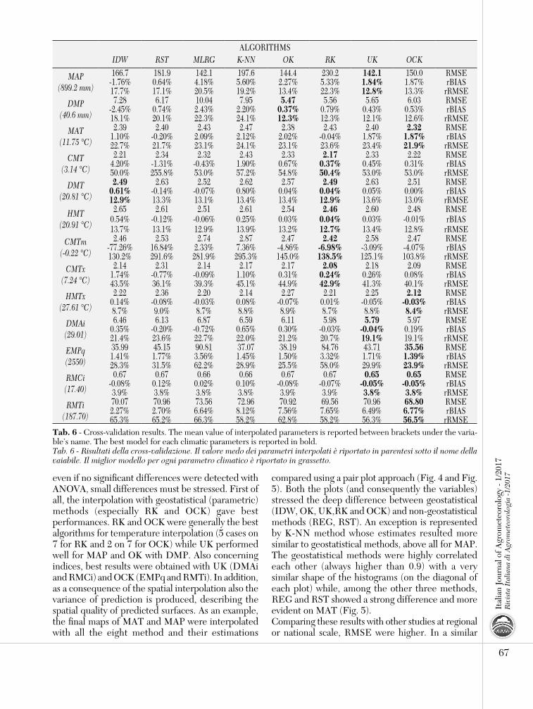
calculated automatically minimizing the prediction error whereas for IDW and RST were the default parameters showed the best results. The selected kernel for K-NN was triangular while IDW’s power was set equal to 1 with n = 12 whereas for RST tension=100, smoothing=0.2, segmax = half number of observations, segmin = total number of observations available were used.The cross-validation procedure showed high errors of predictions (Tab. 6). RMSE for temperature varied between 2.08°C of RK for CMTx (mean value of the variable is 7.24 °C) and 2.87°C with K-NN for CMTm (mean value of the variable -0.22 °C) whereas for MAP was between 142.1 mm (mean value 899.2 mm) of UK and 230.2 mm for RK and for DMP (mean value 40.6 mm) was between 5.47 mm of OK and 10.04 mm with RST. rRMSE had minimum values interpolating RMCi with UK or OCK (3.8%) and maximum with interpolation of for CMTm with K-NN (295.3%). Finally the Kruskal-Wallis rank sum test showed a chi-squared value of 1.7932 and a p-value of 0.9867, assessing no difference between rRMSE. Boxplots of rRMSE are shown in Fig. 3. In the end, none of eight interpolation methods was suitable for all variables at the same time but

66

VariableR2/

adj R2 Intercept ELEV ASP DSEA GSR

MAP 0.22 / 0.20 *** * - ns -DMP 0.18 / 0.16 *** *** ns *** -MAT 0.20 / 0.17 *** - * . -DMT 0.22 / 0.19 *** - * * -HMT 0.22 / 0.19 *** - * * -HMTx 0.20 / 0.17 *** ** ns - -CMT 0.18 / 0.15 ** - * . -

CMTm 0.24 / 0.20 ns - . * -CMTx 0.14 / 0.11 *** ns . - -DMAi 0.33 / 0.29 *** ** * - nsEMPq 0.43 / 0.41 ** *** - - *RMCi 0.17 / 0.14 *** ns ns - -RMTi 0.17 / 0.14 *** ns * - -

tab. 4 - Regression models analysis. The significance of parameters are reported with the following legend: p<0.1 (.), p<0.05 (*), p<0.01 (**), p<0.001 (***) not significant (ns), not used (-).Tab. 4 - analisi del modello regressivo. La significatività di ciascun parametro è riportata secondo la seguente legenda p<0.1 (.), p<0.05 (*), p<0.01 (**), p<0.001 (***) non significativo (ns), non utilizzato (-).

MAP DMP MAT CMT DMT HMT CMTm CMTx HMTx DMAi EMPq RMCi RMTiELEV 0.45 0.18 -0.26 -0.23 -0.31 -0.30 -0.19 -0.26 -0.43 0.55 0.62 -0.41 -0.24ASP -0.11 -0.08 0.42 0.43 0.41 0.42 0.44 0.36 0.28 -0.37 -0.36 0.23 0.37

DSEA 0.36 -0.15 -0.32 -0.33 -0.38 -0.37 -0.40 -0.19 -0.22 0.32 0.34 -0.21 -0.33GSR 0.02 -0.08 -0.03 -0.05 -0.08 -0.06 -0.05 -0.02 -0.04 0.02 0.05 -0.11 -0.04

tab. 5 - Correlation Matrix (Spearman) between climatic data and physiographic predictors; p-value < 0.05 are reported in bold.Tab. 5 - Matrice di correlazione (Spearman) tra dati climatici e predittori fisiografici; I valori con p-value < 0.05 sono ripor-tati in grassetto.

CIANO AGRO 1-17.indb 66 04/04/17 16.42

67

Ital

ian

Jour

nal o

f Agr

omet

eoro

logy

- 1/

2017

Riv

ista

Ita

liana

di A

grom

eteo

rolo

gia

-1/2

017compared using a pair plot approach (Fig. 4 and Fig.

5). Both the plots (and consequently the variables) stressed the deep difference between geostatistical (IDW, OK, UK,RK and OCK) and non-geostatistical methods (REG, RST). An exception is represented by K-NN method whose estimates resulted more similar to geostatistical methods, above all for MAP. The geostatistical methods were highly correlated each other (always higher than 0.9) with a very similar shape of the histograms (on the diagonal of each plot) while, among the other three methods, REG and RST showed a strong difference and more evident on MAT (Fig. 5).Comparing these results with other studies at regional or national scale, RMSE were higher. In a similar

even if no significant differences were detected with ANOVA, small differences must be stressed. First of all, the interpolation with geostatistical (parametric) methods (especially RK and OCK) gave best performances. RK and OCK were generally the best algorithms for temperature interpolation (5 cases on 7 for RK and 2 on 7 for OCK) while UK performed well for MAP and OK with DMP. Also concerning indices, best results were obtained with UK (DMAi and RMCi) and OCK (EMPq and RMTi). In addition, as a consequence of the spatial interpolation also the variance of prediction is produced, describing the spatial quality of predicted surfaces. As an example, the final maps of MAT and MAP were interpolated with all the eight method and their estimations

ALGORITHMSIDW RST MLRG K-NN OK RK UK OCK

MAP(899.2 mm)

166.7 181.9 142.1 197.6 144.4 230.2 142.1 150.0 RMSE-1.76% 0.64% 4.18% 5.60% 2.27% 5.33% 1.84% 1.87% rBIAS17.7% 17.1% 20.5% 19.2% 13.4% 22.3% 12.8% 13.3% rRMSE

DMP(40.6 mm)

7.28 6.17 10.04 7.95 5.47 5.56 5.65 6.03 RMSE-2.45% 0.74% 2.43% 2.20% 0.37% 0.79% 0.43% 0.53% rBIAS18.1% 20.1% 22.3% 24.1% 12.3% 12.3% 12.1% 12.6% rRMSE

MAT(11.75 °C)

2.39 2.40 2.43 2.47 2.38 2.43 2.40 2.32 RMSE1.10% -0.20% 2.09% 2.12% 2.02% -0.04% 1.87% 1.87% rBIAS22.7% 21.7% 23.1% 24.1% 23.1% 23.6% 23.4% 21.9% rRMSE

CMT(3.14 °C)

2.21 2.34 2.32 2.43 2.33 2.17 2.33 2.22 RMSE4.20% -1.31% -0.43% 1.90% 0.67% 0.37% 0.45% 0.31% rBIAS50.0% 255.8% 53.0% 57.2% 54.8% 50.4% 53.0% 53.0% rRMSE

DMT(20.81 °C)

2.49 2.63 2.52 2.62 2.57 2.49 2.63 2.51 RMSE0.61% -0.14% -0.07% 0.80% 0.04% 0.04% 0.05% 0.00% rBIAS12.9% 13.3% 13.1% 13.4% 13.4% 12.9% 13.6% 13.0% rRMSE

HMT(20.91 °C)

2.65 2.61 2.51 2.61 2.54 2.46 2.60 2.48 RMSE0.54% -0.12% -0.06% 0.25% 0.03% 0.04% 0.03% -0.01% rBIAS13.7% 13.1% 12.9% 13.9% 13.2% 12.7% 13.4% 12.8% rRMSE

CMTm(-0.22 °C)

2.46 2.53 2.74 2.87 2.47 2.42 2.58 2.47 RMSE-77.26% 16.84% 2.33% 7.36% -4.86% -6.98% -3.09% -4.07% rBIAS130.2% 291.6% 281.9% 295.3% 145.0% 138.5% 125.1% 103.8% rRMSE

CMTx(7.24 °C)

2.14 2.31 2.14 2.17 2.17 2.08 2.18 2.09 RMSE1.74% -0.77% -0.09% 1.10% 0.31% 0.24% 0.26% 0.08% rBIAS43.5% 36.1% 39.3% 45.1% 44.9% 42.9% 41.3% 40.1% rRMSE

HMTx(27.61 °C)

2.22 2.36 2.20 2.14 2.27 2.21 2.25 2.12 RMSE0.14% -0.08% -0.03% 0.08% -0.07% 0.01% -0.05% -0.03% rBIAS8.7% 9.0% 8.7% 8.8% 8.9% 8.7% 8.8% 8.4% rRMSE

DMAi(29.01)

6.46 6.13 6.87 6.59 6.11 5.98 5.79 5.97 RMSE0.35% -0.20% -0.72% 0.65% 0.30% -0.03% -0.04% 0.19% rBIAS21.4% 23.6% 22.7% 22.0% 21.2% 20.7% 19.1% 19.1% rRMSE

EMPq(2550)

35.99 45.15 90.81 37.07 38.19 84.76 43.71 35.56 RMSE1.41% 1.77% 3.56% 1.45% 1.50% 3.32% 1.71% 1.39% rBIAS28.3% 31.5% 62.2% 28.9% 25.5% 58.0% 29.9% 23.9% rRMSE

RMCi(17.40)

0.67 0.67 0.66 0.66 0.67 0.67 0.65 0.65 RMSE-0.08% 0.12% 0.02% 0.10% -0.08% -0.07% -0.05% -0.05% rBIAS3.9% 3.8% 3.8% 3.8% 3.9% 3.9% 3.8% 3.8% rRMSE

RMTi(187.70)

70.07 70.96 73.56 72.96 70.92 69.56 70.96 68.80 RMSE2.27% 2.70% 6.64% 8.12% 7.56% 7.65% 6.49% 6.77% rBIAS65.3% 65.2% 66.3% 58.2% 62.8% 58.2% 56.3% 56.5% rRMSE

tab. 6 - Cross-validation results. The mean value of interpolated parameters is reported between brackets under the varia-ble’s name. The best model for each climatic parameters is reported in bold.Tab. 6 - Risultati della cross-validazione. Il valore medo dei parametri interpolati è riportato in parentesi sotto il nome della vaiabile. Il miglior modello per ogni parametro climatico è riportato in grassetto.

CIANO AGRO 1-17.indb 67 04/04/17 16.42

68

Ital

ian

Jour

nal o

f Agr

omet

eoro

logy

- 1/

2017

Riv

ista

Ita

liana

di A

grom

eteo

rolo

gia

-1/2

017

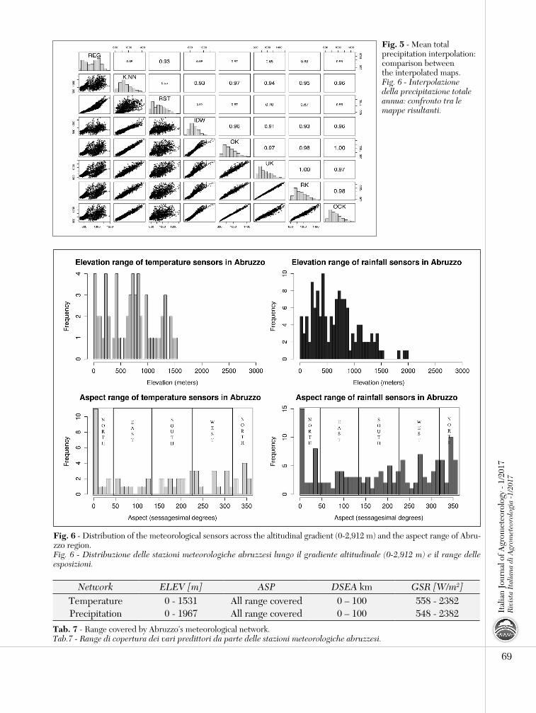
from central Europe and the Balkans (Di Lena and others 2013) enforce the complexity of interpolation. In addition, physiographic parameters are not the only driver. The circulation of air masses plays a fundamental role in climatological analysis (Bellucci et al., 2013) and, in this view, the spatial distribution of Abruzzo’s meteorological stations across the orographic range can be addressed as the main issue. Many studies demonstrated the importance of quantity of data for interpolation (Sluiter, 2009) but very few discussed about their distribution (Wong et al., 2004; Bhowmik and Costa, 2014). Abruzzo has a dense network (1 station every 100 km2 for precipitation and every 200 km2 for temperatures) but, nonetheless, the network is not well distributed (Tab. 7), following just a latitudinal-longitudinal gradient. In fact, even if all the aspects degrees are more or less covered, the higher elevations are not represented properly (Fig. 6). For this reason, more complex and time-consuming methods as OCK didn’t performed well and demonstrated that model’s complexity and prediction’s accuracy are not always correlated.In this study we also found that indices interpolation reduced both computational time and rRMSE. This happened because mathematical operation between climatic factors worked as data transformation which modified the relationships between dependent and independent variables. However, in such cases, a sensible loss of information is often necessary and must be considered and weighted.

concluSIonSWith the requirement of high spatial resolution maps, representativeness of climatic data is the main driving factor to obtain reliable prediction.

condition but on the opposite side of the Apennines chain (Latium region) lower RMSE were obtained (Attorre et al., 2007) with good correlation with the same physiographic parameters, ranking UK as the best interpolation method. Reasons rely on fact that Abruzzo, despite the relatively small extension, has a very particular orography, determining a high climatic variability without possibility to determine a specific connection among climatic data and physiographic parameters. The Abruzzo’s geographic position (Mediterranean area) and the elevation range (from sea level to 2912 m) nearby the coast which represent a barrier to continental winds and precipitations

Fig. 3 - Boxplots of rRMSE (rRMSE values are expressed in percentage/100). Circles represent the outliers.Fig. 3 - Boxplots dell’RMSE percentuale (valori espressi in percentuale/100). I cerchi rappresentano gli outliers.

Fig. 4 - Mean annual temperature interpolation: comparison between the interpolated maps.Fig. 5 - Interpolazione della temperatura media annua: confronto tra le mappe risultanti.

CIANO AGRO 1-17.indb 68 04/04/17 16.42

69

Ital

ian

Jour

nal o

f Agr

omet

eoro

logy

- 1/

2017

Riv

ista

Ita

liana

di A

grom

eteo

rolo

gia

-1/2

017

Fig. 6 - Distribution of the meteorological sensors across the altitudinal gradient (0-2,912 m) and the aspect range of Abru-zzo region.Fig. 6 - Distribuzione delle stazioni meteorologiche abruzzesi lungo il gradiente altitudinale (0-2,912 m) e il range delle esposizioni.

Fig. 5 - Mean total precipitation interpolation: comparison between the interpolated maps.Fig. 6 - Interpolazione della precipitazione totale annua: confronto tra le mappe risultanti.

Network ELEV [m] ASP DSEA km GSR [W/m2]Temperature 0 - 1531 All range covered 0 – 100 558 - 2382Precipitation 0 - 1967 All range covered 0 – 100 548 - 2382

tab. 7 - Range covered by Abruzzo’s meteorological network.Tab.7 - Range di copertura dei vari predittori da parte delle stazioni meteorologiche abruzzesi.

CIANO AGRO 1-17.indb 69 04/04/17 16.42

70

Ital

ian

Jour

nal o

f Agr

omet

eoro

logy

- 1/

2017

Riv

ista

Ita

liana

di A

grom

eteo

rolo

gia

-1/2

017

Bellucci A., Gualdi S., Masina S., Storto A., Scoccimarro E., Cagnazzo C., Fogli P., Manzini E., Navarra A., 2013. Decadal climate predictions with a coupled OAGCM initialized with oceanic reanalyses. Climate Dynamics, 40(5-6): 1483-1497. http://doi.org/10.1007/s00382-012-1468-z

Bhowmik A. K., Costa A. C., 2014. Represen-tativeness impacts on accuracy and precision of climate spatial interpolation in data-scarce regions. Meteorological Applications. http://doi.org/10.1002/met.1463

Bivand R., Keitt T., Rowlingson B., 2015. rgdal: Bindings for the Geospatial Data Abstraction Library. Retrieved from http://cran.r-project.org/package=rgdal

Blasi C., Chirici G., Corona P., Marchetti M., Maselli F., Puletti N., 2007. Spazializzazione di dati climatici a livello nazionale tramite modelli regressivi localizzati. Forest@, 4(2): 213-219. Retrieved from http://www.sisef.it/

Brunetti M., Maugeri M., Nanni T., Simolo C., Spinoni J., 2014. High-resolution temperature climatology for Italy: interpolation method intercomparison. International Journal of Climatology, 34(4): 1278-1296. http://doi.org/10.1002/joc.3764

Chai H., 2011. Analysis and comparison of spatial interpolation methods for temperature data in Xinjiang Uygur Autonomous Region, China. Natural Science, 03(12): 999-1010. http://doi.org/10.4236/ns.2011.312125

Cheaib A., BadeauV., Boe J., Chuine I., Delire C., Dufrêne E., François C., Gritti E.S., Legay M., Pagé C., Thuiller W., Viovy N., Leadley P., 2012. Climate change impacts on tree ranges: Model intercomparison facilitates understanding and quantification of uncertainty. Ecology Letters, 15(6): 533-544. http://doi.org/10.1111/j.1461-0248.2012.01764.x

Chiavetta U., Chirici G., 2008. Estimation of forest attributes by integration of inventory and remotely sensed data in Alto Molise. Italian Journal of Remote Sensing, 40(1): 89-106. Retrieved from http://server-geolab.agr.unifi.it/public/completed/2008_RIT_VOL40(1)_089_106_Chiavetta_et_al.pdf

Chirici G., Corona P., Marchetti M., Mastronardi A., Maselli F., Bottai L., Travaglini D., 2012. K-NN FOREST: A software for the non-parametric prediction and mapping of environmental variables by the k-Nearest Neighbors algorithm. European Journal of Remote Sensing, 45(1): 433-442. http://doi.org/10.5721/EuJRS20124536

Cover T., Hart P., 1967. Nearest Neighbor algorithm for learning with symbolic features. Machine Learning, 10: 57-78.

Consequently, when some parts of the study area are not covered by an adequate network (e.g. high elevations) results are not only inaccurate but also unknown.If statistical relationships between climatic factors and physiographic parameters is missing, also most complex and powerful algorithms fail. The interpolation of climatic and bioclimatic indices must be used very carefully. Even if time-consuming the reliability of maps must be considered, weighting also the nature of data. Temperature and precipitation data are often provided by different meteorological networks and can have different consistency. Anyway, in our opinion, interpolation of local data with geostatistic methods should be always preferred as well as the direct interpolation of the climatic indices because, in this case the interpolation errors (and uncertainties) could be reduced. Moreover among geostatistic family all methods estimates are highly correlated and the selection of the method do not constitute a critical issue. Differently among non-geostatistic method the selection can lead to a meaningful difference in the estimates.

AcKnowledgeMentSThis study has been carried out as part of the ABRFORGEN project (Implementation of forest nursery chain and organization of a modern management of forest genetic resources in Abruzzo), a partnership between the Forestry Research Centre of Consiglio per la ricerca in agricoltura e l’analisi dell’economia agraria and the Abruzzo Regional Government. Special thanks are due to Dr. Bruno Di Lena and Dr. Fabio Antenucci from Agricultural politics and rural development Management of Abruzzo Regional Government for climatic data and scientific support in the elaboration.

ReFeRenceSAkaike H., 1974. A new look at the statistical model

identification. IEEE Transactionson Automatic Control, 19(6): 716-723. http://doi.org/10.1109/TAC.1974.1100705.

Attorre F., Alfo M., De Sanctis M., Bruno F., 2007. Comparison of interpolation methods for mapping climatic and bioclimatic variables at regional scale. International Journal of Climatology, 1843(March): 1825-1843. http://doi.org/10.1002/joc

Attorre F., Francesconi F., Valenti R., Collalti A., Bruno F., 2008. Produzione di mappe climatiche e bioclimatiche mediante Universal Kriging con deriva esterna: teoria ed esempi per l’ Italia. Forest@, 5: 8-19.

CIANO AGRO 1-17.indb 70 04/04/17 16.42

71

Ital

ian

Jour

nal o

f Agr

omet

eoro

logy

- 1/

2017

Riv

ista

Ita

liana

di A

grom

eteo

rolo

gia

-1/2

017

C., 2008. Comparison of six methods for the interpolation of daily, European climate data. Journal of Geophysical Research: Atmospheres, 113(21). http://doi.org/10.1029/2008JD010100

Jones P. G., Thornton P. K., 2013. Generating downscaled weather data from a suite of climate models for agricultural modelling applications. Agricultural Systems, 114file://: 1-5. http://doi.org/10.1016/j.agsy.2012.08.002

Kao C. Y. S., Hung F. L. P., 2004. Twelve Dif-ferent Interpolation Methods: a Case Study. Proceedings of the XXth ISPRS Congress, 35: 778-785. Retrieved from http://www.isprs.org/proceedings/XXXV/congress/comm2/papers/231.pdf

Kottek M., Grieser J., Beck C., Rudolf B., Rubel F., 2006. World map of the Köppen-Geiger climate classification updated. Meteorologische Zeitschrift, 15(3): 259-263. http://doi.org/ 10.1127/0941-2948/2006/0130

Krige D., 1951. A statistical approach to some basic mine valuation problems on the Witwatersrand. Journal of Chemical, Metallurgical and Mining Society, 52(6): 119-139.

Kruskal W., Wallis W., 1952. Use of ranks in one-criterion variance analysis. Journal of the American Statistical Association, 47(260): 583-621.

Kurtzman D., Kadmon R., 1999. Mapping of temperature variables in Israel: A comparison of different interpolation methods. Climate Research, 13(1): 33-43. http://doi.org/10.3354/cr013033

Lasserre B., Chirici G., Chiavetta U., Garf?? V., Tognetti R., Drigo R., Di Martino P., Marchetti M., 2011. Assessment of potential bioenergy from coppice forests trough the integration of remote sensing and field surveys. Biomass and Bioenergy, 35(1): 716-724. http://doi.org/10.1016/j.biombioe.2010.10.013

Li J., Heap A. D., 2008. A Review of Spatial Interpolation Methods for Environmental Scientists. Australian Geological Survey Organisation, GeoCat# 68(2008/23): 154. http://doi.org/http://www.ga.gov.au/image_cache/GA12526.pdf

Mäkelä H., Pekkarinen A., 2004. Estimation of forest stand volumes by Landsat TM imagery and stand-level field-inventory data. Forest Ecology and Management, 196(2-3): 245-255. http://doi.org/10.1016/j.foreco.2004.02.049

Martinez-Meyer E., 2005. Climate change and biodiversity: some considerations in forecasting shifts in species’ potential distributions. Biodiversity Informatics, 2: 42-55.

Mátýas C., Vendramin G. G., Fady B., 2009. Forests at the limit: evolutionary - genetic consequences of environmental changes at the receding (xeric) edge of distribution. Report from a research workshop.

Dallal G. E., Wilkinson L., 1986. An analytic ap-proximation to the distribution of Lilliefors’ test for normality. The American Statistician, 40(4): 294-296.

Daly C., Halbleib M., Smith J. I., Gibson W. P., Doggett M. K., Taylor G. H., Curtis J., Pasteris P. P., 2008. Physiographically sensitive mapping of climatological temperature and precipitation across the conterminous United States. International Journal of Climatology, 28(15): 2031-2064. http://doi.org/10.1002/joc.1688

De Martonne E., 1927. Regions of interior basin drainage. Geographical Review, 17: 397-414.

Diodato N., Ceccarelli M., 2005. Interpolation processes using multivariate geostatistics for mapping of climatological precipitation mean in the Sannio Mountains (southern Italy). Earth Surface Processes and Landforms, 30(3): 259-268. http://doi.org/10.1002/esp.1126

Eischeid J. K., Pasteris P. a., Diaz H. F., Plantico M. S., Lott N. J., 2000. Creating a Serially Complete, National Daily Time Series of Temperature and Precipitation for the Western United States. Journal of Applied Meteorology, 39(9): 1580-1591. http://doi.org/10.1175/1520-0450(2000)039<1580:CASCND>2.0.CO;2

Emberger L., 1930. La vegetation de la region me-diterraneenne. Essai d’une classification des groupements vegetaux. Rev. Gen. Bot., 42(641-662): 705-721.

Franco-Lopez H., Ek A. R., Bauer M. E., 2001. Estimation and mapping of forest stand density, volume, and cover type using the k-nearest neighbors method. Remote Sensing of Environment, 77(3): 251-274. http://doi.org/10.1016/S0034-4257(01)00209-7

GRASS Development Team, 2015. Geographic Resources Analysis Support System (GRASS). Open Source Geospatial Foundation. Retrieved from http://grass.osgeo.org

Hijmans R. J., Cameron S. E., Parra J. L., Jones G., Jarvis A., 2005. Very high resolution interpolated climate surfaces for global land areas. International Journal of Climatology, 25(15): 1965-1978. http://doi.org/10.1002/joc.1276

Hijmans R. J., 2015. raster: Geographic Data Ana- lysis and Modeling. Retrieved from http : / /cran.r -project .org/package=raster Hofierka J., Parajka J., Mitasova H., Mitas L., 2002. Multivariate Interpolation of Precipitation Using Regularized Spline with Tension. Transactions in GIS, 6(2): 135-150. http://doi.org/10.1111/1467-9671.00101

Hofstra N., Haylock M., New M., Jones P., Frei

CIANO AGRO 1-17.indb 71 04/04/17 16.42

72

Ital

ian

Jour

nal o

f Agr

omet

eoro

logy

- 1/

2017

Riv

ista

Ita

liana

di A

grom

eteo

rolo

gia

-1/2

017

Schueler S., Falk W., Koskela J., Lefèvre F., Bozzano M., Hubert J., Kraigher H., Longauer R., Olrik D. C., 2014. Vulnerability of dynamic genetic conservation units of forest trees in Europe to climate change. Global Change Biology, 20(5): 1498-1511. http://doi.org/10.1111/gcb.12476

Schuurmans J. M., Bierkens M. F. P., Pebesma E. J., Uijlenhoet R., 2007. Automatic Prediction of High-Resolution Daily Rainfall Fields for Multiple Extents: The Potential of Operational Radar. Journal of Hydrometeorology, 8(6): 1204-1224. http://doi.org/10.1175/ 2007JHM792.1

Sharif M., Burn D. H., Wey K. M., 2007. Daily and Hourly Weather Data Generation using a K-Nearest Neighbour Approach. 18th Canadian Hydrotechnical Conference, 1-10.

Sluiter R., 2009. Interpolation methods for climate data: literature review. KNMI, R&D Information and Observation Technology, 1-28.

Vacchiano G., Motta R., 2014. An improved species distribution model for Scots pine and downy oak under future climate change in the NW Italian Alps. Annals of Forest Science. http://doi.org/10.1007/s13595-014-0439-4

Van Houwelingen J., Le Cressie S., 1990. Predictive value of statistical models. Statistics in Medicine, 9: 1303-1325.

Wang T., Hamann A., Spittlehouse D. L., Murdock T. Q., 2012. ClimateWNA-high-resolution spatial climate data for western North America. Journal of Applied Meteorology and Climatology, 51(1): 16-29. http://doi.org/10.1175/JAMC-D-11-043.1

Wilks D. S., 2011. Statistical Methods in the Atmospheric Sciences International Geophysics (Vol. 100). http://doi.org/10.1016/B978-0-12-385022-5.00015-4

Wong D. W., Yuan L., Perlin S. a, 2004. Comparison of spatial interpolation methods for the estimation of air quality data. Journal of Exposure Analysis and Environmental Epidemiology, 14(5): 404-415. http://doi.org/10.1038/sj.jea.7500338

Xia Y., Fabian P., Stohl A., Winterhalter M., 1999. Forest climatology: Estimation of missing values for Bavaria, Germany. Agricultural and Forest Meteorology, 96(1-3): 131-144. http://doi.org/10.1016/S0168-1923(99)00056-8

Yates D., 2003. A technique for generating regional climate scenarios using a nearest-neighbor algorithm. Water Resources Research, 39(7): 1-15. http://doi.org/10.1029/2002WR001769

Yilmaz O. Y., Tolunay D., 2012. Distribution of the major forest tree species in Turkey within spatially interpolated plant heat and hardiness zone maps. IForest, 5(APRIL): 83-92. http://doi.org/10.3832/ifor0611-005

Annals of Forest Science, 66(8): 800-800. http://doi.org/10.1051/forest/2009081

Mitas L., Mitasova H., 1999. Spatial Interpolation. Geographical, 36(3): 481-492. http://doi.org/10. 2307/2533421

Odeh I. O. A., McBratney A. B., Chittleborough D. J., 1995. Further results on prediction of soil properties from terrain attributes: heterotopic cokriging and regression-kriging. Geoderma, 67(3-4): 215-226. http://doi.org/10.1016/0016-7061(95)00007-B

Parmesan C., 1996. Climate and species’ range. Nature. http://doi.org/10.1038/382765a0

Paulhus J. L. H., Kohler M. A., 1952. Interpolation of missing precipitation records. Monthly Weather Review, 80(8): 129-133. http://doi.org/10.1175/1520-0493(1952)080<0129:IOMPR>2.0.CO;2

Pearson R. G., Dawson T. P., 2003. Predicting the impacts of climate change on the distribution of speces: are bioclimate envelope models useful? Global Ecology and Biogeography, 12: 361-371. Retrieved from <Go to ISI>://000185105800001

Pebesma E. J., 2004. Multivariable geostatistics in S: The gstat package. Computers and Geosciences, 30(7): 683-691. http://doi.org/ 10.1016/j.cageo.2004.03.012

Pellatt M. G., Goring S. J., Bodtker K. M., Cannon A. J., 2012. Using a down-scaled bioclimate envelope model to determine long-term temporal connectivity of Garry oak (Quercus garryana) habitat in western North America: implications for protected area planning. Environmental Management, 49(4): 802-815. http://doi.org/10.1007/s00267-012-9815-8

Provan J., Maggs C. A., 2012. Unique genetic variation at a species’ rear edge is under threat from global climate change. Proceedings. Biological Sciences / The Royal Society, 279(1726): 39-47. http://doi.org/10.1098/rspb.2011.0536

R CoreTeam, 2015. R: A language and environment for statistical computing. R Foundation for Statistical Computing, Vienna, Austria: https://www.R-project.org/. Retrieved from https://www.r-project.org

Ramos Calzado P., Gómez Camacho J., Pérez Bernal F., Pita López M. F., 2008. A novel approach to precipitation series completion in climatological datasets: application to Andalusia. International Journal of Climatology, 28(11): 1525-1534. http://doi.org/10.1002/joc

Rivas-Martinez S., 1996. Clasificacıon Bioclimatica de la tierra. Folia Botanica Matritensis, 16: 1-32. Schneider T., 2001. Analysis of incomplete climate data: Estimation of Mean Values and covariance matrices and imputation of Missing values. Journal of Climate, 14(5): 853-871. http://doi.org/10.1175/1520-0442(2001)014<0853:AOICDE>2.0.CO;2

CIANO AGRO 1-17.indb 72 04/04/17 16.42