does central bank communication really lead to better ... central bank communication really lead to...

ORI GIN AL PA PER

Does central bank communication really lead to betterforecasts of policy decisions? New evidence basedon a Taylor rule model for the ECB

Jan-Egbert Sturm • Jakob De Haan

Published online: 6 November 2010

� The Author(s) 2010. This article is published with open access at Springerlink.com

Abstract Nowadays, it is widely believed that greater disclosure and clarity over

policy may lead to greater predictability of central bank actions. We examine whether

communication by the European Central Bank (ECB) adds information compared to

the information provided by a Taylor rule model in which real-time expected inflation

and output growth are used. We use five indicators of ECB communication that are all

based on the ECB President’s introductory statement at the press conference following

an ECB policy meeting. Our results suggest that even though the indicators are

sometimes quite different from one another, they add information that helps predict the

next policy decision of the ECB. Furthermore, also when the interbank rate is included

in our Taylor rule model, the ECB communication indicators remain significant.

Keywords ECB � Central bank � Communication � Taylor rule

JEL classification E52 � E53 � E3

J.-E. Sturm � J. De Haan

KOF Swiss Economic Institute, ETH Zurich, Zurich, Switzerland

J. De Haan

De Nederlandsche Bank (DNB), Amsterdam, The Netherlands

J.-E. Sturm � J. De Haan

CESifo Munich, Munich, Germany

J. De Haan (&)

Faculty of Economics and Business, University of Groningen,

PO Box 800, 9700 AV Groningen, The Netherlands

e-mail: [email protected]

123

Rev World Econ (2011) 147:41–58

DOI 10.1007/s10290-010-0076-4

1 Introduction

Since monetary policy is increasingly becoming the art of managing expectations,

communication has developed into a key instrument in the central bankers’ toolbox.

Greater disclosure and clarity over policy may lead to greater predictability of

central bank actions, which, in turn, reduces uncertainty in financial markets.

Nowadays, there is a strongly held belief among central bankers that a high degree

of predictability is important. According to Poole (2001, p. 9), ‘‘The presumption

must be that market participants make more efficient decisions … when markets can

correctly predict central bank actions.’’ Communication may also enhance the

effectiveness of monetary policy.

The extent to which central bank communication has been successful is very

much an empirical issue. Therefore, it is no surprise that the empirical literature on

central bank communication has seen major developments in recent years.1 Many of

these studies refer to the communication policy of the European Central Bank

(ECB). There is substantive evidence that ECB communication moves financial

markets in the intended direction (see, for instance, Ehrmann and Fratzscher 2007;

Musard-Gies 2006; Brand et al. 2006). There is also a consensus that ECB

communication increases the predictability of interest decisions by the ECB (De

Haan 2008). The ECB tries to prepare markets for upcoming interest rate decisions

using its communication policy. So, ECB communication contains some forward

guidance and may have predictive power. Even in the absence of forward guidance,

central bank communication variables can meaningfully enter a Taylor (1993) rule

model: with only inflation and output included, a Taylor rule model is very likely to

be mis-specified, since central banks typically base their interest rate decisions on

many more economic variables. If the ECB President gives the overall assessment

of the economic situation based on all the variables that the ECB looks at, central

bank communication might be a very useful way to summarise this information

content in a very parsimonious fashion.

However, there is disagreement in the literature about the extent to which ECB

communication adds information compared to the information contained by macro-

economic variables that are typically included in a Taylor rule model. For instance,

whereas Heinemann and Ullrich (2007) and Rosa and Verga (2007) conclude that

communication adds information not provided by these macroeconomic variables,

Jansen and De Haan (2009) find that straightforward Taylor rule models outperform

models using only communication indicators.

The purpose of this paper is to re-examine to what extent ECB communication adds

information compared to the information provided by a Taylor rule model in which

expected inflation and output growth are used when forecasting upcoming interest rate

decisions. There are some important differences between our study and previous

research. First, Heinemann and Ullrich (2007) and Rosa and Verga (2007) estimated

backward-looking Taylor rule specifications. However, as Svensson (2003) has

shown, even if the ultimate objective of monetary policy is to stabilize inflation and

output, a simple Taylor rule will not be optimal in a reasonable macroeconomic model.

1 See Blinder et al. (2008) for an extensive survey. See also Ehrmann and Fratzscher (2009).

42 J.-E. Sturm, J. De Haan

123

Interest rate changes affect inflation and output with a sizable lag. Therefore, monetary

policy has to be forward-looking. Some recent studies suggest that the use of expected

inflation and output growth lead to very different results than backward-looking

Taylor rule models for the ECB (Sauer and Sturm 2007; Gorter et al. 2008).2 For

instance, Gorter et al. (2008) report that in their backward-looking Taylor model the

Taylor principle does not hold, in contrast to the Taylor model with expected inflation

and output growth. So the findings of Heinemann and Ullrich (2007) and Rosa and

Verga (2007) may just reflect their use of a potentially mis-specified Taylor rule

model. Jansen and De Haan (2009) employed a similar forward-looking Taylor rule

model as used in the present paper and conclude that their communication indicator

does not increase the fit of the model.3

Second, all previous papers use just one indicator of ECB communication.

Whereas Heinemann and Ullrich (2007) and Rosa and Verga (2007) use

communication indicators that are based on the introductory statement of the

ECB’s President at the press conference following the ECB policy meeting, Jansen

and De Haan (2009) employ an indicator based on Bloomberg news reports. We will

show that even if various communication indicators are based on the same

information, i.e. the speech of the ECB’s President after the policy meeting, they

give very different signals about the direction of the ECB monetary policy. In order

to test to what extent results are sensitive to the choice of a particular indicator, we

employ five different indicators of ECB communication that are all based on the

ECB President’s introductory statement at the press conference following an ECB

policy meeting. Apart from the indicators of Heinemann and Ullrich (2007) and an

updated version of the index of Rosa and Verga (2007), we employ the aggregate

index of Berger et al. (2010), the KOF Monetary Policy Communicator (MPC) as

published by the KOF Swiss Economic Institute, and the indicator of Ullrich (2008).

Our main finding is that ECB communication turns out to be significant in our

Taylor rule model. In other words, it is worthwhile for financial market participants

to read the ECB President’s lips, as this adds information about upcoming interest

rate decisions that is not provided by expected inflation and expected output growth.

This conclusion holds for most communication indicators. We include the interbank

rate to control for financial markets forecast of future ECB monetary policy moves

(e.g. Bernoth and von Hagen 2004). Even in this specification, the ECB

communication indicators remain significant. Using Brier scores and the ranked

probability scores, we conclude that Taylor rule models that include ECB

communication indicators outperform models without those indicators in terms of

their out-of-sample forecasting abilities.

The paper is organised as follows. Section 2 outlines the model, while Sect. 3

describes the data. Section 4 presents the results and Sect. 5 offers the conclusions.

2 In some specifications of his policy reaction function for the ECB, also Gerlach (2007) uses expected

inflation and expected output growth. His estimates differ substantially from those of Sauer and Sturm

(2007) and Gorter et al. (2008). Gerlach concludes, for instance, that inflation is not significant in his

Taylor rule model for the ECB.3 Another possible reason why Jansen and De Haan (2009) come to different conclusions than

Heinemann and Ullrich (2007) and Rosa and Verga (2007) is that their sample period refers to 1999–2002

only. They also use a different communication variable.

New evidence based on a Taylor rule model for the ECB 43

123

2 The model

According to the Taylor rule, in setting its policy instrument (it) the central bank

should react to deviations of inflation (pt) from its target (p*) and to deviations of

output (yt) from potential (y*):

it ¼ ðr � þp�Þ þ bðpt � p�Þ þ c yt � y�ð Þ; ð1Þ

where r* is the neutral real interest rate, and c[ 0, b[ 1.4 As the ECB is known

not to focus on the output gap (Gerlach 2007), probably in view of the difficulty to

measure it in a real time situation, we estimate a Taylor rule using output growth.

Walsh (2004) and Gerberding et al. (2005) argue that such a rule performs well in

the presence of imperfect information. We assume a constant potential growth rate

and include D(yt - y*) instead of (yt - y*):

it ¼ ðr � þp�Þ þ bðpt � p�Þ þ c Dyt � Dy�ð Þ: ð2ÞMost previous studies that estimated a Taylor rule for the ECB used data for the

actual (ex-post) inflation rate and the output gap. Svensson (2003) has shown that

even if the ultimate objective of monetary policy is to stabilize inflation and output,

a simple Taylor rule will not be optimal in a reasonable macroeconomic model.

Because interest rate changes affect inflation and output with a sizable lag, monetary

policy has to be forward-looking. Sauer and Sturm (2007) and Gorter et al. (2008)

therefore estimate Taylor rules using forward-looking (and real-time) data.

Similarly, our model is defined as:

it ¼ ðr � þp�Þ þ bðEtptþ12 � p�Þ þ cðEtDytþ12 � Dy�Þ; ð3Þ

where Et is the expectations operator and the time index now refers to months.5

Generally, central banks adjust interest rates in small steps to the target rate itT

(often referred to as interest rate smoothing), so that we can write:

iTt ¼ ðr � þp�Þ þ bðEtptþ12 � p�Þ þ cðEtDytþ12 � Dy�Þ: ð4Þ

The actual interest rate, it, adjusts only slowly to this target, i.e.:

it ¼ qit�1 þ ð1� qÞiTt þ vt ð5Þ

or

Dit ¼ ð1� qÞ iTt � it�1

� �þ vt; ð6Þ

where q denotes the smoothing parameter and vt = dvt-1 ? et. The observed inertia

may also be explained by serially correlated error terms in the policy rule (omitted

shocks like financial crises) (see Rudebusch 2002).

4 According to the ‘‘Taylor principle’’, b[ 1, i.e. if inflation increases the nominal interest rate must

increase more (Di [Dp) in order to raise the real rate.5 Data restrictions force us to use a lead of 12 months.


123

3 Data

Our data refer to the euro area over the period 1999–2007, although some ECB

communication indicators are only available for a shorter period. Our dependent

variable is the Main Refinancing Rate (MRR) as determined by the ECB Governing

Council (source: ECB). Real-time expected inflation and output growth time series

have been constructed from Consensus Economics forecasts. These forecasts are used

as a proxy for the ECB’s expectations of inflation and output growth. The Consensus

data are unique, not revised and, consequently, not subject to the real-time critique of

Orphanides (2001).6 Every month, major banks and forecast institutes in the EMU-

countries give their forecasts for the near future, i.e. the current and the next year. Euro

area expected inflation and gross domestic product (GDP) growth series are

constructed from these forecasts for all euro area countries except Luxembourg.7 As

Consensus Economics did not collect euro area forecasts before December 2002, we

use country-specific forecasts, which are weighted by their share of GDP in the euro

area GDP.

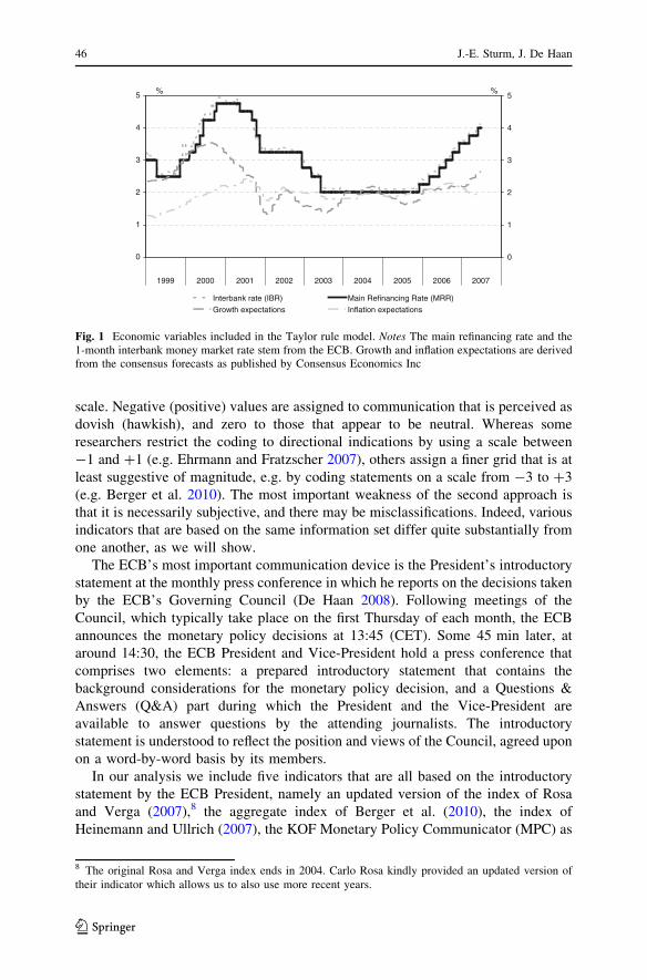
Figure 1 shows the MRR and expected inflation and expected output growth. In

addition, the one-month Interbank Rate (IBR) is shown (source: ECB). As part of

our robustness analysis, the difference between the MRR and the IBR is included as

an additional control variable. Not surprisingly, both interest rates move closely

together. Expected output growth and the MRR also move together to some extent,

while the co-movement of expected inflation and the MRR seems to be limited since

expected inflation hovers around the ECB’s medium term objective of an inflation

rate below, but close to 2%.

Various approaches have been developed in the literature to measure (the effects

of) central bank communication (see Blinder et al. 2008 for more details). Starting

with Kohn and Sack (2004), various studies have examined the effects of central

bank communication events on the volatility of financial variables. The basic idea is

that, if communication affects the returns on financial assets, the volatility of these

returns should be higher on days of central bank communication, ceteris paribus,

because the signals contain ‘‘news.’’ Focusing on volatility makes it unnecessary to

assign a direction to each statement. The most important weakness of this approach

is that it cannot assess whether markets moved in the ‘‘right’’ direction. In other

words, the Kohn and Sack approach may establish that central bank communication

creates news, but it is unable to determine whether it reduces noise.

In another approach, communication is quantified in order to assess both the

direction and magnitude of its effects on asset prices—and thus to determine to what

extent communication has its intended effects. Communication must be classified

according to their content and/or likely intention, and then coded on a numerical

6 Orphanides (2001) has shown that the use of real-time instead of ex post data leads to very different

estimated coefficients in Taylor rule models for the Federal Reserve.7 To convert the reported growth rates into monthly moving figures, we take as the 12-month forecast the

weighted average of the forecast for the current and the following year, where the weights are x/12 for the

x remaining months in the current year and (12 - x)/12 for the following year’s forecast. As the survey is

conducted at the beginning of each month, we consider the current month to belong to the remaining

months in the current year.


123

scale. Negative (positive) values are assigned to communication that is perceived as

dovish (hawkish), and zero to those that appear to be neutral. Whereas some

researchers restrict the coding to directional indications by using a scale between

-1 and ?1 (e.g. Ehrmann and Fratzscher 2007), others assign a finer grid that is at

least suggestive of magnitude, e.g. by coding statements on a scale from -3 to ?3

(e.g. Berger et al. 2010). The most important weakness of the second approach is

that it is necessarily subjective, and there may be misclassifications. Indeed, various

indicators that are based on the same information set differ quite substantially from

one another, as we will show.

The ECB’s most important communication device is the President’s introductory

statement at the monthly press conference in which he reports on the decisions taken

by the ECB’s Governing Council (De Haan 2008). Following meetings of the

Council, which typically take place on the first Thursday of each month, the ECB

announces the monetary policy decisions at 13:45 (CET). Some 45 min later, at

around 14:30, the ECB President and Vice-President hold a press conference that

comprises two elements: a prepared introductory statement that contains the

background considerations for the monetary policy decision, and a Questions &

Answers (Q&A) part during which the President and the Vice-President are

available to answer questions by the attending journalists. The introductory

statement is understood to reflect the position and views of the Council, agreed upon

on a word-by-word basis by its members.

In our analysis we include five indicators that are all based on the introductory

statement by the ECB President, namely an updated version of the index of Rosa

and Verga (2007),8 the aggregate index of Berger et al. (2010), the index of

Heinemann and Ullrich (2007), the KOF Monetary Policy Communicator (MPC) as

0

1

2

3

4

5

0

1

2

3

4

5

1999 2000 2001 2002 2003 2004 2005 2006 2007

Interbank rate (IBR) Main Refinancing Rate (MRR)

Growth expectations Inflation expectations

% %

Fig. 1 Economic variables included in the Taylor rule model. Notes The main refinancing rate and the1-month interbank money market rate stem from the ECB. Growth and inflation expectations are derivedfrom the consensus forecasts as published by Consensus Economics Inc

8 The original Rosa and Verga index ends in 2004. Carlo Rosa kindly provided an updated version of

their indicator which allows us to also use more recent years.


123

published by the KOF Swiss Economic Institute and used by Conrad and Lamla

(2007),9 and the indicator of Ullrich (2008).10 All data used in the present paper are

available.11

Different from the other indicators, the KOF MPC is based on the

interpretation of the introductory statements by the ECB President by Media

Tenor, a media research institute. Media analysts read the text of the introductory

statement of the monthly press conference sentence by sentence and code them.

The coding is aggregated by the KOF Swiss Economic Institute into an index by

taking balances of the statements that reveal that the ECB sees upside risks to

future price stability and statements that reveal that the ECB sees downside risks

to future price stability, relative to all statements about future price stability

(including neutral ones). Hence, in contrast to the other communication

indicators we consider, it only takes forward-looking statements into account.

By construction, the values of the KOF MPC are restricted to be in the range of

minus one to plus one. The larger a positive (negative) value of the KOF MPC,

the stronger the ECB communicated that there are upside (downside) risks for

future price stability.

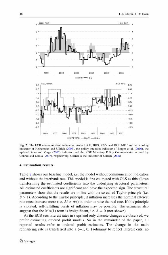
Figure 2 shows the various ECB communication indicators that we use, while

Table 1 shows the correlation of the various indicators. It becomes clear that the

indicators are sometimes quite different from one another. Whereas the correlation

coefficients amongst the first three indicators compiled by economists are around

0.8, their correlation with the KOF MPC is more modest.12

The next step in our analysis is to estimate a forward-looking Taylor rule model

for the ECB and to augment this model with the ECB communication indicators

outlined above.13 As we start with daily information, we need to decide at which

moment in time to forecast the next interest rate decision. Two moments in time

appear natural: (i) at the day of and directly after the previous policy decision, and

(ii) the day the new Consensus forecasts are released (see Fig. 3). At that day, there

is new information on expected inflation and expected growth. We have decided to

focus on the second option as it will be the hardest test for the ECB communication

indicators to have any affect at all. After all, in this set-up information provided by

the ECB communication is already captured in the Consensus forecasts and the

interbank rate.

9 Available at: http://www.kof.ethz.ch/communicator.10 Katrin Ullrich kindly provided her indicator. Other ECB communication indicators (like that of Jansen

and De Haan 2009) are based on other communication devices and are therefore not included. The index

of Musard-Gies (2006) is only available for a short period and is therefore not included.11 See www.kof.ethz.ch/wp236.12 We have also applied a principal components analysis on the various indicators. The first principal

component explains almost 68% of the variance of the individual indicators. In line with Table 1, the

correlation of the KOF MPC with the principal component is only 0.50.13 Using a different methodology that we cannot employ due to lack of sufficient variability of our

interest rate data, Kim et al. (2008) also estimate various Taylor rule models in their analysis of the

predictability of interest rate decisions by the Bank of England. These authors do not include central bank

communication in their model.


123

http://www.kof.ethz.ch/communicator

http://www.kof.ethz.ch/wp236

4 Estimation results

Table 2 shows our baseline model, i.e. the model without communication indicators

and without the interbank rate. This model is first estimated with OLS as this allows

transforming the estimated coefficients into the underlying structural parameters.

All estimated coefficients are significant and have the expected sign. The structural

parameters show that the results are in line with the so-called Taylor principle (i.e.

b[ 1). According to the Taylor principle, if inflation increases the nominal interest

rate must increase more (i.e. Di [ Dp) in order to raise the real rate. If this principle

is violated, self-fulfilling bursts of inflation may be possible. The estimates also

suggest that the MA(1) term is insignificant, i.e. d = 0 (not shown).

As the ECB sets interest rates in steps and only discrete changes are observed, we

prefer estimating ordered probit models. So in the remainder of the paper, all

reported results refer to ordered probit estimates. The change in the main

refinancing rate is transferred into a (-1, 0, 1)-dummy to reflect interest cuts, no

-2

-1

0

1

2

3

4

1999 2000 2001 2002 2003 2004

-2

-1

0

1

2

3

4

BHS H & U

H&U, BHS H&U, BHS

-2.5

-2.0

-1.5

-1.0

-0.5

0.0

0.5

1.0

1.5

2.0

2.5

1999 2000 2001 2002 2003 2004 2005 2006 2007

-1.25

-1.00

-0.75

-0.50

-0.25

0.00

0.25

0.50

0.75

1.00

1.25

KOF MPC R & V Ullrich

R&V, Ullrich KOF MPC

Fig. 2 The ECB communication indicators. Notes H&U, BHS, R&V and KOF MPC are the wordingindicator of Heinemann and Ullrich (2007), the policy intention indicator of Berger et al. (2010), theupdated Rosa and Verga (2007) indicator, and the KOF Monetary Policy Communicator as used byConrad and Lamla (2007), respectively. Ullrich is the indicator of Ullrich (2008)


123

changes, and interest rate increases.14 The final column of Table 2 shows the

ordered probit results for the baseline model. They are similar to the OLS estimates.

Tables 3 and 4 show the estimation results if we add the various ECB

communication indicators. In each regression we use the maximum number of

observations possible. However, the conclusions are the same if we restrict the

sample to those 64 observations (basically the 1999–2004 period) for which all

indicators are available (results are available on request). The difference between

both tables is that in Table 4 also the one-month interbank rate is included as

explanatory variable to control for financial markets forecast of future ECB

monetary policy moves. If markets were efficient, all available information,

Table 1 Correlation matrix

(1) (2) (3) (4) (5) (6) (7) (8) (9)

(1) MRR -0.08 0.41 0.62 0.16 – -0.15 – -0.05

(2) IBRt=CF - MRR -0.08 – -0.21 0.32 0.32 – 0.26 – 0.06

(3) Inflation exp. 0.56 -0.25 – 0.02 0.28 – 0.18 – 0.18

(4) Growth exp. 0.59 0.34 0.07 – 0.55 – 0.21 – 0.16

(5) R&V 0.30 0.36 0.12 0.76 – – 0.68 – 0.48

(6) H&U 0.26 0.29 0.16 0.70 0.75 – – – –

(7) Ullrich -0.06 0.31 0.07 0.42 0.62 0.70 – – 0.39

(8) BHS 0.32 0.40 0.17 0.78 0.88 0.79 0.61 – –

(9) KOF MPC -0.04 0.05 0.08 0.21 0.41 0.33 0.33 0.28 –

The correlation coefficients reported in italics (lower-left triangle) use a fixed sample of 68 observations

during the period 1999–2004. Each of the correlation coefficients reported in the upper-right part use the

96 observations, which cover the period from January 1999 until June 2007

Council meeting

interest rate decision

press communiqué

Next Councilmeeting

Release consensus

inflation expectations

growth expectations

New interest rate decision

time

Approximately one month

Release consensus

inflation expectations

growth expectations

Fig. 3 The timing in our model

14 This choice is motivated by the fact that only in a few cases the interest rate was moved by 50 basis

points (in either direction). Hence, it is statistically difficult to distinguish between the case of a 25 and a

50 basis point move. The results do not change in any meaningful way in case we distinguish between 50

and 25 basis point changes.


123

including the ECB communication, should be reflected in asset prices. In that case,

the ECB communication indicators should become insignificant.

Two conclusions can be drawn from our estimations. First, in line with the results

of Heinemann and Ullrich (2007) and Rosa and Verga (2007), the coefficients of the

ECB communication indicators are significantly different from zero, although in

some cases only at the 10% level, except for the KOF MPC. However, according to

the KOF MPC, the ECB already starts preparing the general public for interest rate

changes more than 1 meeting in advance. Once it is lagged by one period, the KOF

MPC turns significant, while the lag of the other indicators is not significant.

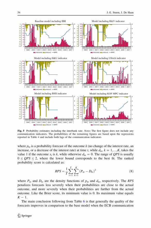
Second, also if the interbank rate is included, the ECB communication indicators

remain significant. The latter result implies that the interbank interest rate, although

it is always significant, does not contain all the information provided by the

communication indicators. Figures 4 and 5 show the implied probabilities of the

estimates reported in Tables 3 and 4, respectively.

As both figures show, the estimated probabilities quite heavily depend upon these

indicators. Estimates of the marginal effects confirm this. For instance, a one

standard deviation increase in the value of the Rosa and Verga indicator (while

keeping the other explanatory variables equal to their means) increases the

probability of an interest rate hike by close to 13.5 percentage points.

As suggested by one of the referees, we have also estimated a slightly different

model using different forecasting horizons.

iTtþj ¼ ðr � þp�Þ þ bðEtptþ12 � p�Þ þ cðEtDytþ12 � Dy�Þ: ð40Þ

Ditþj ¼ ð1� qÞ iTtþj � it�1

� �þ vt; j ¼ 0; 1; 2; 3 ð60Þ

j ¼ 0; 1; 2; 3

Table 2 Baseline model: OLS and ordered probit models

OLS

(1)

Implied structural

parameters

(2)

Ordered

Probit

(3)

MRRt-1 -0.109***

(-3.53)

q 0.891***

(28.96)

-1.048***

(-4.06)

Inflation exp.t=CF 0.154*

(1.74)

b 1.414**

(2.12)

1.700**

(2.50)

Growth exp.t=CF 0.187***

(4.18)

c 1.725***

(6.35)

1.756***

(4.93)

Constant -0.381**

(-2.31)

r* 0.766***

(5.25)

Observations 96 96

R-squared 0.225

Log likelihood 47.97 -54.20

The sample uses all observations available during the period 1999–2007 (June). In columns (1) and (2)

t-statistics are in parentheses. In column (3) robust z-statistics are in parentheses

***, ** and * indicate significance at the level of 1, 5 and 10%, respectively


123

Tab

le3

Ord

ered

pro

bit

resu

lts

wit

hE

CB

com

munic

atio

nin

dic

ators

added

R&

V

(1)

H&

U

(2)

Ull

rich

(3)

BH

S

(4)

MP

C

(5)

R&

V

(6)

H&

U

(7)

Ull

rich

(8)

BH

S

(9)

MP

C

(10

)

MR

Rt-

1-

0.7

40

**

(-2

.261

)

-0

.995

**

*

(-2

.73

6)

-0

.61

6*

*

(-2

.208

)

-1

.009

**

(-2

.478

)

-0

.993

**

*

(-3

.63

9)

-0

.74

8*

*

(-2

.24

5)

-0

.979

**

(-2

.516

)

-0

.776

**

*

(-2

.694

)

-0

.965

**

(-2

.42

4)

-0

.86

4*

**

(-2

.999

)

Infl

atio

nex

p. t=

CF

-0

.153

(-0

.190

)

0.1

21

(0.1

06)

0.6

11

(0.7

75)

-0

.554

(-0

.561

)

1.4

86

**

(2.2

40)

-0

.15

3

(-0

.18

4)

-0

.285

(-0

.212

)

1.0

89

(1.2

82)

-0

.502

(-0

.49

7)

1.0

43

(1.3

57

)

Gro

wth

exp

. t=C

F0

.66

9

(1.3

72

)

1.5

85

**

*

(2.6

23)

1.3

16

**

*

(3.2

01)

0.5

74

(1.0

33

)

1.6

93

**

*

(4.3

57)

0.6

65

(1.3

47)

1.2

85

**

(2.0

11

)

1.5

47

**

*

(3.5

09)

0.6

17

(1.1

09)

1.4

94

**

*

(3.7

41

)

Co

mm

.in

d. t-

11

.13

1*

**

(3.8

91

)

0.4

51

*

(1.8

12)

1.1

89

**

*

(3.9

09)

1.6

13

(3.1

88

)

0.7

64

(0.9

72)

1.0

99

**

*

(3.1

70)

0.4

59

*

(1.8

46

)

1.3

79

**

*

(3.6

73)

1.7

17

**

*

(2.8

57)

0.7

61

(0.9

86

)

Co

mm

.in

d. t-

20

.047

(0.1

63)

0.3

11

(1.2

33

)

-0

.519

*

(-1

.687

)

-0

.210

(-0

.48

1)

1.9

28

**

*

(2.6

23

)

Obse

rvat

ions

96

68

96

68

96

95

67

95

67

95

Lo

gli

kel

iho

od

-4

1.9

1-

30

.81

-4

5.4

5-

23

.64

-5

3.6

8-

41

.87

-3

0.0

5-

44

.16

-2

3.5

4-

50

.62

Rob

ust

z-st

atis

tics

inp

aren

thes

es

***,

**

and

*in

dic

ate

signifi

cance

atth

ele

vel

of

1,

5an

d10%

,re

spec

tivel

y


123

Tab

le4

Ord

ered

pro

bit

resu

lts

incl

udin

gco

mm

unic

atio

nin

dic

ators

and

the

inte

rban

kra

te

R&

V

(1)

H&

U

(2)

Ull

rich

(3)

BH

S

(4)

MP

C

(5)

R&

V

(6)

H&

U

(7)

Ull

rich

(8)

BH

S

(9)

MP

C

(10

)

MR

Rt-

1-

0.4

06

(-1

.157

)

-0

.850

**

(-2

.34

1)

-0

.44

1

(-1

.566

)

-1

.142

**

(-2

.22

0)

-0

.74

7*

**

(-2

.676

)

-0

.407

(-1

.147

)

-0

.85

3*

*

(-2

.23

4)

-0

.62

8*

*

(-2

.031

)

-1

.120

**

(-2

.362

)

-0

.610

**

(-2

.100

)

IBR

t=C

F-

MR

Rt-

16

.278

**

(2.0

20

)

7.2

84

**

*

(2.5

86)

6.9

90

**

*

(2.5

84)

7.4

52

**

*

(2.7

74)

6.9

51

**

(2.3

42)

6.2

66

**

(2.0

14

)

7.4

00

**

*

(2.6

59)

7.5

33

**

*

(2.8

87)

7.4

14

**

*

(2.7

52

)

6.8

58

**

(2.1

36

)

Infl

atio

nex

p. t=

CF

0.1

07

(0.1

23

)

0.6

21

(0.5

23)

1.1

79

(1.4

55)

0.4

77

(0.4

66)

1.8

71

**

*

(2.8

17)

0.0

83

(0.0

90

5)

0.7

04

(0.5

30)

1.8

06

**

(2.0

83)

0.4

92

(0.4

75

)

1.3

80

*

(1.8

94

)

Gro

wth

exp

. t=C

F-

0.0

46

(-0

.084

)

1.0

31

*

(1.6

86)

0.8

12

*

(1.9

49)

0.3

69

(0.6

38)

1.1

36

**

*

(2.7

78)

-0

.058

(-0

.103

)

1.0

71

(1.5

02)

1.0

68

**

(2.2

76)

0.3

76

(0.6

40

)

0.9

34

**

(2.2

84

)

Co

mm

.in

d. t-

11

.125

**

*

(3.9

93

)

0.6

18

*

(1.6

86)

1.2

53

**

*

(3.8

16)

1.7

77

**

*

(3.3

75)

0.9

64

(1.0

68)

1.0

97

**

*

(3.1

89

)

0.6

12

*

(1.6

89)

1.5

18

**

*

(3.3

78)

1.8

06

**

*

(2.8

91

)

0.9

48

(1.0

74

)

Co

mm

.in

d. t-

20

.044

(0.1

53

)

-0

.04

8

(-0

.18

2)

-0

.74

1*

*

(-2

.186

)

-0

.068

(-0

.130

)

1.8

80

**

*

(2.6

71

)

Obse

rvat

ions

96

68

96

68

96

95

67

95

67

95

Lo

gli

kel

ihoo

d-

35

.53

-2

3.4

7-

37

.73

-1

8.1

0-

45

.00

-3

5.5

0-

23

.44

-3

5.7

1-

18

.09

-4

2.7

5

Rob

ust

z-st

atis

tics

inp

aren

thes

es

***,

**

and

*in

dic

ate

signifi

cance

atth

ele

vel

of

1,

5an

d10%

,re

spec

tivel

y


123

The results, shown in Table 5, suggest that the communication variables remain

significant. In line with our previous findings, the KOF indicator only becomes

significant if j [ 0.

Finally, Table 6 shows the results for out of sample forecasts for three indicators

that are available for years after 2004. Starting with the first interest rate decision in

2005, a total of 29 real-time one-period-ahead forecasts were produced. For each

forecast the model was re-estimated to ensure that all information available at that

moment in time was optimally used. The table shows the so-called Brier score

(QPS) and the ranked probability score (RPS). Following Boero et al. (2009), these

measures can be explained as follows. The Brier score is calculated as:

QPS ¼ 1

T

XT

t¼1

XK

k¼1

ðpkt � dktÞ2 ð7Þ

0

10

20

30

40

50

60

70

80

90

100

1999 2000 2001 2002 2003 2004 2005 2006 2007

0

1

2

3

4

5

10

%Baseline model

%

100

90

80

70

6050

40

30

20

0

0

10

20

30

40

50

60

70

80

90

100

1999 2000 2001 2002 2003 2004 2005 2006 2007

0

1

2

3

4

5

prob(raise) prob(cut) MRR

10

%Model including R&V indicator

%

100

90

80

70

6050

40

30

20

0

0

10

20

30

40

50

60

70

80

90

100

1999 2000 2001 2002 2003 2004 2005 2006 2007

0

1

2

3

4

5

10

%Model including H&U indicator

%

100

90

80

70

6050

40

30

20

0

0

10

20

30

40

50

60

70

80

90

100

1999 2000 2001 2002 2003 2004 2005 2006 2007

0

1

2

3

4

5


10

%Model including Ullrich indicator

%

100

90

80

70

6050

40

30

20

0

0

10

20

30

40

50

60

70

80

90

100

1999 2000 2001 2002 2003 2004 2005 2006 2007

0

1

2

3

4

5

10

%Model including BHS indicator

%

100

90

80

70

6050

40

30

20

0

0

10

20

30

40

50

60

70

80

90

100

1999 2000 2001 2002 2003 2004 2005 2006 2007

0

1

2

3

4

5





10

%Model including KOF MPC indicator

%

100

90

80

70

6050

40

30

20

0

Fig. 4 Probability estimates. Notes The first figure does not include any communication indicators. Theprobabilities of the remaining figures are based upon the regressions reported in Table 3 and include bothlags of the communication indicators


123

where pkt is a probability forecast of the outcome k (no change of the interest rate, an

increase, or a decrease of the interest rate) at time t, while dkt, k = 1,…,K, takes the

value 1 if the outcome xt is k, while otherwise dkt = 0. The range of QPS is usually

0 B QPS B 2, where the lower bound corresponds to the best fit. The ranked

probability score is calculated as:

RPS ¼ 1

T

XT

t¼1

XK

k¼1

ðPkt � DktÞ2 ð8Þ

where Pkt and Dkt are the density functions of pkt and dkt, respectively. The RPSpenalizes forecasts less severely when their probabilities are close to the actual

outcome, and more severely when their probabilities are further from the actual

outcome. Like the Brier score, its minimum value is 0. Its maximum value equals

K - 1.

The main conclusion following from Table 6 is that generally the quality of the

forecasts improves in comparison to the base model when the ECB communication

0

10

20

30

40

50

60

70

80

90

100

1999 2000 2001 2002 2003 2004 2005 2006 2007

0

1

2

3

4

5

10

%Baseline model including IBR

%

100

90

80

70

6050

40

30

20

0

0

10

20

30

40

50

60

70

80

90

100

1999 2000 2001 2002 2003 2004 2005 2006 2007

0

1

2

3

4

5


10

%Model including R&V indicator

%

100

90

80

70

6050

40

30

20

0

0

10

20

30

40

50

60

70

80

90

100

1999 2000 2001 2002 2003 2004 2005 2006 2007

0

1

2

3

4

5

10

%Model including H&U indicator

%

100

90

80

70

6050

40

30

20

0

0

10

20

30

40

50

60

70

80

90

100

1999 2000 2001 2002 2003 2004 2005 2006 2007

0

1

2

3

4

5


10

%Model including Ullrich indicator

%

100

90

80

70

6050

40

30

20

0

0

10

20

30

40

50

60

70

80

90

100

1999 2000 2001 2002 2003 2004 2005 2006 2007

0

1

2

3

4

5

10

%Model including BHS indicator

%

100

90

80

70

6050

40

30

20

0

0

10

20

30

40

50

60

70

80

90

100

1999 2000 2001 2002 2003 2004 2005 2006 2007

0

1

2

3

4

5





10

%Model including KOF MPC indicator

%

100

90

80

70

6050

40

30

20

0

Fig. 5 Probability estimates including the interbank rate. Notes The first figure does not include anycommunication indicators. The probabilities of the remaining figures are based upon the regressionsreported in Table 4 and include both lags of the communication indicators


123

Tab

le5

Ord

ered

pro

bit

model

susi

ng

longer

fore

cast

hori

zons

R&

VH

&U

Ull

rich

tt

?1

t?

2t

?3

tt

?1

t?

2t

?3

tt

?1

t?

2t

?3

MR

Rt-

1-

0.8

24**

(-2.2

94)

-0.8

21***

(-3.1

24)

-0.8

89***

(-3.3

51)

-0.6

86***

(-2.9

36)

-0.9

96***

(-2.7

38)

-0.9

74***

(-2.8

29)

-0.9

68***

(-2.7

18)

-0.9

81***

(-2.8

27)

-0.6

11**

(-1.9

85)

-0.8

77***

(-3.0

15)

-0.9

04***

(-3.0

40)

-0.9

52***

(-3.2

94)

Infl

atio

nex

p. t=

CF

-0.0

0903

(-0.0

109)

-0.2

23

(-0.2

95)

-1.3

14

(-1.1

44)

-2.3

01**

(-1.9

66)

0.1

24

(0.1

09)

-0.3

89

(-0.3

54)

-0.6

52

(-0.5

89)

-1.0

37

(-0.9

29)

0.6

03

(0.7

36)

1.1

05

(1.5

20)

0.8

76

(1.1

81)

0.6

10

(0.8

42)

Gro

wth

exp. t=

CF

0.7

67

(1.4

79)

0.6

38

(1.6

26)

0.0

696

(0.1

67)

-0.2

81

(-0.7

52)

1.5

86***

(2.6

25)

1.6

26***

(2.9

04)

1.6

18***

(2.8

62)

1.5

46***

(2.7

96)

1.3

02***

(3.0

33)

1.5

92***

(4.0

62)

1.5

24***

(3.8

63)

1.4

35***

(3.7

68)

Com

m.i

nd. t

-1

1.1

17***

(3.7

75)

1.2

88***

(4.2

55)

2.1

65***

(6.8

79)

1.9

16***

(6.3

35)

0.4

51*

(1.8

10)

0.5

60***

(2.6

59)

0.4

69**

(2.3

54)

0.3

94**

(2.0

43)

1.1

74***

(3.4

82)

0.7

51***

(2.9

65)

0.7

85***

(3.2

14)

0.6

76***

(2.8

69)

Obse

rvat

ions

93

93

93

93

68

68

68

68

93

93

93

93

Log

likel

ihood

-39.8

9-

48.5

3-

40.6

2-

45.6

8-

30.8

1-

38.7

5-

43.9

0-

45.9

1-

44.0

0-

63.8

7-

70.6

1-

74.5

1

BH

SM

PC

tt

?1

t?

2t

?3

tt

?1

t?

2t

?3

MR

Rt-

1-

1.0

11**

(-2.4

81)

-0.8

65**

(-2.5

63)

-0.6

51**

(-1.9

69)

-0.6

49**

(-2.0

62)

-1.1

14***

(-3.8

65)

-1.1

46***

(-4.2

30)

-1.1

34***

(-3.9

05)

-1.1

34***

(-4.0

99)

Infl

atio

nex

p. t=

CF

-0.5

49

(-0.5

56)

-1.3

34

(-1.1

96)

-2.3

09*

(-1.8

34)

-2.6

70**

(-2.0

77)

1.7

11**

(2.4

98)

1.6

16**

(2.4

15)

1.2

87*

(1.7

00)

0.8

85

(1.1

58)

Gro

wth

exp. t=

CF

0.5

77

(1.0

39)

0.6

59

(1.1

71)

0.3

12

(0.5

59)

0.3

49

(0.6

23)

1.8

00***

(4.4

04)

1.8

67***

(4.8

79)

1.7

43***

(4.2

04)

1.6

07***

(4.1

55)

Com

m.i

nd. t

-1

1.6

12***

(3.1

86)

1.5

31***

(4.0

83)

1.5

64***

(4.6

88)

1.2

86***

(3.8

38)

0.4

78

(0.6

06)

1.7

72**

(2.3

23)

3.5

98***

(2.9

81)

3.3

28***

(2.9

21)

Obse

rvat

ions

68

68

68

68

93

93

93

93

Log

likel

ihood

-23.6

4-

31.1

3-

34.8

2-

39.2

8-

50.8

7-

65.3

4-

66.9

5-

70.8

0

Robust

z-st

atis

tics

are

inpar

enth

eses

.L

ow

est

log

likel

ihood

are

show

nin

bold

***,

**,

and

*in

dic

ate

signifi

cance

atth

ele

vel

of

1,

5an

d10%

,re

spec

tivel

y


123

measures are included in the model (both the QPS and RPS are closer to zero),

thereby confirming our previous findings. Also in line with our previous findings is

that the inclusion of the (non-lagged) KOF MPC measure of ECB communication

does not improve upon the quality of the forecasts.

Our main result that inclusion of ECB communication indicators in most cases

leads to better forecasts of ECB interest rate decisions also holds when the interbank

interest rate is included in the model. In fact, compared to the model that only

includes Taylor rule variables, the forecasting ability of the model that takes up the

interbank interest rate is hardly better.

5 Conclusions

Does it pay to watch the lips of the ECB President in order to forecast the next

policy decision of the ECB, or does it suffice to base a forecast on the most recent

information regarding expected inflation and output? We examine whether ECB

communication adds information compared to the information provided by a Taylor

rule model in which expected inflation and output are used. We use five indicators

of ECB communication that are all based on the ECB President’s introductory

statement at the press conference following an ECB policy meeting. Our results

suggest that even though the indicators are sometimes quite different from one

another, they add information that helps predicting the next policy decision of the

ECB compared to the information provided by expected inflation and expected

output growth. Furthermore, also when the interbank rate is included in our Taylor

rule model, the ECB communication indicators remain significant. The latter result

implies that the interbank interest rate does not contain all the information provided

by the ECB communication indicators.

Acknowledgments We like to thank participants in seminars at the Kiel Institute for the World

Economy, Bilkent University (Ankara), the Central Bank of Turkey, the conference on ‘Central Bank

Communication Decision-Making and Governance’ at Wilfrid Laurier University (Waterloo), the 2009

Table 6 Out-of-sample forecasting

QPS RPS

Without IBR Incl. IBR Without IBR Incl. IBR

Base model 0.466 0.453 0.239 0.230

Using one lag of the communication indicator

R&V 0.395 0.382 0.198 0.191

Ullrich 0.393 0.375 0.197 0.188

KOF MPC 0.465 0.452 0.237 0.228

Using two lags of the communication indicator

R&V 0.399 0.388 0.199 0.194

Ullrich 0.371 0.347 0.186 0.174

KOF MPC 0.467 0.456 0.236 0.230

Results are based upon 29 out-of-sample forecasts


123

conferences of CESifo on Macro, Money and International Finance, the European Economic Association,

the Verein fur Socialpolitik, the Swiss Society of Economics and Statistics and the 2010 annual

conference of the Bank of Korea as well as two referees for their very helpful comments on a previous

version of the paper. The views expressed do not necessarily reflect the views of DNB.

Open Access This article is distributed under the terms of the Creative Commons Attribution Non-

commercial License which permits any noncommercial use, distribution, and reproduction in any med-

ium, provided the original author(s) and source are credited.

References

Berger, H., De Haan, J., & Sturm, J.-E. (2010). Does money matter in the ECB strategy? New evidence

based on ECB communication. International Journal of Economics and Finance. doi:

10.1002/ijfe.412.

Bernoth, K., & von Hagen, J. (2004). The Euribor futures market: Efficiency and the impact of ECB

policy announcements. International Finance, 7, 1–24.

Blinder, A. S., Michael, E., Fratzscher, M., De Haan, J., & Jansen, D.-J. (2008). Central bank

communication and monetary policy: A survey of theory and evidence. Journal of EconomicLiterature, 46(4), 910–945.

Boero, G., Smith, J., & Wallis, K. F. (2009). Quadratic scoring rules and density forecast histograms.(Paper Presented at the Econometric Society Australasian Meeting), Canberra, July 2009.

Brand, C., Buncic, D., & Turunen, J. (2006). The impact of ECB monetary policy decisions andcommunication on the yield curve. (ECB Working Paper 657).

Conrad, C., & Lamla, M. J. (2007). The high-frequency response of the EUR-US dollar exchange rate toECB monetary policy announcements. (KOF Working Paper 174).

De Haan, J. (2008). The effect of ECB communication on interest rates: An assessment. The Review ofInternational Organizations, 3(4), 375–398.

Ehrmann, M., & Fratzscher, M. (2007). Communication by central bank committee members: Different

strategies, same effectiveness? Journal of Money, Credit and Banking, 39(2–3), 509–541.

Ehrmann, M., & Fratzscher, M. (2009). Purdah—On the rationale for central bank silence around policy

meetings. Journal of Money, Credit and Banking, 41(2–3), 517–528.

Gerberding, C., Worms, A., & Seitz, F. (2005). How the Bundesbank really conducted monetary policy:

An analysis based on real-time data. North American Journal of Economics and Finance, 16(3),

277–292.

Gerlach, S. (2007). Interest rate setting by the ECB, 1999–2006: Words and deeds. International Journalof Central Banking, 3, 1–45.

Gorter, J., Jacobs, J., & De Haan, J. (2008). Taylor rules for the ECB using expectations data.

Scandinavian Journal of Economics, 110(3), 473–488.

Heinemann, F., & Ullrich, K. (2007). Does it pay to watch central bankers lips? The information content

of ECB wording. Swiss Journal of Economics, 143(2), 155–185.

Jansen, D.-J., & De Haan, J. (2009). Has ECB communication been helpful in predicting interest rate

decisions? An evaluation of the early years of the Economic and Monetary Union. AppliedEconomics, 41(16), 1995–2003.

Kim, T.-H., Mizen, P., & Chevapatrakul, T. (2008). Forecasting changes in UK interest rates. Journal ofForecasting, 27(1), 53–74.

Kohn, D. L., & Sack, B. (2004). Central bank talk: Does it matter and why? In Macroeconomics,monetary policy, and financial stability. (pp. 175–206). Ottawa: Bank of Canada.

Musard-Gies, M. (2006). Do ECB’s statements steer short-term and long-term interest rates in the euro-

zone? The Manchester School, 74(supplement), 116–139.

Orphanides, A. (2001). Monetary policy rules based on real-time data. American Economic Review,91(4), 964–985.

Poole, W. (2001). Expectations. Federal Reserve Bank of St. Louis Review, 83(1), 1–10.

Rosa, C., & Verga, G. (2007). On the consistency and effectiveness of central bank communication:

Evidence from the ECB. European Journal of Political Economy, 23(1), 146–175.


123

http://dx.doi.org/10.1002/ijfe.412

Rudebusch, G. D. (2002). Term structure evidence on interest rate smoothing and monetary policy inertia.

Journal of Monetary Economics, 49(6), 1161–1187.

Sauer, S., & Sturm, J.-E. (2007). Using Taylor rules to understand European Central Bank monetary

policy. German Economic Review, 8(3), 375–398.

Svensson, L. E. O. (2003). What is wrong with Taylor rules? Using judgment in monetary policy through

targeting rules. Journal of Economic Literature, 41(2), 427–477.

Taylor, J. B. (1993). Discretion versus policy rules in practice. Carnegie-Rochester Conference Series onPublic Policy, 39, 195–214.

Ullrich, K. (2008). Inflation expectations of experts and ECB communication. North American Journal ofEconomics and Finance, 19(1), 93–108.

Walsh, C. E. (2004). Implications of a changing economic structure for the strategy of monetary policy.

(UC Santa Cruz SCCIE Working Paper 03-18).


123

does central bank communication really lead to better ... central bank communication really lead to...

Documents