1

Document name Modes of Inter-Area Power Oscillations in Western Interconnection

Category ( ) Regional reliability standard

( ) Regional criteria

( ) Policy

( ) Guideline

(X) Report or other

( ) Charter

Document date November 30, 2013

Adopted/approved by WECC Joint Synchronized Information Subcommittee

Date adopted/approved TBD

Custodian (entity responsible for maintenance and upkeep)

WECC JSIS

Stored/filed Physical location:

Web URL:

Previous name/number (if any)

Status ( ) in effect

( ) usable, minor formatting/editing required

( ) modification needed

( ) superseded by _____________________

( ) other _____________________________

( ) obsolete/archived

2

WECC Joint Synchronized Information Subcommittee

I. BACKGROUND

Power system electromechanical oscillatory behavior is an inherent characteristic of the synchronous machines that are interconnected via transmission systems. As the system stress increases during high power transfers or system component outages, these oscillations can become un-damped thereby creating a risk of power system outages such as occurred on August 10, 1996 [1], Figure 1.

Inter-area oscillation is a wide-area phenomenon that involves generators in distant regions and affecting several transmission paths. For example, North-South inter-area oscillation in the Western Interconnection involves generators in Canada and Pacific Northwest oscillating against generators in Desert Southwest and Southern California, and manifested in power swings on California –Oregon Intertie, British Columbia – Northwest, and Path 26.

System planners need to understand the modes of oscillations in an interconnection, so that they can model them appropriately in power system studies, and to develop operating procedures and mitigation measures.

The purpose of this paper is to provide a summary of the major modes of inter-area oscillation in the Western Interconnection. These properties are primarily calculated from actual-system measurements over a long period. The reader is referred to [2] for information on the measurement-based analysis techniques. Simulations were performed to benchmark oscillation performance.

3

II. MODES OF INTER-AREA POWER OSCILLATIONS IN WESTERN

INTERCONNECTION

Based upon nearly 30 years of continuous engineering analyses, the oscillatory properties of the Western Interconnection are fairly well known. The majority of the analyses are based on signal processing of actual-system measurements ([5] thru [10]). Most recently, these have consisted of periodic PDCI probing tests and Chief Joseph brake insertions conducted throughout the summer seasons of 2009, 2011, 2012 ([9] and [10]), and 2013. The PMU measurement coverage of the 2012 tests was considerably wider than the 2009 – 2011 tests and represents the best coverage to date. The 2013 coverage was even better; but, as of the writing of this paper, only one day of data is available for analysis for the 2013 tests. A total of 26 tests were conducted in 2012. For the 2009 and 2011 tests, PMU coverage was limited to the BPA area and a total of 30 tests were conducted. The test analyses have provided rich knowledge on the modal frequencies, damping, and shape. Modal controllability properties are less known and are based upon model studies.

The Western Interconnection contains six major inter-area modes of interest: “North–South Mode A” nominally near 0.23 Hz. This was historically termed the “NS

Mode.” Its properties are well known. “North-South Mode B” nominally near 0.4 Hz. This was historically termed the “Alberta

Mode.” Its properties are well known. “East-West Mode A” nominally near 0.45 Hz. Until 2013, this mode was not observed

due to poor PMU coverage. The coverage improved in 2013 and one day of analysis is included in this paper. Understanding this mode is a central goal of the 2013 – 2014 system tests and monitoring.

“British Columbia” mode nominally near 0.6 Hz. The properties of this mode are fairly well known.

“Montana” mode nominally near 0.8 Hz. Its properties are well known. Other modes exist in the system; but, these six are wide-spread. NS Modes A and B are the most widespread. They are also the best understood. NS Modes are affected by the system topology, particularly by the connection strength of BC-Alberta tie line. The BC and Montana modes are also fairly well understood and tend to be more localized. We are just starting to understand the EW Mode A. This is primarily because of two reasons: 1) lack of PMU coverage in the past; and 2) to date, this mode has not shown to be troublesome in studies.

WECC dynamic models capture the frequencies of the inter-area oscillations reasonably well. Model damping has been less accurate, but markedly improving because of the continual efforts by WECC Modeling and Validation Working Group, including WECC generator testing and model validation program, thermal governor modeling, and most recently composite load model.

4

5

III. NORTH – SOUTH MODES

North-South modes of oscillations are significantly affected by the strength of BC-Alberta connection. Usually, the following conditions are considered:

- Strong BC – Alberta connection: Selkirk – Cranbrook and Cranbrook – Langdon 500-kV lines are in service

- Weak BC – Alberta connection: Selkirk – Cranbrook 500-kV line is out of service, the underlying 230-kV network is connected

- Alberta is disconnected: Cranbrook – Langdon 500-kV line, underlying 138-kV lines and MATL are out of service

MATL project has not shown any significant impact on the North-South oscillations.

An outage of US – Canada tie-lines is also possible, affecting the North-South modes.

A. Strong BC – Alberta connection

NS Mode A is the lowest frequency mode in the Western Interconnection. Today, its frequency is typically near 0.25 Hz. During the past three years, its damping has consistently been near 10% or more during the summer season. NS Mode A has generators in the northern half of the Western Interconnection swinging against generators in the southern half. By far the most dominant observability point is northern Alberta. Model-based controllability studies outlined below indicate that the most effective way to dampen the NS Mode A is from Alberta.

Figure 2 shows the mode estimates from the actual system for a typical summer day. Note the diurnal variation in the mode frequency. It is typical and expected that the mode frequency increases during the lighter loading time of the night. The mode damping stays fairly constant in the 10% to 15% range. The faster variations in the damping are typical of random variations in the estimator algorithm. That is, when damping is high, the algorithm cannot exactly estimate the mode damping.

The mode-shape estimates from the 2009 thru 2012 probe tests are very consistent. See Appendix 1 for a description of mode shape. The Aug. 23, 2012 B tests represents the widest coverage mode-shape estimates to date.

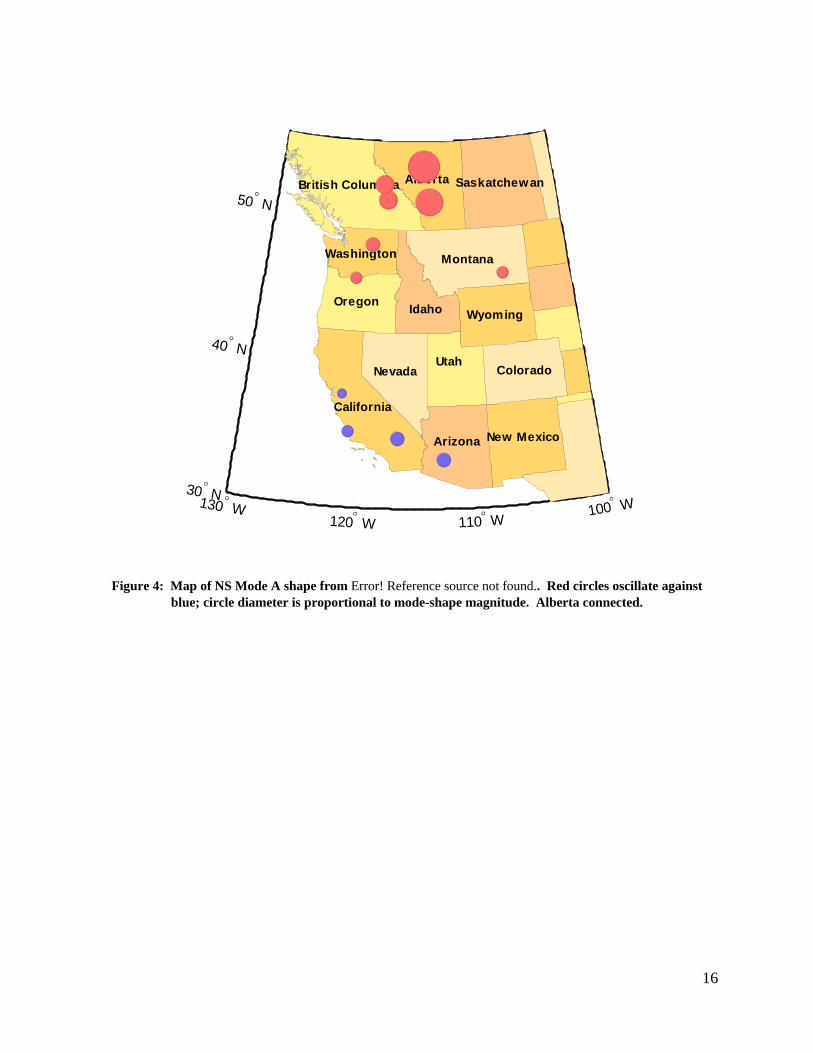
Figure 3 and Figure 4 show the mode shape for selected PMUs across the system. The reader is referred to [10] for a more detailed list of mode shapes. Note the two PMUs in Alberta (GN01 and LA01) have a much larger magnitude. GN01 is further north and is hypothesized to be near the center for the northern mass of the mode. The node or dividing line for the mode is north of Tesla and very close to Malin.

6

NS Mode B first showed up after Alberta interconnected to the system [5] and has a very widespread shape. Under normal operating conditions, the mode frequency varies from 0.34 Hz to 0.4 Hz. Recently during heaving loading, the damping is typically between 5% and 10%. It has the Alberta area swinging against BC and the northern US which in turn swings against the southern part of the US. The northern node or dividing line is just south of Langdon on the BC/Alberta intertie. The other node is typically south of Tesla and north of Diablo Canyon. The observability is much more widespread than NS Mode A in that no one location is dominant.

Figure 5 shows the mode estimates for a typical summer day. Note the diurnal variation in the mode frequency which is significantly more than NS Mode A. It is typical and expected that the mode frequency increases during the lighter loading time of the night. The mode damping slightly drops during the early morning hours. The faster variations in the damping are typical of random variations in the estimator algorithm. That is, when damping is high, the algorithm cannot exactly estimate the mode damping.

As with NS Mode A, the mode-shape estimates from the 2009 thru 2012 probe tests are very consistent. The Aug. 23, 2012 B tests represents the widest coverage mode-shape estimates to date. Figure 6 and Figure 7 show the NS Mode B shape for the same selected PMUs as shown previously for NS Mode A. Again, the reader is referred to [10] for more detailed mode-shape data. Note that the largest amplitude is located at GN01 (Genesee in Alberta). The amplitude at Langdon in Alberta is zero (too small to accurately estimate). This is likely because Langdon is at a node of the mode (i.e., a dividing line). Note that PV50 and DV01 in the southern part of the Western Interconnection swing in phase with GN01 in Alberta. Also, note the relatively large magnitude of the mode throughout the system. The other node or dividing line for the mode is just south of Tesla.

B. BC – Alberta tie disconnected

With Alberta disconnected, NS Modes A and B meld into a single north-south mode nominally near 0.32 Hz which again has a dividing line near the COI. This mode is typically lightly damped. This is likely the most lightly damped condition in the WECC system under normal operations.

The modal estimates for a typical Alberta disconnect are shown in Figure 8 Figure 9. The modes are estimated with an automated mode meter. The Alberta disconnect occurs just prior to the 1100 min. point. Note that Mode A disappears and Mode B suddenly drops in frequency and the damping slightly decreases. This is a typical response. The mode shape of the NS Mode B with Alberta disconnected is very similar to NS Mode B with Alberta except for the Alberta PMUs are not included.

7

Appendix A describes a BC-Alberta separation event that occurred on August 4, 2000 during high load, heavy transfer conditions. The event resulted in poorly dampened power oscillations in the Western Interconnection.

BC-Alberta tie was out of service for a prolonged period of time in August - September 2010. Several periods of low damping conditions for the NS mode were observed. This includes August 31, September 2, September 3, September 6, September 9, September 10, and September 11. The mode-meter estimates for August 31 are shown in Figure 10. Note the low damping near the 600 min. and 1300 min. points. The damping drops well below 5%. It is still unclear as to the cause of the low damping.

September 2 showed similar low damping conditions as seen on August 31. Also, wider coverage PMU data was available for September 2 allowing for mode shape analysis. Figure 11 shows the mode estimates. Note the low damping in the 230 min. to 310 min. range. Mode shape estimates for this range are shown in Table 1 and Figure 12. The mode shape is similar to NS Mode B with Alberta connected.

C. Weak BC – Alberta connection

On Sep. 13, 2012 during probing tests, Selkirk – Cranbrook 500-kV line was out of service, and Alberta remained connected via the lower voltage sub-transmission. This represents a very weak connection between BC and Alberta.

The NS mode A dropped to 0.18 Hz and the NS Mode B dropped to 0.32 Hz. Figure 13 thru Figure 16 show the mode shapes.

The observability of the NS Mode A in Figure 13 and Figure 14 is very much dominated by Alberta as indicated by the magnitude of the mode shape. The magnitude is more than 10 times larger in Alberta than any other area. This indicates that the mode has Alberta oscillating against the system more as a local mode.

The mode shape of the NS Mode B is shown in Figure 15 and Figure 16. It is very similar to the shape with Alberta fully connected.

D. Canada – US ties are open

NS Modes A and B also meld into a single north-south mode when the US disconnects from Canada. The mode’s frequency is typically higher than with an Alberta disconnect because of lost inertia of BC Canada. The mode damping is typically very small. No actual-system cases have been recorded; but, the condition has been studied via simulations. An example mode shape is shown in Figure 17 for transient simulation case. The mode shape was obtained from Prony analysis of the event. The mode frequency is at 0.400 Hz with unstable damping.

8

IV. EAST – WEST MODES

The EW Modes are not very well understood primarily because of a lack of historical PMU coverage. The 2013 tests are the first to have adequate coverage to begin to understand this mode. As of the writing of this paper, only one day of test data is available June 19, 2013. A few other non-test days from 2013 have also been analyzed with results consistent with the June 19 data. As the 2013 probing data becomes available, analyses focus on its properties. Building a knowledge base for this mode is a primary goal over the next couple years.

The EW Mode A shape estimates from the June 19, 2013 are shown in Figure 18 and Figure 19. This system is operating in a normal configuration with Alberta connected. The PMUs selected for analysis are not the same as used for NS modes above; but, the coverage is similar plus the PMUs at Jim Bridger (WY), Ault (CO), and Craig (CO). The frequency of the mode is 0.40 Hz.

The mode seems to have the eastern portion of the system centralized in Colorado oscillating against the system. The mode can also be observed in smaller amplitude in southern California.

The frequency of the EW Mode A and the NS Mode B are very close. This is shown in Figure 20. The red trace is the power spectrum of Genesee. It is dominated by NS Mode A at 0.24 Hz. The blue trace is the spectrum at John Day which is dominated by NS Mode B at 0.38 Hz. The green trace is the spectrum at Graig which is dominated by EW Mode A at 0.40 Hz.

V. BC – NORTHWEST MODE

The “BC” mode primarily has the BC area swinging against the Pacific NW US. It also ripples into the south with a lower magnitude. System studies show that the largest observability point is the Kemano power plant in BC. But, no PMU data has been available from Kemano to date. Certainly this mode is best controlled from generators in BC. More analysis will be done once Kemano data becomes available.

VI. MONTANA – NORTHWEST MODE

The “Montana” mode has Montana oscillating against the Pacific NW US. It is dominated by the Colstrip power plant. That is, basically it is a Colstrip local mode. But, because Colstrip is a large radial plant, the mode is low in frequency and ripples throughout the system.

The mode is normally well-dampened. However, outages of 500-kV lines, which often require bypass of series capacitors for SSR reasons, can result in a weak condition when the oscillation can become marginally dampened.

9

VII. RELATIVE OBSERVABILITY, ENERGY AND INTERACTIONS

The above discussion provides an overview of the individual modes. The goal of the following is to provide perspective on the observability of the NS modes relative to each other, and the interactions of the modes. Modal interaction is loosely defined to be a measure of modal energy exchange for a given mode between different areas of a system. A good way to view the interactions is via spectral plots. Future work will focus on quantifying interactions of the EW Mode A.

Figure 21 through Figure 26 show the estimated Power Spectral Densities (PSDs) of the FreqLFD signal at Genesee (Alberta), Mica (BC), Colstrip (MT), Chief Jo (WA), Big Eddy (OR), and Palo Verde (AZ) during the Aug. 23, 2012 probing tests. FreqLFD is the estimated frequency at a PMU calculated by taking the numerical derivative of the voltage phase angle. Each spectrum is shown for two data sets: “ambient” is when the PDCI probing is turned off; and “probing” for when the probing is turned on.

First, consider the ambient conditions. Each plot reveals considerable information about the relative observability of each mode. As an example, consider Figure 21. The large peak near 0.24 Hz tells us that the Genesee power plant has very large observability for the NS Mode A. The smaller peak near 0.35 Hz tells us that the Genesee swings considerably less at the NS Mode B compared to NS Mode A. Mode A tends to have larger observability than Mode B at Genesee, Mica, and Palo Verde. And, NS Mode B is more observable at Colstrip, Chief Jo, and Big Eddy.

Figure 27 thru Figure 31 show the spectrums of the MW flows on major interties. These plots provide information on the interaction between areas. Figure 28 specifically shows a time frequency plot over an entire typical day for Malin-Round Mountain 1. Surprisingly, NS Mode A tends to have higher energy in all the interaction spectrums than NS Mode B. Also, Colstrip MW has very low interaction energy at both NS modes (Figure 29); but, the FreqLFD at Colstrip in Figure 23 does show energy. This inconsistency is unexpected.

At this point, one should NOT conclude that the NS Mode A dominates a contingency response. In fact, the following discussion will argue that actually NS Mode B dominates the response to most contingencies. All one can conclude is that NS Mode A is highly observable in the AMBIENT interactions.

VIII. MODAL CONTROLLABILITY AND EXCITABILITY

Controllability analysis tells us the locations where control systems are effective to dampen a give mode. Excitability is related to controllability; it is a measure of contingencies that will excite a mode. Only limited controllability and excitability information can be extracted from actual-system measurements. Therefore, model studies are also needed.

10

While model studies are needed to fully comprehend controllability, the PDCI modulation tests do provide information on the ability of PDCI modulation to dampen oscillations. In each Figure 21 thru Figure 26 plot, the NS Mode A peak increases very little during probing. This tells us that the mode is NOT controllable from PDCI modulation. But, the NS Mode B energy near 0.35 Hz does significantly increase with probing. Therefore, this mode is very controllable from PDCI modulation. More detailed correlation analysis using coherency plots present in [10] further verifies this conclusion.

Current and future work is focusing on controllability analysis of the EW Mode A using the 2013 and future probing tests. Only recently have reliable PMU measurements become available from the east side of the system. Initial results are showing that this mode is not controllable from the PDCI. Also, future work will analyze simulation cases for controllability properties.

A. Modal Excitability

The PDCI probing spectrums in Figure 21 thru Figure 31 also provide evidence on the excitability of the modes. It is hypothesized that the NS Mode A is uncontrollable from any location except Alberta; from this, one can hypothesize that only contingencies involving the Alberta area will significantly excite the mode. Similarly, nearly all major contingencies excite NS Mode B because its controllability is much more widespread.

One can test the hypotheses on Prony analysis of actual-system events. When conducting Prony analysis, a good signal for estimating the modes is the Big Eddy – Malin FreqLFD Hz. The ambient spectrum of this signal is shown in Figure 32 for the Aug. 23, 2012 probe test. Note that both NS Modes are present in the signal. And, NS Mode A has a larger spectral peak than NS Mode B.

The first such event is a Chief Joseph brake pulse. Figure 33 shows the response of the Big Eddy – Malin signal, and Figure 34 shows the response of the Malin – Round M. 1 MW to a brake pulse on Sep. 15, 2011. The Prony results are shown in Table 2. Three modes were estimated in the Prony analysis – NS Modes A and B, and the BC Mode. These three modes make up the “Prony” response in Figure 33 and Figure 34. Table 2 shows the amplitudes of the modes estimated by the Prony analysis. Note that NS Mode B is approximately 3 times larger than NS Mode A for both signals. This is despite the fact that NS Mode A is much more observable in the ambient (as indicated by Figure 27, Figure 28, and Figure 32). This indicates that a Chief-Jo brake pulse excites the NS Mode B much more than NS Mode A.

A second contingency example is from a Palo Verde trip on July 4, 2012. The system response and Prony results for NS Modes A and B are shown in Figure 35, Figure 36, and Table 3. In this case, NS Mode B’s amplitude is more than double the amplitude of NS Mode A. The conclusion is that the Palo Verde event excites the NS Mode B much more than NS Mode A.

11

IX. CONCLUSIONS

This paper summarizes the modal properties of the dominant inter-area modes in the wNAPS. The primary focus has been on the most wide-spread and troublesome NS Mode A and the NS Mode B. Initial work on EW Mode A has also been presented. The properties are estimated based upon several years of actual-system data analyses and to a lesser extent, model-based analysis. NS modal properties include:

NS Mode A is typically near 0.25 Hz. Its damping is typically larger than NS Mode B with typical damping near 10% to 15%.

NS Mode B is typically in the 0.35 Hz to 0.4 Hz range with a damping of 5% to over 10%. The shape for NS Mode A has the northern half of the wNAPS swinging against the southern

half. By far, the most dominant observability point is the Alberta Canada area of the system. The node or dividing line is very close to Malin on the COI.

The shape for NS Mode B has the Alberta area swinging against BC and the northern US which in turn swings against the southern part of the US. The northern node or dividing line is just south of Langdon on the BC/Alberta intertie. The other node is typically south of Tesla and north if Diablo Canyon. The observability is much more widespread than NS Mode A in that no one location is dominant.

The controllability of NS Mode A is dominated by Alberta while the controllability of NS Mode B is very wide spread. Therefore, contingencies outside Alberta primarily excite NS Mode B.

The Alberta-BC intertie has the largest impact on the two modes. When Alberta disconnects, the two modes “melt” into one mode typically near 0.32 Hz. This mode typically is more lightly damped. The shape for this mode is very similar to NS Mode B excluding the Alberta area PMUs.

EW Mode A is very near in frequency to NS Mode B. Based upon one day of measurement, the mode seems to have the eastern portion of the system centralized in Colorado oscillating against the system. The mode can also be observed in smaller amplitude in southern California.

Current and future work will focus on continued monitoring of the NS modes as well as developing a better knowledge base for the EW modes.

X. ACKNOWLEDGMENT

The authors gratefully acknowledges the many years of collaboration with Dr. John Hauer, Mr. Bill Mittelstadt, Dr. Matt Donnelly, Dr. John Undrill, and Dr. John Pierre related to wNAPS dynamics and analysis methods.

12

XI. REFERENCES

[1] D. N. Kosterev, C. W. Taylor, and W. A. Mittelstadt, “Model Validation for the August 10, 1996 WSCC System Outage,” IEEE Trans. On Power Systems, vol. 14, no. 3, pp. 967-976, Aug. 1999.

[2] D. Trudnowski and J. Pierre, “Signal Processing Methods for Estimating Small-Signal Dynamic Properties from Measured Responses,” Chapter 1 of Inter-area Oscillations in Power Systems: A Nonlinear and Nonstationary Perspective, ISBN: 978-0-387-89529-1, Springer, 2009.

[3] G. Rogers, Power System Oscillations, Kluwer Academic Publishers, Boston, 2000. [4] F. L. Pagola, I. J. Perez-Arriaga, and G. C. Verghese, “On Sensitivities, Residues, and

Participations: Applications to Oscillatory Stability Analysis and Control,” IEEE Transactions on Power Systems, vol. 4, no. 1, pp. 278-285, Feb. 1989.

[5] J. F. Hauer, “Emergence of a New Swing Mode in the Western Power System,” IEEE Trans. On Power Apparatus and Systems, vol. PAS-100, no. 4, pp. 2037-2045, April 1981.

[6] J. F. Hauer, W. A. Mittelstadt, K. E. Martin, J. W. Burns, and Harry Lee in association with the Disturbance Monitoring Work Group of the Western Electricity Coordinating Council, “Integrated Dynamic Information for the Western Power System: WAMS Analysis in 2005,” Chapter 14 in the Power System Stability and Control volume of The Electric Power Engineering Handbook, 2nd Ed., L. L. Grigsby ed., CRC Press, Boca Raton, FL, 2007.

[7] D. Trudnowski and T. Ferryman, “Modal Baseline Analysis of the WECC System for the 2008/9 Operating Season,” Final Report to Pacific Northwest National Lab, Sep. 2010.

[8] D. Trudnowski, “Baseline Damping Estimates,” Appendix 4 of J. Undrill and D. Trudnowski, “Oscillation Damping Controls,” Year 1 report of BPA contract 37508, Sep. 2008.

[9] D. Trudnowski, “Transfer Function Results from the 2009 and 2011 PDCI Probing Tests,” Year 4 report of BPA contract 37508, Sep. 2011.

[10] D. Trudnowski, “2012 PDCI Probing Tests,” Year 6 report of BPA contract 37508, Sep. 2012.

[11] D. Trudnowski, “The MinniWECC System Model,” Appendix 2 of J. Undrill and D. Trudnowski, “Oscillation Damping Controls,” Year 1 report of BPA contract 37508, Sep. 2008.

[12] D. Trudnowski, “Modal and Controllability Analysis of the MinniWECC System Model,” Year 2 report of BPA contract 37508, Sep. 2009.

13

XII. FIGURES AND TABLES

14

Figure 1: Malin-Round Mountain #1 MW flow during the Aug. 10, 1996 breakup.

Figure 2: NS Mode A estimates for May 29, 2012. Plot starts at midnight GMT (5:00 pm PDT). Alberta strongly connected.

15

Figure 3: NS Mode A shape estimated during the Aug. 23, 2012 PDCI probing test B. GN01 = Genesee (Alberta), LA01 = Langdon (Alberta), REV1 = Revelstoke (BC), MCA1 = Mica (BC), COLS = Colstrip (MT), CHJ5 = Chief Jo (WA), BE50 = Big Eddy (OR), MALN (OR-CA), TSL5 (Mid CA), DCPP (So. CA), DV01 =

Devers (So. CA), PV50 = Palo Verde (AZ). Alberta connected.

0.5

1

1.5

30

210

60

240

90

270

120

300

150

330

180 0

GN01LA01

REV1

MCA1PV50

DV01

CHJ5

COLSDCPP

BE50

TSL5MALN

16

Figure 4: Map of NS Mode A shape from Error! Reference source not found.. Red circles oscillate against blue; circle diameter is proportional to mode-shape magnitude. Alberta connected.

130 W 120 W 110 W

100 W 30 N

40 N

Arizona

California

Colorado

Idaho

Montana

Nevada

New Mexico

Oregon

Utah

Washington

Wyoming

Alberta SaskatchewanBritish Columbia 50 N

17

Figure 5: NS Mode B estimates for May 29, 2012. Plot starts at midnight GMT (5:00 pm PDT), Alberta

strongly connected.

Figure 6: NS Mode B shape estimated during the Aug. 23, 2012 PDCI probing test B. GN01 = Genesee (Alberta), LA01 = Langdon (Alberta), REV1 = Revelstoke (BC), MCA1 = Mica (BC), COLS = Colstrip (MT), CHJ5 = Chief Jo (WA), BE50 = Big Eddy (OR), MALN (OR-CA), TSL5 (Mid CA), DCPP (So. CA), DV01 =

Devers (So. CA), PV50 = Palo Verde (AZ). Alberta strongly onnected.

0.5

1

1.5

30

210

60

240

90

270

120

300

150

330

180 0

GN01

CHJ5REV1

BE50

PV50

MALN

DV01

TSL5DCPP

LA01

18

Figure 7: Map of NS Mode B shape from Error! Reference source not found.. Red circles oscillate against blue; circle diameter is proportional to mode-shape magnitude. Alberta connected.

130 W 120 W 110 W

100 W 30 N

40 N

Arizona

California

Colorado

Idaho

Montana

Nevada

New Mexico

Oregon

Utah

Washington

Wyoming

Alberta SaskatchewanBritish Columbia 50 N

19

Figure 8: NS Mode A estimates for June 18, 2012. Plot starts at midnight GMT (5:00 pm PDT). Alberta

disconnects just prior to the 1100 min. point.

Figure 9: NS Mode B estimates for June 18, 2012. Plot starts at midnight GMT (5:00 pm PDT). Alberta

disconnects just prior to the 1100 min. point.

0 200 400 600 800 1000 1200 1400

0.2

0.25

Time (min.)

Mod

eF -

Hz

Mode 1

Estimate

0 200 400 600 800 1000 1200 14000

5

10

15

20

25

Mod

eD -

%

Time (min.)

20

Figure 10: NS Mode estimates for Aug. 31, 2010. Plot starts at midnight GMT (5:00 pm PDT). Alberta disconnected. Note low damping near 600 min. and 1300 min. points.

0 500 1000 15000.3

0.32

0.34

0.36

0.38

0.4F

req.

(H

z)

0 500 1000 15000

5

10

15

20

25

Dam

p (%

)

Time (min.)

21

Figure 11: NS Mode estimates for Sep. 2, 2010. Plot starts at 1200 min. point GMT. Alberta disconnected.

0 50 100 150 200 250 300 350 4000

5

10

15

20

25

Dam

ping

(%

)

Time (min.)

0 50 100 150 200 250 300 350 4000.25

0.3

0.35

Fre

q (H

z)

22

Table 1: Estimated mode shape at for Error! Reference source not found. mode for time = 230 min. to 310 min relative. Location Amplitude Angle (deg.)

GMS2 1.00 0

MCA1 0.97 8

REV1 0.91 4

SEL1 0.87 5

DMR1 0.87 ‐2

ING1 0.78 5

CST5 0.72 3

MPLV 0.53 8

COLS 0.53 6

CHJ5 0.52 2

BEL5 0.52 2

GAR5 0.50 1

ASHE 0.39 4

KEEL 0.38 10

MCN5 0.36 6

SLAT 0.32 10

BE50 0.32 11

JDAY 0.31 11

PV50 0.26 178

KY50 0.26 178

PP30 0.24 177

NV50 0.20 176

FC50 0.19 179

SUML 0.16 14

CPJK 0.13 16

MALN 0.12 16

23

Figure 12: Map of NS Mode shape from Table 1. Red circles oscillate against blue; circle diameter is proportional to mode-shape magnitude. Alberta disconnected.

130 W 120 W 110 W

100 W 30 N

40 N

50 N

Arizona

California

Colorado

Idaho

Montana

Nevada

New Mexico

Oregon

Utah

Washington

Wyoming

Alberta SaskatchewanBritish Columbia

24

Figure 13: NS Mode A shape estimated during the Sep. 13, 2012 PDCI probing test B. GN01 = Genesee (Alberta), LA01 = Langdon (Alberta), REV1 = Revelstoke (BC), MCA1 = Mica (BC), COLS = Colstrip (MT), CHJ5 = Chief Jo (WA), BE50 = Big Eddy (OR), MALN (CA-OR), TSL5 (Mid CA), DCPP (So. CA), DV01 = Devers (So. CA), PV50 = Palo Verde (AZ). NOTE: GN01, MCA1, DCPP, and TSL5 were not available for

analyses. Alberta weakly connected.

0.2

0.4

0.6

0.8

1

30

210

60

240

90

270

120

300

150

330

180 0

GN01LA01

REV1

MCA1PV50

DV01

CHJ5

COLSDCPP

BE50

TSL5MALN

25

Figure 14: Map of NS Mode A shape from Error! Reference source not found.. Red circles oscillate against blue; circle diameter is proportional to mode-shape magnitude. Alberta weakly connected.

130 W 120 W 110 W

100 W 30 N

40 N

50 N

Arizona

California

Colorado

Idaho

Montana

Nevada

New Mexico

Oregon

Utah

Washington

Wyoming

Alberta SaskatchewanBritish Columbia

26

Figure 15: NS Mode B shape estimated during the Sep. 13, 2012 PDCI probing test B. GN01 = Genesee (Alberta), LA01 = Langdon (Alberta), REV1 = Revelstoke (BC), MCA1 = Mica (BC), COLS = Colstrip (MT), CHJ5 = Chief Jo (WA), BE50 = Big Eddy (OR), MALN (OR-CA), TSL5 (Mid CA), DCPP (So. CA), DV01 = Devers (So. CA), PV50 = Palo Verde (AZ). NOTE: GN01, MCA1, DCPP, and TSL5 were not available for

analyses. Alberta weakly connected.

0.2

0.4

0.6

0.8

1

30

210

60

240

90

270

120

300

150

330

180 0

GN01MCA1

CHJ5

REV1COLS

BE50

PV50

MALNDV01

TSL5

DCPPLA01

27

Figure 16: Map of NS Mode B shape from Error! Reference source not found.. NOTE: GN01 was not available for analyses. Red circles oscillate against blue; circle diameter is proportional to mode-shape magnitude.

Alberta weakly connected.

130 W 120 W 110 W

100 W 30 N

40 N

Arizona

California

Colorado

Idaho

Montana

Nevada

New Mexico

Oregon

Utah

Washington

Wyoming

Alberta SaskatchewanBritish Columbia 50 N

28

Figure 17: Map of NS Mode shape obtained from Prony analysis of the transient simulation case XXX. Red circles oscillate against blue; circle diameter is proportional to mode-shape magnitude. Canada disconnected.

130 W 120 W 110 W

100 W 30 N

40 N

Arizona

California

Colorado

Idaho

Montana

Nevada

New Mexico

Oregon

Utah

Washington

Wyoming

Alberta SaskatchewanBritish Columbia 50 N

29

Figure 18: EW Mode A shape estimated during June 19, 2013. CUST = Custer (WA), MALN (OR-CA), GARR = Garrison (MT), JDAY = John Day (OR), BRID = Bridger (WY), FOUR = Four Corners, AULT

(CO), CRGC = Craig (CO), PV50 = Palo Verde (AZ), LUGO (So. CA), GN01 = Genesee (Alberta), COLS = Colstrip (MT), REV1 = Revelstoke (BC), WILS = Wiliston (BC), HASS = Hassayampa (AZ), SUND =

Sundance (Alberta).

1.68

1.26

0.84

0.42

00

30

60

90

120

150

180

210

240

270

300

330

CUST

MALN

GARR

JDAY

BRID

FOUR

AULT

CRGC

PV50

LUGO

GN01

COLS

REV1

WILS

HASS

SUND

30

Figure 19: Map of EW Mode A shape from Error! Reference source not found.. Red circles oscillate against blue; circle diameter is proportional to mode-shape magnitude.

130 W 120 W 110 W

100 W 30 N

40 N

50 N

Arizona

California

Colorado

Idaho

Montana

Nevada

New Mexico

Oregon

Utah

Washington

Wyoming

Alberta SaskatchewanBritish Columbia

31

Figure 20: Spectrum of three FreqLFD signals during June 19, 2013. GN01 = Genesee (Alberta), JDAY = John Day (OR), CRGC = Craig (CO).

Figure 21: Spectrum of Genesee FreqLFD during Aug. 23, 2012 probing test B.

0.1 0.2 0.3 0.4 0.5 0.6 0.7 0.8 0.9 1-80

-75

-70

-65

-60

-55

-50

-45

-40

Freq. (Hz)

PS

D (

dB)

GN01

JDAYCRGC

0.24 Hz

0.38 Hz

0.40 Hz

0 0.1 0.2 0.3 0.4 0.5 0.6 0.7 0.8 0.9 1-75

-70

-65

-60

-55

-50

-45

-40

-35

Freq. (Hz)

PS

D (

dB)

GN01 (Hz)

Ambient

Probing

32

Figure 22: Spectrum of Mica FreqLFD during Aug. 23, 2012 probing test B.

Figure 23: Spectrum of Colstrip FreqLFD during Aug. 23, 2012 probing test B.

Figure 24: Spectrum of Chief Jo FreqLFD during Aug. 23, 2012 probing test B.

0 0.1 0.2 0.3 0.4 0.5 0.6 0.7 0.8 0.9 1-85

-80

-75

-70

-65

-60

-55

-50

-45

Freq. (Hz)P

SD

(dB

)

MCA1 (Hz)

Ambient

Probing

0 0.1 0.2 0.3 0.4 0.5 0.6 0.7 0.8 0.9 1-85

-80

-75

-70

-65

-60

-55

-50

-45

Freq. (Hz)

PS

D (

dB)

COLS (Hz)

Ambient

Probing

0 0.1 0.2 0.3 0.4 0.5 0.6 0.7 0.8 0.9 1-85

-80

-75

-70

-65

-60

-55

-50

-45

Freq. (Hz)

PS

D (

dB)

CHJ5 (Hz)

Ambient

Probing

33

Figure 25: Spectrum of Big Eddy FreqLFD during Aug. 23, 2012 probing test B.

Figure 26: Spectrum of Palo Verde FreqLFD during Aug. 23, 2012 probing test B.

Figure 27: Spectrum of Malin-Round M. 1 MW during Aug. 23, 2012 probing test B.

0 0.1 0.2 0.3 0.4 0.5 0.6 0.7 0.8 0.9 1-85

-80

-75

-70

-65

-60

-55

-50

-45

Freq. (Hz)P

SD

(dB

)

BE50 (Hz)

Ambient

Probing

0 0.1 0.2 0.3 0.4 0.5 0.6 0.7 0.8 0.9 1-90

-85

-80

-75

-70

-65

-60

-55

-50

Freq. (Hz)

PS

D (

dB)

PV50 (Hz)

Ambient

Probing

0 0.1 0.2 0.3 0.4 0.5 0.6 0.7 0.8 0.9 1-15

-10

-5

0

5

10

15

20

25

Freq. (Hz)

PS

D (

dB)

MALN Round Mountain 1 C MW

Ambient

Probing

34

Figure 28: Waterfall Spectrum of Malin-Round M. 1 MW during June 1, 2008.

Figure 29: Spectrum of Colstrip MW during Aug. 23, 2012 probing test B.

Figure 30: Spectrum of Bell-Boundary MW during Aug. 23, 2012 probing test B.

0 0.1 0.2 0.3 0.4 0.5 0.6 0.7 0.8 0.9 1-20

-15

-10

-5

0

5

10

15

20

Freq. (Hz)

PS

D (

dB)

COLS Broadview 1 & 2 Cu MW

Ambient

Probing

0 0.1 0.2 0.3 0.4 0.5 0.6 0.7 0.8 0.9 1-25

-20

-15

-10

-5

0

5

10

15

Freq. (Hz)

PS

D (

dB)

BEL2 Boundary 1 current MW

Ambient

Probing

35

Figure 31: Spectrum of Alberta-BC MW during Aug. 23, 2012 probing test B.

Figure 32: Spectrum of Big Eddy - Malin FreqLFD during Aug. 23, 2012 probing test B.

Figure 33: Prony fit to Sep. 15, 2011 brake pulse A3, Big Eddy - Malin FreqLFD Hz.

0 0.1 0.2 0.3 0.4 0.5 0.6 0.7 0.8 0.9 1-5

0

5

10

15

20

25

30

35

Freq. (Hz)P

SD

(dB

)

LA01 1201L MW

Ambient

Probing

0 0.1 0.2 0.3 0.4 0.5 0.6 0.7 0.8 0.9 1-95

-90

-85

-80

-75

-70

-65

-60

-55

Freq. (Hz)

PS

D (

dB)

BE50-MALN (Hz)

Ambient

Probing

0 2 4 6 8 10 12 14 16 18 20-0.015

-0.01

-0.005

0

0.005

0.01

0.015

Time (sec.)

BE

50-M

ALN

Hz

Brake A3

Actual

Prony

36

Figure 34: Prony fit to Sep. 15, 2011 brake pulse A3, Malin-RM 1 MW.

Table 2: Modal amplitudes (or residues) from Figure 33 and Figure 34. NS Mode A NS Mode B BC Mode

0.261 Hz, 12.5%D 0.391 Hz, 11.2%D 0.657 Hz, 11.1 %D

BE50‐

MALN (Hz) 0.00151 0.00563 0.00365

Malin‐RM 1 

MW 22.3 62.6 21.2

Amplitude

Figure 35: Prony fit to July 4, 2012 Palo Verde event, Big Eddy - Malin FreqLFD Hz.

0 2 4 6 8 10 12 14 16 18 20850

900

950

1000

1050

1100

Time (sec.)

Mal

in-R

M 1

MW

Brake A3

Actual

Prony

0 10 20 30 40 50 60-0.01

-0.008

-0.006

-0.004

-0.002

0

0.002

0.004

0.006

0.008

0.01

Time (sec.)

BE

50-M

ALN

Hz

Actual

Prony

37

Figure 36: Prony fit to July 4, 2012 Palo Verde event, Malin-RM 1 MW.

Table 3: Modal amplitudes (or residues) from Figure 35 and Figure 36. NS Mode A NS Mode B

0.257 Hz, 10.5%D 0.386 Hz, 8.0%D

BE50‐MALN 

(Hz)0.0131 0.0586

Malin‐RM 1 

MW331 756

Amplitude

0 10 20 30 40 50 601250

1300

1350

1400

1450

1500

1550

1600

1650

Time (sec.)

Mal

in-R

M 1

MW

Actual

Prony

38

XIII. APPENDIX A: AUGUST 4, 2000 DISTURBANCE EVENT

High temperatures were across the Western Interconnection on August 4, 2000, and loads were close to their peak levels in most areas. The flows were moderate-high from North to South: Canada – Northwest: 2700 MW North-of-Hanford: 3570 MW (3700 MW limit) North-of-John Day cutplane: 7695 MW (7800 MW limit) Pacific HVDC Intertie: 2418 MW California – Oregon Intertie: 3097 MW Reno-Alturas: 247 MW Summer Lake – Midpoint: 72 MW Northern – Southern California: 2165 MW Large North-South phase angles correspond with the high North-South flows: Grand Coulee – John Day angle: 37.5 deg Grand Coulee – Malin angle: 56 deg Grand Coulee – Vincent angle: 78 deg Grand Coulee – Devers angle: 92 deg At 12:56 PM Pacific Time, a high-impedance single-phase to ground fault occurred on the Selkirk – Cranbrook 500-kV line. Line clearing initiated a BC Hydro RAS action – opened the ties between BC and Alberta: Cranbrook – Langdon 500 kV line and Natal 138kV tie. At that time, power flow from BC to Alberta was approximately 400 MW. The Alberta separation rerouted power south and initiated power oscillations in the system. Figure 1 shows the power oscillations at (a) Malin 500-kV bus voltage, (b) Custer 500-kV bus voltage, (c) BC – NW tie power, (d) California-Oregon Intertie power. It took longer than 60 seconds for the oscillation to dampen out [A1] [A1] Model Validation and Analysis of WSCC System Oscillations following Alberta Separation on August 4, 2000, report prepared by BPA and BC Hydro

39

Figure A-1: recorded oscillations on August 4, 2000

0 10 20 30 40 50 602400

2600

2800

3000

3200P

ower

[M

W]

(a) Canada - Northwest Power

0 10 20 30 40 50 603000

3200

3400

3600

Pow

er [

MW

]

(b) California - Oregon Intertie Power

0 10 20 30 40 50 60515

520

525

530

Vol

tage

[kV

]

(c) Custer 500-kV Bus Voltage

0 10 20 30 40 50 60525

530

535

540

545

Time [sec]

Vol

tage

[kV

]

(d) Malin 500-kV Bus Voltage

40

XIV. APPENDIX B: THEORETICAL BACK GROUND

A. Modal Analysis Terms

Electromechanical modes are defined by the following terms. For more detailed information on the topic, we recommend [3].

Mode frequency: The frequency at which a given mode oscillates (typically in Hz). Mode damping: A measure of how long it takes for a given mode to dissipate in a transient.

Typically measured in %D where %D = 100*(damping ratio). Note, 1/(damping ratio) ≅ the number of cycles of an oscillation before the oscillation completely dissipates. A damping of 10% or more is considered high and very safe. A damping below 5% is considered low. And, a damping below 3% is very low.

Observability: The content of a given mode in a given measured signal. Mode Shape: A measure of the observability of a given mode. Mode shape is a complex

number and is associated with a given mode and system state (e.g., generator speed). The amplitude of the shape is a measure of the magnitude of the state variable in the modal oscillations. The angle of the shape is a measure of the phase of the state variable in the modal oscillations.

Controllability: The extent to which a given mode can be damped from control of a given actuator at a given location in the grid.

Participation Factor: A measure of controllability of a given mode at a given location (typically a generator). The participation factor is a direct measure of how much damping a PSS unit at a given generator can dampen an oscillation of a give mode.

Modal Interaction: Loosely defined as a measure of modal energy exchange between different areas of a system. For example, if two areas swing against each other at a given mode, modal energy is exchanged through one or more transmission lines. Interaction is a measure of modal energy being exchanged on a given line.

Modal Excitability: Loosely defined to be a measure of how much a given contingency excites an oscillation containing a given mode

B. Theory and Definition of Modal Terms

Consistent with power-system dynamic theory [3], we assume that a power system can be linearized about an operating point. The underlying assumption is that small motions of the power system can be described by a set of ordinary differential equations of the form

tuDtCxty

tuBtxAtx

E

E

(1)

41

where vector x contains all system states including generator angles and speeds, and t is time. Note that variables with an underline are vectors. System inputs are represented by the exogenous input vector uE. Measurable signals are represented by y.

Define the eigen-terms for the system in (1) as

iii uuA (2a)

iii vAv (2b)

1ii uv (2c)

0ji uv , for ji (2d)

where

A = state matrix,

ui = nx1 ith right eigenvector,

vi = 1xn ith left eigenvector, and

λi = ith eigenvalue.

Define

nuuU 1 (3a)

nv

v

V 1

(3b)

and note that

IVUUV (3c)

where I is the nxn identity matrix.

Modal properties are described by an eigenvalues and eigenvectors. A given mode oscillates at the imaginary part of the eigenvalue (rad/s) and the damping is defined by the eigenvalue’s damping ratio (%). Mode shape is described by the right eigenvector of the A matrix corresponding to a generators speed variable. Let ui,k = the kth element of the ith right eigenvector; ui,k provides the critical information on the ith mode (eigenvalue) in the kth state. The amplitude of ui,k is the weight for the magnitude of mode i in state xk. It is a direct measure of the observability of the mode in the state. The angle of ui,k provides the relative phasing of

42

mode i in state xk. By comparing the kiu , for a common generator state (such as the speed), one

can determine phasing of the oscillation for the ith mode. As such, ui has been termed the “mode shape.” For the results presented in this paper, all mode shapes are normalized to the largest term in the vector ui.

Although the right eigenvector provides critical information on the observability of a mode, it does not provide information on the controllability of the mode. Controllability is best described by the participation factor. Participation factor is the sensitivity of a mode to a given state variable and is calculated from the left and right eigenvectors. It is common to select a generator’s speed state.

The participation factor for eigenvalue (mode) i and state k is defined to be

ikikik uvp (4)

where vik is the kth element of vi, and uik is the kth element of ui. The participation factor can be interpreted using the feedback system in Figure B-1. As shown in [4], the sensitivity of the eigenvalue to the feedback gain is then

iki p

dK

d

(5)

Equation (5) is the foundation for determining which generators with PSS units will dampen a give mode the most. For example, assume xk is the speed state of a generator. Basically, the equation tells us that the vector of departure in the root locus is equal to the participation factor when controlling the speed state of a generator through the torque on the shaft. In this sense, it is a direct measure of the controllability for the generator associated with state k on mode i. The magnitude of pik is the rate at which the locus leaves the open-loop pole and the angle of pik is the angle of departure. Effectively, the participation factor is a measure as to how well control on a given generator can relatively dampen a given mode.

PowerSystem xkkx

K

+

- Gen speedGen acel.

Figure B-1: Feedback system perspective of participation factors.

The participation factors are typically normalized by the inertia constant (H) of the machine scaled to a common system base.

43

Electromechanical modes are typically classified as “local” or “inter-area.” Local modes have a single generator or power-plant oscillating against the system. An inter-area mode has several generators swinging in phase against several other generators.

C. A simple example

As a simple example, consider the system in Figure B-2. The system has three electromechanical modes described in Table B-1. Mode 2 is a local mode that has generators 1 and 2 swinging against each other. Similarly, Modes 3 is a local mode that has generators 3 and 4 swinging against each other.

Mode 1 is an “inter-area” mode. The mode shape is shown in Table B-2. The table clearly indicates that for mode 1, generators 1 and 2 swing together against generators 3 and 4. Also, for a given disturbance, generators 1 and 2 will have approximately double the amplitude of swing at the 0.51-Hz mode.

This is demonstrated with the simple transient simulation shown Figure B-3. Note at the lower frequency movement in the system’s response at 0.51 Hz. Generators 1 and 2 move together while generators 3 and 4 swing together 180 degrees out of phase from generators 1 and 2. Also note that generators 1 and 2 have roughly double the amplitude of movement at the 0.51 Hz mode.

1 3

4 2

1 5

2

6

4

7 3 11 9 10 8

Figure B-2: Simple 4-machine example system.

Table B-1: 4-machine modes.

ModeFrequency

(Hz)Damping

(%)1 0.51 7.80

2 1.19 3.40

3 1.22 3.30

44

Table B-2: 0.51-Hz 4-machine mode shape.

GenAngle(u i,k ) (degrees)

Amplitude |u i,k |

3 -180 1.00

4 -180 0.84

1 0 0.42

2 0 0.31

Figure B-3: Transient simulation for 4-machine system.

0 2 4 6 8 1059.9

59.95

60

60.05

60.1

60.15

60.2

Time (sec)

Spe

ed

(Hz)

Gen 1Gen 2Gen 3Gen 4