doctorat de l'universitÉ de toulouse - irit · to check the scalability of the integrated rdc...
TRANSCRIPT

En vue de l'obtention du
DOCTORAT DE L'UNIVERSITÉ DE TOULOUSEDélivré par :
Institut National Polytechnique de Toulouse (INP Toulouse)Discipline ou spécialité :
Réseaux, Télécommunications, Systèmes et Architecture
Présentée et soutenue par :M. HAMDI AYED
le jeudi 27 novembre 2014
Titre :
Unité de recherche :
Ecole doctorale :
ANALYSE ET OPTIMISATION DES RESEAUX AVIONIQUESHETEROGENES
Mathématiques, Informatique, Télécommunications de Toulouse (MITT)
Institut de Recherche en Informatique de Toulouse (I.R.I.T.)Directeur(s) de Thèse :M. CHRISTIAN FRABOUL
M. AHLEM MIFDAOUI
Rapporteurs :M. LAURENT GEORGE, UNIVERSITE DE MARNE LA VALLEE
M. YE-QIONG SONG, UNIVERSITE DE LORRAINE
Membre(s) du jury :1 M. LAURENT GEORGE, UNIVERSITE DE MARNE LA VALLEE, Président2 M. AHLEM MIFDAOUI, ISAE TOULOUSE, Membre2 M. CHRISTIAN FRABOUL, INP TOULOUSE, Membre2 M. JUAN LOPEZ, AIRBUS FRANCE, Membre2 M. LUIS ALMEIDA, UNIVERSIDADE DO PORTO PORTUGAL, Membre


Acknowledgments
I would like to express my sincere gratitude to my supervisor Christian Fraboul and
Co-supervisor Ahlem Mifdaoui for their constant support, guidance and patience during
my research. I thank them for their precious advice, availability and kindness they have
shown during my thesis. Without their help and support in the difficult moments this
thesis would not have been possible.
I am thankful for Ye-Qiong Song and Laurent George for accepting to be my thesis
referees. I am also very honored to count them among the members of the jury of my
thesis as well as Luis Almeida and Juan Lopez.
I would like to thank Sylvie Eichen for her precious help in administrative tasks.
I thank all the people that i worked or interacted with at the Department of Computer
Science, Mathematics and Automatics (DMIA) of the ISAE (Jolimont site). In particular,
I am grateful to Emmanuel Lochin, Fabrice Frances, Jerome Lacan, Patrick Senac, Tan-
guy Perennou and Pierre de-Saqui-Sannes for the many useful discussions and precious
advice. I thank Thomas, Remi, Hugo, Anh-Dung, Nicolas, Victor, Leo, Jonathan, Tuan,
Khanh, Viet, Rami, Karine, Ahmed and everyone in the DMIA department for providing
me a friendly working environment.
Finally, I thank my parents and all my family for their encouragement and support.
iii

iv

Abstract
The complexity of avionic communication architecture is increasing due to the grow-
ing number of interconnected end-systems and the expansion of exchanged data. To
be effective in meeting the emerging requirements in terms of bandwidth, latency and
modularity, the current avionic communication architecture consists of an Avionics Full
DupleX Switched Ethernet (AFDX) network to interconnect the critical end-systems and
some Input/ Output (I/O) data buses (e.g., Controller Area Network (CAN) bus) for sen-
sors and actuators. Clusters are then interconnected via specific devices, called Remote
Data Concentrators (RDCs), standardized as ARINC 655. RDC devices are modular
gateways distributed throughout the aircraft to handle heterogeneity between the AFDX
backbone and I/O data buses. Although RDC devices enhance avionics modularity and
reduce maintenance efforts, they become one of the major challenges in the design pro-
cess of such multi-cluster avionic architectures. The existing implementations of RDC
are usually based on direct frames translation and do not consider resource savings issue.
Resource utilization efficiency is important for avionic applications to guarantee easy in-
cremental design, and enhance margins for future avionic functions additions. Therefore,
the design of an optimized RDC device integrating resource saving mechanisms becomes
a necessity to enhance the scalability and performances of avionic applications. In this
context, the main objective of this thesis is to design and validate an enhanced RDC
device offering an efficient bandwidth utilization, considered as a main resource to save,
while meeting real-time constraints.
To achieve this aim, first, we design an enhanced CAN-AFDX RDC device compliant
with the ARINC 655 specifications. The main elementary functions integrated into the
proposed RDC are: (i) frame packing applied on upstream flows, i.e., flows generated
by sensors and destined to the AFDX, to minimize communication overheads, and con-
sequently bandwidth utilization; (ii) hierarchical traffic shaping applied on downstream
flows, i.e., flows generated by AFDX sources and destined to actuators, to reduce inter-
ferences on CAN, and thus to enhance communication efficiency. Moreover, our proposed
RDC may connect multiple I/O CAN buses using a partitioning process to guarantee the
isolation between different criticality levels.

Second, to analyze the effects of our proposed RDC on the system’s performance, we
detail the modeling of the CAN-AFDX architecture, and especially the RDC device and
its implemented functions. Afterwards, we conduct timing analysis to compute end-to-
end delay bounds and to verify real-time constraints. Preliminary performance analysis of
our proposed RDC device through simple examples shows the efficiency of frame packing
and traffic shaping processes to enhance resource savings in terms of AFDX bandwidth
utilization.
Many RDC configurations can meet the system requirements while enhancing resource
savings. Hence, we proceed to tuning of our RDC parameters to maximize as much as
possible resource savings, and consequently to minimize the AFDX bandwidth utilization
while meeting the system constraints. However, this RDC tuning problem turned to be
a NP-hard problem, and adequate heuristic methods are introduced to find the accurate
RDC parameters. Preliminary performance evaluation of our optimized RDC device has
been performed, and obtained results show significant enhancements in terms of band-
width utilization reduction, with reference to the currently used RDC device.
Finally, the performances of the proposed RDC device are validated through a real-
istic CAN-AFDX avionics architecture. Different I/O CAN loads have been considered
to check the scalability of the integrated RDC functions, i.e., frame packing and traffic
shaping. The obtained results confirm our first conclusions and highlight the ability of
our proposed RDC device to maximize resource savings, while meeting the real-time con-
straints. For instance, the optimized RDC device offers a bandwidth utilization reduction
of more than 40% compared to current RDC device.
Keywords: Multi-cluster avionics networks, AFDX, CAN, RDC design, Timing analysis,
performance optimization, Validation

List of Publications
[RTSS2011] Hamdi Ayed, Ahlem Mifdaoui and Christian Fraboul. Gateway Optimiza-
tion for an Heterogeneous Avionics Network AFDX-CAN. In: WIP session of the
32nd IEEE Real-Time Systems Symposium (RTSS), 29 Nov - 02 Dec 2011, Vienna,
Austria.
[ETFA2012] Hamdi Ayed, Ahlem Mifdaoui and Christian Fraboul. Frame Packing
Strategy within Gateways for Multi-cluster Avionics Embedded Networks. In: 17th
Emerging Technologies & Factory Automation (ETFA), Krakow, 17-21 Sept. 2012.
[ECRTS2013] Hamdi Ayed, Ahlem Mifdaoui and Christian Fraboul. Interconnection
Optimization for Multi-Cluster Avionics Networks. In: 5th Euromicro Conference
on Real-Time Systems (ECRTS), 2013, 9-12 July 2013.
[SIES2014] Hamdi Ayed, Ahlem Mifdaoui and Christian Fraboul. Hierarchical Traffic
Shaping and Frame Packing to Reduce Bandwidth Utilization in the AFDX. In: 9th
IEEE International Symposium on Industrial Embedded Systems (SIES), Pisa, 18-
20 June.
[ESL2014] Hamdi Ayed, Ahlem Mifdaoui and Christian Fraboul. Enhanced RDC Device
to Maximize Resource Savings for Avionics Networks. In: IEEE Embedded Systems
Letters (under submission).
vii

List of Publications
viii

Contents
List of Publications vii
List of Figures xiii
List of Tables xvii
Introduction
Context and Motivation . . . . . . . . . . . . . . . . . . . . . . . . . . . . . . . 1
Original Contributions . . . . . . . . . . . . . . . . . . . . . . . . . . . . . . . . 3
Thesis Outline . . . . . . . . . . . . . . . . . . . . . . . . . . . . . . . . . . . . 4
1 Background and Problem Statement
1.1 Progress of Avionic Communication Architecture and Main Challenges . . 7
1.1.1 History of Avionic Architecture . . . . . . . . . . . . . . . . . . . . 8
1.1.2 Appearance of Multi-cluster Avionic Networks . . . . . . . . . . . . 9
1.2 Description of Network Standards . . . . . . . . . . . . . . . . . . . . . . . 13
1.2.1 ARINC 664: Backbone Network . . . . . . . . . . . . . . . . . . . . 13
1.2.2 Sensors/Actuators Networks . . . . . . . . . . . . . . . . . . . . . . 17
1.3 Description of RDC Standard: ARINC 655 . . . . . . . . . . . . . . . . . . 22
1.3.1 RDC Requirements . . . . . . . . . . . . . . . . . . . . . . . . . . . 22
1.3.2 Functional Specifications . . . . . . . . . . . . . . . . . . . . . . . . 24
1.3.3 Architectural Specifications . . . . . . . . . . . . . . . . . . . . . . 25
1.4 Design Opportunities for Multi-Cluster Avionic Networks . . . . . . . . . . 26
1.5 Conclusion . . . . . . . . . . . . . . . . . . . . . . . . . . . . . . . . . . . . 28
2 Related Work: Performance Optimization for Multi-Cluster Networks
ix

Contents
2.1 Optimizing Traffic-Source Mapping . . . . . . . . . . . . . . . . . . . . . . 29
2.1.1 Avionics End-Systems . . . . . . . . . . . . . . . . . . . . . . . . . 30
2.1.2 Automotive End-Systems . . . . . . . . . . . . . . . . . . . . . . . 32
2.2 Optimizing Communication Network Performance . . . . . . . . . . . . . . 33
2.2.1 Work on the AFDX Network . . . . . . . . . . . . . . . . . . . . . . 34
2.2.2 Work on Sensors/Actuators Networks . . . . . . . . . . . . . . . . . 38
2.3 Optimizing Interconnection Devices . . . . . . . . . . . . . . . . . . . . . . 41
2.3.1 CAN-Ethernet Bridge . . . . . . . . . . . . . . . . . . . . . . . . . 41
2.3.2 CAN-FlexRay Gateway . . . . . . . . . . . . . . . . . . . . . . . . 42
2.3.3 ARINC 429-AFDX Gateway . . . . . . . . . . . . . . . . . . . . . . 45
2.4 Need for Optimized CAN-AFDX Gateway . . . . . . . . . . . . . . . . . . 46
2.5 Conclusion . . . . . . . . . . . . . . . . . . . . . . . . . . . . . . . . . . . . 48
3 Design of an Enhanced CAN-AFDX RDC
3.1 Current RDC Device . . . . . . . . . . . . . . . . . . . . . . . . . . . . . . 51
3.2 Enhanced RDC Functional Overview . . . . . . . . . . . . . . . . . . . . . 54
3.3 Frame Packing Strategies . . . . . . . . . . . . . . . . . . . . . . . . . . . . 57
3.3.1 Related Work . . . . . . . . . . . . . . . . . . . . . . . . . . . . . . 57
3.3.2 Dynamic Strategy: FWT . . . . . . . . . . . . . . . . . . . . . . . . 59
3.3.3 Static Strategy: MSP . . . . . . . . . . . . . . . . . . . . . . . . . . 60
3.4 Data Mapping & Formatting . . . . . . . . . . . . . . . . . . . . . . . . . . 60
3.4.1 Data Mapping . . . . . . . . . . . . . . . . . . . . . . . . . . . . . . 60
3.4.2 Frame Formatting . . . . . . . . . . . . . . . . . . . . . . . . . . . . 61
3.5 Traffic Shaping Mechanism . . . . . . . . . . . . . . . . . . . . . . . . . . . 64
3.5.1 Related Work . . . . . . . . . . . . . . . . . . . . . . . . . . . . . . 64
3.5.2 HTS Algorithm . . . . . . . . . . . . . . . . . . . . . . . . . . . . . 66
3.6 Conclusion . . . . . . . . . . . . . . . . . . . . . . . . . . . . . . . . . . . . 67
4 Modeling and Timing Analysis of the Enhanced RDC
4.1 CAN-AFDX RDC Modeling . . . . . . . . . . . . . . . . . . . . . . . . . . 69
4.1.1 Frame Packing Strategies Modeling . . . . . . . . . . . . . . . . . . 71
4.1.2 HTS Mechanism Modeling . . . . . . . . . . . . . . . . . . . . . . . 75
4.2 Timing Analysis . . . . . . . . . . . . . . . . . . . . . . . . . . . . . . . . . 76
4.2.1 Sufficient Schedulability Test . . . . . . . . . . . . . . . . . . . . . . 76
4.2.2 Timing Analysis for Upstream Flows . . . . . . . . . . . . . . . . . 78
x

4.2.3 Timing Analysis for Downstream Flows . . . . . . . . . . . . . . . . 84
4.3 Preliminary Performance Analysis . . . . . . . . . . . . . . . . . . . . . . . 87
4.3.1 Considered Test Cases . . . . . . . . . . . . . . . . . . . . . . . . . 87
4.3.2 Impact of Frame Packing Strategy . . . . . . . . . . . . . . . . . . 89
4.3.3 Impact of HTS Mechanism . . . . . . . . . . . . . . . . . . . . . . . 93
4.4 Conclusion . . . . . . . . . . . . . . . . . . . . . . . . . . . . . . . . . . . . 95
5 Performance Optimization of the Enhanced RDC
5.1 Problem Formulation . . . . . . . . . . . . . . . . . . . . . . . . . . . . . . 97
5.2 Optimization Process under FWT Strategy . . . . . . . . . . . . . . . . . . 99
5.3 Optimization Process under MSP Strategy . . . . . . . . . . . . . . . . . . 102
5.3.1 Bandwidth Best Fit Decreasing Heuristic . . . . . . . . . . . . . . . 104
5.3.2 Branch & Bound Algorithm . . . . . . . . . . . . . . . . . . . . . . 106
5.4 Optimization process under HTS Mechanism . . . . . . . . . . . . . . . . . 110
5.4.1 Heuristic Approach . . . . . . . . . . . . . . . . . . . . . . . . . . . 110
5.4.2 Example . . . . . . . . . . . . . . . . . . . . . . . . . . . . . . . . . 111
5.5 Preliminary Performances Analysis . . . . . . . . . . . . . . . . . . . . . . 112
5.5.1 Results under Optimized FWT Strategy . . . . . . . . . . . . . . . 113
5.5.2 Results under Optimized MSP Strategy . . . . . . . . . . . . . . . . 114
5.5.3 Results under Optimized HTS Mechanism . . . . . . . . . . . . . . 116
5.6 Conclusion . . . . . . . . . . . . . . . . . . . . . . . . . . . . . . . . . . . . 117
6 Avionics Case Study
6.1 Description . . . . . . . . . . . . . . . . . . . . . . . . . . . . . . . . . . . 119
6.1.1 CAN-AFDX Architecture . . . . . . . . . . . . . . . . . . . . . . . 119
6.1.2 Communication Traffic . . . . . . . . . . . . . . . . . . . . . . . . . 120
6.1.3 Test Scenarios . . . . . . . . . . . . . . . . . . . . . . . . . . . . . . 122
6.2 Benefits of Frame Packing Strategies . . . . . . . . . . . . . . . . . . . . . 122
6.2.1 Under FWT . . . . . . . . . . . . . . . . . . . . . . . . . . . . . . . 123
6.2.2 Under MSP . . . . . . . . . . . . . . . . . . . . . . . . . . . . . . . 124
6.2.3 Comparative Analysis and Conclusion . . . . . . . . . . . . . . . . 124
6.3 Benefits of HTS Mechanism . . . . . . . . . . . . . . . . . . . . . . . . . . 125
6.3.1 Impact of I/O CAN Bus Sharing on Frame Packing . . . . . . . . . 125
6.3.2 On the Effects of HTS Mechanism . . . . . . . . . . . . . . . . . . . 128
6.4 Conclusion . . . . . . . . . . . . . . . . . . . . . . . . . . . . . . . . . . . . 129
xi

Contents
Conclusions and Prospectives
Conclusions . . . . . . . . . . . . . . . . . . . . . . . . . . . . . . . . . . . . . . 131
Prospectives . . . . . . . . . . . . . . . . . . . . . . . . . . . . . . . . . . . . . . 134
A Network Calculus Overview
A.1 Network Calculus Theory . . . . . . . . . . . . . . . . . . . . . . . . . . . 137
A.1.1 Cumulative Functions . . . . . . . . . . . . . . . . . . . . . . . . . 137
A.1.2 Arrival Curve . . . . . . . . . . . . . . . . . . . . . . . . . . . . . . 138
A.1.3 Service Curve . . . . . . . . . . . . . . . . . . . . . . . . . . . . . . 140
A.1.4 Network Calculus Bounds . . . . . . . . . . . . . . . . . . . . . . . 141
A.1.5 Concatenation and Blind Multiplexing . . . . . . . . . . . . . . . . 142
A.1.6 Application to AFDX . . . . . . . . . . . . . . . . . . . . . . . . . . 142
A.2 WoPANets Performance Analysis Tool . . . . . . . . . . . . . . . . . . . . 143
A.2.1 WoPANets Features and Structure . . . . . . . . . . . . . . . . . . 144
A.2.2 Propagation Analysis Algorithm . . . . . . . . . . . . . . . . . . . . 145
A.2.3 Illustrative Example . . . . . . . . . . . . . . . . . . . . . . . . . . 147
A.2.4 Obtained Results . . . . . . . . . . . . . . . . . . . . . . . . . . . . 148
B Generalization for TTCAN bus
B.1 TTCAN Description . . . . . . . . . . . . . . . . . . . . . . . . . . . . . . 151
B.2 TTCAN-AFDX RDC design . . . . . . . . . . . . . . . . . . . . . . . . . . 154
B.2.1 FWT strategy . . . . . . . . . . . . . . . . . . . . . . . . . . . . . . 154
B.2.2 MSP strategy . . . . . . . . . . . . . . . . . . . . . . . . . . . . . . 156
B.3 Timing Analysis . . . . . . . . . . . . . . . . . . . . . . . . . . . . . . . . . 157
B.3.1 Timing Analysis for RDC . . . . . . . . . . . . . . . . . . . . . . . 158
B.3.2 Timing Analysis on TTCAN . . . . . . . . . . . . . . . . . . . . . . 159
B.3.3 Illustrative Example . . . . . . . . . . . . . . . . . . . . . . . . . . 159
Bibliography 163
xii

List of Figures
1.1 Avionic network architecture: dedicated I/O networks . . . . . . . . . . . . 11
1.2 Centralized avionic architecture . . . . . . . . . . . . . . . . . . . . . . . . 11
1.3 Multi-cluster avionic network architecture . . . . . . . . . . . . . . . . . . . 12
1.4 Distributed avionic architecture . . . . . . . . . . . . . . . . . . . . . . . . 13
1.5 Example of AFDX virtual links . . . . . . . . . . . . . . . . . . . . . . . . 14
1.6 Virtual Link bandwidth control mechanism . . . . . . . . . . . . . . . . . . 14
1.7 Three AFDX Virtual Links carried by a 100 Mbps Ethernet link . . . . . . 15
1.8 Example of application data flow on AFDX . . . . . . . . . . . . . . . . . . 15
1.9 AFDX frame format . . . . . . . . . . . . . . . . . . . . . . . . . . . . . . 16
1.10 ARINC 653 partitioning for AFDX end systems . . . . . . . . . . . . . . . 17
1.11 Communication from application to application over AFDX with ARINC 653 18
1.12 ARINC 429 network architectures . . . . . . . . . . . . . . . . . . . . . . . 19
1.13 ARINC 429 frame format . . . . . . . . . . . . . . . . . . . . . . . . . . . 19
1.14 CAN protocol: CSMA/CR access mechanism . . . . . . . . . . . . . . . . 20
1.15 CAN 2.0 A frame structure . . . . . . . . . . . . . . . . . . . . . . . . . . 21
1.16 Synchronous mode for CAN-AFDX RDC . . . . . . . . . . . . . . . . . . . 25
1.17 Asynchronous mode for CAN-AFDX RDC . . . . . . . . . . . . . . . . . . 26
2.1 Data packing and VLs allocation . . . . . . . . . . . . . . . . . . . . . . . . 31
2.2 Periodic execution of Partitions . . . . . . . . . . . . . . . . . . . . . . . . 31
2.3 Data packing of CAN frames . . . . . . . . . . . . . . . . . . . . . . . . . . 32
2.4 Multi-cluster automotive network architecture . . . . . . . . . . . . . . . . 33
2.5 Example of communication network . . . . . . . . . . . . . . . . . . . . . . 36
2.6 Optimization of sensors/actuators network performance . . . . . . . . . . . 38
2.7 CAN-Ethernet communication architecture . . . . . . . . . . . . . . . . . . 41
2.8 CAN-FlexRay communication architecture . . . . . . . . . . . . . . . . . . 43
2.9 CAN-FlexRay Gateway functional structure . . . . . . . . . . . . . . . . . 43
2.10 CAN-FlexRay Gateway operation diagram . . . . . . . . . . . . . . . . . . 44
2.11 Example of AFDX frame including multiple ARINC 429 labels . . . . . . . 45
xiii

List of Figures
2.12 CAN-AFDX avionics architecture . . . . . . . . . . . . . . . . . . . . . . . 46
3.1 Current CAN-AFDX RDC functional structure . . . . . . . . . . . . . . . 52
3.2 Mapping table for the current RDC device . . . . . . . . . . . . . . . . . . 52
3.3 The current CAN-AFDX RDC: (1:1) strategy . . . . . . . . . . . . . . . . 53
3.4 Current CAN-AFDX RDC interconnection topology . . . . . . . . . . . . . 53
3.5 Enhanced CAN-AFDX RDC functional structure . . . . . . . . . . . . . . . 54
3.6 Packing CAN messages into AFDX frames . . . . . . . . . . . . . . . . . . 55
3.7 Frame unpacking process . . . . . . . . . . . . . . . . . . . . . . . . . . . . 56
3.8 FWT frame packing strategy for upstream flows . . . . . . . . . . . . . . . 59
3.9 MSP frame packing strategy on upstream flows . . . . . . . . . . . . . . . . 60
3.10 Mapping table for enhanced RDC device . . . . . . . . . . . . . . . . . . . 61
3.11 Structure of AFDX payload (ARINC 664) . . . . . . . . . . . . . . . . . . 62
3.12 Chosen AFDX payload structure . . . . . . . . . . . . . . . . . . . . . . . . 62
3.13 Explicit AFDX frame structure . . . . . . . . . . . . . . . . . . . . . . . . 63
3.14 Implicit AFDX frame structure . . . . . . . . . . . . . . . . . . . . . . . . 63
3.15 Hierarchical Traffic Shaping structure . . . . . . . . . . . . . . . . . . . . . 66
4.1 CAN-AFDX network architecture . . . . . . . . . . . . . . . . . . . . . . . 69
4.2 Upstream flows modeling from end-to-end . . . . . . . . . . . . . . . . . . . 70
4.3 Downstream flows modeling from end-to-end . . . . . . . . . . . . . . . . . 70
4.4 Example of CAN messages mapping onto AFDX VLs . . . . . . . . . . . . 71
4.5 Example of AFDX VLs allocation under FWT strategy . . . . . . . . . . . 73
4.6 Example of AFDX VLs allocation under MSP strategy . . . . . . . . . . . . 75
4.7 End-to-end delay metric definition . . . . . . . . . . . . . . . . . . . . . . . 76
4.8 Worst-case waiting time under FWT strategy . . . . . . . . . . . . . . . . . 78
4.9 Worst-case waiting time under MSP strategy . . . . . . . . . . . . . . . . . 79
4.10 Comparison between exact WCRT and upper bound (Example 2) . . . . . . 84
4.11 Test case 1: one sensors CAN bus interconnected to the AFDX . . . . . . . 87
4.12 Test case 2: one sensors/actuators CAN bus interconnected to the AFDX . 88
4.13 CAN WCRT of upstream flows . . . . . . . . . . . . . . . . . . . . . . . . 94
4.14 CAN WCRT of downstream flows . . . . . . . . . . . . . . . . . . . . . . . 94
5.1 Optimization for FWT strategy . . . . . . . . . . . . . . . . . . . . . . . . 99
5.2 Impact of the waiting timer ∆ on the AFDX bandwidth consumption . . . . 100
5.3 Optimization for MSP strategy . . . . . . . . . . . . . . . . . . . . . . . . . 102
5.4 Bandwidth-Best-Fit Decreasing heuristic . . . . . . . . . . . . . . . . . . . 105
5.5 BB based algorithm example . . . . . . . . . . . . . . . . . . . . . . . . . . 109
xiv

5.6 Optimization for HTS mechanism . . . . . . . . . . . . . . . . . . . . . . . 110
5.7 Example with the HTS heuristic approach (scenario 1) . . . . . . . . . . . 112
5.8 Example with the HTS heuristic approach (scenario 2) . . . . . . . . . . . 113
5.9 CAN WCRT of downstream flows . . . . . . . . . . . . . . . . . . . . . . . 116
6.1 CAN-AFDX case study . . . . . . . . . . . . . . . . . . . . . . . . . . . . . 120
6.2 AFDX network architecture (Courtesy of: ARTIST2 - IMA A380) . . . . . 121
6.3 Impact of FWT frame packing strategy on AFDX bandwidth consumption . 123
6.4 Impact of MSP frame packing strategy on AFDX bandwidth consumption . 124
6.5 Bandwidth Utilization on the AFDX with shared I/O network . . . . . . . . 126
6.6 WCRT on CAN of upstream flows with shared I/O network . . . . . . . . 127
6.7 Impact of HTS mechanism on AFDX bandwidth consumption . . . . . . . . 128
A.1 Examples of Input and Output cumulative functions . . . . . . . . . . . . . 138
A.2 Arrival curve . . . . . . . . . . . . . . . . . . . . . . . . . . . . . . . . . . 139
A.3 Example of leaky bucket arrival curve . . . . . . . . . . . . . . . . . . . . . 139
A.4 Example of rate latency service curve . . . . . . . . . . . . . . . . . . . . . 140
A.5 Backlog and delay bounds . . . . . . . . . . . . . . . . . . . . . . . . . . . . 141
A.6 δT service curve . . . . . . . . . . . . . . . . . . . . . . . . . . . . . . . . . 143
A.7 WOPANETS Structure . . . . . . . . . . . . . . . . . . . . . . . . . . . . . 145
A.8 The Input Topology of the Case Study . . . . . . . . . . . . . . . . . . . . 147
A.9 Maximal Delay Bounds Histogram (1Gbps) . . . . . . . . . . . . . . . . . . 148
A.10 Tool run time as a function of the number of hops and flows . . . . . . . . 149
B.1 TTCAN matrix cycle . . . . . . . . . . . . . . . . . . . . . . . . . . . . . . 152
B.2 Example of TTCAN matrix obtained using TDMA scheduling . . . . . . . . 153
B.3 Example of TTCAN matrix obtained using PSPQ scheduling . . . . . . . . 154
B.4 FWT strategy for TTCAN I/O network . . . . . . . . . . . . . . . . . . . . 155
B.5 MSP strategy for TTCAN bus . . . . . . . . . . . . . . . . . . . . . . . . . 157
B.6 Worst Case Response Time on TTCAN . . . . . . . . . . . . . . . . . . . 159
B.7 TTCAN bus interconnected to the AFDX . . . . . . . . . . . . . . . . . . . 160
B.8 TTCAN schedule example for TTCAN upstream flows . . . . . . . . . . . . 161
xv

List of Figures
xvi

List of Tables
4.1 Example 1: traffic characterization . . . . . . . . . . . . . . . . . . . . . . 82
4.2 Example 1: exact WCRT vs upper bound . . . . . . . . . . . . . . . . . . 83
4.3 Upstream flows description . . . . . . . . . . . . . . . . . . . . . . . . . . . 88
4.4 Downstream flows description . . . . . . . . . . . . . . . . . . . . . . . . . 89
4.5 Upstream flows description . . . . . . . . . . . . . . . . . . . . . . . . . . . 89
4.6 VLs characteristics under FWT . . . . . . . . . . . . . . . . . . . . . . . . 90
4.7 End-to-end delay bounds under (1:1) strategy . . . . . . . . . . . . . . . . 90
4.8 End-to-end delay bounds under FWT strategy with ∆1, ∆2 and ∆3 . . . . 91
4.9 MSP configurations considered for upstream flows in Table 4.3 . . . . . . . 91
4.10 Induced VLs characteristics under MSP configurations . . . . . . . . . . . 92
4.11 End-to-end delay bounds under MSP strategy . . . . . . . . . . . . . . . . 92
4.12 Example 1: AFDX bandwidth consumption . . . . . . . . . . . . . . . . . 94
5.1 Comparative analysis of Optimization approaches . . . . . . . . . . . . . . 104
5.2 Comparison between the optimization approaches for MSP configuration . 114
5.3 Impact of frame packing strategies . . . . . . . . . . . . . . . . . . . . . . 115
5.4 Impact of HTS mechanism . . . . . . . . . . . . . . . . . . . . . . . . . . . 117
6.1 AFDX flows description . . . . . . . . . . . . . . . . . . . . . . . . . . . . 121
A.1 Periodic Traffic Description . . . . . . . . . . . . . . . . . . . . . . . . . . 147
A.2 Aperiodic Traffic Description . . . . . . . . . . . . . . . . . . . . . . . . . . 148
B.1 Upstream flows description . . . . . . . . . . . . . . . . . . . . . . . . . . . 160
B.2 VLs characteristics under FWT for TTCAN . . . . . . . . . . . . . . . . . 161
B.3 End-to-end delay bounds under FWT strategy with ∆ = 1ms . . . . . . . 161
B.4 MSP configurations . . . . . . . . . . . . . . . . . . . . . . . . . . . . . . . 162
B.5 TTCAN-AFDX RDC: schedulability test and AFDX bandwidth consumption162
xvii

List of Tables
xviii

Introduction
Context and Motivation
The complexity of avionics communication architecture has increased rapidly due to
the growing number of interconnected avionic systems and the expansion of exchanged
data quantity. To follow this trend, the current architecture of new generation aircraft
like the A350 consists of a high rate backbone network based on the AFDX (Avionics Full
Duplex Switched Ethernet) [1] to interconnect the critical systems. Then, sensors and
actuators are organized into one or more sensors/actuators networks based on low rate
data buses like ARINC 429 [2] and CAN [3]. The obtained clusters are then intercon-
nected via specific devices, called Remote Data Concentrators (RDCs) and standardized
as ARINC 655 [4]. RDCs are modular gateways distributed throughout the aircraft to
handle heterogeneity between AFDX-based backbone and peripheral data buses. The in-
troduction of the RDC device aims mainly to reduce necessary cabling and to enhance the
system modularity, with reference to prior network architectures. However, using RDC
devices within the multi-cluster avionic networks raises challenging questions related to
the impact of the RDC system performance in terms of network utilization.
The related work on the design and optimization of multi-cluster networks for avionics
and automotive, and especially interconnection devices highlight the limitations of exist-
ing solutions in terms of resource management. In particular, the current RDC device
implements a simple frame conversion strategy which consists in forwarding one frame on
the destination network for each incoming frame from a source network. Due to frame
size and data rate dissimilarities between network clusters, this frame conversion strategy
may induce high communication overheads on the interconnected networks. Furthermore,
current RDC device connects exactly one sensors/actuators network to the avionic back-
bone network which may imply an important number of RDC devices, and consequently
inherent development and integration cost. Hence, the current RDC device offers the
advantage of being simple to design and to configure; however, it is limited in terms of
network resource savings, and it may induce additional system costs.
1

Introduction
The objective of this thesis is to design and validate an enhanced RDC device for
multi-cluster avionics networks, which integrates network resource savings techniques and
meets timing constraints. To achieve this goal, we consider a CAN-AFDX case study as a
representative avionic multi-cluster network, and we integrate new elementary functions
within the RDC device. First, our proposed RDC implements a frame packing function
to minimize the consumed AFDX bandwidth by an I/O CAN network. Then, a traffic
shaping function is implemented in the RDC to isolate sensors flows from actuators flows
on an I/O CAN bus. Furthermore, our proposed RDC allows the interconnection of multi-
ple CAN buses to the AFDX backbone, while enforcing the segregation between different
criticality levels using a partitioning mechanism compliant with ARINC 653 specifications
[5]. The performance of our proposed CAN-AFDX RDC is evaluated using an analytical
framework to prove the offered real-time guarantees when considering the nominal case
of communication.
The tuning of our proposed RDC device is addressed to achieve the best RDC config-
uration, i.e., parameters of RDC minimizing the network resources utilization and guar-
anteeing the schedulability of communication. The RDC tuning problem is formulated
as an optimization problem where: (i) the RDC frame packing and traffic shaping pa-
rameters are the variables; (ii) minimizing the AFDX bandwidth consumption due to the
RDC device is the objective; (iii) the schedulability of communication flows crossing the
CAN-AFDX network corresponds to the constraints. However, this optimization problem
is considered as a NP-hard problem. Hence, to solve this latter in a polynomial time, we
introduce heuristic approaches to find the accurate RDC configuration which maximizes
resource savings.
The validation of our proposed RDC is done through a realistic case study under dif-
ferent load conditions. The analysis is conducted based on our developed tool WoPANets
[6] which is able to analyze AFDX and CAN networks when integrating the impact of the
different additional functions, i.e., frame packing and traffic shaping, within our proposed
RDC device. The end-to-end latencies and the AFDX bandwidth consumption for the
considered avionics CAN-AFDX network using our proposed RDC device are computed.
The obtained results showed the efficiency of the frame packing process when applied for
upstream flows to minimize AFDX bandwidth consumption. Moreover, the use of the
traffic shaping mechanism when applied for downstream flows, combined with the frame
packing process, has shown an interesting improvement of bandwidth utilization savings
(up to 40%).
2

Original Contributions
Original Contributions
Our main contributions are as following:
– Design of an enhanced CAN-AFDX RDC device: the proposed RDC device
consists of configurable elementary functions and it is capable to connect multiple
I/O CAN buses to the AFDX backbone. The frame packing function is integrated
to reduce communication overheads on the AFDX, with reference to a simple (1:1)
frame conversion strategy, by grouping multiple CAN frames within the same AFDX
frame. Moreover, a traffic shaping mechanism, called ”Hierarchical Traffic Shap-
ing” (HTS), is implemented in our proposed RDC device to isolate upstream and
downstream flows on CAN bus, and consequently to favor frame packing process.
Furthermore, our proposed RDC device is capable of interconnecting multiple I/O
CAN buses to the AFDX backbone, while isolating data flows from different CAN
buses by using partitioning technique compliant with ARINC 653 specifications [5].
This partitioning mechanism offers segregation between flows from different critical-
ity levels and simplifies the data mapping process in the RDC device.
– Performance analysis of the enhanced CAN-AFDX RDC device: to prove
the offered real-time guarantees and the capacity of our proposed RDC to save net-
work resources, we introduce an analytical approach to evaluate the worst-case per-
formance of a CAN-AFDX network interconnected using our enhanced RDC device.
First, the modeling phase of the CAN-AFDX network including our proposed RDC
device is described. Then, a timing analysis is introduced to evaluate the impact of
the introduced functions within the RDC device on the communication performance.
– Optimization of CAN-AFDX RDC parameters: heuristic methods and algo-
rithms for RDC device tuning are provided to increase as much as possible network
efficiency in terms of AFDX network bandwidth consumption, which is considered
as a relevant metric to assess network resource savings. First, we consider the case
of specific CAN buses for either sensors or actuators to evaluate the impact of frame
packing strategies on AFDX bandwidth consumption. Then, we consider the gen-
eral case where an RDC device can support many I/O CAN buses interconnecting
both sensors and actuators. The impact of the contention between upstream and
downstream flows on AFDX bandwidth consumption is integrated.
3

Thesis Outline
– Validation of the enhanced RDC device: The validation of RDC capacity to
save network resources and to meet avionics requirements is done through a realis-
tic case study under different load conditions. The considered CAN-AFDX network
includes several I/O CAN buses and an AFDX backbone with hundreds of AFDX
flows. The interconnection of CAN buses to the AFDX is done using our enhanced
RDC device. A performance evaluation is conducted under different test cases to
highlight the ability of our proposed RDC device to save resources and to guarantee
real-time constraints.
Thesis Outline
This thesis consists of six chapters. Chapter 1 gives an overview of the avionic
context and the main requirements. First, a brief history of avionic architectures and
the appearance of multi-cluster communication networks are described. Then, the main
avionic network technologies are presented, and particularly the main features of AR-
INC 655 standard [4] for RDC devices. Finally, the design opportunities of multi-cluster
avionic networks are discussed, and especially the impact of RDC devices on real-time
performances of avionic networks.
Chapter 2 presents the most relevant work related to the design and the optimization
of multi-cluster avionics network. This state of the art covers different aspects varying
from optimizing the performance analysis of the AFDX backbone and sensors/actuators
networks, to tuning the traffic source mapping and interconnection devices configuration.
Then, the main motivations and challenges to design and optimize the RDC device for
CAN-AFDX network are detailed.
In Chapter 3, we introduce an enhanced CAN-AFDX RDC device. The proposed
RDC consists of a set of elementary functions which aims to improve the RDC per-
formance, with reference to the currently used RDC device. First, an overview of the
functional structure of the enhanced RDC device is provided. Then, the integrated ele-
mentary functions within the RDC device are detailed, such as frame packing and traffic
shaping functions.
In Chapter 4, to evaluate the timing performance of our proposed RDC device and
to verify communication schedulability, we model the CAN-AFDX network architecture
4

Thesis Outline
including the enhanced RDC device. Then, a timing analysis process taking into account
the impact of the new functions integrated into the RDC device on the communication
performance is provided. Then, preliminary performance analysis is conducted through
small scale test cases to estimate the offered network resource savings and to prove the
real-time guarantees of our proposed RDC device.
Since many RDC configurations may be schedulable while offering different levels of re-
source savings on CAN-AFDX networks, we address in Chapter 5 the tuning of the RDC
device to achieve the best configuration, i.e., the parameters of the RDC functions mini-
mizing the network utilization while meeting the time constraints. The tuning process of
our proposed RDC device is first formulated as an optimization problem. Then, adapted
heuristic approaches to find optimal RDC configuration are detailed. Afterwards, prelim-
inary results obtained using the optimized CAN-AFDX RDC device with small scale test
cases are provided.
In Chapter 6, to validate our proposed CAN-AFDX RDC device, we consider a re-
alistic avionics case study with various load conditions. The end-to-end latencies and
the AFDX bandwidth consumption induced by our proposed RDC device are computed.
Then, a comparative study between different RDC configurations and under various traf-
fic load conditions is conducted to highlight the capacity of our proposed RDC device
to save network resources, while meeting the hard real-time constraints of the avionics
applications.
Finally, we conclude with a discussion about the performance of our enhanced RDC
device. Then, we present some directions that can be explored in the future.
5

Thesis Outline
6

Chapter 1
Background and Problem Statement
In this chapter, an overview of the evolution of avionic architectures and the appear-
ance of multi-cluster avionic networks are first presented. Afterward, the main network
technologies used in these architectures are described. Then, the ARINC 653 standard [4]
for interconnection devices is presented from functional and architectural perspectives to
highlight its role in multi-cluster avionic networks. Finally, the main design opportunities
for multi-cluster avionic networks are discussed.
1.1 Progress of Avionic Communication Architecture
and Main Challenges
To handle the increasing needs of avionic systems in terms of computing and In-
put/Output resources, the avionic architecture has evolved from federated architecture
[7], i.e., functions are hosted by dedicated hardware, to Integrated Modular Architecture
(IMA) [7], i.e., functions share common hardware modules (e.g. CPU module, I/O mod-
ule). As a part of the avionic architecture, the communication networks have also evolved
from low rate dedicated data buses (e.g. ARINC 429 [2]) to multiplexed field-buses (e.g.
MIL-STD-1553B [8], ARINC 629 [9], CAN [3]), and more recently switched networks, e.g.
ARINC 664 [1]. Although this progress offers a more scalable architecture to support dis-
tributed avionic functions, it has raised at the same time several challenges related mainly
to the system’s performance and resources utilization. In this section, we first present an
overview of avionic architecture evolution. Afterwards, we focus on multi-cluster net-
works, used in modern aircraft to support communication between avionic end-systems,
and we identify their main challenges.
7

Chapter 1. Background and Problem Statement
1.1.1 History of Avionic Architecture
At the beginning of aircraft’s industry, avionics functions were hosted by dedicated
hardware with their proper processing units, which are directly attached to their In-
put/Output interfaces to get required data and perform some computations. Then, pro-
cessed data are exchanged with other avionic functions. This avionic architecture, called
federated architecture, has been used for decades for avionics systems to support safety-
critical functions and to guarantee system’s requirements. This avionic architecture offers
a high isolation level due to the dedicated hardware, i.e., dedicated processing resources
and I/O interfaces. However, with the increasing number of avionic functions, the feder-
ated architecture reached its limits due to the important number of required hardware,
and consequently inherent system weight and costs.
In the last two decades, Integrated Modular Architecture (IMA) has been introduced
as an alternative to federated architecture. The IMA concept consists in using a set of
common hardware modules (e.g. CPU module, I/O module) to support several appli-
cations with different safety levels. Hence, the system’s resources have became shared
between several avionic functions, while isolation is still guaranteed at the software level
using partitioning techniques. For instance, the ARINC 653 [5] standard specifies a par-
titioning mechanism, which provides isolation between avionics functions hosted within
the same avionics system. This isolation is achieved by restricting the address space of
each partition and limiting the amount of CPU time reserved for each partition. The
objective is to ensure that an errant avionics function running in one partition will not
affect functions running in other partitions
As the avionic architecture evolved, the avionic communication system has also evolved
to follow the increasing demand on communication resources and the emerging require-
ments of IMA architecture. Using federated avionic architecture implied a low exchanged
data between subsystems, and consequently using point-to-point connections, such as AR-
INC 429 [2] bus standard, was efficient. However, with the IMA approach, an increasing
number of avionic functions and exchanged data quantity have to be supported. Hence,
the ARINC 429 bus became no longer effective due to its low data transmission rate and
high required cabling. Therefore, new communication standards have been introduced to
meet these emerging requirements with IMA architectures. For instance, AFDX [1] stan-
dard, based on Switched Ethernet at 100 Mbps was introduced by Airbus in the A380 as
a high speed backbone network.
8

1.1. Progress of Avionic Communication Architecture and Main Challenges
1.1.2 Appearance of Multi-cluster Avionic Networks
In this section, we first present the main avionics requirements. Then, we review the
recent progress of the avionic communication networks, used with IMA architecture.
1.1.2.1 Avionics Requirements
The avionic network as a part of the avionics system has to fulfill a set of requirements
[10]. The main ones are as follows:
– Predictability: The avionic network must behave in a predictable way and ap-
propriate proofs to guarantee its determinism have to be provided by the network
designer. For example, the communication latencies, the backlog in a network node
or the packet loss rate have to be bounded. The required proof depends on the
avionics application. For instance, consider an air pressure sensor that produces a
measurement each 10 ms and sends it through the avionic network to one or many
calculators to perform some computations. To meet predictability requirement, a
network designer can check that each pressure measurement is delivered to its des-
tinations within 10 ms from its production instant to its end of reception at the
calculator. Moreover, the average loss rate of pressure measurements may also be
assessed to estimate the calculation quality.
– Reliability: The avionic network must be fault-tolerant and fulfill minimum safety
levels. One aspect related to the avionics system reliability consists in preventing
failed nodes in the network from affecting the normal operations. Several mecha-
nisms can be used to improve the reliability and the robustness of the communication
network in avionics context. It is common to use multiple redundant data paths to
enhance the network fault tolerance, such a mechanism is supported by the AFDX
protocol [1]. Moreover, retransmission mechanisms can be implemented inside net-
work nodes to recover packet losses. Furthermore, redundant nodes can be used to
recover and replace a faulty node during operation time.
– Modularity: This requirement is related to the flexibility and exchangeability of
components between avionic systems. An important step towards enhancing the
avionics system modularity has been taken by adopting IMA approach for avionic
architecture design. Avionic systems consist of common elementary components,
which can be configured to fit different avionic applications. The integration of such
components requires well-defined hardware and software interfaces. The hardware
9

Chapter 1. Background and Problem Statement
configuration of avionic systems must allow easy maintenance. The modularity of
avionic systems allows to exchange components and even systems with minimum
configuration and readjustment effort. This fact facilitates system’s maintenance
and future evolution, such as adding new avionics functions or replacing existing
ones.
– Cost and life cycle: These requirements are related to the maintainability, man-
ageability and direct costs associated with the avionics system development and
maintenance. One important step towards reducing avionics system costs was done
with the modular design introduced by the IMA approach. The flexibility and con-
figurability of avionic systems reduce development cycle duration, and ease incre-
mental design process and maintenance operations. Furthermore, the use of com-
mercial off-the shelf (COTS) technologies and components, which are cheap and
largely available, aims to reduce development and deployment costs of the avionics
system. Although the use of COTS technologies in the avionics context required
additional development effort due to the strict avionics requirements, this choice
offers significant system’s cost reduction and it is currently an attractive alternative
for aircraft manufacturers. The introduction of the AFDX [1] network protocol,
based on Switched Ethernet, is a typical example on how COTS technologies may
be adopted for avionics use with additional development effort to fulfill avionics re-
quirements and to reduce costs.
1.1.2.2 Description and Main Challenges
The complexity of avionic communication architecture is increasing rapidly due to
the growing number of interconnected subsystems and the expansion of exchanged data
quantity. To follow this trend, the architecture of new generation aircraft, such as the
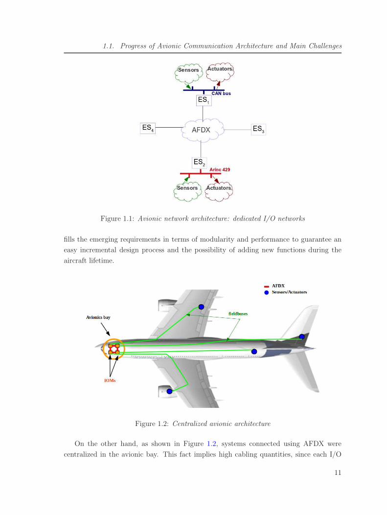
A380, consists of a high rate backbone network based on the AFDX [1] to interconnect
the critical subsystems, as shown in Figure 1.1. Then, each specific avionic subsystem is
directly connected to its associated Input/Output (I/O) network based on low rate data
buses, such as ARINC 429 [2] and CAN [3].
Although this architecture simplifies the design process and reduces the time to mar-
ket, it leads at the same time to inherent weight and integration costs due the important
number of sensors/actuators networks. In addition, this architecture makes the avionics
subsystems closely dependent on their Inputs/Outputs and no longer interchangeable.
However, for avionic applications, it is essential that the communication architecture ful-
10
1.1. Progress of Avionic Communication Architecture and Main Challenges
Figure 1.1: Avionic network architecture: dedicated I/O networks
fills the emerging requirements in terms of modularity and performance to guarantee an
easy incremental design process and the possibility of adding new functions during the
aircraft lifetime.
Figure 1.2: Centralized avionic architecture
On the other hand, as shown in Figure 1.2, systems connected using AFDX were
centralized in the avionic bay. This fact implies high cabling quantities, since each I/O
11

Chapter 1. Background and Problem Statement
network requires dedicated cabling to communicate with its corresponding AFDX end-
system. This cabling is done through long distances going generally from the aircraft
wings and tail, where most of sensors and actuators are located, to the main avionic bay
at the front of the aircraft.
Figure 1.3: Multi-cluster avionic network architecture
To handle these limitations, the solution, implemented in recent aircraft, such as A350
and A400M, consists in keeping the AFDX as a backbone network to interconnect the crit-
ical avionic systems, and dissociating the sensors and actuators from their corresponding
end-systems. As shown in Figure 1.3, the obtained clusters are interconnected via specific
devices, called Remote Data Concentrators(RDCs), and standardized as ARINC 653 [4].
RDCs are modular gateways distributed throughout the aircraft, as shown in Figure 1.4,
to handle heterogeneity between the AFDX backbone network and peripheral data buses.
This alternative architecture enhances the avionic subsystems modularity and simpli-
fies the reconfiguration process. The RDC actually becomes the main node that needs
to be reconfigured in case of sensor or actuator modification. Furthermore, distributing
RDC devices in the aircraft reduces considerably the required network cabling. However,
at the same time it represents one of the major challenges in the design process of such
multi-cluster avionic networks.
12

1.2. Description of Network Standards
Figure 1.4: Distributed avionic architecture
1.2 Description of Network Standards
In this section, we present the main features of the AFDX network used in current
avionic architectures as a high speed backbone network. Then, we describe the main
network technologies used for I/O networks: ARINC 429 and CAN.
1.2.1 ARINC 664: Backbone Network
The AFDX [1] network is based on Full Duplex Switched Ethernet at 100 Mbps, suc-
cessfully integrated into new generation civil aircraft, such as the A380 and the A400M.
This technology succeeds to support the important amount of exchanged data and to guar-
antee timing requirements, due to its high data rate, its policing mechanism in switches
and the Virtual Link (VL) concept.
1.2.1.1 Virtual Link
AFDX virtual link gives a way to reserve a guaranteed bandwidth to each traffic flow.
The VL represents a multicast virtual channel which originates at a single end-system
and delivers its packets to a fixed set of end-systems, as shown in Figure 1.5. Each VL is
characterized by: (i) BAG (Bandwidth Allocation Gap), ranging in powers of 2 from 1 to
128 milliseconds, which represents the minimal inter-arrival time between two consecutive
13

Chapter 1. Background and Problem Statement
Figure 1.5: Example of AFDX virtual links
frames; (ii) MFS (Maximal frame size), ranging from 64 to 1518 bytes, which represents
the size of the largest frame that can be sent during each BAG. The VL control mecha-
nism is illustrated in Figure 1.6.
Figure 1.6: Virtual Link bandwidth control mechanism
Using the VL control mechanism, a 100 Mbps Ethernet link can support multiple
Virtual Links. For instance, in Figure 1.7 three Virtual Links are carried by a single
Ethernet physical link. The figure also shows that the messages sent on AFDX Ports
1, 2, and 3 are carried as sub-VLs by VL 1. Similarly, messages sent on AFDX Ports 6
and 7 are carried by VL 2, and messages sent on AFDX Ports 4 and 5 are carried by VL 3.
1.2.1.2 Message flows & Frame Structure
The end-to-end communication of a message using AFDX requires the configuration
of the source end-system, the AFDX network and the destination end-systems to deliver
correctly the message to the corresponding receive ports. Figure 1.8 shows a message M
being sent to Port 1 by the avionics subsystem. End system 1 encapsulates the message
in an AFDX frame and sends it to the AFDX into the VL 100 (the destination addresses
are specified by VLID 100). The forwarding tables in the network switches are configured
14

1.2. Description of Network Standards
Figure 1.7: Three AFDX Virtual Links carried by a 100 Mbps Ethernet link
Figure 1.8: Example of application data flow on AFDX
to deliver the frame to both end-systems 2 and 3. The end-systems are configured to be
able to determine the destination ports for the message contained in the frame. In this
case, the message is delivered by end-systems 2 and 3 to ports 5 and 6, respectively.
15

Chapter 1. Background and Problem Statement
Figure 1.9: AFDX frame format
An AFDX frame is based on the Ethernet frame, as shown in Figure 1.9. The Ether-
net header allows the identification of the source and destinations end-systems. The IP
and UDP headers allow each destination end-system to find the corresponding destina-
tion port for the received message within the Ethernet payload. The Ethernet payload
consists of the IP packet (header and payload). Then, the IP packet payload contains
the UDP packet (header and payload), which contains the message sent by the avionics
applications. Padding is used only when UDP payload is smaller than 18 bytes, to ensure
a minimum AFDX frame size of 64 bytes. The maximum frame size is 1518 bytes without
counting the IFG (Inter-Frame Gap) of 12 bytes and the preamble of 8 bytes. This IFG
and preamble have to be considered when performing timing analysis to take into account
the overhead of data transmission over the AFDX network.
1.2.1.3 Application Layer: ARINC 653 Specifications
As shown in Figure 1.10, an avionics system is connected to the AFDX network through
an end-system. In general, an avionics system is capable of supporting multiple avion-
ics subsystems. A partitioning mechanism, compliant with ARINC 653 [5] specifications,
provides isolation between avionics subsystems within the same avionics system. This iso-
lation is achieved by restricting the address space of each partition and by placing limits
on the amount of CPU time reserved for each partition. The objective is to ensure that
an errant avionics subsystem running in one partition will not affect subsystems running
on other partitions.
Hence, avionics applications are assigned to ARINC 653 partitions and communication
between them is ensured using communication ports. In the example of Figure 1.11, three
AFDX end-systems communicate through an AFDX network. Each end-system runs two
16

1.2. Description of Network Standards
Figure 1.10: ARINC 653 partitioning for AFDX end systems
partitions which host avionics applications. Partition 1 of end-system 1 communicates
with partition 1 of end-system 2 using partitions ports (source port 1 of partition 1 of
end-system 1 and destination port 2 of partition 1 of end-system 2). As we can see from
this example, data flows originated from the same ARINC 653 partition in an AFDX
end-system can share the same VL at the MAC layer. However, data flows from different
partitions are not allowed to share VLs to guarantee segregation between partitions on
AFDX network.
1.2.2 Sensors/Actuators Networks
1.2.2.1 ARINC 429
The ARINC 429 standard [2] is a widely used avionic data bus that has been deployed
in various avionic applications for decades. This standard relies on unidirectional commu-
nications with a single transmitter and up to twenty receivers. Connected devices, Line
Replaceable Units (LRUs), can be organized in a star or bus topologies as shown in Figure
1.12. Each LRU may host multiple transmitters or receivers communicating on different
ARINC 429 buses. This simple architecture of ARINC 429 bus offers a highly reliable
17

Chapter 1. Background and Problem Statement
Figure 1.11: Communication from application to application over AFDX with ARINC 653
communication with short transmission latencies.
ARINC 429 data transfer is based on 32 bit data word, as described in Figure 1.13.
ARINC 429 data words are made up of five primary fields:
– Parity (1 bit): allowing error check to guarantee accurate data reception;
– Sign/Status Matrix (SSM) (2 bits): can be used to indicate the sign or direction
of the words data, or to report source equipment operating status. This field is
dependant on the data type;
– Data/Payload (19 bits): containing the word’s data information;
– Source/Destination Identifier (SDI) (2 bits): indicating which source is transmitting
the data or for which receivers the data is destined;
– Label (8 bits): is used to identify the word’s data type and can contain instructions
18

1.2. Description of Network Standards
Figure 1.12: ARINC 429 network architectures
or data reporting information. Labels may be further refined using the first 3 bits
of the data field as an Equipment Identifier to identify the source.
ARINC 429 specifies two speeds for data transmission: high speed operates at 100
Kbit/s and low speed operates at 12.5 Kbit/s. ARINC 429 operates in such a way that
each single transmitter communicates in a point-to-point connection with its receivers.
This fact requires an important amount of cables which significantly increases the overall
aircraft weight. This traditional data bus is no longer effective in meeting the emerging
requirements of avionic applications in terms of throughput demand and modularity.
Figure 1.13: ARINC 429 frame format
19

Chapter 1. Background and Problem Statement
1.2.2.2 CAN
The Controller Area Network (CAN) data bus was designed in the 80s by Robert Bosh
GmbH [3] for automotive applications. Its success due to its reliability and its versatility
attracted the attention of manufacturers in other industries, including process control,
medical equipment, and recently avionics.
The CAN bus operates at data rates up to 1Mbps for cable lengths less than 40m,
and 125Kbps when the length is around 500m. Two versions of the CAN protocol are
specified: CAN 2.0 A and CAN 2.0 B. The first uses the standard frame format, that
supports a 11-bit identifier, while the second uses an extended frame format in which the
identifier consists of 18 additional bits (for a total of 29 bits). Controllers connected to
the CAN bus must transmit and receive data while avoiding collisions using the Carrier
Sense Multiple Access with Collision Resolution (CSMA/CR) mechanism.
– Message arbitration: a bus terminal can start a new transmission only when the
bus is idle. However, if two terminals try to transmit at the same time, then an
arbitration protocol is implemented to allow the transmission of the message with
the highest priority (Arbitration based on Message Priority or AMP).
Figure 1.14: CAN protocol: CSMA/CR access mechanism
The bus signal can have two logic values, dominant and recessive: whenever two
terminals attempt a simultaneous transmission of a dominant bit and a recessive
bit, a dominant logic value will result on the bus. In a typical implementation of a
wired connection 0 is the dominant value, and consequently this is often called an
AND implementation. As shown in Figure 1.14, the first controller that loses the
contention, i.e., sending a recessive bit and reading a dominant value resulting on
20

1.2. Description of Network Standards
the bus, must immediately stop its transmission. This fact results in an arbitration
technique based on the message header, which determines the communication pri-
ority. CAN is based on broadcast communications where each transmitted frame is
received by all the connected terminals. Each node will determine if the received
frame is relevant to that particular system or not, and drop packets that were not
addressed to it.
– Frame structure as shown in Figure 1.15, CAN data frames consist of a payload
up to 8 bytes and an overhead of 6 bytes due to the different headers and bit stuffing
mechanism.
Figure 1.15: CAN 2.0 A frame structure
Each CAN frame consists of the following bit fields:
– Start Of Frame (SOF) (1 bit): is always a dominant bit marking the beginning
of a transmission;
– Arbitration (13 bits): consists of the Identifier, the Remote Transmission Request
(RTR) for a standard frame (or the Substitute Remote Request (SRR) for an
extended frame), and finally the Extension bit IDE to determine if the frame
is standard or extended. It identifies the type of CAN message and defines its
transmission priority on CAN bus;
– Control (5 bits): is composed of r0 and r1, reserved bits that are always dominant;
and the Data Length Code (DLC) of 4 bits, which specifies the number of bytes
present in the Data field;
– Data (1-64 bits): contains the actual information;
– CRC (16 bits): is used to guarantee data integrity;
– ACK (2 bits): allows receivers to acknowledge correct received messages;
21

Chapter 1. Background and Problem Statement
– End Of Frame (EOF) ( 7 bits): indicates the end of the CAN frame;
– Intermission Frame Space (IFS) (3 bits): is the minimum number of bits separat-
ing consecutive messages. During this intermission period no other communica-
tion can start on the CAN bus.
To ensure a strong synchronisation, the protocol avoids the presence of more than 5
consecutive bits of the same value in the transmitted frame by adding a stuffing bit
with the opposite value. Stuff bits increase the maximum transmission time of CAN
messages. Including stuff bits and the inter-frame space, the maximum transmission
time Cm of a CAN message m including bm data bytes were proven in [11] and are
given by the following expressions:
– for 11-bit identifiers,
Cm = (55 + 10 ∗ bm) ∗ τbit (1.1)
– and for 29-bit identifiers,
Cm = (80 + 10 ∗ bm) ∗ τbit (1.2)
where τbit is the transmission time for a single bit.
1.3 Description of RDC Standard: ARINC 655
The Remote Data Concentrator (RDC) [4] is a gateway that performs protocol conver-
sion to guarantee interoperability between avionic systems with different communication
interfaces and specific communication protocols. Typically, it translates data from various
sources, e.g. sensors and actuators, into a format usable by avionic computing resources.
It also converts data from computing resources into appropriate formats usable by various
sensors and actuators equipments. ARINC 655 standard [4] was introduced as a high-level
design guide for RDCs. It mainly reviews the requirements to fulfill by RDC devices for
avionic networks. Moreover, it provides guidelines concerning the design of RDC devices.
1.3.1 RDC Requirements
The RDC device inherits from avionics requirements described in Section 1.1.2.1 and
particularly:
22

1.3. Description of RDC Standard: ARINC 655
– Predictability: the process of reception and transmission of data by the RDC
device introduces additional network latency. For critical avionics applications, the
system designer must ensure that the end-to-end data latency is less than the re-
quired deadline. Therefore, it is important to determine the permissible latency for
each system that uses this information at the beginning of the design process.
– Reliability: the designer of RDC device should consider a fault tolerant design.
The level of fault tolerance is determined by the analysis of the system integrity
goals, the required availability of the function and the overall maintenance proce-
dure.
– Modularity: RDC device should be modular, i.e., composed of standard modules
that can be easily replaced. RDC devices should be exchangeable and reconfigurable,
such that the replacement of a RDC device does not require long and complex ad-
justments.
– Cost and life cycle: network designer should consider minimizing the different
types and number of required RDCs for an avionic network. This fact aims at
reducing manufacturing costs, by reducing the system weight and simplifying its
development.
Furthermore, an RDC device has to meet some additional requirements related to its
role as an interconnection device:
– Interoperability: the primary purpose of an RDC device is to ensure interoper-
ability of avionic systems of different manufacturers. Appropriate network interfaces
should be integrated into the RDC and data formats conversion functions should be
implemented to guarantee communication transparency between avionic systems.
The mapping of packets format has to be ensured between a source and a destina-
tion network interconnected by the RDC device.
– Adaptability: the RDC should be able to interface with a variety of data buses
and other network technologies used in aircraft. The RDC should be configurable to
be customized for different interconnection applications with different performance
requirements.
23

Chapter 1. Background and Problem Statement
– Resources utilization efficiency: the RDC should keep communication over-
heads as low as possible when forwarding data flows from a source to a destination
network. This fact saves network resources and keeps margins for the future evolu-
tion of the avionic architecture.
To meet the main RDC requirements, the ARINC 655 specifications provide some
recommendations and guidelines which can be grouped into two categories: functional
and architectural. These specifications will be detailed in the next sections.
1.3.2 Functional Specifications
The RDC device should include appropriate functions to receive, process and forward
data from typical avionic I/O networks to the processing computers and vice versa. The
main functions that should be integrated into the RDC device are:
– Data Mapping: the RDC should perform the conversion of the received data for-
mat to fit the target network format. A configurable mapping table should be used
to map data type and address to fit the requirements of the destination networks.
The mapping table should be static and well configured to guarantee the required
safety and timing performance levels. Furthermore, as several RDCs devices may
be used within the same network, a consistent mapping process should consider all
the mapping tables in RDC devices;
– Data Forwarding: the RDC should forward data received from an input network
interface to one or several output interfaces. The RDC may be used to connect two
or more network clusters. Therefore, a forwarding function is required to define for
each received data the output interfaces. A simple solution consists in using a static
forwarding table that is configured offline in the RDC device by the network designer;
– Data processing: the RDC may include software functions, such as data sampling,
filtering and monitoring. These software functions may also perform range checking,
data validity and fault detection. These functions may increase end-to-end commu-
nication latencies, and should be taken into account during the timing analysis and
the validation of the RDC behavior.
24

1.3. Description of RDC Standard: ARINC 655
1.3.3 Architectural Specifications
Figure 1.16: Synchronous mode for CAN-AFDX RDC
The main RDC’s architectural recommendations are:
– Communication scheme: two communication schemes are described in ARINC
653 specifications:
– Synchronous RDC: in this case, the processing and forwarding of a received data
by the RDC is triggered by the event of data reception. An example of a syn-
chronous CAN-AFDX RDC is shown in Figure 1.16.
– Asynchronous RDC: in this case, the rates and instants of data exchanges between
the RDC and connected networks are determined by the RDC. The RDC imple-
ments a write/read table where data from different equipments communicating
with the RDC are gathered. An example of an asynchronous CAN-AFDX RDC
device is shown in Figure 1.17. For each type of messages, a received message
in the RDC overwrites the old one and a binary freshness indicator is used. The
transmission of data flows is done periodically with transmission rates defined in
the RDC. One significant advantage of this asynchronous mode consists in adapt-
ing data rates between the source producing and the destinations receiving data.
For example, consider a sensor producing the air pressure measurement each 2
ms. Consider computing systems consuming this data to perform a computation
25

Chapter 1. Background and Problem Statement
once each 10 ms. Since sensor data is produced at a higher rate than the required
one, then the RDC may adapt production rates by reading the pressure data from
its write/read memory once each 10 ms.
Figure 1.17: Asynchronous mode for CAN-AFDX RDC
– Partitioning: the RDC should interconnect multiple sub-networks which may have
different levels of criticality. Therefore, a partitioning process should be used in the
RDC to keep isolation between communication flows having different criticality lev-
els.
1.4 Design Opportunities for Multi-Cluster Avionic
Networks
As described in Section 1.1.2.2, the main benefits of multi-cluster avionic networks are
the use of old equipments with new ones, and the reduction of weight and I/O resources.
For instance, the use of RDC devices allows cabling reduction, and enhances the modu-
larity and exchangeability of the avionic end-systems.
However, the use of multi-cluster networks in the avionics context arises mainly the
following challenges:
26

1.4. Design Opportunities for Multi-Cluster Avionic Networks
– Software/Hardware (SW/HW) Mapping: the avionics system consists of a
set of applications which need to exchange data; and a set of communicating nodes
via data buses or other network technologies. Each node can host one or multi-
ple applications. The mapping of applications onto network nodes is an important
task when designing the avionics networks. This mapping will clearly impact the
resource utilization and real-time performance of the avionics system, and it has to
be considered during network integration phase. Hence, the designer should select
the SW/HW mapping maximizing the resource savings while meeting real-time re-
quirements.
– End-to-end communication performance: avionics networks have to fulfill real-
time constraints requirements. Bounding the total delay of each data from a source
to one or many destination nodes is an important issue to fulfill the predictabil-
ity requirement, and particularly the stability for closed loop control in avionics. In
multi-cluster networks, the latency between data input and its corresponding output
are due to: (a) communication latency through network clusters (e.g. data buses
and backbone networks); (b) interconnection latency due to the traversal of gate-
ways. These delays depend on the scheduling policies used in the network nodes (e.g.
source and destination end-systems, switches and gateways), and the observed con-
tentions on shared networks. Hence, appropriate modeling and analysis techniques
should be used to prove that the avionics network meets the real-time requirements.
– Design of interconnection device and interoperability issues: the intercon-
nection devices have a major importance in multi-cluster avionics networks, since
they allow heterogeneous network technologies to exchange data and to keep end-to-
end connectivity between avionics systems. The RDC [4] is an avionics interconnec-
tion device used typically to connect sensors/actuators networks with the backbone
network connecting computing units. Therefore, the RDC device has: (i) to ensure
frame formats conversion and consistent addressing of data packets between source
and destination networks; (ii) to offer bounded latency and a predictable behaviour;
(iii) to ensure the isolation of data flows with different criticality levels. Further-
more, the inter-cluster communication through the RDC device may induce high
communication overheads due to the dissimilarities between interconnected network
clusters in terms of rates and frame formats. Hence, the impact of RDC device on
resource utilization has to be considered, and design choices reducing the commu-
nication overheads between interconnected networks should be integrated.
27

Chapter 1. Background and Problem Statement
1.5 Conclusion
Current civil avionic communication architecture consists of several network clusters,
interconnected using RDC devices standardized under the ARINC 655. These multi-
cluster networks present the advantage of allowing the use of old data buses in conjunction
with new network technologies, such as the AFDX protocol. This fact reduces develop-
ment costs of new equipments and guarantees the incremental design of avionics systems.
However, the performance optimization of multi-cluster avionic networks arise several
challenges, which are mainly due to: (i) the difficulty of performing software/hardware
mapping; (ii) the complexity of performance analysis and meeting the real-time con-
straints; (iii) the design of interconnection devices and interoperability issues.
In the next chapter, we present the main related work on performance optimization
for multi-cluster embedded networks, and especially the main existing work dealing with
the interconnection devices.
28

Chapter 2
Related Work: Performance
Optimization for Multi-Cluster
Networks
In the area of performance optimization for embedded networks in avionics and au-
tomotive, various approaches have been integrated into different parts of the end-to-end
communication path, including traffic sources, communication networks and interconnec-
tion devices. We review in this chapter the most relevant work in this area for avionics
and automotive applications. First, we present optimization approaches for traffic-source
mapping, where the main concern is the mapping of the application data onto frames.
Then, main existing approaches for performance optimization for communication net-
works are detailed, including, timing analysis and data routing for both AFDX and sen-
sors/actuators networks. Finally, the optimization of interconnection devices is reviewed
and existing protocol conversion approaches to guarantee real-time performance and re-
source utilization efficiency are detailed.
2.1 Optimizing Traffic-Source Mapping
Traffic-source mapping consists in affecting data produced by a source application to
the frames supported by the communication network. A simple mapping consists in in-
cluding each generated data into a dedicated frame. However, this choice may induce a
high communication overhead. A more advanced mapping approach consists in grouping
multiple data produced by one or many applications in the same network frame. The
traffic-source mapping has a direct impact on the network utilization. The grouping pro-
29

Chapter 2. Related Work: Performance Optimization for Multi-Cluster Networks
cess of elementary data allows reducing the protocol overheads, and consequently saving
network capacity and improving communication efficiency. Different strategies have been
introduced for avionics end-systems and automotive ECUs (Electronic Control Units) and
have shown significant enhancements in terms of network capacity utilization.
2.1.1 Avionics End-Systems
The AFDX network is considered as a promising communication technology for mod-
ern avionics architectures. The AFDX is based on routing frames through isolated data
channels, called Virtual Links (VLs).
In [12], the authors introduced a method to define VLs characteristics to minimize
the AFDX network utilization rate. The method presented in [12] is illustrated in Figure
2.1 and it consists in packing data from different AFDX applications hosted by the same
AFDX end-system within the same AFDX frame. The transmission of each resulting
AFDX frame is supported by an AFDX VL respecting the frame characteristics. The
authors in [12] proposed an approach to find VLs configuration minimizing the band-
width consumption on AFDX network to improve network resources utilization and to
ease the addition of new VLs. First, an algorithm to find the optimal VLs allocation for
periodic or sporadic data generated by the same AFDX application was proposed. This
algorithm is based on data segmentation and has as objective minimizing the consumed
bandwidth on the AFDX network. Afterwards, this algorithm was extended to find the
optimal allocation for a set of data generated by the same end-system. The applicability
of this approach was illustrated on a representative avionics benchmark, and the results
showed its efficiency to save network bandwidth utilization. However, this approach did
not integrate the verification of the time constraints.
Another interesting work in this area was presented in [13]. This work concerns the
adequate mapping of avionics functions onto processing modules while meeting real-time
and resource constraints. Avionics applications are hosted by partitions compliant with
ARINC 653 [5]. Each partition has its own memory space and it is executed periodically
during a reserved time slot. As illustrated in Figure 2.2, two partitions P1 and P2 are
executed on the same processing unit with respect to their associated periods. The period
of the obtained schedule is called the Major Frame (MAF).
In [13], the authors formulated an optimization problem for mapping avionics par-
titions onto processing resources of an IMA architecture. The formulation takes into
30

2.1. Optimizing Traffic-Source Mapping
Figure 2.1: Data packing and VLs allocation
Figure 2.2: Periodic execution of Partitions
account resources as well as timing constraints of mapped avionics functions. The main
objective was to maximize the evolution margins and to ease future avionics functions
addition to the system. A method to solve this optimization problem was provided.
However, this mapping problem considered only AFDX communication network, and the
impact of an interconnected communication network, as currently used in avionics, on the
software/hardware mapping was not considered.
31

Chapter 2. Related Work: Performance Optimization for Multi-Cluster Networks
2.1.2 Automotive End-Systems
For automotive applications, mapping periodic or sporadic data flows produced by
applications sharing the same ECU onto frames has been widely studied to minimize
bus utilization rate. Frame packing is a classic technique used in automotive context to
achieve this aim. In [14] and [15], authors proposed the use of frame packing to allocate
signals produced by source applications to CAN frames. This approach is illustrated in
Figure 2.3. The proposed frame packing strategy consists in fixing the groups of data to
pack based on an arbitrary criterion. Then, a periodic CAN frame is defined per group of
data respecting the maximal CAN payload size. In [14] and [15], the authors proved that
the data packing problem is NP-hard and proposed several algorithms to select adequate
frame packing strategies processed in a polynomial time. A comparative study of the dif-
ferent algorithms has been conducted to select the most resource efficient configuration.
However, these methods assume a synchronous behaviour of the different applications
hosted by the same ECU. This assumption is not always verified in the general case and
the proposed method could be complex to generalize.
Figure 2.3: Data packing of CAN frames
In [16], the authors considered a multi-cluster communication architecture, as de-
scribed in Figure 2.4. This architecture consists of two heterogeneous communication
buses: Event-Triggered and Time-Triggered. For instance, authors considered CAN bus
as a representative technology of event-triggered data buses, and TTP/C as a representa-
tive technology of time-triggered data buses. A gateway is used to support communication
between both data buses. In [16], the authors proposed a frame packing strategy inside
source nodes of both network clusters, to achieve higher bus utilization rate and to im-
prove flows schedulability. In this approach, the timing constraints of messages were
integrated, and a schedulability analysis which takes into account the queuing delays in
the gateways was provided. However, The frame packing was implemented only in source
nodes, while the gateway was considered as a simple conversion node, e.g., each received
32

2.2. Optimizing Communication Network Performance
frame in the gateway from a source cluster implies exactly one forwarded frame to the
other cluster. Although this approach showed interesting bandwidth consumption sav-
ings, further enhancements may be achieved by considering the role of the gateway in
reducing communication overheads.
Figure 2.4: Multi-cluster automotive network architecture
2.2 Optimizing Communication Network Performance
Various analytical methods have been introduced to compute end-to-end communica-
tion latencies. These methods were used in the literature to analyze and optimize the
performances of critical embedded networks. Furthermore, routing algorithms have been
studied for embedded networks to improve network timing performances and to guarantee
a better load balance in the network. First, we present the main related work to AFDX
performance analysis and optimization. Then, we give an overview of the main work
concerning sensors/actuators networks.
33

Chapter 2. Related Work: Performance Optimization for Multi-Cluster Networks
2.2.1 Work on the AFDX Network
2.2.1.1 Timing Analysis techniques
In avionics networks, for certification reasons, it is necessary to prove that the com-
munication latency for each message does not exceed its deadline. To achieve this aim,
several techniques have been introduced in the literature to analyze the timing perfor-
mance of avionics networks. In particular, the AFDX network has been largely studied
and several methods to prove the predictability of communication over AFDX has been
proposed such as Network Calculus [17], Trajectory approach [18] and Model checking
[19]. These methods can be organized into two categories:
– Methods computing an upper bound on end-to-end communication delays: Network
Calculus and Trajectory approach
– Methods computing the exact end-to-end communication delays: Model checking
TheNetwork Calculus (NC) formalism is based on the mathematical theory of Min-
Plus algebra [20]. This theory has been widely used for analyzing performance guarantees
in computer networks, and it was one of the first methods used for AFDX certification
[17] [21].
To provide timing guarantees for data flows, Network Calculus formalism is based on
bounding network resources. This means that traffic sources have to guarantee a maxi-
mum traffic emission, and network elements have to offer guarantees on minimum service
capacity. To model the data flows generated by sources in the network, the concept of
arrival curve is used. Then, to model the amount of service guaranteed by a network node
applying some scheduling policy, the concept of service curve is used. Given the model
of an input data flow and the model of the traversed network node, Network Calculus
provides a bound on the maximal traversal delay of the network node using the horizontal
deviation between the arrival curve and the service curve. Furthermore, a characterization
of the output traffic from the network node using arrival curves is provided. More details
about Network Calculus theory can be found in Appendix A.
In [17], the authors introduced a methodology for modeling the AFDX network using
Network Calculus formalism. The AFDX data flows were modeled using arrival curves,
deducted directly from the VLs characteristics, i.e., maximum frame size and minimum
inter-arrival time. Moreover, each network node was modeled using service curve which
34

2.2. Optimizing Communication Network Performance
takes into account the respective scheduling policy. Then, a method for computing the
end-to-end delay bound for a given AFDX flow has been introduced. This timing analysis
method consists in propagating the arrival curve of a given data flow from the source
end-system to the destination end-system throughout its path.
This timing analysis method based on propagating arrival curves offers upper bounds
for end-to-end delays in AFDX networks. However, this approach [17] leads to pessimistic
bounds, as the serialization of frames is not taken into account between two successive
nodes. Consider two AFDX flows traversing a tandem of network nodes, the application
of the propagation analysis approach integrates twice the impact of a flow on the other (at
the first node and at the second node). To achieve tighter bounds on AFDX end-to-end
delays, the authors used a ”grouping” technique [21]. This technique takes into account
the serialization of frames from different VLs transmitted on the same AFDX link. The
”group” is defined as the set of VLs which exit from the same switch output port and enter
the same switch input port, i.e. Virtual Links that share at least two segments of path.
The key issue is that the frames of those VLs are serialized once when exiting the first
output port. This optimized technique has been shown to offer tighter bounds compared
to the propagation algorithm. However, since the first applications of Network Calculus
to AFDX network, a multitude of Network Calculus algorithms have been proposed in
the literature. Achieving tighter bounds with Network Calculus requires an increasing
computational complexity. Therefore, there is a trade-off between the quality of the ob-
tained upper bounds on network traversal delays and the computational complexity of
the Network Calculus algorithms.
The Trajectory approach is a timing analysis technique introduced to get upper
bounds on communication response times in distributed systems [22] [23]. For each packet
from a given flow, the trajectory approach builds the packets sequence corresponding to
the worst-case in each traversed node. The end-to-end delay is then deducted from delays
experienced in crossed nodes throughout the packet path.
To explain the trajectory approach, we consider the example of the communication
network in Figure 2.5. The communication network is composed of seven connected nodes.
Each data flow follows a path in the network corresponding to the crossed nodes from
end-to-end. This path is assumed to be static in the Trajectory approach and the set of
crossed nodes by the data flow can be seen as an ordered sequence of nodes. In the exam-
ple of Figure 2.5, two flows are considered, τ1 and τ2. τ1 follows the path P1 = {4, 5, 6, 7}.The Trajectory approach assumes, with reference to a flow τi with path Pi, a flow τj with
path Pj , such that Pi 6= Pj and Pi ∩ Pj 6= ∅. In the example of Figure 2.5, flows τ1 and
35

Chapter 2. Related Work: Performance Optimization for Multi-Cluster Networks
Figure 2.5: Example of communication network
τ2 verify the assumption of trajectory approach since P2 = {1, 5, 6, 3} and P1∩P2 = {5, 6}.
Flows are scheduled in each crossed node. Each flow τi has a minimum inter-arrival
time between two consecutive packets at the first node of its path in the network. The
end-to-end delay of a packet computed using the Trajectory approach is the sum of the
times spent in each visited network node and the transmission delays on links. Consid-
ering a FIFO (First In First Out) scheduling algorithm, the time spent by a packet m
in node h depends on the pending packets in h at the arrival time of m to h. In the
worst-case, all these pending packets are more prior than m and will be processed before
m.
In [18], the trajectory approach has been applied to AFDX network by considering
that:
– An end-system is represented by a node in the trajectory approach;
– Each output port of an AFDX switch is represented by a node in the trajectory
approach;
– The switches latency is represented by links in the trajectory approach;
– An AFDX VL becomes a flow in the trajectory approach.
The authors conducted a comparison between results obtained using the propagation
algorithm with Network Calculus and those obtained using Trajectory approach. Ob-
tained results showed that the upper bounds on the end-to-end delays on AFDX obtained
using the Trajectory approach are tighter compared to Network Calculus bounds.
36

2.2. Optimizing Communication Network Performance
The Model checking [19] is another approach to guarantee the maximum trans-
mission delay in the AFDX network, which computes the exact worst-case end-to-end
communication delays. The basic idea of this approach consists in checking all the possi-
ble scenarios that the network can experience to find the exact worst-case communication
delays. These scenarios form an exploration space which is often called ”state-space”. An
attempt for applying the Model Checking approach to analyze the performance of AFDX
network was done in [24]. A major difficulty is that, theoretically, the state-space of
AFDX communication network is infinite (because of continuous real-time nature of the
network). Therefore, using model checking for such applications requires some kind of
state-space reduction. Unfortunately, the use of Model Checking is yet limited compared
to Network Calculus and Trajectory approach, as it cannot cope with realistic AFDX
networks, due to the combinatorial explosion problem for large configurations.
In our case, we conduct timing analysis of the AFDX network using Network Calculus
approach due to its low computational complexity. Furthermore, we developed a perfor-
mance analysis tool for avionics networks based on Network Calculus formalism, called
WoPANets [6] (see Appendix A for more details).
2.2.1.2 Optimal Routing for AFDX
The AFDX network is a switched network with multiple possible paths from a given
source to a destination end-system. As we explained in Section 1.2.1, in AFDX networks,
VLs are routed statically. One major task when integrating the avionics architecture con-
sists in defining VLs paths throughout the AFDX network. In [12], the authors addressed
the optimization of VLs routing for the AFDX network to minimize communication la-
tencies and to limit the maximum utilization rate of the AFDX links. Indeed, a poor VL
routing may induce a high contention level between AFDX flows at the output ports of
the AFDX switches, and consequently inducing high communication latencies. To over-
come this problem, the authors in [12] proposed a routing algorithm that can be used to
route thousands of VLs, to maximize the minimal residual capacity of the AFDX links.
The main idea of this algorithm is to balance the communication load between network
switches and to keep a low contention level. This fact leads to low traversal delays of the
switches, and consequently low end-to-end latencies on the AFDX network. This tech-
nique optimizes the network resources utilization and lets margins for network evolution.
37

Chapter 2. Related Work: Performance Optimization for Multi-Cluster Networks
Figure 2.6: Optimization of sensors/actuators network performance
2.2.2 Work on Sensors/Actuators Networks
Different I/O buses may be used in multi-cluster avionics networks as shown in Figure
2.6. The timing analysis of these data buses is necessary to prove the predictability of the
avionics system. This problem has been addressed for CAN bus [25] to prove its timing
guarantees and thus the predictability of communications. The objective is to prove that
the response time of a message, which needs to be delivered from a source to one or many
destination nodes on the bus, does not exceed its Deadline.
The CAN bus has been largely used as the main communication network for auto-
motive applications. Many approaches have been proposed in the literature for timing
analysis of CAN bus to prove its capacity to meet strict real-time constraints of automo-
tive applications. In [25], Tindell et al. were the first to introduce a method to compute
exact Worst Case response Time (WCRT) on CAN bus. This result was proven to be
optimistic under certain conditions by Davis et al. in [11] and a revision of the method
introduced in [25] was provided. In [11], the Worst Case Response Time (WCRT) on
CAN for a message m is given by:
Rm = maxq=0..Qm−1
Rm(q) (2.1)
(2.2)
38

2.2. Optimizing Communication Network Performance
where Qm is the number of instances of message m that become ready to transmission
before the end of the busy period relative to m, and Rm(q) is the WCRT of instance q of
message m. Rm(q) is given by:
Rm(q) = Cm + Jm + wm(q)− qTm (2.3)
(2.4)
where,
– The transmission time Cm, corresponding to the longest time that the message can
take to be transmitted;
– The queuing jitter Jm, corresponding to the longest time between the initiating
event and the message being queued, ready to be transmitted on the bus;
– The queuing delay wm(q), corresponding to the longest time that the instance q of
messagem can remain in the CAN controller queue, before commencing transmission
on the bus;
– Tm is the period of message m.
wm(q) is computed using the following iterative expression:
wn+1m (q) = Bm + qCm +
∑
k∈hp(m)
⌈wn
m + Jk + τbitTk
⌉∗ Ck (2.5)
where hp(m) corresponds to the set of messages with priority higher than m, τbit
the transmission time of one bit and Bm the maximum blocking time due to the set of
messages with lower priority than m, denoted by lp(m):
Bm = maxk∈lp(m)
Ck (2.6)
The number of instances that need to be examined Qm is given by:
Qm =
⌈tm + Jm
Tm
⌉(2.7)
where tm corresponds to the length of the priority level-m busy period, which is given
by the following recurrence relation, starting with an initial value of tm = Cm, and finishing
39

Chapter 2. Related Work: Performance Optimization for Multi-Cluster Networks
when tn+1m = tnm:
tn+1m = Bm +
∑
k∈hep(m)
⌈tnm + Jk
Tk
⌉∗ Ck (2.8)
hep(m) is the set of messages with priority higher or equal to m.
These expressions were introduced for native CAN protocol, which assumes a Static
Priority (SP) queues in all CAN nodes to schedule messages sharing the same CAN source
node. However, different CAN bus configurations have been investigated and the timing
analysis in [11] has been adapted to fit the following CAN configurations:
– CAN bus with SP and FIFO queues: in [26], the WCRT analysis for CAN bus
has been extended to cover the case where CAN nodes may implement SP or FIFO
queues. This work was motivated by the fact that some CAN devices implement
queueing policies that are not strictly SP-based, thus invalidating the assumption
of SP queues for CAN nodes with the native CAN bus. The authors in [26] showed
that using FIFO queues instead of SP queues in CAN nodes significantly degrade
the overall real-time performance of the network. Therefore, they recommended the
use of priority queues whenever possible. However, system integrators do not always
have control over the queuing policies implemented in the communications stacks or
devices of all the ECUs of the system. In this case, the analysis in [26] may be useful.
– CAN bus with offsets: in [27], the WCRT analysis for CAN bus has been ex-
tended to cover the case where the production of messages in CAN nodes is desyn-
chronised using offsets. Transmitting frames with offsets means that the first in-
stance of a stream of periodic frames is released with a delay, called the offset, with
regard to a reference point. This latter is the first instant at which the station
becomes ready to transmit. The frames are then sent periodically, with the first
transmission as the time origin. It is worth noticing that since there is no global
synchronization among the CAN stations, each station possesses its own local clock
and the de-synchronization between the streams of frames remain local to each sta-
tion. Unlike the native CAN analysis which is based on a synchronous transmission
of frames by a CAN source, using offsets allows to avoid this worst-case scenario,
and thus reduce WCRT on CAN bus. The authors in [27] proved that using offsets
in CAN sources is beneficial in terms of reducing response times, especially at high
CAN loads.
40

2.3. Optimizing Interconnection Devices
2.3 Optimizing Interconnection Devices
The use of interconnection devices for multi-cluster networks has become very common
in automotive and recently in avionics context. These devices allow different communi-
cation standards and equipments to coexist with each other. As automotive and avionics
networks are subject to strict real-time constraints, proofs of determinism and reliability
have to be provided. As a main part of such networks, interconnection devices should be
designed to guarantee correct protocol conversion between network clusters and real-time
requirements, and to enhance network efficiency. In automotive and avionics context,
several approaches concerning the interconnection device design and performance opti-
mization have been proposed.
2.3.1 CAN-Ethernet Bridge
In [28], authors proposed a mixed CAN-Ethernet network architecture as an alterna-
tive to interconnected CAN buses. As the CAN [3] bus has limited number of supported
nodes, i.e., 30 nodes at 1 Mbps, and a relatively low transmission rate compared to Eth-
ernet, the authors proposed an extended CAN architecture where multiple CAN buses
communicate with each other through Ethernet bridges, as shown in Figure 2.7.
Figure 2.7: CAN-Ethernet communication architecture
41

Chapter 2. Related Work: Performance Optimization for Multi-Cluster Networks
This mixed CAN/Ethernet network allows connecting a high number of CAN terminals
and consequently balancing CAN utilization and improving its scalability. Furthermore,
a frame packing technique was implemented in the CAN-Ethernet bridges to reduce the
induced overhead by CAN traffic on the Ethernet. This frame packing technique consists
in encapsulating several CAN frames into the same Ethernet frame while respecting the
maximum frame size of 1518 bytes. Furthermore, the bridge decapsulates the CAN frames
received within an Ethernet frame and transmits these CAN frames to their final desti-
nations. To analyze the network performances, the average communication latencies were
analyzed using simulation. This approach is not sufficient to prove the communication
determinism and the worst-case behavior required by critical embedded networks.
2.3.2 CAN-FlexRay Gateway
In modern cars, CAN [3] is the dominant network protocol for in-vehicle communi-
cation. However, as discussed in [29], CAN reached its limits in terms of data rate (a
maximum rate of 1 Mbit/s) and maximal number of supported ECUs with the emergence
of x-by-wire applications, i.e., the replacement of mechanical and hydraulic systems by
electronic ones. This fact increases the number of in-vehicle functions and exchanged
data volume. CAN is based on an Event-Triggered arbitration mechanism, which may
induce high jitter under high utilization rates. The emerging FlexRay protocol, which
has a higher transmission capacity of 10 Mbit/s and supports both time-triggered and
event-triggered traffic, is expected to meet the emerging requirements of automotive ap-
plications. However, as the technology transition from CAN to FlexRay could not happen
at once, both network protocols are expected to be used together in automotive in the
near future. Consequently, the applications requiring low speed will still be carried out
by CAN bus, while new high-speed functionality will be implemented on FlexRay network.
This situation imposes the existence of a gateway unit, which facilitates the inter-
communication between CAN and FlexRay networks. In [29], a gateway for CAN and
FlexRay interconnection for in-vehicle networks was proposed. The considered commu-
nication architecture is described in Figure 2.8. Authors addressed the design of high-
performance gateway, offering efficient resource utilization.
42

2.3. Optimizing Interconnection Devices
Figure 2.8: CAN-FlexRay communication architecture
Figure 2.9: CAN-FlexRay Gateway functional structure
The proposed gateway in [29] to interconnect CAN and FlexRay networks, is shown
in Figure 2.9. Each frame received in the gateway from a source bus is first decoded. The
frame is then processed to get the data included in the frame. The protocol conversion
is then undertaken, i.e., the conversion of data from one protocol format to another. The
data is inserted into an appropriate frame and then coded for transmission on the des-
tination bus. For example, the protocol conversion operation from FlexRay to CAN is
shown in Figure 2.10. To transmit a FlexRay message on CAN bus, the CAN-FlexRay
43

Chapter 2. Related Work: Performance Optimization for Multi-Cluster Networks
gateway will check if the message is compatible for transmission on the network, i.e., less
than or equal to 8 bytes. If the message meets the criteria, then it will be inserted into the
transmission buffer. If the message is too large, then the gateway will send the message
to the transmit buffer sequentially in blocks of 8 bytes until no remaining data has to be
transmitted.
Figure 2.10: CAN-FlexRay Gateway operation diagram
The performance analysis of the CAN-FlexRay gateway, based on an experimentation
platform, has shown bounded processing delays with low jitter. In our work, we address a
similar problem for avionics networks which consists in interconnecting CAN and AFDX
44

2.3. Optimizing Interconnection Devices
networks. Our objective is designing an efficient gateway in terms of resources utilization,
while meeting the timing constraints. However, the protocol characteristics of FlexRay
are different from those of AFDX networks, especially in terms of communication schemes
and frame formats. This fact makes the interconnection approach of [29] inapplicable in
our case. Furthermore, this approach was limited to the functional aspects of the gateway
design, whereas architectural aspects were not addressed. In our case, both functional
and architectural perspectives are detailed to cover the different aspects which impact the
CAN-AFDX RDC performance and resource utilization efficiency.
2.3.3 ARINC 429-AFDX Gateway
The transition of ARINC 429 systems to AFDX-compliant systems cannot be done in
a short time. Hence, both networks need to coexist for a while and aircraft manufacturers
opted for a gatewayed architecture. As described in Appendix B of ARINC 664 [1], a
gateway device may be used to convert ARINC 429 messages to AFDX frames and vice
versa. The gateway proceeds as follows: it encapsulates multiple ARINC 429 messages
into the same AFDX frame to be then transmitted on the AFDX; and it decapsulates sev-
eral ARINC 429 messages received within the same AFDX frame to be then transmitted
on the ARINC 429.
Figure 2.11: Example of AFDX frame including multiple ARINC 429 labels
An AFDX frame formatting mechanism, which allows a network designer to better
45

Chapter 2. Related Work: Performance Optimization for Multi-Cluster Networks
map non-AFDX data onto AFDX messages is provided in [1]. An illustrative example of
the formatting of packed AFDX frames is given in Figure 2.11. In this example, 4 ARINC
429 frames are included into the same AFDX frame. However, no details are given on
how to select groups of data to include within the same AFDX frame. Furthermore,
performance analysis and optimization are left to the attention of network designers.
2.4 Need for Optimized CAN-AFDX Gateway
CAN bus has been successfully used for decades in automotive due to its high relia-
bility, real-time properties and low cost. It became recently an attractive communication
technology for aircraft manufacturers. Recent standards for avionics have been intro-
duced, such as CANAerospace [30] and ARINC 825 [31]. A typical avionics network
architecture is shown in Figure 2.12 where CAN buses are used as sensors/actuators net-
works. The communication with processing units connected to the high speed backbone
AFDX network is ensured using RDC devices [4]. The main role of these devices is to
handle protocol dissimilarities between AFDX and CAN and to guarantee interoperability
between them.
Figure 2.12: CAN-AFDX avionics architecture
Although the RDC was introduced to interconnect communication networks in avion-
ics context, few works have addressed the design of RDC devices to interconnect CAN and
46

2.4. Need for Optimized CAN-AFDX Gateway
AFDX networks. The objective of our current work is to design an enhanced CAN-AFDX
RDC, which offers a high network efficiency and guarantees system’s requirements. The
CAN-AFDX RDC should:
– correctly convert CAN frames to AFDX frames, and vice versa;
– ensure a consistent addressing between CAN and AFDX networks;
– guarantee temporal constraints of data flows from end-to-end;
– be optimized to achieve a high network efficiency in terms of resource savings.
To achieve this goal, our proposal is based on extending the RDC device standard
[4] by adding new functions, to improve system’s performance and enhance network effi-
ciency. The main heterogeneity parameters between CAN and AFDX networks concern
the communication paradigms, data rate and frame characteristics dissimilarities. The
CAN is a multiplexed bus with a CSMA/CR access mechanism based on static priorities,
whereas the AFDX is a switched network based on virtual link concept. CAN frames can
support a maximal payload of 8 bytes which is very small compared to an AFDX frame,
which can support up to 1472 bytes of payload. The main arising issues to design and
validate a CAN-AFDX RDC device are as follows:
– RDC design: the key function of this specific equipment is to keep the communi-
cation transparency between an AFDX calculator and a CAN sensor or actuator to
avoid the alteration of existent hardware in these equipments. Hence, for an AFDX
calculator the source or the destination of the transmitted Virtual Link is the RDC
device, while for a CAN sensor or actuator the transmitted data is consumed or
generated by the interconnection equipment. The main characteristics of the CAN-
AFDX RDC to define are:
– gateway strategy and addressing scheme: we need to define an accurate method
to map CAN frames onto AFDX VLs. A first basic strategy consists in associat-
ing for each CAN frame one AFDX VL using a static mapping table. This latter
method will be shown to be non optimal in terms of reserved bandwidth on AFDX;
– data formatting: the gateway strategy implementation requires an appropriate
data formatting to send one or many CAN frames on the same AFDX VL. The
47

Chapter 2. Related Work: Performance Optimization for Multi-Cluster Networks
choice of this structure should take into account the AFDX standard, and reduce
as much as possible the induced overhead to guarantee the bandwidth consump-
tion efficiency on the AFDX;
– data routing: the RDC device should be capable to interconnect several I/O CAN
buses to the AFDX backbone. The RDC should implement a routing mechanism
which forwards each input data to its corresponding output RDC interface(s);
– flows segregation: when connecting multiple I/O CAN buses with different crit-
icality levels to the AFDX using the same RDC device, an adapted segregation
mechanism should be implemented in the RDC to guarantee the isolation between
the different criticality levels.
– Performance analysis and optimization of RDC: the RDC device should be
designed to fulfill avionics requirements in terms of predictability and resource effi-
ciency. Hence, the main challenges are:
– Timing analysis: for avionic embedded applications, it is essential that the com-
munication network fulfills certification requirements, e.g. predictable behavior
under hard real-time constraints and temporal deadlines guarantees. The use
of gateways may increase the communication latencies and real-time constraints
have to be met. To deal with the worst-case performance analysis of such network,
an appropriate timing analysis has to be considered;
– Optimization process: to increase the network efficiency, especially in terms of
bandwidth consumption on the AFDX, and to enhance margins for future avionic
functions addition, an optimization process of the RDC parameters is required.
This process will define the most accurate RDC configuration, which respects
the system’s constraints and minimizes the induced network overhead, and con-
sequently consumed network resources.
2.5 Conclusion
In this chapter, we reviewed the main related work in the area of performance op-
timization for multi-cluster embedded networks, especially those addressing the design
of interconnection devices in avionics and automotive. In automotive context, several
48

2.5. Conclusion
techniques to enhance the gateway design, and consequently network performance have
been proposed. However, there are less approaches addressing efficient gateways design
in avionics context. Hence, there is a clear need for an optimized avionics gateway, and
particularly one to interconnect CAN and AFDX networks. The main arsing issues to
design this latter were detailed to enhance the system’s performance and resource savings.
In the next chapter, we will detail the design of our proposed RDC device to handle
the identified issues.
49

Chapter 2. Related Work: Performance Optimization for Multi-Cluster Networks
50

Chapter 3
Design of an Enhanced CAN-AFDX
RDC
In this chapter, we introduce an enhanced RDC device for CAN-AFDX networks to
improve the system’s performances. Compared to the current RDC device, new functions
are integrated to maximize the network resource savings and to guarantee real-time perfor-
mances. First, the current RDC device is described and will be considered as a reference
to highlight the introduced enhancements within the proposed RDC device. Then, the
functional structure overview of our proposed RDC device is presented. Finally, we detail
the implemented functions within this latter, such as frame packing and traffic shaping
mechanism.
3.1 Current RDC Device
In Figure 3.1, the currently used CAN-AFDX RDC device is presented to show the
main characteristics of the current implementation. This RDC performs the frame con-
version from CAN to AFDX, and vice versa using a mapping table. Data mapping is a
necessary function of the RDC device connecting two network protocols with dissimilar
addressing schemes. The mapping is defined within a static table which is configured
offline and does not change during execution time. Within the current RDC device, the
data mapping function is based on a static table associating for each CAN ID an AFDX
VL ID, since no packing process is performed. This mapping is illustrated in Table 3.2,
where three CAN messages required three dedicated VLs.
The main characteristics of the current RDC are:
51

Chapter 3. Design of an Enhanced CAN-AFDX RDC
Figure 3.1: Current CAN-AFDX RDC functional structure
Figure 3.2: Mapping table for the current RDC device
– (1:1) conversion strategy: as shown in Figure 3.3, it proceeds as follows: first,
each frame received at the input interface is decapsulated to extract the payload.
Then, based on the static mapping table, the required header is identified and added
to the extracted payload to build the corresponding frame at the output. This latter
is then sent through the target network interface.
52

3.1. Current RDC Device
Figure 3.3: The current CAN-AFDX RDC: (1:1) strategy
– One-to-one interconnection: as illustrated in Figure 3.4, the current RDC can
connect only one I/O bus to the AFDX. Thus, one RDC device is required per I/O
network interconnected to the AFDX.
Figure 3.4: Current CAN-AFDX RDC interconnection topology
As it can be noticed, the (1:1) strategy of the current RDC device is simple to imple-
ment. However, it can induce high bandwidth consumption on the AFDX network. For
the CAN-AFDX case study, implementing the (1:1) strategy in the RDC device consists
in forwarding one AFDX frame with a minimum size of 84 bytes AFDX frame (IFG (Inter
Frame Gap) included) for each received CAN message with a maximum payload size of
8 bytes. This clearly induces a high overhead on the AFDX network, and consequently
53

Chapter 3. Design of an Enhanced CAN-AFDX RDC
a poor network utilization efficiency. Furthermore, the use of one RDC device per inter-
connected I/O network can lead to high hardware costs and important system’s weight.
3.2 Enhanced RDC Functional Overview
To overcome the limitations of the current RDC, we propose an enhanced CAN-AFDX
RDC with: (i) additional functions to reduce communication overheads and to maximize
resource savings; (ii) the possibility to connect multiple I/O networks using one RDC
device based on a software partitioning mechanism.
A modular structure of our proposed RDC is shown in Figure 3.5. It has one AFDX
interface to communicate with AFDX end-systems and several CAN bus interfaces to
communicate with several I/O CAN buses. Each network interface in the RDC consists
of a reception interface denoted by Rx and a transmission interface denoted by Tx. For
each CAN bus, a compliant-ARINC 653 [5] partition is implemented to ensure commu-
nication isolation between the different CAN buses. This choice is mainly motivated by
the safety requirements, especially the need to limit errors propagation. Furthermore, we
consider the synchronous communication scheme described in Section 1.3.3.
Figure 3.5: Enhanced CAN-AFDX RDC functional structure
Each partition handles upstream and downstream flows originating or destined to
its associated CAN bus to or from the AFDX. Furthermore, an I/O processing unit is
54

3.2. Enhanced RDC Functional Overview
required to forward a data received on the input AFDX interface to the appropriate par-
tition, based on a pre-configured forwarding table.
The main new functions added to the basic RDC are:
– Frame packing function: is applied to upstream flows to reduce communica-
tion overhead. Frame packing of upstream flows consists in grouping several CAN
data into a single AFDX frame, as shown in Figure 3.6. This fact allows to reduce
required AFDX overhead, and thus AFDX bandwidth consumption to forward up-
stream flows from a CAN bus to the AFDX network;
Figure 3.6: Packing CAN messages into AFDX frames
– Frame unpacking function: is applied to downstream flows. It consists in ex-
tracting multiple CAN data from a single AFDX frame when the frame packing
process is activated at the AFDX source. In [12], authors introduced a frame pack-
ing algorithm in AFDX end-systems to optimize the data mapping into AFDX VLs.
To handle such VLs, our proposed RDC device includes an unpacking module which
reverses the packing process. As shown in Figure 3.7, the unpacking unit in the RDC
will first extract the elementary data from the same AFDX frame. The knowledge
of the used formatting scheme of the AFDX frames is necessary to identify the num-
ber, order and type of packed data messages, and consequently to extract correctly
elementary data. Afterwards, a mapping table is used to define the CAN IDs for
the extracted elementary data to obtain CAN frames;
55
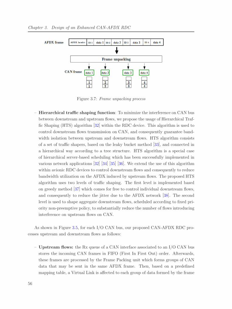
Chapter 3. Design of an Enhanced CAN-AFDX RDC
Figure 3.7: Frame unpacking process
– Hierarchical traffic shaping function: To minimize the interference on CAN bus
between downstream and upstream flows, we propose the usage of Hierarchical Traf-
fic Shaping (HTS) algorithm [32] within the RDC device. This algorithm is used to
control downstream flows transmission on CAN, and consequently guarantee band-
width isolation between upstream and downstream flows. HTS algorithm consists
of a set of traffic shapers, based on the leaky bucket method [33], and connected in
a hierarchical way according to a tree structure. HTS algorithm is a special case
of hierarchical server-based scheduling which has been successfully implemented in
various network applications [32] [34] [35] [36]. We extend the use of this algorithm
within avionic RDC devices to control downstream flows and consequently to reduce
bandwidth utilization on the AFDX induced by upstream flows. The proposed HTS
algorithm uses two levels of traffic shaping. The first level is implemented based
on greedy method [37] which comes for free to control individual downstream flows,
and consequently to reduce the jitter due to the AFDX network [38]. The second
level is used to shape aggregate downstream flows, scheduled according to fixed pri-
ority non-preemptive policy, to substantially reduce the number of flows introducing
interference on upstream flows on CAN.
As shown in Figure 3.5, for each I/O CAN bus, our proposed CAN-AFDX RDC pro-
cesses upstream and downstream flows as follows:
– Upstream flows: the Rx queue of a CAN interface associated to an I/O CAN bus
stores the incoming CAN frames in FIFO (First In First Out) order. Afterwards,
these frames are processed by the Frame Packing unit which forms groups of CAN
data that may be sent in the same AFDX frame. Then, based on a predefined
mapping table, a Virtual Link is affected to each group of data formed by the frame
56

3.3. Frame Packing Strategies
packing unit to ensure its delivery to the AFDX end-systems. As we can see in
Figure 3.5, flows from different I/O CAN buses can not be packed together. Indeed,
as partitioning mechanism is implemented to isolate upstream flows coming from
different CAN buses, the interaction between different upstream flows is limited to
the AFDX interface which handles contention between VLs from different partitions.
– Downstream flows: For downstream flows, the I/O processing unit moves frames
from the AFDX Rx interface to the corresponding partition, based on the forwarding
table. Then, these received frames are processed within the unpacking frame unit.
This latter extracts one or many elementary data from the same AFDX frame de-
pending on the data packing performed within the initial AFDX source. Afterwards,
based on a mapping table, CAN identifiers are defined and CAN data are encapsu-
lated with the appropriate CAN headers to form CAN frames. HTS mechanism is
implemented in the RDC device to eliminate the jitter due to the AFDX network,
and minimize interference on CAN buses between upstream and downstream flows.
3.3 Frame Packing Strategies
In this section, we first review main related work to frame packing technique. Then,
we introduce two frame packing strategies for the CAN-AFDX RDC device.
3.3.1 Related Work
In the literature, several frame packing strategies were introduced for different appli-
cations, and can be organized into two classes:
– Dynamic frame packing: the groups of data messages to pack within the same
AFDX frame are not fixed a priori. A specific criterion for grouping data on the fly
during execution time is defined, such as the number of messages to pack;
– Static frame packing: the groups of data messages are fixed offline and do not
change during system execution.
In [28], a dynamic frame packing approach has been proposed within CAN-Ethernet
bridges. It consists in fixing the number of elementary CAN packets in each transmitted
57

Chapter 3. Design of an Enhanced CAN-AFDX RDC
Ethernet frame to reduce the induced Ethernet overhead by CAN flows. Using simulation,
obtained communication latencies showed significant overhead savings on the Ethernet
network, compared to using basic bridges with a naive (1:1) strategy for frames conver-
sion between CAN and Ethernet networks. However, no analytical proof was provided
concerning the verification of schedulability constraints as required for hard real-time ap-
plications. Another interesting dynamic packing strategy was proposed in [39] to construct
network frames from applications data for non real-time networks. This latter strategy is
based on a predefined frame’s filling level. Hence, messages are packed in the same frame
until reaching the filling level. This approach could be efficient to reduce the overhead
and to minimize the bandwidth consumption for non real-time applications. However, for
real-time communication with hard constraints, this approach can lead to a poor tempo-
ral behavior since the schedulability issue was not integrated in the frame packing design
phase.
Static packing approaches have been introduced and studied for different applications,
especially for automotive communications in [14] [15] [16] and for avionics communications
in [12]. In automotive networks [14] [15], authors considered a communication network
based on CAN protocol and addressed the problem of building CAN frames to support a
set of data from applications hosted by an Electronic Controller Unit (ECU), i.e., an auto-
motive terminal. Various algorithms were proposed to select the best static frame packing
which minimizes the load on CAN bus while meeting the timing constraints. Obtained
results have shown the efficiency of static frame packing in saving network resources, es-
pecially in terms of bandwidth utilization. However, the introduced packing approaches
in [14] and [15] assumed a high synchronization level between their applications within
the same ECU. This fact makes the application of these approaches complex in our case
where data incoming to the RDC device are serialized after their transmission on the
source network, i.e., a CAN bus for our CAN-AFDX case study.
In [16], authors introduced a static frame packing algorithm for automotive ECUs in a
multi-cluster automotive architecture based on two different buses: a time-triggered and
an event-triggered. Moreover, a gateway is used to support inter-buses communication.
Authors used a static frame packing strategy to affect signals, i.e., elementary applications
messages, to periodic frames that need to be transmitted on the communication network.
Obtained results showed the enhancements of system’s schedulability due to frame pack-
ing strategy within the ECUs. However, The considered gateway performs a simple (1:1)
conversion strategy, and tuning the frame packing strategy parameters is a complex task.
In avionics context, a static frame packing scheme was introduced in [12] to be applied
58

3.3. Frame Packing Strategies
inside AFDX end-systems to map applications data into AFDX VLs. An algorithm to
select the best frame packing in terms of bandwidth utilization was introduced. However,
this algorithm did not integrate schedulability constraints to discard non-feasible configu-
rations. Moreover, the proposed frame packing needs a high synchronization level between
applications hosted by the same AFDX end-system. This assumption is not verified in
our case since data are serialized on the source network before achieving the RDC device.
This fact makes the applicability of this strategy complex in our case.
Hence, some static frame packing approaches were proposed in the literature for both
automotive and avionics applications. However, these researches addressed maily the
problem of affecting elementary applications data to network frames within source nodes,
and not within interconnection devices.
In the rest of this section, we present two frame packing strategies integrated in our
enhanced RDC device. The first one is dynamic, called Fixed Waiting Time (FWT), while
the second one is static, called Messages Set Partitioning (MSP).
3.3.2 Dynamic Strategy: FWT
This strategy is based on a waiting timer, as illustrated in Figure 3.8. This timer is
started at the end of reception of the first CAN message at the packing queue, and it
allows the accumulation of many CAN messages at the RDC CAN interface. Then, when
the timer expires, the gathered data messages will be sent within the same AFDX frame.
Afterwards, each AFDX frame is transmitted into one of the virtual links defined in the
RDC to support the upstream flows, i.e. sensors flows.
Figure 3.8: FWT frame packing strategy for upstream flows
59

Chapter 3. Design of an Enhanced CAN-AFDX RDC
3.3.3 Static Strategy: MSP
The MSP strategy consists in defining off-line a partition of CAN messages set, where
each obtained subset represents the composition of an AFDX frame, as illustrated in Fig-
ure 3.9. An RDC device implementing MSP packing strategy proceeds as following. First,
the received CAN messages are queued in the input port of the RDC device. Then, based
on a static mapping table, each CAN frame is relayed to its associated output queue. The
frame packing is synchronized with the reception of the most urgent CAN frame among
each defined sub-partition. A timeout could be implemented to avoid losing all the ac-
cumulated messages in case of non-reception of the most urgent one. Finally, the output
AFDX VLs will be multiplexed in the output port of the RDC device according to FIFO
policy and then transmitted on the AFDX network.
Figure 3.9: MSP frame packing strategy on upstream flows
3.4 Data Mapping & Formatting
To set up a frame packing and unpacking units in the RDC device, two important
issues have to be considered: data mapping and frame formatting.
3.4.1 Data Mapping
To integrate the frame packing process with enhanced RDC device, the static mapping
is no longer based on associating one VL ID for each CAN ID, but one VL to multiple
CAN IDs unlike the current RDC device. This mapping is illustrated in Table 3.10, where
seven CAN messages are affected to three VLs. For each frame packing strategy, the ade-
quate mapping table should be defined and configured to respect the different addressing
schemes.
60

3.4. Data Mapping & Formatting
Figure 3.10: Mapping table for enhanced RDC device
3.4.2 Frame Formatting
The frame packing process in the CAN-AFDX RDC device consists in including sev-
eral data in the payload of one AFDX frame. This fact requires the definition of adequate
AFDX frame structures, which may depend on the implemented frame packing strategy.
To define the most accurate AFDX frame structure for each considered frame packing
strategy, we follow the guidelines provided by the ARINC 664 standard [1] for formatting
AFDX frame payload. A payload corresponds to one or several elementary data and it
is created and received at the application layer. We consider the concept of Functional
Data set (FDS), introduced in the standard ARINC 664 [1]. As shown in Figure 3.11, an
FDS allows grouping multiple data in the same AFDX frame and consists of two fields:
(i) Data Sets (DS) that can contain several data primitives (e.g., Float, Integer, Boolean);
(ii) Functional Status Set (FSS) which is a 4 Bytes field to encode the correctness and
the status of at maximum 4 Data Sets. Several FDS data sets may be used to organise
data included in the AFDX payload.
In order to keep communication overhead as low as possible in the AFDX payload
structure, we chose the structure of Figure 3.12. One FSD is defined which is composed
of one DS containing all the data messages to send within the AFDX frame and one FSS
encoding the status of the supported data set.
Furthermore, the standard ARINC 664 defines two types of frame structures:
– Explicit structure: The frame format includes information allowing the desti-
nation of the frame to decode its payload. The structure includes identifiers to
explicitly identify each elementary data encoded in the frame, and length parameter
to define how long the structure is. An explicit formatting structure is shown in Fig-
ure 3.13: one identifier of 1 byte per data type is used for data identification, and the
number and order of elementary data can vary according to the maximum frame size.
61

Chapter 3. Design of an Enhanced CAN-AFDX RDC
Figure 3.11: Structure of AFDX payload (ARINC 664)
Figure 3.12: Chosen AFDX payload structure
– Implicit structure: Unlike the explicit structure, the frame in this case contains
only elementary data without explicit identifiers. Then, the destination application
will interpret correctly the frame format according to the identifier of the reception
AFDX port. This concept is common in the Internet world with the Well Known
Service (WKS) concept. For example, the File Transfer Protocol (FTP) service is
available on port 21. In a similar way, we can affect to the AFDX port 6 a struc-
ture containing pressure measurement encoded on 8 bytes, followed by temperature
measurement encoded on 4 bytes.
62

3.4. Data Mapping & Formatting
Figure 3.13: Explicit AFDX frame structure
Figure 3.14: Implicit AFDX frame structure
An implicit structure is shown in Figure 3.14 where the frame formats are affected to
port numbers. For each destination port receiving an AFDX frame, the correspond-
ing structure defines the maximum size of the AFDX frame, and the elementary data
fields in a predefined order where each data has a specific type and size. Padding
may be used in the source to keep the same structure of the AFDX frame between
successive transmissions, and to allow destinations to correctly decode included data.
The information about frame structure is shared between senders and receivers.
63

Chapter 3. Design of an Enhanced CAN-AFDX RDC
The appropriate formatting structure which minimizes the induced communication
overhead while guaranteeing correct identification of data, should be selected during the
network design. This choice will mainly depend on the avionics applications and the
knowledge of the AFDX frames composition during execution time. In our case, this
choice depends also on the frame packing strategy. Hence, the frame structure is chosen
as follows:
– Under FWT: we do not know a priori the set of data to pack in each AFDX frame
since packing is done on-the-fly according to the waiting time parameter. Hence,
the explicit structure is considered as more adequate under FWT packing strategy.
Then, the only parameter to fix in this case is the maximum AFDX frame size, which
is generally the maximum size of all possible resulting AFDX frames under FWT
packing strategy. Thus, we compute the worst-case scenario in terms of gathered
data size during the waiting time to define payload size of the explicit structure of
AFDX frames.
– Under MSP: the composition of the AFDX frames is fixed and is known a pri-
ori. Therefore, using an implicit structure is more adequate in this case to identify
packed data into the AFDX frames.
3.5 Traffic Shaping Mechanism
In this section, we first review the main related work to traffic shaping mechanism.
Then, we introduce a traffic shaping technique, called Hierarchical Traffic Shaping (HTS),
adapted to our CAN-AFDX RDC device to isolate upstream and downstream flows and
control contention between them on I/O CAN buses.
3.5.1 Related Work
Traffic shaping is a traffic management technique which consists in delaying some
packets to be conform with a desired traffic profile. It is a widely used technique in
communication networks in general, and especially in real-time networks. It is used to
guarantee performances and to improve latencies by bounding packets interference.
The Hierarchical Traffic Shaping (HTS) is a part of general Hierarchical Server-Based
64

3.5. Traffic Shaping Mechanism
(HSB) Scheduling where each traffic shaper in the hierarchy structure is considered as a
server which will bound the traffic burstiness sent within a limited time window. HSB
scheduling is a common approach that has been used in many network applications to
control interference between various traffic classes with different real-time requirements,
i.e., Soft Real-Time (SRT) and Hard Real-Time (HRT) traffic. Concerning industrial ap-
plication and especially Real-Time Ethernet, one of the most relevant approaches based
on HSB framework to guarantee a dynamic adaptation of servers was proposed in [36].
The authors presented a multi-level HSB architecture for Ethernet, implemented on com-
mercial switches and based on FTT-SE (Flexible Time Triggered Switched Ethernet)
paradigm [40]. Schedulability analysis was detailed and validated using experimentation.
This approach is efficient in dynamic environment, and typically open networks. However,
it assumes that servers parameters verify a priori traffic temporal constraints.
In automotive applications, various approaches based on traffic shaping and HSB
scheduling were proposed to improve CAN bus performances. In [38], traffic shaping
algorithm based on leaky bucket method, and particularly greedy method [37], was in-
tegrated within gateways to reduce the jitter on the destination network and improve
the schedulability of lower priority messages. However, this approach is considered as a
limited form of HTS approach implementing only one level of traffic shapers to control in-
dividual input messages. In [35], HSB scheduler, based on Earliest Deadline First (EDF)
algorithm, was detailed to use CAN in a more flexible way compared to native CAN. This
approach improved bandwidth isolation among aperiodic traffic and was validated using
simulation. However, no analytical approach was proposed to provide worst-case response
times of messages and to guarantee messages schedulability.
In avionics application, traffic shaping is integrated in AFDX end-systems to guarantee
a reserved bandwidth for each application and is standardized as Virtual Link concept.
This approach guarantees bandwidth isolation between traffic flows and improves the pre-
dictability of the AFDX network. In our case, we extend this approach by implementing
HTS scheduling within RDC devices to interconnect the backbone AFDX with I/O CAN
buses. The main idea is to minimize the interference due to downstream flows on the
transmission of upstream flows on CAN, and consequently the WCRTs on CAN of up-
stream flows. This will favor frame packing mechanism for upstream frames within RDC
device, and thus will reduce bandwidth utilization on the AFDX.
Our proposal consists of two traffic shaping levels and a root server to implement
native CAN scheduler. The idea of the first level of traffic shapers is very similar to the
65

Chapter 3. Design of an Enhanced CAN-AFDX RDC
one detailed in [38] where we consider greedy method, which does not increase maximum
end-to-end delays as proved in [37], and induced jitter by the AFDX network. However,
we extend this implementation by adding a second level of traffic shapers to substan-
tially reduce the number of flows introducing interference on upstream flows on CAN.
The schedulability analysis of upstream and downstream flows is proved and validated
through a realistic avionic case study. Furthermore, unlike [36], a tuning process of the
HTS parameters is proposed to minimize as much as possible bandwidth utilization on
the AFDX, while guaranteeing at the same time upstream and downstream flows require-
ments.
3.5.2 HTS Algorithm
The HTS mechanism is based on a set of traffic shapers and servers connected in a
tree structure and defined in a static manner a priori, as shown in Figure 3.15. This latter
is organized into three levels: leaf, inner and root.
Figure 3.15: Hierarchical Traffic Shaping structure
66

3.6. Conclusion
– Leaf traffic shapers: are implemented to control the flow of received packets from
the AFDX network. They are based on greedy method [8]. A greedy shaper is a
special traffic shaper, that not only ensures an output stream that conforms to a
given traffic specification, but that also guarantees that no packets get delayed any
longer than necessary. In our case, leaf shapers ensures the same minimal inter-
arrival time as in AFDX sources for each downstream flow. Hence, do not increase
maximum end-to-end delays, however, they reduce efficiently the observed jitter in
the RDC device. This fact enhances lower priority messages schedulability on CAN
[9].
– Inner traffic shapers: each one is based on leaky bucket method to shape aggre-
gate downstream flows of outgoing packets from leaf shapers after being classified
and scheduled according to a fixed priority non-preemptive policy. The aim of these
shapers is to substantially reduce the number of flows introducing interference on
upstream flows, and to guarantee bandwidth isolation on CAN. One or many inner
traffic shapers can be implemented depending on the incoming traffic rate. Indeed,
shaping all the incoming flows using the same inner traffic shaper will induce small
inter-arrival time between packets at the output, and consequently important in-
terference with upstream flows. The tuning process of these inner shapers will be
detailed in next chapters.
– The root server implements simply fixed priority non-preemptive scheduling which
represents the CAN native behavior. All the packets will be multiplexed at the root
server according to their corresponding priorities.
3.6 Conclusion
In this chapter, we presented an enhanced RDC device which is capable of: (i) con-
necting multiple I/O CAN networks to AFDX; (ii) saving AFDX bandwidth by reducing
communication overheads induced by the RDC. Compared to the currently used RDC,
our proposed RDC implements a set of additional functions: (i) frame packing based on
dynamic or static strategy; (ii) frame unpacking; (iii) Hierarchical Traffic Shaping (HTS).
The upstream flows, i.e., flows sent from CAN to AFDX, are processed by the frame
packing strategy in the RDC; while the downstream flows, i.e., flows sent from CAN to
AFDX, are first unpacked to extract elementary CAN data, then they are processed by
the HTS unit. Furthermore, a partitioning process, ARINC 653-compliant, is used in the
67

Chapter 3. Design of an Enhanced CAN-AFDX RDC
RDC to isolate communication from different I/O CAN buses. A partition in the RDC
is affected to each I/O CAN bus connected to the AFDX network. This choice reduces
the number of required RDC hardware units, and thus reduces the system weight and cost.
The proposed RDC device presents several advantages such as modularity, configura-
bility and resource management efficiency. However, introduced functions imply addi-
tional complexity in the performance analysis and RDC configuration task. As the RDC
device inherits from the avionics system requirements, we have to prove that it meets
real-time requirements. In the next chapter, we will introduce adequate timing analysis
approach to validate the real-time behaviour of our proposed RDC device, while enhanc-
ing network resource savings.
68

Chapter 4
Modeling and Timing Analysis of
the Enhanced RDC
In this chapter, we first model the CAN-AFDX network interconnected using our en-
hanced RDC device and the supported data flows. Afterwards, a timing analysis method
is proposed and detailed to verify the system schedulability under different RDC’s con-
figurations. A performance evaluation through a small scale CAN-AFDX network is then
provided.
4.1 CAN-AFDX RDC Modeling
Figure 4.1: CAN-AFDX network architecture
As shown in Figure 4.1, the traffic supported by the RDC device can be organized
into two types of flows: (i) upstream flows received from sensors connected to CAN bus
and destined to calculators on AFDX; (ii) downstream flows received from calculators
connected to AFDX and destined to actuators connected to CAN bus. We consider Sup
and Sdown for upstream and downstream flow sets, respectively. For each stream flow
m ∈ Sup ∪ Sdown, we associate four characteristics {Tm, Lm, Dlm, Pm} which represent the
69

Chapter 4. Modeling and Timing Analysis of the Enhanced RDC
period, maximum payload, deadline and priority on CAN bus, respectively. We consider
a strict order of CAN priorities, i.e. for any two messages mk and mj , Pmk< Pmj
means
that message mk has higher priority than mj .
When upstream and downstream flows cross the RDC device, they are processed as
follows:
– Upstream flows: as shown in Figure 4.2, the RDC device maps CAN messages
set Sup onto AFDX VLs set to support the upstream flows on AFDX network.
This mapping process is called VLs allocation. To check the network temporal con-
straints, the allocated VLs need to be completely characterized. The VLs allocation
is detailed for each proposed frame packing strategy, i.e., FWT and MSP, in Section
4.1.1;
Figure 4.2: Upstream flows modeling from end-to-end
– Downstream flows: as shown in Figure 4.3, the RDC device will first extract the
CAN messages set Sdown from the AFDX VLs. Then, the obtained CAN messages
are processed by the set of shapers in the HTS structure. To prove the network
temporal guarantees, these shapers have to be completely characterized. The map-
ping of downstream flows Sdown onto the shapers of the HTS structure is detailed
in Section 4.1.2.
Figure 4.3: Downstream flows modeling from end-to-end
70

4.1. CAN-AFDX RDC Modeling
4.1.1 Frame Packing Strategies Modeling
The frame packing process consists in building a set of AFDX VLs V = {v1, v2, ..., vm}to define the output traffic from the RDC to the AFDX network, knowing the set of
CAN-messages M = {m1, m2, ..., mn} at the input.
Figure 4.4: Example of CAN messages mapping onto AFDX VLs
As we can see through the example of Figure 4.4, after the frame packing process, each
AFDX frame fi within the VL vi ∈ V will contain a subset of CAN messages M(vi) ⊂M .
This subset of messages which can be static under MSP strategy, i.e., does not change
over successive transmissions, or dynamic under FWT strategy, i.e., may vary from a
transmission to another. Each VL vi is characterized by {BAGi,MFSi, Dli, DESiAFDX}
which represent the bandwidth allocation gap, the maximum frame size, the deadline and
the set of AFDX end-system destinations, respectively. These characteristics will clearly
depend on the implemented frame packing strategy in the RDC, and will be developed in
the rest of this section.
4.1.1.1 FWT Strategy
For an RDC device implementing the FWT strategy with a waiting timer ∆, we define
a set of AFDX VLs to support the AFDX frames resulting from FWT packing process.
The number of VLs is defined considering that the RDC can forward as much AFDX
frames as timer ∆ occurrences during the smallest period of the CAN messages set M .
Hence, we define the number of VLs to support CAN messages under FWT strategy as
71

Chapter 4. Modeling and Timing Analysis of the Enhanced RDC
follows:
Nvls(∆) = Card(V ) =
⌈minmj∈M Tj
∆
⌉(4.1)
In the worst-case scenario, any defined virtual link may support the most urgent CAN
data and may include the maximum number of elementary CAN data accumulated during
the FWT packing process. Hence, the allocated VLs V to the CAN traffic under FWT
strategy which cover the worst-case scenario are considered as identical in terms of their
composing elementary data, and their characteristics are defined as following.
For any vi ∈ V ,
– BAGi: since any allocated VL vi needs to transmit the message having the smallest
period within the messages set M , we define the BAG as the closest value in power
of 2 to the smallest period of messages in M :
BAGi = 2k, k =
⌊log(minmj∈MTj)
log(2)
⌋(4.2)
– MFSi: is considered as the sum of all data payloads in the messages set M and the
induced overhead imposed by the AFDX structure. Padding may be used to guar-
antee a minimum AFDX frame size of 84 bytes (IFG (Inter Frame Gap) included).
The largest AFDX frame generated by the RDC depends on the waiting time ∆.
According to the explicit structure detailed in the previous chapter, a bound on the
maximal frame size (in bits) is as follows:
MFSi = max(84 ∗ 8,min(Si,∆ ∗
8
17∗ 106) + (67 +Nlb(∆)) ∗ 8
)(4.3)
where,
– Si is the sum of all data payloads in M (in bits);
– ∆∗ 8
17∗106 is the maximal payload (in bits) that can be accumulated in the RDC
during ∆. The typical CAN parameters are integrated where 8 bytes correspond
to the maximum CAN payload size, and 17 bytes the size of a maximum frame
size including payload and CAN protocol overhead and a transmission capacity
of 106Mbps;
72

4.1. CAN-AFDX RDC Modeling
– (67+Nlb(∆))∗8 is the overhead (in bits) imposed by the AFDX explicit structure,
where Nlb(∆) is the maximal number of CAN identifiers received during ∆;
– Padding may be used to ensure a minimum AFDX frame size of 84 bytes.
– Dli: is the relative deadline of the obtained AFDX frame. This relative deadline
will be detailed in Section 4.2.
– DESiAFDX : since any VL vi in V can include any CAN message in M , then vi can
be received by any AFDX end-system that initially consumes at least one of these
data. Therefore, DESiAFDX is as follows:
DESiAFDX = ∪mj∈MDESj
AFDX (4.4)
An example of AFDX VLs allocation under FWT strategy is shown in Figure 4.5. In
this example, a set of 4 CAN messages is mapped onto 2 AFDX VLs. The choice of VL
to support packed data is done during the execution time among VLs 1 and 2.
Figure 4.5: Example of AFDX VLs allocation under FWT strategy
4.1.1.2 MSP Strategy
The MSP strategy for CAN-AFDX RDC is defined using a partitioning process of
CAN messages set M . Each AFDX VL vi ∈ V consists of a sub-set M(vi) of CAN mes-
73

Chapter 4. Modeling and Timing Analysis of the Enhanced RDC
sages obtained after the partitioning process and it is characterized as follows:
– BAGi: unlike FWT strategy, under the MSP strategy the subset M(vi) is fixed.
Therefore, for a AFDX VL vi the BAG is computed as follows:
BAGi = 2k, k =
⌊log(minmj∈M(vi)Tj)
log(2)
⌋(4.5)
– MFSi: unlike FWT, under MSP strategy an implicit AFDX frame structure is used
and the sub-set of CAN messages M(vi) to pack is known a priori. Therefore, an
accurate MFS (in bits) for AFDX VL vi is computed as follows:
MFSi = max(84,
∑
mj∈M(vi)
Lj + 67)∗ 8 (4.6)
– Dli: is the relative deadline of the obtained AFDX frame which depends on its
associated CAN-messages subset M(vi). Unlike FWT strategy, under MSP strategy
only the impact of CAN messages in M(vi) needs to be taken into account instead
of all CAN messages set M with FWT;
– DESiAFDX : under MSP strategy, the sub-set M(vi) is known a priori. Therefore,
the set of AFDX destination end-systems is more accurate than under FWT:
DESiAFDX = ∪mj∈M(vi)DESj (4.7)
An example of AFDX VLs allocation under MSP strategy is illustrated in Figure 4.6.
In this example, a set of 4 CAN messages is mapped onto 2 AFDX VLs. VL 1 supports
the successive transmission of frames containing messages 1 and 3, whereas VL 2 supports
the successive transmission of frames 2 and 4.
74

4.1. CAN-AFDX RDC Modeling
Figure 4.6: Example of AFDX VLs allocation under MSP strategy
4.1.2 HTS Mechanism Modeling
The HTS is used to manage downstream flows to minimize interference with upstream
flows on CAN. Each leaf traffic shaper is applied for only one type of downstream flow
and consequently admits the same period and authorized maximum payload than its as-
sociated flow. However, an inner traffic shaper is applied to a group of outgoing flows
from leaf shapers. Then, each inner shaper sh in the set of inner shapers Shinner, applied
for a set of downstream flows Ssh, is characterized by {Tsh, Lsh, Psh}, where:
– Tsh is the period. This value is comprised between T minsh and T maxsh depending
on the characteristics of Ssh. To support the aggregate flow rate, T maxsh is at most
equal to 1∑i∈Ssh
1Ti
. Furthermore, to avoid overflowing the CAN bus, we consider
that T minsh is at least equal to 1ms, which is an arbitrary choice that integrates
CAN transmission capacity and typical production periods of CAN sources. If1∑
i∈Ssh
1Ti
> 1ms, than this configuration is possible; else we should investigate other
HTS configurations;
– Lsh is the maximum payload size where Lsh = maxi∈Ssh
Li;
– Psh is the associated priority to the inner shaper. This value depends on the consid-
ered communication way and is equal to P minsh or P maxsh. To cover the worst-case
from the downstream flows point of view, this priority is considered as the lowest
75

Chapter 4. Modeling and Timing Analysis of the Enhanced RDC
priority among all its input downstream flows set, and Psh = P maxsh = maxi∈Ssh
Pi.
However, the worst-case from the upstream point of view corresponds to considering
the highest priority among all its input downstream flows set and Psh = P minsh =
mini∈Ssh
Pi.
4.2 Timing Analysis
In this section, we first introduce a schedulability test based on end-to-end latencies
to analyze the timing guarantees offered by our enhanced RDC to the crossed flows. Af-
terwards, an adequate timing analysis is provided to compute end-to-end latencies and
evaluate the timing performance of the RDC.
4.2.1 Sufficient Schedulability Test
For avionics embedded applications, it is essential that the communication network ful-
fills certification requirements, e.g. predictable behavior under hard real-time constraints
and temporal deadline guarantees. The use of a frame packing process and traffic shaping
within the RDC may increase communication latencies and real-time constraints have to
be checked. To deal with the worst-case performance analysis of such networks, we con-
sider as a metric the worst-case end-to-end delay that will be compared to the temporal
deadline for each frame.
Figure 4.7: End-to-end delay metric definition
The end-to-end delay deed(mj) of each CAN message mj ∈M(vi), where M(vi) is the
subset of CAN-messages associated with the VL vi ∈ V , consists of three parts as shown
76

4.2. Timing Analysis
in Figure 4.7:
– dCAN(mj): is the maximal response time of a CAN frame. A schedulability analysis
for native CAN bus has been introduced in [11], where the CAN bus is modeled as
a static priority non-preemptive scheduler. This analysis will be adapted in the case
where the HTS mechanism is applied in the RDC.
– dRDC(mj): is the maximal duration the message mj might be delayed in the RDC.
This delay depends mainly on the implemented frame packing strategy in the RDC
device for upstream flows, and on the HTS mechanism implemented for downstream
flows. For upstream flows, this delay is the sum of: (i) a technological latency,
denoted by ǫ, which is due to payload extraction/encapsulation and reading the
mapping table; (ii) waiting time in the RDC between the reception instant of the
CAN message and the transmission instant of its associated AFDX frame, denoted
by WT (mj), then
dRDC(mj) = ǫ+WT (mj) (4.8)
In this section, we will provide bounds on the RDC traversal latency for both up-
stream and downstream flows.
– dAFDX(vi): is the upper bound on the delay experienced by the AFDX VL including
mj . Delay bounds computation for the AFDX network, based on Network Calculus
formalism, has been introduced in [17]. The tool WoPANets presented in [6] and
based on Network Calculus formalism, will be used throughout this work to analyze
AFDX delay bounds (see Appendix A for more details about the Network Calculus
concepts and WoPANets tool).
The proposed schedulability test is as follows:
∀ vi ∈ V , ∀ mj ∈M(vi),
dCAN(mj) + dRDC(mj) + dAFDX(vi) ≤ Dlj (4.9)
77

Chapter 4. Modeling and Timing Analysis of the Enhanced RDC
4.2.2 Timing Analysis for Upstream Flows
First, we provide a method to compute a bound on RDC traversal delay dRDC(m). Af-
terwards, we provide a method to compute a bound on worst-case response time on CAN
bus dCAN(m). The AFDX delay bound dAFDX is computed using WoPANets tool given
the set of allocated VLs obtained according to the implemented frame packing strategy,
as provided in Section 4.1.1.
4.2.2.1 RDC Traversal Delay Computation
The RDC device delay imposed to upstream flows is due to the frame packing unit.
Under FWT strategy, the worst-case waiting time in the RDC is equal to ∆. As shown
in Figure 4.8, this occurs when a CAN message is not completely received at the FWT
packing queue before the expiration of an already started timer of duration ∆. In this
case, the received CAN message has to be transmitted within the next AFDX frame which
is built after the expiration of a timer of duration ∆.
Figure 4.8: Worst-case waiting time under FWT strategy
Hence, a bound on the waiting time for message mj in the RDC device under FWT
strategy is given as follows:
WT (mj) = ∆ (4.10)
Under MSP packing strategy, the worst-case waiting time of a CAN-message mj ∈M(vi) \ {ms}, where ms is the message with the smallest period, occurs when it arrives
78

4.2. Timing Analysis
immediately after the end of ms reception in the RDC. In this case, the message mj has
to wait for the next reception of ms to be packed in the same AFDX frame, as illustrated
in Figure 4.9. Therefore, an upper bound of the waiting time in the RDC ofmj ∈M(vi) is:
WT (mj) =
{0 if j = s
Ts + dCAN(ms) otherwise(4.11)
Figure 4.9: Worst-case waiting time under MSP strategy
4.2.2.2 CAN Worst Case Response Time Computation
In [11], the CAN bus was modeled as a static priority non-preemptive scheduler
and the Worst Case Response Time (WCRT) for a message m was provided:
dCAN(m) = Rm
= maxq=0..Qm−1
Rm(q) (4.12)
where Qm is the number of instances of message m that become ready to transmission
before the end of the busy period relative to m, and Rm(q) is the WCRT of instance q of
message m. Rm(q) is given by:
Rm(q) = Cm + Jm + wm(q)− qTm (4.13)
where,
– The transmission time Cm, corresponding to the longest time that the message can
take to be transmitted;
79

Chapter 4. Modeling and Timing Analysis of the Enhanced RDC
– The queuing jitter Jm, corresponding to the longest time between the initiating
event and the message being queued, ready to be transmitted on the bus;
– The queuing delay wm(q) , corresponding to the longest time that the instance q of
messagem can remain in the CAN controller queue, before commencing transmission
on the bus.
– Tm is the period of message m.
wm(q) is computed using the following iterative expression:
wn+1m (q) = Bm + qCm +
∑
k∈hp(m)
⌈wn
m(q) + Jk + τbitTk
⌉∗ Ck (4.14)
where hp(m) corresponds to the set of messages with priority higher than m, τbit
the transmission time of one bit and Bm the maximum blocking time due to the set of
messages with lower priority than m, denoted by lp(m). The recurrence relation starts
with a value of w0m(q) = Bm + qCm, and ends when wn
m(q) = wn+1m (q), or when Rm(q) =
Cm + Jm +wn+1m (q)− qTm > Dlm in which case the message is unschedulable. For values
of q > 0 an efficient starting value is given by w0m(q) = wm(q − 1) + Cm. Bm is given by:
Bm = maxk∈lp(m)
Ck (4.15)
The number of instances that need to be examined Qm is given by:
Qm =
⌈tm + Jm
Tm
⌉(4.16)
where tm corresponds to the length of the priority level-m busy period is given by
the following recurrence relation, starting with an initial value of tm = Cm, and finishing
when tn+1m = tnm:
tn+1m = Bm +
∑
k∈hep(m)
⌈tnm + Jk
Tk
⌉∗ Ck (4.17)
hep(m) is the set of messages with priority higher or equal to m.
The response time computed using equations 4.12 to 4.17 corresponds to the exact
WCRT on CAN. However, it may induce a high computing complexity since it potentially
requires the computation of multiple response times for each CAN message. In [11],
authors presented a simpler but more pessimistic schedulability test which computes an
upper bound on the WCRT on CAN, which is only valid for CAN messages with
80

4.2. Timing Analysis
deadlines less or equal to periods. An upper bound on WCRT on CAN for message
m can be thus given by:
dCAN(m) = Cm + wm + Jm (4.18)
where, wm is an upper bound on the queueing delay of any instance q of message m,
which is obtained using the following iterative expression:
wn+1m = max(Bm, Cm) +
∑
k∈hp(m)
⌈wn
m + Jk + τbitTk
⌉∗ Ck (4.19)
We denote by lep(m) the set of flows with priority lower of equal to m, then, 4.19 can
be written as follows:
wn+1m = max
k∈lep(m)(Ck) +
∑
k∈hp(m)
⌈wn
m + Jk + τbitTk
⌉∗ Ck (4.20)
To check the schedulability of message m on CAN, we start with an initial value
w0(m) = Cm and continue until obtaining one of these two situations: (i) wn+1(m) +
Cm + Jm > Dlm, then stop but no conclusion on the schedulability of message m; (ii)
wn+1(m) = wn(m), then stop and conclude m is schedulable with an upper bound on its
WCRT of wm + Cm + Jm.
In order to compute the exact WCRT on CAN using equations 4.12 to 4.17, we define
for an upstream flow m the set of messages hp(m) and lp(m) required for this timing
analysis:
– hp(m) = {k ∈ Sup ∪ Shinner / Pk < Pm}: set of messages with priorities higher
than m among upstream flows and the set of inner shapers in HTS structure by
considering P minsh for each inner shaper sh ∈ Shinner;
– lp(m) = {j ∈ Sup ∪ Shinner / Pk > Pm}: set of messages with priorities lower or
equal than m among upstream flows and the set of inner shapers in the HTS struc-
ture by considering P minsh for each inner shaper sh ∈ Shinner.
To apply the sufficient schedulability test using equation 4.18 and 4.19, we define for
an upstream flowm the set of messages hp(m) and lep(m) required for this timing analysis:
81

Chapter 4. Modeling and Timing Analysis of the Enhanced RDC
– hp(m) = {k ∈ Sup ∪ Shinner / Pk < Pm}: set of messages with priorities higher
than m among upstream flows and the set of inner shapers in HTS structure by
considering P minsh for each inner shaper sh ∈ Shinner;
– lep(m) = {j ∈ Sup ∪ Shinner / Pk ≥ Pm}: set of messages with priorities lower
or equal than m among upstream flows and the set of inner shapers in the HTS
structure by considering P maxsh for each inner shaper sh ∈ Shinner.
In Section 4.2.2.3, we conduct a comparison between the upper bound on the WCRT
on CAN bus and the exact WCRT to evaluate the degree of pessimism of the upper bound.
The schedulability test 4.9 can be verified for each message m using equation 4.10, 4.11,
4.12 (or 4.18 under the assumption that the deadline of a message is equal to its period)
and the obtained AFDX delay bounds using WoPANets tool.
4.2.2.3 CAN analysis: upper bound vs exact WCRT
To illustrate the proposed timing analysis on CAN and assess the pessimism of the
upper bound on the WCRT on CAN, we consider the following examples of flows on CAN:
– Example 1: we consider three messages corresponding to the example of Table 3
in [11], which was used to highlight the flaw in the analysis introduced by Tindell
and al. in [25], as described in Table 4.1. The CAN message’s payload leading to a
transmission time of 1 ms is equal to 116 bytes, which largely exceeds the maximum
payload of 8 bytes allowed by CAN and the deadline of each message is equal to its
production period. Even if this traffic is non realistic for a CAN bus, we use it to
compare WCRT and the proposed upper bound on WCRT for CAN-like schedulers.
Table 4.1: Example 1: traffic characterization
Message Priority Period (ms) Tx time (ms) Deadline (ms)
A 1 2.5 1 2.5
B 2 3.5 1 3.5
C 3 3.5 1 3.5
– Example 2: we randomly generate a set of CAN messages with periods in 4,8,16ms
and payloads in the interval [2,8]bytes. We consider several messages sets with a
CAN utilization rate between 15% and 70%. The priorities are assigned to messages
82

4.2. Timing Analysis
such as Pi < Pj if Ti < Tj, i.e. the lower the period of mi is the higher its priority is.
For messages with the same period we arbitrary associated distinct priorities. The
deadline of each CAN message is considered equal to its production period.
To evaluate the pessimism of the upper bound on the WCRT on CAN, for each of the
previous CAN flows examples, we compute the exact WCRT using equation 4.12 and the
upper bound on the WCRT using equation 4.18. Afterwards, we compare the obtained
results and conclude on the degree of pessimism of our schedulability test.
For example 1, the obtained WCRT and upper bound on WCRT on CAN are re-
ported in Table 4.2.
Table 4.2: Example 1: exact WCRT vs upper bound
Message Deadline (ms) WCRT (ms) Upper Bound (ms)
A 2.5 2 2
B 3.5 3 3
C 3.5 3.5 7
The upper bounds obtained for messages A and B are equal to the exact WCRT.
However, for message C we obtain a pessimistic upper bound of 7 ms compared to the
exact WCRT which is equal to 3.5 ms. For this example, the CAN utilization is equal to
97% and messages utilization rates (Cm/Tm) are relatively high, 40% for A and 28% for
B and C.
For example 2, we consider the generated CAN traffic with the utilization rate 70%.
The obtained WCRT and upper bound for each CAN message are reported in Figure
4.10. As can be seen, the obtained upper bounds for CAN messages are equal to the
exact WCRT for all the messages except message 42 where the upper bound is slightly
higher than the exact WCRT. The results obtained for generated CAN messages sets
with low CAN utilization rates show very tight upper bounds. In this case, the number of
instances obtained using Equation 4.17 is equal to 1 and the difference between computed
WCRT and the upper bound is due to considering max(Bm, Cm) (for the upper bound)
instead of max(Bm) (for the exact WCRT).
83

Chapter 4. Modeling and Timing Analysis of the Enhanced RDC
0
2
4
6
8
10
0 5 10 15 20 25 30 35 40 45
WC
RT
/Upp
er B
ound
(ms)
CAN message ID
Upper Bound (ms) Exact WCRT (ms)
Figure 4.10: Comparison between exact WCRT and upper bound (Example 2)
The example 1 shows that under some extreme conditions (a very high CAN load,
high individual utilization rates) the analysis using the upper bound may lead to large
upper bound compared to the exact WCRT. However, for example 2, which represents
a realistic CAN traffic in terms of payload size, periods and CAN bus utilization, the
obtained results showed tight upper bounds on the WCRT. In our study, we consider
realistic CAN traffic with similar properties as those of example 2 and we use the upper
bound on WCRT for timing analysis on CAN bus to simplify the computation.
4.2.3 Timing Analysis for Downstream Flows
Downstream flows are subject to HTS when crossing the RDC device. In this section,
we provide a method to compute a bound on RDC traversal delay, dRDC(m). After-
wards, we provide a method to compute a bound on worst-case response time on CAN
bus dCAN(m).
4.2.3.1 RDC Traversal Delay Computation
The RDC delay dRDC(m) for a downstream flow m is composed of: (i) a technolog-
ical latency, denoted by ǫ due to payload extraction, unpacking and data encapsulation
process; (ii) a blocking time due to the HTS structure, denoted by Bshaper(m). The RDC
delay can be written as follows:
dRDC(m) = ǫ+Bshaper(m) (4.21)
84

4.2. Timing Analysis
For each downstream messagem, first the leaf shaper, based on greedy method, absorbs
the jitter due to AFDX network without increasing the maximal AFDX delay. The impact
of this shaper on end-to-end delay is thus included in the AFDX delay. Furthermore, the
input flows of inner shapers are considered as jitter free. An inner shaper, as we defined
in the HTS structure, can be modeled as a static priority non-preemptive scheduler for
downstream flows outcoming from leaf shapers. Each message m ∈ Ssh will occupy the
shaper during Tsh units of time since the shaper does not send more than one packet per
Tsh. Then, the worst-case blocking time at shaper sh is derived:
Bshaper = maxq=0..Qm−1
Bshaper(q) (4.22)
where Qm is the number of instances of message m that become ready to transmission
before the end of the busy period relative to m, and Bshaper(q) is the maximal blocking
time in shaper sh of instance q of message m. Considering jitter free downstream flows
at the entry of inner shapers, Bshaper(q) is derived as follows:
Bshaper(q) = Cshm + wm(q)− qTm (4.23)
where,
– Cshm, corresponding to the longest time that the message can take to be forwarded
by the inner shaper;
– The queuing delay wm(q) , corresponding to the longest time that the instance q of
message m can remain in the inner shaper queue, before being forwarded;
– Tm is the period of message m.
wm(q) is computed using the following iterative expression:
wn+1m (q) = Bm + q ∗ Tsh +
∑
k∈hpinner(m)
⌈wn
m(q) + τbitTk
⌉∗ Tsh (4.24)
where hpinner(m) corresponds to the set of messages with priority higher than m
crossing the shaper sh and Bm the maximum blocking time due to the set of messages
with lower priority than m sharing the shaper sh, denoted by lpinner(m):
Bm =
{0 if lpinner(m) = ∅Tsh otherwise
(4.25)
85

Chapter 4. Modeling and Timing Analysis of the Enhanced RDC
– hpinner(m) = {k ∈ Ssh / Pk < Pm}: set of messages shaped with the same inner
shaper sh, with priorities higher than m;
– lpinner(m) = {j ∈ Ssh / Pj > Pm}: set of messages shaped with the same inner
shaper sh, with priorities lower than m.
The number of instances that need to be examined Qm is given by:
Qm =
⌈tmTm
⌉(4.26)
where tm corresponds to the length of the priority level-m busy period is given by
the following recurrence relation, starting with an initial value of tm = Tsh, and finishing
when tn+1m = tnm:
tn+1m = Bm +
∑
k∈hepinner(m)
⌈tnmTk
⌉∗ Tsh (4.27)
hepinner(m) is the set of messages with priority higher or equal to m sharing the shaper
sh.
4.2.3.2 CAN Worst Case Response Time Computation
A bound on the worst-case response time on CAN for a downstream flow can be
computed using equation 4.12 to equation 4.17 by considering the output flows of inner
shapers as CAN flows with the same characteristics as the associated inner shaper (pe-
riod, maximal size and priority) and by define the lp(m), hp(m) and hep(m) sets for each
message m ∈ Sdown as follows:
– hp(m) = {k ∈ Sup∪Shinner / Pk < Pm}: set of messages with priorities higher than
m among upstream flows and inner shapers by considering P maxsh for each inner
shaper sh ∈ Shinner;
– hep(m) = {k ∈ Sup ∪ Shinner / Pk ≤ Pm}: set of messages with priorities higher
than m among upstream flows and inner shapers by considering P maxsh for each
inner shaper sh ∈ Shinner;
– lp(m) = {j ∈ Sup ∪ Shinner / Pk < Pm}: set of messages with priorities lower or
equal than m among upstream flows and inner shapers by considering P minsh for
86

4.3. Preliminary Performance Analysis
each inner shaper sh ∈ Shinner.
Hence, the schedulability test 4.9 can be verified for each message m using equation
4.12 and equation 4.21 and the obtained AFDX delay bounds using WoPANets tool.
4.3 Preliminary Performance Analysis
To evaluate the performance of our enhanced RDC CAN-AFDX device in terms of
temporal guarantees and bandwidth utilization, we consider a small scale CAN-AFDX
network with different upstream and downstream traffic scenarios. The impact of the
RDC’s functions on the communication latencies is assessed. Furthermore, the bandwidth
utilization rates are computed to evaluate the efficiency of our enhanced RDC device to
save network resources.
4.3.1 Considered Test Cases
4.3.1.1 Test Case 1
Figure 4.11: Test case 1: one sensors CAN bus interconnected to the AFDX
To illustrate the VLs allocation methodology and the schedulability analysis test for
each proposed frame packing strategy, namely FWT and MSP, we consider the test case
shown in Figure 4.11. In this considered test case, one sensors CAN bus is connected
to the AFDX backbone using our enhanced RDC device. Hence, there is no contention
between upstream and downstream flows on the CAN bus and the HTS mechanism can be
deactivated within the RDC device. The considered CAN bus supports a set of upstream
flows, with characteristics described in Table 4.3. The deadline of each message in Table
4.3 is assumed to be equal to its production period. A background AFDX traffic, i.e.,
AFDX flows exchanged between AFDX end-systems, is considered. The impact of the
87

Chapter 4. Modeling and Timing Analysis of the Enhanced RDC
AFDX flows on upstream flows is integrated in the AFDX delays dAFDX computed using
WoPANets tool.
Table 4.3: Upstream flows description
Messages Number Payload(bytes) Period(ms)
m1 3 8 4
m2 2 8 8
m3 16 2 16
m4 4 2 32
4.3.1.2 Test Case 2
Figure 4.12: Test case 2: one sensors/actuators CAN bus interconnected to the AFDX
To evaluate the impact of the HTS algorithm integrated into the RDC device on the
system performance, we consider the CAN-AFDX network architecture described in Fig-
ure 4.12. A sensors/actuators CAN bus is connected to the AFDX backbone using our
enhanced RDC device, as shown in Figure 4.12. The CAN flows are described in Tables
4.4 and 4.5. Upstream and downstream flows consist both of 24 CAN messages with a
payload size of 8 bytes and periods between 8ms and 32ms. We assume the deadline of
each message is equal to its production period. We also assume that downstream flows
have higher priorities than upstream flows. The same background AFDX traffic as Test
Case 1 is considered to compute the AFDX delay dAFDX.
88

4.3. Preliminary Performance Analysis
Table 4.4: Downstream flows description
Message Period (ms) size (bytes) Priority
m1 − m8 8 8 1 − 8
m9 − m16 16 8 9 − 16
m17 − m24 32 8 17 − 24
Table 4.5: Upstream flows description
Message Period (ms) size (bytes) Priority
m25 − m32 8 8 25 − 32
m33 − m40 16 8 33 − 40
m41 − m48 32 8 41 − 48
4.3.2 Impact of Frame Packing Strategy
To evaluate the impact of frame packing strategies on network performance, we con-
sider Test Case 1.
4.3.2.1 Under FWT
Induced VLs characteristics and corresponding AFDX bandwidth consumption under
FWT strategy, obtained with different values of waiting time ∆ varying between 1ms
to 3ms, are reported in Table 4.6. These values have been chosen less than the smallest
period among upstream flows , i.e., T1 = 4ms, otherwise the configuration is obviously not
feasible. The (1:1) strategy is used as a reference to show the performance enhancements
offered by our proposed FWT strategy.
As it can be noticed, implementing (1:1) strategy in the CAN-AFDX RDC leads to a
significant number of VLs with a high induced AFDX bandwidth rate. This is essentially
due to the high overhead when sending each CAN data (less than or equal to 8 bytes)
in one AFDX frame (at least 84 bytes, including inter-frames gap). On the other hand,
the FWT strategy offers a noticeable amelioration on the number of allocated VLs in the
RDC, but also on the consumed AFDX bandwidth where a reduction of roughly 50% is
obtained with ∆2 and ∆3.
89

Chapter 4. Modeling and Timing Analysis of the Enhanced RDC
These results show a decreasing bandwidth consumption when the waiting time ∆
increases. However, from a given value, the obtained bandwidth consumption becomes
stable even if the waiting time increases. In this case, we observe no improvement in
terms of induced AFDX bandwidth rate for ∆3 = 3ms compared to ∆2 = 2ms. It is
worth to note that a non-optimal choice of waiting time can lead to a poor bandwidth
utilization rate, which is the case for ∆1 = 1ms. In fact, this value reduces the number
of allocated VLs, but the induced bandwidth consumption is still comparable to the one
obtained with (1:1) strategy. This is mainly due to the over-dimensioning of the allocated
BAG and MFS for each VL. For waiting times ∆2 and ∆3, important bandwidth savings
are achieved compared to (1:1) strategy and this is mainly due to the reduction of the
number of AFDX VLS allocated to upstream flows.
Table 4.6: VLs characteristics under FWT
Strategy BAG (ms) MFS (bytes) VLs number rate (Mbps)
(1:1) 4 84 25 1.42
∆1 = 1ms 4 167 4 1.3
∆2 = 2ms 4 172 2 0.69
∆3 = 3ms 4 172 2 0.69
The end-to-end delay bound is computed for each message and then compared to
its respective deadline to check its schedulability condition. The obtained delay bounds
under the (1:1) strategy and the FWT with the different waiting times are described in
Tables 4.7 and 4.8, respectively. The technological latency in the RDC device is assumed
to bounded by ǫ = 0.05ms.
Table 4.7: End-to-end delay bounds under (1:1) strategy
Msgs dAFDX(ms) dCAN(ms) T (ms) d1:1eed(ms)
m1 1.1 0.54 4 1.69
m2 1 0.8 8 1.85
m3 1.1 1.95 16 3.1
m4 1.4 2.23 32 3.68
90

4.3. Preliminary Performance Analysis
Table 4.8: End-to-end delay bounds under FWT strategy with ∆1, ∆2 and ∆3
Message class T (ms) d∆1eed(ms) d∆2
eed(ms) d∆3eed(ms)
m1 4 2.9 3.75 4.75
m2 8 3.15 4 5
m3 16 4.3 5.15 6.15
m4 32 4.58 5.4 6.4
As it can be noticed from Table 4.7, the set of CAN messages is schedulable under
(1:1) strategy since all obtained delays respect their associated deadlines, chosen equal to
periods in our example. Under FWT strategy, as reported in Table 4.8, ∆1 and ∆2 lead
to a schedulable configurations. However, when ∆ increases the schedulability condition
is compromised as it can be seen with ∆3. Hence, increasing the waiting time inside the
gateway is not always the best solution to enhance the performances while satisfying the
temporal constraints.
4.3.2.2 Under MSP
Different MSP configurations may be defined by partitioning the set of CAN messages
and defining the resulting allocated AFDX VLs into the RDC device. A direct MSP con-
figuration consists in affecting all CAN messages to one AFDX VL. This configuration is
not schedulable in practice and is therefore discarded.
For upstream flows described in Table 4.3, we introduce the MSP configurations of
Table 4.9.
Table 4.9: MSP configurations considered for upstream flows in Table 4.3
Configurations VL allocation
conf1 v1 : {3 ∗m1}, v2 : {2 ∗m2}, v3 : {16 ∗m3}, v4 : {4 ∗m4}conf2 v1 : {3 ∗m1, 2 ∗m2}, v2 : {16 ∗m3, 4 ∗m4}conf3 v1 : {1 ∗m1, 2 ∗m2, }, v2 : {1 ∗m1, 16 ∗m3}, v3 : {1 ∗m1, 4 ∗m4}
The configuration conf1 corresponds to packing all the messages of type mi within
the same AFDX frame supported by the virtual link vi. In Table 4.10, we reported the
91

Chapter 4. Modeling and Timing Analysis of the Enhanced RDC
characteristics of the allocated AFDX VLs for each MSP configuration, conf1, conf2 and
conf3. Furthermore, the end-to-end delay bounds under the different MSP configuration
are described in Table 4.11.
As we can see from Tables 4.10 and 4.11, MSP configurations conf1 and conf2 offer
high AFDX bandwidth reduction. However, they imply high end-to-end delays and do not
meet schedulability constraints of upstream flows. For example under conf1, message m1
has a delay bound about 5.8ms, which is higher than its deadline equal to 4ms. Hence,
these two configurations are not schedulable and have to be discarded.
Table 4.10: Induced VLs characteristics under MSP configurations
Strategy VLs number rate (Mbps)
(1:1) 25 1.42
conf1 4 0.34
conf2 2 0.27
conf3 3 0.56
MSP configuration conf3 offers an AFDX bandwidth consumption reduction of roughly
60% compared to (1:1) strategy, and it meets timing constraints for all CAN messages,
as shown in Table 4.11. Hence, conf3 is schedulable and can be implemented within the
RDC device to process the upstream messages.
Table 4.11: End-to-end delay bounds under MSP strategy
Message class T (ms) dconf1eed (ms) dconf2eed (ms) dconf3eed (ms)
m1 4 5.7 5.8 1.95
m2 8 10 6.1 6.2
m3 16 19.2 19.1 7.35
m4 32 35.4 19.5 7.6
4.3.2.3 Comparative Analysis
As we have seen through results of Test Case 1, frame packing mechanism offers sig-
nificant reduction of consumed AFDX bandwidth by upstream flows on AFDX network
92

4.3. Preliminary Performance Analysis
under well-configured strategy. The comparison between the two proposed frame packing
strategies, in terms of consumed AFDX rate, is in favour of MSP strategy where the
AFDX rate is about 0.56Mbps instead of 0.69Mbps under FWT.
However, the comparison between these two frame packing strategies should also take
into account the complexity of implementation. The FWT strategy requires only one
queue and a fixed timer to be implemented within the RDC, whereas MSP strategy needs
several queues and a timer per queue to be set up within the RDC.
On the other hand, the choice of accurate frame packing strategy parameters, for both
FWT and MSP strategies, could be a hard task. This fact is due to the high number
of possible configurations and the verification of the temporal constraints. Therefore, a
tuning process to select accurate frame packing configurations for both FWT and MSP
strategies is required, and it will be detailed in the next chapter.
4.3.3 Impact of HTS Mechanism
To evaluate the impact of HTS mechanism, we consider the Test Case 2. We first
compute the CAN WCRT for upstream flows and the delay bounds integrating the RDC
and CAN delays for downstream flows to show the impact of traffic shaping process on
timing performance. Then, we compute consumed AFDX bandwidth by the RDC device
when using MSP packing strategy to process upstream flows, combined to HTS mecha-
nism for downstream flows. Indeed, MSP strategy is selected herein since it showed better
enhancements in terms of bandwidth consumption than FWT strategy in Section 4.3.2
As can be seen in Figure 4.13, the use of HTS in RDC device reduces upstream flows
delays on CAN by almost 50%. Consequently, as reported in Table 4.12, the consumed
AFDX bandwidth by upstream flows has also decreased when using HTS mechanism with
reference to a naive (1:1) strategy and the case where HTS is deactivated. We can see that
using HTS offers a significant bandwidth saving, of roughly 40% and 33%, respectively.
This is due to the reduction of upstream flows CAN delays which favors the frame packing
process. On the other hand, as shown in Figure 4.14, the improvement of upstream flows
delays and AFDX bandwidth saving comes with the degradation of downstream flows
delays. In this case, messages 7 and 8 do not respect their respective timing constraints,
and consequently the RDC configuration is non schedulable.
93

Chapter 4. Modeling and Timing Analysis of the Enhanced RDC
0
5
10
15
20
25
30
25 26 27 28 29 30 31 32 33 34 35 36 37 38 39 40 41 42 43 44 45 46 47 48
WC
RT
(ms)
Message ID
Deadline(ms) No HTS With HTS
Figure 4.13: CAN WCRT of upstream flows
0
5
10
15
20
25
30
1 2 3 4 5 6 7 8 9 10 11 12 13 14 15 16 17 18 19 20 21 22 23 24
WC
RT
+D
rdc
(ms)
Message ID
Deadline(ms) No HTS With HTS
Figure 4.14: CAN WCRT of downstream flows
Table 4.12: Example 1: AFDX bandwidth consumption
Configuration AFDX Bandwidth (in Mbps)
(1:1) 1.15
MSP + NO HTS 1.05
MSP + HTS 0.7
Various configurations of HTS can be explored to find an accurate shaping in the
94

4.4. Conclusion
CAN-AFDX RDC, i.e., offering a significant reduction of AFDX bandwidth consumption
and meeting timing constraints for both upstream and downstream flows. However, as
this will be shown in the next chapter, the selection of traffic shaping parameters is a hard
task, and a method for RDC parameters tuning is needed to find the best configuration.
4.4 Conclusion
In this chapter, the frame packing and traffic shaping functions applied on the up-
stream and downstream flows, respectively, have been modeled. Furthermore, a timing
analysis approach has been introduced to verify the temporal constraints when using our
enhanced RDC device. The analytical results with simple test cases have shown the effi-
ciency of the frame packing approaches in saving AFDX bandwidth, especially the static
strategy MSP. The HTS shaping approach has also shown an important role on guaran-
teeing isolation on CAN between upstream and downstream flows. Moreover, it improves
the efficiency of the frame packing process applied on the upstream flows in terms of
AFDX bandwidth consumption.
The first results have also shown that there are various CAN-AFDX RDC configura-
tions, i.e., various frame packing strategy and HTS mechanism parameters, which offer a
feasible communication and different network utilization levels. Therefore, a major chal-
lenge consists in tuning the RDC device parameters to maximize the network’s resource
savings. This RDC tuning problem will be addressed in the next chapter, and adequate
solving approaches will be provided.
95

Chapter 4. Modeling and Timing Analysis of the Enhanced RDC
96

Chapter 5
Performance Optimization of the
Enhanced RDC
In this chapter, the tuning of our proposed RDC device, i.e., selection of the frame
packing and traffic shaping configurations, is performed to maximize network resource
savings. First, the RDC tuning problem is formulated as an optimization problem. Af-
terwards, since finding the exact optimal solution is a hard task in practice, we have
introduced heuristic approaches to find accurate solutions in a polynomial time. Fi-
nally, preliminary performance evaluation of the optimized CAN-AFDX RDC device is
conducted through a small scale case study under various traffic loads and RDC configu-
rations.
5.1 Problem Formulation
To enhance the avionic networks scalability and let margins for future function addi-
tion, an adequate optimization process is required to define the best RDC configuration
maximizing resource savings and respecting system timing constraints. We select the
AFDX bandwidth consumption as a relevant metric to assess network resource savings
when using the enhanced RDC device for CAN-AFDX interconnection.
Our objective consists in finding the RDC configuration, i.e., parameters of frame
packing and HTS functions, minimizing the bandwidth consumption on AFDX network
and meeting system’s time constraints. This can be formulated as an optimization prob-
lem as follows:
97

Chapter 5. Performance Optimization of the Enhanced RDC
minimizeV
Bw(V ) (5.1)
subject to ∀mi ∈ Sup ∪ Sdown, deed(mi) ≤ Dli
(5.2)
where,
– Bw(V ) =∑
vi∈VMFSi
BAGi is the AFDX bandwidth consumption of allocated VLs set
V originating at the RDC;
– the constraint corresponds to the schedulability condition of upstream and down-
stream flows;
This optimization problem will be studied following an incremental approach:
– First, we consider the case where the enhanced RDC device interconnects specific
CAN buses for either sensors or actuators to the AFDX backbone network. Hence,
we focus on the impact of the RDC on upstream flows by activating the frame pack-
ing process and deactivating the HTS mechanism.
– As a first step, we select the FWT packing strategy in the RDC and we vary
the waiting timer ∆. Then, the optimization problem becomes equivalent to tun-
ing the parameter ∆ of the FWT strategy to minimize the AFDX bandwidth
consumption induced by the RDC device while fulfilling timing constraints. This
study is detailed in Section 5.2;
– Then, we select the MSP packing strategy in the RDC and we vary the parti-
tion of the upstream flows set. Then, the optimization problem becomes equiva-
lent to the selection of the best partition which minimizes the AFDX bandwidth
consumption induced by the RDC device while fulfilling timing constraints. This
study is detailed in Section 5.3;
– Second, we consider the general case where the enhanced RDC device intercon-
nects sensors/actuators CAN buses to the AFDX backbone. Hence, we integrate
the HTS mechanism effect when the frame packing process is activated in the RDC
and we vary the parameters of the shapers in the HTS structure. Then, the opti-
mization problem becomes equivalent to the selection of the best configuration of
98

5.2. Optimization Process under FWT Strategy
the HTS mechanism, combined with the best frame packing strategy that minimizes
the AFDX bandwidth consumption induced by the RDC device while fulfilling tim-
ing constraints. This study is detailed in Section 5.4;
5.2 Optimization Process under FWT Strategy
For FWT strategy, we consider the waiting time duration as the parameter to tune, as
shown in Figure 5.1, to enhance the AFDX bandwidth consumption efficiency. Therefore,
we introduce a solving approach to find the most accurate value of ∆.
Figure 5.1: Optimization for FWT strategy
The main difficulty to solve the optimization problem 5.1 for FWT strategy is due
to the fact that the schedulability constraints cannot be expressed using closed-form ex-
pressions depending on the waiting time ∆, since iterative algorithms based on Network
Calculus formalism are used to compute bounds on AFDX delays. To cope with this prob-
lem, we start by analyzing the impact of the parameter ∆ on the induced RDC bandwidth
consumption on the AFDX.
This latter is expressed as follows where the characteristics of the allocated VLs V
associated to each waiting time ∆ are determined as explained in the previous chapter in
Section 4.1.1.1:
BW (∆) =∑
viǫV (∆)
MFSi
BAGi(5.3)
The function BW (∆) obtained for the example described in Table 4.3 in the previous
chapter is illustrated in Figure 5.2. The AFDX bandwidth consumption obtained with
99

Chapter 5. Performance Optimization of the Enhanced RDC
Figure 5.2: Impact of the waiting timer ∆ on the AFDX bandwidth consumption
the (1:1) strategy, denoted by (1:1) in the Figure 5.2, is considered as a reference. This
latter corresponds to the sum of allocated VLs rates obtained when sending each CAN
message of the set M in a separate VL and it is as follows:
BW(1:1) =∑
mjǫM
84 ∗ 8Tj
(5.4)
As shown in Figure 5.2, implementing (1:1) strategy in the RDC device induces an
AFDX bandwidth equal to 1.42Mbps. However, the FWT strategy offers a better band-
width consumption compared to the (1:1) strategy, for all waiting times greater than
0, 8ms. Furthermore, as it can be noticed in Figure 5.2, there are many local minima of
RDC bandwidth consumption corresponding to the waiting times equal to integer divisors
of Tmin, which is the smallest period among upstream flows. The list L∆ containing the
values of ∆ corresponding to these minima is considered and sorted in a decreasing order
as follows:
L∆ = {∆1 =Tmin
2,∆2 =
Tmin
3, ...,∆K =
Tmin
K + 1} (5.5)
where K is the maximum integer giving a better bandwidth consumption than the
strategy (1:1). For instance, in Figure 5.2, Tmin = 8ms and K = 4.
100

5.2. Optimization Process under FWT Strategy
According to the plotted curve in Figure 5.2, the induced bandwidth rate decreases
when the waiting time increases. However, we could not simply consider the biggest wait-
ing time duration because there is no guarantee of the schedulability constraints. Hence,
we propose to explore this waiting time list to check for each value of ∆ the temporal
constraints. If the constraints are verified, then the exploration is stopped and the current
value of ∆ is considered as the accurate waiting time to implement in the RDC.
Therefore, we introduce FWT heuristic to solve this problem. This heuristic takes the
upstream flows set as input data and returns as output the accurate waiting time ∆ that
guarantees the minimum AFDX bandwidth consumption and the temporal constraints.
The different steps of the proposed FWT heuristic are as follows:
1. Compute BW (∆) and BW(1:1) for the input upstream messages set M , using ex-
pressions 5.3 and 5.4, respectively.
2. Find ∆min corresponding to the smallest local minima leading to lower bandwidth
consumption compared to (1:1) strategy. As ∆min = Tmin
K+1, this is equivalent to
finding K which is the maximum integer leading to the lowest AFDX bandwidth
consumption compared to (1:1) strategy.
3. Define the list L∆ of waiting times to explore. This list contains local minima of
bandwidth consumption as explained in expression 5.5 for the example shown in Fig-
ure 5.2. To be inserted in L∆, a local minima has to be in the interval [∆min,Tmin
2]
and equal to integer divisors of Tmin. Then, the list L∆ is sorted in decreasing or-
der to find the highest waiting time which offers the lowest bandwidth consumption.
4. Consider the next value of ∆ from the list L∆, then check the schedulability condi-
tion, i.e., the timing constraints of upstream flows are met,:
(a) If the condition is verified, then SUCCESS.
(b) If not and there is at least one value of ∆ to explore, go to step (4). If all
values of ∆ are already explored, then FAILURE.
101

Chapter 5. Performance Optimization of the Enhanced RDC
5.3 Optimization Process under MSP Strategy
Using MSP strategy, the AFDX VLs allocation for upstream flows is directly defined
using a partitioning process as shown in Figure 5.3. Therefore, the choice of the parti-
tion in the RDC is the main parameter to tune, to achieve the lowest AFDX bandwidth
consumption. For the MSP strategy, the optimization problem 5.1 can be modeled as a
Bin-Packing (BP) problem.
For the BP problem, items have to be assigned to bins. Each item is assigned to
exactly one bin and the total size of each bin does not exceed its maximal capacity. Then,
the number of used bins has to be minimized. The BP problem has been considered as a
NP-hard problem in [41] and many algorithms have been introduced to find approximate
solutions in a polynomial execution time.
Figure 5.3: Optimization for MSP strategy
Hence, to solve the optimization problem for the MSP strategy, we formulate it as a
BP problem where:
– AFDX VLs are considered as the bins;
– CAN data are modeled as the items to pack into bins;
– The objective is to minimize the AFDX bandwidth consumption induced by the
RDC device.
However, unlike the BP problems where the number of used bins has to be minimized,
in our case we are looking for minimizing the AFDX bandwidth consumption and not the
AFDX frames number. Indeed, minimizing the number of AFDX frames is not necessary
102

5.3. Optimization Process under MSP Strategy
the best choice in terms of AFDX bandwidth consumption which depends on multiple
parameters such as the frames number, sizes and periods. Furthermore, the BP problem
considers only the bin capacity constraint, whereas in our case, in addition to AFDX
frame size constraint, we have timing constraints. Therefore, the introduced algorithms
to solve classic BP problems need some adaptations to be used for MSP tuning problem.
In this section, we investigate different optimization approaches that can be used to
find a feasible MSP strategy, i.e., frame set partition respecting the schedulability con-
straints and minimizing the induced AFDX bandwidth. The proposed approaches are as
follows:
– The first approach is based on Exhaustive Search that considers all possible par-
titions to find the best feasible one. However, the partition number of a set with
a size n is known as Bell number B that grows exponentially with n, i.e., for a
set of 20 frames, B ∼ 5.1014. Hence, this approach will certainly lead to the best
frame partition in terms of bandwidth consumption, but at the same time it is a
time-consuming approach due to solutions-space explosion;
– The second approach consists in building a specific heuristic, inspired by the classi-
cal Best-Fit-Decreasing (BFD) algorithm [41], to reach an approximate solution in
terms of bandwidth consumption within a polynomial time;
– The third approach is based on the Branch & Bound algorithm [42] to bridge the
gap between the Exhaustive Search and the Heuristic approach by reducing the size
of explored solutions-space compared to the former and enhancing the quality of the
obtained solution compared to the latter.
A comparative analysis between the three approaches in terms of complexity and so-
lution quality is shown in Table 5.1. As can be noticed, the Heuristic approach and the
Branch & Bound algorithm are the most adapted approaches for our optimization problem.
Therefore, an adapted heuristic approach, called Bandwidth-Best-Fit Decreasing (BBFD)
heuristic, and an adequate algorithm based on the Branch & Bound (B&B) concept are
proposed to solve our MSP tuning problem within the RDC device.
103

Chapter 5. Performance Optimization of the Enhanced RDC
Table 5.1: Comparative analysis of Optimization approaches
Approach Complexity Solution Quality
Exhaustive Search high high
Branch & Bound medium high
Heuristic low medium
5.3.1 Bandwidth Best Fit Decreasing Heuristic
Several heuristics were introduced to compute an approximate solution for the classical
Bin-Packing problem [41]. The simplest heuristic is First-Fit Decreasing (FFD) which is
based on sorting items according to a decreasing order of sizes, and then inserting each
item in the first bin with enough space to include that item. A more effective heuristic is
Best-Fit Decreasing (BFD) which differs from the first one by selecting the most suitable
bin among the list of bins instead of the first possible bin. Our objective is to minimize
bandwidth consumption instead of the number of used VLs, corresponding to the bins
in the BP problem, while guaranteeing the temporal constraints of all the transmitted
AFDX frames. Thus, we introduce the Bandwidth-Best-Fit Decreasing (BBFD) heuristic
described in Figure 5.4, and we describe in the following sections the main steps of this
heuristic.
5.3.1.1 Initialization
The heuristic sorts the input messages set M to pack into AFDX VLs in the increasing
order of their respective deadlines. The heuristic starts by packing first the messages with
the smallest deadlines to build partitions favoring the most constrained messages.
5.3.1.2 Iterative partitioning
The set of AFDX VLs is built iteratively. At the beginning, the first message in set
M is inserted in a new VL that is added to the set V . Then, the BBFD heuristic is
conducted for each selected message mi ∈M as follows:
– (a) if there is at least one existent VL in V that can support message mi, i.e. the
temporal deadline and the maximal MFS size of 1518 bytes are respected, then it
builds the subset V (mi) that corresponds to the obtained VLs sets including mi.
104

5.3. Optimization Process under MSP Strategy
Afterwards, it selects the VL in V (mi) that minimizes the obtained AFDX band-
width consumption and adds it to the set V ;
– (b) if there is no existent VL in V that can support mi, because the maximal MFS
size of 1518 bytes is exceeded or its deadline constraint is not respected, then it
builds a new VL including mi and adds it to the set V .
Figure 5.4: Bandwidth-Best-Fit Decreasing heuristic
At the end of this step, an AFDX VLs set V is obtained such that bandwidth con-
sumption is minimized. However, the schedulability analysis of this configuration needs
to be checked.
105

Chapter 5. Performance Optimization of the Enhanced RDC
5.3.1.3 Schedulability analysis
This step consists in conducting the schedulability analysis of the obtained configu-
ration. If the schedulability condition is verified, then this configuration is considered as
the solution of our optimization process and the heuristic stops successfully. Otherwise,
a decomposition process is launched.
5.3.1.4 Decomposition
The main idea of decomposition process consists in identifying the VLs subset V ∗ ⊂ V ,
which does not meet the schedulability condition. Then, to relax this constraint, the
heuristic is based on unpacking the most urgent messages included in the identified VLs.
Therefore, for each VL vk ∈ V ∗:
– (a) if vk contains at least two messages, then unpack the most critical one and in-
clude it in a new VL. Afterwards, update the VL set V and go back to the step
Schedulability analysis of the heuristic;
– (b) if vk consists of one CAN message, then there is no possible improvement of VLs
schedulability using our decomposition process. In this case, the heuristic returns a
failure.
5.3.2 Branch & Bound Algorithm
The main idea of Branch &Bound algorithm [42] is based on the definition of upper
and lower bounds for an objective function to explore the most promising subspace of
potential solutions, and consequently to reduce the computation’s complexity. The two
main operations to process the Branch & Bound algorithm are: (i) a Branching-Strategy
that consists in generating the new states from an existing one; (ii) a Discarding-Policy
that consists in eliminating the subspace of solutions admitting their lower bound of the
objective function exceeding the upper bound of the reference solution.
This general algorithm is adapted to our MSP tuning problem to build a schedulable
set of AFDX VLs within the gateway, while minimizing the bandwidth consumption. To
explore the subspace of potential solutions, we identify each state by (V,M), where V is
the set of VLs already created and M the set of input messages not yet processed, i.e.
not yet allocated to VLs in V . The upper and lower bounds of our objective function
106

5.3. Optimization Process under MSP Strategy
i.e. bandwidth consumption, the Branching-Strategy and Discarding-Policy are defined
in the following sections.
5.3.2.1 Upper bound
The main idea consists in enhancing the quality of the solution obtained with the
BBFD heuristic. Hence, the CAN-messages partition obtained with this latter solution
is considered as a reference solution and the induced bandwidth consumption of the ob-
tained VLs set is identified as the upper bound of the bandwidth consumption to launch
the exploration of the most promising solutions. If BBFD fails to find a feasible solution,
then any schedulable partition of messages can be considered as the reference solution,
such as the partition obtained with (1:1) strategy. However, it is worth noting that the
better is the reference solution, the faster an optimal solution is obtained with the B &B
algorithm. Each time we find a CAN-messages partition with a bandwidth consumption
lower than this upper bound, the reference solution is updated.
5.3.2.2 Lower bound
For each state s characterized by V (s) and M(s), a lower bound on the consumed
bandwidth is defined as follows:
lowerBound(s) = Bw(V (s)) +Bw(M(s)) (5.6)
where,
Bw(M(s)) =∑
mi∈M(s)Li
Ti
5.3.2.3 Branching-Strategy
For each state, we consider all possible states that can be obtained by selecting a mes-
sage mi from M and packing it in an existing VL in V , or by creating a new VL including
only mi.
107

Chapter 5. Performance Optimization of the Enhanced RDC
5.3.2.4 Discarding-Policy
Three conditions must be verified in our case to discard a state or to keep it in the
potential solutions space. The first concerns the validity of the state, i.e., the generated
VLs meet the schedulability condition and maximal frame size constraint of 1518 Bytes.
The second is that the obtained lower bound of the state has to be smaller than the
reference’s upper bound. Finally, the third concerns the schedulability of the state which
is applicable only for final states that define a complete CAN-messages partition.
5.3.2.5 Algorithm process & example
The different steps of this optimization method are as follows:
– First, input messages set M is sorted in the increasing order of periods. Then, a
reference solution is obtained using the BBFD heuristic.
– Afterwards, we apply iteratively the Branching-Strategy and Discarding-Policy:
– if a state corresponds to a complete partition, i.e. all input messages are assigned
to AFDX VLs, we proceed to an update of the reference solution only if it en-
hances the bandwidth consumption and it is schedulable, otherwise this state is
discarded;
– if the state is intermediary, which means that it corresponds to a partial partition
of input messages set, then we generate all possible new states by including the
next CAN message in M in an existing VL or putting it in a new VL. For each
valid created state, we evaluate the lower bound. If its lower bound is smaller than
the bandwidth consumption of the reference solution, then this state is added to
the list to explore;
– the set of states to explore is sorted in the increasing order of lower bound values
to consider the most bandwidth-efficient states first.
In Figure 5.5, our proposed B&B approach is applied to an abstracted frame packing
example with 3 messages. Only a part of the exploration tree is presented in this figure to
illustrate how our proposed Branch & Bound algorithm is applied. For each considered
state, we update the set of CAN messages M that is not yet affected to AFDX VLs,
108

5.3. Optimization Process under MSP Strategy
VLs set V and the lower bound value. By comparing the lower bound to the bandwidth
consumption of the reference solution, we make one of the following decisions:
– if lower bound is higher, then discard the state, which is the case for state number
5 in the exploration tree of Figure 5.5;
– if lower bound is smaller and the state is intermediate, then branch from that state,
i.e., generate all child states originating at the considered state, which is the case of
state 4;
– if lower bound is smaller and the state is a leaf in the tree, then update the refer-
ence solution, which is the case of state 14.
Figure 5.5: BB based algorithm example
109

Chapter 5. Performance Optimization of the Enhanced RDC
5.4 Optimization process under HTS Mechanism
A HTS configuration can be seen as a partition of the set of downstream flows, defining
the set of inner shapers that have to be implemented in the RDC to control the rate of
downstream flows, as shown in Figure 5.6. Each obtained sub-set of downstream flows
from the partitioning process will share the same inner shaper. This problem can be
modeled as a bin-packing problem, where downstream flows are modeled as items and
inner shapers as bins that will include items.
Figure 5.6: Optimization for HTS mechanism
Our objective is to find the best HTS structure, i.e. the number and parameters of
inner shapers in Shinner combined with the frame packing strategy configuration, which
minimizes as much as possible the AFDX bandwidth consumption while guaranteeing the
temporal constraints of upstream and downstream flows.
Hence, to solve this NP-hard problem, we introduce an adequate heuristic approach.
5.4.1 Heuristic Approach
The different steps of our proposed heuristic for the HTS tuning are as follows:
1. Initialization: First, the heuristic sorts downstream messages set Sdown in non-
decreasing order of periods. At this step, the set of inner shapers is empty, Shinner =
∅. The heuristic will start by allocating the first message in Sdown.
2. Iterative construction of inner shapers: Then, the set Shinner is built itera-
tively. At the beginning, the first message in Sdown is inserted in a new shaper sh
that would be added to the list of HTS configurations List0Shinner. Then, for the next
selected message in Sdown, the heuristic is conducted as follows for each iteration
110

5.4. Optimization process under HTS Mechanism
k ≥ 1:
– (a) we add the selected message to each inner shaper in each HTS configuration in
the list Listk−1Shinner
and we build a new configuration by adding a new inner shaper
containing only the selected message. Then, we update the inner shaper charac-
teristics of each HTS configuration as defined in Section 4.1.2 of the previous
chapter. Furthermore, for each HTS configuration, we verify the schedulability
condition of each upstream flow in Sup and of each selected downstream flow.
Only feasible configurations (if any) are considered to form the list ListkShinner
and then go to step (b) until the stop condition is verified, i.e. each message in
Sdown has an associated inner shaper in the final HTS configuration. For k ≥ 2,
if there is no feasible configuration, go to step (c).
– (b) for each configuration of inner shapers in the list ListkShinner, we compute the
sum of WCRTs of upstream flows on CAN. Then, we sort the list ListkShinnerin
non-decreasing order of associated sum of WCRTs obtained for upstream flows.
Afterwards, we select the first inner shaper configuration Shinner in the sorted list
ListkShinnerand we come back to step (a) by considering Listk−1
Shinner= Shinner for
the next selected message in Sdown.
– (c) for each inner shaper configuration in Listk−1Shinner
, we compute the sum of
WCRTs of upstream flows on CAN. Then, we sort the list Listk−1Shinner
in non-
decreasing order of associated sum of WCRTs obtained for upstream flows. Then,
we select the next not yet selected inner shaper configuration Shinner in the sorted
list Listk−1Shinner
and we come back to step (a) by considering Listk−1Shinner
= Shinner
for the next selected message in Sdown.
5.4.2 Example
Figures 5.7 and 5.8 illustrate the proposed heuristic to find the optimal configura-
tion of HTS, through two possible execution scenarios on an abstracted example with 3
downstream flows. These scenarios consider the same set of downstream flows Sdown but
illustrate two complementary cases of the proposed heuristic execution. State 0 corre-
sponds to the initialization step. The set of inner shapers is then iteratively constructed
by generating states 1 to 5. For example for scenario 1, in state 1 message m1 is inserted
into shaper sh1. Then following step 1.a) states 2 and 3 are generated by inserting mes-
sage m2 in shaper sh1 or putting it into shaper sh2. Afterwards, step 1.b) selects state 2
111

Chapter 5. Performance Optimization of the Enhanced RDC
Figure 5.7: Example with the HTS heuristic approach (scenario 1)
and the exploration of the tree is carried from state 2. Then states 4 and 5 are generated
by affecting message m3 to shaper sh1 and sh2 respectively. In scenario 1, the state 5
corresponds to a complete partition of the set of downstream flows Sdown and is selected
in step 1.a) as the best configuration of shapers. In scenario 2, states 4 and 5 are non
schedulable, therefore, step 1.c) is processed, and the exploration of the tree is carried
from state 3 following step 1.a).
5.5 Preliminary Performances Analysis
As a first step, to illustrate the optimization process for frame packing strategies, we
consider the Test Case 1 described in Section 4.3 of the previous chapter. We implement
FWT and MSP packing strategies in the RDC, and we apply our proposed optimization
approaches to select the best RDC configuration for each implemented strategy.
112

5.5. Preliminary Performances Analysis
Figure 5.8: Example with the HTS heuristic approach (scenario 2)
5.5.1 Results under Optimized FWT Strategy
To find the best waiting time ∆ for FWT strategy, we process as follows:
1. BW(1:1) = 1.42 and BW (∆) is plotted as in Figure 5.2;
2. ∆min = 0.8ms is the smallest local minima leading to a better bandwidth compared
to (1:1) strategy. Thus, the exploration interval for ∆ is [0.8ms, 2ms] since the
minimum period is equal to 4 ms;
3. L∆ = {2ms, 1.3ms, 1ms, 0.8ms} is the list to explore, sorted in the decreasing order
of ∆;
4. ∆ = 2ms is the first value to test and BW (2ms) = 0.69Mbps. Schedulability test is
positive, and consequently FWT heuristic returns ∆ = 2ms as the optimal solution
for FWT optimization problem.
It is worth noting that for this example with 24 upstream flows the size of the list
L∆ to explore is equal to 4. The size of this list depends on the timing characteristics of
113

Chapter 5. Performance Optimization of the Enhanced RDC
messages and not on their number which reduces the complexity of the FWT heuristic.
5.5.2 Results under Optimized MSP Strategy
Table 5.2 illustrates a comparative analysis between the MSP configurations obtained
with the two introduced optimization approaches, BBFD heuristic and B&B algorithm, in
terms of solution accuracy and approach complexity. Different test scenarios with CAN
messages number increasing from 2 to 7 and periods in [4, 128]ms and payload size in
[1, 8]bytes are considered.
The number of explored states with each approach are described in Table 5.2 to show
their respective complexities with reference to Exhaustive Search (ES) approach. Only
the scenarios leading to the best enhancements in terms of bandwidth consumption are
presented when applying B&B algorithm compared to BBFD heuristic.
Table 5.2: Comparison between the optimization approaches for MSP configuration
Messages number 2 3 4 5 6 7
States (Heuristic) 3 5 8 11 15 19
States (B&B) 6 45 340 4110 67165 ≥ 1.6 106
States (Exhaustive Search) 6 45 508 8285 190000 ≥ 5.6 106
Bw(BB)−Bw(H)Bw(BB)
(%) 0 0.2 0.7 0.3 0.1 0.1
As can be seen, the enhancements obtained in terms of bandwidth consumption when
applying the B&B algorithm instead of the BBFD heuristic approach are very small (less
than 1%), whereas the number of explored states with the former is inherently higher
compared to the number obtained with the latter. For example, test scenario in Table 5.2
with 5 messages required the exploration of 4110 states to return an MSP configuration
with B&B algorithm while it required only 11 with BBFD heuristic. The obtained solution
with BBFD heuristic offers very similar bandwidth saving compared to B&B algorithm
(0.3% of difference).
Although B&B algorithm allows to reduce the number of explored states compared to
Exhaustive Search to find an optimal MSP configuration, it induces high complexity even
for small input messages size, e.g., it requires 1.6 106 state explorations for 7 messages.
114

5.5. Preliminary Performances Analysis
In addition, it induces high execution time and it is not simple to use with big upstream
flows number. Therefore, our introduced BBFD heuristic approach is considered as an
accurate approach to find a valid solution with low computing complexity. This heuristic
is then selected to find the best MSP configuration and the following performance analysis
are based on this heuristic.
To find the best MSP configuration for upstream flows for the Test Case 1 described
in Section 4.3 of the previous chapter, we applied our proposed BBFD heuristic which
returns the following MSP configuration:
– confBBFD: v1 : {1 ∗m1, 2 ∗m2, }, v2 : {1 ∗m1, 16 ∗m3}, v3 : {1 ∗m1, 4 ∗m4}
This configuration induces a bandwidth consumption on the AFDX of 0.56Mbps and
offers a reduction of almost 60% compared to (1:1) strategy.
The obtained results under FWT and MSP strategies are described in Table 5.3.
Table 5.3: Impact of frame packing strategies
Strategy VLs number AFDX bandwidth (Mbps) Schedulability
(1:1) 25 1.42 OK
FWT (∆ = 2ms) 2 0.69 OK
MSP (confBBFD) 3 0.56 OK
As we can see, optimized FWT and MSP strategies lead to significant enhancement of
network resource savings in terms of AFDX bandwidth consumption, compared to (1:1)
strategy. For instance, they offer a reduction of AFDX bandwidth consumption of 50%
and 60% with reference to (1:1) strategy, respectively. Moreover, MSP strategy offers a re-
duction of 20% compared to FWT strategy. This fact is mainly due to the communication
overhead reduction under MSP strategy, which explicitly defines the CAN messages-set
packed in each AFDX frame transmitted by the RDC, unlike FWT strategy. This leads
to an accurate VL allocation and avoids VLs over-dimensioning problem that can occur
under FWT strategy. Hence, in the following section, to evaluate the performance of the
HTS mechanism, we will consider the MSP strategy.
115

Chapter 5. Performance Optimization of the Enhanced RDC
5.5.3 Results under Optimized HTS Mechanism
To illustrate our HTS heuristic, we consider the Test Case 2 described in Section 4.3
of the previous chapter. When applying the introduced heuristic approach, the obtained
inner shapers set consists of 7 shapers where each shaper has a shaping period of 4ms
and the following composition:
– Sh1 : {m1, m2}– Sh2 : {m3, m4}– Sh3 : {m5, m6}– Sh4 : {m7, m8}– Sh5 : {m9, m10, m11, m12}– Sh6 : {m13, m14, m15, m16}– Sh7 : {m17, m18, m19, m20, m21, m22, m23, m24}
0
5
10
15
20
25
30
1 2 3 4 5 6 7 8 9 10 11 12 13 14 15 16 17 18 19 20 21 22 23 24
WC
RT
+D
rdc
(ms)
Message Identifier
Deadline(ms) With HTS
Figure 5.9: CAN WCRT of downstream flows
This HTS configuration is feasible and leads to a bandwidth consumption of 0.75 Mbps.
Compared to (1:1) strategy and the configuration where MSP packing is used and HTS
is deactivated, it offers a significant bandwidth saving while ensuring the schedulability
of both upstream and downstream flows, as can be seen in Table 5.4. Unlike the HTS
configuration considered in Section 4.3.3, the optimized HTS configuration obtained with
our proposed heuristic builds a set of inner shapers which respects the downstream flows
deadlines as shown in Figure 5.9.
116

5.6. Conclusion
Hence, the obtained RDC configuration based on the optimized HTS mechanism, com-
bined with MSP strategy offers:
– feasible upstream flows;
– feasible downstream flows;
– low AFDX bandwidth consumption.
Table 5.4: Impact of HTS mechanism
Configuration Bandwidth (in Mbps) Schedulability
(1:1) 1.42 OK
MSP + NO HTS 1.05 OK
MSP + HTS ( heuristic) 0.75 OK
5.6 Conclusion
In this chapter, we formulated a general CAN-AFDX RDC optimization problem to
maximize network resource savings. Particularly, we selected the AFDX bandwidth con-
sumption as a relevant metric since it lets margins for future evolutions of avionics systems.
The schedulability constraints are integrated to guarantee certification requirements. As
the general RDC tuning problem is too complex, we followed an incremental approach.
First, we considered specific CAN buses, i.e., either for sensors or actuators, to focus on
the frame packing process and its impact on upstream flows. Each of the proposed frame
packing strategies, FWT and MSP, was considered and a frame packing optimization
problem was addressed. Second, we considered the general case with sensors/actuators
CAN buses and contention between upstream and downstream flows to show the impact
of the HTS mechanism, combined with the frame packing process on the AFDX band-
width consumption. The HTS mechanism applied to downstream flows was optimized to
achieve efficient AFDX bandwidth consumption. This latter was combined with the best
optimized frame packing strategy, for instance MSP strategy.
Since the RDC parameters tuning problem turned to be a NP-hard, we introduced
heuristics to solve it. Obtained results confirmed the efficiency of the frame packing func-
117

Chapter 5. Performance Optimization of the Enhanced RDC
tion to save AFDX bandwidth consumption and reduce the number of allocated AFDX
VLs induced by the RDC device. Moreover, the HTS mechanism, applied to downstream
flows, showed an important role in improving frame packing efficiency when applied to
upstream flows. This is due to the capacity of HTS mechanism to isolate downstream and
upstream flows and to avoid interference.
The proposed approaches to enhance the RDC device performances for CAN-AFDX
multi-cluster networks while meeting the real-time constraints are extended to other CAN-
like protocols such as TTCAN [43]. The frame packing strategies and the timing analysis
are adapted to suit the specificities of this CAN-like bus, and the details are provided in
Appendix B. The validation of the enhanced RDC device for CAN-AFDX network will
be conducted in the next chapter through a realistic avionics case study.
118

Chapter 6
Avionics Case Study
In this chapter, the validation of our proposed CAN-AFDX RDC performance is con-
ducted through a realistic avionics case study. First, the avionics case study is described
and the considered test scenarios are presented. Then, the computation and analysis of
the end-to-end latencies and the network bandwidth utilization are detailed, to verify the
first conclusions of the previous chapters, and to highlight the ability of our enhanced
RDC device to improve system’s performance, with reference to the currently used RDC
device.
6.1 Description
6.1.1 CAN-AFDX Architecture
We consider the multi-cluster CAN-AFDX avionic network shown in Figure 6.1. This
network architecture consists of 3 I/O CAN buses with a transmission capacity of 1 Mbps,
and a high speed AFDX backbone with a transmission capacity of 100 Mbps.
The communication between sensors/actuators and the avionics calculators is per-
formed using RDC devices. In our case, we will consider the proposed RDC device in-
tegrating frame packing and HTS mechanism instead of the currently used RDC device.
The figure 6.2 shows the details of the AFDX backbone network which interconnects 56
end-systems using a switched topology with 9 AFDX switches. This network architecture
supports the flight control, the cabin functions and the management of engines, fuel and
energy.
119

Chapter 6. Avionics Case Study
Figure 6.1: CAN-AFDX case study
6.1.2 Communication Traffic
Data flows supported by architecture of Figure 6.1 can be organized into three classes:
– the upstream flows, i.e., the sensors flows destined to AFDX calculators;
– the downstream flows, i.e., the calculators flows destined to actuators;
– AFDX flows, i.e., flows exchanged between AFDX calculators.
Upstream and downstream flows have to cross the I/O network, the RDC device and
the AFDX backbone to reach their destinations, whereas AFDX flows are circulating only
on the AFDX network.
6.1.2.1 AFDX Flows
As can be seen in Table 6.1, AFDX flows consists of 450 VLs with BAG values rang-
ing in {4, 16, 32}ms and MFS values in {16, 226, 482} bytes. This table represents the VLdistribution according to BAG and frame size values.
120

6.1. Description
Figure 6.2: AFDX network architecture (Courtesy of: ARTIST2 - IMA A380)
Table 6.1: AFDX flows description
BAG(ms) Number of VLs MFS (bytes) Number of VLs
4 62 16 386
16 100 226 56
32 288 482 8
6.1.2.2 Upstream and Downstream Flows
Upstream and downstream flows are randomly generated with payload sizes up to 8
bytes and periods in {4, 8, 16, 32, 64, 128}ms. The total CAN load is varying from 1%
and 70%. This limitation on the traffic load is considered as a necessary condition to
121

Chapter 6. Avionics Case Study
guarantee CAN bus schedulability.
6.1.3 Test Scenarios
The performance evaluation of our enhanced CAN-AFDX RDC device is conducted
through the following test scenarios:
– Test Scenario 1: in this case, each CAN bus is used exclusively either for sensors
or actuators to avoid contention between upstream and downstream flows. As a first
step, we activate the frame packing function in the RDC device applied to upstream
flows and we deactivate the HTS mechanism since there is no contention on CAN
bus with downstream flows. In addition to the AFDX flows described in Table 6.1,
we generate upstream flows as described in Section 6.1.2.2 for non shared I/O CAN
buses;
– Test Scenario 2: in this case, each CAN bus is shared between sensors and actua-
tors and supports upstream and downstream flows communication. The generated
upstream and downstream flows share equitably the CAN bus load, i.e., half of
CAN load is due to upstream flows and the other half to downstream flows. Frame
packing and HTS mechanism are both activated within the RDC device to minimize
communication overheads on the AFDX and interferences on CAN. In addition to
the AFDX flows described in Table 6.1, we generate upstream and downstream flows
as described in Section 6.1.2.2 for the shared I/O CAN buses.
6.2 Benefits of Frame Packing Strategies
As a first step, we consider the Test Scenario 1. The aim of this performance evalua-
tion is to show the impact of the frame packing process within our proposed RDC device on
AFDX bandwidth consumption and end-to-end latencies for the considered CAN-AFDX
network architecture. First, for each CAN load, we conduct the optimization process for
the FWT frame packing strategy within each CAN-AFDX RDC device of the considered
network architecture. Afterwards, we verify the timing constraints of the system and we
compute the induced AFDX bandwidth utilization by the RDC device. Then, we proceed
in the same way under MSP strategy. Finally, we compare obtained results in terms of
network resource savings and offered real-time guarantees.
122

6.2. Benefits of Frame Packing Strategies
6.2.1 Under FWT
To analyze the efficiency of the FWT packing strategy, we compute the maximum
AFDX bandwidth consumption among the three RDC device of our case study. The ob-
tained values for the different CAN loads are illustrated in Figure 6.3. Each plotted point
on Figure 6.3 corresponds to the optimal configuration obtained following the optimiza-
tion process described in the previous chapter, which meets the schedulability condition
for both upstream and downstream flows. As can be seen, the (1:1) strategy leads to an
important bandwidth consumption, essentially due to the overhead of sending each sen-
sor message (less or equal to 8 bytes) in one AFDX frame (at least 64 bytes). However,
under the FWT strategy, we can notice an interesting reduction of the consumed AFDX
bandwidth compared to the (1:1) strategy. For instance, for a CAN load around 50%,
FWT strategy induces 2Mbps while (1:1) strategy induces 3.4Mbps. This fact represents
a reduction up to 40% of the consumed AFDX bandwidth under FWT strategy. However,
it is worth noticing that under low CAN loads the bandwidth utilization reduction is less
important compared to high CAN loads. This is mainly due to the over-dimensioning
effect of VLs characterisation under FWT strategy which is a consequence of its dynamic
nature where the frame structure is defined ”on-the-fly” during execution time.
0
1
2
3
4
5
5 10 15 20 25 30 35 40 45 50 55 60 65 70
AFD
X B
W c
onsu
mpt
ion
[Mbp
s]
Total CAN load (%)
(1:1) strategy FWT strategy
Figure 6.3: Impact of FWT frame packing strategy on AFDX bandwidth consumption
123

Chapter 6. Avionics Case Study
6.2.2 Under MSP
The obtained results with MSP strategy are illustrated in Figure 6.4. We can no-
tice further enhancements under MSP strategy compared with (1:1) strategy and FWT
strategies. For instance, we observe a reduction of AFDX bandwidth consumption under
MSP of 47% and 15% with reference to (1:1) and FWT strategies, respectively. Unlike
FWT, the explicit structure of the AFDX frames under MSP reduces the communication
overheads, and consequently the induced AFDX bandwidth consumption on the AFDX.
This fact clearly leads to an accurate VL allocation induced by the RDC device and avoids
the relative VLs over-dimensioning problem of the FWT strategy.
0
1
2
3
4
5
5 10 15 20 25 30 35 40 45 50 55 60 65 70
AFD
X B
W c
onsu
mpt
ion
[Mbp
s]
Total CAN load (%)
(1:1) strategy FWT strategy MSP strategy
Figure 6.4: Impact of MSP frame packing strategy on AFDX bandwidth consumption
6.2.3 Comparative Analysis and Conclusion
MSP strategy leads to better performances than FWT strategy under all tested CAN
load conditions. This is due to the schedulability condition under FWT strategy for high
CAN loads. Under FWT strategy, all CAN data are subject to additional waiting delay,
even the most urgent ones, to be packed into an AFDX frame. However, when CAN load
increases, the response times on CAN bus increase, and consequently the admissible wait-
ing time decreases. This fact is not in favor of the packing process under FWT strategy,
and the induced bandwidth consumption will be similar to the one under (1:1) strategy.
On the other hand, MSP strategy does not delay the most urgent messages since packed
frames transmission is synchronized with the reception of these messages. This allows
124

6.3. Benefits of HTS Mechanism
MSP strategy to be more efficient under high CAN loads.
Hence, the obtained results in this section have shown the efficiency of the proposed
RDC device, including frame packing strategies and the optimization process, to reduce
AFDX bandwidth consumption. Further, the comparative analysis of our two proposed
packing strategies, namely FWT and MSP, has shown that the MSP frame packing strat-
egy integrated into the CAN-AFDX RDC offers better bandwidth savings on the AFDX
network, compared to the FWT strategy. However, it is worth noting that the compari-
son of these two strategies should consider implementation and configuration complexity
of each strategy. From this perspective, FWT is simpler to implement since it requires
one packing queue and a timer to be integrated into CAN-AFDX RDC; whereas, MSP
strategy requires one queue per a group of messages to pack and a processor unit capable
of handling specific messages reception to trigger the packing process.
6.3 Benefits of HTS Mechanism
To show the impact of the HTS mechanism within our proposed RDC device on the
AFDX bandwidth consumption and end-to-end latencies for the considered CAN-AFDX
network, we consider the Test Scenario 2. Based on the previous results, we consider the
most efficient frame packing strategy, MSP strategy to pack upstream flows and reduce
communication overheads, and the HTS mechanism for downstream flows to minimize
interferences on CAN bus between upstream and downstream flows. First, we process the
optimization approaches for MSP strategy and HTS mechanism. Then, we compute the
induced AFDX bandwidth consumption for each optimal configuration when varying the
CAN load.
6.3.1 Impact of I/O CAN Bus Sharing on Frame Packing
As priority assignment on CAN bus is an important parameter for upstream and down-
stream flows, we consider two configurations of priority assignment:
– Configuration 1: upstream flows have higher priority than downstream flows;
– Configuration 2: downstream flows have higher priority than upstream flows.
125

Chapter 6. Avionics Case Study
The main idea here is to show the behavior of the proposed RDC device, when only
the frame packing process is activated within the RDC. The obtained results will highlight
the importance of the HTS mechanism integration within the RDC device.
We consider a bound on RDC traversal delay for downstream flows equal to 0.05ms
which takes into account the unpacking process, the extraction of data from AFDX frame
and the encapsulation of an actuator data into a CAN frame. Then, the induced band-
width consumption by the RDC is shown in Figure 6.5. For each configuration, the CAN
load is varying from 5% to 70% and the MSP strategy applied on upstream flows is con-
figured to respect the schedulability condition. The bandwidth consumption under (1:1)
strategy is considered as a reference.
Figure 6.5: Bandwidth Utilization on the AFDX with shared I/O network
Under configuration 1, we still observe a significant reduction of the bandwidth con-
sumption on the AFDX when using the optimized RDC device implementing MSP strat-
egy, compared to the basic one with (1:1) strategy. Hence, under this priority assignment
configuration, the proposed RDC device deactivating the HTS mechanism is still efficient,
since only one downstream message at maximum can interfere with the upstream flows.
However, under configuration 2, the performance of the optimized RDC device is degraded
and becomes equivalent to the performance of the RDC device implementing a (1:1) strat-
egy under CAN load more than 25 %. To understand the reasons of this degradation,
consider the Worst-Case Response Times (WCRT) on CAN of upstream flows. In Figure
6.6, we report WCRTs for upstream messages with period equal to 16ms to show the
126

6.3. Benefits of HTS Mechanism
impact of HTS mechanism on WCRT on CAN bus. As can be noticed, WCRTs increase
significantly under configuration 2 because of the important contentions due to the higher
priority downstream flows. However, increasing upstream flows delays on CAN is not
in favor of performing frame packing within RDC device, and consequently of reducing
bandwidth consumption on the AFDX. Hence, if it is possible, then it would be better to
select the configuration 1, which is more bandwidth efficient compared to configuration 2.
0
5
10
15
20
5 10 15 20 25 30 35 40 45 50 55 60 65 70
WC
RT
(ms)
CAN load (%)
Deadline Configuration 1 Configuration 2
Figure 6.6: WCRT on CAN of upstream flows with shared I/O network
However, in avionics context, the modification of application specifications can ramify
maintenance efforts and incremental design process. Therefore, revising priority assign-
ment of different flows to improve system performances can be a complicated task for
designers. Our aim consists in reducing as much as possible bandwidth consumption on
the AFDX induced by the RDC device, even in the worst-case configuration of priority
assignment for upstream flows, i.e., upstream flows have lower priority than downstream
flows. Therefore, to overcome the limitations highlighted with these first results, the key
idea consists in favoring frame packing mechanism for upstream flows within the RDC
device to reduce bandwidth consumption on the AFDX network. This fact consists in
minimizing as much as possible WCRTs on CAN of upstream flows when having the low
priority, and ensuring at the same time the temporal constraints of downstream flows.
To achieve this aim, we will activate the HTS mechanism on downstream flows in our
proposed RDC device, to reduce interference on CAN and to isolate upstream and down-
stream flows.
127

Chapter 6. Avionics Case Study
6.3.2 On the Effects of HTS Mechanism
To evaluate the performance of our enhanced CAN-AFDX RDC, we compute AFDX
bandwidth consumption for each RDC when activating both the HTS mechanism and
MSP frame packing strategy. The maximum AFDX bandwidth consumption induced by
RDC devices are illustrated in Figure 6.7 when varying CAN loads. The cases where only
(1:1) strategy or MSP strategy without HTS mechanism is implemented are considered
as references to highlight the efficiency of HTS mechanism.
Figure 6.7: Impact of HTS mechanism on AFDX bandwidth consumption
As can be seen in Figure 6.7, the use of the HTS mechanism combined with the MSP
strategy within the RDC device offers significant AFDX bandwidth consumption savings,
compared to the case where only MSP strategy is activated. For instance, for a CAN
load of 40%, we got an AFDX bandwidth consumption of roughly 1.7Mbps under (1:1)
strategy and of 0.7Mbps under MSP strategy combined with the HTS mechanism. Fur-
ther, we can notice that when only the frame packing process is activated within the RDC
device, the performances converge quickly to the ones under (1:1) strategy. This is mainly
due to the high upstream flows delays on CAN because of the contention with the higher
priority downstream flows. For CAN loads higher than 65%, we notice that the use of
the HTS mechanism does not improve the AFDX bandwidth consumption, compared to
(1:1) strategy and the case where no HTS is used. This is due to the fact that even if the
HTS mechanism is applied within the RDC device, the enhancements of the WCRT on
CAN of upstream flows are not that noticeable to favor the frame packing process.
128

6.4. Conclusion
6.4 Conclusion
In this chapter, the validation of the enhanced RDC device was conducted through a
realistic avionics case study. Obtained results confirm our first conclusions from the pre-
liminary performance evaluation in Chapters 4 and 5, and have shown significant AFDX
bandwidth savings under various CAN loads conditions. For instance, for specific CAN
bus, i.e., either for sensors or actuators, the MSP strategy has shown a high efficiency
in saving network bandwidth with reductions of almost 50% and 20%, with reference to
(1:1) and FWT strategies, respectively. Furthermore, we notice that sharing CAN buses
between sensors and actuators may limit bandwidth savings that can be achieved by our
proposed frame packing process. However, the use of the Hierarchical Traffic Shaping
mechanism combined with the MSP strategy within the proposed RDC device shows bet-
ter efficiency to limit the AFDX bandwidth consumption. This fact is due to the isolation
between upstream and downstream flows on CAN bus, which improves upstream flows
worst-case response times on CAN, and consequently favors the frame packing process.
129

Chapter 6. Avionics Case Study
130

Conclusions and Prospectives
Conclusions
The current avionic communication architecture consists of an AFDX network to con-
nect the avionic computing systems and several I/O data buses, such as CAN bus, to
connect sensors and actuators. Clusters are then interconnected via specific devices,
called Remote Data Concentrators (RDCs), standardized as ARINC 655 [4]. RDC de-
vices are modular gateways distributed throughout the aircraft to handle heterogeneity
between the AFDX backbone and I/O data buses. For certification reasons, the timing
constraints of the avionics system have to be guaranteed. Furthermore, the avionics sys-
tem have to meet emerging requirements for resource utilization efficiency to let margins
for future evolution and limit system weight and costs. Although the RDC device has
been introduced as the standard for interconnection devices for avionics use, the existing
implementations of RDC do not consider network resource savings. In this thesis, we
proposed an enhanced CAN-AFDX RDC device which maximizes resource savings, while
meeting real-time constraints.
First, we proposed the design of an enhanced CAN-AFDX RDC device in
terms of network bandwidth utilization. Our proposed RDC is compliant with the AR-
INC 655 specifications. From a functional perspective, our proposed RDC is composed of
elementary functions. The main functions integrated into the RDC are:
– frame packing applied on upstream flows, i.e., flows generated by sensors and des-
tined to AFDX, to reduce communication overheads required to transmit CAN traf-
fic on AFDX network, and consequently decrease the AFDX bandwidth utilization.
Two frame packing strategies have been proposed: (i) a dynamic strategy, called
FWT strategy; (ii) a static strategy, called MSP strategy;
– Hierarchical Traffic Shaping (HTS) applied on downstream flows, i.e., flows gen-
erated by AFDX sources and destined to actuators on CAN buses, to guarantee
131

Conclusions and Prospectives
isolation between upstream and downstream flows on each I/O CAN bus, and con-
sequently to favor the frame packing process.
These functions can be activated and configured to fulfill real-time and resource ef-
ficiency requirements. From an architectural perspective, our proposed RDC connects
multiple I/O CAN buses and uses a partitioning process compliant with ARINC 653 [5]
specifications to guarantee isolation between different criticality levels. This fact reduces
the number of RDC devices required for the multi-cluster network architecture, and con-
sequently the system weight and costs.
Second, to analyze the performance offered by our proposed RDC, we proceeded as
following:
– First, we proposed the modeling of the CAN-AFDX architecture with a focus on
the RDC device and its implemented functions;
– Then, we introduced a timing analysis for CAN-AFDX network integrating the
impact of our enhanced RDC device to verify the schedulability of communication.
Furthermore, to prove the efficiency of our RDC to save avionics resources utiliza-
tion, we considered the AFDX bandwidth consumption induced by the RDC device
as a relevant metric. The introduced timing analysis approach combines results of
Network Calculus theory and worst-case response time analysis for CAN bus, and
computes bounds on the end-to-end latencies for CAN-AFDX network. Moreover,
the impacts of the elementary functions activated in the RDC device were integrated
within the maximum RDC traversal delay;
– Preliminary performance analysis for our proposed RDC device has been conducted
through a CAN-AFDX case study with different scenarios of upstream and down-
stream flows. The AFDX bandwidth consumption was considered as a relevant
metric to assess system’s resource utilization, whereas the end-to-end latency was
used to verify the schedulability of the used RDC configuration. Obtained results
have shown significant AFDX bandwidth consumption savings when using frame
packing strategies, namely FWT and MSP, while meeting time constraints. A com-
parison between these two packing strategies in terms of AFDX bandwidth savings
has shown that MSP strategy is more efficient than FWT strategy. However, the
former is more complex to implement within the RDC device. Furthermore, using
the HTS mechanism within the RDC device for downstream flows has shown its
132

efficiency to reduce interference on upstream flows. This fact favors frame packing
process, and consequently maximizes the AFDX bandwidth savings. To be more
specific, the HTS mechanism improves the worst-case response times on CAN for
upstream flows, and thus it offers margins to perform packing of upstream data in
the RDC device.
Third, an RDC optimization process to minimize network resource utilization
while ensuring flows schedulability has been performed. As this RDC tuning problem
turned to be combinatorial, we proposed adapted approaches to solve this problem under
different frame packing strategies and traffic shaping configurations. For instance, we
proposed:
– an heuristic to find the best FWT configuration defined using the parameter ∆ rep-
resenting the waiting timer used to accumulate data to pack;
– Moreover, we proposed an heuristic approach, called Best-Bandwidth-Fit-Decreasing
(BBFD), to find the most resource efficient MSP strategy in a polynomial time. Fur-
thermore, a Branch & Bound algorithm to find the optimal MSP configuration has
been investigated. A comparative performance analysis to select the most adapted
solving approaches was conducted. The obtained results have shown the accuracy
of our proposed heuristic with lower computational complexity compared to Branch
& Bound algorithm for industrial scale case study. Therefore, BBFD heuristic was
selected as the most efficient approach, among our proposed ones, for MSP frame
packing strategy optimization.
– Furthermore, to find the best HTS shapers parameters, i.e., minimizing the AFDX
bandwidth consumption and meeting time constraints, we proposed an heuristic ap-
proach which iteratively partitions the set of downstream flows to build the set of
shapers of the HTS structure used within our proposed RDC device.
The application of these proposed heuristic approaches to tune our enhanced RDC
configuration was illustrated through various test scenarios. The obtained results of the
RDC device with optimal configurations have confirmed the role of frame packing process
combined with HTS mechanism to maximize network resource saving, i.e., AFDX band-
width consumption in our case.
Finally, to validate the performance of our optimized RDC, we considered an
133

Conclusions and Prospectives
industrial scale avionics case study. The performance guarantees of this network architec-
ture were analyzed when considering various I/O CAN bus loads to check the scalability
of our proposed RDC functions. We proceeded as following:
– First, we conducted a comparative analysis between the two proposed frame packing
strategies in terms of AFDX bandwidth consumption savings in the case of specific
I/O CAN buses either for sensors or actuators, to focus on the role of frame packing
process applied for upstream flows. The obtained results have shown that MSP
strategy is more efficient and offers up to 15% of bandwidth consumption reduction
with reference to FWT. Furthermore, these results have confirmed the capacity of
our proposed RDC device to save avionics resources under different traffic load con-
ditions, while meeting the real-time requirements of avionics networks. For instance,
frame packing process used within the RDC device showed an AFDX bandwidth
consumption reduction of up to 40%, with reference to the (1:1) strategy used within
the currently used RDC device.
– In the case of shared I/O CAN buses between sensors and actuators, the contention
between upstream and downstream flows has shown negative impact on the effi-
ciency of frame packing, and consequently there is less AFDX bandwidth savings.
The activation of the HTS mechanism in the RDC combined with MSP strategy
has shown better performance and increases AFDX bandwidth savings.
Hence, the use of frame packing process combined with HTS mechanism within the
RDC device has shown significant network resource savings with reference to the currently
used RDC device, i.e., up to 40% of AFDX bandwidth utilization.
Prospectives
– CAN-AFDX RDC Implementation and Testing: the hardware implementa-
tion of our enhanced RDC device introduced to connect I/O CAN buses to AFDX
is necessary to confirm its real-time guarantees and its capacity to improve AFDX
bandwidth management. The ARINC 655 specifications [4] provides guidelines for
RDC hardware implementation. This latter offers a starting point for our CAN-
AFDX RDC device implementation with frame packing and traffic shaping func-
tions. Then, a testing phase should consider analyzing the robustness of the en-
hanced RDC device implementing new elementary functions, i.e., frame packing
134

and hierarchical traffic shaping, to improve AFDX bandwidth utilization.
– Extension of the RDC to CAN-like buses: TTCAN [43] and ARINC 825 [31]
are two CAN-like buses which present some dissimilarities with the native CAN.
Therefore, it could be interesting to extend our proposed RDC device to fit the char-
acteristics of these technologies. For instance, a preliminary analysis of a possible
extension of the frame packing strategies, namely FWT and MSP and HTS mech-
anism, for TTCAN is proposed in Appendix B. Unlike the native CAN, TTCAN is
based a Time-Triggered communication with a precise schedule of messages trans-
missions. To take into account this aspect, we revised our proposed frame packing
strategies. Then, the HTS mechanism is deactivated, as the isolation between up-
stream and downstream flows is already supported by the time-triggered scheme.
For instance, the triggering of the packing process, the virtual link allocation and
the impact on the end-to-end delay are revised. On the other hand, the ARINC
825 introduces a bandwidth management mechanism which impacts the transmis-
sion scheme of CAN messages compared to the case of native CAN. Therefore, the
extension of the RDC functions to fit the specificities of ARINC 825 may be more
complex than TTCAN.
– Generalization of the RDC design to the MIL-STD-1553B: MIL-STD-1553B
is a master/slave avionics data-bus used especially for military aircraft. The MIL-
STD-1553B present many dissimilarities with native CAN bus. First, it has a mas-
ter/slave communication scheme which is a centralized transmission control, unlike
the distributed control mechanism (CSMA/CA) of CAN bus. Then, it admits bigger
frame size with up to 64 bytes of payload, unlike the maximum payload of 8 bytes
with CAN. Hence, the generalization of our enhanced RDC device requires revising
the RDC functions, especially the frame mapping, frame packing process and the
HTS mechanism. For instance, the efficiency of the frame packing strategies may be
affected by the relatively big size of MIL-STD-1553B frames. Moreover, the timing
analysis has to take into account the communication overheads due to the master
node. The selection of the RDC as the master node may be considered to evaluate
the impact of such a design choice on the RDC efficiency and the end-to-end com-
munication performance.
135

Conclusions and Prospectives
136

Appendix A
Network Calculus Overview
The Network Calculus (NC) is a framework extensively used to model and analyze
communication networks. This theory is based on Min-Plus algebra [20]. Network calcu-
lus has been used for analyzing performance guarantees for different types of computer
networks. For instance, it was applied to AFDX network to prove the determinism of
communication in [17] [21]. This leads to the certification of AFDX network for A380
aircraft. Network Calculus theory and its main results are presented in this appendix and
more details can be found in [20].
A.1 Network Calculus Theory
To provide performance guarantees for flows crossing a network, the network must
guarantee resources to process data flows and sources of traffic have to guarantee a max-
imum traffic emission. Using Network Calculus, the data generated by network elements
(sources) is modeled using arrival curve concept. Then, the network element capacity
guaranteed for its crossing data flows is modeled using the service curve concept. The
service curve takes into account the packet scheduling used by the network element. Then,
given the arrival and service curves, Network Calculus provides maximum bounds on de-
lays and backlogs.
A.1.1 Cumulative Functions
Network Calculus describes data flows by means of the cumulative function R(t), de-
fined as the number of transmitted bits during the time interval [0, t]. Function R(t) is
always a non-decreasing function of time and it is generally assumed that R(0) = 0.
137

Appendix A. Network Calculus Overview
Consider a system S receiving input data with cumulative function R(t), called in-
put function. The received data is processed and then transmitted at the output. The
output data is described using another cumulative function R∗(t), called output function.
In Figure A.1, two examples of input and output functions are shown. The horizontal
distance d(t) between the input and output function graphs represents the delay that an
input data received at time t will experience in the system. The vertical distance x(t)
between input and output function graphs represents the backlog, i.e., total number of
bits present in the system at time t. Cumulative functions R1(t) and R∗1(t) correspond to
a fluid model, i.e., we assume that packets arrive bit by bit. Functions R2(t) and R∗2(t)
show packetized model, i.e., we assume that a packet is received only when the last bit is
received.
Figure A.1: Examples of Input and Output cumulative functions
A.1.2 Arrival Curve
To model the traffic sent by a network source, Network Calculus introduces the concept
of arrival curve. An arrival curve constrains the traffic emission for a network element, as
shown in Figure A.2. Given a wide-sense increasing function α defined for t ≥ 0, we say
that function α is an arrival curve for flow with cumulative function R(t), if and only if
for all s ≤ t:
R(t)− R(s) ≤ α(t− s) (A.1)
A very useful example of arrival curve is a leaky bucket curve γr,b illustrated in Figure
A.3, where b represents the maximum data burst and r represents the steady rate of data
138

A.1. Network Calculus Theory
Figure A.2: Arrival curve
emission by the source node. This leaky bucket function is defined as follows:
γb,r(t) =
0 if t < 0
rt+ b if otherwise
(A.2)
Figure A.3: Example of leaky bucket arrival curve
139

Appendix A. Network Calculus Overview
Figure A.4: Example of rate latency service curve
A.1.3 Service Curve
For a network element S and a flow f crossing S with an input function R and an
output function R∗, to model the service guarantees offered by the node S to flow f ,
Network Calculus introduces the concept of service curve. We say that S offers a service
curve β to flow f , if and only if β is a wide sense increasing function and β(0) = 0 for all
s ≤ t:
R∗(t) ≥(R(s) + β(t− s)
)(A.3)
This latter condition can be written as R∗ ≥ R⊗ β using the ⊗ min-plus convolution
operator defined as following:
f ⊗ g(t) = infs≤t
(f(s) + g(t− s)
)
This means that the system S offers a minimum guaranteed service to input flow f
and the guaranteed service is characterized by the function β. A very useful service curve
is the rate latency curve βR,T illustrated in Figure A.4, where R represents the minimum
guaranteed rate and T represents the maximum initial latency. This rate latency function
is defined as follows:
βR,T (t) =
0 if t < T
R(t− T ) if otherwise
(A.4)
140

A.1. Network Calculus Theory
A.1.4 Network Calculus Bounds
Figure A.5: Backlog and delay bounds
For a network system S offering a service curve β to a data flow f characterized by
arrival curve α, Network Calculus provides three main results:
– Backlog bound: an upper bound on backlog in system S processing flow f is equal
to the vertical distance (denoted by v(α, β)) between arrival curve α and service
curve β, as shown in Figure A.5. If flow f has a cumulative function R and an out-
put function R∗, then the backlog R(t)−R∗(t) in S satisfies the following inequality:
R(t)−R∗(t) ≤ v(α, β) = sups≥0
(α(s)− β(s)
)(A.5)
– Delay bound: an upper bound on the traversal delay of system S by flow f is equal
to the horizontal distance (denoted by h(α, β)) between arrival curve α and service
curve β, as shown in Figure A.5. The delay d(t) for all values of time t satisfies the
following inequality;
d(t) ≤ h(α, β) = supz≥0
(β−1(z)− α−1(z)
)(A.6)
– Output arrival curve: the output flow is constrained by the arrival curve α∗,
obtained by min-plus deconvolution of arrival curve α and service curve β:
141

Appendix A. Network Calculus Overview
α∗ ≥ α⊘ β (A.7)
where, the operator ⊘ is defined as following :
f ⊘ g(t) = sups≥0
(f(t+ s) + g(t)
)
A.1.5 Concatenation and Blind Multiplexing
An important result of Network Calculus introduced in [20] is about concatenation of
the services of network systems:
Theorem 1: assume a flow with arrival curve α(t) traverses systems S1 and S2 in
sequence where S1 offers service curve β1(t) and S2 offers β2(t). Then, the concatenation
of these two systems offers the following single service curve β(t) to the traversing flow:
β(t) = β1 ⊗ β2(t) (A.8)
There is also another interesting result introduced in [20] concerning the blind multi-
plexing:
Theorem 2: assume flows 1 and 2 with arrival curves α1(t) and α2(t) traverse system
S which offers a strict service curve β(t). Then, the minimal service curve offered to flow
1 is:
β1(t) = max(0, β(t)− α2(t)) (A.9)
However, this result has to be used carefully because the strict service curve assumption
is essential and it is not verified in the general case except when the crossed node has a
constant rate service or a FIFO multiplexing service. Further explanations can be found
in [20].
A.1.6 Application to AFDX
As described in Section 1.2.1 from Chapter 1, AFDX network connects a set of end-
systems using a set of AFDX switches. Traffic flows are constrained using virtual links
(VLs) which are mono-sender multicast channels with a minimum frame size MFS and a
142

A.2. WoPANets Performance Analysis Tool
minimum interval between two consecutive frames called BAG. To use Network Calculus
theory to analyze the performance guarantees of AFDX network, we model AFDX data
flows and network elements as following:
– a VL is modeled as a leaky bucket arrival curve γMFSBAG
,MFS;
– a source end-system is modeled as a rate latency service curve βR,0, where R the
throughput of the output AFDX link;
– each switch input port is modeled using δLmaxC
for Store & Forward technique as
shown in Figure A.6;
– each switch output port is modeled as a rate latency service curve βR,T , where R is
the throughput of the output AFDX link and T the technological latency.
Figure A.6: δT service curve
A.2 WoPANets Performance Analysis Tool
WoPANets (Worst case Performance Analysis of embedded Networks) [6] is a design
aided-decision tool developed for embedded networks. This tool offers an interface to
the designer to describe the network and the circulating traffic and embodies a static
performance evaluation technique based on the Network Calculus theory combined with
optimization analysis to support early system design exploration for embedded networks.
143

Appendix A. Network Calculus Overview
In what follows, we present the main features of the WoPANets tool and we provide
analysis in the case of a realistic Switched Ethernet to illustrate the use of WoPANets
tool for network performance analysis.
A.2.1 WoPANets Features and Structure
The WOPANets tool can handle the following parameters:
– Traffic types: periodic and aperiodic traffic with jitter or not.
– Different communication types: unicast, multicast and broadcast.
– Technology types: Ethernet, AFDX and CAN.
– Different scheduling policies: First Come First Served (FCFS), Static Priority (SP),
Weighed Fair Queuing (WFQ), Round robin (RR); and many control mechanisms
like TDMA and Master/Slave.
– Different performance metrics: end-to-end delays, backlog, network load and loss
rate.
WOPANets tool consists of three main modules as described in the Figure A.7: the
Graphical User Interface, the Network Calculus Analyzer and the Optimization Analyzer.
First, the network to analyze is defined using the Graphical User Interface of WoPANets.
For instance, the used network elements, the topology of the network and the communica-
tion flows have to be defined by the network designer. Then, the performance metrics to
work with in WoPANets have to be selected. Second, the performance analyzer defines the
arrival curve of each flow according to its characteristics and the service curve of each node
in the network according to its policy or its control mechanism. Then, the performance
analysis is done using Network Calculus algorithms. Third, the Optimization Analyzer
allows network designer to find the optimal network configuration given a specific objec-
tive function, a set of variables corresponding to the network elements parameters that
can be tuned by the network designer and a set of constraints. The obtained results after
an analysis or an optimization process in WoPANets are displayed in the Graphical User
Interface.
144

A.2. WoPANets Performance Analysis Tool
Figure A.7: WOPANETS Structure
A.2.2 Propagation Analysis Algorithm
To compute the metric selected by the user, which could be either the maximal end-
to-end delay bound, the maximal backlog bound or the maximal loss rate bound, there
are mainly two possible performance analysis algorithms: Propagation Analysis algorithm
and PBOO (Pay Burst Only Once) algorithm. The former is the easiest one where the
flows are analyzed as a whole in each crossed node and the calculus is propagated from
one node to another; whereas the latter gives less pessimistic bounds for each individual
flow using the concatenation (A.8) and the blinding multiplexing (A.9) theorems.
The propagation analysis algorithm is described in Algorithm 1. First, the sets of
received flows at each terminal are identified (line 6). Then, for each flow in the identified
set, it determines its initial arrival curve (line 9), its associated path (line 10) and the
service curves offered by crossed components along that path according to their processing
mechanism (line 11). Afterwards, the delay bound calculation is propagated from one
crossed component to another by resolving the burstiness constraint evolution of each
flow. Knowing the arrival curve and service curves, the submitted delay and backlog
145

Appendix A. Network Calculus Overview
Algorithm 1 Propagation Analysis Algorithm
1: T ← {T1, T2...Tnterminals}
2: S ← {s1, s2...snstreams}3: EEDDEST ← HashMap <Terminal, List <double>>
4: Backlogs← HashMap <Terminal, double>
5: for i = 1 to nterminals do
6: R← Vector-rcv-streams(Ti, S)
7: EDDstreams ← List (R.length)
8: for j = 1 to R.length do
9: α← Initial-arrival-curve(R(j))
10: Path ← Vector-crossed-components(R(j))
11: β ← Vector-service-curves(Path)
12: for k = 1 to Path.length do
13: D ← Delay-calculus (α, β(k))
14: B ← Backlog-calculus (α, β(k))
15: α← ShiftLeft (α,D)
16: EEDstreams(j)← EEDstreams(j) +D
17: end for
18: end for
19: EEDDEST (i)←< Ti, EEDstreams >
20: Backlogs(i)←< Ti, B >
21: end for
146

A.2. WoPANets Performance Analysis Tool
bounds are calculated for each flow (lines 13-14) and then its output arrival curve (line
15). This latter curve will be the input arrival curve for the next network component and
so on until the last component. Since submitted delay bounds are known for each flow
and in each point of the network, a maximal end-to-end delay bound can be determined
for each flow along its path (line 16).
A.2.3 Illustrative Example
Figure A.8: The Input Topology of the Case Study
Table A.1: Periodic Traffic Description
Period (ms) Number of flows Data payload (bytes)
20 698 92
40 60 92
80 56 92
160 630 1492
Consider the Switched Ethernet network architecture shown in Figure A.8 consisting
of about eighty end-systems and seven switches. The different categories of the real-time
traffic circulating between the equipments are described in Tables A.1 and A.2. So, one can
147

Appendix A. Network Calculus Overview
Table A.2: Aperiodic Traffic Description
Response time (ms) Number of flows Data payload (bytes)
3 106 14
20 420 92
160 215 92
infinity 360 1492
see that for periodic messages, the largest period is about 160 ms and the most common
value is 20 ms; and for aperiodic messages, there are different response time bounds and
the most urgent one is about 3 ms. We assume that all the switches implement a simple
First Come First Serve (FCFS) scheduling.
A.2.4 Obtained Results
For the considered network, the objective of the designer is to have zero loss, i.e., all
the messages meet their respective deadlines. The obtained distribution of the maximal
end-to-end delay bounds is described in figure A.9 and as it can be noticed 93% of mes-
sages have delay bounds less than 1ms. The obtained loss rate is equal to zero which
means that the network architecture is schedulable. Hence, this architecture could be
considered as a satisfying solution given the required temporal constraints.
Figure A.9: Maximal Delay Bounds Histogram (1Gbps)
148

A.2. WoPANets Performance Analysis Tool
The tool run time for this case study was about 3 seconds and as shown in Figure
A.10, the tool run time is less than 15 seconds for different network configurations with a
number of hops that varies from 1 to 5 and a number of flows that varies from 200 to 6000.
Figure A.10: Tool run time as a function of the number of hops and flows
Hence, we have shown through this case study the ability of WOPANets tool to help
the designer to prove the schedulability of an embedded network in a very short time.
149

Appendix A. Network Calculus Overview
150

Appendix B
Generalization for TTCAN bus
In this appendix, we propose a preliminary study of the extended RDC device when
using TTCAN [43] instead of native CAN to connect sensors and actuators to the avionics
AFDX backbone. This network technology is based on CAN specifications for the phys-
ical and data link layers, and specific application layer which presents some differences
with the native CAN behavior. The design of our proposed RDC device to interconnect
TTCAN with the AFDX is discussed in this appendix and some RDC’s functions exten-
sions are proposed. First, the main relevant features of TTCAN for our interconnection
problem are presented. Afterwards, some extensions of our proposed RDC device for
TTCAN are proposed. Finally, the corresponding timing analysis is detailed.
B.1 TTCAN Description
TTCAN [43] is a Time-triggered variant of CAN protocol. It adds a session layer to
the native CAN protocol [3] and introduces the idea of a predefined schedule known as
the TTCAN matrix cycle to control the exchange of messages.
As shown in Figure B.1, TTCAN matrix cycle consists of several basic cycles. Each
Basic Cycle (BC) starts with the transmission of a reference message which is transmitted
by the master node and consists of several time windows of different sizes and properties.
The different types of windows defined by TTCAN protocol are as following:
– Exclusive time windows: supporting a predefined periodic message. The network
designer has to decide off-line which message must be sent at which exclusive time
window in the TTCAN matrix;
151

Appendix B. Generalization for TTCAN bus
Figure B.1: TTCAN matrix cycle
– Arbitrating time windows: the native CAN access mechanism decides which
message in the TTCAN network will succeed to transmit on the bus. At design
time it is allowed to schedule more than one message for an arbitrating time window;
– Free time windows: reserved for further extensions of the network. They can be
changed to arbitrating or exclusive time windows if new nodes need further band-
width for communication.
The timing analysis of TTCAN is directly affected by the choice of TTCAN matrix,
since the assignment of a time window to a given TTCAN message determines the re-
spect or not of its time constraint. In [44], the authors addressed the problem of building
the optimal TTCAN matrix, i.e., which meets temporal constraints and minimizes the
TTCAN capacity utilization. Another approach for constructing the TTCAN matrix for
a given messages set consists in using a scheduling algorithm to define slots and their
number and order in each BC cycle. This latter approach based on scheduling algorithms
offers the advantages of simplicity and scalability compared to the approach in [44]. In
[45], two scheduling algorithms were proposed for TTCAN matrix construction:
– Time Division Multiple Access (TDMA): With this algorithm, the TTCAN
152

B.1. TTCAN Description
matrix consists of time slots of equal sizes. The TDMA algorithm assigns each free
time slot according to the priority order of the messages. Following this rule, the
highest priority message is assigned to the first time slot, then the second highest
priority message and so on. A message has a pre-allocated window that can remain
free when no message instance occurs. An illustrative example is given in Figure
B.2 where a dedicated slot of time is affected to each message in the basic cycle.
The order and the size of slots are kept even if no message is ready to be sent in a
time slot window. The TDMA scheduling induces a higher TTCAN bus utilization
rate and leads to an over-dimensioning of communication resources.
Figure B.2: Example of TTCAN matrix obtained using TDMA scheduling
– Pre-Scheduling based on Preemptive Queue (PSPQ): Based on a preemp-
tive SP queue, this algorithm presents the same messages order pattern as with
native CAN protocol when considering a synchronous production of data by all
CAN source nodes. An illustrative example is given in Figure B.3 where 7 periodic
messages are scheduled using PSPQ. Message 1 is the most prior and thus it is as-
signed to the first slot of the first BC cycle. Message 7 is the least prior, therefore,
it will wait for messages 2, 3, 4, 5 and 6 to be assigned to their slots before being
scheduled. For instance, it is assigned to a slot in the second BC cycle since one
BC cycle cannot support all the messages. Compared to the TDMA scheduling,
the PSPQ approach allows a better network resource utilization since the periods
of allocated slots corresponds to the production periods of their associated messages.
It is worth noticing that these two algorithms are used to assign exclusive windows in
the TTCAN matrix. However, arbitrating and free windows can be taken into account by
considering additional messages with appropriate sizes and priorities and assigning exclu-
sive windows for them. In our case, we focus on the assignment of TTCAN messages to
exclusive windows. The free remaining windows can then be used as arbitration windows
or simply as free windows for future evolution of the TTCAN network. We make the
153

Appendix B. Generalization for TTCAN bus
Figure B.3: Example of TTCAN matrix obtained using PSPQ scheduling
choice of TDMA algorithm to build the TTCAN matrix.
In the rest of this Appendix, we revise our proposed RDC device to support TTCAN
interconnection with AFDX. In particular, the frame packing parameters are revised to
fit TTCAN time-triggered communication scheme. Then, the timing analysis is adjusted
to take into account the frame packing strategies adaptations.
B.2 TTCAN-AFDX RDC design
To interconnect an I/O TTCAN bus to AFDX, we make the following changes to our
proposed CAN-AFDX RDC in Chapter 3:
– since the TTCAN defines the order of slots and their durations for transmitting each
upstream or downstream message, which ensures an isolation between upstream and
downstream flows, then we deactivate the HTS mechanism.
– we propose to extend both frame packing strategies, namely FWT and MSP, to take
into account the time-triggered behavior of TTCAN bus. Compared to CAN proto-
col, TTCAN offers more precision on data transmission instants since it implements
a TDMA mechanism. This fact will impact the parameters of our proposed frame
packing strategies, and probably enhances their performance.
B.2.1 FWT strategy
Consider the example shown in Figure B.4 where a set of upstream flows (7 periodic
flows) needs to be sent to the AFDX backbone via the RDC device, and this set is sup-
154

B.2. TTCAN-AFDX RDC design
ported by a TTCAN bus. For an arbitrary value of ∆, i.e., waiting time parameter of
FWT packing strategy, we need a set of 2 AFDX VLs to support the incoming TTCAN
traffic. As can be noticed, the allocated VLs have a common BAG value equal to the basic
cycle. However, each VL may have a different MFS, unlike the FWT strategy defined in
Chapter 3 for the native CAN.
Figure B.4: FWT strategy for TTCAN I/O network
Hence, to define a sufficient set of AFDX VLs to support packed AFDX frames for a
TTCAN-AFDX RDC device implementing a FWT strategy with a waiting time ∆, we
follow the allocation methodology illustrated in Figure B.4. After the end of reception of
the first message, a waiting time ∆ is started. Then, when it expires the TTCAN frames
that are totally received into the RDC device are packed into the same AFDX frame. The
next TTCAN frame will start another instance of ∆ to activate the packing of another
group of frames, and so on. By repeating this packing process to cover the basic cycle
duration, we define the AFDX VLs including upstream messages as following:
– Each VL has a BAG equal to the TTCAN basic cycle;
– Each VL has a MFS equal to the size of an AFDX frame built with an explicit
structure and including the group of TTCAN data to pack, as described in Section
3.4.2 from Chapter 3. The MFS depends on the number of grouped TTCAN data
and their sizes. However, to keep the implementation of FWT strategy simple, we
consider a common MFS for the different VLs equal to the maximum AFDX frame
155

Appendix B. Generalization for TTCAN bus
size resulting from the FWT packing process.
B.2.2 MSP strategy
The MSP strategy consists in partitioning the set of upstream flows incoming to the
RDC device from the TTCAN bus to form the set of VLs on the AFDX. Each sub-set
of TTCAN frames resulting from the partitioning process of upstream flows will be sup-
ported by the same VL on the AFDX side. Then, there are two options to set up the
MSP packing process in the RDC device:
– Option 1: The transmission of a packed AFDX frame is triggered by the end of
reception of the most urgent message among the corresponding sub-set of upstream
flows;
– Option 2: The transmission of a packed AFDX frame is triggered by the expiration
of a timer activated at the reception of the most urgent message among the corre-
sponding sub-set of upstream flows. The duration of this timer has to be selected
such to meet timing constraints of upstream flows.
Option 1 was used in Chapter 3 for native CAN bus, and it presents the advantage
of favouring urgent flows. However, non-urgent flows may suffer from high waiting delays
if they miss the current transmission of the urgent message. Option 2 does not favour
urgent messages, however, it keeps relatively low waiting delays for all flows.
Under TTCAN, the order and transmission instants of frames are predefined, and the
waiting delays when considering option 2 can be computed with a high precision. Hence,
unlike CAN-AFDX RDC, the option 2 will be considered to trigger the frame packing
process under MSP strategy for TTCAN-AFDX RDC device.
In Figure B.5, MSP packing strategy is applied for 7 upstream flows which are parti-
tioned into two sub-sets: the first sub-set is composed of flows 1,2 and 3 and the second
sub-set is composed of flows 5, 6 and 7. A waiting timer is used to collect messages for
each sub-set of flows to form the payload of the packed AFDX frame to send in the cor-
responding VL. In the example of Figure B.5, two VLs are allocated to upstream flows:
VL 1 with a BAG 1 equal to the basic cycle of the TTCAN matrix and an MFS equal to
the size of an AFDX frame including messages 1 and 2; and VL 2 with a BAG 2 equal
to the basic cycle and an MFS equal to the size of an AFDX frame including messages
156

B.3. Timing Analysis
Figure B.5: MSP strategy for TTCAN bus
3, 5, 6 and 7. To set up this MSP strategy in the RDC device, we use a packing queue
and a waiting timer Wi per sub-set of flows packed in VL vi. The waiting time Wi for a
given sub-set of flows is chosen as follows: (i) for each basic cycle we find the minimum
waiting time to collect data belonging to this sub-set of flows during the considered basic
cycle and we form a list of waiting times LWi. The waiting time is started at the end
of reception of the first received data belonging to the sub-set of flows; (ii) we select the
maximum value in LWias the waiting time Wi. For example, as shown in Figure B.5,
waiting time W1 is used for the sub-set of flows {1, 2}. This timer is started at the end
of reception of the message 1, and when it expires an AFDX frame is built and supports
the collected messages within the sub-set {1, 2}.
B.3 Timing Analysis
We consider the same notation of Section 4.2 in Chapter 4. For an upstream or a
downstream message m, we write the schedulability condition using the end-to-end delay
metric as following:
∀m ∈ Sup ∪ Sdown:
157

Appendix B. Generalization for TTCAN bus
deed(m) ≤ Dlm
dTTCAN(m) + dRDC(m) + dAFDX(m) ≤ Dlm
(B.1)
With reference to timing analysis provided in Section 4.2, dRDC(m) and dTTCAN(m)
have to be revised to take into account the specificities of TTCAN protocol and the
adapted FWT and MSP frame packing strategies for TTCAN.
B.3.1 Timing Analysis for RDC
For Upstream Flows:
For an upstream TTCAN message mj crossing the RDC device, the upper bound of RDC
delay dRDC(mj) is the sum of: (i) a technological latency ǫ due to payload extraction and
relaying process, called ǫ; (ii) waiting time in the RDC due to the frame packing process
between the reception instant of the CAN message and the transmission instant of its
associated AFDX frame WT (mj),
dRDC(mj) = ǫ+WT (mj) (B.2)
For FWT strategy, there is no difference in terms of the maximum waiting time com-
pared to results of Section 4.2. The maximum waiting time WT (mj) in the RDC device
is equal to ∆ foll all upstream messages mj.
For MSP strategy, a message mj has to wait for the expiration of the waiting timer
Wj used to collect data belonging to its corresponding sub-set of flows, as illustrated in
Figure B.4. Therefore, an upper bound on WT (mj) under MSP strategy is:
dRDC(mj) = ǫ+Wj (B.3)
For Downstream Flows:
Since the HTS mechanism is deactivated within TTCAN-AFDX RDC, the delay dRDC for
downstream flows is simply the technological latency ǫ. This latency is due to the payload
extraction, unpacking and data encapsulation applied for downstream flows.
158
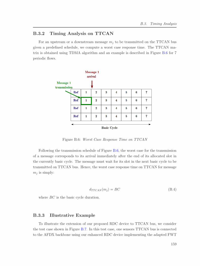
B.3. Timing Analysis
B.3.2 Timing Analysis on TTCAN
For an upstream or a downstream message mj to be transmitted on the TTCAN bus
given a predefined schedule, we compute a worst case response time. The TTCAN ma-
trix is obtained using TDMA algorithm and an example is described in Figure B.6 for 7
periodic flows.
Figure B.6: Worst Case Response Time on TTCAN
Following the transmission schedule of Figure B.6, the worst case for the transmission
of a message corresponds to its arrival immediately after the end of its allocated slot in
the currently basic cycle. The message must wait for its slot in the next basic cycle to be
transmitted on TTCAN bus. Hence, the worst case response time on TTCAN for message
mj is simply:
dTTCAN(mj) = BC (B.4)
where BC is the basic cycle duration.
B.3.3 Illustrative Example
To illustrate the extension of our proposed RDC device to TTCAN bus, we consider
the test case shown in Figure B.7. In this test case, one sensors TTCAN bus is connected
to the AFDX backbone using our enhanced RDC device implementing the adapted FWT
159

Appendix B. Generalization for TTCAN bus
Figure B.7: TTCAN bus interconnected to the AFDX
and MSP strategies. The TTCAN supports upstream flows reported in Table B.1. Espe-
cially, we focus on the impact of frame packing on the AFDX bandwidth consumption.
Table B.1: Upstream flows description
Messages Number Payload(bytes) Period(ms)
m1 3 8 4
m2 2 8 8
m3 16 2 16
m4 4 2 32
The considered TTCAN schedule to transmit these upstream flows is shown in Figure
B.8. The basic cycle is considered equal to T1/2 = 2ms. For space limitation reasons,
we reported the consecutive slots assigned for messages from the same type as one slot
denoted by nj × mj , where nj is the number of messages from type mj . For example, cell
3 × m1 in the schedule of Figure B.8 corresponds to three consecutive slots supporting
messages of type m1.
160

B.3. Timing Analysis
Figure B.8: TTCAN schedule example for TTCAN upstream flows
Table B.2: VLs characteristics under FWT for TTCAN
FWT configuration BAG (ms) MFS (bytes) VLs number rate (Mbps)
∆1 = 0.5ms 2 99 5 1.98
∆1 = 1ms 2 117 3 1.4
Table B.3: End-to-end delay bounds under FWT strategy with ∆ = 1ms
Message type T (ms) deed(ms)
m1 4 3.95
m2 8 4.1
m3 16 4.3
m4 32 4.7
The allocated VLs for upstream flows under FWT strategies with ∆ equal to 0.5ms
and 1ms are reported in Table B.2. For instance, implementing FWT strategy with
∆ = 1ms requires 3 VLs with a BAG of 2 ms and a MFS of 117 bytes. The end-to-end
delay bound is computed for each message under each of the considered FWT configu-
rations and is then compared to its respective deadline. For instance, in Table B.3, the
end-to-end delay bounds for upstream flows of Table B.1 under FWT strategy in the
RDC device with waiting time ∆ = 1ms are reported. As we can see, the RDC device
configuration is schedulable, when considering the deadline of each message equal to its
period. The technological latency of the RDC device is assumed ǫ = 0.05ms.
161

Appendix B. Generalization for TTCAN bus
Table B.4: MSP configurations
VL allocation Waiting Timers (Wj)
conf1 v1 : {3 ∗m1}, v2 : {2 ∗m2}, v3 : {16 ∗m3}, v4 : {4 ∗m4} W1 = 0.42ms, W2 = 0.14ms, W3 = 1.2ms, W4 = 0.24ms
conf2 v1 : {3 ∗m1, 2 ∗m2}, v2 : {16 ∗m3, 4 ∗m4} W1 = 0.7ms, W2 = 1.55ms
Then, we consider two MSP packing configurations in the RDC device as shown in
Table B.4. Configuration conf1 corresponds to packing all the messages of type mi within
the same AFDX frame supported by the virtual link vi. Whereas, configuration conf2
consists in packing messages from types m1 and m2 in virtual link v1, and packing mes-
sages from types m3 and m4 in virtual link v2. The waiting timers used to perform the
frame packing process for each configuration are also provided. For instance, to set up
conf2 in the RDC device, we have W1 = 0.7ms for v1 and W2 = 1.55 for v2.
Table B.5: TTCAN-AFDX RDC: schedulability test and AFDX bandwidth consumption
Configuration Number of VLs AFDX Bandwidth (in Mbps) Schedulability
(1:1) 25 1.42 OK
FWT (∆ = 1ms) 3 1.4 OK
MSP (conf1) 4 1.39 OK
MSP (conf2) 2 0.85 OK
As we can notice from Table B.5, although the FWT strategy with ∆ = 1ms reduces
the number of allocated VLs for the RDC device on AFDX, the induced bandwidth con-
sumption is similar to (1:1) strategy. The MSP strategy offers the best resource utilization
performance, with reference to (1:1) and FWT strategies. For instance, using the adapted
MSP strategy for TTCAN under conf2 reduces the AFDX bandwidth consumption where
a reduction of 40% is noticed with reference to the (1:1) and FWT strategies. Hence, the
FWT does not offer AFDX bandwidth enhancements when used in the RDC device with
TTCAN, whereas, MSP offers an improvement compared to the (1:1) strategy. This is
mainly due to the fact that TTCAN is based on a static schedule for data transmission
and it is more convenient to use MSP which is a static packing strategy. The MSP per-
forms a more accurate VLs allocation and overcomes the over-dimensioning problem of
the FWT strategy.
162

Bibliography
[1] Airlines Electronic Engineering Committee. Aircraft Data Network Part 7, AFDX
network, Arinc Specification 664. Annapolis, Maryland, 2002. Aeronautical Radio.
[2] Avionic Systems Standardisation Committee. Guide to avionics data buses, ARINC
429. 1995.
[3] Robert Bosch GmbH. CAN specification Version 2.0. 1991.
[4] Airlines Electronic Engineering Committee. ARINC Report 655: Remote Data Con-
centrator(RDC) generic description. Annapolis, Maryland, 1999. Aeronautical Radio.
[5] Avionic Systems Standardisation Committee. Avionics Application Software Stan-
dard Interface Part 1-2, ARINC Specification 653P1-2. 2005.
[6] A. Mifdaoui and H. Ayed. WOPANets: a tool for WOrst case Performance Analysis
of embedded Networks. CAMAD 2010.
[7] C. Watkins and R. Walter. Transitioning From Federated Avionics Architectures To
integrated Modular Avionics. Digital Avionics Systems Conference (DASC), 2007.
[8] Condor Engineering Incorporated. MIL-STD-1553 Designer guide.
http://www.condoreng.com/support/downloads/tutorials/MIL-STD-1553Tutorial,
1982.
[9] Avionic Systems Standardisation Committee. ARINC 629 P1-4 Multi-Transmitter
Data Bus, Part1, Technical Description. 1995.
[10] P. Bieber, F. Boniol, M. Boyer, E. Noulard, and C. Pagetti. New Challenges for
Future Avionic Architectures. Aerospacelab, Issue 4, May 2012.
[11] R.I. Davis, A. Burns, R.J. Bril, and J.J. Lukkien. CAN schedulability analysis:
Refuted, revisited and revised. Real-Time Systems, 35(3):239–272, 2007.
[12] A. Al Sheikh, O. Brun, M. Cheramy, and P.E. Hladik. Optimal Design of Virtual
Links in AFDX Networks. Real-Time Systems, May 2013.
[13] A. Al Sheikh, O. Brun, and P.E. Hladik. Partition Scheduling on an IMA Platform
with Strict Periodicity and Communication Delays. In 18th International Conference
on Real-Time and Network Systems, November 2010.
163

Bibliography
[14] R. Saket and N. Navet. Frame packing algorithms for automotive applications. Jour-
nal of Embedded Computing, 2:93–102, 2006.
[15] S.M. Ricardo, N. Navet, and F. Simonot-Lion. Frame Packing under real-time con-
straints. 5th IFAC, 2003.
[16] P. Pop, P. Eles, and Z. Peng. Schedulability-driven frame packing for multicluster
distributed embedded systems. ACM Transactions on Embedded Computing Systems
(TECS), February 2005.
[17] J. Grieu. Analyse et valuation de techniques de commutation Ethernet pour
l’interconnexion de systemes avioniques. PhD thesis, INP, Toulouse, 2004.
[18] Henri Bauer, Jean-Luc Scharbarg, and Christian Fraboul. Improving the worst-case
delay analysis of an AFDX network using an optimized trajectory approach. IEEE
Transactions on Industrial Informatics, 2010.
[19] E. Clarke, O. G. Jr., and D. A. Peled. Model Checking. MIT Press, Cambridge, MA,
USA, 2000.
[20] J.Y. Leboudec and P. Thiran. Network Calculus. Springer Verlag LNCS volume 2050,
2001.
[21] F. Frances, C. Fraboul, and J. Grieu. Using Network Calculus to optimize the AFDX
Network. Proceedings of the 3rd European Congress Embedded Real Time Software,
2006.
[22] S. Martin. Maıtrise de la dimension temporelle de la qualite de service dans les
reseaux. PhD thesis, Universite Paris XII, 2004.
[23] J. Migge. L’ordonnancement sous contraintes temps-reel : un modele a base de
trajectoires. PhD thesis, INRIA, Sophia Antipolis, 1999.
[24] H. Charara, J.L Scharbarg, J. Ermont, and C. Fraboul. Methods for bounding end-to
end delays on an AFDX network. Proceedings of the 18th Euromicro Conference o
n Real-Time Systems, 2006.
[25] K.W. Tindell, A. Burns, and A. J. Wellings. Calculating Controller Area Network
(CAN) message response times. Control Engineering Practice, 3, August 1995.
[26] R.I. Davis, S. Kollmann, V. Pollex, and F. Slomka. Controller Area Network (CAN)
Schedulability Analysis with FIFO Queues. 23rd Euromicro Conference on Real-Time
Systems, 2011.
[27] R.I. Davis, N. Navet, D. Bertrand, and P.M. Yomsi. Controller Area Network (CAN):
Response Time Analysis with Offsets. Real-Time Systems, 35(3):239–272, 2007.
[28] J.L. Scharbarg, M. Boyer, and C. Fraboul. CAN-Ethernet architectures for real-time
applications. IEEE ETFA, 2005.
164

[29] B. Somers. Investigation of a Flexray - CAN Gateway in the Implementation of
Vehicle Speed Control. PhD thesis, Waterford Istitute of Technology, Ireland, 2009.
[30] Stock Flight Systems. CANAerospace: Interface specification for airborne CAN ap-
plications V 1.7. 2006.
[31] Airlines Electronic Engineering Committee. ARINC Specification 825-2: General
standardization of CAN (Controller Area Network) bus protocol for airborne use.
Annapolis, Maryland, 2011. Aeronautical Radio.
[32] S. Zeng and N. Uzun. A hierarchical traffic shaper for packet switches. Global
Telecommunications Conference, GLOBECOM, 1999.
[33] J. S. Turner. New Directions in Communications (or Which Way to the Information
Age?). IEEE Communications Magazine, 1986.
[34] J.L. Valenzuela, A. Monleon, I. San Esteban, M. Portoles, and O. Sallent. A hierarchi-
cal token bucket algorithm to enhance qos in ieee 802.11: proposal, implementation
and evaluation. In Vehicular Technology Conference, 2004.
[35] T. Nolte, M. Sjodin, and H. Hansson. Server-based scheduling of the CAN bus.
Emerging Technologies and Factory Automation (ETFA), 2003.
[36] Z. Iqbal, L. Almeida, R. Marau, M. Behnam, and T. Nolte. Implementing hierarchical
scheduling on cots ethernet switches using a master/slave approach. In 7th IEEE
International Symposium on Industrial Embedded Systems, 2012.
[37] E. Wandeler, A. Maxiaguine, and L. Thiele. On the Use of Greedy Shapers in Real-
Time Embedded Systems. Embedded Computing Systems, 2012.
[38] R.I. Davis and N. Navet. Traffic Shaping to Reduce Jitter in Controller Area Network
(CAN). 24th Euromicro Conference on Real-Time Systems, 2012.
[39] P. Narasimhan, L. Moser, and P. Melliar-Smith. Message packing as a performance
enhancement strategy with application to the totem protocols. In Global Telecom-
munications Conference (GLOBECOM), 1996.
[40] R. Marau, N. Figueiredo, R. Santos, P. Pedreiras, L. Almeida, and T. Nolte. Towards
Server-based Switched Ethernet for real-time communications. Proceedings of the
1st Workshop on Compositional Theory and Technology for Real-Time Embedded
Systems, 2008.
[41] E. G. Coffman, M. R. Garey, and D. S. Johnson. Approximation algorithms for
NP-hard problems. PWS Publishing Company, 1996.
[42] E. L. Lawler and D. E. Wood. Branch-and-bound methods: A survey. Operations
Research, 1966.
165

Bibliography
[43] A. Albert, R. Strasser, and A. Trachtler. Migration from CAN to TTCAN for a
Distributed Control System. ICC, 2003.
[44] Xin Qiao, Kun-FengWang, Yuan Sun, Wu-Ling Huang, and Fei-YueWang. A Genetic
Algorithms based optimization for TTCAN. In IEEE International Conference on
Vehicular Electronics and Safety, 2007.
[45] A. Hara, K. Fonseca, and L. Scandelari. CAN/TTCAN Simulator System based on
Educational DSP Hardware Kits. ICC, 2003.
166