doctor of philosophy - opus at uts: home · pdf filein this thesis, a series of laboratory...

Analysing Consolidation Data to Optimise Elastic Visco–

plastic Model Parameters for Soft Clay

A thesis in fulfilment of the requirement for the award of the degree

Doctor of Philosophy

from

University of Technology, Sydney (UTS)

By

THU MINH LE, BEng (1st class Hons, UTS)

School of Civil and Environmental Engineering, Faculty of Engineering and Information Technology

2015

ii

CERTIFICATE OF ORIGINAL AUTHORSHIP

I certify that the work in this thesis has not previously been submitted for a degree nor has it been submitted as part of requirements for a degree except as fully acknowledged within the text.

I also certify that the thesis has been written by me. Any help that I have received in my research work and the preparation of the thesis itself has been acknowledged. In addition, I certify that all information sources and literature used are indicated in the thesis.

Thu Minh Le

Feburary 2015

iii

ABSTRACTAnalysing the behaviour of soft soils under embankments is a significant challenging

task for geotechnical engineers. By having more insight into long term soil behaviour

and understanding the key parameters influencing the results, there will be more chance

to strategically plan and utilise the soft ground for construction purposes. The time–

dependent behaviour of soft soils, especially the ground settlements under structural and

non–structural loading, is considered as a significant issue, which has been studied for

many decades. Prediction of creep settlement of soft soils is a challenging task, as a

very long period of time counted in years is involved. Many theories have been

proposed along with a large number of laboratory and field measurements in order to

provide more precise knowledge of the time–dependent viscous behaviour of soft soils.

However, there are still some disagreements between theoretical and practical studies,

which may keep the accuracy of the predictions questionable.

Among the great number of developed models for soft soils, the elastic visco–

plastic model with the non–linear creep function is considered as an effective method to

describe the long–term stress–strain behaviour of soft soils. However, the difficulties to

determine the model parameters limit the application of the model in practice. Since the

relationship between the effective stress and strain during the dissipation of the excess

pore water pressure cannot be identified easily, in the current practice the creep strain

limit and the creep coefficient to form the creep function are determined

based on the curve fitting of the experimental data after the end of the primary

consolidation. As a result, the number of data points available for the curve fitting is

limited, and the extremely long tests are required. Moreover, in the conventional

procedure for the ease of the curve fitting, the time parameter to in the elastic visco–

plastic, which is the time value of the reference time line in the space of -log( ’z), has

been assumed as the time at the end of primary consolidation process. Hence, based on

this assumption of to, the reference time line would include viscous strain, which is

contradict to the definition of a viscous free reference time line. Thus, the value of to

influences not only the reference time line parameters, but also the parameters of the

creep function. Additionally, the conventional determination approach for the model

parameters is influenced by the thickness of the soil sample. Hence, the model

parameters obtained by the conventional method may not be unique.

iv

As a result, the main objective of this research project is to propose a numerical

solution to determine the model parameters for the elastic visco–plastic model adopting

the trust–region reflective least square algorithm. The trust-region reflective least square

algorithm is an advanced optimisation method for the non-linear equation system. A

Crank–Nicolson finite difference scheme is applied to solve the coupled partial

differential equations in order to simulate one-dimensional stress-strain behaviour of

soft soil with different boundary conditions. The proposed method can adopt the

experimental data during the dissipation of the excess pore water pressure to determine

all the model parameters simultaneously.

In this thesis, a series of laboratory experiments were conducted at the UTS soil

laboratory using two sizes of hydraulic consolidation Rowe cell setups. A 29.5 mm

thick soil sample of a kaolinite mixture was tested and adopted to determine the model

parameters, while an experimental result of a thicker soil sample (i.e. 140.5 mm thick)

was compared with the predictions using the optimised model parameters. The Rowe

cell setups can measure the volume change, the vertical settlement and the excess pore

water pressure continuously. Especially, the large Rowe cell setup to conduct the test on

the 140.5 mm thick soil sample was modified to measure the excess pore water pressure

at different depth and different distances to the centre line at the base. Moreover, other

four validation exercises including two laboratory–based case studies and two field–

based case studies were included to verify the ability of the proposed method to analyse

the time-dependent behaviour of soft soils.

The developed method can be considered as a simple, practical and accurate

solution for the model parameter determination. The optimised model parameters allow

the predictions of settlement to be in good agreement with the measurements, while the

predictions of the excess pore water pressure are reasonably close to the measurement.

Additionally, the variations of the creep strain limit, the creep coefficient and the creep

strain rate during the dissipation of the excess pore water pressure can be observed.

Moreover, the unusual increase of the excess pore water pressure in the early stages of

loading can be also predicted. The numerical analysis applying the proposed method is

able to illustrate the influence of the soil layer thickness on the time–dependent stress-

strain behaviour of soft soil. The proposed approach can be adopted to back calculate

the elastic visco-plastic model parameters for real case in the field utilising time-

dependent settlement and excess pore water pressure measurements.

v

To my father, Pha Van Le, my mother, The Thanh T. Truong, my brother, Tri

Minh Le and my husband, Thanh Tien Nguyen, whose love, encouragement and

support have been always with me through this journey.

vi

ACKNOWLEDGEMENT I have discovered that researching and writing this thesis is both challenging and

pleasant experience in my life. My PhD journey would not have been completed without

accompany and supports from various groups of staff and friends. It is my pleasure to

express my gratitude for all of them.

Firstly, I would like to express my greatest appreciation to my principal supervisor,

Dr. Behzad Fatahi, and my co-supervisor, A/Prof. Hadi Khabbaz, who provide me this

opportunity, encourage, assist and support me through my study. Their guidance, their time,

ideas and support have inspired and motivated me in many aspects of my PhD study as well

as my life.

I would like to thank Antonio Reyno, and other staff members in the university laboratories

for their assistances and supports in my laboratory experiments. I am grateful to Babak

Azari, Lam Nguyen and Liem Ho which have helped me to prepare and operate the

equipments for my laboratory tests. I also appreciate the general assistance from Phyllis

Agius and Van Le during my study.

The research effort in this thesis was carried out during 2010-2014 in the Faculty of

Engineering and Information Technology of University of Technology, Sydney. It has been

supported by the Australian Postgraduate Awards from the Australian Government in three

and a half years. The financial supports from the university and the faculty during my study

are gratefully acknowledged.

Thanks are extended to my friends and fellow friends at University of Technology,

Sydney, whose accompany and helps have made my study life more enjoyable. For my

geotechnical group members, particularly Babak Arazi, Behnam Fatahi, Ali Parsa-Pajouh,

Lam Nguyen, Aslan Sadeghi Hokmabadi, Liem Ho, and Quoc Van Nguyen.

Lastly, I would like to express my love and appreciation to my family for their love,

encouragement and support. My parents endlessly love me and always encourage me to

study and follow my pursuits. My parents are not only my family, but also my lifetime

teachers and my idols. I am also grateful to my brother for his presence at Sydney to bring

me sense of family, while my parents are still in Vietnam. Additionally, I am indebted to

my grandmother, my aunty and her family here for their caring and essential supports from

the first day of my arrival in Sydney and now. And for my loving, supportive and patient

husband Thanh, I appreciate his love and faithful support during the final stages of my PhD

study.

vii

LIST OF PUBLICATIONS Published/Accepted Journal Papers

Fatahi, B., Le, T.M., & Khabbaz, H. 2012, Effects of Initial Stress State on

Performance of Embankments on Soft Soils. Australian Geomechanics Journal,

47(3), 77-88.

Le, T.M., Fatahi, B. & Khabbaz, H. 2012, 'Viscous Behaviour of Soft Clay and

Inducing Factors', Geotechnical and Geological Engineering: an international

journal, 30(5), pp. 1069-1083

Fatahi, B., Le, T.M., Fatahi, B., & Khabbaz, H. 2013, Shrinkage Properties of Soft Clay

Treated with Cement and Geofibers. Geotechnical and Geological

Engineering, 31(5), 1421-1435.

Fatahi, B., Fatahi, B., Le, T.M., & Khabbaz, H. 2013, Small-strain Properties of Soft

Clay Treated with Fibre and Cement. Geosynthetics International, 20(4), 286-300.

Fatahi, B., Le, T.M., Le, M. Q., & Khabbaz, H. 2013, Soil Creep Effects on Ground

Lateral Deformation and Pore Water Pressure under Embankments.

Geomechanics and Geoengineering, 8(2), 107-124.

Le, T.M., Fatahi, B., & Khabbaz, H. 2015, Numerical Optimisation to Obtain Elastic

Viscoplastic Model Parameters for Soft Clay. International Journal of

Plasticity, 65, 1-21.

Le, T.M., Fatahi, B., Disfani, M., & Khabbaz, H. 2015, Analysing Consolidation Data

to Obtain Elastic Viscoplastic Parameters of Clay. Geomechanics and

Engineering: an International Journal, 8(4).

Submitted Journal Papers

Trust-region Reflective Optimisation to Obtain Soil Visco-plastic Properties,

Engineering Computations

Numerical Optimisation Using Trust-region Reflective Least Squares Algorithm to

Obtain Non-linear Creep Parameters of Soil, Applied Mathematical Modelling

Conference Papers

viii

Le, T.M., Fatahi, B., & Khabbaz, H. 2011, Soil Creep Mechanisms and Inducing

Factors, Proceedings of International Conference on Advances in Geotechnical

Engineering, Curtin University, Perth, Australia, 241-248.

Fatahi, B., Khabbaz, H., & Le, T.M. 2012, Improvement of Rail Track Subgrade Using

Stone Columns Combined with Geosynthetics, Proceedings of the 2nd Advanced

in Transportation Geotechnics, Taylor & Francis Group, Sapporo, Japan, 202-206

Le, T.M., Le, P.V., Khabbaz, H., & Fatahi, B. 2013, Stability and Deformation of Sheet

Pile Walls for Protecting Riverside Structures in the Mekong River Delta.

Proceedings of Geo-Congress: Stability and Performance of Slopes and

Embankments III, ASCE, San Diego, USA, 1349-1358

Fatahi, B., Le, T.M., & Khabbaz, H. 2013, Influence Of Insitu Stresses on Deformation

and Stability of Embankments on Deep Clays, Proceedings of the International

Conference on Ground Improvement and Ground Control: Transport

Infrastructure Development and Natural Hazards Mitigation, Research

Publishing, Wollongong, Australia, 491-496

Fatahi, B., Le, T.M., & Khabbaz, H. 2013, Influence of Soil Creep on Stability of

Embankment on Soft Soil, Proceedings of the International Conference on

Ground Improvement and Ground Control: Transport Infrastructure

Development and Natural Hazards Mitigation, Research Publishing, Wollongong,

Australia, 485-490

Le, T.M., Fatahi, B., & Khabbaz, H. 2014, Numerical Solution to Predict Visco-Plastic

Model Parameters of Soft Clay during Excess Pore Water Pressure Dissipation,

Proceedings of the 8th European Conference on Numerical Methods in

Geotechnical Engineering, Taylor & Francis Group, Delft, the Netherlands, 175-

180

ix

TABLE OF CONTENTS

ABSTRACT ............................................................................................................................... III

ACKNOWLEDGEMENT ........................................................................................................ VI

LIST OF PUBLICATIONS ................................................................................................... VII

TABLE OF CONTENTS ......................................................................................................... IX

LIST OF TABLES ................................................................................................................. XIII

LIST OF FIGURES ................................................................................................................. XV

LIST OF NOTATIONS ........................................................................................................ XXV

CHAPTER 1

1 INTRODUCTION ........................................................................................................... 1-1

1.1 OVERVIEW ................................................................................................................ 1-1

1.2 STATEMENT OF PROBLEM ......................................................................................... 1-3

1.3 OBJECTIVES AND SCOPES OF RESEARCH ................................................................... 1-6

1.4 ORGANISATION OF THE THESIS ................................................................................. 1-7

CHAPTER 2

2 LITERATURE REVIEW ............................................................................................... 2-1

2.1 INTRODUCTION ......................................................................................................... 2-1

2.2 PROBLEMS ASSOCIATED WITH SOFT SOILS ............................................................... 2-2

2.2.1 Description of soft soils ........................................................................................ 2-2

2.2.2 Problems associated with soft soils ...................................................................... 2-6

2.3 CREEP MECHANISMS ................................................................................................. 2-7

2.3.1 Creep due to the breakdown of inter–particle bonds ........................................... 2-7

2.3.2 Creep due to jumping of molecule bonds ............................................................. 2-9

2.3.3 Creep due to sliding among particles ................................................................ 2-11

2.3.4 Creep due to water flows in a double pore system ............................................. 2-12

2.3.5 Creep due to the structural viscosity .................................................................. 2-14

2.3.6 Discussion .......................................................................................................... 2-17

2.4 TIME–DEPENDENT STRESS – STRAIN BEHAVIOUR OF SOFT SOILS ........................... 2-20

2.4.1 Time effects ......................................................................................................... 2-20

2.4.2 Strain rate effects ............................................................................................... 2-23

x

2.4.3 Stress effects ........................................................................................................ 2-27

2.4.4 Other influencing factors .................................................................................... 2-29

2.4.5 Stress relaxation ................................................................................................. 2-31

2.4.6 Undrained creep ................................................................................................. 2-31

2.5 HYPOTHESES A AND B ............................................................................................ 2-33

2.5.1 The suppositions ................................................................................................. 2-35

2.5.2 Discussion on the uniqueness concept of the end of primary consolidation void

ratio 2-38

2.5.3 Laboratory study on soil samples with different thicknesses .............................. 2-40

2.6 PREDICTION APPROACHES FOR THE LONG-TERM SETTLEMENT OF SOFT SOILS ....... 2-45

2.6.1 Approach of coupling the consolidation theory and a constant C .................... 2-45

2.6.2 The concept of unique C /Cc and eEOP ................................................................ 2-49

2.6.3 General stress – strain – strain rate models ....................................................... 2-49 2.6.3.1 Isotach models ................................................................................................................... 2-49 2.6.3.2 Time resistance concept ................................................................................................... 2-55 2.6.3.3 Other models ..................................................................................................................... 2-58

2.7 SUMMARY ............................................................................................................... 2-61

CHAPTER 3

3 NUMERICAL SOLUTION FOR ELASTIC VISCO–PLASTIC MODEL AND

MODEL PARAMETER DETERMINATION ...................................................................... 3-1

3.1 INTRODUCTION .......................................................................................................... 3-1

3.2 ELASTIC VISCO–PLASTIC MODEL............................................................................... 3-1

3.2.1 Time–line concept ................................................................................................. 3-1

3.2.2 Governing equations ............................................................................................. 3-6

3.2.3 Conventional procedure for the model parameter determination ........................ 3-8 3.2.3.1 Instant time-line parameters ( /V and ) ...................................................................... 3-9 3.2.3.2 Creep function parameters ( /V, and to) ............................................................... 3-10 3.2.3.3 Reference time-line parameters ( /V, and ’zo) ..................................................... 3-17 3.2.3.4 Numerical analysis for an example embankment on Ottawa clay ............................. 3-21

3.3 COUPLED EQUATIONS OF THE EVP MODEL AND THE CONSOLIDATION THEORY .... 3-27

3.3.1 Coupled governing equations for a constant external loading ........................... 3-27

3.3.2 Crank-Nicolson finite difference solution ........................................................... 3-29

3.3.3 Time-dependent loading ..................................................................................... 3-36

3.4 MODEL PARAMETER DETERMINATION .................................................................... 3-37

3.4.1 General ............................................................................................................... 3-37

3.4.2 Least squares algorithm ..................................................................................... 3-37

xi

3.4.3 Trust–region reflective algorithm ...................................................................... 3-38

3.4.4 Parameters determination solution .................................................................... 3-41

3.5 SUMMARY ............................................................................................................... 3-45

CHAPTER 4

4 LABORATORY STUDY TO VERIFY THE PROPOSED NUMERICAL

APPROACH ............................................................................................................................. 4-1

4.1 GENERAL .................................................................................................................. 4-1

4.2 SMALL ROWE CELL EXPERIMENT AND PARAMETER DETERMINATION ..................... 4-1

4.2.1 Test setup and experimental procedure ............................................................... 4-2 4.2.1.1 Soil sample preparation ..................................................................................................... 4-2 4.2.1.2 Experiment on thin KBS sample ....................................................................................... 4-4 4.2.1.3 EVP model parameter determination ............................................................................ 4-10

4.3 LARGE ROWE CELL EXPERIMENT AND VERIFICATION EXERCISE ........................... 4-16

4.3.1 Experimental setup and testing procedure ......................................................... 4-16

4.3.2 Experimental results and verification exercise .................................................. 4-21

4.4 DISCUSSION ............................................................................................................ 4-26

4.5 SUMMARY ............................................................................................................... 4-34

CHAPTER 5

5 LABORATORY-BASED CASE STUDIES FOR FURTHER VALIDATION ......... 5-1

5.1 GENERAL .................................................................................................................. 5-1

5.2 CASE STUDY 1: HONG KONG MARINE CLAY, HONG KONG ...................................... 5-2

5.2.1 Soil properties ...................................................................................................... 5-2

5.2.2 Numerical simulation ........................................................................................... 5-2

5.2.3 Results and discussion .......................................................................................... 5-8

5.3 CASE STUDY 2: DRAMMEN CLAY, NORWAY ........................................................... 5-25

5.3.1 Soil properties .................................................................................................... 5-25

5.3.2 Numerical simulation ......................................................................................... 5-26

5.3.3 Results and discussions ...................................................................................... 5-29

5.4 SUMMARY ............................................................................................................... 5-50

CHAPTER 6

6 FURTHER VERIFICATION EXERCISES–FIELD CASE STUDIES ..................... 6-1

6.1 INTRODUCTION ......................................................................................................... 6-1

6.2 CASE STUDY 1: VÄSBY TEST FILL ............................................................................. 6-1

6.2.1 Project and site description.................................................................................. 6-1

xii

6.2.2 Subsoil profile and soil properties ........................................................................ 6-4

6.2.3 Numerical simulation and analysis ....................................................................... 6-5 6.2.3.1 Model parameter determination ....................................................................................... 6-5 6.2.3.2 Numerical modelling of Väsby test fill .......................................................................... 6-13

6.2.4 Results and discussion ........................................................................................ 6-20 6.2.4.1 Settlement predictions ...................................................................................................... 6-20 6.2.4.2 Excess pore water pressure ............................................................................................. 6-23 6.2.4.3 Creep compression properties ........................................................................................ 6-26

6.3 CASE STUDY 2: SKÅ-EDEBY TEST FILL ................................................................... 6-34

6.3.1 Project and site description ................................................................................ 6-34

6.3.2 Subsoil profile and soil properties ...................................................................... 6-37

6.3.3 Numerical simulation .......................................................................................... 6-39 6.3.3.1 Model parameter determination ..................................................................................... 6-39 6.3.3.2 Numerical modelling for Skå Edeby test fill ................................................................. 6-52

6.3.4 Results and discussion ........................................................................................ 6-58 6.3.4.1 Settlement predictions ...................................................................................................... 6-58 6.3.4.2 Excess pore water pressure ............................................................................................. 6-62 6.3.4.3 Creep compression properties ........................................................................................ 6-66

6.4 SUMMARY ............................................................................................................... 6-73

CHAPTER 7

7 CONCLUSIONS AND RECOMMENDATIONS ......................................................... 7-1

7.1 SUMMARY ................................................................................................................. 7-1

7.2 CONCLUSIONS ........................................................................................................... 7-3

7.3 RECOMMENDATIONS FOR FUTURE RESEARCH .......................................................... 7-7

REFERENCES ..................................................................................................................... Ref-1

xiii

LIST OF TABLES Table 2.1 Flocculation and dispersion of Clays (after Mitchell 1956) .......................... 2-4

Table 2.2 Consistency of fine grained soils by consistency index and undrained shear

strength ............................................................................................................. 2-5

Table 2.3 Types of peds and pores (after Matsuo & Kamon 1977) ............................ 2-13

Table 2.4 Main creep mechanisms in soft soils ........................................................... 2-18

Table 2.5 Secondary compression based on C .......................................................... 2-48

Table 2.6 Summary of existing model category (modified after Leroueil 1985) ........ 2-61

Table 2.7 Comparison of some constitutive models for time-dependent behaviour of soft

soils ................................................................................................................ 2-63

Table 3.1 Influences of to on o/V and of Ottawa clay ......................................... 3-11

Table 3.2 Options to determine the reference time-line parameters ............................ 3-23

Table 3.3 The EVP model parameters by different options ......................................... 3-23

Table 4.1 Properties of Q38 kaolinite and Active Bond 23 bentonite ........................... 4-2

Table 4.2 Initial information adopted in the optimisation procedure to determine the

model parameters for KBS mixture ............................................................... 4-11

Table 4.3 The optimised model parameters and soil permeability properties ............. 4-12

Table 4.4 Details of loading stages using LRC apparatus ........................................... 4-20

Table 4.5 Initial input information for LRC simulation ............................................... 4-20

Table 5.1 Initial information adopted in the optimisation procedure to determine the

model parameters for Hong Kong marine clay ................................................ 5-3

Table 5.2 Summary of the adopted model parameters for Hong Kong marine clay ..... 5-6

Table 5.3 Initial information of four specimens of Drammen clay (after Berre & Iversen

1972) .............................................................................................................. 5-27

Table 5.4 Model parameters for Drammen clay obtained adopting the proposed TRRLS

approach ......................................................................................................... 5-29

Table 6.1 Initial information adopted for the EVP model parameter determination for

Väsby clay ........................................................................................................ 6-9

Table 6.2 The optimised model parameters and soil permeability properties for Väsby

clay ................................................................................................................. 6-12

xiv

Table 6.3 Initial values of mv and cv reported by Chang (1969) and calculated coefficient

of permeability k based on mv and cv ............................................................ 6-14

Table 6.4 Soil properties of Samples A and B of Skå-Edeby clay .............................. 6-43


Skå-Edeby Sample A of Skå-Edeby clay ...................................................... 6-44

Table 6.6 The optimised model parameters and soil permeability properties of Sample A

of Skå-Edeby clay .......................................................................................... 6-45


Sample B of Skå-Edeby clay ......................................................................... 6-49

Table 6.8 The optimised model parameters and soil permeability properties of for

Sample B of Skå-Edeby clay ......................................................................... 6-49

xv

LIST OF FIGURES Figure 1.1 Port of Brisbane Expansion project

(http://www.portstrategy.com/__data/assets/image/0003/531534/Port-of-

Brisbane-aerial-2010.jpg) ................................................................................ 1-2

Figure 1.2 Port of Botany Bay Extension

(http://www.infrastructure.org.au/Content/2012NationalInfrastructureAwards.a

spx) ................................................................................................................... 1-3

Figure 1.3 Typical settlement curve ............................................................................... 1-4

Figure 2.1 (a) Water molecule and (b) Attraction of water molecules on the surface of

clay particle (modified after Ranjan & Rao 2007) ........................................... 2-3

Figure 2.2 A schematic view of a soil element of soil in macroscopic scale ................. 2-8

Figure 2.3 Schematic representation of an ion surrounded by water molecules, and the

energy barrier which it must surmount in moving between equilibrium

positions (after Low 1962) ............................................................................. 2-10

Figure 2.4 Contact mechanism used for individual particles in numerical model: (a)

Normal force mechanism, and (b) Tangential force mechanism (after Kuhn &

Mitchell 1993) ................................................................................................ 2-12

Figure 2.5 Schematic concept of clay structure (modified afterZeevart 1986) ............ 2-13

Figure 2.6 A schematic view of clay–water system ..................................................... 2-15

Figure 2.7 Schematic clay-water system in (a) free water flows through the pore system

from the beginning of the whole compression process, (b) after free water

flowed out of the pores .................................................................................. 2-20

Figure 2.8 (a-b) Creep stages and strain rates in creep tests performed by triaxial

apparatus and (c-d) Compression stages and strain rates in step load tests by

oedometer apparatus (after Augustesen et al. 2004) ...................................... 2-22

Figure 2.9 Laboratory stress – strain curves of Berthieville test fill samples at different

depths (after Kabbaj et al. 1988) .................................................................... 2-23

Figure 2.10 Constant rate of strain (CRS) tests (a) the variation of strain with time at

different strain rates, and (b) stress – strain relationship at different strain rates

(after Augustesen et al. 2004) ........................................................................ 2-24

Figure 2.11 Constant rate of strain tests on (a) Bastican clay and (b) St. Cesaire clay

(after Lerouiel et al. 1985) ............................................................................. 2-25

xvi

Figure 2.12 EOP e–log ’v curves from CRS and incremental loading (IL) oedometer

tests of Berthierville clay (after Mesri & Feng, 1986) ................................... 2-26

Figure 2.13 Ranges of strain rates in the laboratory tests and in-situ (after Leroueil

2006) .............................................................................................................. 2-27

Figure 2.14 (a) Types of compression curves dependent on the stress level (after

Leroueil et al. 1985) and (b) the corresponding strain rate (after Augustesen et

al. 2004) ......................................................................................................... 2-28

Figure 2.15 Several single loading tests on Batiscan clay indicating the effects of stress

increments on the variation of strain-time behaviour (after Leroueil et al. 1985)

....................................................................................................................... 2-29

Figure 2.16 Stress – strain curves of Berthierville clay at different strain rates and

different temperatures tested by Boudali et al. 1994 (after Leroueil 1996) ... 2-30

Figure 2.17 The variations of the axial strains and excess pore water pressure with time

during undrained triaxial creep tests on (a-b) Ko-consolidated Wenzhou marine

clay and (b-c) isotropically consolidated Wenzhou marine clay (after Wang &

Yin 2012) ....................................................................................................... 2-32

Figure 2.18 Void ratio versus time under the applied stress from 'zi to 'zf ............... 2-35

Figure 2.19 Void ratio versus time of thin and thick samples based on Hypothesis A2-36

Figure 2.20 Void ratio versus time of thin and thick samples based on Hypothesis B 2-37

Figure 2.21 Void ratio versus effective stress at the end of primary consolidation (after

Jamiolkowski et al. 1985) .............................................................................. 2-37

Figure 2.22 Vertical strains of soil samples of different thicknesses (after Aboshi 1995)

....................................................................................................................... 2-41

Figure 2.23 Stress – strain curves obtained in laboratory and observed in situ between

4.25m and 7.29m of Vasby test fill (Leroueil & Kabbaj (1987) ................... 2-44

Figure 2.24 Void ratio-effective stress relationship during the consolidation process

(after Taylor & Merchant, 1940) ................................................................... 2-46

Figure 2.25 Definition of instant compression and delayed compression compared to the

primary and secondary compression (after Bjerrum 1967) (a) the change in

effective stress, and (b) compression versus time .......................................... 2-51

Figure 2.26 Time-line system of Bjerrum (after Bjerrum 1967) ................................. 2-51

xvii

Figure 2.27 Time resistance for a load step in an oedometer test (a) the variation of the

excess pore water pressure or strain with time and (b) the variation of time

resistance R with time (after Janbu 1969) ...................................................... 2-56

Figure 2.28 Idealised stress – strain curve from an oedemeter test with the division of

strain increments into an elastic and creep component. Normal consolidation

(NC) line has time value of 1 day ( c+t’ = 1 day on NC) (after Vermeer &

Neher 1999) ................................................................................................... 2-57

Figure 2.29 Creep behaviour obtained in the time resistance concept (after Vermeer &

Neher 1999) ................................................................................................... 2-57

Figure 3.1 The time-line system proposed by Yin (1990) in (a) natural scale and (b) in

logarithm scale of effective stress (after Yin 1990) ......................................... 3-5

Figure 3.2 Illustration of the reference time-line and the limit time-line ....................... 3-6

Figure 3.3 Compression curves of Ottawa marine clay (after Crawford 1964) (a) vertical

strain versus time and (b) vertical strain versus vertical effective stress ......... 3-8

Figure 3.4 Curve fitting for the instant time-line ........................................................... 3-9

Figure 3.5 Linear curve fitting for the creep function parameters applying for Stages 5-

6-7 for to = 45 min .......................................................................................... 3-12


6-7 for to = 55 min .......................................................................................... 3-12


6-7 for to =40 min ........................................................................................... 3-13

Figure 3.8 Relationship between the effective stress and (a) the creep coefficient o/V

and (b) the creep strain limit for to = 45 min ........................................... 3-14


and (b) the creep strain limit for to = 55 min ........................................... 3-15


and (b) the creep strain limit for to = 40 min .......................................... 3-16

Figure 3.11 Schematic time-line concept for the model parameter determination ...... 3-18

Figure 3.12 Time-line system of Ottawa clay adopting to = 45 min ............................ 3-20



Figure 3.15 Soil profile adopted in the example calculation ....................................... 3-24

xviii

Figure 3.16 Variations of the initial overburden effective stress, final effective stress and

the vertical applied pressure with depth under the example embankment .... 3-25

Figure 3.17 Settlement prediction for Ottawa clay under the embankment adopting three

sets of model parameters in Table 3.3 ........................................................... 3-26

Figure 3.18 Variations of the excess pore water pressure with depth at (a) 25 years and

(b) 50 years after construction of Ottawa clay under the embankment adopting

three sets of model parameters in Table 3.3 .................................................. 3-27

Figure 3.19 Calculation grid and the boundary conditions of the Crank-Nicolson finite

difference solution for the partial differential equations for one way drainage

condition ........................................................................................................ 3-30

Figure 3.20 Calculation grid and the boundary conditions of the Crank-Nicolson finite

difference solution for the partial differential equations for two way drainage

condition ........................................................................................................ 3-30

Figure 3.21 Flowchart for solving the coupled equations of the EVP model and the

consolidation theory ....................................................................................... 3-35

Figure 3.22 Time-dependent loading ........................................................................... 3-36

Figure 3.23 Flowchart of the trust-region reflective method ....................................... 3-40

Figure 3.24 Flowchart for calculating u(x) .................................................................. 3-44

Figure 4.1 KBS mixture (a) dry state of each material and (b) wet mixture ................. 4-3

Figure 4.2 Schematic diagram of the small Rowe cell .................................................. 4-4

Figure 4.3 Small Rowe cell system connection ............................................................. 4-5

Figure 4.4 Small Rowe cell set up in the laboratory ...................................................... 4-6

Figure 4.5 Assembling soil sample in the small Rowe cell (a) soil sample assembled in

the cell and covered by a filter paper, (b) porous plate placed on the soil sample

surface and covered by water, and (c) the soil sample at the end of the test ... 4-7

Figure 4.6 Initial loading stages of Rowe cell consolidation test of 29.5 mm thick KBS

......................................................................................................................... 4-9

Figure 4.7 Unloading stages of Rowe cell consolidation test of 29.5 mm thick KBS ... 4-9

Figure 4.8 Reloading stages of Rowe cell consolidation test of 29.5 mm thick KBS . 4-10

Figure 4.9 Calculation grid for the simulation of SRC sample .................................... 4-12

Figure 4.10 Relation of void ratio and coefficient of permeability ............................. 4-13

Figure 4.11 Predictions and measurements of the SRC sample (a) The average vertical

strain and (b) The excess pore water pressure at the impervious base .......... 4-15

xix

Figure 4.12 Illustration of the large hydraulic consolidation cell (LRC) apparatus .... 4-17

Figure 4.13 Large Rowe cell set up in the laboratory .................................................. 4-17

Figure 4.14 Large Rowe cell system connection ......................................................... 4-18

Figure 4.15 Calculation grid for the numerical simulation of the LRC sample ........... 4-23

Figure 4.16 Prediction of the average vertical strain of the thick sample (LRC) ........ 4-23

Figure 4.17 Excess pore water pressure of LRC during (a) 25 kPa – 50 kPa, and (b) 50

kPa – 100 kPa loading stages ......................................................................... 4-24

Figure 4.18 Excess pore water pressure of LRC during (a) 100 kPa – 200 kPa and (b)

200 kPa – 400 kPa loading stages .................................................................. 4-25

Figure 4.19 Time-line system for the KBS mixture ..................................................... 4-27

Figure 4.20 Variation of the average creep strain limit with time of (a) SRC and (b)

LRC ................................................................................................................ 4-29

Figure 4.21 Variation of the average creep coefficient V with time of (a) SRC and (b)

LRC ................................................................................................................ 4-30

Figure 4.22 Variation of the average creep parameter /V with time of (a) SRC and (b)

LRC ................................................................................................................ 4-32

Figure 4.23 Variation of the average creep strain rate with time of (a) SRC and (b)

LRC ................................................................................................................ 4-33

Figure 4.24 Average vertical strain versus average effective stress ............................ 4-34

Figure 5.1 Experimental loading stages of the Hong Kong marine clay (after Yin 1999)

(a) loading stages, (b) unloading and (c) reloading ......................................... 5-4

Figure 5.2 Relationship between the void ratio and coefficient of permeability

calculated based on cv and mv of the consolidation results from Yin (1999) ... 5-5

Figure 5.3 Predicted time dependent vertical strain under (a) 100 kPa and 200 kPa, (b)

400 kPa and 800 kPa vertical stresses using the parameters by the conventional

method and the optimised parameters using the proposed approach ............... 5-7

Figure 5.4 Predictions of (a) the average strain of various thickness soil layers and (b)

the excess pore water pressure at the base of soil layers adopting model

parameters obtained from the proposed approach and the conventional

approach ......................................................................................................... 5-12

Figure 5.5 Influence of soil thickness on the average vertical strain at 90%, 95% and

98% dissipation of excess pore water pressure at the impervious boundary . 5-13

xx

Figure 5.6 Average creep coefficient ( o/V) predicted by (a) the proposed approach and

(b) the conventional approach ........................................................................ 5-14

Figure 5.7 Average creep strain limit ( ) predicted by (a) the proposed approach and


Figure 5.8 Average creep parameter ( ) predicted by (a) the proposed approach and


Figure 5.9 Average creep strain rate ( ) predicted by (a) the proposed approach and


Figure 5.10 Vertical stress – strain relationship predicted by (a) the proposed approach

and (b) the conventional approach ................................................................. 5-20

Figure 5.11 Isochrones of the variation of the normalised excess pore water pressure

with depth after (a) 1 min, and (b) 1 hour ...................................................... 5-22


with depth after (a) 1 day, and (b) 1 year ....................................................... 5-23


with depth after (a) 2 years, and (b) 10 years ................................................ 5-24

Figure 5.14 Stress – strain curves of oedometer soil sample of different heights (after

Berre & Iversen 1972) ................................................................................... 5-26

Figure 5.15 Void ratio – permeability relationship for Drammen clay ....................... 5-28

Figure 5.16 Comparison of the prediction and the measured data for Test A (0.0188 m):

(a) the average vertical strain, and (b) the excess pore water pressure at the

base for Drammen clay .................................................................................. 5-30

Figure 5.17 Comparison of the prediction and the measured data for Test B (0.075 m):

(a) the average vertical strain and (b) the excess pore water pressure at the base

for Drammen clay .......................................................................................... 5-33

Figure 5.18 Comparison of the prediction and the measured data for Test C (0.150 m):

(a) the average vertical strain and (b) the excess pore water pressure at the base

for Drammen clay .......................................................................................... 5-34

Figure 5.19 Comparison of the prediction average vertical strain (%), and the measured

data for Test D (0.450 m) ............................................................................... 5-35

Figure 5.20 Comparison of the prediction and the measured data for Test D (0.450 m):

(a) the excess pore water pressures of Increment 4, and (b) the excess pore

water pressures of Increment 5 for Drammen clay ........................................ 5-36

xxi

Figure 5.21 Isochrones of the normalised excess pore water pressure with depth of four

different thickness soil samples of Drammen clay after 1 minute for (a)

Increment 4 and (b) Increment 5 .................................................................... 5-38

Figure 5.22 Isochrones of the variation of the excess pore water pressure with depth of

four different thickness soil samples of Drammen clay during after 60 minutes

for (a) Increment 4 and (b) Increment 5 ......................................................... 5-39

Figure 5.23 Isochrones of the variation of the excess pore water pressure with depth of

four different thickness soil samples of Drammen clay during after 1440

minutes (1day) for (a) Increment 4 and (b) Increment 5 ............................... 5-40

Figure 5.24 Isochrones of the variation of the vertical strain with depth of four different

thickness soil samples of Drammen clay during after 1 minute for (a)



thickness soil samples of Drammen clay during after 60 minutes for (a)



thickness soil samples of Drammen clay after 1440 minutes (1 day) for (a)


Figure 5.27 Variation of the average creep coefficient o/V of (a) Increment 4 and (b)

Increment 5 .................................................................................................... 5-47

Figure 5.28 Variations of the average creep parameters ( /V) of (a) Increment 4 and (b)

Increment 5 of Drammen clay soil samples ................................................... 5-48

Figure 5.29 Variation of the average creep strain rate with time during (a) Increment

4 and (b) Increment 5 ..................................................................................... 5-49

Figure 5.30 Variation of the coefficient of permeability at the impervious base of the

soil specimens during (a) Increment 4 and (b) Increment 5 .......................... 5-50

Figure 6.1 Location of the test fields at Lilla Mällösa and Skå-Edeby (courtesy of

Google Map 2014) ........................................................................................... 6-2

Figure 6.2 Test fill locations at Väsby, Sweden (after Chang 1981) ............................. 6-3

Figure 6.3 Subsoil profile of the Väsby test fill (after Chang 1969).............................. 6-6

Figure 6.4 Soil properties of the Väsby subsoil profile (after Chang 1969) .................. 6-7

Figure 6.5 Incremental oedometer test result of Väsby clay at 5 m depth (after Chang

1969) ................................................................................................................ 6-8

xxii

Figure 6.6 Vertical effective stress and vertical strain relationship of Väsby laboratory

soil sample ....................................................................................................... 6-8

Figure 6.7 Variation between the void ratio and the coefficient of permeability based on

the compression results reported by Chang (1969) for Väsby clay ............... 6-10

Figure 6.8 Settlement prediction adopting the TRRLS approach comparing with

laboratory measurement from Chang (1969) for Väsby clay ........................ 6-12

Figure 6.9 Soil properties adopted in the numerical modelling for Väsby test fill (a)

Initial void ratio, (b) Unit weight, (c) Coefficient of permeability and (d)

Permeability change index (after Chang 1969, Larsson & Marsson 2003) ... 6-17

Figure 6.10 Geotechnical profile adopted in the numerical modelling for Väsby test fill

(a) Initial effective stress, final effective stress and preconsolidation pressure,

(b) Overconsolidated ratio and (c) Applied stress distribution (after Chang

1969, Larsson & Mattsson 2003) ................................................................... 6-18

Figure 6.11 Initial creep compression properties (a) Creep coefficient o/V, (b) Creep

strain limit and (c) Creep parameter /V and (d) the initial vertical strain

obtained based on Equation (6.5) for Väsby test fill ..................................... 6-19

Figure 6.12 Predictions of the vertical settlement at several depths beneath the test fill in

the linear scale(note: model predictions are shown in solid lines) ................ 6-21

Figure 6.13 Predictions of the vertical settlement at several depths beneath the test fill in

the logarithmic scale (note: model predictions are shown in solid lines) ...... 6-22

Figure 6.14 Variations of the vertical settlements with depth at different time points 6-22

Figure 6.15 Prediction of excess pore water pressure after 21 years from the end of

construction in 1968 ....................................................................................... 6-24


construction in 1979 ....................................................................................... 6-25


construction in 2002 ....................................................................................... 6-25

Figure 6.18 Predicted and measured permeabilities in natural ground and below the

Väsby test fill at Lilla Mellösa ....................................................................... 6-26

Figure 6.19 Variations of (a) Creep coefficient o/V and (b) Creep strain limit with

depth in 1968, 1979, 2002 and 2014 for Väsby site ...................................... 6-30

Figure 6.20 Variations of (a) Creep parameter /V and (b) Creep strain rate with

depth in 1968, 1979, 2002 and 2014 for Väsby site ...................................... 6-31

xxiii

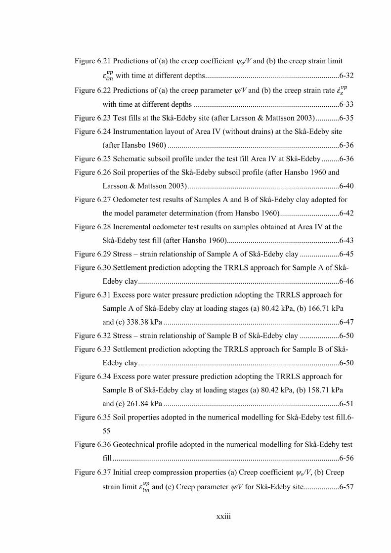
Figure 6.21 Predictions of (a) the creep coefficient o/V and (b) the creep strain limit

with time at different depths .................................................................... 6-32

Figure 6.22 Predictions of (a) the creep parameter /V and (b) the creep strain rate

with time at different depths .......................................................................... 6-33

Figure 6.23 Test fills at the Skå-Edeby site (after Larsson & Mattsson 2003) ............ 6-35

Figure 6.24 Instrumentation layout of Area IV (without drains) at the Skå-Edeby site

(after Hansbo 1960) ....................................................................................... 6-36

Figure 6.25 Schematic subsoil profile under the test fill Area IV at Skå-Edeby ......... 6-36

Figure 6.26 Soil properties of the Skå-Edeby subsoil profile (after Hansbo 1960 and

Larsson & Mattsson 2003) ............................................................................. 6-40

Figure 6.27 Oedometer test results of Samples A and B of Skå-Edeby clay adopted for

the model parameter determination (from Hansbo 1960) .............................. 6-42

Figure 6.28 Incremental oedometer test results on samples obtained at Area IV at the

Skå-Edeby test fill (after Hansbo 1960) ......................................................... 6-43

Figure 6.29 Stress – strain relationship of Sample A of Skå-Edeby clay .................... 6-45

Figure 6.30 Settlement prediction adopting the TRRLS approach for Sample A of Skå-

Edeby clay ...................................................................................................... 6-46

Figure 6.31 Excess pore water pressure prediction adopting the TRRLS approach for

Sample A of Skå-Edeby clay at loading stages (a) 80.42 kPa, (b) 166.71 kPa

and (c) 338.38 kPa ......................................................................................... 6-47

Figure 6.32 Stress – strain relationship of Sample B of Skå-Edeby clay .................... 6-50

Figure 6.33 Settlement prediction adopting the TRRLS approach for Sample B of Skå-

Edeby clay ...................................................................................................... 6-50

Figure 6.34 Excess pore water pressure prediction adopting the TRRLS approach for

Sample B of Skå-Edeby clay at loading stages (a) 80.42 kPa, (b) 158.71 kPa

and (c) 261.84 kPa ......................................................................................... 6-51

Figure 6.35 Soil properties adopted in the numerical modelling for Skå-Edeby test fill . 6-

55

Figure 6.36 Geotechnical profile adopted in the numerical modelling for Skå-Edeby test

fill ................................................................................................................... 6-56

Figure 6.37 Initial creep compression properties (a) Creep coefficient o/V, (b) Creep

strain limit and (c) Creep parameter /V for Skå-Edeby site .................. 6-57

xxiv

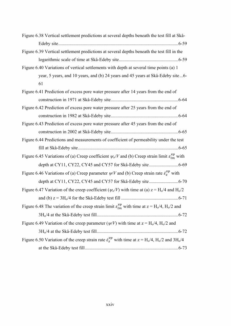
Figure 6.38 Vertical settlement predictions at several depths beneath the test fill at Skå-

Edeby site ....................................................................................................... 6-59

Figure 6.39 Vertical settlement predictions at several depths beneath the test fill in the

logarithmic scale of time at Skå-Edeby site ................................................... 6-59

Figure 6.40 Variations of vertical settlements with depth at several time points (a) 1

year, 5 years, and 10 years, and (b) 24 years and 45 years at Skå-Edeby site ... 6-

61


construction in 1971 at Skå-Edeby site .......................................................... 6-64





Figure 6.44 Predictions and measurements of coefficient of permeability under the test

fill at Skå-Edeby site ...................................................................................... 6-65

Figure 6.45 Variations of (a) Creep coefficient /V and (b) Creep strain limit with

depth at CY11, CY22, CY45 and CY57 for Skå-Edeby site ......................... 6-69

Figure 6.46 Variations of (a) Creep parameter /V and (b) Creep strain rate with

depth at CY11, CY22, CY45 and CY57 for Skå-Edeby site ......................... 6-70

Figure 6.47 Variation of the creep coefficient ( o/V) with time at (a) z = Ho/4 and Ho/2

and (b) z = 3Ho/4 for the Skå-Edeby test fill ................................................. 6-71

Figure 6.48 The variation of the creep strain limit with time at z = Ho/4, Ho/2 and

3Ho/4 at the Skå-Edeby test fill ...................................................................... 6-72

Figure 6.49 Variation of the creep parameter ( /V) with time at z = Ho/4, Ho/2 and

3Ho/4 at the Skå-Edeby test fill ...................................................................... 6-72

Figure 6.50 Variation of the creep strain rate with time at z = Ho/4, Ho/2 and 3Ho/4

at the Skå-Edeby test fill ................................................................................ 6-73

xxv

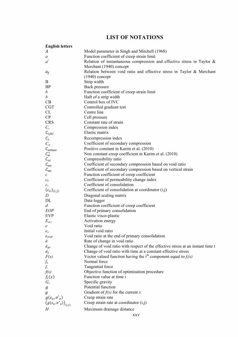
LIST OF NOTATIONS English letters

Model parameter in Singh and Mitchell (1968) a Function coefficient of creep strain limit a’ Relation of instantaneous compression and effective stress in Taylor &

Merchant (1940) concept Relation between void ratio and effective stress in Taylor & Merchant

(1940) concept B Strip width BP Back pressure b Function coefficient of creep strain limit b Haft of a strip width CB Control box of IVC CGT Controlled gradient test CL Centre line CP Cell pressure CRS Constant rate of strain Cc Compression index

Elastic matrix Recompression index

C Coefficient of secondary compression Positive constant in Karim et al. (2010)

Non constant creep coefficient in Karim et al. (2010) Compressibility ratio Coefficient of secondary compression based on void ratio Coefficient of secondary compression based on vertical strain

c Function coefficient of creep coefficient ck Coefficient of permeability change index cv Coefficient of consolidation

Coefficient of consolidation at coordinator (i,j) D Diagonal scaling matrix DL Data logger d Function coefficient of creep coefficient EOP End of primary consolidation EVP Elastic visco-plastic Eact Activation energy e Void ratio eo Initial void ratio eEOP Void ratio at the end of primary consolidation

Rate of change in void ratio Change of void ratio with respect of the effective stress at an instant time t

Change of void ratio with time at a constant effective stress F(x) Vector valued function having the ith component equal to fi(x) fn Normal force ft Tangential force f(x) Objective function of optimisation procedure

Function value at time i Gs Specific gravity

Potential function g Gradient of f(x) for the current x

Creep strain rate Creep strain rate at coordinator (i,j)

H Maximum drainage distance

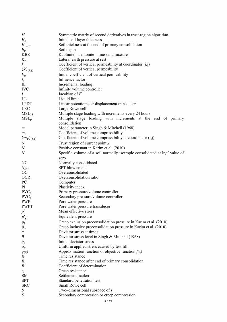
xxvi

H Symmetric matrix of second derivatives in trust-region algorithm Initial soil layer thickness

Soil thickness at the end of primary consolidation Soil depth

KBS Kaolinite – bentonite – fine sand mixture Ko Lateral earth pressure at rest k Coefficient of vertical permeability at coordinator (i,j)

Coefficient of vertical permeability Initial coefficient of vertical permeability

Iz Influence factor IL Incremental loading IVC Infinite volume controller Jacobian of F

LL Liquid limit LPDT Linear potentiometer displacement transducer LRC Large Rowe cell MSL24 Multiple stage loading with increments every 24 hours MSLp Multiple stage loading with increments at the end of primary

consolidation m Model parameter in Singh & Mitchell (1968) mv Coefficient of volume compressibility

Coefficient of volume compressibility at coordinator (i,j) N Trust region of current point x N Positive constant in Karim et al. (2010) N Specific volume of a soil normally isotropic consolidated at lnp’ value of

zero NC Normally consolidated NSPT SPT blow count OC Overconsolidated OCR Overconsolidation ratio PC Computer PI Plasticity index PVCp Primary pressure/volume controller PVCs Secondary pressure/volume controller PWP Pore water pressure PWPT Pore water pressure transducer p’ Mean effective stress

Equivalent pressure Creep exclusion preconsolidation pressure in Karim et al. (2010) Creep inclusive preconsolidation pressure in Karim et al. (2010)

q Deviator stress at time t Deviator stress level in Singh & Mitchell (1968)

qo Initial deviator stress Uniform applied stress caused by test fill

q(s) Approximation function of objective function f(x) R Time resistance Rs Time resistance after end of primary consolidation R2 Coefficient of determination rs Creep resistance SM Settlement marker SPT Standard penetration test SRC Small Rowe cell S Two–dimensional subspace of s

Secondary compression or creep compression

xxvii

Primary compression Surface settlement at time t

Su Undrained shear strength s Trial step of x Sliding velocity

T Absolute temperature Tv Unitless time factor TRRLS Trust-region reflective least squares t Elapsed loading time t’ Difference between and tc to Time parameter tc Time at conventional end of primary consolidation

Time corresponding to the instant time-line in Garlanger (1972) or reference time in Singh & Mitchell (1968)

te Equivalent time Extrapolated time corresponding to R = 0

Total loading time Visco-plastic (creep) time

tEOC Construction time tEOP Time at the end of primary consolidation U Degree of consolidation

Excess pore water pressure at coordinator (i,j) Initial excess pore water pressure in Taylor & Merchant (1940) Hydrostatic pore water pressure, initial equilibrium water pressure

ue Excess pore water pressure uei Initial excess pore water pressure (= z)

Excess pore water pressure at time t in Taylor & Merchant (1940) Total squares of difference between measured and predicted values

V Specific volume corresponding to eo v Specific volume of a soil at the normal stress p’ wo Initial water content wc, w Water content x Vector of variable

Measured data point at time i z Soil depth zt Compression per unit of layer thickness

Greek letters Trust region radius > 0

t Time step z Space step

Relationship between the logarithm of the preconsolidation pressure and the logarithm of the strain rate Model parameter in Singh & Mitchell (1968)

p Immediate settlement per unit of thickness and unit of load s Rate of secondary compression per unit thickness and load unit

Load increment z Applied stress increment

Fluidity parameter Unit weight of soil Unit weight of water

z Vertical strain

xxviii

zi Initial vertical strain Vertical strain at coordinator (i,j)

Average vertical strain at time t

Vertical elastic strain Vertical elastic strain at ’z = ’u Elastic plastic strain at

Vertical plastic strain Vertical reference strain at ’z

Vertical reference strain at ’z at coordinator (i,j) Vertical reference strain at ’zo Creep strain limit

Creep strain limit at coordinator (i,j)

Visco-plastic (creep) strain Strain rate Creep strain rate Elastic strain rate Visco-plastic strain rate Vertical visco-plastic (creep) strain rate

End of primary consolidation strain rate Vertical plastic strain rate

Elastic stiffness Slope of the normal isotropic consolidation line in the isotropic normal compression

/V Elastic plastic stiffness Coefficient of secondary compression by Taylor & Merchant (1940) * Modified creep parameter

Coefficient of viscosity Total vertical stress

’ij Stress state ’po Preconsolidation pressure before loading ’pc Preconsolidation pressure ’z Vertical effective stress

Vertical effective stress at coordinator (i,j) ’u Unit vertical effective stress (i.e. 1 kPa) ’zi Initial vertical effective stress ’zo EVP model parameter, vertical effective stress corresponding to

Final vertical effective stress Stress rate Rate of change in effective stress

Time parameter = 1 day c Difference between tc and tr o/V Creep coefficient /V Creep parameter

doctor of philosophy - opus at uts: home · pdf filein this thesis, a series of laboratory...

Documents