doc, what are my chances? · doc, what are my chances? 279 doc, ... san buenaventura (st....

Doc, What Are My Chances? 279

Doc, What Are My Chances?Joe MarascoPebble Beach, [email protected]

Ron DoerflerNaperville, ILhttp://[email protected]

Leif RoschierVantaa, [email protected]

IntroductionWhen a physician has to deliver bad news to a patient, the bottom-line

question is, “Doc, what are my chances?” The doctor’s answers are thenusually couched in the language of probability.Recently, both patients and insurance companies have become more

questioning, because theywant tounderstandthedoctor’s reasoning. Whatpersists is an explanation gap, the distance between the doctor’s best as-sessment and the patient’s comprehension of both the probability and howit was obtained.We seek to reveal the logic behind the medical diagnostic decision-

making process and arm the patient with the appropriate vocabulary. Be-cause decisions hinge on probabilities—“we’ll proceed to this treatment ifwe can ascertain that there is at least a 50% chance you have the disease”—we demonstrate how the numbers are determined. This approach removesthe fuzziness from the process, and the required arithmetic is not intimidat-ing when taken one step at a time. To demonstrate the method, we work asample problem from start to finish.We illustrate how a graphical solution called a nomogram [Doerfler 2009]

delivers numerical results easily. Moreover, nomograms can offer advan-tages over other computational methods; an appendix gives a comparison.

TheUMAP Journal 32 (4) (2011) 279–298. c�Copyright 2011 byCOMAP, Inc. All rights reserved.Permission to make digital or hard copies of part or all of this work for personal or classroom useis granted without fee provided that copies are not made or distributed for profit or commercialadvantage and that copies bear this notice. Abstracting with credit is permitted, but copyrightsfor components of this work owned by others than COMAPmust be honored. To copy otherwise,to republish, to post on servers, or to redistribute to lists requires prior permission from COMAP.

280 The UMAP Journal 32.4 (2011)

A Hypothetical Deadly DiseaseSuppose that 5% of the population of San Buenaventura1 has MacGuf-

fin’s disease2. Untreated, 80% perish within two years; but a 95% effectivetreatment exists. What would you do? One approach is to do nothing. SanBuenaventura’s population is 100,000, so 80% of the 5,000 peoplewho havethe disease, or 4,000, die within two years. This constitutes our baseline.The opposite alternative is to treat everyone. We now need to know:• What is the probability of survival for someone who is treated but doesnot have the disease?

• What is the cost of the treatment? Ultimately, we want to save as manylives as possible while minimizing the cost per life saved.

Addressing the first concern, let’s suppose that out of 1,000 healthy peoplewho are treated, 5 die from the treatment. The survival rate for the healthyuntreated is 100% because throughout this analysis we ignore deaths thatare not due toMacGuffin’s disease. Table 1(a) summarizes all possibilities,with the shaded cells in the 2⇥ 2 arrays indicating incorrect actions.

No TreatmentIn Table 1(b), we use the do-nothing scenario to illustrate how to com-

pute overall survival. We do the multiplication “box-by-box” and thensum the numbers in the right-hand 2⇥ 2 array to get the total number ofsurvivors. That total is then divided by the population to get the overallsurvival probability.

Treat EveryoneTable 1(c) shows the treat-everyone scenario. Against the 4,750diseased

who are saved, 475 healthy people die from unneeded treatment. Remem-ber that 20% of the original 5,000 diseased, or 1,000, would have survivedwithout treatment; so the net gain is 3,275 lives. To achieve this objective,we treat all 100,000 people. Assuming that the cost of the treatment is $100per person, we spend $10 million and the cost per life saved is $3,053.

1This San Buenaventura is imaginary and the reader should make no association with MissionSan Buenaventura (St. Bonaventure) in Ventura, CA, nor with towns of that name in Mexico andBolivia, nor with the university of that name in Cali, Colombia.

2A MacGuffin is a plot device, often an object, that is initially the central focus of a film orstory but then declines in importance. The term was invented by Alfred Hitchcock in connectionwith his film The 39 Steps; later examples include the Maltese falcon in the film of the same name,the meaning of “rosebud” in Citizen Kane, and the mineral “unobtainium” in Avatar. The termwas also used by the now-defunct Macguffin Game company to denote a design object that forcesinteractivity. Predating the term itself is literary use of such a device, as with the gold in the operaDas Rheingold or the Sampo in the Finnish epic Kalevala. (adapted fromWikipedia [2011])


Table 1.Two-year survival probabilities for MacGuffin’s disease under various scenarios.

2

Table 1: Two-‐year survival probabilities for MacGuffin's Disease under various scenarios

Survival Percentage Healthy Diseased Untreated 100.0% 20.0% Treated 99.5% 95.0%

(a) Survival Percentages used in tables (b), (c), (d), and (e)

Shaded cells in 2x2 always indicate an incorrect action

Survival Percentage Number in Population Number Surviving Healthy Diseased Healthy Diseased Healthy Diseased

Untreated 100.0% 20.0% x

Untreated 95,000 5,000 =

Untreated 95,000 1,000 Treated 99.5% 95.0% Treated 0 0 Treated 0 0

Prevalence 5% Overall Survival Probability 96.00% (b) Treat No One (Baseline) Lives Saved 0

Cost per Life Saved N/A


Untreated 100.0% 20.0% x Untreated 0 0 = Untreated 0 0 Treated 99.5% 95.0% Treated 95,000 5,000 Treated 94,525 4,750

Prevalence 5% Overall Survival Probability 99.28% (c) Treat Everyone Lives Saved 3,275

Cost per Life Saved $3,053



Untreated 95,000 0 =

Untreated 95,000 0 Treated 99.5% 95.0% Treated 0 5,000 Treated 0 4,750

Prevalence 5% Overall Survival Probability 99.75% (d) Treat Perfect Test Positives Lives Saved 3,750

Cost per Life Saved $133



Untreated 90,250 4,750 =

Untreated 90,250 950 Treated 99.5% 95.0% Treated 4,750 250 Treated 4,726 238

Prevalence 5% Overall Survival Probability 96.16% (e) Treat Useless Test Positives Lives Saved 164

Cost per Life Saved $3,049

In Table 1(b) we use the do-‐nothing scenario to illustrate how to compute overall survivability. We do -‐by-‐

of survivors. That total is then divided by the population to get the overall survival probability.

Table 1(c) shows the computation for the treat-‐everyone scenario. Against the 4,750 diseased who are saved, 475 healthy people die from unneeded treatment. Remember that 20% of the original 5,000 diseased would have survived without treatment, so the net gain is 3,275 lives. To achieve this objective, we treat all 100,000 people. Assuming that the cost of the treatment is $100 per person, we spend $10 million and the cost per life saved is $3,053.

A Perfect Diagnostic TestTo treat more selectively, we must perform a diagnostic test or a series

of diagnostic tests to try to determine whether a patient has the disease.The test itself has the potential for side effects, risks, and incremental cost,which we consider negligible compared to their treatment analogues.Table 1(d) shows the results for a test that is never wrong: All patients

who have the disease test positive, and all patients who don’t have it testnegative. We then administer treatment based on this result. No healthypeople perish because of unneeded treatment; and since we administertreatment to diseased patients only, we minimize the cost per life saved,which plummets from $3,053 to $133.


A Useless Diagnostic TestWhile there is only one conceptually perfect test, there are many useless

ones. In Table 1(e), we assume that 5% have the disease, and 5% at randomtest positive (not necessarily the same 5%!). We treat the 5% who testpositive, with no discrimination between diseased and healthy. The resultsare only slightly better than the do-nothing approach of Table 1(b): Theoverall survival probability is 96.16% vs. 96.00%. Only 164 lives are saved,at a cost of $3,049 each; we treat fewer people and save fewer lives. (Theminuscule $4 difference in cost per life saved relative to the treat-everyonescenario of Table 1(c) is due to rounding the number of lives saved from163.75 to 164. We avoid fractional lives and deaths.) Although the total costof the treatment program goes down to $500,000, the cost per life saved isthe same as in the treat-everyone scenario, because the test did not yieldany new information.We have a 9.5% error rate for this test: It delivers the wrong result in

9,500 out of 100,000 tests:• 5% of the 95,000 healthy people (4,750), plus• 95% of the 5,000 with the disease (another 4,750).Although it is correct over 90% of the time, the test is useless because itprovides no discrimination; there is a 5% probability of testing positiveregardless of whether one has, or does not have, MacGuffin’s disease.Using the same survival percentages, the trends shown with a pretest

probability of 5% persist when we change it to 10% or 20%.

Real-World TestsAll real-world tests fall somewhere between perfect and useless. A test

can never tell with certainty that a patient has the disease or does not. Itcan only increase our estimate of the probability that the patient has thedisease if the test result is positive, or decrease our estimate if the resultis negative. Testing matters, both in terms of lives saved and cost per lifesaved. However, there is a wide range of improvement as one progressesfromuseless tests to nearer-to-perfect tests. The argument for testinghingescritically on the discriminating power of the test.

Role of the PhysicianUp to this point, we have ignored the role of the physician. A random

resident of San Buenaventura has a probability of MacGuffin’s of 5%. Butthe physician always knows more, because he or she takes a history (whichincludes prior conditions as well as familial factors) and checks for symp-toms.


Suppose that using all the available information, the physician estimatesthat for a particular patient the probability is 30%, or six times the average for theentire population.

Threshold for TreatmentSuppose that treatment (whichmay have nonfatal but undesirable side-

effects for all those treated, diseased or not) is applied only if we believe that thepatient has at least a 50% probability of having the disease. This threshold candepend on many factors—it can vary from disease to disease, from treat-ment to treatment, and from patient to patient—there is nothing magicalabout 50%.Since the pretest estimate of 30% for our hypothetical patient is less than

the treatment threshold of 50%, the physician can attempt to refine the esti-mate by performing a test, which will either raise the patient’s probabilityof having MacGuffin’s (for a positive test result) or lower it (for a negativeresult).Should the physician order such a test? (We ignore its cost, assuming

that it is negligible compared to that of the treatment.)

Testing LogicRecall that the left-hand portion of the tables (the survival percentages)

tells the effectiveness of the treatment. Themiddle part determineswho getstreated; we do tests so as to alter the relative populations in those cells.Table 2 compares a perfect test with a useless test. The shaded cells in theright-hand portion indicate the cases where we go wrong.

Table 2.Population for perfect vs. useless tests.

4

Recall that the left hand part of the tables (the survival percentages) tells us the effectiveness of the treatment, while the middle part determines who gets treated. We do tests to alter the population of those cells. Compare the perfect test with the useless test in Table 2.

Table 2: Population for perfect vs. useless tests

Population Table, Perfect Test Population Table, Useless Test Healthy Diseased Healthy Diseased Untreated 95,000 0 Untreated 90,250 4,750 Treated 0 5,000 Treated 4,750 250

The shaded cells in right hand portion indicate the cases where we have gone wrong. Table 3 shows that when we treat the disease that is not present, we are depending on a test that issued a false positive report: It told us the disease was present when it was not. When we fail to treat the disease based on the test, it was because of a false negative: The disease was present, but the test missed it.

Table 3: Test characterization 2x2

Healthy Diseased Negative Test Result True Negatives False Negatives Positive Test Result False Positives True Positives

The power of a test lies in its ability to minimize these two types of errors and in its ability to raise the

our example the doctor estimated the pretest probability at 30%, and the treatment threshold is 50%. Any test powerful enough to raise the estimate of the probability from 30% to 50% or more is useful, because it affects our course of action. On the other hand, a test that raises our probability estimate from 30% to only 40% is not worth doing, because even if the result comes back positive, we are still below the treatment threshold.

Note that if the physician is conservative, he may do a test to validate his initial estimate even if it is above the treatment threshold. In the case of a pretest probability of 70%, he would seek a test powerful enough to cause the posttest probability to dip below 50% if the result comes back negative.

Figure 1 illustrates the overall process.

The numbers in the four boxes of Table 3, obtained through previous experience with the test, completely characterize its discriminatory power. Lacking them, we rely on derived numbers.

The most useful are Likelihood Ratios.4 One called LR+ indicates how much our pretest probability increases if the test result is positive. An LR+ of 1 represents the useless test, and as LR+ increases, the test becomes more discriminatory. An LR+ of 10 is considered to be quite good; a perfect test approaches infinity. We take LR+ as our measure of the power of the test.5

If the test result is negative, another number, LR-‐, allows us to compute how much the posttest probability of disease has decreased which is useful in refuting confirmatory bias.

Table 3 characterizes the situations of Table 2:• Whenwe give treatment but the disease is not present, the test has issueda false positive report that the disease was present when it was not.

• When, based on the test, we fail to treat the disease when it is present,it was because of a false negative: The disease was present, but the testmissed it.The power of a test lies in its abilities

• to minimize these two types of errors (false positive and false negative), and• to raise the physician’s pretest probability estimate.


Table 3.Test characterization 2⇥ 2.

4

Recall that the left hand part of the tables (the survival percentages) tells us the effectiveness of the treatment, while the middle part determines who gets treated. We do tests to alter the population of those cells. Compare the perfect test with the useless test in Table 2.

Table 2: Population for perfect vs. useless tests

Population Table, Perfect Test Population Table, Useless Test Healthy Diseased Healthy Diseased Untreated 95,000 0 Untreated 90,250 4,750 Treated 0 5,000 Treated 4,750 250

The shaded cells in right hand portion indicate the cases where we have gone wrong. Table 3 shows that when we treat the disease that is not present, we are depending on a test that issued a false positive report: It told us the disease was present when it was not. When we fail to treat the disease based on the test, it was because of a false negative: The disease was present, but the test missed it.

Table 3: Test characterization 2x2

Healthy Diseased Negative Test Result True Negatives False Negatives Positive Test Result False Positives True Positives

The power of a test lies in its ability to minimize these two types of errors and in its ability to raise the

our example the doctor estimated the pretest probability at 30%, and the treatment threshold is 50%. Any test powerful enough to raise the estimate of the probability from 30% to 50% or more is useful, because it affects our course of action. On the other hand, a test that raises our probability estimate from 30% to only 40% is not worth doing, because even if the result comes back positive, we are still below the treatment threshold.

Note that if the physician is conservative, he may do a test to validate his initial estimate even if it is above the treatment threshold. In the case of a pretest probability of 70%, he would seek a test powerful enough to cause the posttest probability to dip below 50% if the result comes back negative.

Figure 1 illustrates the overall process.

The numbers in the four boxes of Table 3, obtained through previous experience with the test, completely characterize its discriminatory power. Lacking them, we rely on derived numbers.

The most useful are Likelihood Ratios.4 One called LR+ indicates how much our pretest probability increases if the test result is positive. An LR+ of 1 represents the useless test, and as LR+ increases, the test becomes more discriminatory. An LR+ of 10 is considered to be quite good; a perfect test approaches infinity. We take LR+ as our measure of the power of the test.5

If the test result is negative, another number, LR-‐, allows us to compute how much the posttest probability of disease has decreased which is useful in refuting confirmatory bias.

In our example, the physician estimated the pretest probability at 30%,and the treatment threshold is 50%. Any test powerful enough to raise theestimate from 30% to 50% or more is useful, because it affects our course ofaction. On the other hand, a test that raises the estimate from 30% to only40% is not worth doing, because even if the result comes back positive, weare still below the treatment threshold.A conservative physician may do a test to validate the initial estimate

even if it it was above the treatment threshold. For example, in the case of apretest probability of 70%, thephysicianwould seek a test powerful enoughto cause the posttest probability to dip below 50% if the result comes backnegative.Figure 1 illustrates the overall process.

I

I

I

I

I

Figure 1. Decision process based on initial workup plus additional test.


Likelihood RatiosThe numbers in the four boxes of Table 3, obtained for a real-world test

through previous experience, completely characterize its discriminatorypower. Lacking them, we must rely on derived numbers, such as likelihoodratios [Dujardin et al. 1994]. One called LR+ indicates howmuch our pretestprobability increases if the test result is positive: An LR+ of 1 represents auseless test; and as LR+ increases, the test becomes more discriminating.An LR+ of 10 is considered quite good; for a perfect test, LR+ approachesinfinity. We take LR+ as our measure of the power of the test.The likelihood ratio is an odds multiplier. The relationship is called

Bayes’ Theorem:

Bayes’ Theorem. The posttest odds equal the pretest odds times thevalue of LR+:

posttest odds = (pretest odds)⇥ LR+.

However, the relationship between probabilities and odds is that

odds = probability1� probability.

Starting with a pretest probability, you first convert to pretest odds,multiply by LR+, and then convert from posttest odds back to posttestprobability.If the test result is negative, another number, LR�, allows us to com-

pute how much the posttest probability of disease has decreased—whichis useful in refuting confirmatory bias. A similar computation applies.

A Graphical CalculatorOur Figure 2, a member of a family of geometric calculators known as

nomograms, performs the computation of posttest probability without needfor a computer (see Doerfler [2009] for further examples of nomograms).In Figure 2 (reproduced at a larger size in the foldout at the back of this

issue3), let’s continue to assume a pretest probability of 30%, and supposethat the test has LR+ = 2.8. Although Figure 2 appears complex, the key toits use is to focus only on the scales of immediate interest. The tradeoff forthe complexity is that this figure allows the correlation of all the relevantfactors in a single graphic.

3High-quality hard copies of the nomograms of Figures 2 and 4, in color and in varioussizes useful to practitioners, can be obtained from http://www.modernnomograms.com . Read-ers interested in creating their own nomograms using the free PyNomo software should seehttp://www.pynomo.org .


Posttest Odds For Posttest Odds Against

Pretest Odds Against Pretest Odds For

Speci!city of Test for LR + Sensitivity of Test for LR "

Speci!city of Test for LR " Sensitivity of Test for LR +

LR + LR "

Posttest Probability Predictor

Positive Test Result Negative Test Result

Posttest Probability

Pretest Probability

e for LR +f for LR "

e for LR "f for LR +

DiseasedHealthyTN FN

TPFPf = FP/TN e = FN/TP

Negative Test ResultPositive Test Result

Critical Ratio

Test Characterization

Figure 2. Bayes’ theorem nomogram.

Start at the bottom of the circle and locate the 30% pretest probabilitypoint. On the horizontal LR+ scale in the middle of the figure (positive testresult), find the value of 2.8. Extending a line through these two points tothe top of the circle yields a posttest probability of just under 55%. Thisprocess is shown schematically in the upper left part of Figure 3. Since55% is greater than the treatment threshold of 50%, we would do this testand proceed to treatment if the result is positive. You can make the testdecision as quickly as you can draw a straight line; the test result thenunambiguously determines the course of treatment.The first tool of this kind formedical purposeswas put forth byDr. Terry

Fagan [1975]. Today, manyphysicianswould use a computer application to


Positive Test ResultLR+ Known

Positive Test ResultLR+ Unknown

Negative Test Result Negative Test Result





LR + LR "



Pretest Probability


e for LR "f for LR +Posttest Odds For Posttest Odds Against




LR + LR "



Pretest Probability







LR + LR "



Pretest Probability


e for LR "f for LR +Posttest Odds For Posttest Odds Against




LR + LR "



Pretest Probability



LR+ LR+

LR" LR"

Figure 3. Using the Bayes’ theorem nomogram of Figure 2with the sample problem data.

performsuch calculations, perhaps even accomplishing it on a smartphone.We can also use Figure 2 to work backwards. If you draw a line from

the posttest probability (treatment threshold) of 50% through the point rep-resenting a test with an LR+ of 2.8, you discover that such a test should notbe performed if the pretest probability is less than about 26%.


Sensitivity and SpecificitySometimes the value of LR+ for a particular test is not stated. Two other

numbers suffice: the sensitivity and specificity:• The sensitivity of a test reflects the ability of the test to detect the diseasewhen it is present. It is the ratio of true positives to all diseasedpeople, thatis, the ratio of true positives to the sum of the true positives and the falsenegatives. Highly sensitive tests risk having a high false positive rate;in an attempt to detect as many instances as possible, the test inevitablystarts to “catch” things it shouldn’t.

• The specificity of a test is the ability of the test to establish that a personwithout the disease will test negative. It is the ratio of true negatives toall healthy people, that is, the ratio of true negatives to the sum of thetrue negatives and the false positives. Highly specific tests risk missingtrue positives in their attempt to minimize false positives; hence, thereis usually a tradeoff between high sensitivity and high specificity.For a short and easy-to-follow explanation of the relationship between

likelihood ratios and sensitivity and specificity, see Attia [2003].Both sensitivity and specificity range from 0 to 1, with the higher num-

bers being better. The formula for LR+ is:

LR+ = sensitivity1� specificity,

which means that as the specificity approaches 1, LR+ can become verylarge.

In practice, the general rule is:• A highly sensitive test with a negative result is good at ruling out thedisease, which makes the test useful for screening.

• Conversely, a highly specific test with a positive result is good at rulingin the disease, which makes it valuable for confirmation.

Likelihood Ratios from Sensitivity Plus SpecificityThe combination of sensitivity and specificity permit the computation

of both LR+ and LR�.Once again, we use Figure 2 to perform the calculation in the example

below.Enabling Figure 2 to handle this calculation of LR+ and LR� from sen-

sitivity and specificity is our improvement on Fagan’s original work. Ourgraphical layout is also different; 10 different variables are correlated in thisone diagram:


• 4 for pretest and posttest probability and odds,• 2 for LR+ and LR�,• 2 for the sensitivity and specificity of the test, and• 2 for e and f , two ratios that enable computation starting from the 2⇥ 2test characterization matrix.

Figure 3 supplies four small figure examples as usage reminders.Example. Suppose that we have a sensitivity of 0.17 and a specificityof 0.94; we locate in Figure 2 the sensitivity on the right-hand portionof the lower ellipse, and the specificity on the left-hand portion of theupper ellipse. Connecting these two values with a straight line yieldsan LR+ of 2.8, the same as calculated earlier. Computing the posttestprobability from the pretest probability now proceeds as before. Thistwo-step process is shown schematically in the upper right part ofFigure 3.If the test result is negative, Figure 2 demonstrates that the proba-

bility drops from 30% to 27%. LR� is defined as

LR� = 1� sensitivityspecificity

.

The value of LR� for this sensitivity and specificity is 0.89. Thesemanipulations are shown schematically at the lower right of Figure 3.Note that if the pretest probability had been 70%, a negative test resultlowers theposttestprobability to about68%, so this test is notpowerfulenough to be useful in excluding the disease (see Figure 1).Every test has a cutoff value that determines whether the result is pos-

itive or negative, and the values of LR and the sensitivity/specificity pairdepend on the cutoff value chosen. Sometimes the relationship leads toa spectrum of likelihood ratios—either discrete values or a continuousdistribution—that depends on the cutoff selected for the test. In such a situ-ation, you can choose the cutoff needed to achieve the treatment threshold.If, on the other hand, no likelihood ratios or sensitivity/specificity pairs areavailable, then the protocol breaks down.

Rare DiseasesFor a disease with a very low pretest probability, say 1% or less, there

may not be a single test powerful enough to get us over the treatmentthreshold. Figure 2 also presents a problem: The large values required ofLR+ fall in a very compressed part of that scale. Figure 4 handles the caseof low pretest probabilities and high values of LR+.With a pretest probability of 1%, and two tests:


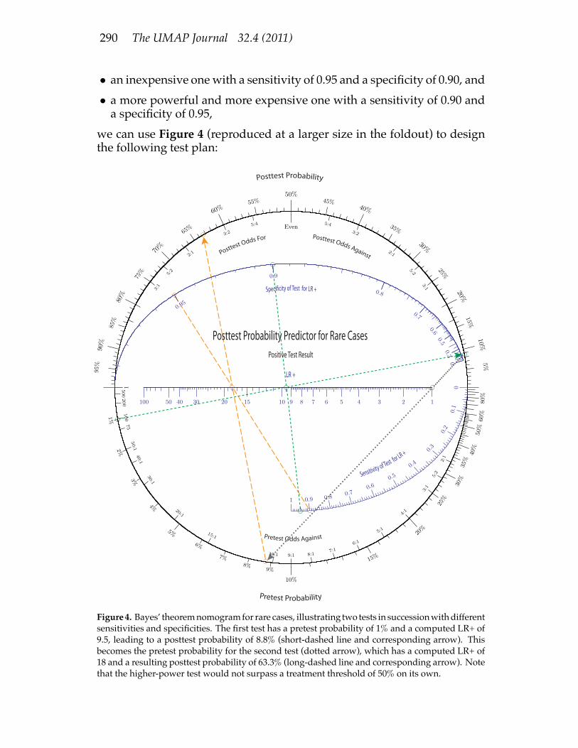
• an inexpensive onewith a sensitivity of 0.95 and a specificity of 0.90, and• a more powerful and more expensive one with a sensitivity of 0.90 anda specificity of 0.95,

we can use Figure 4 (reproduced at a larger size in the foldout) to designthe following test plan:


Sensitivity of Test for LR +


Pretest Probability

Posttest Probability Predictor for Rare CasesPositive Test Result

LR +

Speci!city of Test for LR +

Pretest Odds Against

Figure4. Bayes’ theoremnomogramfor rare cases, illustrating two tests in successionwithdifferentsensitivities and specificities. The first test has a pretest probability of 1% and a computed LR+ of9.5, leading to a posttest probability of 8.8% (short-dashed line and corresponding arrow). Thisbecomes the pretest probability for the second test (dotted arrow), which has a computed LR+ of18 and a resulting posttest probability of 63.3% (long-dashed line and corresponding arrow). Notethat the higher-power test would not surpass a treatment threshold of 50% on its own.


• Determine the LR+ of the first test as before: (0.95, 0.9) ! LR+ = 9.5;• Do the inexpensive test first: pretest probability = 1%, LR+ = 9.5 !posttest probability = 8.8%;

• If the test result is positive:– Determine the LR+ of the second test: (0.90, 0.95)! LR+ = 18.– Draw an arrow from the posttest probability of 8.8% for the first testdown through an LR+ of 1, reaching 8.8% on the pretest scale. (ForLR+ = 1, pretest and posttest probabilities are the same; this actionjust sets the pretest probability for the second test to be the posttestprobability from the first test.).

– Do the expensive test: pretest probability = 8.8%, LR+ = 18 !posttest probability of 63.3%,which is above our treatment thresholdof 50%.

Themore sensitive test is less powerful than the one that ismore specific.In this case, neither test alone will get us over the treatment threshold, butboth tests yielding positive results will. Doing the tests in either orderobtains the same result, so it makes sense to do the inexpensive test first.Figure 4 has the advantage of a higher range of LR+ values and much

better resolution for both the pretest probability and LR+ scales. It does nothave scales for LR� because in the case of a rare disease, a negative test isalmost always conclusive. Although we consider only LR+ for this case,with some gymnastics Figure 4 can be employed for LR�.

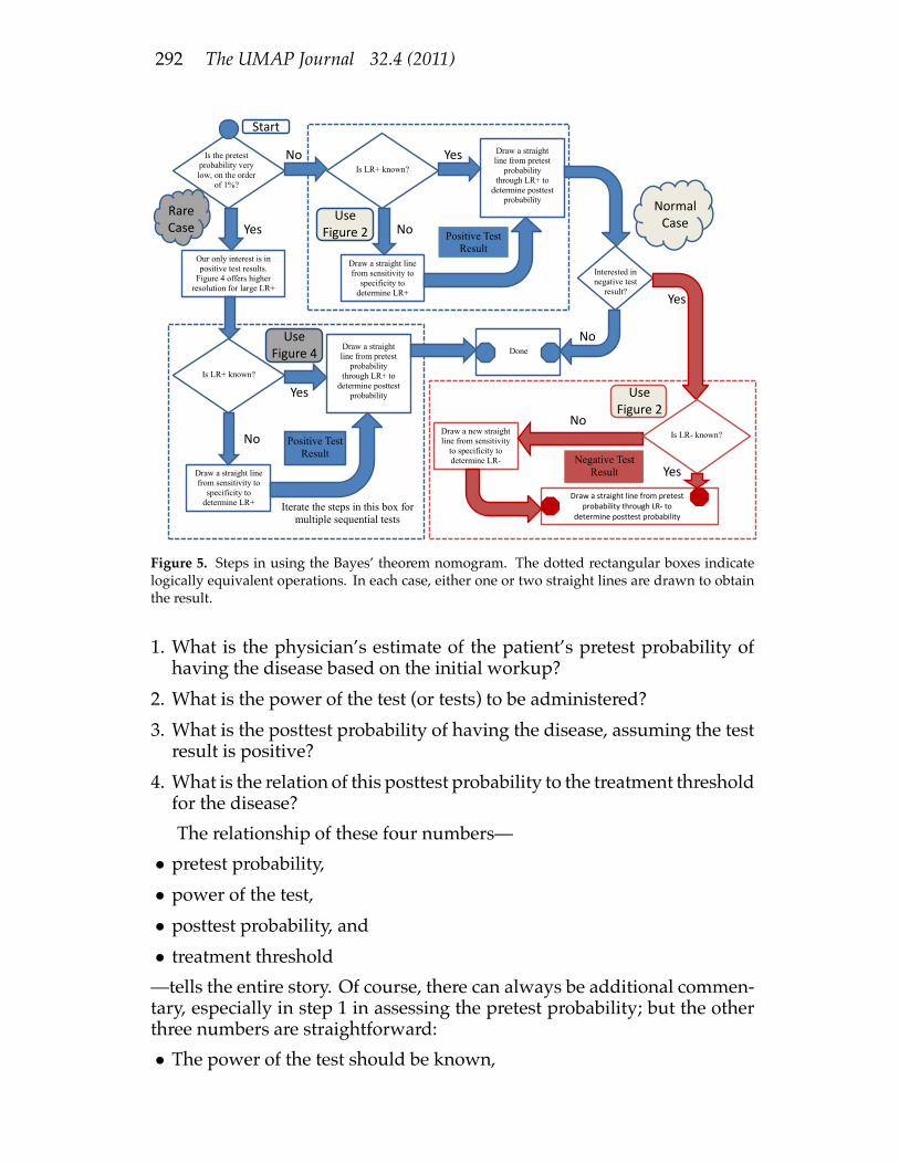
The Decision ProcessFigure 1 can be adapted tomap the decision steps for a chain ofmultiple

tests. Themultiple test approachmayalso be employedwithFigure 2whenmore convenient. Designing an optimum test protocol involving multipletests can be subtlewhen there are several tests to choose from, each ofwhichhas a different cost-to-power ratio. Our nomograms help.Figure 5 shows the decision criteria for the two figures and the steps

involved for each.We’ve divided the treatment decision process into two parts:

• First, the physician uses experience to estimate the probability that apatient has the disease.

• If a test can provide additional information, the physician then assesseswhether it is powerful enough to change the treatment decision; thatanswer determines whether to administer the test or not.The nomograms allow the posttest probability to be determined quickly

and accurately if either of two discriminatory metrics are known: the like-lihood ratios, or both the sensitivity and specificity of the test.The protocol consists of questions that can be answered numerically:


Our only interest is in positive test results.

Figure 4 offers higher resolution for large LR+

OOI

I Is LR+ known?

Draw a straight line from sensitivity to

specificity to determine LR+

I

Draw a straight line from pretest

probability through LR+ to

determine posttest probability

I

Is the pretest probability very low, on the order

of 1%?

Draw a straight line from sensitivity to

specificity to determine LR+

Draw a straight line from pretest

probability through LR+ to


Is LR+ known?

Interested in negative test

result?

Done

Draw a new straight line from sensitivity

to specificity to determine LR-

I Is LR- known?

Draw a straight line from pretest probability through LR-‐ to


Figure 5. Steps in using the Bayes’ theorem nomogram. The dotted rectangular boxes indicatelogically equivalent operations. In each case, either one or two straight lines are drawn to obtainthe result.

1. What is the physician’s estimate of the patient’s pretest probability ofhaving the disease based on the initial workup?

2. What is the power of the test (or tests) to be administered?3. What is the posttest probability of having the disease, assuming the testresult is positive?

4. What is the relation of this posttest probability to the treatment thresholdfor the disease?The relationship of these four numbers—

• pretest probability,• power of the test,• posttest probability, and• treatment threshold—tells the entire story. Of course, there can always be additional commen-tary, especially in step 1 in assessing the pretest probability; but the otherthree numbers are straightforward:• The power of the test should be known,


• the posttest probability is then a graphical computation, and• the treatment threshold was established beforehand.The decision to test, and to treat if the result is positive, is straightforward.There are two benefits to this approach:

• The patient and the physician can proactively lay out a diagnostic planthatmakes sense to both of themand to otherswhoneed to concur. Crispdecisionpoints and clear criteria are known from thebeginning. It is easyto understand why a given test (or tests) will be performed or not, andthe bearing those tests have on the treatment plan.

• Retrospectively, there is a post-treatment quantitative evidentiary recordthat benefits everyone: patient, physician, hospital administrator, in-surer, and—in a case where good decisions nonetheless lead to pooroutcomes—the attorneys for both sides. In addition to knowing whatwas done (or not done), there is an understanding of why it was done(or not done).The rationale for testing is that it allows the more selective treatment of

anentirepopulation. However,wecanachieve thedesiredcost-benefitratioonly by performing the right tests; the discriminatory power of the test isthe linchpin of the argument. By providing a simple yet powerful graphicaltool that bridges the computational gap between the pretest probability andthe posttest probability, we endeavor to bring discriminatory power intoprominence and encourage its use in the diagnostic process.Real-Life Example: The YouTube video “The PSA test—What youneed to know” [Health Dialog 2010] considers the prostate-specificantigen (PSA) test for prostate cancer. We learn in the video that of100 males over the age of 50, 8 will test positive (PSA > 4) and 92 willtest negative (PSA 4). Of the 8who test positive, 3 are true positivesand 5 are false positives. Of the 92 men who test negative, 15 haveprostate cancer; these are false negatives. Overall, 18 of the 100 (18%)have prostate cancer at the time of testing.Figure 6 on the next page shows these numbers in the standard

format of Table 3, along with the calculation of two new quantities, eand f .Referringonce again toFigure 2, wenote that thesevalues for e and

f yield a sensitivity of 0.17 and a specificity of 0.94, which correspondto an LR+ of 2.8 and an LR� of 0.89—these are exactly the numbersthat we used in our example. (You can use Figure 4 to get betterresolution for LR+.) But we also know that without any other priorknowledge, thepretest probability for this cohort is 18%, because thereare 18 men—3 who will test positive and 15 who will test negative—who have the disease. Our nomogram tells us that an 18% pretestprobabilityanda testwithanLR+of2.8will yieldaposttestprobability


Figure 6. Computation of e and f from the 2⇥ 2 test characterization matrix.

of only 38%, which is less than even odds. Although this test yieldsthe correct result 80% of the time, it is not powerful (discriminating)enough and should not be routinely done. Starting from 18%, oneneeds a test with an LR+ of about 4.6 to get to 50%.We chose the numbers for our nomogram example to match the data in

the PSA-screening video in order to make the point that the tools allow usto say more than “the test isn’t perfect”: They give us an idea of howmuchit would have to be improved to be more useful. (However, we emphasizethat MacGuffin’s disease is imaginary and is not prostate cancer.)The conclusion not to routinely screen using the PSA test appears to be

consistent with current guidelines of the American Cancer Society [2011a].(A differing advisory for African-American men is consistent with theirhaving a higher-than-averagepretest probability, so that a positive outcomewould put them above a treatment threshold [American Cancer Society2011b].)

How the Nomogram Is UsefulLooking at Figure 6, note that if you know nothing other than that

the patient is a member of the overall cohort, the probability of havingprostate cancer is simply obtained from the sum of the numbers in thesecond column. That yields 18 diseased out of 100 total, for 18%.But Bayes’ theorem says that if you know that the test result is positive,

then the probability of having prostate cancer is simply computed from thesecond row, yielding 3 out of a total of 8, or 37.5%. Similarly, if you knowthat the test result is negative, the probability of having prostate cancer is


simply computed from the first row, giving a result of 15 out of a total of92, or 16.3%.These answers are (of course) identical to those obtained by the nomo-

graphic analysis. The reason why the nomogram is useful is that althoughthe Bayes’ theorem answers are directly obtained from the 2 ⇥ 2 matrix,they hold only for a prior probability of 18%. If the physician assesses adifferent prior probability, then you need the values of e and f to computethe posttest probability for that specific pretest (prior) probability.Normally, you do not have the 2⇥ 2matrix, so that you need to do the

computation from specificity and sensitivity, or from the likelihood ratios.When you have the 2 ⇥ 2 matrix, you can read off the answer directlywithout elaborate computation, if you assume that the prior probability isjust the probability of someone in the cohort having the disease before anytesting is done. We provide a way to get the other parameters from the2⇥ 2 matrix, reasoning that there are cases where the pretest probabilitywill be different and thus other values will come into play.What it boils down to is that the nomogram is most valuable when you

have only the secondary data. However, we felt it useful to include on thenomogram also the case where you have the information in “raw form,”that is, in the form of the values in the 2⇥ 2matrix. Note that e and f are insome sense surrogates for the sensitivity and specificity, a fact that is clearfrom their sharing the same real estate on the nomogram. The differentscales just express the transformation equations between the two sets ofparameters in a visual way.The Appendix makes a general comparison of the use of a nomogram

vs. solution via computer.

Authors’ NoteHigh-quality hard copies of the nomograms of Figures 2 and 4, in

color and in various sizes useful to practitioners, can be obtained fromhttp://www.modernnomograms.com . Readers who are interested in au-tomating the creation of their own nomograms using the free PyNomosoftware should see http://www.pynomo.org .


ReferencesAmerican Cancer Society. 2011a. American Cancer Society recommenda-

tions for prostate cancer early detection.http://www.cancer.org/Cancer/ProstateCancer/MoreInformation/ProstateCancerEarlyDetection/prostate-cancer-early-detection-acs-recommendations .Last Medical Review: 12/01/2010. Last Revised: 10/12/2011.

. 2011b. What are the risk factors for prostate cancer?http://www.cancer.org/Cancer/ProstateCancer/MoreInformation/ProstateCancerEarlyDetection/cancer-early-detection-risk-factors-for-prostate-cancer .Last Medical Review: 12/01/2010. Last Revised: 10/12/2011.

Attia, J. 2003. Moving beyond sensitivity and specificity: Using likelihoodratios to help interpret diagnostic tests. Australian Prescriber (26) 5: 111–113.

Doerfler, Ron. 2009. The lost art of nomography. The UMAP Journal 30 (2):457–493.

Dujardin, B., J. Van den Ende, A. Van Gompel, and J.P. Unger. 1994. Likeli-hood ratios: A real improvement for clinical decisionmaking? EuropeanJournal of Epidemiology 10 (1): 29–36.

Fagan, T.J. 1975. Letter: Nomogram for Bayes’s Theorem. New EnglandJournal of Medicine 293 (5): 257.

Health Dialog. 2010. The PSA test—What you need to know. Video, 1:24min. http://www.youtube.com/watch?v=ZJS_jskR39k . Uploaded25 February 2010.

Wikipedia. 2011. MacGuffin. http://en.wikipedia.org/wiki/MacGuffin .

AcknowledgmentsThe authors would like to thank the editor, Paul Campbell of Beloit Col-

lege, for first suggesting creation of a nomogram for this application. Fig-ures 2 and 4wouldnot have beenpossiblewithout Leif Roschier’s PyNomosoftware (http://www.pynomo.org). We thank Dr. Terry Fagan, who pro-duced the original medical nomogram back in 1975, and who reviewedearly drafts. Finally, we would be remiss in not acknowledging the manyreviewers whose feedback improved our original work.


Appendix: Comparison of Nomogram toComputer SolutionCharacteristic Computer NomogramHardware Computer, specialized Any straightedge, pencilrequirement calculator, or smartphone

Software Application encapsulating. . . Graphical representation of. . .requirement . . . the relevant relationships . . . the relevant relationships

Infrastructure Computing resources Ambient lightrequirement perhaps Internet access;

if smartphone, appropriate app

Energy needs Electrical outlet or batteries Ambient light

Learning curve Knowing what to punch in, Knowing how toplus learning curve for connect two pointssftwr, hdwr, and infrastructure

Documentation What documentation? Where?? Self-documenting

Tool distribution Likely, Internet access A single sheet of paper

Results distribution Need printer or Hand-carry or fax documentInternet connection

Cost Variable Cost of duplicating/transmitting a single page

Accuracy As many as you want. . . As many as you need. . .(decimal places) . . . if the software provides them . . . given precision of the inputs

Speed: as fast as. . . . . . your hardware . . . you can draw a straight line

Sensitivity analysis Repeated data sets Examination of graphic

Implicit solution Usually difficult or impossible Automatic

Common failure mode Punch in wrong numbers Can’t find glasses

Need to calculate None None

Third World use Problematic for limited Works so long ascomputing accessibility pencil and paper are available

GIGO susceptibility High; Garbage Inmay be hard to detect is clearly documented

Permanence Need a printer Creates a written recordas part of usage pattern

Trust factor Did the programmer. . . Did the nomographer. . .. . . get it right? . . . get it right?

Communication Single number output Graphical interactivity

Pizzazz factor High: Very modern, “with it” Low: Fuddy-duddyslide-rule-like technology


About the AuthorsRon Doerfler received B.S. degrees in Mathemat-

ics and Physics from Illinois College and anM.S. de-gree in Physics from the University of Illinois. He isa Fellow Systems Engineer for the Northrop Grum-man Corporation in Rolling Meadows, IL. He is theauthor of a book on mental calculation, Dead Reck-oning: Calculating Without Instruments (1993). Hewrites essays on the history of science for his blog,“DeadReckonings: LostArt in theMathematicalSci-ences,” at http://www.myreckonings.com/ .

JoeMarasco retired as a senior vice-president andbusiness-unitmanager forRational Software in 2003.From 2005 to 2008, he was President and CEO ofRavenflow, a software startup addressing require-ments definition using natural language processing.He holds a bachelor’s degree in chemical engineer-ing from The Cooper Union, a Ph.D. in physics fromtheUniversityofGeneva, Switzerland, andanM.B.A.from the University of California, Irvine. In his sec-ond and lasting retirement, he volunteers for theCourt Appointed Special Advocates for children ofMonterey County. When not writing, he barbecuesand plays golf; he competes annually in the Mem-phis in May World Championship Barbecue Cook-ing Contest, and sporadically amuses the masses invarious amateur golf tournaments.

Leif Roschier is a technical director at Aivon Oy,a company specializing in ultrasensitive measure-ments. He is the founder of NomoGraphics Oy, acompany specializing in graphical computing. Hereceived the Master of Science (Tech.) and Doctor ofScience (Tech.) degrees in Physics from the HelsinkiUniversity of Technology (TKK), Espoo, Finland, in1999and2004, respectively. He isauthorofPyNomo,an open-source package for making nomographs.

doc, what are my chances? · doc, what are my chances? 279 doc, ... san buenaventura (st....

Documents