do vouchers lead to sorting even under random private...
TRANSCRIPT
Do Vouchers Lead to Sorting even under Random Private School
Selection? Evidence from Milwaukee Voucher Program∗
Rajashri Chakrabarti†
Harvard University
Abstract
This paper analyzes the impact of voucher design on student sorting, and more specifically investigates
whether there are feasible ways of designing vouchers that can reduce or eliminate student sorting. It studies
these questions in the context of the Milwaukee voucher program. Much of the existing literature investigates
the question of sorting where private schools can screen students. However, the publicly funded U.S. voucher
programs require private schools to accept all students unless oversubscribed and to pick students randomly
if oversubscribed. The paper focuses on two crucial features of the Milwaukee voucher program—random
private school selection and the absence of topping up of vouchers. In the context of a theoretical model, it
argues that random private school selection alone cannot prevent student sorting. However, random private
school selection coupled with the absence of topping up can preclude sorting by income, although there is
still sorting by ability. Using a logit model and student level data from the Milwaukee voucher program,
it then establishes that random selection has indeed taken place so that it provides an appropriate setting
to test the corresponding theoretical predictions in the data. Next, using several alternative logit specifica-
tions, it demonstrates that these predictions are validated empirically. These findings have important policy
implications.
Keywords: Vouchers, Sorting, Cream Skimming, Private Schools
JEL Classifications: H0, I21, I28
∗I am grateful to Steve Coate, Ron Ehrenberg and Miguel Urquiola for helpful comments, suggestions and encouragement. I
thank Robin Boadway, Dennis Epple, Brian Jacob, George Jakubson, Dean Lillard, Paul Peterson and seminar participants at the
American Education Finance Association conference for helpful discussions. I would also like to thank the Program on Education
Policy and Governance at Harvard University for its generous support. All errors are my own.†Program on Education Policy and Governance, John F. Kennedy School of Government, Harvard University, Cambridge, MA
02138. Email: [email protected]
1 Introduction
School choice and especially vouchers are among the most hotly debated instruments of public school
reform. Several issues relating to vouchers have received widespread attention in the media as well as
popular debate. One of the more important among these is the question of who takes advantage of the
choice opportunity. Do vouchers lead to sorting or cream-skimming, that is, a flight of high income
and more committed public school students and parents to the private sector? Or do they facilitate
the movement of lower income and less able students to the private sector?
This paper analyzes the impact of voucher design on student sorting, and more specifically inves-
tigates whether there are feasible and realistic ways of designing vouchers that can eliminate sorting.
Can the absence of private school screening obviate student sorting or do vouchers lead to sorting even
under random private school selection? Much of the existing literature investigates the question of
sorting in a framework where private schools can screen students on the basis of their observed char-
acteristics. But the publicly funded voucher programs in the U.S. (Milwaukee, Cleveland and Florida)
are characterized by an absence of private school selection, they typically require private schools to
pick students randomly. The ability of private schools to choose their customers undoubtedly acts as a
strong force in favor of cream-skimming. Consequently the question arises as to whether vouchers lead
to cream-skimming when the private school selection factor is absent and private schools are required
to accept students randomly. Another important feature of some of the publicly funded voucher pro-
grams in the U.S. (Milwaukee and Florida) is the absence of topping up of vouchers. Can the absence
of topping up and the acceptance of vouchers as full payment of tuition avert sorting?
The paper analyzes these questions in the context of the Milwaukee voucher program. Announced
in 1990, the Milwaukee Parental Choice Program (MPCP) made all Milwaukee Public Schools (MPS)
students with family income at or below 175% of the poverty line eligible for vouchers to attend
private schools. The program requires the voucher amount to be taken as full payment of tuition by
1
the private schools (that is, vouchers are not allowed to be topped up) and the latter are not permitted
to discriminate between students. Specifically, the private schools have to accept all students unless
oversubscribed and have to pick students randomly if they are oversubscribed. Even the student
application form for the MPCP does not ask any question relating to the race, sex, parents’ education,
past scores of the student, other prior records (example, truancy, violence) etc. The questions asked
are specifically geared only to ascertain whether the student is eligible for the program (that is, satisfy
the income cutoff).
The paper develops its argument in the context of a theoretical framework where utility maximizing
households care about two goods, school quality and a numeraire good. School quality available to the
households can be of two types—public or private. The households are characterized by an income-
ability1 tuple. The purpose of the model is to analyze the implications of the two crucial features of the
program—random private school selection and acceptance of vouchers as full payment of tuition—on
student sorting. In an equilibrium framework, the model predicts that random private school selection
alone cannot avert sorting. However, random private school selection coupled with the absence of
topping up (that is, a Milwaukee-type program) can preclude sorting by income, although there is still
sorting by ability.
Sorting by ability is not caused here by the supply side factor of private school selection. Rather,
it is induced by the demand side factor of parental self-selection. Vouchers undoubtedly enhance
the choice opportunities of eligible students, however movement to private schools is associated with
relocation costs such as acclimatization and time costs.2 Given income, only households that are more
committed towards their child’s education find it worthwhile to incur this cost and switch their child
1 Ability is taken here as a broad measure that captures the ability of the child, and the motivation and commitment
of the parents and the child.2 Switching schools exposes students to new teachers and curriculum, detaches them from their friends and social
circles, interferes with extra-curricular activities, requires parents to make schedule changes and adjustments, requires
parents to incur time costs to find a suitable private school and neighborhood etc.
2
to a private school. This leads to sorting by ability. The driving force behind any sorting by income
is that at a given ability level, households with different incomes are affected differentially by the
private school alternative—only the high income households can afford private school tuition or to
top up vouchers, while the low income ones prefer to forego such payment and stay back in public
school. The absence of topping up of vouchers in the Milwaukee program avoids the differential effect
on households in terms of income and hence prevents sorting by income.3
Using individual level demographic and survey data from Milwaukee, the paper next proceeds to
test the relevant theoretical predictions. Implementing a logistic estimation strategy, it first establishes
that private schools have indeed picked choice students randomly—there is no statistically significant
difference between the successful and unsuccessful applicants on the basis of a variety of demographic
and socio-economic characteristics. This sets the stage for testing the theoretical predictions. Using
several alternative logistic specifications, I show that the theoretical predictions are validated em-
pirically. The findings are reasonably robust in that they survive several robustness and sensitivity
checks.
The findings of the paper have important policy implications. Both the theoretical and empirical
analysis of the paper strongly suggest that careful design can virtually eliminate sorting by income.
Specifically, random private school selection coupled with acceptance of the voucher amount as full
payment of private school tuition can preclude sorting by income. This design, however, cannot avoid
sorting by ability as it is driven by the differences in interest and motivation of the parents towards
their child’s education.
The last decade has seen several theoretical and empirical studies that look at the issue of student
sorting. Epple and Romano (1998) look at the effect of vouchers on the choice between public and
3 However, note that as far as there are monetary costs of relocation, such as costs of buying new uniforms, books
etc., there will still be some sorting by income. However, this cost is likely to be much less than the private school tuition
or the payment over and above vouchers required by programs that allow topping up. Note that, under the MPCP,
transportation costs of students switching to private schools with vouchers are borne by the MPS.
3
private schools when private schools can screen students by means of tuition discounts. They show that
even a simple public-private system (without vouchers) leads to stratification by income and ability,
while vouchers exacerbate stratification. Using NELS (National Educational Longitudinal Survey)
data, Epple, Figlio and Romano (2004) find considerable support in favor of this theoretical prediction.
In the context of a computational model, Epple and Romano (2002) examine how alternative voucher
designs can affect stratification and technical efficiency. In the presence of private school selection,
they show that type-dependent vouchers (conditioned on student ability) that require schools to accept
vouchers as tuition can prevent stratification.
Hsieh and Urquiola (2003) focus on the nationwide voucher program in Chile that was introduced
in 1981. Using differences across around 300 municipalities, they show that wealthier families and
families with higher education are much more likely to avail of vouchers. In the context of a national,
means-tested school voucher program, Campbell, West and Peterson (2005) show that the chances
of both application and actual voucher take-up increases with mother’s education and decreases with
family income, although the effects for voucher take-up are not statistically significant at conventional
levels. They argue that the pattern for income may be a reflection of the program feature that
vouchers awarded to higher income families were smaller. Peterson, Howell and Greene (1999) and
Metcalf (2003) find that voucher students in Cleveland have higher mother’s education and lower
income than public school students. The latter pattern, both studies argue, is most likely due to the
program rule that required vouchers to be first given to low income families. Howell et. al. (2002) and
Howell (2004) find that higher income families are more likely to take a voucher in New York City,
while Howell et. al. (2002) finds that low income families are more likely to do so in Dayton, with
no difference observed in Washington, D.C. In a survey of previous literature, Levin (1998) finds that
choosers are more advantaged both educationally and economically than non-choosers. Hoxby (2003)
finds no evidence of cream-skimming in the context of charter school competition.
4
Most of the above studies explore the question of sorting where private schools can choose their
customers. It may be noted, though, that some of them analyze the characteristics of the choice
applicants,—this to some extent will yield the effects of random private school selection. However,
anticipation of private school discrimination might affect the decision to apply and the applicant
population in programs with private school selection may not be the same as that under random
private school selection. This paper is interested in analyzing the issue of sorting where the supply
side private school discrimination factor is completely absent.
The studies most closely related to this paper are Witte and Thorn (1996) and Witte (2000). They
study the characteristics of students and families in the MPCP and the Chapter 220 program (an
interdistrict program in Wisconsin aimed at racial balance). They find that the MPCP applicants had
lower income, lower prior math scores, higher mother’s education and higher parental involvement than
their counterparts in the MPS.4 The chapter 220 participants had a higher income, higher mother’s
education and higher prior scores than the choice applicants and their counterparts in the MPS. Witte
and Thorn argue that parental self-selection and program constraint (income constraint that only the
low income households could apply) were the key causal mechanisms in MPCP.
This study differs from Witte (2000) and Witte and Thorn (1996) in several important ways. First,
the focus of this paper is different. It is interested in investigating the effect of random private school
selection and the absence of topping up on sorting. For this purpose, unlike the above two studies, it
first examines the implications of these factors in a theoretical framework and then tests the predictions
empirically. Second, this study does a more careful empirical analysis in that the regressions allow the
different measures of parental involvement to have different effects and controls for school, grade and
year indicator variables. Inclusion of school indicator variables allow me to compare applicants and
4 The odds ratios for income, prior math scores, mother’s education and public participation were 0.968, 0.982, 1.289,
1.082 respectively and the corresponding p-values were 0.007, 0.010, 0.002, 0.001. Thus the odds ratios for income and
prior math scores were very close to one and only marginally significant.
5
eligible non-applicants within schools. This rules out any role of school specific factors and ensures
that the effect of parental actions is not confounded with that of school specific actions (example,
enthusiastic administrators encouraging movement, or vice-versa). Moreover, the data on prior test
scores pertain to different years, schools and grades, so that using the corresponding dummies rules
out any contamination of the effects due to these factors. Finally, an important difference with
Witte (2000) and Witte and Thorn (1996) as well as other studies mentioned above5 is that this
study combines a theoretical framework and an empirical counterpart, the theoretical part designed
to analyze the effects of the two crucial features of the Milwaukee program and the empirical part
designed to test the theoretical predictions.
2 The Model
The model consists of a single group of agents—the households. Households are characterized by an
income-ability tuple (y, α), where y ∈ [0, 1] and α ∈ [0, 1]; y and α are assumed to be independently and
uniformly distributed. The “ability” of the household is used here as a broad term that includes the
ability of the child, seriousness and motivation of the parents, parents’ education levels, parents’ desire
for child’s education etc. A household obtains utility (U) from the consumption of the numeraire good
(x), school quality (θ) and its ability (α). The household utility function is assumed to be continuous
and twice differentiable and is given by U(x, θ, α) = h(x)+αu(θ). The functions h and u are increasing
and strictly concave in x and θ respectively. It follows that households with higher ability, that is,
those that are more motivated and committed, have a higher preference (marginal valuation) for school
quality, Uθα > 0.6 (This is a common assumption in the existing literature.)
School qualities available to a household are public school quality and a continuum of (exogenously
5 Exceptions are Epple and Romano (1998) and Epple, Figlio and Romano (2004)—the latter study empirically tests
the predictions obtained in the former.6 The assumption Uαα = 0 is made for simplicity. All results go through under Uαα < 0.
6
given) private school qualities. The public school is free and offers exogenously given quality q to all
households that choose to attend it. There are a continuum of private schools providing a continuum
of quality. Each private school is modeled as “passive”. This is in keeping with the feature of
the Milwaukee voucher experiment, by which private schools are not allowed to discriminate between
students. They have to accept all students unless oversubscribed and have to accept students randomly
when oversubscribed.7 Households pay a tuition T = t ·Q (t > 0) to attend a private school of quality
Q.8 A household incurs switching or relocation costs if it decides to switch from the public school
to a private school. There are two kinds of relocation costs: (i) non-monetary or utility costs of
relocation, c1 (example, acclimatization and time costs),(ii) monetary costs of relocation, c2 (example,
costs of new uniforms, books etc.) The paper considers two alternative scenarios: (i) a simple public-
private system, where the voucher amount is zero and (ii) a voucher system where vouchers take an
exogenously given value v.
3 Characterization of Equilibria
This subsection analyzes the household behavior under the two systems in a common framework.
Under each of the two systems, households observe whether vouchers are imposed and make their
utility maximizing decisions, given parameters q, t, c1 and c2. Each household can either choose to
go to the public or to a private school. In the former case, it gets utility h(y) + αu(q(e, b)). In the
latter case it gets utility h(y + v − t · Q∗− c2) − c1 + αu(Q∗), where Q∗ is the optimal private school
quality choice of household (y, α) given v, t, c1 and c2. The parameter v takes on a value of zero in
the absence of vouchers. For the sake of generalization, I first assume that vouchers have to be topped
7 Of course, in the voucher experiment, they can choose whether or not to enter. I abstract from that here for
simplicity.8 Note that private school quality always exceeds public school quality. Otherwise, no household would pay to attend
a private school.
7
up, that is v < tQ∗. A household (y, α) chooses private school iff h(y +v− t ·Q∗− c2)− c1 +αu(Q∗) >
h(y) + αu(q(e, b)). Define D = [h(y + v − t · Q∗− c2) − c1 + αu(Q∗)] − [h(y) + αu(q(e, b))]. Note
that δDδy
> 0 and δDδα
> 0 even when v = 0, so there is stratification by income and ability before the
imposition of vouchers.
For each y and given t, v, q, c1, c2, there exists a unique household 0 < α < 1 such that all households
with lower ability choose the public school and those with higher ability choose a private school.9 This
α is the unique solution to [h(y+v−t.Q∗−c2)−c1+αu(Q∗)]−[h(y)+αu(q(e, be))] = 0, where Q∗ is the
optimal private school quality choice of the household (y, α(y)).10 Since the indirect utility function
is continuously differentiable and Dα > 0, by the implicit function theorem, α = α(y; v, q, t, c1, c2) is a
continuously differentiable function. Using the implicit function theorem it is straightforward to check
that for each income level, the cutoff ability level α is decreasing in v and increasing in q, t, c1 and
c2. Given all other parameters, the cutoff ability level varies inversely with y. This is because both
higher income and higher ability increase preference towards private schooling.
Similarly, for each α and given t, v, q, c1, c2, there exists a unique household y such that all house-
holds with lower income choose public school and those with higher income choose private school.
Again using implicit function theorem y = y(α; v, q, t, c1 , c2) is a continuously differentiable function
and the cutoff income level (for each ability) is decreasing in v and increasing in q, t, c1, c2. Thus
vouchers lead to both stratification by ability and income.
An interesting point to note is that the driving force behind sorting here is different from that in
Epple and Romano (1998). In Epple and Romano, sorting arises due to an interplay of both demand
and supply side factors. Here, in keeping with the feature of the Milwaukee experiment, private schools
9 I assume that there are always some households in the public and some households in the private sector. This
assumption is made for simplicity. All results go through as long as there is at least one income level for which this
assumption holds.10 To save some notation the optimal private school quality choice of the corresponding household is always denoted
by Q∗. It is obvious that the value of Q∗ will change with income and ability.
8
are not allowed to discriminate between students. Rather, they are modeled as passive, so that the
supply side private school selection factor is absent. Sorting here arises exclusively due to the demand
side factor of parental self-selection,—high income households at each ability level and high ability
households at each income level self-select themselves to apply to the choice schools.
The underlying assumption so far has been that vouchers need to be topped up. Now consider
the Milwaukee-type voucher system, where vouchers constitute the full payment of tuition. The above
analysis reveals that random private school selection by itself cannot eliminate sorting,—I now examine
whether random private selection coupled with absence of topping up of vouchers can do so.
Proposition 1 Under c2 = 0, there is sorting by ability, but no sorting by income in a Milwaukee-type
voucher system (of no topping up).
All proofs are in appendix A. The intuitive argument here is as follows. Vouchers enhance the choice
options of public school households, but movement to private school is associated with a non-monetary
cost c2. At each income level, only the higher ability households prefer to switch to a private school.
This is because the higher ability households have a higher marginal valuation of school quality and
hence are more willing to bear the switching cost. This leads to sorting by ability. The crucial driving
force behind sorting by income is that households with different income are affected differently—while
the higher income households find it profitable to pay private school tuition, or to top up the voucher
amount, the low income households do not. When vouchers serve as the full payment of tuition and
c2 = 0, no monetary cost has to be incurred to switch to a private school. Therefore, at each ability
level, public school households of all income levels behave symmetrically and there is no sorting by
income.
Corollary 1 If c2 6= 0, vouchers lead to sorting by income in addition to sorting by ability.
Under c2 6= 0, sorting by ability occurs for the same reason as above. Moreover, in the presence of
9
a monetary relocation cost, there will be sorting by income. This is because at each ability level,
only the higher income households find it profitable to pay this cost and switch to a private school.
However, if c2 is small, sorting by income is small. Note that monetary cost is likely to be small in
Milwaukee (at least in comparison to programs that allow topping up), more so because the MPS is
required to provide for the transportation costs of the transferring student.
4 Data
This paper uses the Milwaukee Parental Choice Program public release data files [Witte and Thorn
(1995)]. They contain descriptive data on individual students and schools, student scores for ITBS
reading and math and extensive survey data on both MPS students and students who applied to the
choice program for the period 1990 through 1994. Descriptive characteristics of students consist of
personal characteristics (age, birth date, grade, present school, distances to past and present school)
as well as demographic characteristics (sex, ethnicity, whether free/reduced price lunch eligible).
Among the survey data files, this study mostly uses the wave 1 and MPS control group survey
files. Wave 1 surveys were mailed in the fall of each year from 1990-1994 to all parents who applied
for enrollment slots for their children in one of the choice schools for the first time in that year. MPS
control group surveys were sent in March of 1991 to a random sample of 5,474 parents of students in
Milwaukee Public Schools. The random selection was done by selecting children with birth dates that
were the 15th or the 28th of any month.11 Among other purposes, the surveys were intended to assess
parental knowledge of and evaluation of the choice program, educational experiences in prior public
schools, the extent of parental involvement in prior public schools, the expectations parents hold for
their children etc.
11 In addition, the dataset also contains wave 2 surveys (follow-up surveys of parents of children enrolled or not accepted
to the program) and attrition surveys (survey of parents of children who chose not to have their children continue in the
program).
10
5 Empirical Strategy
The empirical part of the paper seeks to test the theoretical predictions that in a Milwaukee-type sce-
nario, there will be no (or very little) sorting by income, although there will still be sorting by ability.
Household ability is measured by the following set of variables—mother’s education, the number of
times the parent contacted the school in the prior year over various issues (“contact”), the number of
times per week the parent participates in different activities with the child (“child-time”), whether the
parents participated in parent-teacher organization and activities in the prior year (“PTO participa-
tion”), educational expectations of the parents and prior test scores of the child. Mother’s education,
contact, child-time, PTO participation and educational expectations are respectively measured on
scales of 0-2, 0-3, 0-3, 0-5 and 0-3. Higher values indicate higher levels of the corresponding variable.12
The income measure used here is household income. It is measured in a scale of 0-3. In addition to
considering mother’s education and household income as variables ranging on a scale of 0-2 and 0-3
respectively, I also run alternative specifications where I consider dummy variables for different levels
of mother’s education and household income respectively. In such cases mother’s education is mod-
eled by three dummies denoting categories: “Mother<High school graduate”, “Mother High school
graduate” and “Mother>High School Graduate” and income by four dummies denoting categories:
“Low income”, “Middle income”, “Upper-middle income” and “High income”. (For a more detailed
description of these variables, see table B.2.)
Since the testable predictions relate to the case where the private schools pick students randomly,
I first investigate whether this has been the case in practice. To investigate this, I first compare the
demographic characteristics, household incomes and ability indicators of choice applicants accepted
by private schools (“accepted applicants”) with those of choice applicants who failed to get a private
school seat (“non-accepted applicants”). Next using the dichotomous variable “accept” (that takes on
12 For a more detailed description of the survey instruments, categories and codes, see appendix tables B.1 and B.2.
11
a value of 1 for successful applicants and 0 for unsuccessful applicants), I estimate a multivariate logit
model. The purpose is to investigate whether the probability of success depends on a systematic way
on any of the underlying demographic variables, income or ability measures. Random selection would
obviate any such relationship.
If random selection is supported by the data, I proceed to test for stratification by ability and
income. For this purpose, I first compare the household income and different measures of ability of
the choice applicants with that of MPS students who were eligible to apply but chose not to apply.
Any MPS student who is eligible for free or reduced price lunch is eligible to apply to the MPCP.13
Therefore, using the random MPS survey, I extract the group of students who were eligible for free or
reduced price lunches but did not apply. The group of students who applied to the choice program
during 1990-94 form my first group.
Next I estimate a series of logistic regressions to test for sorting. I define a dichotomous variable
“apply” that takes on a value of 1 for choice applicants and a value of 0 for eligible non-applicants.
Stratification by income and ability would respectively dictate a positive relationship between the
probability of “apply” and household income and a positive relationship between probability of “apply”
and the different measures of ability.14 In each of these regressions, I control for student specific
demographic and socio-economic factors. I use two alternative comparisons to check the robustness
of the results. First, pooling together the choice applicants for all the years 1990-94, I compare their
characteristics with those of the eligible non-applicants. Second, I do a year-by-year analysis, where I
13 Under the MPCP, all students with household income at or below 175% of the poverty line are eligible to apply for
vouchers. Households at or below 185% of the poverty line are eligible for reduced price lunches and those at or below
135% of the poverty line are eligible for free lunches. The cutoff of 175% is not strictly enforced and households within
this 10% margin are often allowed to apply (Hoxby (2003)). Moreover, almost 90% of the students who were eligible for
free or reduced price lunches also qualified for the free lunch program (Witte (1997)). So there were very few students
with household income between 175% and 185% of the poverty line.14 To be more precise, stratification by income implies that at each ability level, students with higher income apply,
while stratification by ability implies that at each income level, students with higher ability apply. Empirically, the
coefficient of relevance for the former is the logit coefficient of income in a regression that controls for ability and other
student-specific demographic variables. The coefficient of relevance for the latter is the coefficient of ability in a logit
regression that controls for household income and other demographic variables.
12
compare the characteristics of the choice applicants in each year separately with the characteristics of
the eligible non-applicant group.
A disadvantage of the above analysis is that it compares applicants and non-applicants across
all schools, so that the effect of parental actions is confounded with that of school-specific actions.
To get around this problem, I include school dummies, so that applicants from a certain school are
compared to eligible non-applicants from that school only,—this enables me to get rid of any school
specific effects (example, enthusiastic administrators encouraging movement and vice-versa). Witte
(2000) and Witte and Thorn (1997) compares applicants with non-applicants and do not include school
indicator variables.
A note on prior scores of students is in order here. First, a large number of applicants and non-
applicants do not have data on prior scores. A reason for this is that the MPS tests students in their
second, fifth, seventh and tenth grades, so that there are fewer prior test scores for students who
enter the program in the lower grades (Witte and Thorn, 1997). Since there is heavy enrollment in
the MPCP in the pre-kindergarten through second grade, a large proportion of the students do not
have data on their prior scores. Still another problem is that the students who have data available
on the prior scores may not be random samples of the applicant and non-applicant pools respectively.
Therefore the initial logistic regressions used to investigate stratification in this study do not include
prior test scores. (Results with prior test scores are reported in table 7.)
Second, the prior test scores of applicants (non-applicants) relate to the last available test before
application (before survey), and in many cases this is not the last year’s test. The available prior test
scores relate to years 1984-94 while the data relates to applicants for the years 1990 through 1994.
Third, the test scores relate to the different grades in which the ITBS was given. The analyzes in Witte
(2000) and Witte and Thorn (1997) pool the data on the prior scores of applicants and non-applicants,
irrespective of the year and grade of test. In addition to doing this, I also include year, school and
13
grade dummies that control for any idiosyncratic behavior relating to any particular year, school or
grade.
Another difference with Witte (2000) and Witte and Thorn (1997) is in the use of the ability
measures. They aggregate the different measures of parental involvement into a single measure of
parental involvement or participation. I, on the other hand, allow the different measures of parental
involvement (contact, child-time, PTO participation) to have different effects. Since the use of multiple
measures might lead to multicollinearity, I also test for this problem, as discussed in the results section.
6 Results
The results are arranged in the following order in this section. Subsection 6.1 analyzes whether private
schools picked choice applicants randomly as was required by the program. Subsection 6.2 investigates
whether vouchers in Milwaukee led to stratification by ability and income.
6.1 Did Private Schools Pick Applicants Randomly?
Table 1 compares the summary characteristics of the accepted and non-accepted choice applicants in
the MPCP during 1990-94. The two groups are very similar and there is no statistically significant
difference between the two groups in terms of any of the demographic characteristics, income and
ability measures.15 I also do a year by year comparison of the two groups in terms of each of these
variables for the years 1990 through 1994. These results are very similar (and hence are not reported
here), —once again there is no statistically significant difference between the two groups.
To investigate whether results from this bivariate analysis continue to hold when the different vari-
ables are considered simultaneously, I run a series of logistic regressions. Table 2 reports these results.
15 In addition to comparing the two groups in terms of the overall contact, PTO participation and child-time variables,
I also compare them on the basis of each of the component measures that constitute the overall measure. The results
remain very similar and hence are not reported here. The component measures are outlined in appendix table B.1.
14
The dependent variable is a dichotomous variable “accept” that takes on a value of 1 if the student
was accepted by an MPCP private school and 0 if the student was unsuccessful in getting a private
school seat under MPCP. Since the coefficients from a logit regression are relatively non-intuitive,
I also report the corresponding odds-ratios. The first specification (columns (1)-(2)) includes gen-
der, race, mother’s education and household income as regressors. The second specification (columns
(3)-(4)) adds a more elaborate set of ability measures and a dummy indicating whether the mother
was employed full-time. The third specification (columns (5) and (6)) reports results from a model
that, instead of using the scaled variables mother’s education and income, includes dummies for dif-
ferent levels of mother’s education and household income.16 The final specification (columns (7)-(8))
includes prior reading and math normal curve equivalent scores as ability measures in addition to
mother’s education.17 The results are very similar across all the specifications—none of the variables
are statistically significant, indicating that change in none of the variables has a significant effect on
the probability of acceptance. There is robust evidence in favor of random selection—not only are the
results from the logistic regressions consistent with those from the bivariate analysis, but inclusion or
exclusion of variables do not change the coefficients or odds-ratios by much. Also the model chi-square
is never significant, indicating that the null hypothesis that the coefficients are zero cannot be rejected.
This further vindicates random selection.
6.2 Is there Stratification by Income and Ability?
Having established that random selection took place during the period under consideration, this section
investigates whether sorting took place under random selection. Table 3 compares the summary char-
16 Inclusion of dummies for different categories is useful in that this allows the different categories to affect the
probability of application differently. The problem with this formulation, however, is that the presence of too many
categorical variables may lead to a degrees of freedom problem.17 Inclusion of the other ability measures in this regression leads to a drastic fall in the number of observations, so I
do not include them here,—the results however remain similar.
15
acteristics of the choice applicants during 1990-94 with that of the eligible non-applicants. Mother’s
education of the choice applicants is considerably higher than that of the non-applicants and the dif-
ference is statistically significant. Consistent with this, the proportion of mothers in the lower levels
of education is much lower and the proportion in the higher levels much higher for the applicants and
these differences are statistically significant. The picture is similar for the other ability measures. In
terms of the number of times the parents contact the child’s school on a variety of issues, time spent
with the child in different activities (like reading, math, writing, sports etc.), educational expectations
for the child, proportion of parents participating in various parent-teacher activities, the applicants
score considerably higher than the non-applicants and these differences are always statistically signifi-
cant. Applicant households are however, virtually indistinguishable from the non-applicant households
in terms of household income and the very small differences between the two groups are never signifi-
cant. Year-by-year comparisons of the different ability and income measures have very similar results
and hence are not reported here.18 Thus the results obtained from the bivariate analysis are very
much consistent with the theoretical predictions.
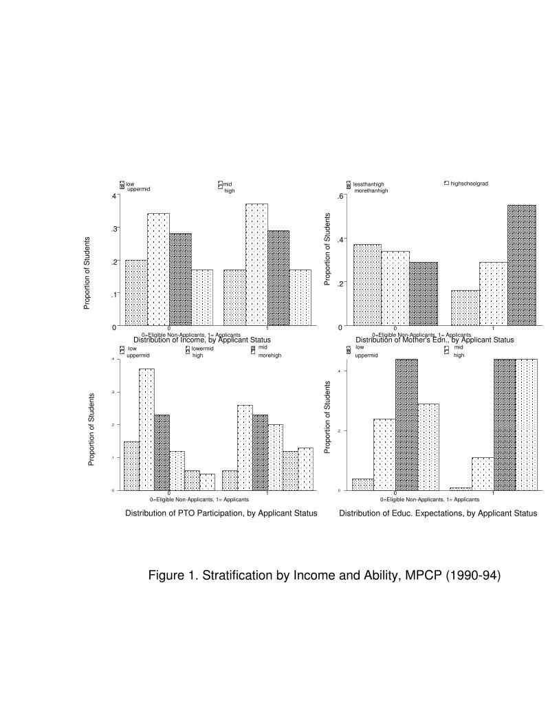
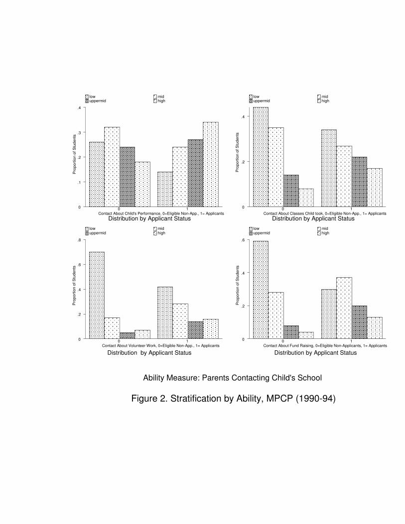
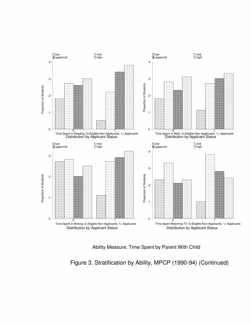
These patterns are mirrored in the graphical analysis (figures 1 and 2). While there is not much
difference between the income distribution of the applicants and non-applicants, the distribution of the
different ability measures are very different between these two groups. For each of the ability measures,
the proportions of choice households in the upper categories are much higher than the corresponding
non-applicant proportions while the proportions of applicants in the lower categories are much smaller.
This again supports stratification by ability.
I now investigate whether the pattern that arises from the bivariate comparisons and the income-
ability distribution figures is confirmed in a multivariate logistic regression framework. Using data
from MPCP applicants for 1990-94 and eligible non-applicants from the MPS, table 5 reports the
18 The only difference is that in 1994 the applicant households had economically and statistically higher income than
the non-applicants.
16
results from four alternative logit specifications. Columns (1)-(4) pool all the years together, while
(5)-(9) do a year-by-year analysis. The dependent variable here is a dummy variable “apply” that
takes on a value of one for choice applicants and a value of zero for eligible non-applicants. Each of the
columns controls for race and sex of the student, columns (3), (4), (5)-(9) also control for an indicator
variable indicating whether mother is employed full-time. All columns of this table report odds-ratios
for easier interpretation, the corresponding logit coefficients are available on request. Odds ratio and
standard error of the odds ratio are given by eb and S.E(b)eb respectively, where b denotes the logit
coefficient. Statistical significance corresponds to the logit coefficients, because it is the coefficient that
is normally distributed, not the odds-ratio.19 The odds-ratio says by how much the odds of “apply”
increases as the explanatory variable is increased by one unit.
The first column includes household income and the most basic ability measure, mother’s educa-
tion. Column (2) includes a more elaborate set of ability measures. These include the number of times
the household contacted the child’s school in the previous year (“contact”), whether the parents par-
ticipated in parent-teacher activities (“PTO participation”), the time the parent spends with the child
in various activities (“child-time”) in a normal week. Column (3) includes educational expectations of
the parent for the child and for a dummy variable indicating whether the mother is employed full-time.
The results are very similar across the different specifications. Household income is never statistically
significant and its odds-ratio is always very close to one, indicating that income does not have much
effect on the probability of application. On the other hand, all the ability measures are statistically
significant (except child-time), with odds-ratios exceeding one by large margins. Consider the logistic
regression in column (3). Although child-time is not significant, with the odds-ratio exactly equaling
19 Odds-ratio gives the ratio of odds of a one unit change in the explanatory variable and always takes the value eb,
where b denotes the logit coefficient, irrespective of the point of measurement. If p denotes probability, then odds at x
is given byp(x)
1−p(x), odds at (x + 1) by
p(x+1)1−p(x+1)
and the odds-ratio at x byp(x+1)
1−p(x+1)p(x)
1−p(x)
. Using the logistic distribution, it
can be easily seen that the odds ratio equals eb, where b is the coefficient.
17
unity, the other three ability measures are highly significant. A unit increase in mother’s education
increases the odds of application by 67%. A unit increase in the variables contact, PTO participation
and child-time increases the odds of application by 7%, 12% and 62% respectively.
Using the specification corresponding to column (3), column (3′) displays the impact on probability
of application if each of the categorical income and ability measures are changed from their minimum
to maximum values, while holding every other variable constant at its mean. Having a mother with a
college degree rather than one who dropped out of high school increases the probability of application
by 0.21. Having a household income of above $20,000 rather than a household income of below $5,000
increases the probability of application by 0.04, however note that income is not statistically significant.
Moving from the lowest category of the contact variable (parents never contacted the school) to the
highest category (parents contacted school 35 or more times in the course of the previous year) increases
the probability of application by 0.31. Students with parents who participated in all 5 parent-teacher
activities considered have a 0.12 higher probability of applying compared to students whose parents
never participated in any such activity. Parents who expect their students to go to graduate school
have a 0.26 higher probability of sending their child to a choice school than parents who expect their
child to just finish some high school. Spending time with the child, on the other hand, do not seem
to have a major effect on the probability of application, which is perhaps not what one would have
expected. Column (4) reports odds ratios from a logit regression that instead of using the previous
formulation of mother’s education and household income, includes dummies for various categories of
mother’s education and household income. The results are very similar to those obtained above.
Since considering all the five years together may camouflage some distinctive patterns that may be
present in one or more years, I next do a year-by-year analysis. Household income is never statistically
significant except in 1994 when the odds ratio equals 1.63. In each of the years, mother’s education
is highly significant, with the odds-ratios ranging from 1.75 in 1992 to 2.58 in 1994. The results for
18
contact, PTO participation, child-time and educational expectations are also similar to those obtained
from the earlier analysis.
Since the regressions above have multiple measures of ability, a potential concern here is muti-
collinearity. Using several methods, I find that multicollinearity is not likely to be a problem. First,
the correlation between the different variables never exceed 0.4 and almost always lie between -0.1
and 0.2. Second, the estimates are very robust to dropping of variables. Finally, the variance inflation
factor corresponding to the different coefficients never exceed 1.8. A rule of thumb often used is that
a variance inflation factor above 10 indicates multicollinearity.
To rule out the effect of any school specific factors, I next run logistic regressions that control
for school dummies. These regressions compare choice applicants to eligible non-applicants within
the same school. Columns (1) and (2) of table 5 pool all the years together while columns (3)-(7)
report results for individual years. All regressions control for race and sex of the student. Column
(1) includes mother’s education and household income as regressors, while column (2) includes a more
elaborate set of ability measures. The regressions for the individual years do not include the wider set
of ability measures since this leads to a considerable fall in sample size, (although the results remain
similar). Once again, table 5 shows that an increase in each of the ability measures (except child-time)
increases the probability of application, in fact the effect for mother’s education is now even stronger
than before. The pattern in income is very similar to that obtained earlier.
Table 6 looks at the effect of prior reading and math scores of students on the probability of appli-
cation. These logistic regressions also include mother’s education, income, sex and other demographic
variables. Since the prior scores pertain to different years, schools and grades, column (2) includes
year dummies, column (3) year and school dummies and column (4) year, school and grade dummies.
The patterns for mother’s education and income are very similar to earlier, although household in-
come is no longer significant in 1994. Prior reading score is never statistically significant. Although
19
prior math score is initially significant, it no longer remains significant after inclusion of year, school
dummies (column 3) and year, school, grade dummies (column 4). Moreover, the odds ratios for both
prior reading and prior math scores are very close to one. This indicates that not only statistically,
but economically also, an increase in prior scores has no effect on the probability of application. Prior
scores are often looked upon as ability measures in the literature. However, it should be noted here
that the above pattern does not suggest an absence of sorting by ability. While interpreting these
results, it should be kept in mind that many students do not have data on prior scores (for example,
just the inclusion of prior reading and math scores leads to a fall in sample size from 1638 (table 4,
column 1) to 765 (table 6, column 1), and this smaller sample may not be a random sample of the
applicants and eligible non-applicants.
The findings obtained in the empirical part of the paper can be summarized as follows. There
is strong and robust evidence in favor of stratification by ability. Not only is it manifest in simple
bivariate and graphical analyzes, but is also supported in a logistic framework. This pattern is robust
to inclusion of school dummies and holds for a variety of ability measures such as mother’s education,
contact, PTO participation and educational expectations. There is not much evidence in favor of
stratification by income. It is statistically significant only in 1994, even that effect no longer exists
after inclusion of year-of-test, school, grade dummies and prior scores. (However, as discussed above,
the regressions in table 6 should be interpreted with caution.) Moreover, the odds ratios for income
are never very far from one (except 1994), which further provides evidence that income is not a
major factor in the application decision. Thus the empirical findings strongly support the predictions
obtained from theory.
20
7 Conclusions
This paper analyzes the impact of voucher design on student sorting and more specifically investigates
whether random private school selection and the absence of topping up of vouchers can eliminate stu-
dent sorting. Much of the existing literature investigates the issue of sorting where private schools can
choose their students. However, in the publicly funded voucher experiments in the U.S.—Milwaukee,
Cleveland and Florida—the private schools are not permitted, by law, to discriminate between stu-
dents. This study addresses the issue of sorting in such circumstances, where the supply side force to
sorting (private school screening) is absent.
The focus of this paper is the Milwaukee voucher program which is characterized by both random
private school selection and the absence of topping up of vouchers. In the context of an equilibrium
model of household behavior, the paper argues that random private school selection alone cannot
preclude sorting by income and ability. However, random private school selection coupled with the
absence of topping up can obviate sorting by income, but not sorting by ability.
Implementing a logit estimation strategy and using multiple measures of ability, the paper then
shows that the testable predictions are validated empirically. There is robust evidence in favor of
stratification by ability but no consistent evidence of sorting by income. These results are robust to
alternative specifications and various measures of ability. To conclude, the paper makes an important
contribution to the literature on sorting—it points out, both theoretically and empirically, that random
private school selection along with the absence of topping up of vouchers can preclude sorting by
income. This finding has important policy implications.
Appendix A: Proofs of Results
Proof of Proposition 1. Before the imposition of vouchers, a public school household that is
indifferent to switching to a private school satisfies the following equality:
21
h(y − tQ∗) − c1 + αu(Q∗) = h(y) + αu(q). For each income level and given other parameters, there is
a unique α0 that solves this equation:
α0 =h(y) − h(y − tQ∗) + c1
u(Q∗) − u(q)A.1
After imposition of vouchers, a household that is indifferent between public and private options,
satisfies h(y + v − tQ∗) − c1 + αu(Q∗) = h(y) + αu(q) ⇒ αu(Q) − c1 = αu(q), since vouchers are not
allowed to be topped up. Note that since private school quality is not costly here, Q∗ = Q, where Q
is the highest private school quality. Since D = α[u(Q)− u(q)]− c1 is independent of income, there is
no sorting by income. Given other parameters, a unique ability level α1 solves this equation:
α1 =c1
u(Q) − u(q)< α0 A.2
α1 is less than α0 as the numerator of A.2 is smaller and the denominator larger than that in A.1.
Thus vouchers increase sorting by ability even when vouchers fully pay for private school tuition.
Proof of corollary 1. Sorting by ability: Before the imposition of vouchers, a public school
household that is indifferent to switching to a private school satisfies the following equality:
h(y − tQ∗− c2) − c1 + αu(Q∗) = h(y) + αu(q). For each income level and given other parameters, α2
solves this equation where α2 is given by:
α2 =h(y) − h(y − tQ∗
− c2) + c1
u(Q∗) − u(q)A.3
After imposition of vouchers, a household that is indifferent between public and private options,
satisfies h(y − c2) − c1 + αu(Q∗) = h(y) + αu(q). Given other parameters, a unique ability level α3
solves this equation:
α3 =h(y) − h(y − c2) + c1
u(Q) − u(q)< α2 A.4
α3 is less than α2 as the numerator of A.4 is smaller and the denominator larger than that in A.3.
Thus vouchers increase sorting by ability.
22
Sorting by income: Before the imposition of vouchers, for each ability level and given other
parameters, there exists a unique income level y0 that satisfies the following
h(y − tQ∗− c2) − c1 + αu(Q∗) = h(y) + αu(q) A.5
After the imposition of vouchers, for each ability level and given other parameters, there exists a
unique income level y1 that solves the equation:
h(y − c2) − c1 + αu(Q) = h(y) + αu(q) A.6
Note the left hand sides of A.5 and A.6 are identical. Since Q > Q∗ and (y − c2) > (y − tQ∗− c2), it
follows that y1 < y0. This implies that vouchers increase sorting by income.
References
Campbell, David E., Martin R. West and Paul E. Peterson (2005), “Participation in a
National, Means-tested School Voucher Program,” Journal of Policy Analysis and Management,
24(3).
Epple, Dennis and Richard Romano (1998), “Competition between Private and Public Schools,
Vouchers and Peer Group Effects,” American Economic Review 62(1), 33-62.
Epple, Dennis and Richard Romano (2002), “Educational Vouchers and Cream Skimming”
NBER Working Paper # 9354.
Epple, Dennis, David Figlio and Richard Romano (2004), “Competition between Private and
Public Schools: testing Stratification and Pricing Predictions,” Journal of Public Economics 88 (7-8),
1215-1245.
Howell, William G., Paul E. Peterson, with Patrick J.Wolf and David E. Campbell
(2002), The education gap: Vouchers and urban schools. Washington, DC: Brookings Institution
Press.
23
Howell, William G (2004), “Dynamic selection effects in a means-tested, urban school voucher
program,” Journal of Policy Analysis and Management, 23, 225-50.
Hoxby, Caroline (2003), “School Choice and School Competition: Evidence from the United
States”, Swedish Economic Policy Review.
Hsieh Chang-Tai and Miguel Urquiola (2003), “ When Schools Compete, how do they
Compete? An assessment of Chile’s nationwide School Voucher Program,” NBER Working Paper
#10008.
Levin, Henry M. (1998) “Educational vouchers: Effectiveness, choice, and costs”, Journal of
Policy Analysis and Management 17(3), 373-392.
Peterson, Paul E., William G. Howell and Jay P. Greene (1999), “Evaluation of the
Cleveland Voucher Program after Two Years,” Harvard University, Program on Education Policy
and Governance, PEPG # 99-02.
Witte, John F. (2000), “The Market Approach to Education: An analysis of America’s First
Voucher Program,” Princeton University Press, Princeton.
Witte, John F., and Christopher A. Thorn (1996), “Who Chooses? Voucher and Interdistrict
Choice Programs in Milwaukee,” American Journal of Education 104, 186-217.
Witte, John F., and Christopher A. Thorn (1995), The Milwaukee Parental Choice Program,
1990/1991-1994/1995 [computer file]. Madison, WI: John F. Witte and Christopher A. Thorn
[producers], Data and Program Library Service [distributor].
(http://dpls.dacc.wisc.edu/choice/choice index.html)
24
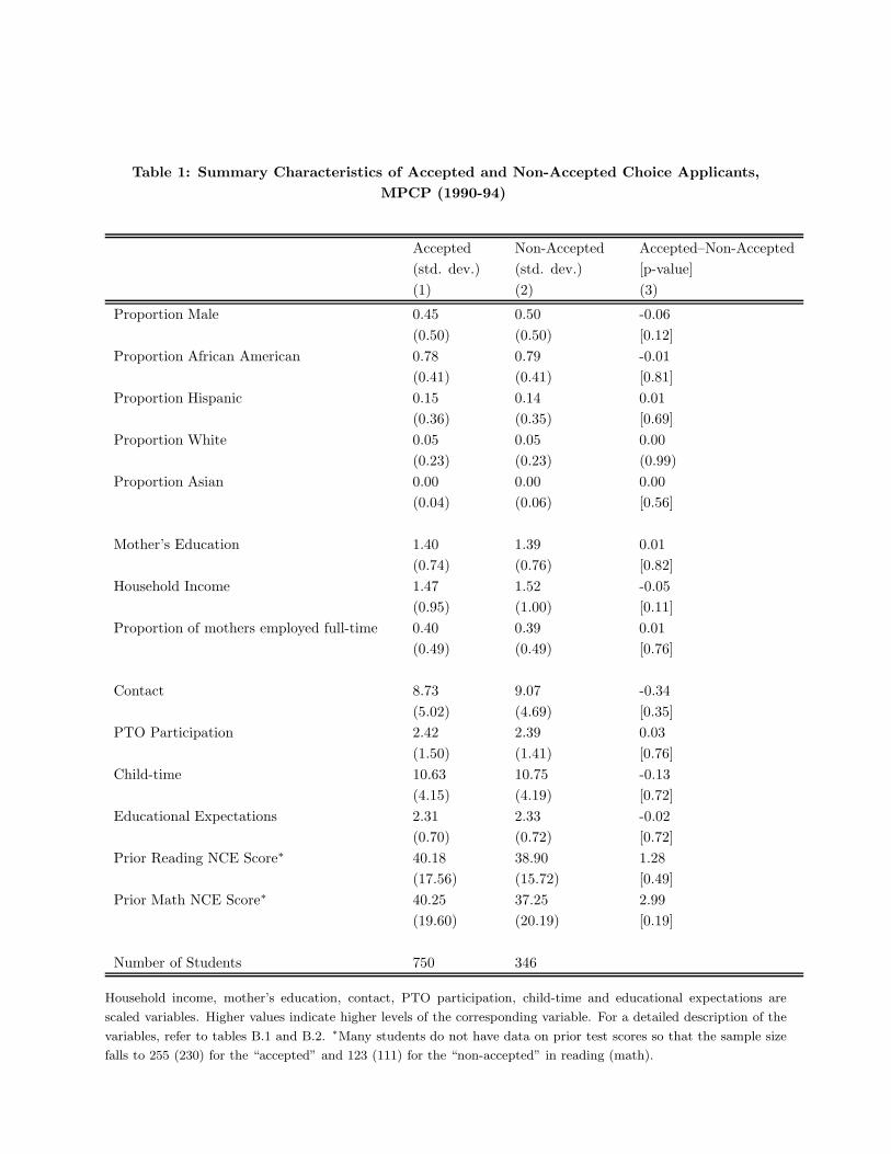
Table 1: Summary Characteristics of Accepted and Non-Accepted Choice Applicants,
MPCP (1990-94)
Accepted Non-Accepted Accepted–Non-Accepted
(std. dev.) (std. dev.) [p-value]
(1) (2) (3)
Proportion Male 0.45 0.50 -0.06
(0.50) (0.50) [0.12]
Proportion African American 0.78 0.79 -0.01
(0.41) (0.41) [0.81]
Proportion Hispanic 0.15 0.14 0.01
(0.36) (0.35) [0.69]
Proportion White 0.05 0.05 0.00
(0.23) (0.23) (0.99)
Proportion Asian 0.00 0.00 0.00
(0.04) (0.06) [0.56]
Mother’s Education 1.40 1.39 0.01
(0.74) (0.76) [0.82]
Household Income 1.47 1.52 -0.05
(0.95) (1.00) [0.11]
Proportion of mothers employed full-time 0.40 0.39 0.01
(0.49) (0.49) [0.76]
Contact 8.73 9.07 -0.34
(5.02) (4.69) [0.35]
PTO Participation 2.42 2.39 0.03
(1.50) (1.41) [0.76]
Child-time 10.63 10.75 -0.13
(4.15) (4.19) [0.72]
Educational Expectations 2.31 2.33 -0.02
(0.70) (0.72) [0.72]
Prior Reading NCE Score∗ 40.18 38.90 1.28
(17.56) (15.72) [0.49]
Prior Math NCE Score∗ 40.25 37.25 2.99
(19.60) (20.19) [0.19]
Number of Students 750 346
Household income, mother’s education, contact, PTO participation, child-time and educational expectations are
scaled variables. Higher values indicate higher levels of the corresponding variable. For a detailed description of the
variables, refer to tables B.1 and B.2. ∗Many students do not have data on prior test scores so that the sample size
falls to 255 (230) for the “accepted” and 123 (111) for the “non-accepted” in reading (math).
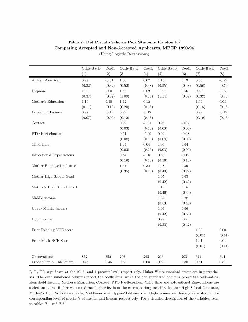
Table 2: Did Private Schools Pick Students Randomly?
Comparing Accepted and Non-Accepted Applicants, MPCP 1990-94
(Using Logistic Regressions)
Odds-Ratio Coeff. Odds-Ratio Coeff. Odds-Ratio Coeff. Odds-Ratio Coeff.
(1) (2) (3) (4) (5) (6) (7) (8)
African American 0.99 -0.01 1.08 0.07 1.13 0.13 0.80 -0.22
(0.32) (0.32) (0.52) (0.48) (0.55) (0.48) (0.56) (0.70)
Hispanic 1.00 0.00 1.86 0.62 1.93 0.66 0.43 -0.85
(0.37) (0.37) (1.09) (0.58) (1.14) (0.59) (0.32) (0.75)
Mother’s Education 1.10 0.10 1.12 0.12 1.09 0.08
(0.11) (0.10) (0.20) (0.18) (0.18) (0.16)
Household Income 0.87 -0.13 0.89 -0.12 0.82 -0.19
(0.07) (0.09) (0.12) (0.13) (0.10) (0.13)
Contact 0.99 -0.01 0.98 -0.02
(0.03) (0.03) (0.03) (0.03)
PTO Participation 0.91 -0.09 0.92 -0.08
(0.08) (0.09) (0.08) (0.09)
Child-time 1.04 0.04 1.04 0.04
(0.03) (0.03) (0.03) (0.03)
Educational Expectations 0.84 -0.18 0.83 -0.19
(0.16) (0.19) (0.16) (0.19)
Mother Employed full-time 1.37 0.32 1.48 0.39
(0.35) (0.25) (0.40) (0.27)
Mother High School Grad 1.05 0.05
(0.42) (0.40)
Mother> High School Grad 1.16 0.15
(0.46) (0.39)
Middle income 1.32 0.28
(0.53) (0.40)
Upper-Middle income 1.06 0.06
(0.42) (0.39)
High income 0.79 -0.23
(0.33) (0.42)
Prior Reading NCE score 1.00 0.00
(0.01) (0.01)
Prior Math NCE Score 1.01 0.01
(0.01) (0.01)
Observations 852 852 293 293 293 293 314 314
Probability > Chi-Square 0.45 0.45 0.68 0.68 0.80 0.80 0.51 0.51
∗, ∗∗, ∗∗∗: significant at the 10, 5, and 1 percent level, respectively. Huber-White standard errors are in parenthe-
ses. The even numbered columns report the coefficients, while the odd numbered columns report the odds-ratios.
Household Income, Mother’s Education, Contact, PTO Participation, Child-time and Educational Expectations are
scaled variables. Higher values indicate higher levels of the corresponding variable. Mother High School Graduate,
Mother> High School Graduate, Middle-income, Upper-Middleincome, High-income are dummy variables for the
corresponding level of mother’s education and income respectively. For a detailed description of the variables, refer
to tables B.1 and B.2.
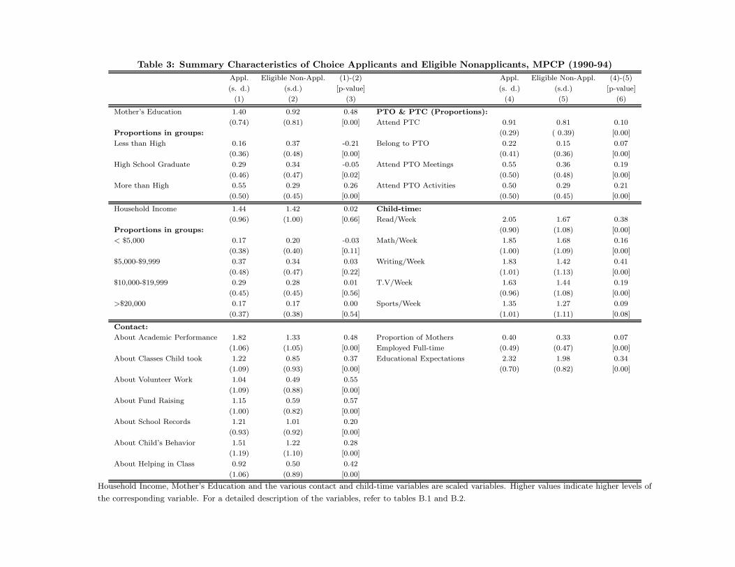
Table 3: Summary Characteristics of Choice Applicants and Eligible Nonapplicants, MPCP (1990-94)
Appl. Eligible Non-Appl. (1)-(2) Appl. Eligible Non-Appl. (4)-(5)
(s. d.) (s.d.) [p-value] (s. d.) (s.d.) [p-value]
(1) (2) (3) (4) (5) (6)
Mother’s Education 1.40 0.92 0.48 PTO & PTC (Proportions):
(0.74) (0.81) [0.00] Attend PTC 0.91 0.81 0.10
Proportions in groups: (0.29) ( 0.39) [0.00]
Less than High 0.16 0.37 -0.21 Belong to PTO 0.22 0.15 0.07
(0.36) (0.48) [0.00] (0.41) (0.36) [0.00]
High School Graduate 0.29 0.34 -0.05 Attend PTO Meetings 0.55 0.36 0.19
(0.46) (0.47) [0.02] (0.50) (0.48) [0.00]
More than High 0.55 0.29 0.26 Attend PTO Activities 0.50 0.29 0.21
(0.50) (0.45) [0.00] (0.50) (0.45) [0.00]
Household Income 1.44 1.42 0.02 Child-time:
(0.96) (1.00) [0.66] Read/Week 2.05 1.67 0.38
Proportions in groups: (0.90) (1.08) [0.00]
< $5,000 0.17 0.20 -0.03 Math/Week 1.85 1.68 0.16
(0.38) (0.40) [0.11] (1.00) (1.09) [0.00]
$5,000-$9,999 0.37 0.34 0.03 Writing/Week 1.83 1.42 0.41
(0.48) (0.47) [0.22] (1.01) (1.13) [0.00]
$10,000-$19,999 0.29 0.28 0.01 T.V/Week 1.63 1.44 0.19
(0.45) (0.45) [0.56] (0.96) (1.08) [0.00]
>$20,000 0.17 0.17 0.00 Sports/Week 1.35 1.27 0.09
(0.37) (0.38) [0.54] (1.01) (1.11) [0.08]
Contact:
About Academic Performance 1.82 1.33 0.48 Proportion of Mothers 0.40 0.33 0.07
(1.06) (1.05) [0.00] Employed Full-time (0.49) (0.47) [0.00]
About Classes Child took 1.22 0.85 0.37 Educational Expectations 2.32 1.98 0.34
(1.09) (0.93) [0.00] (0.70) (0.82) [0.00]
About Volunteer Work 1.04 0.49 0.55
(1.09) (0.88) [0.00]
About Fund Raising 1.15 0.59 0.57
(1.00) (0.82) [0.00]
About School Records 1.21 1.01 0.20
(0.93) (0.92) [0.00]
About Child’s Behavior 1.51 1.22 0.28
(1.19) (1.10) [0.00]
About Helping in Class 0.92 0.50 0.42
(1.06) (0.89) [0.00]
Household Income, Mother’s Education and the various contact and child-time variables are scaled variables. Higher values indicate higher levels of
the corresponding variable. For a detailed description of the variables, refer to tables B.1 and B.2.
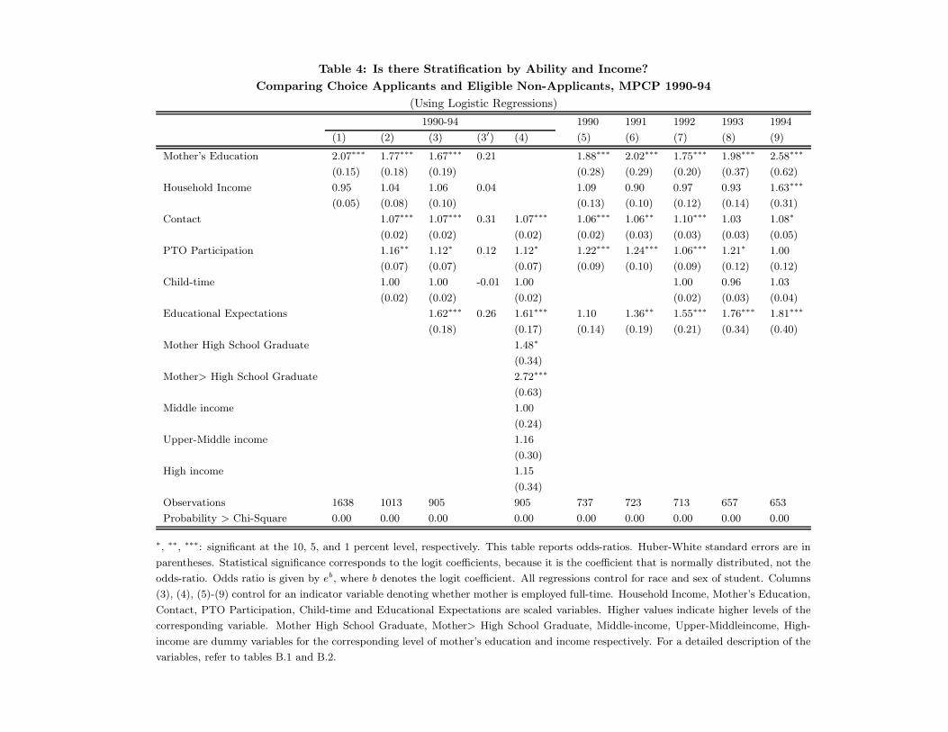
Table 4: Is there Stratification by Ability and Income?
Comparing Choice Applicants and Eligible Non-Applicants, MPCP 1990-94
(Using Logistic Regressions)
1990-94 1990 1991 1992 1993 1994
(1) (2) (3) (3′) (4) (5) (6) (7) (8) (9)
Mother’s Education 2.07∗∗∗ 1.77∗∗∗ 1.67∗∗∗ 0.21 1.88∗∗∗ 2.02∗∗∗ 1.75∗∗∗ 1.98∗∗∗ 2.58∗∗∗
(0.15) (0.18) (0.19) (0.28) (0.29) (0.20) (0.37) (0.62)
Household Income 0.95 1.04 1.06 0.04 1.09 0.90 0.97 0.93 1.63∗∗∗
(0.05) (0.08) (0.10) (0.13) (0.10) (0.12) (0.14) (0.31)
Contact 1.07∗∗∗ 1.07∗∗∗ 0.31 1.07∗∗∗ 1.06∗∗∗ 1.06∗∗ 1.10∗∗∗ 1.03 1.08∗
(0.02) (0.02) (0.02) (0.02) (0.03) (0.03) (0.03) (0.05)
PTO Participation 1.16∗∗ 1.12∗ 0.12 1.12∗ 1.22∗∗∗ 1.24∗∗∗ 1.06∗∗∗ 1.21∗ 1.00
(0.07) (0.07) (0.07) (0.09) (0.10) (0.09) (0.12) (0.12)
Child-time 1.00 1.00 -0.01 1.00 1.00 0.96 1.03
(0.02) (0.02) (0.02) (0.02) (0.03) (0.04)
Educational Expectations 1.62∗∗∗ 0.26 1.61∗∗∗ 1.10 1.36∗∗ 1.55∗∗∗ 1.76∗∗∗ 1.81∗∗∗
(0.18) (0.17) (0.14) (0.19) (0.21) (0.34) (0.40)
Mother High School Graduate 1.48∗
(0.34)
Mother> High School Graduate 2.72∗∗∗
(0.63)
Middle income 1.00
(0.24)
Upper-Middle income 1.16
(0.30)
High income 1.15
(0.34)
Observations 1638 1013 905 905 737 723 713 657 653
Probability > Chi-Square 0.00 0.00 0.00 0.00 0.00 0.00 0.00 0.00 0.00
∗, ∗∗, ∗∗∗: significant at the 10, 5, and 1 percent level, respectively. This table reports odds-ratios. Huber-White standard errors are in
parentheses. Statistical significance corresponds to the logit coefficients, because it is the coefficient that is normally distributed, not the
odds-ratio. Odds ratio is given by eb, where b denotes the logit coefficient. All regressions control for race and sex of student. Columns
(3), (4), (5)-(9) control for an indicator variable denoting whether mother is employed full-time. Household Income, Mother’s Education,
Contact, PTO Participation, Child-time and Educational Expectations are scaled variables. Higher values indicate higher levels of the
corresponding variable. Mother High School Graduate, Mother> High School Graduate, Middle-income, Upper-Middleincome, High-
income are dummy variables for the corresponding level of mother’s education and income respectively. For a detailed description of the
variables, refer to tables B.1 and B.2.
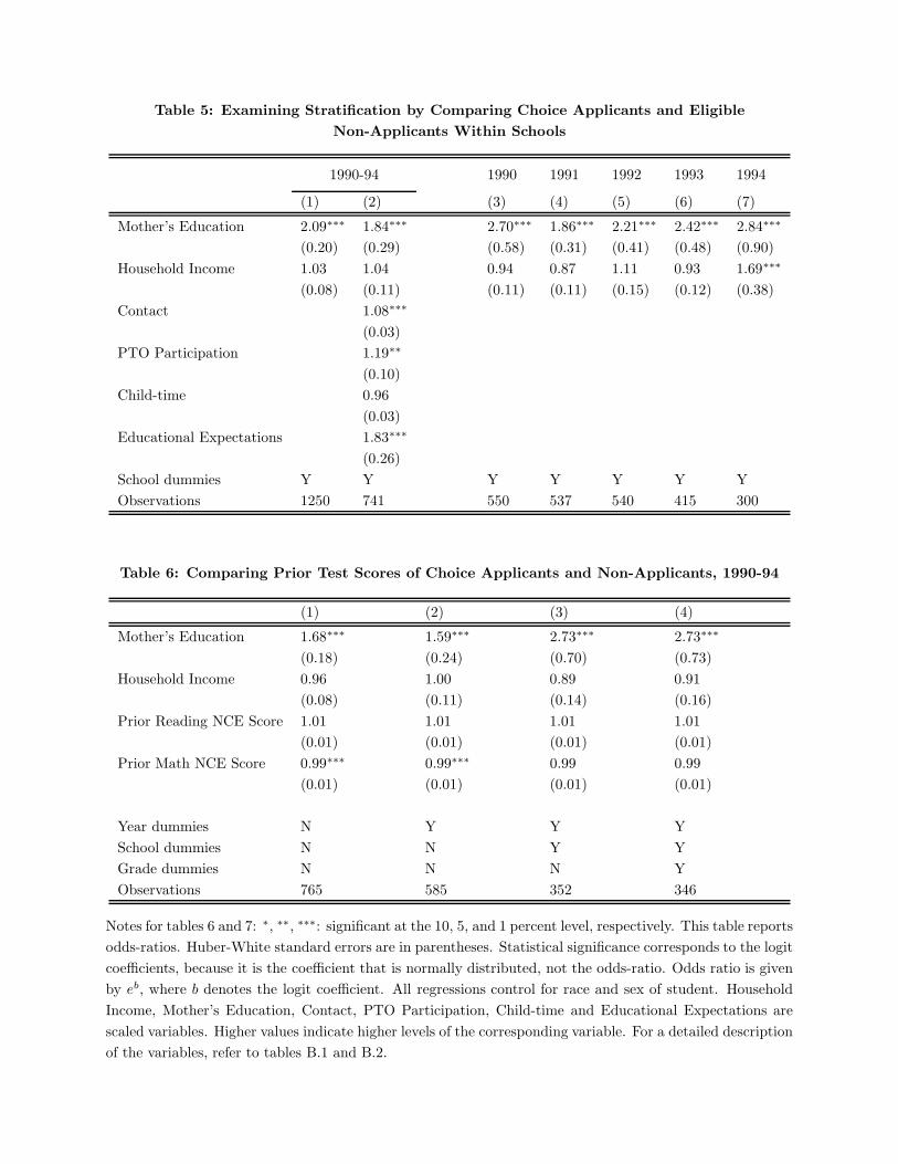
Table 5: Examining Stratification by Comparing Choice Applicants and Eligible
Non-Applicants Within Schools
1990-94 1990 1991 1992 1993 1994
(1) (2) (3) (4) (5) (6) (7)
Mother’s Education 2.09∗∗∗ 1.84∗∗∗ 2.70∗∗∗ 1.86∗∗∗ 2.21∗∗∗ 2.42∗∗∗ 2.84∗∗∗
(0.20) (0.29) (0.58) (0.31) (0.41) (0.48) (0.90)
Household Income 1.03 1.04 0.94 0.87 1.11 0.93 1.69∗∗∗
(0.08) (0.11) (0.11) (0.11) (0.15) (0.12) (0.38)
Contact 1.08∗∗∗
(0.03)
PTO Participation 1.19∗∗
(0.10)
Child-time 0.96
(0.03)
Educational Expectations 1.83∗∗∗
(0.26)
School dummies Y Y Y Y Y Y Y
Observations 1250 741 550 537 540 415 300
Table 6: Comparing Prior Test Scores of Choice Applicants and Non-Applicants, 1990-94
(1) (2) (3) (4)
Mother’s Education 1.68∗∗∗ 1.59∗∗∗ 2.73∗∗∗ 2.73∗∗∗
(0.18) (0.24) (0.70) (0.73)
Household Income 0.96 1.00 0.89 0.91
(0.08) (0.11) (0.14) (0.16)
Prior Reading NCE Score 1.01 1.01 1.01 1.01
(0.01) (0.01) (0.01) (0.01)
Prior Math NCE Score 0.99∗∗∗ 0.99∗∗∗ 0.99 0.99
(0.01) (0.01) (0.01) (0.01)
Year dummies N Y Y Y
School dummies N N Y Y
Grade dummies N N N Y
Observations 765 585 352 346
Notes for tables 6 and 7: ∗, ∗∗, ∗∗∗: significant at the 10, 5, and 1 percent level, respectively. This table reports
odds-ratios. Huber-White standard errors are in parentheses. Statistical significance corresponds to the logit
coefficients, because it is the coefficient that is normally distributed, not the odds-ratio. Odds ratio is given
by eb, where b denotes the logit coefficient. All regressions control for race and sex of student. Household
Income, Mother’s Education, Contact, PTO Participation, Child-time and Educational Expectations are
scaled variables. Higher values indicate higher levels of the corresponding variable. For a detailed description
of the variables, refer to tables B.1 and B.2.
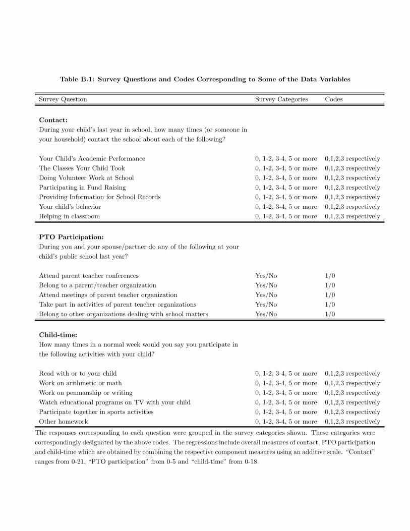
Table B.1: Survey Questions and Codes Corresponding to Some of the Data Variables
Survey Question Survey Categories Codes
Contact:
During your child’s last year in school, how many times (or someone in
your household) contact the school about each of the following?
Your Child’s Academic Performance 0, 1-2, 3-4, 5 or more 0,1,2,3 respectively
The Classes Your Child Took 0, 1-2, 3-4, 5 or more 0,1,2,3 respectively
Doing Volunteer Work at School 0, 1-2, 3-4, 5 or more 0,1,2,3 respectively
Participating in Fund Raising 0, 1-2, 3-4, 5 or more 0,1,2,3 respectively
Providing Information for School Records 0, 1-2, 3-4, 5 or more 0,1,2,3 respectively
Your child’s behavior 0, 1-2, 3-4, 5 or more 0,1,2,3 respectively
Helping in classroom 0, 1-2, 3-4, 5 or more 0,1,2,3 respectively
PTO Participation:
During you and your spouse/partner do any of the following at your
child’s public school last year?
Attend parent teacher conferences Yes/No 1/0
Belong to a parent/teacher organization Yes/No 1/0
Attend meetings of parent teacher organization Yes/No 1/0
Take part in activities of parent teacher organizations Yes/No 1/0
Belong to other organizations dealing with school matters Yes/No 1/0
Child-time:
How many times in a normal week would you say you participate in
the following activities with your child?
Read with or to your child 0, 1-2, 3-4, 5 or more 0,1,2,3 respectively
Work on arithmetic or math 0, 1-2, 3-4, 5 or more 0,1,2,3 respectively
Work on penmanship or writing 0, 1-2, 3-4, 5 or more 0,1,2,3 respectively
Watch educational programs on TV with your child 0, 1-2, 3-4, 5 or more 0,1,2,3 respectively
Participate together in sports activities 0, 1-2, 3-4, 5 or more 0,1,2,3 respectively
Other homework 0, 1-2, 3-4, 5 or more 0,1,2,3 respectively
The responses corresponding to each question were grouped in the survey categories shown. These categories were
correspondingly designated by the above codes. The regressions include overall measures of contact, PTO participation
and child-time which are obtained by combining the respective component measures using an additive scale. “Contact”
ranges from 0-21, “PTO participation” from 0-5 and “child-time” from 0-18.
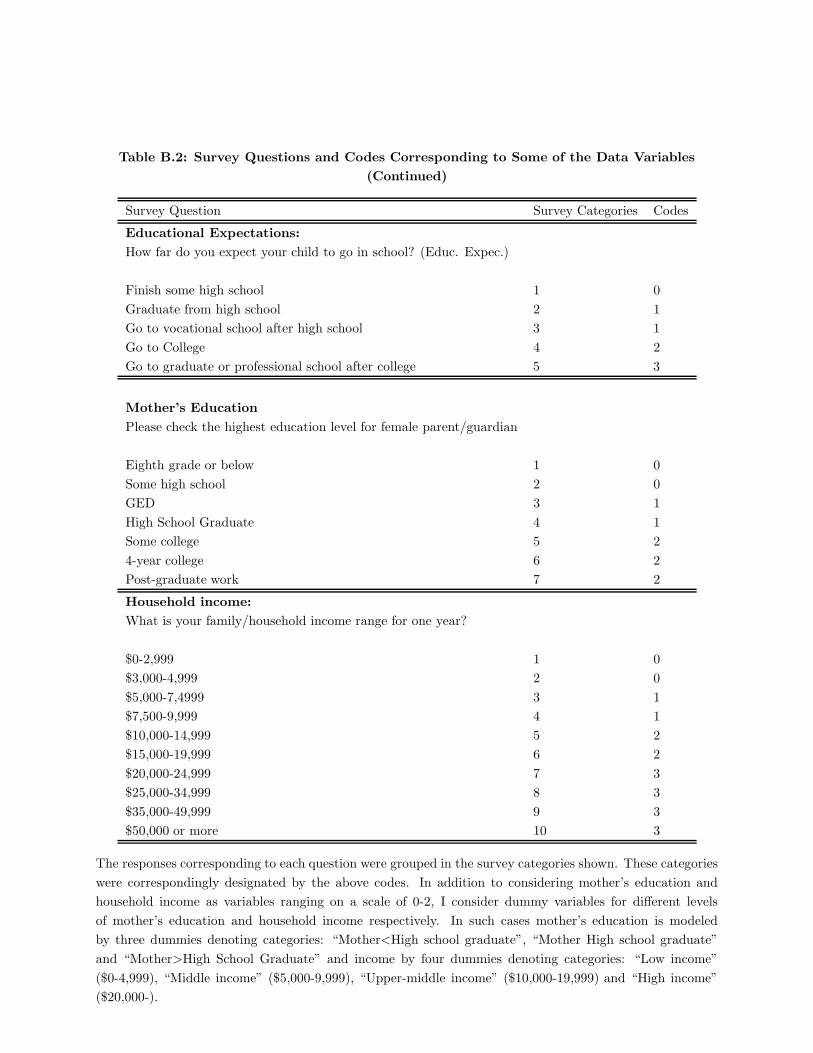
Table B.2: Survey Questions and Codes Corresponding to Some of the Data Variables
(Continued)
Survey Question Survey Categories Codes
Educational Expectations:
How far do you expect your child to go in school? (Educ. Expec.)
Finish some high school 1 0
Graduate from high school 2 1
Go to vocational school after high school 3 1
Go to College 4 2
Go to graduate or professional school after college 5 3
Mother’s Education
Please check the highest education level for female parent/guardian
Eighth grade or below 1 0
Some high school 2 0
GED 3 1
High School Graduate 4 1
Some college 5 2
4-year college 6 2
Post-graduate work 7 2
Household income:
What is your family/household income range for one year?
$0-2,999 1 0
$3,000-4,999 2 0
$5,000-7,4999 3 1
$7,500-9,999 4 1
$10,000-14,999 5 2
$15,000-19,999 6 2
$20,000-24,999 7 3
$25,000-34,999 8 3
$35,000-49,999 9 3
$50,000 or more 10 3
The responses corresponding to each question were grouped in the survey categories shown. These categories
were correspondingly designated by the above codes. In addition to considering mother’s education and
household income as variables ranging on a scale of 0-2, I consider dummy variables for different levels
of mother’s education and household income respectively. In such cases mother’s education is modeled
by three dummies denoting categories: “Mother<High school graduate”, “Mother High school graduate”
and “Mother>High School Graduate” and income by four dummies denoting categories: “Low income”
($0-4,999), “Middle income” ($5,000-9,999), “Upper-middle income” ($10,000-19,999) and “High income”
($20,000-).
Pro
port
ion o
f S
tudents
Distribution of Income, by Applicant Status 0=Eligible Non-Applicants, 1= Applicants
0
.1
.2
.3
.4 uppermid high
0 1 P
roport
ion o
f S
tudents
Distribution of Mother's Edn., by Applicant Status 0=Eligible Non-Applicants, 1= Applicants
0
.2
.4
.6
highschoolgrad
0 1
Pro
port
ion o
f S
tudents
Distribution of PTO Participation, by Applicant Status
0=Eligible Non-Applicants, 1= Applicants
0
.1
.2
.3
.4 low lowermid mid
uppermid high morehigh
0 1
Pro
port
ion o
f S
tudents
Distribution of Educ. Expectations, by Applicant Status
0=Eligible Non-Applicants, 1= Applicants
0
.2
.4
low mid
uppermid high
0 1
morethanhigh low mid lessthanhigh
Figure 1. Stratification by Income and Ability, MPCP (1990-94)
Ability Measure: Parents Contacting Child's School
Pro
po
rtio
n o
f S
tud
en
ts
Distribution by Applicant Status Contact About Child's Performance, 0=Eligible Non-App., 1= Applicants
0
.1
.2
.3
.4
low mid uppermid high
0 1
Pro
po
rtio
n o
f S
tud
en
ts
Distribution by Applicant Status Contact About Classes Child took, 0=Eligible Non-App., 1= Applicants
0
.2
.4
low mid uppermid high
0 1
Pro
po
rtio
n o
f S
tud
en
ts
Distribution by Applicant Status Contact About Volunteer Work, 0=Eligible Non-App., 1= Applicants
0
.2
.4
.6
.8
low mid uppermid high
0 1
Pro
po
rtio
n o
f S
tud
en
ts
Distribution by Applicant Status Contact About Fund Raising, 0=Eligible Non-Applicants, 1= Applicants
0
.2
.4
.6
low mid uppermid high
0 1
Figure 2. Stratification by Ability, MPCP (1990-94)
Ability Measure: Time Spent by Parent With Child
Pro
port
ion o
f S
tud
ents
Distribution by Applicant Status Time Spent in Reading, 0=Eligible Non-Applicants, 1= Applicants
0
.1
.2
.3
.4
low mid uppermid high
0 1
Pro
port
ion o
f S
tud
ents
Distribution by Applicant Status Time Spent in Math, 0=Eligible Non-Applicants, 1= Applicants
0
.1
.2
.3
.4
low mid uppermid high
0 1
Pro
port
ion o
f S
tud
ents
Distribution by Applicant Status Time Spent in Writing, 0=Eligible Non-Applicants, 1= Applicants
0
.1
.2
.3
low mid uppermid high
0 1
Pro
port
ion o
f S
tud
ents
Distribution by Applicant Status Time Spent Watching TV, 0=Eligible Non-Applicants, 1= Applicants
0
.1
.2
.3
.4
low mid uppermid high
0 1
Figure 3. Stratification by Ability, MPCP (1990-94) (Continued)