Working Paper 1906 Research Department https://doi.org/10.24149/wp1906

Working papers from the Federal Reserve Bank of Dallas are preliminary drafts circulated for professional comment. The views in this paper are those of the authors and do not necessarily reflect the views of the Federal Reserve Bank of Dallas or the Federal Reserve System. Any errors or omissions are the responsibility of the authors.

Do Monetary Policy Announcements Shift Household Expectations?

Daniel J. Lewis, Christos Makridis and Karel Mertens

Do Monetary Policy Announcements Shift Household Expectations?*

Daniel J. Lewis†, Christos Makridis‡ and Karel Mertens§

September 3, 2019

Abstract We use daily survey data from Gallup to assess whether households' beliefs about economic conditions are influenced by surprises in monetary policy announcements. We first provide more general evidence that public confidence in the state of the economy reacts to certain types of macroeconomic news very quickly. Next, we show that surprises to the Federal Funds target rate are among the news that have statistically significant and instantaneous effects on economic confidence. In contrast, surprises about forward guidance and asset purchases do not have similar effects on household beliefs, perhaps because they are less well understood. We document heterogeneity in the responsiveness of sentiment across demographics. JEL Codes: E30, E40, E50, E70 Keywords: Monetary policy shocks, central bank communication, information rigidities, consumer confidence, high frequency identification

*Christos Makridis thanks Gallup and their support team for academic partnership. The views in this paper are those of the authors and do not necessarily reflect the views of the Federal Reserve Banks of Dallas and New York or the Federal Reserve System. †Daniel J. Lewis, Federal Reserve Bank of New York. ‡Christos Makridis, MIT Sloan. §Contact: Karel Mertens, Federal Reserve Bank of Dallas, mertens.karel@gmail.com, + (214) 922-6000.

1 Introduction

In the early 1990s, the Federal Reserve began informing the public about its monetary policy

decisions immediately after policy meetings. In 2012, the FOMC publicly announced a two per-

cent inflation target as the most consistent with its price stability objective. FOMC members

nowadays routinely communicate their views on the economic outlook as well as on appropriate

future adjustments to monetary policy. Besides fostering accountability, the rationale for these

and other steps towards greater transparency is to facilitate the management of expectations

and increase the effectiveness of monetary policy. In theory, effective central bank communi-

cation makes policy decisions more predictable, anchors long run inflation expectations more

firmly, and creates additional policy options at the zero lower bound in the form of forward

guidance about the path of future policy rates (Blinder 2008).

In practice, the benefits of increased transparency depend importantly on whether central

bank communications indeed steer the beliefs of economic agents successfully, i.e. in the de-

sired direction and with relatively short delays. There is much evidence that monetary policy

announcements influence the expectations of professional forecasters and financial market par-

ticipants.1 Much less is known about how strongly central bank communications influence the

beliefs of the broader public, i.e. the households and firms that ultimately account for the bulk

of economic decisions that monetary policy seeks to influence.

In this paper, we present evidence that monetary policy announcements about the interest

rate target have a meaningful and immediate impact on household beliefs about macroeconomic

conditions. To measure monetary policy news, we follow the high frequency identification ap-

proach and use movements in asset prices on FOMC meeting days. Our baseline measures

of household beliefs are based on survey questions about national economic conditions from

the U.S. Daily Survey Poll conducted by Gallup between January 2008 and December 2017.

The answers are combined in daily diffusion indices that are very similar to existing monthly

consumer confidence indices constructed from the Michigan or Conference Board surveys. We

also verify our results using an alternative daily dataset produced by Rasmussen.

Importantly, the high frequency of the confidence measures allows us to estimate the im-

pact of monetary policy announcements on agents’ economic outlook on the days immediately

following the arrival of the monetary policy news. This permits the interpretation of the esti-

mated confidence effects as a reevaluation of beliefs by agents in light of new information about

monetary policy, and not as an indirect response to changes in subsequent macroeconomic data

releases or in agents’ own economic situation that may result from the economic consequences

of the monetary policy announcement. In addition, we can be more confident that the expecta-

tions effects are due to monetary policy announcements and not to other confounding factors.

1See for instance Lucca and Trebbi (2009), Campbell et al. (2012), Del Negro, Giannoni, and Patterson(2015), Altavilla and Giannone (2017), Nakamura and Steinsson (2018), and Cieslak and Schrimpf (2019).

2

In other words, the exclusion restriction required for event study analysis is more plausibly

justified in this daily data than in lower-frequency studies.

Our sample period – January 2008 to December 2017 – includes the use of both conventional

and unconventional policy instruments by the Federal Reserve. Based on financial market data

on FOMC days, Swanson (2017) shows that monetary policy announcements over this period

contain information that is consistent with the use of three distinct policy instruments: changes

in current policy rates, forward guidance about future policy rates, and large scale asset pur-

chases (LSAPs). The distinction between policy instruments is potentially important as the

unconventional tools deployed by the FOMC in the wake of the Global Financial Crisis (GFC)

may be less well understood by the general public and therefore affect perceptions of economic

conditions differently. Our baseline methodology follows Lewis (2019) and separately identifies

the impact on household economic confidence of monetary policy news about each of these

three policy instruments. We also confirm our findings using a range of other available high

frequency measures of monetary policy news.

Our first main empirical result is that news about current policy rates has instantaneous,

persistent and highly statistically significant effects on aggregate household beliefs about the

state of the national economy. A surprise tightening of 25 basis points leads to an immediate

deterioration in the daily economic confidence index equivalent to 1 to 2 points of the Michigan

Index of Consumer Sentiment. This means that in our sample households interpret a positive

target rate surprise on average as negative for the US economy. This finding indicates that the

transmission of target rate surprises to the real economy operates at least in part through a

direct and immediate effect on household confidence. We also analyze the heterogeneity of the

belief responses to monetary policy news across different age, income and education groups.

We find evidence that the responsiveness to the funds rate surprises is stronger among more

highly educated and younger respondents, and we relate this to evidence of relatively higher

rates of information updating for these groups.

Our second main result is that, while there is much evidence that forward guidance and

LSAPs affect longer term interest rates by influencing expectations in financial markets, we

find no systematic evidence for any immediate statistically significant effects of new informa-

tion about these policies on household beliefs.2 This finding suggests that these policies have

been less effective than conventional target rate changes to stimulate aggregate spending in

the aftermath of the GFC, at least in the short run. It is of course possible that growing

public familiarity and a more systematic implementation of forward guidance and LSAPs may

make these alternative policy tools more effective substitutes for target rate changes in future

experiences with the ZLB. Nevertheless, our results suggest that further improvements in com-

munication to the wider public may be warranted to increase the potency of non-interest rate

2For a recent overview of the evidence on the effects of unconventional policies on asset prices, see Eberly,Stock, and Wright (2019).

3

policies.

Our finding that economic confidence responds instantaneously to conventional monetary

policy news offers counter-evidence to a widespread view that central banks have limited in-

fluence over expectations held by the general public. An overview study by Binder (2017),

for example, expresses doubts that central bank communications are transmitted effectively to

households. Survey evidence points to low public informedness about monetary policy. On

the one hand, poor economic and financial literacy imply low demand for monetary policy

information as cognitive costs outweigh economic benefits.3 Intense competition for audience

attention, on the other hand, results in limited media coverage of central bank news.

More broadly, the available evidence on the formation of expectations suggests that in-

formational rigidities are very important. Carroll (2003), for instance, finds that consumers

only very occasionally pay attention to news reports. As a result, consumer expectations track

those of professional forecasters with very long delays (one year on average). Coibion and

Gorodnichenko (2015) show that the empirical relationships between survey forecast errors and

forecast revisions also imply large degrees of informational rigidities. Based on all of the evi-

dence for inattentiveness, Coibion et al. (2018) are skeptical that central bank communication

can successfully manipulate household’s inflation expectations, at least in a low inflation envi-

ronment and with existing communication strategies.

Given the broad acceptance in the literature of pervasive inattentiveness to monetary pol-

icy, our finding that unexpected target rate changes have immediate measurable effects on

consumer confidence is perhaps somewhat surprising. There are, however a number of impor-

tant differences between our analysis and the existing evidence for inattentiveness. For one,

the high frequency aspect of the Gallup data is much better suited than monthly or quarterly

survey data to isolate and interpret the drivers of household beliefs, and also avoids problems

of time aggregation. It allows us to show, for instance, that daily consumer confidence can

react strongly and swiftly to important news events, and responds significantly to some of the

major official macroeconomic data releases such as the jobs and GDP reports. These findings

add plausibility to our claim that households beliefs about the economy can also shift quickly

in response to monetary policy news.

Another key difference with earlier work is that we look at belief measures constructed

from categorical answers to questions about the state of the national economy. The existing

literature focuses predominantly on quantitative answers to questions about expected inflation

rates. Agents may be more attentive to information relevant for broader economic conditions

than to information relevant for inflation. Incorporating this information into broad categori-

cal responses may also be simpler and require less effort than translating this information into

3or as Blinder (2018) puts it: “most people are not obsessed about the central bank; ... they would ratherwatch puppies on YouTube.”

4

quantitative changes to inflation projections. We verify these conjectures by estimating the

degree of ‘information stickiness’ building on Carroll (2003). We find indeed that daily house-

hold confidence tracks information in financial markets much more quickly, with an estimated

average time between information updates of less than two weeks. Respondents with a college

degree update more frequently than respondents with lower education levels.

The remainder of the paper is organized as follows. Section 2 introduces describes the

Gallup data and its relation to alternative measures. Section 3 examines the response of

consumer sentiment to macroeconomic news, broadly defined. Section 4 analyzes the response

to monetary policy surprises. Section 5 concludes.

2 High Frequency Measures of Economic Confidence

Most of the results in this paper are based on daily survey information collected by Gallup.

Founded in 1935, Gallup is one of the world’s premier polling and analytics companies. In

2008 it began interviewing roughly 1,000 Americans by telephone on political, economic, and

well-being topics in their U.S. Daily Poll.4 From 2008 to the end of 2017, about half of the

respondents were asked two questions about the state of the national economy.5 The first

question asks the respondents’ view on the current state of economic conditions:

1. Rate economic conditions in the country today. (1) Excellent; (2) Good; (3) Only fair; or

(4) Poor?

The second question asks about the direction of economic conditions:

2. Do you think economic conditions in the country as a whole are getting (1) better or (2)

worse?

Note that both the “current state” and “direction” questions explicitly refer to national

economic conditions. While economic conditions is admittedly subject to interpretation, re-

spondents typically proxy for macroeconomic conditions using simple heuristics, such as the

unemployment rate or GDP growth rate. Other interview questions ask specifically about

respondents’ own economic or financial situation. Since our interest is in a measure of macroe-

conomic beliefs, we only use the questions about the national economic conditions.

Gallup combines the answers to the two questions above in an Economic Confidence Index

(ECI). This ECI index is computed by adding the percentage of respondents rating current

economic conditions ((“Excellent” + “Good”) minus “Poor”) to the percentage saying the

economy is (“Getting better” minus “Getting worse”) and then dividing that sum by 2. The

aggregation uses weighting adjustments to make the index representative of the US population.

4The online publication Understanding Gallup’s Economic Measures provides additional information.5The sample size is close to 1,000 between from Jan 2 to Jan 20 in 2008; it is close to 500 between Jan 21,

2008 and July 30 2017; and it varies in a range of around 300 to 700 between July 31 and December 31, 2017.

5

(a) Economic Confidence Index

01-0

1-08

01-0

1-09

01-0

1-10

01-0

1-11

01-0

1-12

01-0

1-13

01-0

1-14

01-0

1-15

01-0

1-16

01-0

1-17

01-0

1-18

01-0

1-19

40

50

60

70

80

90

100

110

Negative ECI Change PointPositive ECI Change PointGallup ECIMichigan Index

(b) Current State of Economic Conditions

01-0

1-08

01-0

1-09

01-0

1-10

01-0

1-11

01-0

1-12

01-0

1-13

01-0

1-14

01-0

1-15

01-0

1-16

01-0

1-17

01-0

1-18

01-0

1-19

40

50

60

70

80

90

100

110

120

Negative ECI Change PointPositive ECI Change PointGallup Current State Index

(c) Direction of Economic Conditions

01-0

1-08

01-0

1-09

01-0

1-10

01-0

1-11

01-0

1-12

01-0

1-13

01-0

1-14

01-0

1-15

01-0

1-16

01-0

1-17

01-0

1-18

01-0

1-19

20

40

60

80

100

120

Negative ECI Change PointPositive ECI Change PointGallup Direction Index

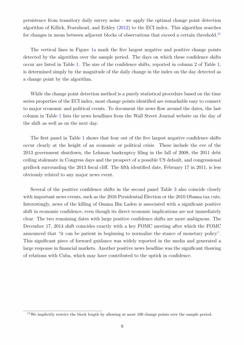
Figure 1: Daily Gallup Confidence Indices and the Michigan Sentiment Index.

Notes: Data from Gallup and University of Michigan. Shaded areas are NBER recessions. The daily Gallupindices cover January 2, 2008 through December 27, 2017 and each rescaled to have the same mean and varianceas the Michigan Sentiment Index over this period.

6

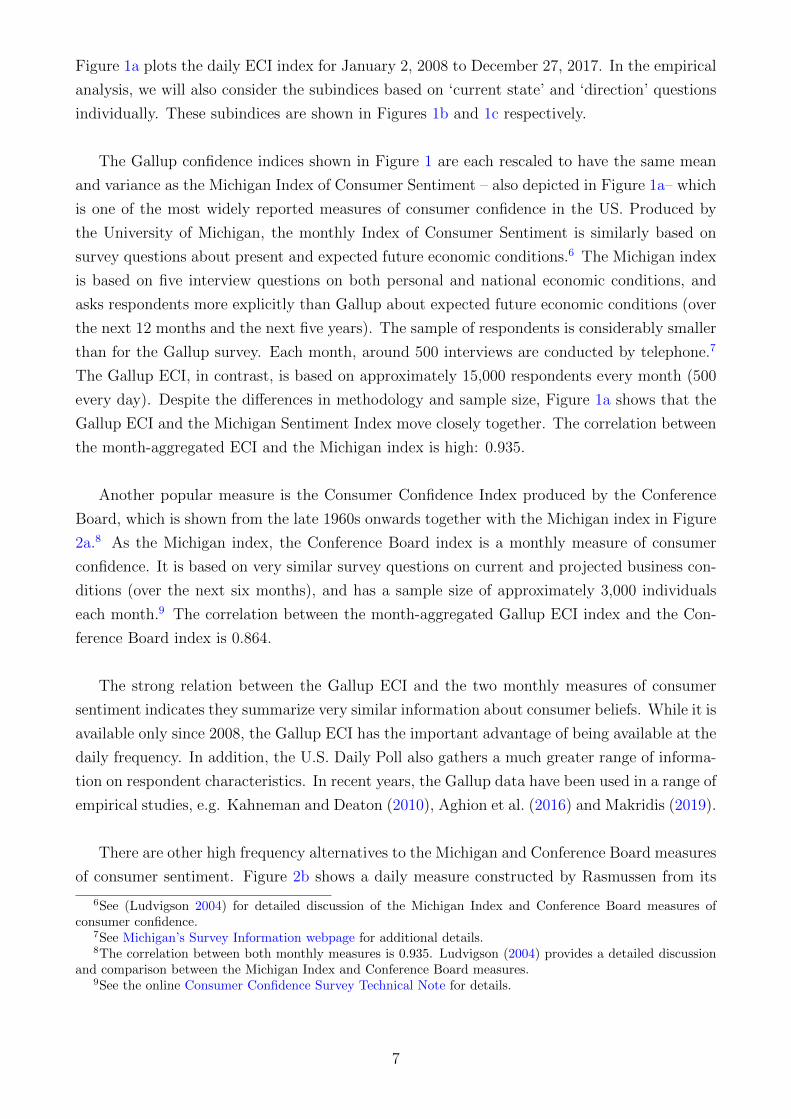
Figure 1a plots the daily ECI index for January 2, 2008 to December 27, 2017. In the empirical

analysis, we will also consider the subindices based on ‘current state’ and ‘direction’ questions

individually. These subindices are shown in Figures 1b and 1c respectively.

The Gallup confidence indices shown in Figure 1 are each rescaled to have the same mean

and variance as the Michigan Index of Consumer Sentiment – also depicted in Figure 1a– which

is one of the most widely reported measures of consumer confidence in the US. Produced by

the University of Michigan, the monthly Index of Consumer Sentiment is similarly based on

survey questions about present and expected future economic conditions.6 The Michigan index

is based on five interview questions on both personal and national economic conditions, and

asks respondents more explicitly than Gallup about expected future economic conditions (over

the next 12 months and the next five years). The sample of respondents is considerably smaller

than for the Gallup survey. Each month, around 500 interviews are conducted by telephone.7

The Gallup ECI, in contrast, is based on approximately 15,000 respondents every month (500

every day). Despite the differences in methodology and sample size, Figure 1a shows that the

Gallup ECI and the Michigan Sentiment Index move closely together. The correlation between

the month-aggregated ECI and the Michigan index is high: 0.935.

Another popular measure is the Consumer Confidence Index produced by the Conference

Board, which is shown from the late 1960s onwards together with the Michigan index in Figure

2a.8 As the Michigan index, the Conference Board index is a monthly measure of consumer

confidence. It is based on very similar survey questions on current and projected business con-

ditions (over the next six months), and has a sample size of approximately 3,000 individuals

each month.9 The correlation between the month-aggregated Gallup ECI index and the Con-

ference Board index is 0.864.

The strong relation between the Gallup ECI and the two monthly measures of consumer

sentiment indicates they summarize very similar information about consumer beliefs. While it is

available only since 2008, the Gallup ECI has the important advantage of being available at the

daily frequency. In addition, the U.S. Daily Poll also gathers a much greater range of informa-

tion on respondent characteristics. In recent years, the Gallup data have been used in a range of

empirical studies, e.g. Kahneman and Deaton (2010), Aghion et al. (2016) and Makridis (2019).

There are other high frequency alternatives to the Michigan and Conference Board measures

of consumer sentiment. Figure 2b shows a daily measure constructed by Rasmussen from its

6See (Ludvigson 2004) for detailed discussion of the Michigan Index and Conference Board measures ofconsumer confidence.

7See Michigan’s Survey Information webpage for additional details.8The correlation between both monthly measures is 0.935. Ludvigson (2004) provides a detailed discussion

and comparison between the Michigan Index and Conference Board measures.9See the online Consumer Confidence Survey Technical Note for details.

7

(a) Conference Board ConsumerConfidence Index

1960 1970 1980 1990 2000 201050

60

70

80

90

100

110

120

Conference Board Consumer ConfidenceMichigan Index of Consumer Sentiment

(b) Rasmussen ConsumerConfidence Index

2006 2008 2010 2012 2014 2016 201850

60

70

80

90

100

110

120

Rasmussen Consumer IndexMichigan Index of Consumer Sentiment

Figure 2: Alternative Measures of Economic Confidence

Notes: Source: Gallup, Rasmussen, University of Michigan, Conference Board. Shaded areas are NBER reces-sions.

our daily national surveys of American consumers.10 The index published by Rasmussen is

a 3-day moving average and is based on a smaller number of respondents than the Gallup

ECI. The correlation between the month-aggregated Rasmussen index and the Michigan and

Conference Board indices are 0.969 and 0.940 respectively. We will nevertheless verify our main

results using this alternative daily confidence measure. Finally, Langer research also produces

a weekly index, which is branded by Bloomberg as the Consumer Comfort index. This measure

is based on a much smaller sample (approximately 250 respondents weekly) and is reported in

a four-week rolling average. As it is therefore less suitable for our high frequency analysis, we

do not use the Bloomberg Comfort Index.

3 Do Daily Confidence Measures Respond to Macroeconomic News?

Before turning to the reaction of households beliefs to monetary policy news, we first provide

some broader evidence on the responsiveness of survey-based confidence measures to macroeco-

nomic news. Exploiting the daily frequency of the Gallup measures, we discuss in turn reactions

to major news events, to surprises in macroeconomic data releases, and to information in fi-

nancial markets and other daily economic indicators.

3.1 Confidence Shifts Following Major News Events

One feature of consumer confidence revealed by the daily frequency of the Gallup measures is

the presence of occasional large and sudden single day shifts, see Figure 1. To formally iden-

tify these sudden shifts in economic confidence – and distinguish genuine belief shifts of some

10See the Rasmussen Reports methodology webpage for additional information.

8

persistence from transitory daily survey noise – we apply the optimal change point detection

algorithm of Killick, Fearnhead, and Eckley (2012) to the ECI index. This algorithm searches

for changes in mean between adjacent blocks of observations that exceed a certain threshold.11

The vertical lines in Figure 1a mark the five largest negative and positive change points

detected by the algorithm over the sample period. The days on which these confidence shifts

occur are listed in Table 1. The size of the confidence shifts, reported in column 2 of Table 1,

is determined simply by the magnitude of the daily change in the index on the day detected as

a change point by the algorithm.

While the change point detection method is a purely statistical procedure based on the time

series properties of the ECI index, most change points identified are remarkable easy to connect

to major economic and political events. To document the news flow around the dates, the last

column in Table 1 lists the news headlines from the Wall Street Journal website on the day of

the shift as well as on the next day.

The first panel in Table 1 shows that four out of the five largest negative confidence shifts

occur clearly at the height of an economic or political crisis. These include the eve of the

2013 government shutdown, the Lehman bankruptcy filing in the fall of 2008, the 2011 debt

ceiling stalemate in Congress days and the prospect of a possible US default, and congressional

gridlock surrounding the 2013 fiscal cliff. The fifth identified date, February 17 in 2011, is less

obviously related to any major news event.

Several of the positive confidence shifts in the second panel Table 3 also coincide closely

with important news events, such as the 2016 Presidential Election or the 2010 Obama tax cuts.

Interestingly, news of the killing of Osama Bin Laden is associated with a significant positive

shift in economic confidence, even though its direct economic implications are not immediately

clear. The two remaining dates with large positive confidence shifts are more ambiguous. The

December 17, 2014 shift coincides exactly with a key FOMC meeting after which the FOMC

announced that “it can be patient in beginning to normalize the stance of monetary policy”.

This significant piece of forward guidance was widely reported in the media and generated a

large response in financial markets. Another positive news headline was the significant thawing

of relations with Cuba, which may have contributed to the uptick in confidence.

11We implicitly restrict the block length by allowing at most 100 change points over the sample period.

9

Table 1: Major Identified Confidence Shifters Jan 2008 - Dec 2017

Day ECI change Main Event(s) WSJ.com Headlines

a. Major Negative Confidence Shifters

30-Sep-2013 -13.83 Government Government Heads Toward Shutdown; Uncertainty Poses Threat

Shutdown to Recovery; Health Law Hits Late Snags as Rollout Approaches

Next day: Government Shuts Down in Stalemate; Senate Rejects House Bill to Delay

Part of Health Law; Agencies, start your shutdown.

16-Sep-2008 -12.62 Lehman AIG, Lehman Shock Hits World Markets; Lehman in talks to Sell Assets to Barclays

Shock Next day: U.S. to take over AIG in $85 Billion Bailout; Lending Among

Banks Freezes

27-Jul-2011 -7.42 Debt Ceiling Boehner Plan on Debt Faces Rebellion, Calls Flood Congress on Deficit Fight

Crisis Next day: Debt Vote Goes Down to Wire, Markets Swoon on Debt Fear;

S&P Stays Mum on Rating for U.S.

22-Feb-2013 -7.24 Fiscal Payroll Tax Whacks Spending; GOP Splits Over Pressure to Slash

Cliff Defense Budget; Sudden Spending Cuts Likely to Bleed Slowly; Boeing

Chief Steers Clear of the Spotlight

Next day: Long Impasse Looms on Budget Cuts; U.K. Stripped of Triple-A Rating

Fed Rejects Bond-Buying Fears; FAA Says 787 Can’t Return to Service

until Risks Addressed

17-Feb-2011 -6.59 Manager Took Down Friend in Insider Probe; SEC Urged to Revise

’Whistleblower’ Plan ; Big Banks Face Fines on Role of Servicers

Next day: Split Economy Keeps Lid on Prices; Spy Feud Hampers Antiterror Efforts

SEC Questions Mutual Funds’ Muni Pricing

b. Major Positive Confidence Shifters

09-Nov-2016 10.03 Presidential Clinton Concedes After Trump’s Stunning Win; Trump Team Planning First

Election Months in Office; Dow Jumps 257 points

13-Mar-2009 8.41 Madoff Pleads Guilty, Americans See 18% of Wealth Vanish

Next day: Despite Bailout, AIG Doles Out Bonuses; Bear Stearns: From Fabled

to Forgotten; Madoff Lists $826 Million in Assets, Give or Take

17-Dec-2014 8.05 Fed Forward U.S Stocks Rise Ahead of Fed Meeting; U.S. Moves to Normalize

Guidance/ Cuba Ties as American Is Released; What to Watch for a Fed Meeting

Cuban Thaw Next day: U.S. Stocks Jump on Fed Reassurance; Companies Weigh Prospects

on Cuba Trade

02-May-2011 7.50 Bin Laden U.S. Kills Bin Laden; Osama Death Strengthens Calls for Afghan Pullout

Killed Next day: Pakistan Criticizes Raid on Bin Laden; How U.S. Rolled Dice in Raid

18-Dec-2010 7.40 Obama Obama Signs Tax Deal, Widow to Return $7.2 Billion in Madoff Case

Tax Cuts Michigan Blue Cross Fights Suit Over Pricing; Budget Brawl Looms In Congress

Next day: Drill Raises Tensions in Korea; Insider-Trading Case Could Grow

Notes: Listed are the five largest positive and negative daily changes in the Gallup ECI index as detectedby the change point detection algorithm of Killick, Fearnhead, and Eckley (2012). The size of the daily ECIchange is on the same scale as the Michigan Consumer Sentiment index as in Figure 1a.

The second largest positive confidence shift is detected on Friday March 13, 2009. The main

story dominating headlines that day was the announcement that Bernie Madoff pleaded guilty

to a massive Ponzi Scheme. Likely much more important, however, is that the week ending on

10

March 13, 2009 marks the start of the long recovery in equity markets following the large losses

in the GFC, with all major indices posting large gains throughout the week. It is worth noting

that the March 13 shift in confidence just predates the announcement by the FOMC of a major

expansion of its use of unconventional policies. On March 18, the Federal Reserve announced

that it would purchase $850B of mortgage-related securities and $300B of longer-term Trea-

suries (the launch of QE1), and that it expects to keep the federal funds rate between 0 and

25 basis points for “an extended period”. The QE1 announcement is generally considered to

have been a major surprise to financial markets, see Swanson (2017). The changes in monetary

policy announced at the March 2009 meeting are therefore not likely to be responsible for the

major change in household confidence identified the Friday before.

The change point analysis offers a first piece of evidence that aggregate news events can

generate notable and immediate changes in aggregate household sentiment about the economy.

This finding seems consistent with Nimark and Pitschner (2019), who show that major events

shift the general news focus and make media coverage more homogeneous, and evidence that

consumers update expectations much more frequently during periods of high media coverage

(Doms and Morin 2004; Larsen, Thorsrud, and Zhulanova 2019). Some of the events in Table

1 also coincide with large changes in asset prices that likely attract additional attention.

Of course, the above does not imply that all relevant macroeconomic public information

is discounted instantaneously in households’ beliefs, nor that all drivers of sentiment are also

obviously relevant direct influences on the aggregate economy. Consistent with De Boef and

Kellstedt (2004), Table 1 lists several political events – such as the 2013 government shutdown

– which in contrast caused comparatively little reaction in financial markets. Finally, it is worth

noting that several of the main confidence shifting events between 2008 and 2018 are in the

sphere of fiscal policy. In contrast, there is just one large confidence shift that can be more or

less directly related to monetary policy news (forward guidance on 17 December, 2014).

3.2 Confidence Changes Following Surprises in Macroeconomic Releases

Next, we investigate whether the ECI index shows any reaction to new statistical information

about macroeconomic conditions. To measure news about economic data, we use the surprises

in major macroeconomic releases by government statistical agencies and several private orga-

nizations. Surprises are measured by the difference between the actual data point released and

its ex ante expected value as measured by an average of forecasts of economists surveyed by

Bloomberg prior to each release.

One straightforward way to uncover the dynamics of the ECI index following macroeconomic

surprises is through Jorda (2005) local projections of the form

yt+h − ymt−1 = ch + βhst + ut,h(1)

11

where yt denotes the ECI index on day t, ymt is a trailing three-day moving average of yt, and

st is the data surprise – the number released in deviation from the ex ante average forecast by

economists surveyed by Bloomberg. We measure the confidence dynamics in deviation from a

trailing moving average ymt−1 rather the value on the previous day yt−1 to reduce the influence of

the daily noise in the ECI series.12 We estimate equation (1) by OLS for horizons h in a range

of three days before and up to twenty days after the day of release. The resulting sequence

of estimates of βh trace out the conditional average ECI index values relative to the average

values over the last three days before the day of release.

Local projections impose few restrictions on the dynamics of yt, but the resulting estimates

can look highly irregular. This is definitely the case when using daily ECI index as the outcome

variable, as the series display considerable noise from one day to the next. For this reason, we

also implement a smoothed version of local projections similar to the one proposed in Barnichon

and Brownlees (forthcoming). Specifically, we estimate

yt+h − ymt−1 = c+ I(h = 0)γ0st + I(h > 0)(γ1st + γ2hst + γ3h

2st)

+ ut,h(2)

where h ranges from zero to up to twenty days. Relative to (1), equation (2) imposes restric-

tions on the shape of the dynamics of yt. Specifically, (2) leaves the reaction on the day of

the release (h = 0) unrestricted, but it imposes a quadratic shape from the next day onwards

(h > 1). Unlike the completely non-parametric projections in (1), the responses at all horizons

are simultaneously estimated, and inference must be robust to heteroskedasticity and autocor-

relation, while accounting for the fact that the same left-hand-side observations are used across

equations for different right-hand-side variables.

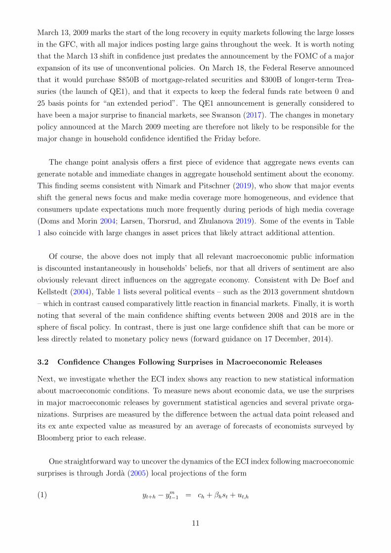
One of the most important economic releases in the U.S is the monthly report on the

Employment Situation by the Bureau of Labor Statistics (BLS). Figure 3 shows the confidence

dynamics associated with the monthly BLS jobs report. Panel 3a shows estimates based on con-

ventional local projections as in (1), whereas Panel 3b shows those obtained from its smoothed

version in (2). Both panels show the ECI index conditional on a one standard deviation nega-

tive surprise in the official unemployment rate (meaning a higher-than-expected unemployment

rate) and in the number of nonfarm payrolls. Panel 3a provides the local projection estimates

together with 68% and 90% confidence bands based on the equal-weighted cosines long-run

variance estimator and optimal bandwidth recommended by Lazarus et al. (2018). For com-

parison, the broken lines in Panel 3a show the smoothed estimates and the associated Lazarus

et al. (2018) 90% bands. The latter are repeated in Panel 3b, which also shows the 68% bands.

Both approaches yield similar findings, and for ease of interpretation we focus on the smoothed

estimates in Panel 3b. Note that the pre-announcement response is mechanically zero for the

smooth projections given the definition of ymt−1.

12Varying the averaging window does not matter much for the qualitative results.

12

(a) Local Projections

-2 0 2 4 6 8 10 12 14 16 18 20

# Days Since Release

-2

-1.5

-1

-0.5

0

0.5

1

1.5

2

Inde

x P

oint

s C

hang

e in

Con

fiden

ce

BLS Unemployment Rate

Day

of R

elea

se

-2 0 2 4 6 8 10 12 14 16 18 20

# Days Since Release

-2

-1.5

-1

-0.5

0

0.5

1

1.5

2

Inde

x P

oint

s C

hang

e in

Con

fiden

ce

BLS Payroll Employment

Day

of R

elea

se

(b) Smooth Projections

-2 0 2 4 6 8 10 12 14 16 18 20

# Days Since Release

-2

-1.5

-1

-0.5

0

0.5

1

1.5

2

Inde

x P

oint

s C

hang

e in

Con

fiden

ce

BLS Unemployment Rate

Day

of R

elea

se

-2 0 2 4 6 8 10 12 14 16 18 20

# Days Since Release

-2

-1.5

-1

-0.5

0

0.5

1

1.5

2

Inde

x P

oint

s C

hang

e in

Con

fiden

ce

BLS Payroll Employment

Day

of R

elea

se

Figure 3: Confidence Dynamics Following One Standard Deviation Surprises in the Jobs Report

Notes: Estimates based on local projections (1) and smooth projections (2) of the daily Gallup ECI index onthe data release minus the consensus forecast. In both panels, shaded areas denote 68% and 90% Lazarus et al.(2018) confidence intervals. For the left panel, dashed lines represent point estimates from smooth projectionsin (2) for comparison, with dot-dash lines corresponding to 90% confidence intervals.

The key result in Figure 3 is that a disappointing jobs report is associated with an immediate

and persistent reduction in household confidence as measured by the daily Gallup ECI. A one

standard deviation miss in the unemployment rate lowers the ECI index by about half a point.

A positive surprise in the payroll number increases confidence by a very similar amount.13 The

confidence changes following surprises in the jobs report are statistically significant at conven-

tional levels for the unemployment rate for nearly two weeks and marginally significant for

payroll employment throughout the month.

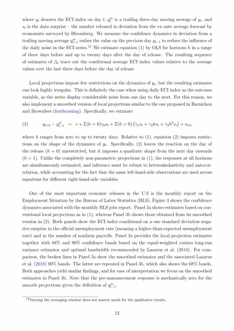
Appendix A.1 presents the results for a number of other major official statistical releases: the

monthly BLS report on CPI inflation, the Bureau of Economic Analysis’ reports on GDP, per-

sonal income, consumption and PCE inflation, Census Bureau releases on retail sales, housing

starts and factory orders, the industrial production numbers released by the Federal Reserve,

and several private releases: the ISM indices, the ADP payroll report, and the Michigan and

13Both the unemployment rate and the payrolls number are part of the same report, and surprises in eachare obviously highly correlated. The confidence effects are therefore not additive.

13

Conference Board consumer confidence indices. A few other macroeconomic releases generate

immediate and persistent confidence changes that are statistically significant. Besides the BLS

jobs report, surprises in the advance GDP report seem to have a meaningful confidence impact,

see the left panel in Figure 4a. A one standard-deviation positive surprise in advance GDP

leads to the largest estimated change in confidence of all releases, persistently raising the ECI

index by between 0.5 and 1 index point. Surprises in the ADP National Employment Report –

a private estimate of national payrolls released a few days ahead of the BLS jobs report– also

appear to have an immediate impact, albeit with effects that are more transitory, see the right

panel in Figure 4a.

A number of releases are followed by gradual changes in confidence that become statistically

significant after a few days or weeks, but without any significant jump in confidence on the

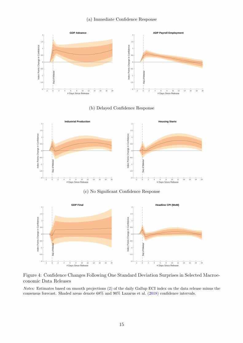
same or subsequent day of the release. Figure 4c provides two examples: industrial production

and housing starts. Positive surprises in these and other releases are of course signals of an

accelerating economy, which also manifests itself as a rise in consumer confidence. The lack

of any instantaneous change in consumer confidence, however, suggest there is no immediate

informational effect on household beliefs at the time of the data surprise. Finally, for many

releases there is no evidence of any systematic change in consumer confidence over the horizons

we consider. Figure 4c provides two examples: the final GDP release and the CPI inflation rate.

While household confidence clearly does not respond to every single new piece of macroe-

conomic information, the evidence above shows that a select few important economic statistics

influence household beliefs about the economy. These are primarily the advance GDP growth

and the jobs numbers, which arguably also receive the broadest and most regular coverage in

the media. The significant high frequency relationship between changes in confidence indicators

and certain data surprises shows the potential for a relatively fast adjustment in beliefs to new

macroeconomic information.

3.3 Information Stickiness in Daily Confidence Data

Another way to assess the responsiveness of household confidence to aggregate news is to see

how closely the daily ECI index tracks information in financial variables and other daily eco-

nomic indicators. To do this, we adapt the methodology of Carroll (2003) and estimate the

degree of ‘stickiness’ in the ECI index relative to other fast-moving high frequency economic

data. The approach is related but distinct from Coibion and Gorodnichenko (2015), who de-

velop measures of informational rigidities based on regression of forecast errors on forecast

revisions. Unfortunately, the Gallup survey data does not have the required information for

such an approach. We therefore do not test departures from full information rational expec-

tations as generally as Coibion and Gorodnichenko (2015). Instead, what we measure is the

stickiness of daily household beliefs relative to information available in daily economic and fi-

nancial indicators, which itself may still be noisy translation of economic fundamentals.

14

(a) Immediate Confidence Response

-2 0 2 4 6 8 10 12 14 16 18 20

# Days Since Release

-2

-1.5

-1

-0.5

0

0.5

1

1.5

2

Inde

x P

oint

s C

hang

e in

Con

fiden

ce

GDP Advance

Day

of R

elea

se

-2 0 2 4 6 8 10 12 14 16 18 20

# Days Since Release

-2

-1.5

-1

-0.5

0

0.5

1

1.5

2

Inde

x P

oint

s C

hang

e in

Con

fiden

ce

ADP Payroll Employment

Day

of R

elea

se

(b) Delayed Confidence Response

-2 0 2 4 6 8 10 12 14 16 18 20

# Days Since Release

-2

-1.5

-1

-0.5

0

0.5

1

1.5

2

Inde

x P

oint

s C

hang

e in

Con

fiden

ce

Industrial Production

Day

of R

elea

se

-2 0 2 4 6 8 10 12 14 16 18 20

# Days Since Release

-2

-1.5

-1

-0.5

0

0.5

1

1.5

2

Inde

x P

oint

s C

hang

e in

Con

fiden

ce

Housing Starts

Day

of R

elea

se

(c) No Significant Confidence Response

-2 0 2 4 6 8 10 12 14 16 18 20

# Days Since Release

-2

-1.5

-1

-0.5

0

0.5

1

1.5

2

Inde

x P

oint

s C

hang

e in

Con

fiden

ce

GDP Final

Day

of R

elea

se

-2 0 2 4 6 8 10 12 14 16 18 20

# Days Since Release

-2

-1.5

-1

-0.5

0

0.5

1

1.5

2

Inde

x P

oint

s C

hang

e in

Con

fiden

ce

Headline CPI (MoM)

Day

of R

elea

se

Figure 4: Confidence Changes Following One Standard Deviation Surprises in Selected Macroe-conomic Data Releases

Notes: Estimates based on smooth projections (2) of the daily Gallup ECI index on the data release minus theconsensus forecast. Shaded areas denote 68% and 90% Lazarus et al. (2018) confidence intervals.

15

To motivate our empirical approach, suppose the vector of relevant economic fundamentals

x∗t evolves according to

x∗t = Ax∗t−1 + ηt , ηt ∼ N(0,Ση).(3)

The true fundamentals x∗t are not (necessarily) directly observed by financial market partici-

pants or any other agent in the economy. Instead, all observable data in period t is measured

by a vector zt

zt = Cx∗t + vt , vt ∼ N(0,Σv),(4)

where vt is a vector of noise. Define the rational (noisy) belief xt = E[x∗t | Zt] where E[·]denotes the mathematical expectation and Zt is the history of observables zt, zt−1, .... This

rational belief xt evolves according to

xt = Axt−1 +Kut,(5)

where K is the Kalman gain and ut is the one step ahead forecast error of zt given history Zt−1:

ut = zt − E [zt | Zt−1] = zt −Bxt−1 , B = CA.(6)

Actual household beliefs about economic fundamentals, denoted by xbt , are not necessarily

rational. Following Mankiw and Reis (2002), suppose only a fraction λ of households update

to the rational belief every period while a fraction 1−λ acquire no new information and simple

project their beliefs forward by Axbt−1. This results in

xbt = λAxbt−1 + (1− λ)xt , 0 ≤ λ ≤ 1.(7)

where xbt are the average household beliefs. Suppose that the confidence index yt depends on

beliefs xbt through

yt = φ′xbt + εt , εt ∼ N(0,Σε),(8)

where εt is an i.i.d. measurement/sampling error. This implies that

yt = λφ′Axbt−1 + (1− λ)yRBt + εt(9)

where yRBt = φ′xt is the confidence index for agents with updated rational economic beliefs.

Neither φ′Axbt−1 nor yRBt is observed directly, so we need additional assumptions to measure

both objects and estimate λ. First, we assume that φ′Axbt−1 ≈ φ′xbt−1 = yt−1 − εt−1. This

assumption means that average confidence in the economy among agents that do not receive

an information update today is very close to average confidence in the economy yesterday.

16

This seems reasonable given the daily frequency of the data. Second, we extract xt from the

observable information zt. Provided that (I − (A −KB)L) is invertible in the past, i.e. that

(I − (A−KB)L)−1 only has positive powers in the lag operator L, the following is true:

xt = (I − (A−KB)L)−1Kzt.(10)

This expression states that all information in xt is spanned by the current and lagged values of

the observables. Our assumptions lead to the following ARMAX(1,1) model for yt:

yt = λyt−1 +M(L)zt + εt − λεt−1 , M(L) = (1− λ)φ′(I − (A−KB)L)−1K(11)

We use the method of Hannan and Rissanen (1982) to estimate λ. The vector of observables

zt includes a large vector of mostly financial market variables (and their lagged variables) as

controls. Specifically, zt contains daily observations on the following: Treasury rates with ma-

turities of 3 months, 1 year, 2 years, and 10 years; futures implied Federal Funds rates at the

next FOMC meeting and in 12 months, the S&P500 index, BAA and AAA-rated corporate

bond yields, the CBOE VIX index, the trade-weighted dollar exchange rate, WTI crude oil

prices, the US Gulf Coast Conventional Gasoline Regular Spot Price, the CRB Spot Commod-

ity Price Index, the Aruoba, Diebold, and Scotti (2009) daily index of economic activity, and

the Baker, Bloom, and Davis (2016) daily economic policy uncertainty index. To determine

the number of lags of zt, we follow the AIC criterion for a daily VAR in zt for all trading days

between January 1, 2008 to December 31, 2017, which results in a lag length of 16 days. We

estimate (11) using all available observations of yt including weekends and holidays. We use

the latest available observations to replace missing observations in zt on weekends and holidays.

Existing estimates of the degree of information stickiness based on lower frequency data

typically typical find that agents update beliefs very infrequently. Based on data from the

Michigan survey, for example, Carroll (2003) estimates that the average duration between up-

dates of household inflation expectations to those of professional forecasters is one year. The

estimates in Coibion and Gorodnichenko (2015) imply an average duration between updates of

inflation expectations by Michigan survey respondents between 5 and 6 months.14

Table 2 presents our estimates of the information stickiness parameter λ based on the higher

frequency different Gallup survey measures. The estimates imply updating rates that are much

higher than in Carroll (2003) or Coibion and Gorodnichenko (2015). Panel (a) in Table 2

shows that the estimate based on the headline ECI index is λ = 0.92. This value implies that

the average time between information updates regarding economic conditions is 1/(1-0.92), or

12.5 days. For the index based on the question about current economic conditions only, this

average duration is 1/(1-0.8), or 5 days. For the index based on question about the direction

14 Coibion and Gorodnichenko (2015) find even slower rates of information updating for professional forecast-ers, and that the updating rates for these forecasters vary importantly across macroeconomic variables.

17

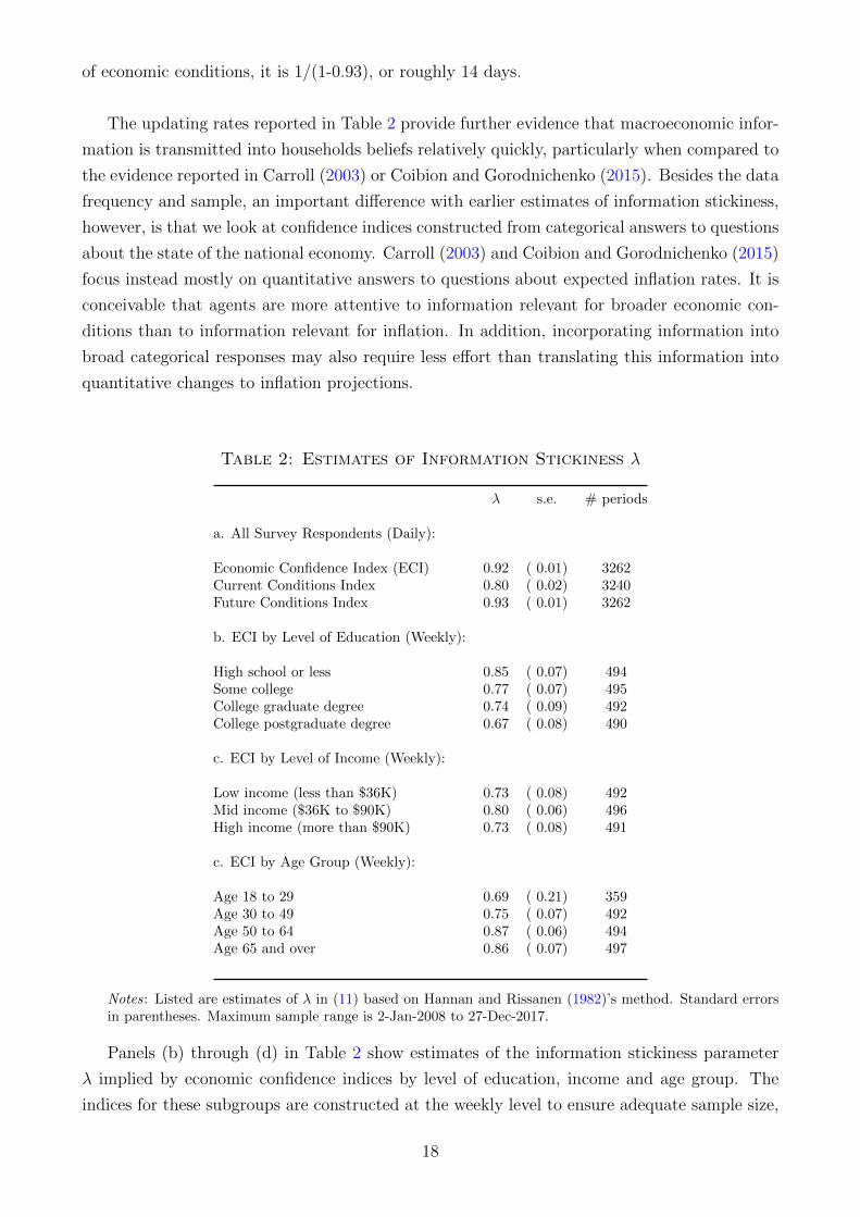
of economic conditions, it is 1/(1-0.93), or roughly 14 days.

The updating rates reported in Table 2 provide further evidence that macroeconomic infor-

mation is transmitted into households beliefs relatively quickly, particularly when compared to

the evidence reported in Carroll (2003) or Coibion and Gorodnichenko (2015). Besides the data

frequency and sample, an important difference with earlier estimates of information stickiness,

however, is that we look at confidence indices constructed from categorical answers to questions

about the state of the national economy. Carroll (2003) and Coibion and Gorodnichenko (2015)

focus instead mostly on quantitative answers to questions about expected inflation rates. It is

conceivable that agents are more attentive to information relevant for broader economic con-

ditions than to information relevant for inflation. In addition, incorporating information into

broad categorical responses may also require less effort than translating this information into

quantitative changes to inflation projections.

Table 2: Estimates of Information Stickiness λ

λ s.e. # periods

a. All Survey Respondents (Daily):

Economic Confidence Index (ECI) 0.92 ( 0.01) 3262Current Conditions Index 0.80 ( 0.02) 3240Future Conditions Index 0.93 ( 0.01) 3262

b. ECI by Level of Education (Weekly):

High school or less 0.85 ( 0.07) 494Some college 0.77 ( 0.07) 495College graduate degree 0.74 ( 0.09) 492College postgraduate degree 0.67 ( 0.08) 490

c. ECI by Level of Income (Weekly):

Low income (less than $36K) 0.73 ( 0.08) 492Mid income ($36K to $90K) 0.80 ( 0.06) 496High income (more than $90K) 0.73 ( 0.08) 491

c. ECI by Age Group (Weekly):

Age 18 to 29 0.69 ( 0.21) 359Age 30 to 49 0.75 ( 0.07) 492Age 50 to 64 0.87 ( 0.06) 494Age 65 and over 0.86 ( 0.07) 497

Notes: Listed are estimates of λ in (11) based on Hannan and Rissanen (1982)’s method. Standard errorsin parentheses. Maximum sample range is 2-Jan-2008 to 27-Dec-2017.

Panels (b) through (d) in Table 2 show estimates of the information stickiness parameter

λ implied by economic confidence indices by level of education, income and age group. The

indices for these subgroups are constructed at the weekly level to ensure adequate sample size,

18

and the estimates are therefore based on weekly rather than daily data. Panel (b) shows that

informational rigidities are decreasing in education level and increasing in age. The point

estimates in Panel (c) suggest that rigidities are greater for mid-income groups than for low-

or high-income groups. While we cannot reject that the estimates are equal across the age

or income groups with much confidence, the estimates by education level are more sharply

different.

4 The Response of Economic Confidence to Monetary Policy News

The evidence in the previous section indicates that public confidence in the state of the aggre-

gate economy can be quite responsive to new macroeconomic information. We now turn to our

main question, does consumer confidence also respond meaningfully to news about monetary

policy? More specifically, our goal is to establish whether monetary policy announcements have

immediate effects on individuals’ assessments of the economic outlook, i.e. upon the arrival of

the news or in the days immediately afterwards. Any instantaneous confidence effects can be,

in our view, only interpreted as a direct reaction to news about monetary policy. The public

may learn this news directly from (media coverage of) central bank communications or from

the reaction in asset markets, even without necessarily fully understanding the origins of this

reaction. However, immediate confidence effects cannot arise from any of subsequent macroe-

conomic effects of the monetary policy announcement itself, for instance through reactions to

unemployment or GDP statistics or changes in individuals’ own labor market status.

To measure monetary policy news, we follow a large empirical literature and assume that

unexpected changes in interest rates shortly after FOMC announcements arise entirely due

to information released by the Federal Reserve.15 While this assumption is relatively uncon-

troversial, the nature of the monetary news being measured using this approach is not fully

clear. On the one hand, news of tighter-than-expected monetary policy can lead agents to

become more pessimistic about economic conditions because of all of the conventional channels

through which a monetary policy shock has contractionary effects. On the other hand, agents

may alternatively view an unexpected tightening by the FOMC as a signal of internal views of

greater-than-expected economic strength, and therefore adjust their beliefs about the economic

conditions upward. Based on the direction of the reactions in financial markets and in surveys

of professional forecasters, there is much evidence that monetary policy news is at least in part

interpreted as internal Fed information about the economy.16 From the short run reaction in

the daily ECI index, we are able to assess in what direction the beliefs of the wider public –

not just of small number of professional forecasters – react to monetary policy news.

Monetary policy news identified using the high frequency approach during the 2008-2017

15See for instance Cook and Hahn (1989), Kuttner (2001), Cochrane and Piazzesi 2002, and Gertler andKaradi (2015)

16See for instance Romer and Romer (2000), Campbell et al. (2012), Nakamura and Steinsson (2018), Miranda-Agrippino and Ricco (2015), Jarociski and Karadi (2018), Lunsford (2018) or Cieslak and Schrimpf (2019).

19

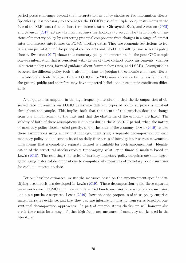
period poses challenges beyond the interpretation as policy shocks or Fed information effects.

Specifically, it is necessary to account for the FOMC’s use of multiple policy instruments in the

face of the ZLB constraint on short term interest rates. Gurkaynak, Sack, and Swanson (2005)

and Swanson (2017) extend the high frequency methodology to account for the multiple dimen-

sions of monetary policy by extracting principal components from changes in a range of interest

rates and interest rate futures on FOMC meeting dates. They use economic restrictions to iso-

late a unique rotation of the principal components and label the resulting time series as policy

shocks. Swanson (2017) shows that monetary policy announcements in the post GFC sample

conveys information that is consistent with the use of three distinct policy instruments: changes

in current policy rates, forward guidance about future policy rates, and LSAPs. Distinguishing

between the different policy tools is also important for judging the economic confidence effects.

The additional tools deployed by the FOMC since 2008 were almost certainly less familiar to

the general public and therefore may have impacted beliefs about economic conditions differ-

ently.

A ubiquitous assumption in the high-frequency literature is that the decomposition of ob-

served rate movements on FOMC dates into different types of policy surprises is constant

throughout the sample. This implies both that the nature of the surprises does not change

from one announcement to the next and that the elasticities of the economy are fixed. The

validity of both of these assumptions is dubious during the 2008-2017 period, when the nature

of monetary policy shocks varied greatly, as did the state of the economy. Lewis (2019) relaxes

these assumptions using a new methodology, identifying a separate decomposition for each

monetary policy announcement based on daily time series of intraday interest rate movements.

This means that a completely separate dataset is available for each announcement. Identifi-

cation of the structural shocks exploits time-varying volatility in financial markets based on

Lewis (2018). The resulting time series of intraday monetary policy surprises are then aggre-

gated using historical decompositions to compute daily measures of monetary policy surprises

for each announcement date.

For our baseline estimates, we use the measures based on the announcement-specific iden-

tifying decompositions developed in Lewis (2019). These decompositions yield three separate

measures for each FOMC announcement date: Fed Funds surprises, forward guidance surprises,

and asset purchase surprises. Lewis (2019) shows that the properties of these policy surprises

match narrative evidence, and that they capture information missing from series based on con-

ventional decomposition approaches. As part of our robustness checks, we will however also

verify the results for a range of other high frequency measures of monetary shocks used in the

literature.

20

4.1 Benchmark Estimates of the Aggregate Confidence Response

To assess the response of consumer sentiment to monetary policy news, we apply the same

local projection methodology that we used in Section 3.2 to estimate the confidence dynamics

around surprises in macroeconomic data releases. Specifically, we estimate

yt+h − ymt−1 = ch + βffh mfft + βfgh m

fgt + βaph m

apt + ut,h(12)

where yt is the ECI index on day t, ymt is a trailing three-day moving average of yt, and mfft , mfg

t

and mapt are the Lewis (2019) monetary policy surprises to the funds rate, forward guidance,

and asset purchases instruments, respectively. The identification based on time-varying volatil-

ity used to derive the policy surprises does not impose that they are orthogonal. We therefore

include all three measures simultaneously in (12) to account for the fact that surprises to the

multiple dimensions of policy routinely occur together.

As before, we also estimate smoothed versions of the local projections:

yt+h − ymt−1 = c+∑

i=ff,fg,ap

[I(h = 0)γi0m

it + I(h > 0)

(γi1 + γi2h+ γi3h

2)mit

]+ ut,h(13)

For both specifications, we compute responses at daily horizons up to four weeks, and we scale

the impulses to correspond to a 25 basis point change in a reference rate, on average, with the

reference rates being the Fed Funds rate for mfft , the 2-year Treasury rate for mfg

t , and the

10-year Treasury rate for mapt .

Figure 5 reports the results. Panel 5a displays local projections, with smooth local pro-

jections and associated 90% Lazarus et al. (2018) confidence intervals for reference; Panel 5b

plots the smooth projections with 68% and 90% confidence intervals. The smooth projections

reinforce patterns already apparent in the non-parametric results.

Our first main finding is a strong and highly significant negative response of economic con-

fidence to a positive surprise in the Fed Funds target, see the left panel in Figure 5. A 25 basis

point surprise hike in the target rate lowers the ECI index by about 1.1 index points on impact,

and by up to 2.6 points after three weeks. These responses, which are on the same scale as the

Michigan Index of Consumer Sentiment, are sizable. The immediate ECI impact, for instance,

corresponds to around 9% of the one day confidence drop following the Lehman bankruptcy,

see Table 1. Another notable feature of the response to a surprise target rate hike is that it

lowers economic confidence. This indicates that, over our sample period, the broader public

interprets positive target surprises as contractionary policy shocks rather than as positive Fed

information about economic conditions. This is consistent with Lewis (2019), who finds based

on the asset price reactions that the policy surprises do not appear to conflate policy news with

Fed information effects.

21

(a) Local Projections

(b) Smooth Projections

Figure 5: Confidence Impact of Monetary Policy Surprises

Notes: Estimates based on local projections (12) and smooth projections (13) of the daily Gallup ECI indexon the monetary policy surprises constructed in Lewis (2019). In both panels, shaded areas denote 68% and90% Lazarus et al. (2018) confidence intervals. For the upper panel, dashed lines represent point estimatesfrom smooth projections in (13) for comparison, with dot-dash lines corresponding to 90% confidence intervals.Responses are scaled to a shock corresponding to a 25 basis-point increase in the respective reference rate: theeffective funds rate in case of a funds rate surprise, the 2 year Treasury rate for forward guidance, and the 10year Treasury rate for the asset purchases.

The other main result is that surprises in the forward guidance or asset purchase instru-

ments do not have similarly clear and pronounced short run confidence effects, see the middle

and right panels in Figure 5. Contractionary forward guidance that results in a 25 basis points

surprise increase in the 2 year Treasury yield lowers confidence by about 5.8 points on impact,

an estimate that is significant at the 90% level. However, in contrast to the target surprise the

confidence effect of forward guidance is almost fully reversed the next day. Economic confi-

dence gradually declines in subsequent days, but remains insignificant for the first three weeks

after the announcement. Recall that the change point analysis in Section 3.1 identified a large

upward jump in confidence on in December 2014 in part on a news headline of a pledged by

22

the Federal Reserve to be patient in raising interest rates. The regression evidence on the con-

fidence impact of forward guidance over the entire sample suggests that such confidence effects

are not clearly systematically a feature of forward guidance announcements.

Interestingly, a surprise asset purchase announcement that raises the 10 year yield by 25

basis point leads to an improvement in economic confidence, see the right panel of Figure 5.

The positive confidence effect of a tightening through asset purchases indicates that Fed infor-

mation effects around LSAP announcements may dominate the policy-inclination effects over

our sample period. However, the response to LSAP surprises is imprecisely estimated and at

best only marginally statistically significant at very short horizons.

In Appendix A.2, we repeat the analysis for the indices based on the separate responses to

the survey questions about the ‘current state’ and ‘direction’ of the national economy, see Sec-

tion 2. There are some indications of a relatively stronger response of the more forward looking

‘directions’ component to forward guidance surprises. In general, however, we find that the re-

sponses to the monetary surprises are very similar across both subcomponents of the ECI index.

We view the results in Figure 5 as evidence that information about monetary policy can

be transmitted to households more directly and quickly than commonly assumed. However,

not all monetary policy news is equal in this regard: only news about the target rate instru-

ment results in clear and unambiguous instantaneous effects in survey measures of household

confidence. Information about the future path of interest rates or asset purchases may not

be transmitted as effectively to the wider public and/or more easily confused with information

about non-monetary fundamentals. That the confidence impact of central bank communication

depends on the monetary policy instrument is perhaps not too surprising. The Federal Funds

target is a long-standing policy tool with which both the media and the wider public is more

likely to be familiar. Additionally, changes in the target rate have been typically communicated

via a single headline leading each FOMC announcement. Communications about forward guid-

ance and asset purchases have arguably been much more challenging, and their effects on the

economy remain relatively poorly understood even among professionals and academics.

Finally, an important implication of our results is that the transmission of target rate

surprises may operate at least in part through a direct and immediate effect on household

confidence, but also that achieving similar effects with other policy instruments may require

further improvements in central bank communication.

4.2 Robustness

In this section, we show that our results on the short run confidence effects of monetary policy

are robust to using an alternative daily indicator of household confidence, and to alternative

high frequency measures of monetary policy news.

23

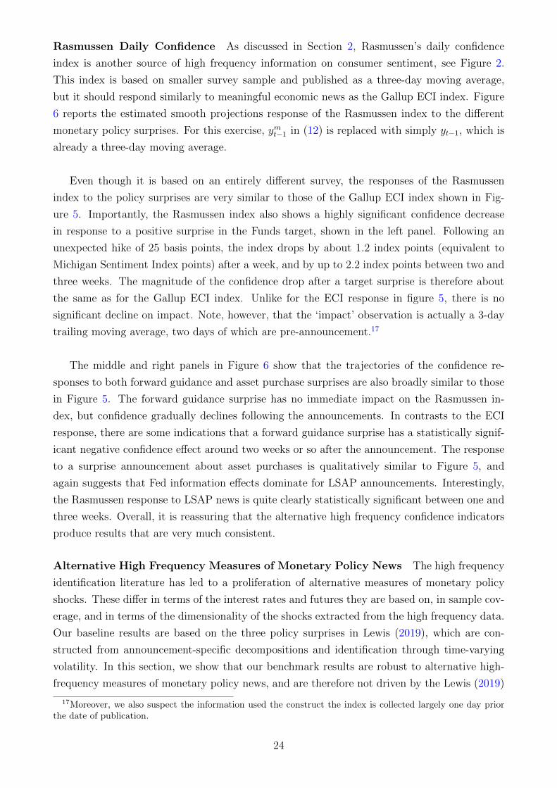
Rasmussen Daily Confidence As discussed in Section 2, Rasmussen’s daily confidence

index is another source of high frequency information on consumer sentiment, see Figure 2.

This index is based on smaller survey sample and published as a three-day moving average,

but it should respond similarly to meaningful economic news as the Gallup ECI index. Figure

6 reports the estimated smooth projections response of the Rasmussen index to the different

monetary policy surprises. For this exercise, ymt−1 in (12) is replaced with simply yt−1, which is

already a three-day moving average.

Even though it is based on an entirely different survey, the responses of the Rasmussen

index to the policy surprises are very similar to those of the Gallup ECI index shown in Fig-

ure 5. Importantly, the Rasmussen index also shows a highly significant confidence decrease

in response to a positive surprise in the Funds target, shown in the left panel. Following an

unexpected hike of 25 basis points, the index drops by about 1.2 index points (equivalent to

Michigan Sentiment Index points) after a week, and by up to 2.2 index points between two and

three weeks. The magnitude of the confidence drop after a target surprise is therefore about

the same as for the Gallup ECI index. Unlike for the ECI response in figure 5, there is no

significant decline on impact. Note, however, that the ‘impact’ observation is actually a 3-day

trailing moving average, two days of which are pre-announcement.17

The middle and right panels in Figure 6 show that the trajectories of the confidence re-

sponses to both forward guidance and asset purchase surprises are also broadly similar to those

in Figure 5. The forward guidance surprise has no immediate impact on the Rasmussen in-

dex, but confidence gradually declines following the announcements. In contrasts to the ECI

response, there are some indications that a forward guidance surprise has a statistically signif-

icant negative confidence effect around two weeks or so after the announcement. The response

to a surprise announcement about asset purchases is qualitatively similar to Figure 5, and

again suggests that Fed information effects dominate for LSAP announcements. Interestingly,

the Rasmussen response to LSAP news is quite clearly statistically significant between one and

three weeks. Overall, it is reassuring that the alternative high frequency confidence indicators

produce results that are very much consistent.

Alternative High Frequency Measures of Monetary Policy News The high frequency

identification literature has led to a proliferation of alternative measures of monetary policy

shocks. These differ in terms of the interest rates and futures they are based on, in sample cov-

erage, and in terms of the dimensionality of the shocks extracted from the high frequency data.

Our baseline results are based on the three policy surprises in Lewis (2019), which are con-

structed from announcement-specific decompositions and identification through time-varying

volatility. In this section, we show that our benchmark results are robust to alternative high-

frequency measures of monetary policy news, and are therefore not driven by the Lewis (2019)

17Moreover, we also suspect the information used the construct the index is collected largely one day priorthe date of publication.

24

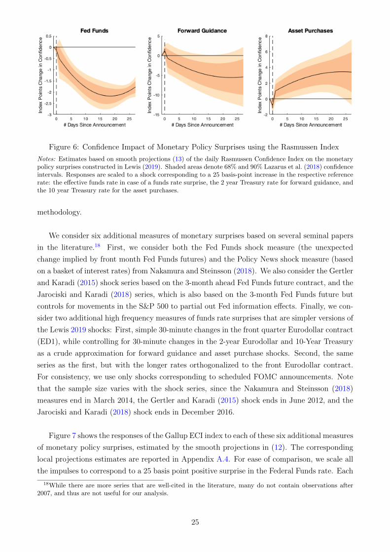
Figure 6: Confidence Impact of Monetary Policy Surprises using the Rasmussen Index

Notes: Estimates based on smooth projections (13) of the daily Rasmussen Confidence Index on the monetarypolicy surprises constructed in Lewis (2019). Shaded areas denote 68% and 90% Lazarus et al. (2018) confidenceintervals. Responses are scaled to a shock corresponding to a 25 basis-point increase in the respective referencerate: the effective funds rate in case of a funds rate surprise, the 2 year Treasury rate for forward guidance, andthe 10 year Treasury rate for the asset purchases.

methodology.

We consider six additional measures of monetary surprises based on several seminal papers

in the literature.18 First, we consider both the Fed Funds shock measure (the unexpected

change implied by front month Fed Funds futures) and the Policy News shock measure (based

on a basket of interest rates) from Nakamura and Steinsson (2018). We also consider the Gertler

and Karadi (2015) shock series based on the 3-month ahead Fed Funds future contract, and the

Jarociski and Karadi (2018) series, which is also based on the 3-month Fed Funds future but

controls for movements in the S&P 500 to partial out Fed information effects. Finally, we con-

sider two additional high frequency measures of funds rate surprises that are simpler versions of

the Lewis 2019 shocks: First, simple 30-minute changes in the front quarter Eurodollar contract

(ED1), while controlling for 30-minute changes in the 2-year Eurodollar and 10-Year Treasury

as a crude approximation for forward guidance and asset purchase shocks. Second, the same

series as the first, but with the longer rates orthogonalized to the front Eurodollar contract.

For consistency, we use only shocks corresponding to scheduled FOMC announcements. Note

that the sample size varies with the shock series, since the Nakamura and Steinsson (2018)

measures end in March 2014, the Gertler and Karadi (2015) shock ends in June 2012, and the

Jarociski and Karadi (2018) shock ends in December 2016.

Figure 7 shows the responses of the Gallup ECI index to each of these six additional measures

of monetary policy surprises, estimated by the smooth projections in (12). The corresponding

local projections estimates are reported in Appendix A.4. For ease of comparison, we scale all

the impulses to correspond to a 25 basis point positive surprise in the Federal Funds rate. Each

18While there are more series that are well-cited in the literature, many do not contain observations after2007, and thus are not useful for our analysis.

25

0 5 10 15 20 25

# Days Since Announcement

-8

-7

-6

-5

-4

-3

-2

-1

0

1

2

Inde

x P

oint

s C

hang

e in

Con

fiden

ce

Nakamura-Steinsson Fed Funds

Day

of F

OM

C

0 5 10 15 20 25

# Days Since Announcement

-5

-4

-3

-2

-1

0

1

Inde

x P

oint

s C

hang

e in

Con

fiden

ce

Nakamura-Steinsson Policy News

Day

of F

OM

C

0 5 10 15 20 25

# Days Since Announcement

-14

-12

-10

-8

-6

-4

-2

0

2

Inde

x P

oint

s C

hang

e in

Con

fiden

ce

Gertler-Karadi

Day

of F

OM

C

0 5 10 15 20 25

# Days Since Announcement

-6

-5

-4

-3

-2

-1

0

1

Inde

x P

oint

s C

hang

e in

Con

fiden

ce

Jarocinski-Karadi

Day

of F

OM

C

0 5 10 15 20 25

# Days Since Announcement

-5

-4

-3

-2

-1

0

1

2

Inde

x P

oint

s C

hang

e in

Con

fiden

ce

30 min. changes in ED1 with long rates

Day

of F

OM

C

0 5 10 15 20 25

# Days Since Announcement

-5

-4

-3

-2

-1

0

1

Inde

x P

oint

s C

hang

e in

Con

fiden

ce

ED1 with orthogonalized long rates

Day

of F

OM

C

Figure 7: Confidence Impact: Alternative Measures of Monetary Policy Shocks

Notes: Estimates based on smooth projections (13) of the daily Gallup ECI index on the monetary policysurprises. Responses are scaled to a shock corresponding to a 25 basis-point increase in the Federal Funds rate.Shaded areas denote 68% and 90% Lazarus et al. (2018) confidence intervals. Dashed lines represent the baselineresponse from the left panel of Figure 5 similarly normalized. Sample periods vary across specification, endingin March 2014 for Nakamura and Steinsson (2018), June 2012 for Gertler and Karadi (2015), and December2016 for Jarociski and Karadi (2018).

panel also shows our baseline estimated ECI response to a funds rate surprise from Figure 5 as

a dashed black line.

The responses in Figure 7 reveal that, independent of the measure used, a positive Federal

Funds surprise always has a negative and statistically significant effect on household confidence.

26

With the exception of the Gertler and Karadi (2015) shocks, the effects are also all of a sim-

ilar magnitude, with a scaled effect peaking at 2-3 index points around 2-3 weeks after the

announcement. For all series, the decrease is significant at least during the first week following

an FOMC announcement. The only notably different results occur for the Gertler and Karadi

(2015) shocks, which exhibit much larger effects reaching 8 to 10 Michigan-Sentiment-equivalent

index points. The much larger responses are likely due to the fact that these shocks only run

until June 2012.19 The overall conclusion is nevertheless that our finding that Federal Funds

target surprises have immediate and significant effects on household confidence is robust to the

use of alternative shock measures.

4.3 The Equity Market Channel

It is unlikely that the confidence responses to surprises in jobs numbers or FOMC interest rate

decisions arise because of widespread public attention to press releases by the Federal Reserve

or the statistical agencies. More plausible is that the public responds to media reporting of

these releases and/or to the reactions in financial markets. Several studies document evidence

for a role of both the volume and tone of media reporting in shaping household expectations.20

However, it is inevitably very difficult to distinguish sharply between media and financial mar-

kets as sources of public information, as events that cause larger financial market reactions are

almost automatically also more newsworthy. While making such a sharp distinction is beyond

the scope of this paper, in this section we explore the role of the stock market response to

macroeconomic news in determining the impact on households confidence. Reactions in the

stock market are arguably one of the most important determinants of media coverage and pub-

lic attention to economic news.

To assess the potential role of an ‘equity market channel’, we modify the local projections

in (1) and smooth projections in (2) to include interactions with equity price changes. In

particular, we estimate local projections of the form

yt+h − ymt−1 = ch + βhst + αhrt + κhstrt + ut,h(14)

as well as its smooth version:

(15)

yt+h − ymt−1 = c+ I(h = 0) (γ0st + φ0rt + ψ0strt)

+ I(h > 0)

((γ1st + γ2hst + γ3h

2st)

+(ψ1strt + ψ2hstrt + ψ3h

2strt))

+ ut,h,

where st is the macroeconomic surprise and rt is an equity price change. We use the daily

log return for the S&P 500 as our measure of equity price change rt. The regression in (15)

19After estimating and rescaling responses for the 2008-2012 sample, we also find larger response to ourbaseline shocks.

20See for instance Carroll (2003), Doms and Morin (2004), Ehrmann, Pfajfar, and Santoro (2017), and Larsen,Thorsrud, and Zhulanova (2019)

27

effectively extends our earlier specification by controlling for the equity price response.

If the daily stock market change rt and the surprise st are uncorrelated, then the responses

estimated by (15) and evaluated at rt = 0 should be approximately be same as those estimated

without controlling for rt. This would indicate that the households response is to information

that is orthogonal to equity price changes. If the responses are changed, but still significant, it

means that there is at least some component of the confidence response that is independent of

the stock market response. Finally, if there is no significant confidence response after control-

ling for stock price changes, this does not necessarily mean that households are only reacting

indirectly to the equity response, but simply that they respond in a similar fashion as the stock

markets.

We estimate the smooth projections augmented with stock price changes in (15) for the

macroeconomic data surprises analyzed in Section 3.2. The full results for all statistical re-

leases are reported in Appendix A.4. The main finding is that for almost all of the twenty

releases we consider, the confidence response after controlling for equity price movements are

virtually unchanged. The job market and advance GDP releases that had significant responses

in the baseline specification also remain significant. On this basis, we can reject the hypothesis

that consumers are solely responding to the equity price movements following macroeconomic

data surprises.

Figure 8 presents the corresponding results for the three monetary policy surprises con-

structed by Lewis (2019). For comparison, the dashed lines represent the baseline responses

reported earlier in section 4.1. For forward guidance and asset purchase surprises, we obtain

very similar results as for the macro data surprises: the point estimates barely change after

controlling for the equity response. However, the left panel shows that the drop in consumer

sentiment following a positive funds rate surprise disappear entirely after controlling for equity

prices. Household confidence and equity markets, therefore respond very similarly to funds

rate surprises. This is consistent with households responding primarily to the stock market

reaction to funds rate surprises, but we cannot rule out that these responses are to equivalent

information obtained elsewhere.

4.4 Heterogeneity in the Confidence Effects of Monetary Policy

The Gallup data allows us to explore possible heterogeneity in the confidence response to mon-

etary surprises. In Section 3.3, we showed that estimates of the degree of information stickiness

decrease with the level of education. It is therefore conceivable that the transmission of infor-

mation about monetary policy decisions varies with the level of education or other demographic

characteristics.

To assess the role of education, we construct separate daily indices for respondents with at

28

Figure 8: Confidence Impact of Monetary Policy Surprises, Controlling for Equity Prices

Notes: Responses are scaled to a shock corresponding to a 25 basis-point increase in the respective referencerate: the effective funds rate in case of a funds rate surprise, the 2 year Treasury rate for forward guidance,and the 10 year Treasury rate for the asset purchases. Shaded areas denote 68% and 90% Lazarus et al. (2018)confidence intervals.

least some college and for those with a high school degree or less. We also construct separate

indices for low and high income individuals, depending on whether household income falls below

or above $60K, and for younger and older survey respondents, by grouping those aged 18-45

and those aged 46 and over. For each of these subindices, we re-estimate the projections in

(12) and (13).

Figure 9 plots the smooth projection results by education level.21 The impulse with orange

confidence intervals is for survey respondents with at least some college education, whereas the

one with green intervals is for the non-college educated. The responses indicate that more highly

educated survey respondents react more strongly to a Fed Funds surprise, with a maximum

decline in confidence of around 3.3 points, about twice as much as the decline in confidence

among the less educated (1.6 points). In Appendix A.6, we show that the difference between the

confidence responses becomes formally statistically significant in the third week following the

funds rate surprise. The responses to forward guidance and asset purchase surprises are broadly

similar among education groups. As in the aggregate results in Figure 5, the pronounced and

strongly significant short run confidence effects associated with funds rate surprises are gener-

ally absent for the other policy instruments. However, more educated individuals do exhibit a

significant decline in confidence following forward guidance on impact and also after 3 weeks

or so. The confidence impact of forward guidance for the less educated, in contrast, is never

statistically significant. The responses to news about asset purchases are not significant for ei-

ther education group. The impact response to asset purchase surprises, however, is significantly

lower among the more highly educated, see Appendix A.6. While the estimates are inevitably

somewhat imprecise, our overall conclusion is that are indications of larger confidence reactions

to monetary policy news among the more highly educated. This is consistent with greater levels

of attention to monetary policy news, and is consistent with the results of Section 3.3.

21The local projections results for every education, income and age group are provided in Appendix A.5.

29

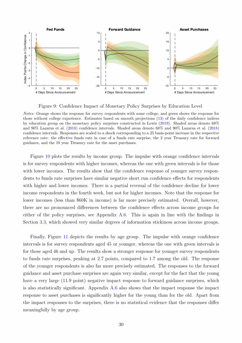
Figure 9: Confidence Impact of Monetary Policy Surprises by Education Level

Notes: Orange shows the response for survey respondents with some college, and green shows the response forthose without college experience. Estimates based on smooth projections (13) of the daily confidence indicesby education group on the monetary policy surprises constructed in Lewis (2019). Shaded areas denote 68%and 90% Lazarus et al. (2018) confidence intervals. Shaded areas denote 68% and 90% Lazarus et al. (2018)confidence intervals. Responses are scaled to a shock corresponding to a 25 basis-point increase in the respectivereference rate: the effective funds rate in case of a funds rate surprise, the 2 year Treasury rate for forwardguidance, and the 10 year Treasury rate for the asset purchases.

Figure 10 plots the results by income group. The impulse with orange confidence intervals

is for survey respondents with higher incomes, whereas the one with green intervals is for those

with lower incomes. The results show that the confidence response of younger survey respon-

dents to funds rate surprises have similar negative short run confidence effects for respondents

with higher and lower incomes. There is a partial reversal of the confidence decline for lower

income respondents in the fourth week, but not for higher incomes. Note that the response for

lower incomes (less than $60K in income) is far more precisely estimated. Overall, however,

there are no pronounced differences between the confidence effects across income groups for

either of the policy surprises, see Appendix A.6. This is again in line with the findings in

Section 3.3, which showed very similar degrees of information stickiness across income groups.

Finally, Figure 11 depicts the results by age group. The impulse with orange confidence

intervals is for survey respondents aged 45 or younger, whereas the one with green intervals is

for those aged 46 and up. The results show a stronger response for younger survey respondents

to funds rate surprises, peaking at 2.7 points, compared to 1.7 among the old. The response

of the younger respondents is also far more precisely estimated. The responses to the forward

guidance and asset purchase surprises are again very similar, except for the fact that the young

have a very large (11.9 point) negative impact response to forward guidance surprises, which

is also statistically significant. Appendix A.6 also shows that the impact response the impact

response to asset purchases is significantly higher for the young than for the old. Apart from

the impact responses to the surprises, there is no statistical evidence that the responses differ

meaningfully by age group.

30

Figure 10: Confidence Impact of Monetary Policy Surprises by Income Level

Notes: Orange shows the response of respondents with household incomes exceeding $60K, and green showsthe response for lower incomes. Estimates based on smooth projections (13) of the daily confidence indices byincome group on the monetary policy surprises constructed in Lewis (2019). Shaded areas denote 68% and 90%Lazarus et al. (2018) confidence intervals. Shaded areas denote 68% and 90% Lazarus et al. (2018) confidenceintervals. Responses are scaled to a shock corresponding to a 25 basis-point increase in the respective referencerate: the effective funds rate in case of a funds rate surprise, the 2 year Treasury rate for forward guidance, andthe 10 year Treasury rate for the asset purchases.

In conclusion, there is definitely some evidence of heterogeneity in the confidence response

to monetary surprises. Specifically, better educated and also younger individuals appear to

show a larger decline in confidence following a upward surprise in the funds rate target. The

fact that the results conditional on monetary policy news are broadly in line with the evidence

of heterogeneity in information stickiness reported in Section 3.3 suggest that the heterogeneity

in the confidence responses is linked to heterogeneity in attentiveness to information about

monetary policy decisions.

31

Figure 11: Confidence Impact of Monetary Policy Surprises by Age Group

Notes: Orange shows the response for survey respondents aged 45 or younger, and green shows the responsefor those aged 45 and up. Estimates based on smooth projections (13) of the daily confidence indices by agegroup on the monetary policy surprises constructed in Lewis (2019). Shaded areas denote 68% and 90% Lazaruset al. (2018) confidence intervals. Shaded areas denote 68% and 90% Lazarus et al. (2018) confidence intervals.Responses are scaled to a shock corresponding to a 25 basis-point increase in the respective reference rate: theeffective funds rate in case of a funds rate surprise, the 2 year Treasury rate for forward guidance, and the 10year Treasury rate for the asset purchases.

32

5 Conclusion

In this paper, we provide evidence that surprises in Federal Funds rate decisions generate im-

mediate effects on public confidence in economic conditions. Two key features of our analysis

distinguish it from existing work on the impact of monetary policy on expectations. The first

is that we focus on the impact on the beliefs of the general public rather than of professional

forecasters or financial market participants. The second is that we evaluate confidence reac-

tions at the daily frequency. This means we can more confidently rule out other confounding

factors and satisfy the exclusion restriction implicit in the event study approach. Moreover,

the significant instantaneous confidence response at the daily level establishes that households

change their economic outlook in response to announcements about monetary policy, and not

just after experiencing its later economic impact.

Whereas we find that surprises in the funds rate impact public confidence instantaneously,

we find little evidence for similar effects in response to monetary policy news related to forward

guidance or asset purchases. This finding suggest that there remain significant communication

challenges surrounding the use of these alternative policy instruments, and is consistent with

a broader recognition that there is still ample scope to improve the communication of Federal

Reserve policies, see Orphanides (2019).

Our results imply that information about monetary policy decisions is therefore transmitted

more effectively, through media coverage and/or observation of the asset market reaction, to

the general public than suggested by existing evidence on informational rigidities. Moreover, we

also provide more general evidence that measures of public confidence in the economy respond to

certain types of macroeconomic news relatively quickly. A likely important difference between

our analysis and the existing literature on informational rigidities is that we focus on categorical

survey answers about economic conditions rather than on quantitative inflation expectations.

We conjecture that time aggregation may be an additional reason that the higher frequency

survey data points to more flexible adjustments in beliefs in response to new information. We

plan to pursue this conjecture in future research.

33

References

Aghion, Philippe et al. (2016). “Creative Destruction and Subjective Well-Being”. In: American

Economic Review 106.12, pp. 3869–97. doi: 10.1257/aer.20150338.

Altavilla, Carlo and Domenico Giannone (2017). “The Effectiveness of Non-Standard Monetary

Policy Measures: Evidence from Survey Data”. In: Journal of Applied Econometrics 32.5,

pp. 952–964. doi: 10.1002/jae.2559.

Aruoba, S. Boragan, Francis X. Diebold, and Chiara Scotti (2009). “Real-Time Measurement

of Business Conditions”. In: Journal of Business & Economic Statistics 27.4, pp. 417–427.

doi: 10.1198/jbes.2009.07205.

Baker, Scott R., Nicholas Bloom, and Steven J. Davis (2016). “Measuring Economic Policy

Uncertainty”. In: The Quarterly Journal of Economics 131.4, pp. 1593–1636. doi: 10 .

1093/qje/qjw024.

Barnichon, Regis and Christian Brownlees (forthcoming). “Impulse Response Estimation By

Smooth Local Projections”. In: The Review of Economics and Statistics 0.0, pp. 1–9. doi:

10.1162/rest\_a\_00778.

Binder, Carola (2017). “Federal Reserve Communication and the Media”. In: Journal of Media

Economics 30.4, pp. 191–214. doi: 10.1080/08997764.2018.1515767.

Blinder, Alan S. (2008). Talking about Monetary Policy: The Virtues (and Vices?) of Central

Bank Communication. Working Papers 1048. Princeton University, Department of Eco-

nomics, Center for Economic Policy Studies.

— (2018). “Through a Crystal Ball Darkly: The Future of Monetary Policy Communication”.

In: AEA Papers and Proceedings 108, pp. 567–71. doi: 10.1257/pandp.20181080.

Campbell, Jeffrey R. et al. (2012). “Macroeconomic Effects of Federal Reserve Forward Guid-

ance”. In: Brookings Papers on Economic Activity 43.1 (Spring, pp. 1–80.

Carroll, Christopher D. (2003). “Macroeconomic Expectations of Households and Professional

Forecasters”. In: The Quarterly Journal of Economics 118.1, pp. 269–298. doi: 10.1162/

00335530360535207.

Cieslak, Anna and Andreas Schrimpf (2019). “Non-monetary news in central bank communica-

tion”. In: Journal of International Economics 118, pp. 293 –315. doi: https://doi.org/

10.1016/j.jinteco.2019.01.012.

Cochrane, John H. and Monika Piazzesi (2002). “The Fed and Interest Rates - A High-

Frequency Identification”. In: American Economic Review 92.2, pp. 90–95. doi: 10.1257/

000282802320189069.

Coibion, Olivier and Yuriy Gorodnichenko (2015). “Information Rigidity and the Expectations

Formation Process: A Simple Framework and New Facts”. In: American Economic Review

105.8, pp. 2644–78. doi: 10.1257/aer.20110306.

Coibion, Olivier et al. (2018). Inflation Expectations as a Policy Tool? Working Paper 24788.

National Bureau of Economic Research. doi: 10.3386/w24788.

34

Cook, Timothy and Thomas Hahn (1989). “The effect of changes in the federal funds rate target

on market interest rates in the 1970s”. In: Journal of Monetary Economics 24.3, pp. 331

–351. doi: https://doi.org/10.1016/0304-3932(89)90025-1.

De Boef, Suzanna and Paul M. Kellstedt (2004). “The Political (and Economic) Origins of

Consumer Confidence”. In: American Journal of Political Science 48.4, pp. 633–649. doi:

10.1111/j.0092-5853.2004.00092.x.

Del Negro, Marco, Marc Giannoni, and Christina Patterson (2015). The forward guidance puz-

zle. Tech. rep.

Doms, Mark and Norman J. Morin (2004). Consumer sentiment, the economy, and the news

media. Finance and Economics Discussion Series 2004-51. Board of Governors of the Federal

Reserve System.

Eberly, Janice C, James H Stock, and Jonathan H Wright (2019). The Federal Reserves Current

Framework for Monetary Policy: A Review and Assessment. Working Paper 26002. National

Bureau of Economic Research. doi: 10.3386/w26002.

Ehrmann, Michael, Damjan Pfajfar, and Emiliano Santoro (2017). “Consumers’ Attitudes and

Their Inflation Expectations”. In: International Journal of Central Banking 13.1, pp. 225–

259.

Gertler, Mark and Peter Karadi (2015). “Monetary Policy Surprises, Credit Costs, and Eco-

nomic Activity”. In: American Economic Journal: Macroeconomics 7.1, pp. 44–76. doi:

10.1257/mac.20130329.

Gurkaynak, Refet S, Brian Sack, and Eric Swanson (2005). “Do Actions Speak Louder Than

Words? The Response of Asset Prices to Monetary Policy Actions and Statements”. In:

International Journal of Central Banking 1.1. url: https://ideas.repec.org/a/ijc/

ijcjou/y2005q2a2.html.

Hannan, Edward J. and Jorma Rissanen (1982). “Recursive Estimation of Mixed Autoregressive-

Moving Average Order”. In: Biometrika 69.1, pp. 81–94. doi: 10.2307/2335856.

Jarociski, Marek and Peter Karadi (2018). Deconstructing monetary policy surprises: the role

of information shocks. Working Paper Series 2133. European Central Bank.

Jorda, Oscar (2005). “Estimation and Inference of Impulse Responses by Local Projections”.

In: American Economic Review 95.1, pp. 161–182. doi: 10.1257/0002828053828518.

Kahneman, Daniel and Angus Deaton (2010). “High income improves evaluation of life but

not emotional well-being”. In: Proceedings of the National Academy of Sciences 107.38,

pp. 16489–16493.

Killick, Rebecca, Paul Fearnhead, and Idris A. Eckley (2012). “Optimal Detection of Change-

points With a Linear Computational Cost”. In: Journal of the American Statistical Associ-

ation 107.500, pp. 1590–1598. doi: 10.1080/01621459.2012.737745.

Kuttner, Kenneth N. (2001). “Monetary policy surprises and interest rates: Evidence from the

Fed funds futures market”. In: Journal of Monetary Economics 47.3, pp. 523–544. doi:

10.1016/S0304-3932(01)00055-1.

35

Larsen, Vegard H., Leif Anders Thorsrud, and Julia Zhulanova (2019). News-driven inflation

expectations and information rigidities. Working Paper 5/2019. Norges Bank.

Lazarus, Eben et al. (2018). “HAR Inference: Recommendations for Practice”. In: Journal of

Business & Economic Statistics 36.4, pp. 541–559. doi: 10.1080/07350015.2018.1506926.

Lewis, Daniel J. (2018). Identifying shocks via time-varying volatility. Staff Reports 871. Federal

Reserve Bank of New York.

— (2019). Announcement-Specific Decompositions of Unconventional Monetary Policy Shocks

and Their Macroeconomic Effects. Staff Reports 891. Federal Reserve Bank of New York.

Lucca, David O and Francesco Trebbi (2009). Measuring Central Bank Communication: An

Automated Approach with Application to FOMC Statements. Working Paper 15367. National

Bureau of Economic Research. doi: 10.3386/w15367.

Ludvigson, Sydney C. (2004). “Consumer Confidence and Consumer Spending”. In: Journal of

Economic Perspectives 18.2, pp. 29–50. doi: 10.1257/0895330041371222.

Lunsford, Kurt G. (2018). Tech. rep.

Makridis, Christos (2019). Sentimental Business Cycles and the Protracted Great Recession.

Working paper. MIT Sloan.

Mankiw, N. Gregory and Ricardo Reis (2002). “Sticky Information versus Sticky Prices: A

Proposal to Replace the New Keynesian Phillips Curve*”. In: The Quarterly Journal of

Economics 117.4, pp. 1295–1328. doi: 10.1162/003355302320935034.

Miranda-Agrippino, Silvia and Giovanni Ricco (2015). The Transmission of Monetary Policy

Shocks. Tech. rep. Centre for Macroeconomics (CFM).

Nakamura, Emi and Jon Steinsson (2018). “High-Frequency Identification of Monetary Non-

Neutrality: The Information Effect”. In: The Quarterly Journal of Economics 133.3, pp. 1283–

1330. doi: 10.1093/qje/qjy004.

Nimark, Kristoffer P. and Stefan Pitschner (2019). “News media and delegated information

choice”. In: Journal of Economic Theory 181, pp. 160 –196. doi: https://doi.org/10.

1016/j.jet.2019.02.001.

Orphanides, Athanasios (2019). Monetary Policy Strategy and its Communication. Discussion

Paper. Jackson Hole Economic Policy Symposium.

Romer, Christina D. and David H. Romer (2000). “Federal Reserve Information and the Be-

havior of Interest Rates”. In: American Economic Review 90.3, pp. 429–457. doi: 10.1257/

aer.90.3.429.

Swanson, Eric T. (2017). Measuring the Effects of Federal Reserve Forward Guidance and As-

set Purchases on Financial Markets. NBER Working Papers 23311. National Bureau of

Economic Research. doi: 10.3386/w23311.

36

A Appendix

A.1 Confidence Dynamics Around Macroeconomic Data Surprises

This section provides the full set of estimates of the confidence dynamics surrounding surprises

in macroeconomic data releases, discussed in Section 3.2. Figure 12 depicts the estimates based

on local projections obtained from (1), whereas dashed lines shows the estimates based the

smooth local projections (2).

Table 3 lists the estimated change in confidence relative on (1) the day of the release, (2)

the next day and (3) one week after the release. The releases are in descending order based

on the estimated ECI change on the next day. Standard errors are in parentheses. The point

estimates are based on the smooth projections in (2) and represent the confidence change in

index points associated with a one standard deviation positive surprise. Most of the releases

are monthly with roughly 120 releases over the 10-year sample. The number of observations

roughly equals the number of releases over the sample period times the estimation horizon of

28 days. The sample sizes vary slightly across the releases because of missing observations in

the ECI series (holidays etc.) The weekly initial claims and the GDP reports are at a weekly

and quarterly frequency, and the sample sizes change accordingly. We use a horizon up to 7

days for the weekly claims, and maintain the 21 day window for the GDP reports.

37

Table 3: Confidence Changes Following Surprises in Macro Releases

# releases # obs. Day of Release Next Day Next Week

GDP Advance 40 799 0.85 0.90∗∗∗ 0.59(0.53) (0.25) (0.47)

BLS Unemployment Rate 120 2389 −0.51∗∗ −0.68∗∗∗ −0.52∗

(0.23) (0.22) (0.27)

ADP Payroll Employment 120 2384 0.45∗∗∗ 0.62∗∗∗ 0.39∗∗∗

(0.17) (0.18) (0.11)

BLS Payroll Employment 120 2389 0.24 0.59∗ 0.46∗

(0.34) (0.34) (0.26)

GDP Second 40 784 0.40 0.52 0.75∗∗∗

(0.42) (0.47) (0.29)

ISM Manufacturing 120 2359 0.16 0.47 0.53∗

(0.37) (0.37) (0.30)

Advance Retail Sales 120 2358 0.12 0.39∗ 0.53∗∗∗

(0.29) (0.23) (0.18)

GDP Final 32 584 −0.12 0.33 0.34(0.46) (0.65) (0.53)

Factory Orders 119 2371 0.05 0.33 0.31(0.40) (0.22) (0.40)

Conf Board Confidence 120 2360 0.07 0.29 0.33(0.25) (0.31) (0.30)

Headline CPI (MoM) 120 2337 0.34 −0.19 0.12(0.24) (0.20) (0.17)

Personal Income 120 2325 0.23 0.12 −0.39∗∗∗

(0.23) (0.32) (0.12)

U of.M Sentiment (Final) 120 2325 −0.62∗∗∗ −0.08 −0.21(0.21) (0.25) (0.25)

U of M Confidence (Prelim) 120 2364 0.15 0.08 0.02(0.38) (0.31) (0.27)

Industrial Production 120 2347 0.39 −0.07 0.43(0.31) (0.34) (0.34)

PCE Deflator YoY 120 2325 0.59∗∗ 0.04 0.09(0.30) (0.23) (0.26)

Initial Jobless Claims 522 3416 −0.07 0.03 0.09(0.16) (0.14) (0.21)

Personal Consumption 120 2325 −0.06 0.03 −0.06(0.30) (0.26) (0.23)

Housing Starts 118 2300 0.07 −0.03 0.58∗∗

(0.39) (0.16) (0.28)

ISM Non-Manufacturing 120 2403 0.12 0.01 −0.00(0.31) (0.24) (0.34)

Notes: Estimates based on smooth projections as in (2) of the Gallup ECI on surprises in macroeconomicdata releases. In descending order based on the estimated change on the next day of the release. Standarderrors based on Lazarus et al. (2018) in parenthesis. Asterisks denote 10%, 5% or 1% significance. Samplerange is 2-Jan-2008 to 27-Dec-2017.

38

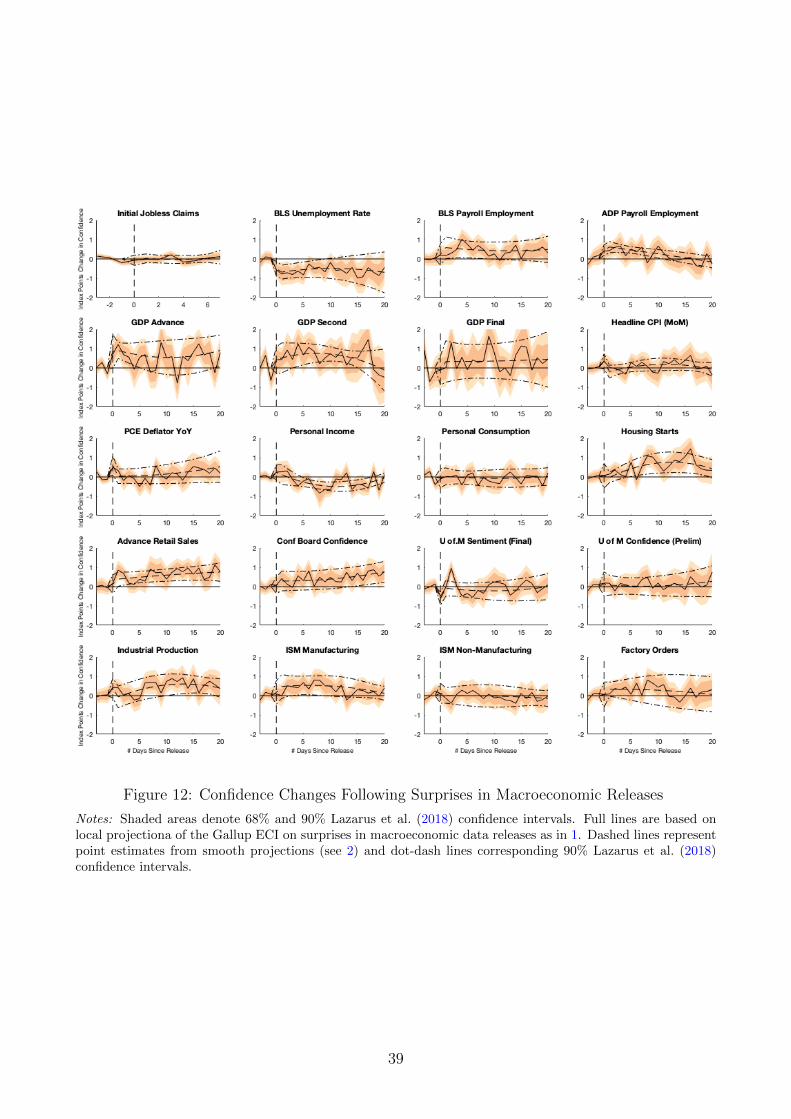
Figure 12: Confidence Changes Following Surprises in Macroeconomic Releases

Notes: Shaded areas denote 68% and 90% Lazarus et al. (2018) confidence intervals. Full lines are based onlocal projectiona of the Gallup ECI on surprises in macroeconomic data releases as in 1. Dashed lines representpoint estimates from smooth projections (see 2) and dot-dash lines corresponding 90% Lazarus et al. (2018)confidence intervals.

39

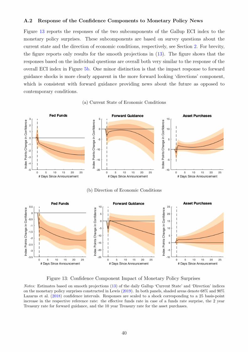
A.2 Response of the Confidence Components to Monetary Policy News

Figure 13 reports the responses of the two subcomponents of the Gallup ECI index to the

monetary policy surprises. These subcomponents are based on survey questions about the

current state and the direction of economic conditions, respectively, see Section 2. For brevity,

the figure reports only results for the smooth projections in (13). The figure shows that the

responses based on the individual questions are overall both very similar to the response of the

overall ECI index in Figure 5b. One minor distinction is that the impact response to forward

guidance shocks is more clearly apparent in the more forward looking ‘directions’ component,

which is consistent with forward guidance providing news about the future as opposed to

contemporary conditions.

(a) Current State of Economic Conditions

(b) Direction of Economic Conditions

Figure 13: Confidence Component Impact of Monetary Policy Surprises

Notes: Estimates based on smooth projections (13) of the daily Gallup ‘Current State’ and ‘Direction’ indiceson the monetary policy surprises constructed in Lewis (2019). In both panels, shaded areas denote 68% and 90%Lazarus et al. (2018) confidence intervals. Responses are scaled to a shock corresponding to a 25 basis-pointincrease in the respective reference rate: the effective funds rate in case of a funds rate surprise, the 2 yearTreasury rate for forward guidance, and the 10 year Treasury rate for the asset purchases.

40

A.3 Local Projection Estimates Using Alternative Monetary Policy Shocks

Figure 14 shows the responses of the ECI index to various measures of monetary policy shocks,

estimated using local projections as in (12).

0 5 10 15 20 25

# Days Since Announcement

-10

-8

-6

-4

-2

0

2

4

Inde

x P

oint

s C

hang

e in

Con

fiden

ce

Nakamura-Steinsson Fed FundsD

ay o

f FO

MC

0 5 10 15 20 25

# Days Since Announcement

-10

-5

0

5

Inde

x P

oint

s C

hang

e in

Con

fiden

ce

Nakamura-Steinsson Policy News

Day

of F

OM

C

0 5 10 15 20 25

# Days Since Announcement

-35

-30

-25

-20

-15

-10

-5

0

5

10

15

Inde

x P

oint

s C

hang

e in

Con

fiden

ce

Gertler-Karadi

Day

of F

OM

C

0 5 10 15 20 25

# Days Since Announcement

-10

-5

0

5

Inde

x P

oint

s C

hang

e in

Con

fiden

ce

Jarocinski-Karadi

Day

of F

OM

C

0 5 10 15 20 25

# Days Since Announcement

-8

-6

-4

-2

0

2

4

6

Inde

x P

oint

s C

hang

e in

Con

fiden

ce

30 min. changes in ED1 with long rates

Day

of F

OM

C

0 5 10 15 20 25

# Days Since Announcement

-10

-5

0

5

Inde

x P

oint

s C

hang

e in

Con

fiden

ce

ED1 with orthogonalized long rates

Day

of F

OM

C

Figure 14: Confidence Impact: Alternative Monetary Policy Shocks

Notes: Estimates based on local projections (12) of the daily Gallup ECI index on the monetary policy surprises.Responses are scaled to a shock corresponding to a 25 basis-point increase in the Fed Funds rate. Shaded areasdenote 68% and 90% Lazarus et al. (2018) confidence intervals. Dashed lines represent point estimates fromsmooth projections and dot-dash lines corresponding 90% confidence intervals. Sample periods vary acrossspecification, ending in March 2014 for Nakamura and Steinsson (2018), June 2012 for Gertler and Karadi(2015), and December 2016 for Jarociski and Karadi (2018).

41

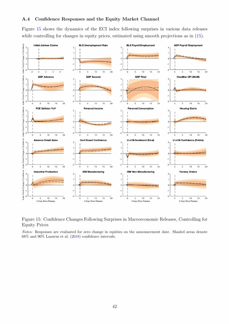
A.4 Confidence Responses and the Equity Market Channel

Figure 15 shows the dynamics of the ECI index following surprises in various data releases

while controlling for changes in equity prices, estimated using smooth projections as in (15).

Figure 15: Confidence Changes Following Surprises in Macroeconomic Releases, Controlling forEquity Prices

Notes: Responses are evaluated for zero change in equities on the announcement date. Shaded areas denote68% and 90% Lazarus et al. (2018) confidence intervals.

42

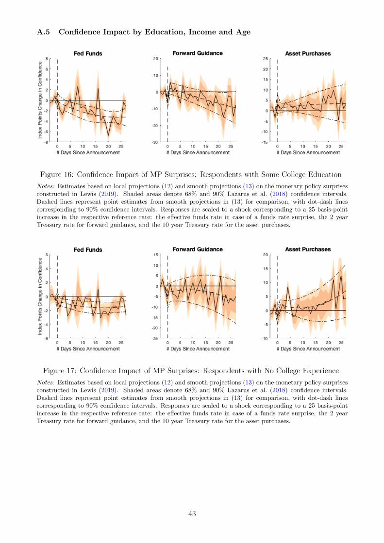
A.5 Confidence Impact by Education, Income and Age

Figure 16: Confidence Impact of MP Surprises: Respondents with Some College Education

Notes: Estimates based on local projections (12) and smooth projections (13) on the monetary policy surprisesconstructed in Lewis (2019). Shaded areas denote 68% and 90% Lazarus et al. (2018) confidence intervals.Dashed lines represent point estimates from smooth projections in (13) for comparison, with dot-dash linescorresponding to 90% confidence intervals. Responses are scaled to a shock corresponding to a 25 basis-pointincrease in the respective reference rate: the effective funds rate in case of a funds rate surprise, the 2 yearTreasury rate for forward guidance, and the 10 year Treasury rate for the asset purchases.

Figure 17: Confidence Impact of MP Surprises: Respondents with No College Experience

Notes: Estimates based on local projections (12) and smooth projections (13) on the monetary policy surprisesconstructed in Lewis (2019). Shaded areas denote 68% and 90% Lazarus et al. (2018) confidence intervals.Dashed lines represent point estimates from smooth projections in (13) for comparison, with dot-dash linescorresponding to 90% confidence intervals. Responses are scaled to a shock corresponding to a 25 basis-pointincrease in the respective reference rate: the effective funds rate in case of a funds rate surprise, the 2 yearTreasury rate for forward guidance, and the 10 year Treasury rate for the asset purchases.

43

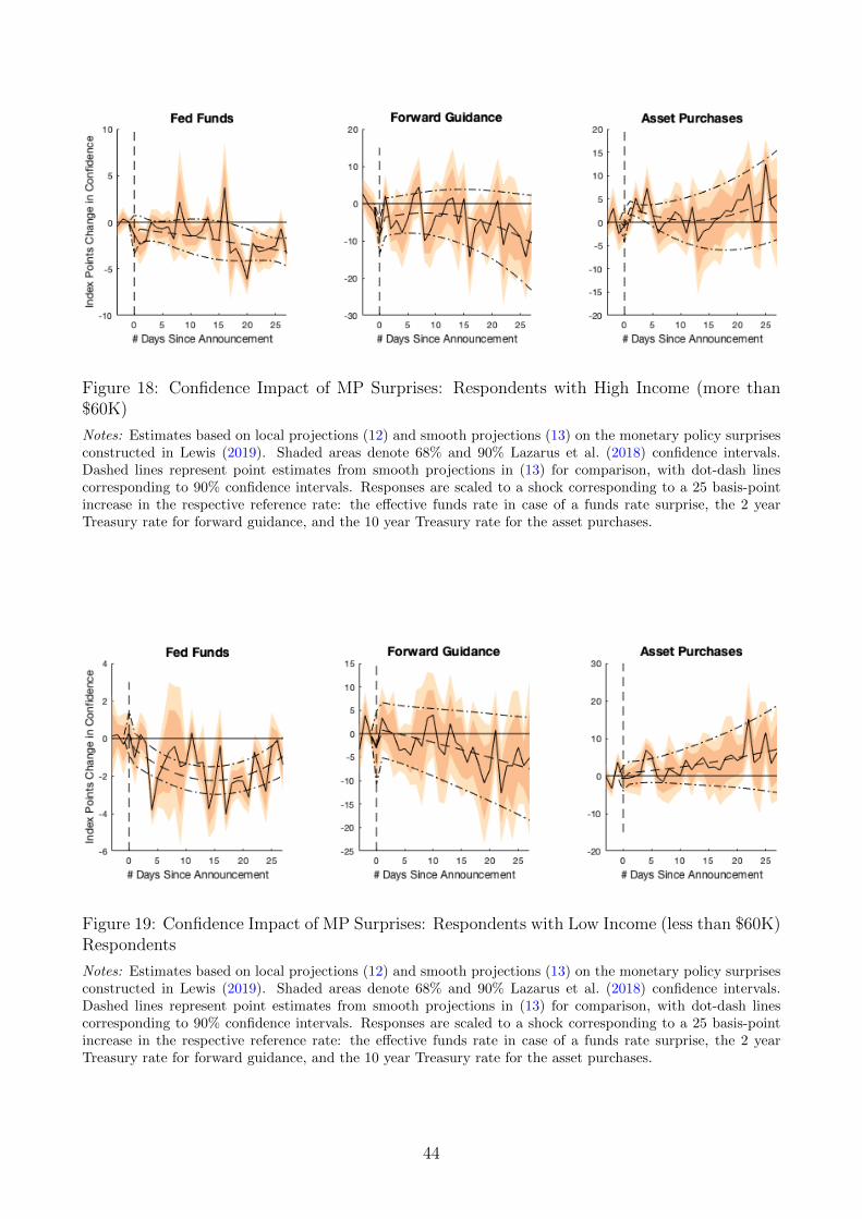
Figure 18: Confidence Impact of MP Surprises: Respondents with High Income (more than$60K)

Notes: Estimates based on local projections (12) and smooth projections (13) on the monetary policy surprisesconstructed in Lewis (2019). Shaded areas denote 68% and 90% Lazarus et al. (2018) confidence intervals.Dashed lines represent point estimates from smooth projections in (13) for comparison, with dot-dash linescorresponding to 90% confidence intervals. Responses are scaled to a shock corresponding to a 25 basis-pointincrease in the respective reference rate: the effective funds rate in case of a funds rate surprise, the 2 yearTreasury rate for forward guidance, and the 10 year Treasury rate for the asset purchases.

Figure 19: Confidence Impact of MP Surprises: Respondents with Low Income (less than $60K)Respondents

Notes: Estimates based on local projections (12) and smooth projections (13) on the monetary policy surprisesconstructed in Lewis (2019). Shaded areas denote 68% and 90% Lazarus et al. (2018) confidence intervals.Dashed lines represent point estimates from smooth projections in (13) for comparison, with dot-dash linescorresponding to 90% confidence intervals. Responses are scaled to a shock corresponding to a 25 basis-pointincrease in the respective reference rate: the effective funds rate in case of a funds rate surprise, the 2 yearTreasury rate for forward guidance, and the 10 year Treasury rate for the asset purchases.

44

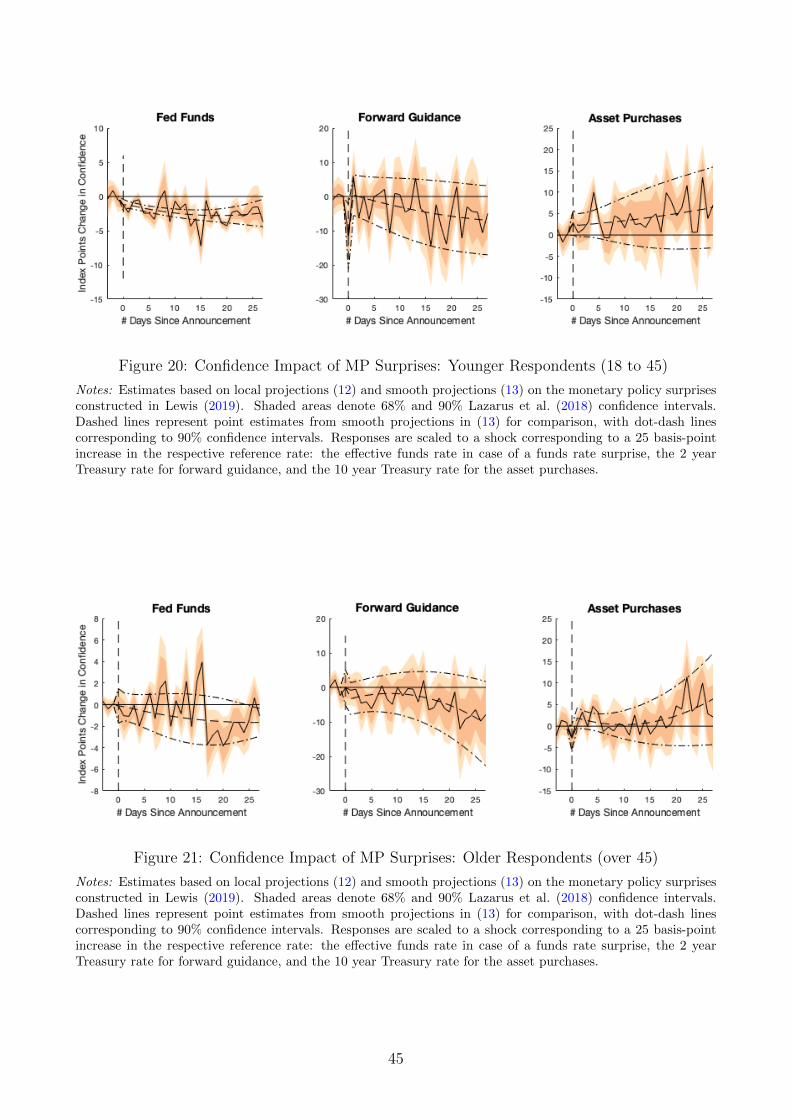
Figure 20: Confidence Impact of MP Surprises: Younger Respondents (18 to 45)

Notes: Estimates based on local projections (12) and smooth projections (13) on the monetary policy surprisesconstructed in Lewis (2019). Shaded areas denote 68% and 90% Lazarus et al. (2018) confidence intervals.Dashed lines represent point estimates from smooth projections in (13) for comparison, with dot-dash linescorresponding to 90% confidence intervals. Responses are scaled to a shock corresponding to a 25 basis-pointincrease in the respective reference rate: the effective funds rate in case of a funds rate surprise, the 2 yearTreasury rate for forward guidance, and the 10 year Treasury rate for the asset purchases.

Figure 21: Confidence Impact of MP Surprises: Older Respondents (over 45)

Notes: Estimates based on local projections (12) and smooth projections (13) on the monetary policy surprisesconstructed in Lewis (2019). Shaded areas denote 68% and 90% Lazarus et al. (2018) confidence intervals.Dashed lines represent point estimates from smooth projections in (13) for comparison, with dot-dash linescorresponding to 90% confidence intervals. Responses are scaled to a shock corresponding to a 25 basis-pointincrease in the respective reference rate: the effective funds rate in case of a funds rate surprise, the 2 yearTreasury rate for forward guidance, and the 10 year Treasury rate for the asset purchases.

45

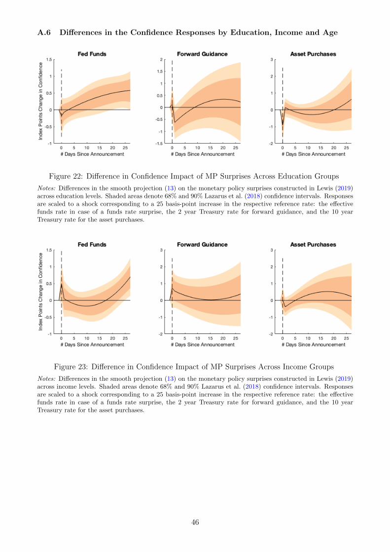
A.6 Differences in the Confidence Responses by Education, Income and Age

Figure 22: Difference in Confidence Impact of MP Surprises Across Education Groups

Notes: Differences in the smooth projection (13) on the monetary policy surprises constructed in Lewis (2019)across education levels. Shaded areas denote 68% and 90% Lazarus et al. (2018) confidence intervals. Responsesare scaled to a shock corresponding to a 25 basis-point increase in the respective reference rate: the effectivefunds rate in case of a funds rate surprise, the 2 year Treasury rate for forward guidance, and the 10 yearTreasury rate for the asset purchases.

Figure 23: Difference in Confidence Impact of MP Surprises Across Income Groups

Notes: Differences in the smooth projection (13) on the monetary policy surprises constructed in Lewis (2019)across income levels. Shaded areas denote 68% and 90% Lazarus et al. (2018) confidence intervals. Responsesare scaled to a shock corresponding to a 25 basis-point increase in the respective reference rate: the effectivefunds rate in case of a funds rate surprise, the 2 year Treasury rate for forward guidance, and the 10 yearTreasury rate for the asset purchases.

46

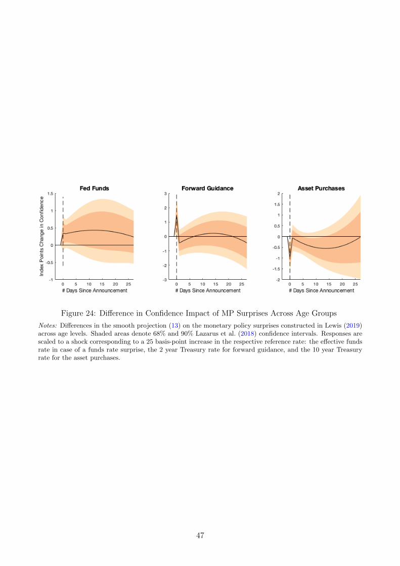
Figure 24: Difference in Confidence Impact of MP Surprises Across Age Groups

Notes: Differences in the smooth projection (13) on the monetary policy surprises constructed in Lewis (2019)across age levels. Shaded areas denote 68% and 90% Lazarus et al. (2018) confidence intervals. Responses arescaled to a shock corresponding to a 25 basis-point increase in the respective reference rate: the effective fundsrate in case of a funds rate surprise, the 2 year Treasury rate for forward guidance, and the 10 year Treasuryrate for the asset purchases.

47