do macroeconomic variables explain future stock market ... macroeconomic variables... ·...

Proceedings of the 2013 SAAA Biennial Conference

1067

MAF014

Do Macroeconomic Variables Explain Future

Stock Market Movements in South Africa?

Andrew MacFarlane, MCom *

and

Darron West, MCom MPhil CA(SA) CFA

Senior Lecturer, Department of Finance and Tax, University of Cape Town

E-mail: [email protected]

Contact address for the authors:

Department of Finance and Tax

University of Cape Town

Private Bag X3

Rondebosch

7701

mailto:[email protected]


1068

* Portions of this paper were submitted originally by this author in partial fulfilment of

the dissertation requirements for the degree of Master of Commerce in Financial and

Risk Management in the Faculty of Commerce at the University of Cape Town.


1069

Abstract

This study addresses the empirical question of whether macroeconomic variables drive

future stock market returns in South Africa. Where such a relationship can be found, the

macroeconomic variables are useful predictive information for future equity index

returns. Data was examined over the 45 year period from 1965 to 2010. The

macroeconomic variables were selected based on international and local precedent of

influential macroeconomic factors. Through the use of Johansen multivariate

cointegration, Granger causality and innovation accounting, it was found that the selected

South African macroeconomic variables do not significantly influence future FTSE/JSE

All Share Index returns.


1070

1. Introduction

Equity prices are generally expected to have a strong relationship with macroeconomic

variables. Economic factors affect the discount rates, companies‘ ability to generate cash

flows as well as future dividend payouts. Thus, the macroeconomic variables may

become key drivers of underlying company returns. These returns should then influence

the intrinsic stock price of the share and therefore an observable relationship should be

expected and subsequent causality should be found.

Previous studies, both internationally and locally have examined the relationship and

causality between macroeconomic variables and stock market returns in order to ascertain

whether current and future stock market returns are a function of macroeconomic

variables. If macroeconomic variables do constitute predictive information for future

stock market returns, it would be critical to take macroeconomic variables into account

when making investing decisions.

Johansen cointegration (Johansen 1991) and Granger causality analysis (Granger 1969)

are used in this study. These approaches have become standard empirical tests when

investigating long run relationships and the subsequent underlying causality. Innovation

accounting is used as an additional evaluation method in order to analyse the

interrelationships amongst the macroeconomic variables chosen. This is done through

examining the response of the stock exchange to a significant movement in the selected

macroeconomic variables.

This paper uses the approach described above to examine whether South African

macroeconomic factors have influenced the FTSE/Jse All Share Index (ALSI) returns

over the 45 years from 1965 to 2010, and further whether those macroeconomic variables

constitute future predictive information for the ALSI‘s future returns.


1071

This study avoids the potential inaccuracies set out by Su Zho (2001) by using a long

time horizons with a high number of observations and a short lag length between

observations when testing the data for causality and predictive ability.

This paper is structured in the following way. Section 2 sets out the hypothesised model

and the theoretical expected outcomes of the model. Section 3 briefly sets out the data

period and the resource used to acquire the data. The empirical methodology is outlined

in section 4. Section 5 tests the relationships empirically using cointegration, causal

analysis and innovation accounting. Section 6 concludes the study proposes possible

avenues for further analysis.


1072

2. Hypothesised model

According to Chen, Roll and Ross (1986), the selection of applicable macroeconomic

variables is based on their hypothesized effect on either the cash flows and/or the required

rate of return as per valuation models. This study draws on existing theory and empirical

evidence when deciding on which macroeconomic variables are appropriate to include in

the model.

The proxy for the level of real economy activity is GDP (Cheung and Ng (1998),

Wongabanpo and Sharma (2001), Chundri and Smiles (2004), Gan et al (2006), Hsing

(2011) and Jefferis and Okeahalam (2000)). South African GDP is only made public on a

quarterly basis. An increase in output may increase future expected cash flows and

subsequent profitability. Thus, it is initially expected that a positive relationship between

stock prices and GDP will exist and that GDP will have a causal effect on the ALSI.

It is hypothesised that there will be a negative relation between inflation and stock prices.

Inflation raises a firm‘s production costs and therefore decreases its future cash flow

which lowers revenue as well as profits. Inflation would also likely inform the tightening

of monetary policies which would have an adverse effect on profits (as financing costs

increase) and stock price (as discount rates increase). This study employs the Consumer

Price Index (CPI) as a measure of inflation. This is consistent with Mukherjee and Naka

(1995) , Maysami and Koh (2000), Nasseh and Strauss (2000), Wongbangpo and Sharma

(2001), Ibrahim and Aziz (2003), Gunsekaraage et al (2004), Gan et al (2006) and Humpe

and MacMillain (2009). Gupta and Modise (2011) and Van Rensburg (1995) investigated

this effect in South Africa.

Interest rates directly affect the discount rate in the discounted cash flow valuation model

and influence future cash flows. An increase in interest rates raises the required rate of

return, which in turn inversely affects the value of the asset. Additionally, the opportunity


1073

cost of holding low or no yield assets in a portfolio will increase and result in a

reallocation from equities to such higher yield, lower risk assets . Hence, there should be

an inverse relationship between the interest rate and stock prices. Interest rates are used in

similar studies by Bulmash and Trivoli (1991), Mukherjee and Naka (1995), Kwon and

Shin (1999), Karamustafa and Kucukkale (2003), Nasseh and Strauss (2000), Maysami

and Koh (2000), Gan et al (2006), Brahmasrene and Jiranyakul (2007) and Humpe and

MacMillain (2009). In South African studies, Jefferis and Okeahalam (2000), Alam and

Uddin (2009), Mangani (2008a), Jefferis and Okeahalam (2000) studied this effect.

The appreciation of the rand dollar exchange rate is hypothesised as being inversely

related to the stock price index. Conversely, the local currenciy‘s depreciation will

increase exports causing the competitiveness and subsequent profits of South African

listed companies resulting in higher stock market value. Internationally, the role of

exchange rates has been examined in studies by Mukherjee and Naka (1995), Kwon and

Shin (1999), Karamustafa and Kucukkale (2003), Maysami and Koh (2000),

Wongbangpo and Sharma (2001), Ibrahim and Aziz (2003), Gunsekaraage et al (2004),

Gan et al (2006) and Brahmasrene and Jiranyakul (2007). In South Africa, Hsing (2011),

Gupta and Modise (2011), Bonga-Bonga and Makakbule (2010) and Jefferis and

Okeahalam (2000) have examined this factor.

The role of money supply may have either a positive or negative effect on stock prices as

shown by Mukherjee and Naka (1995), Cheung and Ng (1998), Kwon and Shin (1999),

Maysami and Koh (2000), Wongbangpo and Sharma (2001), Karamustafa and Kucukkale

(2003), Ibrahim and Aziz (2003), Gunsekaraage et al (2004), Chaudhuri and Smiles

(2004), Gan et al (2006), Wong, Khan and Du (2006), Brahmasrene and Jiranyakul

(2007) and Humpe and MacMillain (2009). South African studies using money supply

have been by Hsing (2011) and Gupta and Modise (2011). The money supply may

increase owing to inflation and therefore may have a negative relationship with stock


1074

prices. However, the increase in money supply creates demand for equities (as interest

rates fall and returns are sought by investors) which results in increase in stock prices.


1075

3. Data

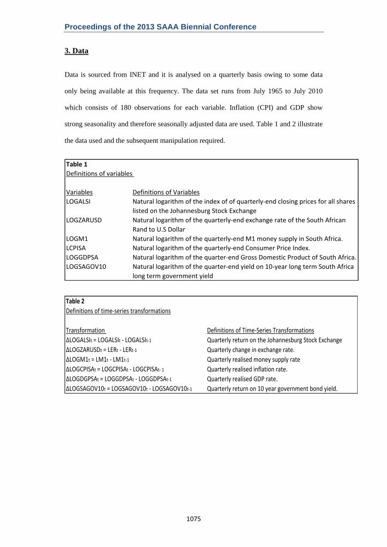
Data is sourced from INET and it is analysed on a quarterly basis owing to some data

only being available at this frequency. The data set runs from July 1965 to July 2010

which consists of 180 observations for each variable. Inflation (CPI) and GDP show

strong seasonality and therefore seasonally adjusted data are used. Table 1 and 2 illustrate

the data used and the subsequent manipulation required.

Table 1

Definitions of variables

Variables Definitions of Variables

LOGALSI Natural logarithm of the index of of quarterly-end closing prices for all shares

listed on the Johannesburg Stock Exchange

LOGZARUSD Natural logarithm of the quarterly-end exchange rate of the South African

Rand to U.S Dollar

LOGM1 Natural logarithm of the quarterly-end M1 money supply in South Africa.

LCPISA Natural logarithm of the quarterly-end Consumer Price Index.

LOGGDPSA Natural logarithm of the quarter-end Gross Domestic Product of South Africa.

LOGSAGOV10 Natural logarithm of the quarter-end yield on 10-year long term South Africa

long term government yield

Table 2

Definitions of time-series transformations

Transformation Definitions of Time-Series Transformations

∆LOGALSIt = LOGALSIt - LOGALSIt-1 Quarterly return on the Johannesburg Stock Exchange

∆LOGZARUSDt = LERt - LERt-1 Quarterly change in exchange rate.

∆LOGM1t = LM1t - LM1t-1 Quarterly realised money supply rate

∆LOGCPISAt = LOGCPISAt - LOGCPISAt- 1 Quarterly realised inflation rate.

∆LOGDGPSAt = LOGGDPSAt - LOGGDPSAt-1 Quarterly realised GDP rate.

∆LOGSAGOV10t = LOGSAGOV10t - LOGSAGOV10t-1 Quarterly return on 10 year government bond yield.


1076

4. Empirical Methodology

Cointegration analysis (Johansen, 1991) is used to determine the long term relationship

between macroeconomic variables and the stock market. Verbeek (2008) notes that

cointegration is a statistical property of a time series where variables are cointegrated if

they each share a common trend or they share a certain type of similarity in terms of their

long-term fluctuations; however they may not automatically move together and may be

otherwise unrelated.

According to Su Zhou (2001), defining long run relationships and subsequent

interpretations from cointegration depend on both of the length of time of the study as

well as the number of observations. Su Zhou‘s (2001) findings indicate that using a small

sample of 30 to 50 annual observations, instead of more observations of higher frequency

data, may not only result in significant loss of the test‘s power but also very likely

contribute to the problem of size distortion. The power of the cointegration test with a

small number of years and observations makes the results very sensitive to the lag length

used and the test is more easily affected by the problem of under-parameterization. This

paper therefore avoids these potential pitfalls by employing an extended number of years

as well as an adequate frequency with a low lag length when testing the data.

To apply standard testing procedures such as cointegration in a dynamic time series

model, it is normally required that the respective variables are stationary since most

econometric theory is built upon the assumption of stationarity (Verbeek, 2008).

Stationarity is defined by Challis and Kitney (1991) as a quality of process in which the

statistical parameters such as the mean, standard deviation autocorrelation etc do not

change with time and depends on the lag alone at which the function was calculated. This

is critical as without the normal distribution, the subsequent time series analysis will give

http://en.wikipedia.org/wiki/Statistical

http://en.wikipedia.org/wiki/Time_series


1077

incorrect results. When time series data does not follow the normal distribution due to

fluctuations, that data is non-stationary.

The non-stationarity of a series can influence its behaviour and properties substantially.

Verbeek (2008) stipulates that regressing a non-stationary variable upon another non-

stationary variable may lead to spurious regression.. Thus any correlation between two

such variables is misleading as it does not entail causation.

According to Joshi and Shukla (2009), when one is dealing with non-stationarity, the t-

ratios will not follow a t-distribution, so one cannot correctly test the regression

parameters. Secondly, if the series is consistently increasing over time, the sample mean

and variance will grow with the size of the sample, and they will always underestimate

the mean and variance in future periods. If the mean and variance of a series are not well-

defined then neither are its correlations with other variables. When testing time series

models, the implication that non-stationary variables can lead to spurious regressions

means that some form of testing of cointegration is almost mandatory (Harris, 1994).

However, the use of non-stationary variables does not necessarily result in invalid

estimators as an important exception arises when two or more variables are cointegrated.

If the non-stationary variables exist in a particular linear combination that is stationary

then a long run relationship between these variables exists (Verbeek, 2008).

The first step of the process of testing for long run relationships between variables

involves a test for stationarity and the order of the integration of the variables is

estimated. The Augmented Dickey-Fuller (ADF) and Phillips-Perron tests for unit roots

are used in order to do this.

Once the order of integration of each variable is determined, the next step is to calculate

the optimal lag length for the Vector Auto Regression (VAR) as all results in the VAR

model depend on the right model specification.


1078

As explained by Liew (2004), an auto regressive process with a lag length p refers to a

time series in which its current value is dependent on its first p lagged values. The

autoregressive lag length p is always unknown however, and therefore it has to be

estimated through a lag length selection criterion such as the Aikaike‘s information

criterion (AIC) (Akaike 1973) or Schwarz information criterion (SIC) (Schwarz 1978).

The importance of lag length determination criteria is shown by Braun and Mittnik

(1993) who illustrate that the approximation of a VAR whose lag length is contrary to

what the actual correct lag length should be leads to inaccurate results. Granger causality,

impulse response functions and variance decompositions that may be calculated from the

estimated VAR are similarly affected.

Additionally, Lütkepohl (1993) points out that selecting a higher order lag length than the

actual correct lag length causes an increase in the mean-squared forecast errors of the

VAR. Selecting a lower value lag length than the true lag length frequently generates

autocorrelated errors. Hafer and Sheehan (1989) also find that the accuracy of forecasts

from VAR models can vary considerably when using mis-specified lag lengths.

When using Johansen (1991) cointegration, Banerjee et al. (1998) propose that the

number of cointegrating vectors generated by the Johansen approach may be sensitive to

the number of lags in the VAR and therefore one needs to determine the optimal lag

length.

For this study, owing to the large sample size, the SIC is most appropriate owing to its

superior large sample properties (Myung, Tang and Pitt (2009), Azzem (2007), Burnham

and Anderson (2002) and Johnson and Scott (1999)).

4.1 Cointegration


1079

Once the appropriate lag length has been defined, the cointegration analysis is applied to

determine whether the time series of these variables displays a stationary process in a

linear combination.

Engle and Granger (1987) provide a means for testing for cointegration in a single

equation structure and the Johansen (1991) method enables testing for cointegration in a

system of equations. Although Engle and Granger‘s two step error correction model can

be used in multivariate context, the vector error correction model (VECM) gives more

efficient estimates of cointegrating vectors (Phillips, 1991).

The Johansen procedure is based on the VECM to test for at least one long run

relationship between the variables. This step is consistent with Mukherjee and Naka

(1995), Maysami and Koh (2000), Wongbangpo and Sharma (2001), Ibrahim and Aziz

(2003), Gunsekaraage et al (2004) and Humpe and McMillian (2007).

According to Maysami and Koh (2000), the VECM is a full information maximum

likelihood model which therefore permits the testing for cointegration in a whole system

of equations in one step and which does not require a specific variable to be normalized.

This means that it avoids carrying over the errors from the first step into the second and

gives more efficient estimators of cointegrating vectors, as would be the case if Engle and

Granger‘s methodology is used. It also has the advantage of not requiring a priori

assumptions of endogenity or exogenity of the variables.

The following Johansen multivariate model is used to calculate the relationships between

the variables;

∆Xt = Γ1∆Xt-1 + Γ2∆Xt-2 + ... + Γk-1∆Xt-k+1 + ∏Xt-k + µ + ФDt + єt

(1)


1080

where Γi = -I + ∏1 + ∏2 + ...+ ∏i for i = 1,2,k-1;

(2)

∏ = -I + ∏1 + ∏2 + ...+ ∏k I is an identity matrix

(3)

The matrix Γi comprises the short term adjustment parameters, and matrix ∏ contains the

long term equilibrium relationship information between the X variables. The ∏ could be

decomposed into the the product of two n by r matrix α and β so that ∏ = αβ where the β

matrix contains r cointegration vectors and α represents the speed of adjustment

parameters (Johansen (1998) and Gan et al. (2006)).

4.2 Granger Causality Test

Once the relationship between the two has been established, the next objective of this

study is to observe whether the macroeconomic variables selected are valuable in

predicting future stock market movements in South Africa. Granger causality is a test

used to determine whether one time series can forecast another. Roebroeck et al. (2005)

describe Granger causality as quantifying the usefulness of unique information in one

time series in predicting values of the other. Specifically, if incorporating past values of x

improves the prediction of the current value of y, then x Granger causes y. Therefore,

precedence is used to identify the direction of causality from information in the data.

Roebroek et al. (2005) explain that the VAR model can be thought of as a linear

prediction model that forecasts the current value based on a linear combination of the

most recent past influential variables. Thus, the current value of a component is predicted

based on a linear combination of its own past values and past values of other components.

This shows the value of the VAR model in quantifying Granger causality between groups

of components.


1081

The practicability of the Granger causality test depends on the stationarity of the system.

If the series is stationary, the null hypothesis of no Granger causality can be tested by the

standard Wald tests as shown by Lutkepohl (1991). Additionally, because Granger

causality requires large sample sizes to make conclusions, it should evaluated over a long

time period.The Gan et al. (2006) illustration of Granger causality is used to test the lead-

lag relationship between the macroeconomic variables and the ALSI thus:

k k

∆Xt = ax + ∑ βx,i ∆Xt-i + ∑ ωx,i∆Yt-i + φxECTx,t-i + єx,t

(4)

i=1 i=1

k k

∆Yt = ax + ∑ βy,i ∆Xt-i + ∑ ωy,i∆Xt-i + φyECTx,t-i + єy,t

(5)

i=1 i=1

where φx and φy are the parameters of the ECT term, measuring the error correction

mechanism that drives the Xt and Yt back to their long run equilibrium relationship.

Furthermore, Gan et al. (2006) stipulate that the null hypothesis for (4) is H0: ∑ ωx, = 0

which suggests that the lagged terms ∆Y do not belong to the regression. Conversely, the

null hypothesis for the equation (5) is H0 : ∑ ωy, = 0 which implies that the lagged terms

∆X do not belong to the regression.

4.3 Innovation Accounting

Innovation accounting such as the impulse response function and variance decomposition

is used in analysing the interrelationships among the variables chosen in the system (Gan

et al, 2006). Accordingly, this study proceeds to evaluate variance decompositions and


1082

impulse-response functions based on the VAR specification to capture the dynamic

interactions among the variables (Wongbangpo and Sharma (2001), Ibrahim and Aziz

(2003), Nasseh and Strauss (2000), Chundri and Smiles (2004), Gunsekaraage et al

(2004) and Gan et al. (2006)).

4.3.1 Impulse response functions

A shock to the i-th variable not only directly affects the i-th variable but it is also

transmitted to all of the other endogenous variables through the dynamic lag structure of

the VAR. An impulse response function traces the effect of a one time shock function to

one of the innovations on current and future values of the endogenous variables.

Therefore, the impulse response describes the ALSI‘s reaction to a shock in the

macroeconomic variables and the subsequent periods.

If the innovations et are contemporaneously uncorrelated, interpretation of the impulse

response is as follows (Shachmurove and Shachmurove., 2008): The i-th innovation ei,t is

simply a shock to the i-th endogenous variable yi,t. However, innovations are generally

correlated, and may be viewed as having a common component which cannot be

associated with a specific variable. In order to interpret the impulses, it is common to

apply a transformation P to the innovations so that they become uncorrelated with the

formula being

vt = P et ~ (o, D),

where D is a diagonal covariance matrix.

4.3.2 Variance decompositions

The impulse response function trails the effect of a shock to one variable on the other

variables in the VAR. The variance decomposition, however, separates the variation in

one the South African macroeconomic variables into the constituent shocks to the VAR.


1083

Variance decomposition shows how much of the forecast error variance for any variable

in the VAR is explained by innovations to each explanatory variable over a series of time

horizons.

Variance decompositions are constructed from a VAR with orthogonal residuals and

hence can directly address the contribution of macroeconomic variables in forecasting the

variance of stock prices (Sims, 1980). Cointegration implies that R-squared approaches 1

and therefore the variance decomposition in levels approximates the total variance of

stock prices.

Enders (1995) states the proportion of Y variance due to Z shock can be expressed as:

∂22 [ a12(0)

2 + a12(1)

2 + …… + a12(m-1)

2]

∂y (m)2

Per Enders (1995) and Gan et al. (2006) one can see that as m period increases the ∂y(m)2

also increases. Furthermore, this variance can be separated into two series: yt and zt

series. Consequently, the error variance for y can be composed of eyt and ezt. If eyt

approaches unity it implies that yt series is independent of zt series. It can be said that yt is

exogenous relative to zt. On the other hand, if eyt approaches zero (indicates that ezt

approaches unity) the yt is said to be endogenous with respect to the zt (Gan et al., 2006).


1084

5. Empirical Results

5.1 Cointegration Analysis

Cointegration requires the variables to be integrated to the same order and therefore the

Augmented Dickey-Fuller (ADF) and Phillips-Peron tests are used. The results of the

tests are given in Table 3. Both ADF and Phillip-Perron do not reject the null hypothesis

of the existence of a unit root in log levels of all variables. Hence the presence of non-

stationarity is indicated which may lead to spurious relationships.

However, the tests do reject the same null hypothesis in the log first difference of the

series. This indicates that GDP, inflation (CPI), money supply, rand dollar exchange rate

and the interest rate (10 year government bond yield) are integrated of order one. Since

the various variables exhibit stationarity the analysis may continue.

Table 3

Augmented Dickey-Fuller Test Results

Null Hypothesis: LOGCPISA has a unit root Null Hypothesis: LOGGDPSA has a unit root

t-Statistic Prob.* t-Statistic Prob.*

Augmented Dickey-Fuller test -1.28439 0.6365 Augmented Dickey-Fuller test -1.1628 0.6901

First Differenced First Differenced


Augmented Dickey-Fuller test -3.50302 0.009 Augmented Dickey-Fuller test -4.99569 0

Null Hypothesis: LOGM1 has a unit root Null Hypothesis: LOGSAGOV10 has a unit root


Augmented Dickey-Fuller test 0.338204 0.9797 Augmented Dickey-Fuller test -1.87944 0.3414

First Differenced First Differenced


Augmented Dickey-Fuller test -14.0106 0 Augmented Dickey-Fuller test -11.5893 0

Null Hypothesis: LOGZARUSD has a unit root

t-Statistic Prob.*

Augmented Dickey-Fuller test -0.24608 0.9288

First Differenced

t-Statistic Prob.* *MacKinnon (1996) one-sided p-values.

Augmented Dickey-Fuller test statistic-12.0026 0


1085

Before testing the VAR for cointegration, the lag length criterion needs to be specified.

The optimum lag length suggested by SIC was 1.

In selecting the lag length, a requirement is that the error terms for the equations must be

uncorrelated. The Ljung-Box-Pierce Q statistic tests the null hypothesis that the error

terms are uncorrelated. The results indicate the lack of autocorrelation in the residuals and

therefore the model is adequately specified.

The results of Johansen cointegration test are reported in Table 4. There are 3

cointegrating equations at the 5% level of significance.

Johansen and Juselius (1990) note that the first cointegrating vector that corresponds to

the largest eigenvalue is the most correlated with the stationary part of the model and

therefore will be its most useful. Hence, in this long run study, the analysis is based on

the first cointegrating vector.

Table 4

Sample (adjusted): 1965Q4 2010Q2

Included observations: 179 after adjustments

Trend assumption: Linear deterministic trend

Series: LOGALSI LOGCPISA LOGGDPSA LOGM1 LOGSAGOV10 LOGZARUSD

Lags interval (in first differences): 1 to 1

Unrestricted Cointegration Rank Test (Trace)

Hypothesized

No. of CE(s) Eigenvalue Trace Statistic 0.05 Critical Value Prob.**

None * 0.407646 181.2234 95.75366 0

At most 1 * 0.192776 87.48980 69.81889 0.001

At most 2 * 0.135510 49.15625 47.85613 0.0375

At most 3 0.079733 23.09320 29.79707 0.2415

At most 4 0.041139 8.219767 15.49471 0.4422

At most 5 0.003904 0.700160 3.841466 0.4027

Trace test indicates 3 cointegrating eqn(s) at the 0.05 level

* denotes rejection of the hypothesis at the 0.05 level

**MacKinnon-Haug-Michelis (1999) p-values


1086

After normalising the coefficients of the ALSI to one in order to establish the long run

relationship of the variables against the ALSI from 1965-2010, the relationship can be

expressed as

ALSI = -7.548GDP + 0.322CPI + 2.452M1 – 2.433SAGB10 - 1.140ZARUSD

These estimated long run coefficients of the macroeconomic factors may be interpreted as

elasticity measures since the variables are expressed in natural logarithms. From these

results, one is able to interpret the long term relationship for the past 45 years and offer

possible theoretical explanations for the relationship, but not the causality, between the

ALSI and the macroeconomic variables.

5.2 Causal Analysis

When dealing with a cointegrated set of variables, Granger (1988) recommends that the

causal relations between the variable should be investigated within the structure of the

VECM. The lag value (SIC = 1) was tested against the 179 observations for each

variable. Two statistical tests are performed: the pairwise Granger Causality test and the

Block Exogeneity Wald test.

The pairwise Granger Causality test is used to identify the exogeneity of each variable

introduced in the system. The p values indicate the significance of lagged coefficients of

each variable in the equation of each endogenous variable.

The Block Exogeneity Wald Test is used to test the joint significance of each of the other

lagged endogenous variables in each equation and also to test for the joint significance of

all the other lagged endogenous variables in each equation. The causal test statistics are

shown in Table 5 below.


1087

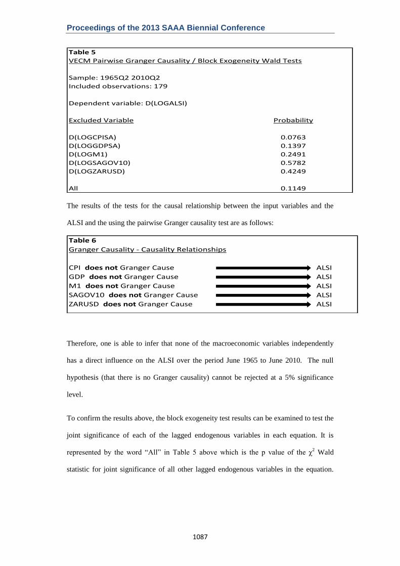
The results of the tests for the causal relationship between the input variables and the

ALSI and the using the pairwise Granger causality test are as follows:

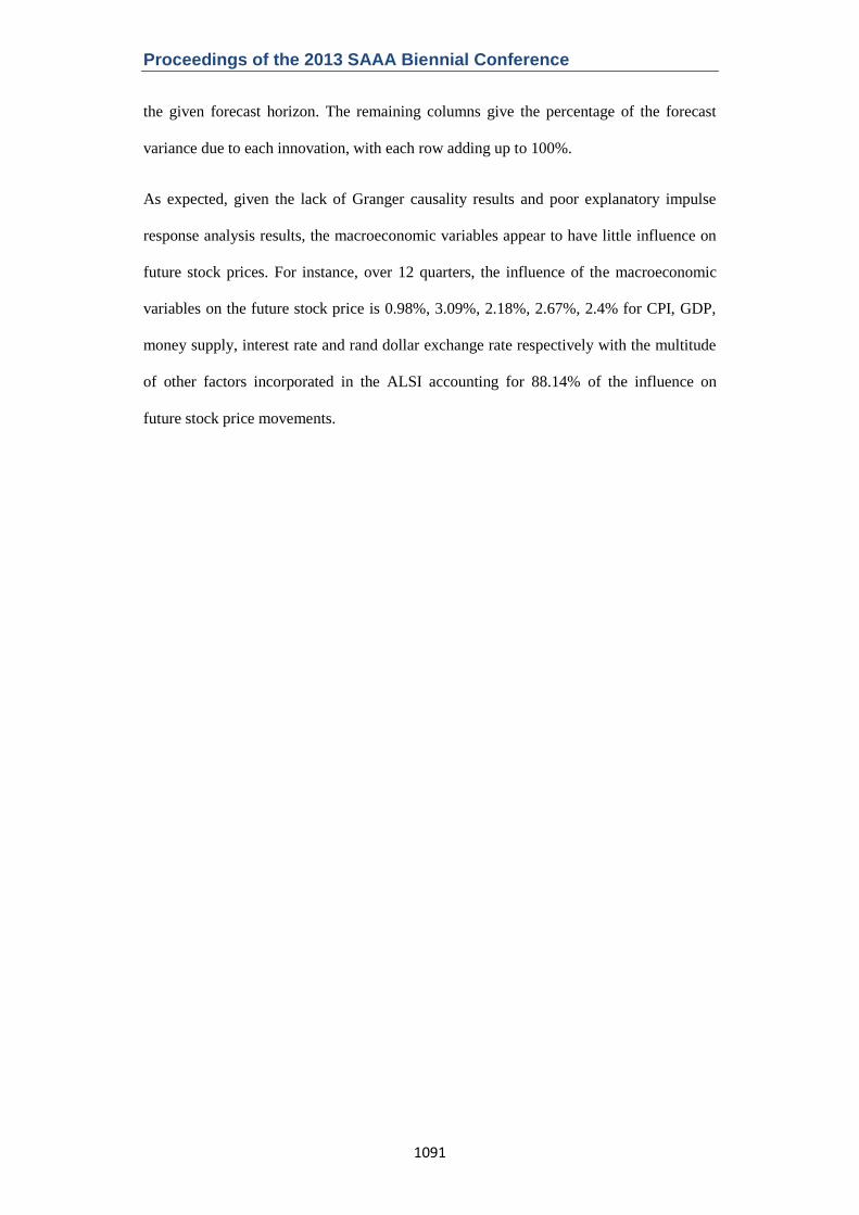
Therefore, one is able to infer that none of the macroeconomic variables independently

has a direct influence on the ALSI over the period June 1965 to June 2010. The null

hypothesis (that there is no Granger causality) cannot be rejected at a 5% significance

level.

To confirm the results above, the block exogeneity test results can be examined to test the

joint significance of each of the lagged endogenous variables in each equation. It is

represented by the word ―All‖ in Table 5 above which is the p value of the χ2 Wald

statistic for joint significance of all other lagged endogenous variables in the equation.

Table 5

VECM Pairwise Granger Causality / Block Exogeneity Wald Tests

Sample: 1965Q2 2010Q2

Included observations: 179

Dependent variable: D(LOGALSI)

Excluded Variable Probability

D(LOGCPISA) 0.0763

D(LOGGDPSA) 0.1397

D(LOGM1) 0.2491

D(LOGSAGOV10) 0.5782

D(LOGZARUSD) 0.4249

All 0.1149

Table 6

Granger Causality - Causality Relationships

CPI does not Granger Cause ALSI

GDP does not Granger Cause ALSI

M1 does not Granger Cause ALSI

SAGOV10 does not Granger Cause ALSI

ZARUSD does not Granger Cause ALSI


1088

Similarly, this test fails to reject the null hypothesis as the p-value of the causality is

insignificant at the 5% level

It can therefore be concluded that none of the macroeconomic variables has significant

Granger causality for the ALSI. This implies that in South Africa the value of the ALSI is

not a function of the past and current macroeconomic factors set out in this paper and that

these variables do not constitute useful predictive information for the ALSI‘s future

returns.

5.3 Innovation Accounting

5.3.1 Impulse Response Function

An impulse response function traces the effect of a one time shock function to one of the

innovations on current and future values of the endogenous variables. Therefore, the

impulse response describes the ALSI‘s reaction as a function of time to the

macroeconomic factors at the time of the shock and the subsequent points. The results of

the impulse response analysis of the South African macroeconomic variables and the

ALSI is shown below:

The forecast period is the first column and is the period of time forecasted ahead (viz. bi-

annually, annually, 3 years and 5 years respectively). As expected, given the lack of

causality, a one standard deviation shock in any of the macroeconomic variables has an

Table 7

Impulse Resonse analysis

Response of stock prices (to one standard deviation shock in macroeconomic variables)

Periods ahead LOGCPI LOGGDP LOGM1 LOGSAGOV10 LOGZARUSD

2 0.002313 0.004117 -0.005798 -0.005527 0.004252

4 0.005572 0.010032 -0.012373 -0.012211 0.010522

12 0.009288 0.016122 -0.00699 -0.010302 0.013721

20 0.010047 0.016549 0.001435 -0.001084 0.005543


1089

inconsequential effect on the ALSI. For example, the response of the ALSI two quarters

or 6 months after one standard deviation shock in the macroeconomic variable is 0.2%,

0.4%, -0.5%, -0.5% and 0.4% for CPI, GDP, money supply, interest rate and rand dollar

exchange rate respectively.


1090

5.3.2 Variance Decomposition

The impulse response function trails the effect of a shock to one variable on the other

variables in the VAR. The variance decomposition, however, separates the variation of

the South African macroeconomic variables into the constituent shocks to the VAR.

Ordering of the variables is of importance given the causal influence that they may have

on the relevant stock index. However, given that the South African macroeconomic

variables and the ALSI have been shown to have a non causal relationship, the ordering

becomes less important.

According to Sims (1980), the power of the Granger causality can be ascertained by the

variance decomposition. In the South African example, it would be expected that owing

to the lack of Granger causality between the macroeconomic variables and the ALSI,

there would be a very small portion of a variable (such as the money supply) that would

explain the forecast error variance of the ALSI. The decomposition between the ALSI

and South African macroeconomic variables is shown below.

The variance decomposition analysis should compare favourably with the impulse

response analysis. The table format shows separate variance decompositions for each

endogenous variable. The ―S.E‖ in the second column is the forecast error of the ALSI at

Table 8

Variance Decomposition analysis

Forecast error variance of stock prices (explained by innovations in the macroeconomic variables)

Periods ahead S.E. LOGALSI LOGCPI LOGGDP LOGM1 LOGSAGOV10 LOGZARUSD

2 0.155739 99.56896 0.022063 0.069866 0.138617 0.125966 0.074528

4 0.199324 97.5621 0.134847 0.434861 0.712914 0.679844 0.475437

12 0.252154 88.13933 0.978001 3.091362 2.183362 2.669988 2.39796

20 0.263911 83.64311 1.276507 5.829448 2.076281 2.778053 3.705661


1091

the given forecast horizon. The remaining columns give the percentage of the forecast

variance due to each innovation, with each row adding up to 100%.

As expected, given the lack of Granger causality results and poor explanatory impulse

response analysis results, the macroeconomic variables appear to have little influence on

future stock prices. For instance, over 12 quarters, the influence of the macroeconomic

variables on the future stock price is 0.98%, 3.09%, 2.18%, 2.67%, 2.4% for CPI, GDP,

money supply, interest rate and rand dollar exchange rate respectively with the multitude

of other factors incorporated in the ALSI accounting for 88.14% of the influence on

future stock price movements.


1092

6. Conclusion

Using both the Augmented Dickey-Fuller and Phillips Peron tests, it was found that the

macroeconomic variables are integrated of order one and therefore the data is stationary.

Cointegration was subsequently discovered amongst the variables revealing that there is a

long term relationship between the South African stock market and the macroeconomic

variables.

According the VECM model estimated in the study, inflation and money supply have a

positive relationship with the ALSI over the long run. However, inflation is not

significant. A negative relationship was found for the South African 10 year Government

Bond Yield (which is used as a measure of the interest rate), the rand dollar exchange rate

and GDP.

The influence of the macroeconomic factors influence on stock market returns was

examined. The Granger causality results indicated that the ALSI is not a function of the

past and current macroeconomic factors analysed in this paper and that these variables do

not constitute useful predictive information for the ALSI.

This assessment was then vindicated by use of innovation accounting. Impulse response

function traced the effect of a one standard deviation shock of the macroeconomic

variables on the South African stock exchange. The results were inconsequential.

Similarly, variance decomposition was used to explain the forecast error variance of the

ALSI for each individual macroeconomic variable with the results confirming the

previous findings of this study that the macroeconomic variables explain an insignificant

portion of future returns.


1093

Bibliography

Abdalla, I. S. & Murinde, V. (1997), ―Exchange Rate and Stock Price interactions in

emerging financial markets: Evidence on India, Korea, Pakistan and Philippines‖,

Applied Financial Economics, 7, 25-35.

Ahmed, S. (2008), ―Aggregate Economic Variables and Stock Markets in India‖,

International Research Journal of Finance and Economics, 14, 141-163

Ajayi, R. A. & Mougou, M. (1996), ―The dynamic relation between stock prices and

exchange rates‖, The Journal of Financial Research, Vol. 19, 193 - 207.

Akaike, H. (1973), ―Information theory and an extension of the maximum likelihood

principle‖, 2nd International Symposium on Information Theory by B. N. Petrov and F.

Csaki, eds., Akademiai Kiado: Budapest.

Akintoy, I. (2008), ―Efficient market Hypothesis and Behavioural Fiannce: A Review of

Literature‖, European Jouranl of Social Sciences, Volume 7, No. 2

Al-Khazali, O. and Pyun, C.S, (2004), ―Stock Prices and Inflation: New Evidence from

the Pacific-Basin Countries‖, Review of Quantitative Finance and Accounting, 22, 123-

140

Alam, M. and Uddin, G (2009), ― Relationship between Interest Rate and Stock Price:

Empirical Evidence from Developed and Developing Countries‖, International Journal of

Business and Managgement, Vol. 4, 43-51


1094

Alatiqi, S. and Fazel, S. (2008), ―Can Money Supply Predict Stock Prices?‖, Journal for

Economic Educators, 8(2), 54-59

Anari, A. and Kolari, J. (2001), ―Stock Prices and Inflation‖, Journal of Financial

Research, 24, 587-602

Appiah-Kusi, J. and Menyah, K. (2003) ―Return predictability in African stock markets‖

Review of Financial Economics, Volume 12, Issue 3, 247-270

Aron, J. Elbadawi, I. and Kahn, B. (2000), ―Real and Monetary Determinants of the Real

Exchange Rate in South Africa‖, Development issues in South Africa, ed. by Ibrahim

Elbadawi and Trudi Hartzendber (London: MacMillian)

Aron, J. and J. Muellbauer. (2002), ―Interest rate effects on output: evidence from a GDP

forecasting model for South Africa.‖ IMF Staff Papers 49, 185 - 213.

Azarmi, T., Lazar, D. and Jeyapaul, J. (2005), ―Is The Indian Stock Market A Casino?‖,

Journal of Business & Economics Research, 3,4

Bahmani-Oskooee, M., and A. Sohrabiab (1992), ―Stock prices and the effective

exchange rate of the dollar‖, Applied Economics, Vol. 24, 459-464.

Balassa, B. (1964), ―The Purchasing-Power Parity Doctrin: A Reappraisal‖, Journal of

Political Economy, Vol. 72, 584 - 96


1095

Banerjee, A . , Dolado, J. J . , Mestre, R., (1998), ―Error correction mechanism tests for

cointegration in a single equation framework‖, Journal of Time Series Analysis, 19,3,

267-284

Barberis, N., Shleifer, A. and Vishny, R. A. (1998) ―A model of investor sentiment‖,

Journal of Financial Economics, Vol. 49 307–343.

Bernake, B.S. and Gertler, M. (1999), ―Monetary Policy and Asset Price Volatility‖,

Federal

Reserve Bank of Kansas City, Economic Review, Fourth Quarter.

Bernanke, Ben S., and Alan S. Blinder (1992). "The Federal Funds Rate and the Channels

of Monetary Transmission." American Economic Review 82, 901-921.

Bernstein, W. and Arnott,R., (2003),― Earnings growth: the two percent dilution‖,

Financial Analyst Journal, September/October, 47 – 55

Bethlehem, G. 1972, ―An investigation of the return on ordinary share [sic] quoted on

The Johannesburg Stock Exchange with reference to hedging against inflation‖, The

South African Journal of Economics, vol. 40, no. 3, pp. 254 - 67.

Bhattacharya, B. and Mukherjee, J. (2003), ―Causal Relationship between Stock Market

and Exchange Rate. Foreign Exchange Reserves and Value of Trade Balance: A Case

Study for

India. Paper presented at the Fifth Annual Conference on Money and Finance in the

Indian

Economy, January 2003.


1096

Bhide, A., (1993), ―The hidden costs of stock market liquidity‖, Journal of Financial

Economics, Vol. 34, No.1, 31-51

Black, A., Fraser P. and MacDonald R., (1997), ―Business Conditions and Speculative

Assets‖, Manchester School, 1997, 4, 379-393.

Bhattacharya, B. & Mukherjee, J. (2003). ―Causal Relationship Between Stock Market

and Exchange Rate. Foreign Exchange Reserves and Value of Trade Balance: A Case

Study for India‖, Paper presented at the Fifth Annual Conference on Money and Finance

in the Indian Economy, January 2003.

Bodie, Z. (1976), ―Common stocks as a Hedge Against Inflation‖, Journal of Finance,

459-470

Boudoukh, J. and Richardson M., (1993), ―Stock retums and infiation: A long-horizon

perspective‖,

Economic Review, 83, 1346-55

Brahmasrene, T., & Jiranyakul, K. (2007), ―Cointegration and Causality between stock

index and

macroeconomic variables in an emerging market‖, Academy of Accounting and Financial

Studies Journal, 11(3), 17-30.

Braun, P. A. and S. Mittnik (1993), ―Misspecifications in Vector Autoregressions and

Their Effects on Impulse Responses and Variance Decompositions‖, Journal of

Econometrics, 59, 319-41.


1097

Bulmash, S. and Trivoli, G. (1991), ―Time lagged interactions between stock prices and

selected economic variables‖, The Journal of Portfolio Management, Summer, 61-67.

Carter, M. and May, J. (2001), ―One Kind of Freedom: Poverty Dynamics in Post-

Apartheid South Africa‖, World Development, Volume 29, Issue 12, 1987-2006

Challis, R. E., and Kitney, R. I., (1991), "Biomedical signal processing (in four parts).

Part 1 Time-domain methods", Medical & Biological Engineering & Computing, 28, 509-

524

Chaudhuri, K. and S. Smile, (2004), ―Stock market and aggregate economic activity:

evidence from Australia‖, Applied Financial Economics, 14, 121-129.

Chen, N. F, Roll, R., &. Ross, S. (1986), ‖Economic forces and the stock market‖,

Journal of Business 59(3)‖, 383–403.

Cheung, Y. and L. Ng (1998), ―International evidence on the stock market and aggregate

economic activity‖, Journal of Empirical Finance, 5, 281-296.

Chiang, T.C., Nelling, E., and Tan, L. (2008), ―The speed of adjustment to information:

evidence from the Chinese stock market‖, International Review of Economics and

Finance 17, 216-229.

Collins, D. and Abrahamson, M. (2004), ―African Equity Markets and the Process of

Financial

Integration‖, South African Journal of Economics, Vol. 72, No.4, 658-683.


1098

Collins, D. and Biekpe, N (2003), ―Contagion and Interdependence in African stock

markets‖, South Africa Journal of Economics, Vol. 71 No.1, 181—194.

Daniel, K. D., Hirshleifer, D. and Subrahmanyam, A. (1998), ―Investor psychology and

security market under and over-reactions‖, Journal of Finance, Vol. 53, 1839–1886.

Daniel, K. D., Hirshleifer, D. and Subrahmanyam, A. (2001), ―Overconfidence, arbitrage

and equilibrium asset pricing‖, Journal of Finance, Vol. 56, 2001, 921–65.

De Beer, J and Keyser, N, ―JSE returns, political developments and economic forces: A

historical perspective‖ Conference of the Economic History Society of South Africa

presentation

De Bondt, W. F.M., Shefrin, H., Muradoglu, G. and Staikouras, S.,(2008) ―Behavioural

Finance: Quo Vadis?‖ Journal of Applied Finance, Vol. 19, 7 - 21

De Bondt, W.F.M. and Thaler, R.H. (1985). ―Does the Stock Market Overreact?‖ Journal

of Finance, Vol. 15 No.3, 793-805.

De Kock Commission, (1984), ―The Monetary System and Monetary Policy in South

Africa.‖, Final Report of the Commission of Inquiry into the Monetary System and

Monetary Policy in South Africa, Government Printer.

Devereux, M.B and G.W. Smith, (1994), ―International risk sharing and economic

growth‖, International Economic Review, Vol. 35, No.3, 535-550.


1099

Dimson, E., Marsh P., and Staunton M., (2002), ―Triumph of the Optimists: 101 Years of

Global

Investment Returns‖, Princeton University Press, Princeton

Dimson, E., Marsh P., and Staunton M. (2010), ―Economic growth‖, Credit Suisse Global

Investment Returns Yearbook, 12-19

Dornbusch, R., (1987), ―Exchange Rate Economics: 1986‖, The Economic Journal, Vol.

97, pp. 1-18.

Dornbusch, R. & Fisher, S. (1980), ―Exchange rates and the current account‖. American

Economic Review, 70, 960-971.

Enders, W. and Dibooglu, S., (2001), ―Long-Run Purchasing Power Parity with

Asymmetric

Adjustment‖, Southern Economic Journal, Vol.68, No. 2, pp. 433-445.

Enders, W., (1995) ―Applied Econometric Time Series‖, John Wiley & Sons Inc., United

States

Engle, R. E., and Granger, C. (1987), ―Cointegration and error-correction: representation,

estimation and testing‖, Econometrica 55, 251–276.

Ehrmann, M. and Fratzscher, M. (2004), ―Taking Stock: Monetary Policy Transmission

to Equity Markets‖, Journal of Money, Credit and Banking, Vol 36, No.4, 719-737

Errunza, V. and Hogan, K. (1998), ―Macroeconomic determinants of European stock

market volatility‟, European Financial Management, Vol. 4, No. 3, 361–377


1100

Fama, E. F. (1981), ―Stock returns, real activity, inflation and money‖, The American

Economic Review 71, 545–565.

Fama, E. and French, K.R., (1989), ―Business conditions and expected returns on stocks

and bonds‖, Journal of Financial Economics, 25, 23-49.

Fama, E. F. (1990), ―Stock returns, expected returns and real activity‖, Journal of Finance

45, 1089–1108.

Ferson, W. and Harvey, C., (1991), ―The variation of economic risk premiums‖, Journal

of Political Economy, 99, 385-415.

Fisher, I., (1930), ―The Theory of Interest‖, (Macmillan, New York).

Flannery, M. J. and Protopapadakis, A. (2002), ―Macroeconomic Factors do Influence

Aggregate Stock Returns‖, Review of Financial Studies, 15, 751-782.

Friedman, M. (1956), ―The Quantity Theory of Money – A Restatement‖, Studies in

Quantity Theory of Money, Chicago

Frier and McLeod (1999), ―Equities, bonds,cash and inflation: Historical performance in

South Africa 1925 to 1998), Investment Analysts Journal, No. 50, 7-28

Frimpon. S, (2011), ―Speed of Adjustment of Stock Prices to Macroeconomic

Information: Evidence from Ghanaian Stock Exchange (GSE)‖, International Business

and Management, Vol.2, No. 1, 1-6


1101

Fung H. G., & Lie, C. J. (1990), ―Stock market and economic activities: a causal

analysis‖, in S.G Khee & R. P. Chang (Eds.) Pacific-Basin Capital Markets Research,

Amsterdam, North Holland

Gaffney, JV 2009, ―Value versus glamour investing: a South African case‖, MBA

dissertation, University of Pretoria, Pretoria, viewed 13/03/2011

<http://upetd.up.ac.za/thesis/available/etd-04082010-112808/ >

Gan, C., Lee, M., Young, H.W.A. and Zhang, J., (2006), ―Macroeconomic Variables and

Stock Market Interaction: New Zealand Evidence‖, Investment Management and

Financial Innovations, Volume 3, Issue 4, 89-101

Geske, R. and Roll R., (1983), ―The fiscal and monetary linkages between stock returns

and inflation‖, Joumal of Finance 3S, 1-33.

Graham, M. and Uliana, E. (2001), ―Evidence of a value growth phenomenon on the

Johannesburg Stock Exchange‖. Investment Analysts Journal, Vol. 53, 7-18.

Granger, C.W.J., 1969. "Investigating causal relations by econometric models and cross-

spectral methods". Econometrica Vol. 37 No.3, 424–438.

Granger, C., (1986), ―Developments in the study of cointegrated economic variables‖,

Oxford Bulletin of Economics and Statistics, 48, 213-228.

Granger, C., (1987), ―Co-Integration and Error Correction: Representation, Estimation,

and Testing‖, Econometrica, 55, 251-276.

Granger, C. (1988), ―Some recent development in a concept of causality‖, Journal of

Econometrics, 39, 199-211


1102

Griffin, J. Ji, X and Martin, J. (2003), ―Momentum Investing and Business Cycle Risk:

Evidence from Pole to Pole‖, The Journal of Finance, Vol. LVIII, No. 6

Gunasekarage, A., Pisedtasalasai, A. and Power, D.M. (2004), ―Macroeconomic

influence on the stock market evidence from an emerging market in South Asia‖, Journal

of Emerging Market Finance, Vol. 3, 285-304.

Gupta R., Modise, M.P. (2011), Macroeconomic Variables and South African Stock

Return

Predictability. working paper.

Cassel, G (1918), "Abnormal Deviations in International Exchanges," Economic Journal,

December, 413-415

Hafer, R. W. and R. G. Sheehan (1989), ―The Sensitivity of VAR Forecasts to Alternative

Lag

Structures‖, International Journal of Forecasting, 5, 399-408.

Hess, P. and Lee, B., (1999), ―Stock Returns and Inflation with Supply and Demand

Disturbances.‖ Review of Financial Studies 12, 1203–1218

Hong, H. and Stein, J. C. (1999), ‗A unified theory of underreaction, momentum trading

and overreaction in asset markets‘, Journal of Finance, Vol. 54, 1999, 2143–84.

Hong, H., Kubik, J. and Stein, J. C. (2005), ‗Thy neighbor‘s portfolio: Word-of-mouth

effects in the holdings and trades of money managers‘, Journal of Finance, Vol. 60, 2005,

2801–24.


1103

Hsing, Y. (2011), ―The Stock Market and Macroeconomic Variables in BRICS Country

and Policy Implications‖, International Journal of Economics and Financial Issues, Vol.

1, No. 1, 2011, 12-18

Humpe, A. and MacMillian, P. (2009), ―Can macroeconomic variables explain long term

stock market movements? A comparison of the US and Japan‖, Applied Financial

Economics, 19, 2 ,111-119

Ibrahim, M.H and Aziz, H. (2003), ―Macroeconomic variables and the Malaysian equity

market. A view through rolling subsamples‖, Journal of Economic Studies, 30, 1, 6-27

Independent Deverlopment Research Council,‖South African Political History‖, [online]

Available at: <http://www.idrc.ca/en/ev-91102-201-1-DO_TOPIC.html. [Accessed 23

October 2010]

Jaffe, J. and Mandelker G., (1976), ―The "Fisher effect" for risky assets: An empirical

investigation‖, Journal of Finance, 31, 447-58.

Jefferis, K. and Okeahalam, C. (1999b), ―An Event Study of the Botswana, Zimbabwe

and Johannesburg Stock Exchanges‖, South African Journal of Business Management,

Vol. 30, No. 4, pp. 131-140.

Jefferis, K. & Okeahalam, C. (2000). ―The impact of economic fundamentals on stock

markets in Southern Africa‖, Development Southern Africa, Vol. 17, 23 - 51.

Jefferis, K. and Smith, G. (2005). ―The changing efficiency of African Stock Markets‖,

South African Journal of Economics, Vol.73 No. 1, March 2005


1104

Johansen, S., and Juselius, K. (1990), ―Maximum likelihood estimation and inference on

cointegration with application to the demand for money‖, Oxford Bulletin of Economics

and Statistics 52, 169–210.

Johansen, S., (1991), ―Estimation and Hypothesis Testing of Cointegration Vectors in

Gaussian Vector Autoregressive Models‖, Econometrica, 59, 1551-1580.

Joshi, L.P., and Shukla, S.K (2009), ―Electricity Prices in Day Ahead Energy Markets‖,

Water and Energy International, 66,3.

Kahn, B. (1992), ―South African Exchange Rate Policy, 1979 - 1991.‖ Research Paper

No. 7,

Centre for the Study of the South African Economy and International Finance, London

School of Economics

Kaplan, M. (2008), ―The Impact of Stock Market on Real Activity: Evidence Turkey‟,

Journal of Applied Sciences, Vol. 8, No. 2, 374-378

Karamustafa, O. and Kucukkale, Y. (2003), ―Long run relationships between stock

market returns

and macroeconomic performance: Evidence from Turkey‖ Finance 0309010, EconWPA

Kaul, G., (1987), ―Stock Returns and Inflation: The Role of the Monetary Sector‖,

Journal of Financial Economics, 18, 253–276

Kutty, G. (2010), ―The relationship between exchange rates and stock prices: The case of

Mexico‖, North American Journal of Finance and Banking Research, Vol.4. No.4, 1 - 12


1105

Kwon, C.S. and T.S. Shin (1999), ―Cointegration and Causality between Macroeconomic

Variables

and Stock Market Returns‖, Global Finance Journal, Vol. 10, No. 1, pp. 71-81.

Lakonishok, J., Shleifer, A. and Vishny, R. (1994), ―Contrarian investment, Extrapolation

and Risk‖, Journal of Finance, Vol. 49, 1541-1578

Lee, B.S (1992), ―Causal Relations Among Stock Returns, Interest Rates, Real Activity

and Inflation‖, Journal of Finance, Vol. 47, No.4, 1591-1603

Liew, V., (2004), "Which Lag Length Selection Criteria Should We Employ?"

Economics

Bulletin, Vol. 3, No. 33 pp. 1−9

Lütkepohl, H. (1993), ―Introduction to Multiple Time Series Analysis‖, Second Edition.

Berlin: Springer-Verlag, Chapter 4.

MacDonald, R and Ricci, L (2003), ―Estimation of the Equilibrium Real Exchange Rate

for South Africa‖, IMF Working Paper

MacKinnon, J. G., A. A. Haug, and L. Michelis (1999), ―Numerical Distribution

Functions of Likelihood Ratio Tests For Cointegration‖, Journal of Applied

Econometrics, 14, 563-577.

Mangani R. (2008a). ―A GARCH representation of macroeconomic effects on the JSE

Securities Exchange‖. Department of Economics Working Paper No. 2008/02, University

of Malawi.


1106

Mangani R. (2009). ―Macroeconomic effects on individual JSE Stocks: a GARCH

representation‖, Investment Analysts Journal, No. 69, 47-57

Mauro, P.(1995), ―Stock markets and growth: A brief caveat on precautionary saving‖

Economic Letter, 47(1), 111-116

Maysami, R.C. and T.S. Koh, (2000), ―A vector error correction model for the Singapore

stock market‖, International Review of Economics and Finance, 9, 79-96.

Mukherjee, T. K., & Naka, A. (1995), Dynamic relations between macroeconomic

variables and the Japanese stock market: an application of a vector error-correction

model. The Journal of Financial Research 18(2), 223–237.

Muhammad, N. & Rasheed, A. (2003), ―Stock Prices and Exchange Rates: Are they

Related? Evidence from South Asian Countries‖. Paper presented at the 18th Annual 18

General Meeting and Conference of the Pakistan Society of Development Economists,

January 2003.

Nasseh, A. and Strauss, J. (2000), ―Stock Prices and Domestic and International

Macroeconomic Activity: A Cointegration Approach‖. Quarterly Review of Economics

and Finance, 40, 229-245.

Nieh, C., and C. Lee (2001), ―Dynamic relationship between stock prices and exchange

rate for G7 countries‖, Quarterly Review of Economics and Finance, 41, 477-490.


1107

Ong, L.L., and H.Y. Izan (1999), ― Stock and currencies: are they related?‖ Applied

Financial Economics, Vol. 9, 523-532.

Odhiambo, N. (2011), ―Stock Market Development and Economic Growth in South

Africa: An ARDL – Bounds testing, [online] Avaliable at: <

http://faculty.apec.umn.edu/mohta001/PA1-4-01.pdf> [Accessed 18 January 2011]

Patelis, Alex D. (1997). "Stock Return Predictability: The Role of Monetary Policy."

Journal of Finance 52, 1951-1972.

Piesse, J and Hearn, B (2003), ―Equity Market Integration versus Segmentation in Three

Dominant

Markets of the South African Customs Union: Cointegration and Causality Tests‖

Applied Economics,

Vol. 14 No.1, 1711-1722.

Piesse, J and Hearn, B (2005), ―Regional Integration of Equity Markets In Sub-Saharan

Africa‖, South African Journal of Economics, Vol 73 No 1, 36-53

Phillips, P.C.B. (1991), ―Optimal inference in cointegrated systems‖, Econometrica 59,

283-306

Perron, P. (1988), ―Testing for a unit root in time series regression‖, Biometrika 75, 335-

346.

Project for Statistics on Living Standards and Development (1994), ―South Africans rich

and poor: baseline household statistics‖. Cape Town: SALDRU, School of Economics,

University of Cape Town

http://faculty.apec.umn.edu/mohta001/PA1-4-01.pdf


1108

Rigobon, Roberto, and Brian Sack (2002). "The Impact of Monetary Policy on Asset

Prices." NBER Working Paper No. 8794.

Rigobon, Roberto, and Brian Sack (2003). "Measuring the Response of Monetary Policy

to the Stock Market." Quarterly Journal of Economics 118, 639-669.

Roome, W.B. (1986), ―Equities – A hedge against inflation‖ Businessman‘s Law, Vol.16,

No.3, 67 – 90.

Rathinam, F. and Raja, A. (2010), ―Stock Market and Shareholder Protection: Are they

Important for Economic Growth?‖, The Law and Development Review, vol. 3, issue 2

Rahman. L, and Uddin, J., (2009), ― Dynamic Relationship between Stock Prices and

Exchange Rates: Evidence from Three South Asian Countries‖, International Business

Research, Vol.2, No.2

Ritter, J. (2005), ―Economic growth and equity returns‖, Pasific-Basin Finance Journal

13, 489 – 503

Ross, S.A. (1976), ―The arbitrage theory of capital asset pricing‖. Journal of Economic

Theory 13, 341–360.

Roux, F. and Gilberston, B. (1978), ―The behaviour of share prices on the Johannesburg

Stock Exchange‖, Journal of Business Finance and Accounting, Vol. 30, No. 5, 223 - 232

Saldanha, C., (2010), ―Does Economic Growth in Developing Markets Drive Equity

Returns‖, [online} Available at:


1109

<https://www.nb.com/WorkArea/DownloadAsset.aspx?id=8589941704&libID=8589941

703> [Accessed 22 October 2010]

Samuelson, P. (1964), ―Theoretical Notes and Trade Problems‖, Review of Economics

and Statistics, Vol. 46, 145-154

Schwarz, G. (1978), ―Estimating the dimension of a model‖, Annals of Statistics 6, 461 –

464.

Schwert, W., (1990), ―Stock returns and real activity: a century of evidence‖, Journal of

Finance, 45, 1237-1257.

Seth, A. K. & Edelman, G. M. 2007 Distinguishing causal interactions in neural

populations. Neural Comput. 19(4): 910-933

Shachmurove T. and Shachmurove Y. (2008), ―Dynamic Linkages Among Asian Pacific

Exchange Rates 1995-2004, Vol 13, No.2

Siegel, J., (1998). ―Stocks for the Long Run‖, Second edition. McGraw-Hill.

Sims, C.A., (1980), ―Macroeconomics and reality‖, Econometrica, 48, 1-48

Solnik, B. (1987), ― Using financial prices to test exchange rate models: a note‖, Journal

of Finance, 42, 141-149.

Subrahmanyam, A. (2007), ―Behaviour Finance: A review and Synthesis‖, European

Financial Managemetn, Vol. 14, No. 1, 12-29

Zhou, S. (2001), ―The Power Of Cointegration Tests verus Data Frequency and Time

Spans‖ Southern Economic Journal, Vol. 67, No.4, 906-921

https://www.nb.com/WorkArea/DownloadAsset.aspx?id=8589941704&libID=8589941703

https://www.nb.com/WorkArea/DownloadAsset.aspx?id=8589941704&libID=8589941703

http://papers.ssrn.com/sol3/cf_dev/AbsByAuth.cfm?per_id=25958


1110

Tabak, B.M. (2006) ―The dynamic relationship between stock prices and exchange rates:

evidence for Brazil‖, International Journal of Theoretical and Applied Finance, Vol. 9,

1377-1396

Thorbecke, Willem (1997). "On Stock Market Returns and Monetary Policy." Journal of

Finance 52, 635-654.

Van Rensburg, P. and Robertson, M. (2003b), ―Size, price to earnings and beta on the

JSE Securities Exchange‖. Investment Analysts Journal, Vol 58. 7-16

Wonbango, P. and Sharma, S.C. (2002), ―Stock Market and macroeconomic fundamental

dynamic interactions: ASEAN-5 Countries‖, Journal of Asian Economics, 13, 27-51

Wong, Wing-Keung, H. Khan, and Jun Du. (2005), ―Money, Interest Rate, and Stock

Prices: New Evidence from Singapore and the United States,‖ U21 Global Working

Paper No. 007/2005.

Wu, Y. (2001), ―Exchange Rates, Stock Prices, and Money Markets: Evidence from

Singapore‖, Journal of Asian Economics, 12, 445 – 458.

do macroeconomic variables explain future stock market ... macroeconomic variables... ·...

Documents