do investors fully understand the implications of the ...pages.stern.nyu.edu/~jlivnat/do investors...
TRANSCRIPT

Do Investors Fully Understand the Implications of the Persistence of
Revenue and Expense Surprises for Future Prices?
Narasimhan Jegadeesh
Dean’s Distinguished Professor Goizueta Business School
Emory University Atlanta, GA 30322
(404) 727-4821 [email protected]
Joshua Livnat
Department of Accounting Stern School of Business Administration
New York University 311 Tisch Hall 40 W. 4th St.
New York City, NY 10012 (212) 998–0022
First Draft: October 2003 Current Draft: July 12, 2004
The authors gratefully acknowledge the contribution of Thomson Financial for providing forecast data available through the Institutional Brokers Estimate System. These data have been provided as part of a broad academic program to encourage earnings expectations research. The author thanks Shai Levi, Rick Mendenhall, Suresh Radhakrishnan, Stephen Ryan, Dan Segal, various colleagues at NYU, and seminar participants at the University of Texas at Dallas and the University of Toronto, for their comments on an earlier version of this paper.

Do Investors Fully Understand the Implications of the Persistence of Revenue and Expense Surprises for
Future Prices?
Abstract This study documents that revenue surprises are more persistent than expense
surprises, and investigates whether investors understand the implications of these
differential persistence levels in setting future prices. Consistent with prior studies of the
post-earnings-announcement-drift, this study shows that although investors understand
the pattern of autocorrelations in earnings, revenue and expense surprises, they under-
react to the levels of these autocorrelations, and also to the greater persistence of the
revenue surprises than expense surprises. The study shows that rational investors can
obtain significantly higher abnormal returns from a trading strategy that incorporates both
revenue and expense surprises than an equivalent strategy that is based on earnings
surprises alone. These results are robust to various controls, including the proportions of
stock held by institutional investors, trading liquidity, and arbitrage risk. The study also
shows that revenue surprises add significantly to abnormal returns beyond just earnings
surprises when earnings have low persistence, when the correlation between earnings and
operating cash flow is low, when firms are small and when the proportion of total
accruals is low.

Do Investors Fully Understand the Implications of the Persistence of Revenue and Expense Surprises for
Future Prices?
The persistence of earnings surprises is one of the most important characteristics
of earnings to investors – the more persistent is an earnings surprise the more it is
expected to affect future dividends, cash flows, abnormal earnings, or any other metric
used in security valuation. Thus, the disclosure of any information that can help investors
improve their assessments of the persistence in earnings surprises should be relevant for
investors in setting equilibrium prices. Virtually all firms have been disclosing
information about revenues in their preliminary earnings releases, enabling investors to
estimate not only the surprise in earnings but also the surprise in revenues and expenses.
If revenue and expense surprises help investors better assess the persistence of earnings
surprises, reporting both earnings and revenues in the preliminary earnings release should
help investors in setting current and future prices. However, it is unclear whether
investors understand fully the implications of the differential persistence in revenue and
expense surprises for future prices.
Consistent with Ertimur et al. (2003), this study first documents that revenue
surprises are more persistent than “expense” surprises, where the term “expense” refers to
the difference between revenue and earnings, and includes not only operating expenses
but also other non-operating gains or losses. Revenue surprises are likely to be more
persistent than expense surprises because of the greater heterogeneity of expenses and the
higher proportion of expenses that relate to non-recurring items.1 Thus, investors can use
the greater persistence of revenue surprises to better assess the persistence of earnings

surprises. For example, if a firm announces a positive earnings surprise that is
accompanied by a positive revenue surprise, the likelihood of the earnings surprise to
persist in the future is greater than if the positive earnings surprise is driven mostly by a
surprise reduction in expenses.
The purpose of this study is to examine whether investors fully understand the
differential persistence levels of revenue and expense surprises, and correctly use these
surprises in setting future prices. Bernard and Thomas (1989, 1990), Ball and Bartov
(1996) and Burstahler et al (2002) examine whether investors are able to incorporate the
persistence of past quarterly earnings surprises in prices upon the announcement of
current earnings, or under-react to a portion of the past earnings surprises. In particular,
Bernard and Thomas (1989, 1990) suggest that investors ignore the autocorrelations of
earnings surprises, leading to a post-earnings-announcement-drift in prices that is
consistent with the pattern of the autocorrelations in past earnings surprises. Ball and
Bartov (1996) show that investors’ reactions to earnings announcements reflect correctly
the pattern of autocorrelations in earnings surprises but not their magnitudes, leading to
an under-reaction of about 50% of past surprises. Burgstahler et al (2002) show that
investors do not completely incorporate the effects of special items in security prices four
quarters after their disclosure, exhibiting an under-reaction even to the transitory special
items, although a smaller under-reaction than that documented for earnings before special
items. This study examines whether investors are able to assess correctly the differential
persistence of revenue and expense surprises in setting security prices around the
announcement of future earnings, or whether like Burgstahler et al (2002), investors
under-react to the information in revenue and expense surprises.
1 “Expenses” include gains or losses on disposition of long-term assets, restructuring charges, etc.
2

The results of this study show that revenue surprises are more persistent than
expense surprises, and that investors set security prices by reacting differently to the
contemporaneous revenue and expenses surprises, as well as those revenue and expense
surprises from the immediately preceding quarter. However, investors are also shown to
under-react to the revenue and expense surprises of the previous four quarters, implying
that they not only incorporate improperly the autocorrelations of the earnings surprises,
but also do not incorporate fully the individual (and different) autocorrelations of revenue
and expense surprises. The study also shows that an investor can obtain significantly
greater positive abnormal returns during the quarter after the earnings announcement
when both earnings and revenue surprises are highly positive than if only the earnings
surprise is highly positive. This result is consistent with investors who do not incorporate
fully the implications of the persistence of revenue and earnings surprises in setting
future prices.
This study is useful for investors who need to better utilize the information
provided by firms in the preliminary earnings release about revenues and expenses
according to their differential levels of persistence. The results of the study may be used
by academics who study the effects of earnings surprises on current and future prices. It
shows that separation into revenue and expense surprises enhances the information
provided by the earnings surprise alone, and it uses information that is available to
market participants on the preliminary earnings announcement date. Finally, the results of
this study may be used in financial statement analysis to explicitly study the effects of
current revenue and expense surprises on future earnings and returns.
3

The next section describes the prior literature and develops the hypotheses tested
in this study. Section III describes the methodology and the samples. Section IV presents
and discusses the results, and last section provides a summary and conclusions.
II. Prior Research and Motivation
The Persistence of Revenue and Expense Surprises:
Lipe (1986) is among the first studies to examine the differential levels of
persistence of various earnings components and their implications for differential
associations with market returns. However, he does not specifically examine the
persistence of revenues, concentrating instead on gross profits and other expense
components. To the extent that revenue and expense surprises have different persistence
levels, they are expected to affect prices differently. However, early empirical evidence
on whether the breakdown of earnings surprises into revenue and expense surprises
provides incremental associations with returns beyond those conveyed by earnings has
been ambiguous. Swaminathan and Weintrop (1991) document incremental information
content of revenues beyond earnings for a sample of companies using Value Line
forecasts of revenues and expenses. Most of the earlier studies, though, including Wilson
(1986), Hopwood and McKeown (1985) and Hoskin et al. (1986), do not find incremental
information content of revenues and expenses beyond earnings, although these studies do
not use analyst forecasts to measure the surprise in revenues.
With the recent availability of analyst forecasts of revenues for many companies
and quarters, Rees and Sivaramakrishnan (2001) study the incremental information
4

content of revenue surprises beyond earnings surprises using revenue forecasts collected
by I/B/E/S. They find that the revenue response coefficient is statistically significant after
controlling for the earnings surprise, but only in their rank regressions and not in their
OLS regressions. Ertimur et al (2003) show that investors value more highly a dollar
surprise in revenue than a dollar surprise due to a reduction of expenses, and that the
breakdown into these two components adds information to market participants beyond
the aggregate surprise in earnings. They also show that a dollar surprise in revenues is
more valuable for growth firms than value firms, but that the difference between a dollar
surprise in sales or expense reduction is smaller for value firms than for growth firms.
Ertimur et al (2003) show that when the persistence of expense surprises is higher
(relative to the persistence of revenues), the market reactions to expense surprises are also
stronger, consistent with persistence as a driving factor in differential market reactions to
revenue and expense surprises.
Jegadeesh and Livnat (2004) also show that abnormal returns around preliminary
earnings announcement dates are related to contemporaneous earnings and revenue
surprises, as well as to prior earnings and revenue surprises. They also show that revenue
surprises can be used to earn abnormal returns in the six-month period after the
preliminary earnings announcements. However, they do not investigate explicitly the
differential persistence of revenue and expense surprises, as we do in this study, nor do
they use analyst forecasts of revenues to construct portfolios after the earnings
announcement period, as we do in this study.
5

The above studies indicate that revenue and expense surprises are expected to
have different levels of persistence, which should be used by rational market participants
in setting current and also future prices.
Investors’ Under-reaction: The Post-Earnings-Announcement-Drift:
Many prior studies in accounting and finance, some as early as Ball and Brown
(1968), Foster et al. (1984) and Bernard and Thomas (1989, 1990) document the
existence of a post-earnings-announcement drift in stock returns. In particular, stock
returns do not impound the surprise in announced earnings immediately upon the
earnings disclosure; stock returns are associated with the surprise in earnings for up to a
year afterwards, although most of the drift occurs around subsequent earnings
announcements.2 In his review of the drift literature, Kothari (2001) argues that the drift
provides a serious challenge to the efficient markets hypothesis because it has survived
rigorous testing for over 30 years and cannot be fully explained by other documented
anomalies.
Bernard and Thomas (1989, 1990) provide a unique contribution to the drift
literature by offering an explanation of the drift that is consistent with investors ignoring
the pattern of autocorrelations in earnings surprises. In particular, quarterly earnings
surprises exhibit a pattern of autocorrelations with the subsequent four quarterly surprises
of {+,+,+,-}, where the first three autocorrelations decline monotonically, and the fourth
is negative and almost as strong as the first autocorrelation. Bernard and Thomas (1990)
also show that most of the drift in returns occurs around future quarterly announcements,
2 For other drift-related studies see, e.g., Bartov (1992), Ball and Bartov (1996), and Bartov et al. (2000). See Abarbanell and Bernard (1992) on the relationship of the drift to analysts’ forecasts. Evidence that analysts may not fully incorporate past information into their forecasts is available in Lys and Sohn (1990), Klein (1990), Abarbanell (1991), and Mendenhall (1991).
6

and that abnormal returns around the following four quarterly announcements follow a
similar pattern of {+,+,+,-}, consistent with investors who ignore the implications of
autocorrelations for future earnings surprises.
Ball and Bartov (1996) examine whether investors completely ignore the pattern
of autocorrelations in earnings surprises, or whether investors understand this pattern but
underestimate the magnitude of autocorrelations. Their research approach is to examine
the association of the abnormal return around the announcement of quarterly earnings
with the prior four quarterly earnings announcements, after controlling for the
contemporaneous earnings surprise. They find that the coefficients on the previous four
quarterly earnings surprise have the expected {-,-,-,+} pattern if investors are expected to
react only to the unexpected portion of the contemporaneous earnings surprise, but also
that the magnitudes of these coefficients are only about 50% of their theoretical levels
given the observed autocorrelations in earnings surprises.
Burgstahler et al (2002) use the same methodology as Ball and Bartov (1996) to
examine whether investors understand correctly the transitory nature of special items, and
incorporate its lower persistence levels in setting future security returns. If special items
are completely transitory and reflect one-time effects on earnings (such as settlements of
legal cases) they should have no effects on the next three earnings surprises, and a
complete reversal in the fourth quarter. If special items reflect inter-period transfer (such
as restructuring charges or asset write-downs) they are expected to have small and
negative effects in the immediately following three quarter, and more than a complete
reversal in the following fourth quarter. Using the same structure as Ball and Bartov
(1996), except that earnings in the previous four quarters are broken down to earnings
7

before special items and special items, Burgstahler et al (2002) show that market
participants are able to distinguish the more transitory nature of special items from other
earnings, but even then they only incorporate about 75% of the full implications of
special items in prices. This is an improvement over the lower percentage of earnings
before special items, where market participants only incorporate about 50% of the
surprise in the four-quarters ago, but still not 100% of the much lower persistence in
special items.
Recent studies of the drift convincingly demonstrate that the drift’s strength is
different for different subsets of firms in predictable and intuitively logical ways. For
example, Bartov et al. (2000) show that the drift is smaller for firms with greater
proportions of institutional investors, likely because institutional investors are more
sophisticated and less liable to rely on the too-simplistic seasonal random walk model of
earnings. Similarly, Mikhail et al. (2003) find that the drift is smaller for firms that are
followed by experienced analysts, who tend to employ more sophisticated prediction
models for earnings than just a seasonal random walk. Mendenhall (2003) shows that
firms subject to lower arbitrage risks have smaller drifts, because arbitragers can exploit
the arbitrage opportunities at lower arbitrage costs. Brown and Han (2000) find that for a
selected sample of firms whose earnings generating process can be described by a simple
AR1 model, there is a smaller drift for large firms than for small firms with a poorer
information environment (measured by size, institutional holdings, and number of
analysts following the firm). Thus, any attempt to specifically study the returns that one
can obtain from trading on a drift needs to control for the factors that were shown to be
associated with differential drift levels.
8

Hypotheses:
To develop the hypotheses, assume that revenue surprises and expense surprises
have different persistence levels, and that autocorrelations beyond four quarters are
negligible.3 Formally, the prediction equations are:
)1(443322110 ε sttstststsst SUSaSUSaSUSaSUSaaSUS +++++=
−−−−
)2(443322110 ε xttxtxtxtxxt SUXaSUXaSUXaSUXaaSUX +++++=−−−−
where SUS (SUX) is the standardized revenue (expense) surprise. Assume further that
the preliminary announcement of earnings contains both earnings and revenues for the
quarter, so investors can estimate the revenue and expenses surprise for the quarter. The
vast majority of firms include revenues in the preliminary earnings announcement, and
those that do not are likely to reveal it in the corporate communications with analysts and
the public immediately afterwards. It is further assumed that the abnormal return induced
by the preliminary earnings announcement is equal to the unexpected earnings surprise,
after breaking it down to the unexpected revenue and expense surprises, or, formally,
)3(110 υ txtxstst ebebbCAR +++=
where Car is the cumulative return centered on the announcement of earnings, and es (ex)
is the unexpected revenue (expense) surprise. Assuming that es (ex) in Equation (3) is
equal to εs (εx) from Equations (1) and (2), i.e., that investors recognize the time series
properties of revenue and expense surprises, and use them to predict contemporaneous
revenue and expense surprises, we obtain:
3 Foster (1977) provides evidence that is consistent with earnings, revenues and expenses being generated by a seasonal process with autocorrelations among adjacent quarters. As we report in the sensitivity analysis section, the main results are not altered if we let expenses depend on revenues, as in cases of earnings management by real or accounting transactions, past revenues and past expenses. This makes the unexpected components of revenue and expense independent.
9

)4(4
1
4
1110 υ tit
ixiit
isitxtst SUXcSUScSUXbSUSbcCAR +++++=
−=
−=
∑∑
where csi = -bs1asi and cxi = -bx1axi for i=1,..,4.
The methodology developed by Ball and Bartov (1996) and Burgstahler et al
(2002) is to estimate Equations (1), (2), and (4) together and test whether the restrictions
on the coefficients reduce the sum-of-squares significantly, usually referred to as a
Mishkin (1983) test. Also, one can examine the estimated coefficient in (4) and the
implied autocorrelations in the revenue and expense surprises from (4) with those
estimated directly in the prediction equations (1) and (2). This study also tests that the
coefficients on the revenue and expense surprises are equal, or that bs1=bx1, and csi=cxi for
i=1,..,4. Given the results of Ertimur et al (2003) and Swaminathan and Weintrop (1991),
we expect that the revenue coefficients will be larger than the expense coefficients,
because of the greater persistence in revenue surprises. Thus, the first hypothesis is:
H1: The cumulative abnormal return centered on the preliminary earnings
announcement date is equally associated with contemporaneous and prior revenue
and expense surprises.
To be consistent with prior studies, we also test whether market participants
adequately incorporate the implications of the persistence in the revenue and expense
surprises in setting future prices. This is done through the ratio of the implied
autocorrelation from (4) to the actual autocorrelation in (1) and (2), and Mishkin (1983)
tests. Thus, the second hypothesis is:
10

H2 : The ratio of implied to actual autocorrelations is 100%, and the Mishkin (1983)
statistics are insignificantly different from zero.
The above tests assume the structure of Equations (1)-(4). Like Burgstahler et al
(2002), this study also tests directly the cumulative abnormal returns that can be obtained
by investing in a portfolio of firms that had both earnings and revenue surprises in the
same direction, which require no assumptions about the structure of autocorrelations and
the relationship between earnings surprises and returns. In particular, we estimate the
returns obtained on a hedge portfolio that holds long positions in firms falling into the top
deciles of earnings and revenue surprises and short positions in firms falling into the
bottom deciles of earnings and revenue surprises. We then compare these returns to those
obtained on a hedge portfolio that uses only the earnings surprises. If the breakdown of
revenue and expense surprises is beneficial to investors, the first hedge portfolio returns
(using both earnings and revenue surprises) should be significantly larger than those
obtained on the second hedge portfolio (using only earnings surprises). This leads to the
third hypothesis:
H3: The post-earnings announcement abnormal returns on a hedge portfolio that uses
extreme earnings surprises have the same mean as the abnormal returns on a
hedge portfolio that uses both extreme earnings and revenue surprises.
It should be noted that it is not clear a priori whether a hedge portfolio using both
revenue and earnings surprises should have greater post-earnings announcement
abnormal returns than a hedge portfolio using only earnings surprises. If investors are
11

able to properly interpret the earnings surprise by using the revenue surprise at the time
of the earnings announcement as indicated by Ertimur at al. (2003), then a stronger
market reaction at the time of the preliminary earnings announcement may imply a
weaker post-earnings announcement drift. However, if the market under-reaction that
causes the drift is induced by a proportion of investors who ignore the earnings and
revenue surprises, then a stronger initial market reaction during the preliminary earnings
announcement implies also a stronger subsequent drift. The evidence in Livnat and
Mendenhall (2004) is consistent with the second scenario, which leads us to expect a
stronger drift to a hedge portfolio based on both earnings and revenue surprises than
revenue surprises alone.
The methodology to test these hypotheses is described in the next section.
III. Methodology and Sample
Estimation of the Earnings, Revenue, and Expense Surprises (SUE, SUS, SUX):
Most prior studies of the drift use the historical SUE as the basis for classifying
firms into sub-groups according to their earnings surprise. The typical approach is to
estimate expected earnings from a seasonal random walk model, where SUE is defined as
actual earnings minus expected earnings, scaled by the standard deviation of forecast
errors during the estimation period, or by market value of equity. This study uses the
same methodology as Burgstahler et al (2002), where the SUE is equal to earnings
(Compustat quarterly item 8, income before extraordinary items) in period t minus
earnings in period t-4, scaled by market value of equity at the beginning of the quarter
(Compustat quarterly item 61 times Compustat quarterly item 14, both from the end of
12

the prior quarter). The revenue surprise is estimated in an analogous manner, where
revenues are Compustat quarterly item 2. To ease the comparability of revenue and
expense coefficients in the tables, SUX is defined as the negative expense, i.e., as
earnings minus revenues, also scaled by market value of equity at the beginning of the
quarter.
The main advantage of using the historical SUE is that it can be estimated for any
firm in the Compustat database, regardless of its size or analyst following. However,
there are a few problems with this approach. Unlike the Compustat annual database,
which is not restated to reflect subsequent corrections made by the firm to the previously
reported original data, the Compustat quarterly database is continuously restated to reflect
such restatements. Thus, using the historical SUE to estimate the earnings surprise may
introduce a bias when the information is subsequently restated due to such events as
mergers, acquisitions, divestitures, corrections of errors, etc. The researcher may estimate
a surprise that was not actually available to market participants at the time of its
disclosure. A further problem with the historical SUE is that reported earnings may be
affected by special items that investors and analysts have not included in their
predictions. Note that both of these problems are likely to cause stronger biases in the
extreme SUE deciles, where most of the abnormal market reactions occur.
Mendenhall (2003) provides an alternative approach to estimate SUE, where the
surprise is based on actual earnings minus the mean analyst forecast of earnings, scaled
by the dispersion of analyst forecasts. The main advantage of this approach is that it is
based on actual earnings as reported by the firm originally, not including any subsequent
restatements of the original data, and adjusted for special items. The main problem of this
13

approach is that it is limited to firms that are followed by analysts, introducing a
potentially significant sample-selection bias. A further problem with this approach for the
current study is that sales forecasts by analysts have been collected by I/B/E/S only since
1997 (a few are available in 1996), and even then not by all brokers and not for all firms
for which earnings forecasts are available. To mitigate the concerns of the historical SUE
from Compustat, this study also uses analyst forecasts to estimate SUE, SUS and SUX.
Similar to Mendenhall (2003), for each quarter t and firm j, all quarterly forecasts
made by analysts during the 90-day period before the disclosure of actual earnings
constitute the non-stale, relevant forecast group.4 The earnings SUE is defined as actual
earnings per share (EPS) from I/B/E/S minus the mean analyst forecast of EPS in the
group, scaled by the standard deviation of forecasts included in the group. Like
Mendenhall (2003), firm-quarters with fewer than two forecasts in the group are deleted,
and the standard deviation of EPS is set to 0.01 if it is equal to zero.
Since analyst sales forecasts in I/B/E/S are available for fewer firms, and even
then many firm-quarters have only one available analyst forecast in the 90-day period
before the disclosure of earnings, the sales surprise is defined differently. It is defined as
actual sales from I/B/E/S minus the mean analyst forecast of sales in the group, scaled by
actual sales from I/B/E/S. The analyst forecast sales SUS (Standardized Unexpected
Sales) is calculated even if only one analyst forecast of sales is available in the I/B/E/S
database.
Because the analyst forecast data comprises of earnings per share and total sales,
and because the time series of available data is short, this study uses the analyst forecast
data only in tests of the third hypothesis, the comparison of hedge portfolio returns.
14

Sample Selection:
The selection criteria used in this study for each quarter t are as follows:
1. The date on which earnings are announced to the public is reported in
Compustat for both quarter t and quarter t+1 (returns are cumulated through the
next earnings announcement date to test the third hypothesis).
2. The number of shares outstanding and the price per share are available from
Compustat as of the end of quarter t-1. These are used to calculate the market
value of equity as of quarter t-1. The study requires that the market value of
equity in the previous quarter exceed $10 million.
3. The book value of equity at the end of quarter t-1 is available from Compustat
and is positive.
4. The firm’s shares are traded on the NYSE, AMEX, or NASDAQ.
5. Daily returns are available in CRSP from one day before quarter t’s earnings
announcement through the announcement date of earnings for quarter t+1.
6. Data are available to assign the firm into one of the six Fama-French portfolios
based on size and B/M.
7. Both sales SUS and earnings SUE can be calculated for the current quarter.
Tests of the first hypothesis require data availability for the prior four quarters.
8. The absolute value of SUE, SUS and SUX must be less than one. This ensures
that we do not have surprises that are larger than the market value of the firm,
which occur in extremely unusual circumstances.
4 This group includes only the most recent forecast made by a specific analyst within this period.
15

Assignment to SUE, SUS and SUX Deciles:
Because the SUE and SUS have distributions with extreme observations at the
tails, most drift studies classify firms into 10 portfolios sorted according to their SUE,
and the analysis is performed on the portfolio rank (between zero and nine), where the
ranks are divided by nine, and 0.5 is subtracted. The interpretation of the slope coefficient
in the regression of abnormal returns on the SUE decile rank is equivalent to a return on a
hedge portfolio that holds the most positive SUE decile long and shorts the most negative
SUE decile. The intercept in the regression is roughly equal to the average CAR in the
entire sample.
Most researchers rely on Bernard and Thomas (1990), who report that the drift is
insensitive to the assignment of firms into a SUE decile using the current quarter’s SUE
values, instead of using SUE cutoffs from quarter t-1. This may introduce a potential
look-ahead bias, because it is assumed that the entire cross-sectional distribution of SUE
is known when a firm announces its earnings for quarter t. As Bernard and Thomas
(1990) show, this look-ahead bias is insignificant, so this study uses the contemporaneous
cut-off points to classify firms into deciles. This study further assigns a firm into a quarter
t based on calendar quarters, instead of fiscal quarters, to ensure communality of
economic conditions. Thus, a firm-quarter is assigned to calendar quarter t if the month of
the fiscal quarter’s end falls within that calendar quarter. For example, the first calendar
quarter of 1999 will include all firm-quarters with a fiscal quarter-end of January 1999,
February 1999, and March 1999.
Like Burgstahler et al (2002), this study first replicates the analysis of Ball and
Bartov (1996) which uses SUE decile ranks, but then continues by using what Burstahler
16

et al (2002) term SUE scores, i.e., the SUE values as explained before, and not the ranks
of the SUE deciles. This should not have a significant effect on the results of this study
because of the elimination of observations where the absolute value of SUE, SUS or SUX
is greater than one.
Cumulative Abnormal Returns (CAR):
The daily abnormal return is calculated as the raw daily return from CRSP minus
the daily return on the portfolio of firms with the same size (the market value of equity as
of June) and book-to-market (B/M) ratio (as of December). The daily returns (and cut-off
points) on the size and B/M portfolios are obtained from Professor Kenneth French’s data
library, based on classification of the population into six (two size and three B/M)
portfolios.5 The daily abnormal returns are summed over the relevant period, which is the
window (-1,1) for the first two hypotheses, where day zero is the current quarter’s
preliminary earnings date. For the third hypothesis, abnormal returns are cumulated from
two days after the current quarter’s earnings announcement date through one day after the
date of the following quarterly earnings announcement. Consistent with prior studies, the
top and bottom 0.5% of the CARs are deleted from the sample.
Institutional Holdings:
Consistent with Bartov et al. (2000), regression results to test the third hypothesis
are controlled for the potential effects of institutional holdings. The first step is to
aggregate the number of shares held by all managers at the end of quarter t-1, as reported
on all 13-f filings made for firm j, which are included in the Thomson Financial database
maintained by WRDS. This number of shares is divided by the number of shares
outstanding at the end of quarter t-1 for firm j to obtain the proportion of outstanding
17

shares held by sophisticated investors. Consistent with Bartov et al. (2000), firms are
ranked according to the proportion of institutional holdings and are assigned to 100
groups. The study subtracts from the rank (a number between 0 and 99) 49.5, to obtain an
average institutional holding score of zero. It is expected that the drift should be smaller
for firms with a larger proportion of institutional holders; i.e., a negative association is
expected between CAR and the proportion of institutional holdings.
Arbitrage Risk:
Consistent with Mendenhall (2003), arbitrage risk is estimated as one minus the
squared correlation between the monthly return on firm j and the monthly return on the
S&P 500 Index, both obtained from CRSP. The correlation is estimated over the 60
months ending one month before the calendar quarter-end. The arbitrage risk is the
percentage of return variance that cannot be attributed to (or hedged by) fluctuations in
the S&P 500 return. The study sorts the arbitrage risk into 100 groups according to
magnitude, and subtracts 49.5 from the group rank. Mendenhall (2003) shows that the
drift is smaller when the arbitrage risk is smaller, so a positive association is expected
between CAR and the arbitrage risk.
Trading Volume:
Trading volume has been used by prior studies of the drift as a control in the
association between the CAR and SUE. It is expected that a higher trading volume may
reduce the costs of arbitrage and therefore is expected to have a negative association with
CAR. To estimate trading volume, the average monthly trading volume (in dollars) is
obtained from CRSP for the same period as that used to estimate the arbitrage risk. The
average monthly trading volume is then divided by the market value of equity at the end
5 http://mba.tuck.dartmouth.edu/pages/faculty/ken.french/data_library.html.
18

of the last month in the quarter. Firms are assigned to 100 portfolios according to the
above proportion, and assigned a score which equals the rank minus 49.5. This ensures
that the average firm has a trading volume score of zero.
Statistical Tests:
Most of the prior drift studies rely primarily on regression analysis, where the
dependent variable is the cumulative abnormal return (CAR) and the independent
variables are the SUE scores. Other control variables are also used for the subsequent
quarter cumulative returns. To test the first two hypotheses, we estimate the system of
regression equations (1), (2) and (4) simultaneously using a Seemingly Unrelated
Regression (SUR) method, and test for the effects of non-linear restrictions on the
estimated coefficients using the MODEL procedure in SAS. The χ2 statistic is used to test
whether the autocorrelations have the same value in the prediction and pricing equations,
as in Mishkin (1983). Tests for the equality of revenue and expense coefficients in the
pricing equation (4) are performed in the same manner. To assess the significance of
individual regression coefficients, this study uses a quarterly cross-sectional regressions
to estimate the average coefficients and their standard errors in a methodology similar to
that of Fama and MacBeth (1973). For tests of abnormal returns in the subsequent
quarter, the independent variables are entered as interactive variables with the SUE
scores, consistent with prior studies.
Another approach for testing the incremental effect of the sales surprise beyond
the earnings surprise is based on the incremental returns that a hedge portfolio can earn.
Consider first an earnings hedge portfolio that consists of long positions in all firms with
a SUE quintile rank of 4 (the top 20% of SUE) and short positions in the bottom 20% of
19

the SUE distribution. This hedge portfolio is reconstituted every quarter, depending on
the quarterly SUE. An alternative hedge portfolio is a subset of the above portfolio,
where the short positions are of firms with both earnings (SUE) and sales (SUS)
surprises in the bottom 20% of the distribution, and long positions in firms with both
earnings and sales surprises at the top 20% of their distributions. This portfolio is also
reconstituted every quarter. The mean difference in returns between these two portfolios
over all available quarters can be used to test the incremental average return due to
utilization of the revenue surprise in addition to the earnings surprise. To the extent that
the revenue surprise helps in identifying firms that have more persistent earnings
surprises, the subsequent CAR for such firms should be significantly larger than for all
firms with a SUE in the top or bottom 20% of the distribution.
Sample Period:
The initial sample contains 210,794 observations (firm-quarters), with 1,677
observations in the first quarter of 1987 and 4,707 observations in the third quarter of
2002. The study also includes 453 observations in the last quarter of 2002, mostly for
firms with fiscal quarter ending early in that calendar quarter. The analyst forecasts
sample includes 13,313 observations, with 415 observations in the third quarter of 1998
and 1,500 observations in the third quarter of 2002. A small number of the observations
are omitted in various tests due to missing data.
Table 1 provides summary statistics about the two samples. As can be seen, the
mean earnings SUE is negative for the historical sample, although the median earnings
surprise is positive. The mean SUE is much larger for the analyst forecasts sample, likely
because of the different construction of the measure and the more recent time period. In
20

contrast, the mean sales SUS is positive, as is the median when estimated from historical
data (Panels A), but the mean is negative when estimated from analyst forecasts of sales
(Panel B).
(Insert Table 1 about here)
The mean percentage of shares held by institutions is 35% for our historical SUE
sample, compared with the 41% reported by Bartov et al. (2000), who use only NYSE
and AMEX firms; the current study uses NASDAQ firms, too. Note that the mean
proportion of institutional holdings is much higher in Panel B (58%), as is intuitively
expected because analysts tend to write research reports about firms that are of more
interest to institutional holders. The mean arbitrage risk reported in Table 1 is around
86%, which implies that the mean R2 in regressions of the stock return on the S&P 500
Index is about 14%, consistent with results reported in prior studies. The average monthly
dollar trading volume as a proportion of market value of equity is about 91% for the
historical SUE sample, and much higher at 208% for the analyst forecast sample, as can
be expected. It is also evident from the table that the historical SUE sample has a wide
distribution of firms in terms of size (market value of equity at the end of the previous
quarter), and that the subset of firms that are followed by analysts have larger market
values. Finally, the mean CAR in the subsequent quarter is negative at –1.3% for the
historical sample, and –0.1% in the analyst forecasts sample. This may reflect the
different time periods for the two samples. The mean current quarter’s announcement
CAR in the window (-1,1) is much smaller at 0.1% for the historical sample, but is 0.5%
for the analyst forecasts sample. The tests we provide below will be of relative
performance, so the non-zero mean CAR should not affect our conclusions.
21

IV. Results
Table 2 presents the replication of Ball and Bartov (1996) in our historical
sample. The main differences between this study and their study are the sample periods
and the definition of SUE. Thus, a better comparison is to Burgstahler et al (2002), which
is much closer to the definition and sample period covered in this study. Panel B of Table
2 provides the same analysis but on the raw SUE values instead of the decile ranks as in
Ball and Bartov (1996). Ball and Bartov (1996, Table 1, p. 326) report {0.443, 0.133,
0.054, -0.215} in the prediction equation, compared with this study of {0.371, 0.128,
0.60, -0.252}, which is also very similar to the Burgstahler et al (2002, Table 3, p. 602)
results for earnings before special items of {0.360, 0.132, 0.046, -0.218}. The table also
provides estimates of the coefficients on the pricing equation that are similar to those of
Burgstahler et al (2002), with remarkable close ratios of the implied coefficient in the
pricing equation to the actual coefficient in the prediction equation of {53%, 75%, 130%,
45%} in this study and {41%, 72%, 139%, 26%} in Burgstahler et al (2002). Note also
that the Mishkin test-statistics in this study and those in Burgstahler et al (2002) are also
very close and provide the same conclusions.
(Insert Table 2 about here)
In Panel B, the study replicates Ball and Bartov (1996) and the Burgstahler et al
(2002) studies with two differences. First, it uses the raw score of SUE instead of the
transformed SUE decile rank. Second, coefficients and their t-statistics represent the
average of 64 quarterly cross-sectional estimations and their associated t-statistics. This
reduces the t-statistics as compared to Panel A which is based on pooled time-series
22

cross-sectional data, and may be overstated. The main conclusions from Panel A of Table
2 remain intact in Panel B. Market participants seem to understand the autocorrelation
structure of earnings surprises but ignore its magnitude. The Mishkin test-statistics
indicate that both the immediately preceding quarter and the same quarter of the
preceding year (t-4) are significantly different in the prediction and the pricing equations.
Table 3 provides the estimation of the system of Equations (1), (2), and (4), where
the earnings surprise is broken down into its revenue and expenses surprises. The
prediction equation for the revenue surprise has a higher adjusted-R2, and the first
autocorrelation is higher for the revenue surprise than for the expense surprises. This is
consistent with a greater persistence in revenue than in expense surprises. The table also
indicates that the response coefficients to the contemporaneous revenue and expense
surprises in the pricing equation are different from each other with 16.609 for the revenue
surprise and 10.543 for the expense surprise. This is consistent with prior studies such as
Ertimur et al (2003). Note that the tests of equality of the coefficients reported at the
bottom of the table, constructed from the 64 quarterly cross-sectional estimations,
indicate that these response coefficients are significantly different from each other. The
table also shows that three of the prior quarterly revenue surprises have significant
coefficients in the pricing equation as compared to only two of the prior expense
surprises, indicating again the potential superiority of revenue surprises in predicting
future stock returns. Results at the bottom of the table indicate that the revenue surprise in
the immediately preceding quarter is more strongly associated with returns around the
current quarterly announcement than the expense surprise in that quarter, consistent with
the higher first autocorrelation in the prediction equation. Finally, note that both the ratio
23

of the implied to actual coefficients and the Mishkin test-statistics indicate that the
revenue and expense surprises of the immediately preceding quarter and the same quarter
of the prior year are understated by investors in the pricing equation, indicating that the
documented under-reaction to prior earnings surprises in these quarters hold for both the
revenue and expense components of the earnings surprises.
(Insert Table 3 about here)
The results in Table 3 indicate that investors under-react to revenue and expense
surprises, and that the breakdown of earnings surprises into revenue and expense
surprises is particularly important for the immediately adjacent quarter, where our tests of
the coefficients in the pricing equation show that for quarter t-1 the coefficients of the
revenue and expense surprises are significantly different. It is also apparent from the table
that the quarter t-1 have a significant under-reaction, as indicated by both the ratio of
implied to actual coefficient and the Mishkin test-statistics. Thus, it seems logical to infer
that a trading strategy that involves the construction of a portfolio according to both
revenue and expense surprises may yield higher abnormal returns in the immediately
subsequent quarter than a strategy that uses only the earnings surprise. This is essentially
the process followed by Collins and Hribar (2000) in testing whether the returns to a SUE
strategy can be enhanced by selecting a subset of the firms in the extreme earnings
surprises portfolios which also have accruals that are likely to drive future earnings
surprises in the same direction. For example, they show that the abnormal returns on a
strategy that holds long (short) positions in firms with both highly positive (negative)
earnings surprises and low (high) accruals are greater than those on a strategy that only
uses highly positive and negative earnings surprises. Note, however, that their strategy
24

uses information about earnings and operating cash flows, but cash flows are typically
not disclosed in the preliminary earnings release. In contrast, our strategy of splitting the
earnings surprise into revenue and expense surprises can be implemented from the time
of the preliminary earnings announcement.
Table 4 in this study is similar in structure to Table 3 of Collins and Hribar
(2000). It shows the cumulative abnormal returns to a portfolio that falls into the top
(bottom) quintile of the earnings surprise and the top (bottom) quintile of the revenue
surprise. The middle three quintiles are collapsed into one portfolio. The table reports the
cumulative abnormal returns from two days after the earnings announcement until one
day following the next quarterly earnings announcement. Consistent with prior studies of
the post-earnings announcement drift, when one moves down the column (higher and
more positive earnings surprises in the current quarter) the CAR over the next quarter is
higher. However, consistent with the greater persistence of the revenue surprises, there
are higher positive abnormal returns (1.61%) for firms that were assigned to the top
quintile of both earnings and revenue surprises than those that were placed just in the top
earnings surprises (0.84%). Note that although the revenue surprises show monotonically
increasing abnormal returns for the entire population (-2.19% in the bottom 20%, -1.15%
for the middle 60% and -0.6% for the top 20%), this monotonic relationship is not present
in the bottom quintile of earnings surprises. The top quintile of revenue surprises in that
group of poor earnings performers experience a negative return of -3.24% whereas the
bottom quintile of revenue surprises experienced a negative return of only -2.77%. This
seems to be inconsistent with the persistence explanation provided above. The next table
sheds some more light on this phenomenon. Note also that the returns are in the right
25

direction for the analyst forecast sample in Panel B and much stronger than those
reported for the historical sample in Panel A. The bottom quintile of earnings surprises
has a negative abnormal return of –2.77% when firms also belong to the bottom quintile
of revenue surprises, but have a positive return of 1.29% when firms also belong to the
top quintile of revenue surprises. Similarly, when firms fall into the top quintile of
earnings surprises and the bottom quintile of revenue surprises they have an average
abnormal return of 0.21%, but when they fall into the top quintile on both earnings and
revenue surprises they average a 2.17% abnormal return.
(Insert Table 4 around here)
Table 5 is a replication of Panel A of Table 4 based on the historical Compustat
data, but is disaggregated into growth and value firms, where growth (value) firms have a
ratio of book to market value of equity as of the end of the previous quarter below
(above) the median. Panel A of Table 5 provides the results for growth firms and Panel B
for value firms. For both groups, the average abnormal return on firms that fall into the
top quintile of both earnings and revenue surprises is higher than that for firms that fall
into the top earnings surprise quintile but also to the bottom quintile of revenue surprises.
In contrast, Panel A of Table 5 shows that for growth firms that fall into both the bottom
quintiles of earnings and revenue surprises, the average abnormal return is –1.99%, and is
lower than –1.59% when growth firms fall into the bottom earnings surprise quintile but
to the top revenue surprise quintile. Panel B, which displays the information for value
firms, shows that the average returns on firms that fall into the bottom quintile of both
earnings and revenue surprises is –3.08%, higher than the average of –3.80% for value
firms that fall into the bottom quintile of earnings surprises but to the top quintile of
26

revenue surprises. One possible reason for the large negative returns in the case of value
firms is that when firms have disappointing earnings on top of high levels of revenue
surprises, market participants assume that the firms slashed sales prices in an attempt to
gain market share, which may not be the optimal strategy for these firms. In contrast,
growth firms with disappointing earnings but high revenue surprises may indicate to
investors that they can develop demand for their products, and that future profitability
may increase to reflect economies of scale and scope. Another explanation may be related
to the “stickiness” of SG&A and other costs, which Anderson et al (2003a and 2003b)
show are maintained at high levels in spite of declining sales if management expects sales
to increase in the future. Thus, investors in firms with low earnings and low revenue
surprises may expect (like management) that future revenues will increase, and therefore
the negative price reactions are less strong than if earnings decline but revenues increase.
(Insert Table 5 about here)
Table 6 provides the results of regressing CAR in the subsequent quarter on the
transformed earnings decile SUE rank, DSUE; on both the earnings decile rank DSUE
and its interaction with the transformed revenue decile rank, DSUS; as well as on these
two variables along with control variables for institutional holdings, arbitrage risk, and
trading volume. Consistent with prior studies, the control variables are converted to their
percentile rank and transformed to have a mean of zero, and then interacted with the
earnings surprise. These regressions are repeated for the historical Compustat firms and
the analyst forecast samples. In addition to the standard pooled regression results, the
table reports results that are based on separate quarter-by-quarter regressions that are
summarized using a Fama and MacBeth (F-M) (1973) methodology. Due to the smaller
27

number of quarters for the analyst forecast (of sales) sample (1998-2002), the F-M results
for this sample should be interpreted with caution. Note that the number of observations
is different in the results of the regression with the control variables because of
observations missing data on any of the control variables.
(Insert Table 6 about here)
As can be seen in Panel A of Table 6 for the historical sample, the coefficient on
the earnings decile SUE rank (DSUE) has the predicted positive sign and is statistically
different from zero. It is also similar in magnitude to that reported by Bartov et al. (2000).
Note that the intercept in the regressions is close to the mean abnormal return reported in
Table 1, consistent with the transformation of the variables in the regression to have a
mean of zero. The slope coefficient of 4.353 on the earnings surprise transformed decile
rank implies that abnormal returns on holding long (short) positions in the top (bottom)
earnings surprises can earn abnormal returns of 4.4% per quarter. When the transformed
revenue decile rank is added into the regression as an interactive term with earnings, the
slope coefficient on the interactive revenue surprise variable is also positive, significantly
different from zero and equals about 3.4% per quarter. This magnitude implies that a
trading strategy based on short (long) positions in the bottom (top) decile of revenue
surprises, after following a similar strategy for the earnings surprise decile, can improve
the abnormal return during the subsequent quarter by about 3.4%, or about 14% annually.
This is an economically meaningful increase in abnormal returns beyond those that can
be earned by using the earnings SUE alone. The same conclusions are obtained after
controlling for the proportion of stock held by institutions (negatively associated with
CAR, as expected), arbitrage risk (positively associated with CAR, as expected), and
28

trading volume (negatively associated with CAR, as expected), albeit with a smaller
additional abnormal return for revenue surprise of about 1.85% per quarter. Thus, the
earnings drift can be enhanced if the revenue surprises are used to improve the selection
of firms into the hedge earnings and revenue portfolio.
Panel B provides the results of these regressions for the sample of firms with
analyst forecasts of both earnings and sales. The regressions for this sample indicate an
earnings surprise drift of about 2.3% per quarter for the 1998-2002 period, and a similar
drift of 2.2% per quarter to a revenue surprise strategy. When the two are combined into
one strategy, the incremental revenue surprise coefficient is negative and insignificantly
different from zero. The results are insignificant when the control variables are included
in the regressions. However, there are substantially fewer observations in Panel B.
Table 7 presents average quarterly abnormal returns that can be obtained on a
hedge portfolio that holds long (short) positions in firms at the top (bottom) quintile of
earnings surprises, termed “Earnings-Based-Hedge Portfolio”, and on a hedge portfolio
that holds long (short) positions in firms that fall into the top (bottom) quintile of both
earnings and revenue surprises, termed “Earnings-and Sales-Based-Hedge Portfolio”. The
table also provides statistics about the quarterly differences between the abnormal returns
on these two portfolios, which allow statistical tests of the superiority of using both
revenue and earnings surprises in construction of hedge portfolios over just earnings
surprises. As can be seen in Panel A of Table 4, based on the 64 observed quarters, the
mean earnings-based hedge portfolio yields an average quarterly drift of 3.76%, with an
associated significance level of 0.001. However, the earnings- and revenue-based hedge
portfolio yields a higher return of 4.48% quarterly, also significantly different from zero,
29

and the difference between this portfolio return and the return on the earnings-based
hedged portfolio is about 0.7% per quarter, which is significantly different from zero at a
0.010 significance level. Panel B, for surprises based on analyst forecasts and only 18
quarters, shows an even larger difference; a 3.7% return on the earnings-based portfolio
and a 6.62% return on the earnings and revenue hedge portfolio, with a mean difference
of 2.94% per quarter, which is statistically different from zero at a 0.057 significance
level. Note that the significant improvement in the performance of the earnings and
revenue hedge portfolio over the earnings hedge portfolio comes at a cost—this portfolio
has substantially fewer firms on average than the earnings-based hedge portfolio: 587
firms as compared to 1,319 firms in Panel A, and 95 vs. 288 in Panel B. Thus, the
improvement in the performance of the earnings and sales hedge portfolio comes from an
elimination of firms with conflicting earnings and sales signals, which tend to reduce the
drift for the earnings-based hedge portfolio, likely because of the greater persistence of
earnings when revenues point out a similar surprise as that of earnings.
(Insert Table 7 about here)
Figure 1 presents graphically the cumulative abnormal returns for each of the 64
quarters covered in Table 7 (first quarter of 1987 through the last quarter of 2002), for
hedge portfolios that are based on earnings, earnings and revenues and the differences in
those two. In each case the hedge portfolio consists of long (short) positions in the top
(bottom) quintile of the surprises. As can be seen in Figure 1A, and consistent with prior
studies, the earnings strategy yields mostly positive returns, with only three (small)
negative quarterly returns. Figure 1B shows that the earnings and revenues strategy yields
more negative quarterly returns (eight of the 64 quarters), but also larger abnormal
30

positive returns, which explains its superiority. Figure 1C shows the return difference
between the earnings and revenues strategy and the earnings-only strategy. In about one
third of the quarters the earnings-only strategy dominates the earnings and revenues
strategy, but the number as well as the magnitude of positive differences in returns tilt the
balance in favor of the earnings and revenue strategy.
(Insert Figure 1 about here)
Table 8 provides similar statistics to those reported in Table 7 for various sub-
samples. The first classification is into growth (below median ratios of book to market
value and equity at the end of the preceding quarter) and value (above median). The
average return difference when both earnings and revenues surprises are used than when
just earnings surprises are used is more than double for growth companies than for value
companies. Consistent with our observation in Table 5, most of the returns for both
growth and value companies are derived from the long positions and not from the short
positions. This is comforting given the potential difficulties and restrictions that are
applicable to short positions. The next classification shows that the benefits from using
both revenue and expense surprises are significant for small (below median in market
value of equity as of the end of the preceding quarter) but not for large firms. This is
consistent with information about better information environments for large firms (See,
for example, Brown and Han, 2001).
(Insert Table 8 about here)
Table 8 shows that that when earnings are less persistent, as measured by the first
autocorrelation of the previous eight scaled quarterly earnings surprises, the hedge
31

portfolio based on both earnings and revenues yields higher abnormal returns than when
earnings are more persistent. This is intuitively expected because revenues can help
investors better assess the earnings surprise when it is less persistent. Similarly, when
there is low correlation between earnings and operating cash flows, i.e., when earnings is
of lower quality, the revenue surprises can help assess the earnings surprise and the hedge
strategy based on both earnings and revenue surprises dominates the strategy based on
earnings alone. In contrast, when earnings have a high proportion of accruals to sales in
the most recent four quarters, the revenue surprises do not add much information beyond
that inherent in earnings surprises, as compared to a low proportion of accruals, when the
revenue surprises add significantly to the interpretation of the earnings surprises. Note
that we use the absolute value of accruals to sales in calculating the proportion of
accruals to sales, so this is not due to the familiar accruals reversal anomaly of Sloan
(1996). Finally, revenue surprises help obtain higher abnormal returns when the
proportion of informed investors (institutional holdings) is low or when arbitrage risk is
high. Whether the firm has high or low trading volume does not seem to affect the
improvement in abnormal returns from using revenue surprises in addition to earnings
surprises.
Table 9 reports regression results similar to those in Table 6 for three sub-periods:
observations during the years 1987-1994, 1995-1998, and 1999-2002. The sample
observations are all based on the historical Compustat database. The earnings drift is
present and significant in all three sub-periods; there is no indication in the table that the
earnings SUE effect is reduced in the most recent period. Notice that the period 1999-
2002 includes periods of both severe market increases and decreases. The incremental
32

effect of revenue surprises is present and statistically different from zero in all three sub-
periods. The results for the earnings and sales SUE are present in all three sub-periods
after controlling for institutional holdings, arbitrage risk, and trading volume, except for
the pre-1995 period where the effect is positive but insignificantly different from zero.
Thus, the documented results of this study are not driven by any sub-period, and they are
consistent in different market conditions, including market increases, declines, and
periods that span both.
(Insert Table 9 about here)
Sensitivity Analysis:
1. Equations (1) and (2) which describe the autocorrelations among revenue and
expense surprise may yield error terms that are correlated. This may affect the
unexpected earnings in the pricing equation (3), which is assumed a linear
combination of the individual unexpected revenue and expense surprises. An
alternative is to make the two errors terms orthogonal by assuming that the
expense surprise is a linear function of both prior revenue and expense surprises.
Thus, the unexpected expense surprise is independent of the prior revenue
surprises. The model is more complex to estimate, and derivation of the implied
coefficients is dependent on the autocorrelations of the expense surprise with
prior revenue surprises. The main results reported in Table 3 are true for this
derivation. In particular, the revenue and expense coefficients in the pricing
equation are different for the current and the immediately preceding quarter. The
33

implied coefficients and the Mishkin test-statistics indicate that there is under-
reaction to the revenue and expense surprises of quarters t-1 and t-4.
2. The main results of Table 3 are insensitive to the elimination of loss firms. In
particular, the revenue and expense coefficients in the pricing equation are
different for the current and the immediately preceding quarter. The implied
coefficients and the Mishkin test-statistics indicate that there is under-reaction to
the revenue and expense surprises of quarters t-1 and t-4.
3. It may be argued that the return results for the following quarter may not be a new
findings caused by the greater persistence of revenues, but the same accruals
phenomenon documented by Collins and Hribar (2000). It should be noted that
accruals are typically not known at the time of the preliminary earnings
announcement, unless the firm releases net operating cash flow at that time.
Otherwise, investors must wait for the Form 10-Q to learn about accruals. In
contrast, information about revenues is available at the preliminary earnings
announcement date, so it can be used by investors immediately. However, to find
out whether the results in Table 4 are due to the accruals anomaly, this study
estimates total accruals for the quarter and the previous quarter. Total accruals is
defined as earnings before extraordinary items and discontinued operations minus
net operating cash flows, and as in Sloan (1996), modified for quarterly data,
before cash flow data are available. Total accruals are scaled by average total
assets at the beginning and end of the quarter. As expected from Collins and
Hribar (2000), there is a clear accruals effect with firms in the lowest (highest)
quintile having a CAR of 0.07% (-2.44%) for the following quarter. Curiously,
34

there is also an accruals effect, where accruals are measured in the prior quarter
and therefore known on the preliminary earnings announcement date, with firms
in the lowest (highest) quintile having a CAR of -0.11% (-2.03%) for the
following quarter.6 The results also indicate a clear revenue effect beyond the
accrual effect. For example, for the highest quintile of earnings surprise and the
lowest accruals quintile, the CAR on the lowest (highest) revenue quintile is
0.46% (3.22%). Similarly, for the highest quintile of earnings surprise and the
highest accruals quintile, the CAR on the lowest (highest) revenue quintile is now
negative (positive) -2.66% (0.41%). As expected, the lowest CAR of -5.27% is
obtained for firms in the lowest quintile of earnings, highest quintile of accruals
and the lowest quintile of revenues. Similar results are obtained when accruals in
the previous quarter are used to classify firms. Thus, the revenue surprise provides
a better interpretation of the persistence of the earnings surprise, even after
controlling for the effects of current (and not yet known) accruals or accruals of
the previous quarter.
4. The regression results in Table 6 for the historical sample are repeated for
companies with market values in excess of $100 million at the previous quarter’s
end, to assess the effect of removing smaller companies with poorer information
and trading environments. The incremental effect of revenue surprises is still
positive and significantly different from zero, although it is positive but
insignificantly different from zero when the control variables are introduced.
6 The mean for the sample is -1.25%, so the CAR of -0.11% is better than the sample mean.
35

5. The results of the study are qualitatively similar for a sub-sample of firms with
more than one analyst forecast of sales, although significance levels decline
somewhat.
V. Summary and Conclusions
This study documents that the persistence of revenue surprises is higher than the
persistence of expense surprises, where expenses include non-operating gains and
losses, special items, etc. It then shows that investors do not fully apply the
implications of the differential persistence levels between revenue and expense
surprises in setting future prices. Results in this study show that while investors set
security prices treating the revenue and expense surprises differently in the current
quarter and the immediately preceding quarter, they also under-react to the actual
levels of persistence, a phenomenon that was previously documented for earnings
surprises by Bernard and Thomas (1989, 1990), Ball and Bartov (1996) and
Burgstahler et al (2002). The study also shows that an investment strategy that is
based on selecting securities into a hedge portfolio with both extreme earnings and
revenue surprises yields significantly higher abnormal returns over the following
quarter than a similar strategy based on extreme earnings surprises alone. These
results are robust to previously documented effects such as level of institutional
holdings, arbitrage risk and trading volume.
The combined evidence in this study has implications for academics and
practitioners. Research efforts to understand and investigate under-reactions of
36

investors to accounting information, its causes, and its effects should take into
account such characteristics as the persistence of earnings, the separate revenue and
expense surprises, and other variables that can affect earnings persistence.
Practitioners who base their portfolio decisions (among other things) on the earnings
surprise should take into account the revenue surprises and consider whether and how
much it confirms the earnings surprise. Finally, fundamental security analysis in
academe and practice may have to incorporate detailed analysis of a firm’s prior
persistence of revenues and expenses to assess their potential effects on security
prices, which can be done on the date of the preliminary earnings release.
37

References Abarbanell, J., 1991. Do analysts’ earnings forecasts incorporate information in prior
stock price changes? Journal of Accounting and Economics 14, 147-165. Abarbanell, J., Bernard, V., 1992. Tests of analysts’ overreaction/underreaction to
earnings information as an explanation for anomalous stock price behavior. Journal of Finance 47, 1181-1207.
Anderson, M., R. Banker and S. Janakiraman, 2003, “Are selling, general and
administrative costs “sticky”?”, Journal of Accounting Research 41, pp. 47-63. Anderson, M., R. Banker, R. Huang and S. Janakiraman, 2003, “Value Implications of
Changes in SG&A Costs When Costs are Sticky”, Working Paper, University of Texas at Dallas.
Ball, R. and Brown, P., 1968. An empirical evaluation of accounting income numbers.
Journal of Accounting Research 6, pp. 159–177. Ball, R., and Bartov, E., 1996. How naïve is the stock market’s use of earnings
information? Journal of Accounting and Economics 21, 319-337. Bartov, E., 1992. Patterns in unexpected earnings as an explanation for post-
announcement drift. The Accounting Review 67, 610-622. Bartov, E., Radhakrishnan, S., Krinsky, I., 2000. Investor sophistication and patterns in
stock returns after earnings announcements. The Accounting Review 75, 43-63. Bernard, V., Thomas, J., 1989. Post-earnings-announcement drift: delayed price response
or risk premium? Journal of Accounting Research 27, 1-48. Bernard, V., Thomas, J., 1990. Evidence that stock prices do not fully reflect the
implications of current earnings for future earnings. Journal of Accounting and Economics 13, 305-340.
Brown, L. and Han, J., 2000. Do stock prices fully reflect the implications of current
earnings for future earnings for AR1 firms?. Journal of Accounting Research 38, pp. 149–164.
Burgstahler, David, James Jiambalvo and Terry Shevlin, 2002, Do Stock Prices Reflect
the Implications of Special Items for Future Earnings?, Journal of Accounting Research 40:3, June 2002, pp. 585–612.
Collins, Daniel W. and Paul Hribar, 2000, Earnings-Based and Accrual-Based Market
Anomalies: One effect or Two Effects?, Journal of Accounting and Economics, 29, 101-123.
38

Ertimur, Y., J. Livnat and M. Martikainen, 2003, Differential Market Reactions to
Revenue and Expense Surprises, Review of Accounting Studies, 8:2-3, June/September, pp. 185-211.
Fama, E. F. and James D. MacBeth, 1973 Risk, return, and equilibrium: Empirical tests,
Journal of Political Economy, 81, 607-636. Foster, George, 1977, “Quarterly Accounting Data: Time Series Properties and
Predictive-Ability Results”, The Accounting Review, (52:1), 1-21. Foster, G., Olsen, C., Shevlin, T., 1984. Earnings releases, anomalies and the behavior of
security returns. The Accounting Review 59, 574-603. Hopwood, W. and James McKeown. “The Incremental Information Content of Interim
Expenses over Interim Sales.” Journal of Accounting Research, 23 (1985), pp. 161-174.
Hoskin, Robert E., Hughes, John S., Ricks, William E. and Lawrence D. Brown.
“Evidence on the Incremental Information Content of Additional Firm Disclosures Made Concurrently with Earnings/Discussion.” Journal of Accounting Research, 24 (1986), pp. 1-36.
Jegadeesh, Narasimhan and Joshua Livnat, 2004. “Revenue Surprises and Stock
Returns”. Working paper, Emory University and New York University. Klein, A., 1990. A direct test of the cognitive bias theory of share price reversals. Journal
of Accounting and Economics 13, 155-166. Kothari, S.P., 2001. Capital markets research in accounting, Journal of Accounting and
Economics 31, 105-231. Lipe, Robert C., “The Information Contained in the Components of Earnings.” Journal of
Accounting Research, 24:(1986, Supplement), pp.37-68. Lys, T., Sohn, S., 1990. The association between revisions of financial analysts’ earnings
forecasts and security price changes. Journal of Accounting and Economics 13, 341-363.
Livnat, Joshua and R. Mendenhall, 2004. “Why Is the Post-Earnings-Announcement-
Drift Larger for Surprises Calculated from Analyst Forecasts?”, Working paper, New York University.
Mendenhall, R., 1991. Evidence on the possible under-weighting of earnings-related
information. Journal of Accounting Research 29, 170-179.
39

Mendenhall, R., 2003. Arbitrage Risk and Post-Earnings-Announcement Drift, Journal of Business, Forthcoming.
Mikhail, Michael B., Beverly R. Walther and Richard H. Willis, 2003, The effects of
experience on security analyst underreaction, Journal of Accounting and Economics 35, 101-116.
Rees, Lynn and K. Sivaramakrishnan. “Valuation Implications of Revenue Forecasts.”
Unpublished manuscript, Texas A&M University, June 2001. Sloan, Richard R., 1996, “Do Stock Prices Fully Reflect Information in Accruals and
Cash Flows about Future Earnings?, The Accounting Review, 71:3, July, 289-315.
Swaminathan, Siva and Joseph Weintrop. “The Information Content of Earnings,
Revenues, and Expenses.” Journal of Accounting Research, 29(1991), pp. 418-27.
Wilson, GP. “The Relative Information Content of Accruals and Cash Flows – Combined
Evidence at the Earnings Announcement and Annual Report Release Day.” Journal of Accounting Research, 24(1986), pp. 165-200.
40

Table 1 Summary Statistics
Panel A: Historical SUE
Variable N Mean Std Dev
10th Pctl
25th Pctl
50th Pctl
75th Pctl
90th Pctl
Earnings Surprise SUE 207232 -0.001 0.061 -0.028 -0.006 0.002 0.007 0.022
Sales Surprise SUS 206881 0.028 0.115 -0.045 -0.002 0.016 0.051 0.120
Expense Surprise SUX 206846 -0.029 0.119 -0.124 -0.052 -0.016 0.001 0.043
Market Value of Equity (t-1) 208807 1819 10573 23 54 177 719 2742
Book/Market Value of Equity 208807 0.645 0.524 0.178 0.320 0.539 0.824 1.192
CAR- Subsequent Quarter (%) 208807 -1.269 21.330 -25.949 -12.788 -1.429 9.915 23.347
CAR (-1,1) – Current Quarter (%) 208807 0.144 6.887 -7.344 -3.052 -0.048 3.233 7.920
Proportion of Institutional Holdings 203071 0.353 0.243 0.051 0.145 0.321 0.538 0.700
Average Trading Volume 141402 0.906 3.974 0.068 0.205 0.431 0.877 1.856
Arbitrage Risk 142968 0.860 0.137 0.658 0.790 0.902 0.968 0.993
Panel B: Analyst Forecast Earnings and Sales Earnings SUE 12997 1.171 3.951 -0.992 -0.126 0.730 2.121 4.330
Sales SUS 12997 -0.363 17.269 -0.074 -0.021 0.008 0.042 0.096
Market Value of Equity (t-1) 12997 7921 28005 160 395 1109 4020 14617
Book/Market Value of Equity (t-1) 12997 0.463 0.500 0.109 0.200 0.354 0.580 0.882
CAR- Subsequent Quarter (%) 12997 -0.133 26.232 -32.932 -14.332 0.594 14.943 31.251
CAR (-1,1) – Current Quarter (%) 12997 0.509 9.001 -10.417 -4.459 0.470 5.650 11.496
Proportion of Institutional Holdings 12901 0.583 0.228 0.249 0.427 0.611 0.756 0.852
Average Trading Volume 8771 2.081 6.573 0.376 0.595 1.056 2.086 4.150
Arbitrage Risk 8877 0.858 0.106 0.711 0.797 0.880 0.940 0.977
Number of Earnings Forecasts 12997 8.212 6.179 2 4 6 11 17
Number of Sales Forecasts 12997 2.606 2.866 1 1 2 3 5 Notes:
1. In Panel A, earnings, revenue and expense surprises are calculated from the Compustat quarterly database. Earnings (sales) SUE (SUS) is actual earnings (sales) minus earnings (sales) in the same quarter of the previous year, scaled by market value at the end of the preceding quarter. The expense surprise is the earnings surprise minus the revenue surprise.
2. In Panel B, the earnings surprise is calculated from I/B/E/S as the actual I/B/E/S EPS minus the mean analyst forecast during the 90-day period before the disclosure of earnings, scaled by the dispersion of analyst forecasts. Earnings SUE is calculated only if at least two analysts provide earnings forecasts for the firm. The sales surprise is also calculated from I/B/E/S as the actual I/B/E/S sales minus the mean forecast of sales during the 90-day period before the disclosure of earnings, scaled by the actual I/B/E/S sales. The sales SUS is calculated even if only one analyst provided a sales forecast.
3. Market (book) value of equity is as of the end of the previous quarter and is based on Compustat data. 4. The proportion of institutional holdings as of the previous quarter’s end is obtained by summing all shares held by
managers, as reported in 13-f filings with the SEC, and dividing by total shares outstanding as of the end of the previous quarter.
5. Arbitrage risk is one minus the squared correlation between the 60 monthly returns on the stock and those on the S&P 500 Index, ending one month before the quarter-end.
6. Trading volume is the average monthly dollar value of shares traded during the 60 months ending one month before the quarter-end, divided by the market value of equity at the end of the same month.
7. CAR-Subsequent Quarter is the abnormal return on a stock, cumulated from two days after an earnings announcement through the day after the next quarterly earnings announcement. The abnormal return is the raw return minus the average return on a same size-B/M portfolio (six portfolios), as provided by Professor French.
8. CAR – Current Quarter is the abnormal return on a stock, cumulated from one day before the earnings announcement of the current quarter through the day after the announcement. The abnormal return is the raw return minus the average return on a same size-B/M portfolio (six portfolios), as provided by Professor French.
41

Table 2 Replication of Ball and Bartov (1996)
Panel A: Replication Using Ranks of SUE
Prediction Equation Pricing Equation
Predicted Actual Predicted Actual Implied Ratio Mishkin
Variable Sign Coeff. t-stat Sign Coeff. t-stat Coeff.
Intercept 0.347 220.3 0.053 1.4
SUEt + 4.144 75.8
SUEt-1 + 0.371 170.2 - -0.820 -
14.5 0.198 53% 175.6
SUEt-2 + 0.128 54.9 - -0.400 -7.0 0.096 75% 5.3
SUEt-3 + 0.060 25.7 - -0.325 -5.7 0.078 130% 1.7
SUEt-4 - -0.252 -
115.3 + 0.471 8.6 -0.114 45% 112.5 Adjusted R2 0.232 0.030
N 196136
Panel B: Replication Using Scores Prediction Equation Pricing Equation
Predicted Actual Predicted Actual Implied Ratio Mishkin
Variable Sign Coeff. t-stat Sign Coeff. t-stat Coeff.
Intercept -0.001 -1.3 0.157 4.8
SUEt + 12.355 21.4
SUEt-1 + 0.168 20.1 - -0.247 -0.5 0.035 21% 27.97
SUEt-2 + 0.095 10.4 - -0.567 -1.6 0.053 57% 2.47
SUEt-3 + 0.048 6.8 - -0.964 -2.6 0.069 158% 0.95
SUEt-4 - -0.380 -21.4 + 1.995 4.4 -0.168 46% 50.19 Adjusted R2 0.134 0.008
N 196136
Notes: 1. The table replicates the results of Ball and Bartov (1996) using our sample. In Panel A, SUE is the decile rank of the scaled
earnings surprise. The earnings surprise is quarterly earnings minus quarterly earnings in the same quarter of the preceding year, scaled by the market value of equity at the end of the prior quarter end. Panel B uses SUE itself.
2. The dependent variable in the prediction equation is SUEt. The dependent variable in the pricing equation is CAR (-1,1), the abnormal return on a stock cumulated from one day before the earnings announcement of the current quarter through the day after the announcement. The abnormal return is the raw return minus the average return on a same size-B/M portfolio (six portfolios), as provided by Professor French.
3. The coefficients and t-statistic in Panel A are based on pooled time-series, cross-sectional data. In Panel B, the coefficients and t-statistics are from the quarterly cross-sectional regressions in a Fama and MacBeth (1973) manner.
4. The implied coefficient is the actual coefficient in the pricing equation, divided by the negative of the contemporaneous SUE coefficient. The ratio is the implied coefficient divided by the coefficient in the prediction equation. It is calculated from the pooled time-series, cross-sectional data.
5. Entries in the Mishkin column represent the χ2-statistic to test that the implied coefficient is equal to the coefficient in the prediction equation, as in Mishkin (1983).
6. Bold figures are significant at levels below 5%.
42

Table 3 Breakdown of Earnings Surprises into Revenue and Expense
Surprises
Prediction Equations Pricing Equation
Predicted Actual Predicted Actual Implied Ratio Mishkin
Variable Sign b t-stat Sign b t-stat Coeff.
Intercept 0.015 13.2 0.064 1.9
SUSt + 16.609 26.7
SUSt-1 + 0.475 37.7 - -2.908 -5.4 0.201 42% 177.9
SUSt-2 + 0.135 17.8 - -0.748 -1.8 0.061 45% 11.9
SUSt-3 + 0.077 13.4 - -1.192 -2.8 0.069 93% 0.1
SUSt-4 - -0.222 -30.4 + 1.991 4.5 -0.127 58% 18.2
R-Sq 0.427
Intercept -0.016 -16.0
SUXt + 10.453 19.8
SUXt-1 + 0.405 34.5 - 0.081 0.2 0.025 6% 154.4
SUXt-2 + 0.167 19.9 - -0.700 -2.0 0.079 47% 8.2
SUXt-3 + 0.096 14.8 - -1.006 -2.5 0.084 90% 0.1
SUXt-4 - -0.240 -27.9 + 1.593 3.6 -0.161 68% 5.1
R-Sq 0.340 0.014
N 195318
Test of Sales-Expense t-stat.
t + 20.9
t-1 + 13.2 - -11.7
t-2 + -6.8 - -0.2
t-3 + -4.2 - -0.7
t-4 - 4.6 + 1.7 Notes:
1. The table reports the estimation of Equations 1, 2 and 4. SUS (SUX) is quarterly revenues (expenses) minus quarterly revenues (expenses) in the same quarter of the preceding year, scaled by the market value of equity at the end of the prior quarter end.
2. The dependent variable in the prediction equations is the current quarter SUS (SUX)t. The dependent variable in the pricing equation is CAR (-1,1), the abnormal return on a stock cumulated from one day before the earnings announcement of the current quarter through the day after the announcement. The abnormal return is the raw return minus the average return on a same size-B/M portfolio (six portfolios), as provided by Professor French.
3. The coefficients and t-statistic are from the quarterly cross-sectional regressions in a Fama and MacBeth (1973) manner. 4. The implied coefficient is the actual coefficient in the pricing equation, divided by the negative of the contemporaneous
SUS or SUX coefficient. The ratio is the implied coefficient divided by the coefficient in the prediction equation. It is calculated from the pooled time-series, cross-sectional data.
5. Entries in the Mishkin column represent the χ2-statistic to test that the implied coefficient is equal to the coefficient in the prediction equation, as in Mishkin (1983).
6. The t-statistics at the bottom of the table test that the SUS coefficient is the same as the SUX coefficient in the prediction or pricing equation. It is based on the quarterly cross-sectional regressions as in Fama and MacBeth (1973).
7. Bold figures are significant at levels below 5%.
43

Table 4 Distribution of Abnormal Returns in the Subsequent Quarter
Panel A: Historical SUE and SUS Sales Surprises
Bottom 20% Middle 60% Top 20% Total
CAR (%) -2.77 -2.88 -3.24 -2.88
Bottom 20% N 19587 15540 6206 41333
Significance 0.001 0.001 0.001 0.001
CAR (%) -2.18 -1.22 -1.64 -1.40
Middle 60% N 15355 89974 18838 124167
Significance 0.001 0.001 0.001 0.001
CAR (%) -0.45 0.61 1.61 0.84
Top 20% N 6405 18633 16308 41346
Significance 0.142 0.001 0.001 0.001
CAR (%) -2.19 -1.15 -0.60 -1.25
Total N 41347 124147 41352 206846
Earnings Surprise Significance 0.001 0.001 0.001 0.001
Panel B: Analyst Forecast Earnings and Sales Surprises
Sales Surprises
Bottom 20% Middle 60% Top 20% Total
CAR (%) -2.42 0.02 1.29 -0.67
Bottom 20% N 893 1372 322 2587
Significance 0.013 0.983 0.416 0.223
CAR (%) -0.91 -0.76 -0.04 -0.65
Middle 60% N 1414 4944 1460 7818
Significance 0.18 0.033 0.953 0.024
CAR (%) 0.21 2.20 2.17 1.97
Top 20% N 284 1498 810 2592
Significance 0.9 0.001 0.028 0.001
CAR (%) -1.31 -0.06 0.81 -0.13
Total N 2591 7814 2592 12997
Earnings Surprise Significance 0.014 0.844 0.135 0.563
Notes: 1. In Panel A, earnings and revenue surprises are calculated from the Compustat quarterly database. Earnings (sales) SUE
(SUS) is actual earnings (sales) minus earnings (sales) in the same quarter of the previous year, scaled by market value at the end of the preceding quarter.
2. In Panel B, the earnings SUE is calculated from I/B/E/S as the actual I/B/E/S EPS minus the mean analyst forecast during the 90-day period before the disclosure of earnings, scaled by the dispersion of analyst forecasts. Earnings SUE is calculated only if at least two analysts provide earnings forecasts for the firm. Sales SUS is also calculated from I/B/E/S as the actual I/B/E/S sales minus the mean forecast of sales during the 90-day period before the disclosure of earnings, scaled by the actual I/B/E/S sales. The sales surprise SUS is calculated even if only one analyst provided a sales forecast.
3. CAR-Subsequent Quarter is the abnormal return on a stock, cumulated from two days after an earnings announcement through the day after the next quarterly earnings announcement. The abnormal return is the raw return minus the average return on a same size-B/M portfolio (six portfolios), as provided by Professor French.
4. Firms are independently assigned to groups according to the earnings or revenue surprise in each quarter.
44

Table 5 Distribution of Abnormal Returns in the Subsequent Quarter
Growth and Value Firms Panel A: Growth Firms Sales Surprises
Bottom 20% Middle 60% Top 20% Total
CAR (%) -1.99 -2.08 -1.59 -1.99
Bottom 20% N 5531 6798 1590 13919
Significance 0.001 0.001 0.016 0.001
CAR (%) -1.48 0.78 -0.74 -0.84
Middle 60% N 6073 56466 8515 71054
Significance 0.001 0.001 0.001 0.001
CAR (%) 0.23 1.12 2.58 1.55
Top 20% N 1662 9040 5825 16527
Significance 0.729 0.001 0.001 0.001
CAR (%) -1.48 -0.67 0.39 -0.61
Total N 13266 72340 15930 101500
Earnings Surprise Significance 0.001 0.001 0.037 0.001
Panel B: Value Firms
Sales Surprises
Bottom 20% Middle 60% Top 20% Total
CAR (%) -3.08 -3.50 -3.80 -3.33
Bottom 20% N 14056 8742 4616 27414
Significance 0.001 0.001 0.001 0.001
CAR (%) -2.64 -1.95 -2.38 -2.16
Middle 60% N 9282 33508 10323 53113
Significance 0.001 0.001 0.001 0.001
CAR (%) -0.69 0.13 1.07 0.37
Top 20% N 4743 9593 10483 24819
Significance 0.041 0.524 0.001 0.007
CAR (%) -2.53 -1.83 -1.11 -1.87
Total N 28081 51843 25422 105346
Earnings Surprise Significance 0.001 0.001 0.001 0.001
Notes: 1. Earnings and revenue surprises are calculated from the Compustat quarterly database. Earnings (sales) SUE (SUS) is actual
earnings (sales) minus earnings (sales) in the same quarter of the previous year, scaled by market value at the end of the preceding quarter.
2. Growth (Value) firms are firms with below (above) median book to market value of equity as of the prior quarter-end. 3. CAR-Subsequent Quarter is the abnormal return on a stock, cumulated from two days after an earnings announcement
through the day after the next quarterly earnings announcement. The abnormal return is the raw return minus the average return on a same size-B/M portfolio (six portfolios), as provided by Professor French.
4. Firms are independently assigned to groups according to the earnings or revenue surprise in each quarter.
45

Table 6
Regression Results: CAR in Subsequent Quarter on Earnings and Sales Surprises With Control Variables
Panel A: Historical SUE and SUS
Intercept DSUE DSUS Institnl. Arbitrg. Trading Earnings Sales Holding Risk Volume N R-Sqr. Signf.
Expected sign + + - + -
Earnings only -1.249 4.353 206846 .004 0.001 Significance (t-stat) 0.001 0.001
Earnings and sales -1.370 4.390 3.377 206846 0.005 0.001 Significance (t-stat) 0.001 0.001 0.001
Earnings, Sales and Controls -1.325 4.356 1.850 -0.024 0.023 -0.041 137365 0.006 0.001 Significance (t-stat) 0.001 0.001 0.001 0.001 0.001 0.001 Earnings, Sales and Controls (F-M) -1.407 4.480 1.861 -0.029 0.020 -0.036 Significance (F-M t-stat) 0.001 0.001 0.027 0.004 0.040 0.001
Panel B: Analyst Forecast Earnings and Sales Surprises
Earnings only -0.133 2.316 12996 0.001 0.001 Significance (t-stat) 0.563 0.001 Sales only -0.133 2.240 12996 0.001 0.001 Significance (t-stat) 0.563 .001
Earnings and sales -0.109 2.314 -0.710 12996 0.001 0.002 Significance (t-stat) 0.648 0.001 0.703 Earnings, Sales and Controls 0.543 1.401 -1.402 0.000 -0.010 0.008 8709 0.001 0.470
Significance (t-stat) 0.040 0.059 0.510 0.998 0.702 0.749 Earnings, Sales and Controls (F-M) 1.821 4.385 -2.954 0.011 0.000 0.008 Significance (F-M t-stat) 0.144 0.108 0.172 0.729 0.988 0.847
Notes: 1. Panel A includes all firm-quarters where both earnings and sales surprises are calculated from the Compustat quarterly
database. Earnings (sales) SUE (SUS) is actual earnings (sales) earnings (sales) in the same quarter of the preceding year, scaled by the market value of equity at the end of the preceding quarter.
2. Panel B includes all firm-quarters where the earnings SUE is calculated from I/B/E/S as the actual I/B/E/S EPS minus the mean analyst forecast during the 90-day period before the disclosure of earnings, scaled by the dispersion of analyst forecasts. Earnings SUE is calculated only if at least two analysts provide earnings forecasts for the firm. Sales SUS is also calculated from I/B/E/S as the actual I/B/E/S sales minus the mean forecast of sales during the 90-day period before the disclosure of earnings, scaled by the actual I/B/E/S sales. The sales SUS is calculated even if only one analyst provided a sales forecast.
3. Earnings (sales) DSUE (DSUS) is the decile rank of the earnings (sales) SUE (SUS), scaled to fall between -0.45 and 0.45. The table entries for DSUS represent the interaction between DSUE and DSUS.
4. The proportion of institutional investors is obtained by summing all shares held by managers, as reported in 13-f filings with the SEC, and dividing by total shares outstanding at the end of the previous quarter. It is assigned its percentile rank minus 49.5 and interacted with the earnings DSUE.
5. Arbitrage risk is one minus the squared correlation between the 60 monthly returns on the stock and those on the S&P 500 Index, ending one month before the quarter-end. It is assigned its percentile rank minus 49.5 and interacted with the earnings DSUE.
6. Trading volume is the average monthly dollar value of shares traded during the 60 months ending one month before the quarter-end, divided by the market value of equity at the end of the same month. It is assigned its percentile rank minus 49.5 and interacted with the earnings DSUE.
7. CAR is the abnormal return on a stock, cumulated from two days after an earnings announcement for quarter t through the day after the earnings announcement for quarter t+1. The abnormal return is the raw return minus the average return on a same size-B/M portfolio (six portfolios), as provided by Professor French.
8. The table reports results of a pooled firm-quarter regressions, as well as quarter-by-quarter regressions summarized according to the methodology of Fama and MacBeth (1973), denoted by F-M in the table.
9. Bold figures represent entries that are statistically different from zero at the 10% significance level or better.
46

Table 7 Hedge Portfolio Returns
Earnings-Based Hedge Portfolio
(1)
Earnings-and Sales-BasedHedge Portfolio
(2)
Difference
(2-1) Panel A: Historical SUE and SUS (64 quarters) CAR(%) 3.759 4.475 0.716Standard Deviation of CAR 2.506 3.669 2.143t-statistic 12.00 9.76 2.67Significance level 0.001 0.001 0.010Average number of firms 1319 587 Panel B: Analyst Forecast SUE and SUS (18 quarters) CAR(%) 3.678 6.617 2.939Standard Deviation of CAR 6.585 9.233 6.094t-statistic 2.37 3.04 2.05Significance level 0.030 0.007 0.057Average number of firms 288 95
Notes:
1. Panel A includes all firm-quarters where both earnings and sales surprises are calculated from the Compustat quarterly database. Earnings (sales) SUE (SUS) is actual earnings (sales) earnings (sales) in the same quarter of the preceding year, scaled by the market value of equity at the end of the preceding quarter.
2. Panel B includes all firm-quarters where the earnings SUE is calculated from I/B/E/S as the actual I/B/E/S EPS minus the mean analyst forecast during the 90-day period before the disclosure of earnings, scaled by the dispersion of analyst forecasts. Earnings SUE is calculated only if at least two analysts provide earnings forecasts for the firm. Sales SUS is also calculated from I/B/E/S as the actual I/B/E/S sales minus the mean forecast of sales during the 90-day period before the disclosure of earnings, scaled by the actual I/B/E/S sales. The sales SUS is calculated even if only one analyst provided a sales forecast.
3. CAR is the abnormal return on a stock, cumulated from two days after an earnings announcement for quarter t through the day after the earnings announcement for quarter t+1. The abnormal return is the raw return minus the average return on a same size-B/M portfolio (six portfolios), as provided by Professor French.
4. The hedge portfolio assumes long positions in the top 20% and short positions in the bottom 20% of firms sorted according to SUE, in column (1), and both SUE and SUS, in column (2).
5. Bold figures represent entries that are statistically different from zero at the 10% significance level or better.
47

Table 8 Hedge Portfolio Returns – Various Sub-Samples
Earnings & Short Positions Long Positions
Sub-sample Earning Revenue Difference Difference Difference Return Return Return Signif. Return Signif. Return Signif. Growth (Below-median B/M) 3.52 4.73 1.21 0.009 0.08 0.752 1.13 0.002 Value (Above-median B/M) 3.75 4.25 0.50 0.071 -0.15 0.371 0.65 0.005 Large (Above-median size) 2.57 2.50 -0.07 0.872 -0.10 0.739 0.03 0.923 Small (Below-median size) 4.47 5.38 0.90 0.003 0.00 0.986 0.90 0.001 Low Earnings Persistence 3.98 5.13 1.15 0.003 0.28 0.218 0.87 0.002 High Earnings Persistence 3.63 4.29 0.66 0.035 0.01 0.948 0.65 0.008 Low Correlation of Earnings and OCF 3.39 4.48 1.09 0.002 0.09 0.603 1.00 0.000 High Correlation of Earnings and OCF 4.17 4.58 0.42 0.237 -0.15 0.480 0.57 0.051 Low Proportion of Accruals 3.94 5.06 1.12 0.002 0.22 0.385 0.90 0.000 High Proportion of Accruals 3.69 3.89 0.20 0.582 -0.35 0.052 0.55 0.100 Low Institutional Holdings 4.37 5.20 0.83 0.010 -0.02 0.895 0.85 0.002 High Institutional Holdings 2.80 3.35 0.56 0.132 0.05 0.864 0.51 0.031 Low Volume 4.16 4.96 0.80 0.026 0.02 0.914 0.78 0.005 High Volume 3.11 3.25 0.81 0.043 0.05 0.825 0.76 0.011 Low Arbitrage Risk 3.17 3.65 0.49 0.205 -0.19 0.335 0.68 0.025 High Arbitrage Risk 4.62 5.78 1.15 0.000 0.21 0.342 0.94 0.000
Notes: 1. The table includes average quarterly cumulative abnormal returns on a hedge portfolio that holds long (short) positions in
firms that fall into the top (bottom) quintile of earnings surprises for the column marked “Earnings” and both earnings and revenue surprises for the column marked “Earnings & Revenue” from the first quarter of 1987 through the last quarter of 2002.
2. The column marked Difference reports the CAR on the hedge portfolio that uses both earnings and revenues minus the hedge portfolio that uses only earnings. Short Positions relate to the bottom quintile. Long Positions to the top quintile. Significance is assessed through a t-test of the difference CAR across the 64 quarters.
3. Growth (value) firms are those with below-median (above-median) ratio of book to market value of equity as of the end of the preceding quarter.
4. Small (Large) consists of firms with below (above) median market value of equity as of the end of the receding quarter. 5. Low (High) earnings persistence is below (above) median autocorrelation in earnings surprises scaled by market value of
equity at the end of the preceding quarter. Earnings surprise is quarterly earnings minus quarterly earnings in the same quarter of the previous year. The autocorrelation is estimated over the preceding eight quarters.
6. Low (High) correlation of earnings and OCF is below (above) median correlation between earnings and operating cash flow, estimated over the eight previous quarters.
7. Low (high) proportion of accruals is below (above) median absolute value of total accruals divided by sales, averaged over the previous four quarters. Total accruals are income before extraordinary items and discontinued operations minus net operating cash flow, in quarters after 1988 and estimated as in Sloan (1996) prior to 1988. The proportion of institutional investors is obtained by summing all shares held by managers, as reported in 13-f filings with the SEC, and dividing by total shares outstanding at the end of the previous quarter. Low (High) represent below (above) median.
8. Arbitrage risk is one minus the squared correlation between the 60 monthly returns on the stock and those on the S&P 500 Index, ending one month before the quarter-end. Low (High) represent below (above) median
9. Trading volume is the average monthly dollar value of shares traded during the 60 months ending one month before the quarter-end, divided by the market value of equity at the end of the same month. . Low (High) represent below (above) median
10. CAR is the abnormal return on a stock, cumulated from two days after an earnings announcement for quarter t through the day after the earnings announcement for quarter t+1. The abnormal return is the raw return minus the average return on a same size-B/M portfolio (six portfolios), as provided by Professor French.
11. Bold figures represent entries that are statistically different from zero at the 10% significance level or better.
48

Table 9
Regression Results—CAR on Earnings and Sales Surprises Various Sub-Periods
Observations Before 1995 Intercept DSUE DSUS Institnl. Arbitrg. Trading
Earnings Sales Holding Risk Volume N R-
Sqr. Signf. Expected sign + + - + - Earnings only -1.618 4.555 74258 0.006 0.001
Significance (t-stat) 0.001 0.001 Earnings and sales -1.683 4.575 1.719 74258 0.006 0.001 Significance (t-stat) 0.001 0.001 0.005 Earnings, Sales and Controls -1.841 4.639 0.767 -0.025 0.018 -0.027 52384 0.008 0.001 Significance (t-stat) 0.001 0.001 0.268 0.018 0.079 0.002 Observations in 1995-1998 Earnings only -1.647 3.579 64997 0.003 0.001 Significance (t-stat) 0.001 0.001 Earnings and sales -1.742 3.596 2.689 64997 0.003 0.001 Significance (t-stat) 0.001 0.001 0.001 Earnings, Sales and Controls -1.792 3.469 2.257 -0.011 0.043 -0.044 39396 0.004 0.001 Significance (t-stat) 0.001 0.001 0.011 0.351 0.001 0.001 Observations in 1999-2002 Earnings only -0.461 4.876 67591 0.004 0.001 Significance (t-stat) 0.001 0.001 Earnings and sales -0.667 4.965 5.971 67591 0.005 0.001 Significance (t-stat) 0.001 0.001 0.001 Earnings, Sales and Controls -0.325 4.826 2.773 -0.039 0.011 -0.055 45586 0.005 0.001 Significance (t-stat) 0.004 0.001 0.005 0.003 0.463 0.001
Notes: 1. The table is based on all firm-quarters where both earnings and sales surprises are calculated from the Compustat quarterly
database. Earnings (sales) SUE (SUS) is actual earnings (sales) minus earnings (sales) in the same quarter of the preceding year, scaled by the market value of equity at the end of the preceding quarter.
2. Earnings (sales) DSUE (DSUS) is the decile rank of the earnings (sales) SUE (SUS), scaled to fall between -0.45 and 0.45. The table entries for DSUS represent the interaction between DSUE and DSUS.
3. The proportion of institutional investors is obtained by summing all shares held by managers, as reported in 13-f filings with the SEC, and dividing by total shares outstanding at the end of the previous quarter. It is assigned its percentile rank minus 49.5 and interacted with the earnings DSUE.
4. Arbitrage risk is one minus the squared correlation between the 60 monthly returns on the stock and those on the S&P 500 Index, ending one month before the quarter-end. It is assigned its percentile rank minus 49.5 and interacted with the earnings DSUE.
5. Trading volume is the average monthly dollar value of shares traded during the 60 months ending one month before the quarter-end, divided by the market value of equity at the end of the same month. It is assigned its percentile rank minus 49.5 and interacted with the earnings DSUE.
6. CAR is the abnormal return on a stock, cumulated from two days after an earnings announcement for quarter t through the day after the earnings announcement for quarter t+1. The abnormal return is the raw return minus the average return on a same size-B/M portfolio (six portfolios), as provided by Professor French.
7. The table reports results of a pooled firm-quarter regression. 8. Bold figures represent entries that are statistically different from zero at the 10% significance level or better.
49
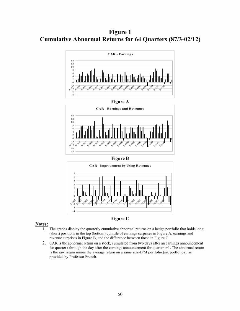
Figure 1 Cumulative Abnormal Returns for 64 Quarters (87/3-02/12)
CAR - Earnings
-8-6-4-202468
101214
3-198
7
3-198
8
3-198
9
3-199
0
3-199
1
3-199
2
3-199
3
3-199
4
3-199
5
3-199
6
3-199
7
3-199
8
3-199
9
3-200
0
3-200
1
3-200
2
Figure A
CAR - Earnings and Revenues
-8-6-4-202468
101214
3-198
7
3-198
8
3-198
9
3-199
0
3-199
1
3-199
2
3-199
3
3-199
4
3-199
5
3-199
6
3-199
7
3-199
8
3-199
9
3-200
0
3-200
1
3-200
2
Figure B
CAR - Improvement by Using Revenues
-4-3-2-10123456
3-198
7
3-198
8
3-198
9
3-199
0
3-199
1
3-199
2
3-199
3
3-199
4
3-199
5
3-199
6
3-199
7
3-199
8
3-199
9
3-200
0
3-200
1
3-200
2
Figure C
Notes: 1. The graphs display the quarterly cumulative abnormal returns on a hedge portfolio that holds long
(short) positions in the top (bottom) quintile of earnings surprises in Figure A, earnings and revenue surprises in Figure B, and the difference between those in Figure C.
2. CAR is the abnormal return on a stock, cumulated from two days after an earnings announcement for quarter t through the day after the earnings announcement for quarter t+1. The abnormal return is the raw return minus the average return on a same size-B/M portfolio (six portfolios), as provided by Professor French.
50