Do Firms Want to Borrow More?

Testing Credit Constraints Using a Directed Lending Program∗

Abhijit V. Banerjee†and Esther Duflo‡

Revised: August 2004

Abstract

We begin the paper by laying out a simple methodology that allows us to determine

whether firms are credit constrained, based on how they react to changes in directed lending

programs. The basic idea is that while both constrained and unconstrained firms may be

willing to absorb all the directed credit that they can get (because it may be cheaper than

other sources of credit), constrained firms will use it to expand production, while uncon-

strained firms will primarily use it as a substitute for other borrowing. We then apply this

methodology to firms in India that became eligible for directed credit as a result of a policy

change in 1998, and lost eligibility as a result of the reversal of this reform in 2000. Using

firms that were already getting this kind of credit before 1998, and retained eligibility in 2000

to control for time trends, we show that there is no evidence that directed credit is being

used as a substitute for other forms of credit. Instead the credit was used to finance more

production—there was significant acceleration in the rate of growth of sales and profits for

these firms. We conclude that many of the firms must have been severely credit constrained.

Keywords: Banking, Credit constraints, India JEL: O16, G2

∗We thank Tata Consulting Services for their help in understanding the Indian banking industry,

Sankarnaranayan for his work collecting the data, Dean Yang and Niki Klonaris for excellent research assistance,

and Robert Barro, Sugato Battacharya, Gary Becker, Shawn Cole, Ehanan Helpman, Sendhil Mullainathan,

Kevin Murphy, Raghuram Rajan and Christopher Udry for very useful comments. We are particularly grateful

to the administration and the employees of the bank we studied for their giving us access to the data we use in

this paper.†Department of Economics, MIT and BREAD.‡Department of Economics, MIT, NBER, CEPR and BREAD.

1

1 Introduction

That there are limits to access to credit is widely accepted today as an important part of an

economist’s description of the world. Credit constraints now figure prominently in economic

analyses of short-term fluctuations and long-term growth.1 Yet one is hard-pressed to find

tight evidence of the existence of credit constraints on firms, especially in a developing country

setting. While there is evidence of credit constraints in rural settings in developing countries,

credit constraints are unlikely to have large productivity impacts unless they also affect firms.

The difficulty of establishing evidence of credit constraints is in some ways what is to be

expected: A firm is credit constrained when it cannot borrow as much as it would like to at the

going market rate, or, in other words, when the marginal product of capital in the firm is greater

than the market interest rate. It is, however, not clear how one should go about estimating the

marginal product of capital. The most obvious approach, which relies on using shocks to the

market supply curve of capital to estimate the demand curve, is only valid under the assumption

that supply is always equal to demand, i.e., if the firm is never credit constrained.

The literature has therefore taken a less direct route: The idea is to study the effects of

access to what are taken to be close substitutes for credit–current cash flow, parental wealth,

community wealth–on investment. If there are no credit constraints, greater access to a substi-

tute for credit would be irrelevant for the investment decision. While this literature has typically

found that these credit substitutes do affect investment,2 suggesting that firms are indeed credit

constrained, the interpretation of this evidence is not uncontroversial. The problem is that ac-

cess to these other resources is likely to be correlated with other characteristics of the firm (such

as productivity) that may influence how much it wants to invest. For example, a shock to cash

flow potentially contains information about the firm’s future performance. Of course, if one has

enough information about the shock, one can isolate shocks that contain no information on the

1See Bernanke and Gertler (1989) and Kiyotaki and Moore (1997) on theories of business cycles based on credit

constraints and Banerjee and Newman (1993) and Galor and Zeira (1993) on theories of growth and development

based on limited credit access.2The literature on the effects of cash-flow on investment is enormous. Fazzari, Hubbard and Petersen (1998)

provide a useful introduction to this literature. The effects of family wealth on investment have also been exten-

sively studied (see Blanchflower and Oswald (1998), for an interesting example). There is also a growing literature

on the effects on community ties on investment (see, for example, Banerjee and Munshi (2004)).

1

prospects of the firm. Lamont’s (1997) use of oil-price shocks to look at non-oil investment of

oil companies is an example of this strategy. However, it is not an accident that the companies

for which Lamont is able to have precise enough information about the nature of shocks tend to

be very large companies and, as emphasized by Lamont and others,3 cash flow shocks can have

very different effects on big, cash-rich firms than on small, cash-poor firms.4

Here we take a different approach to this question. We make use of a policy change that

affected the flow of directed credit to an identifiable subset of firms. Such policy changes are

common in many developing and developed countries–even the U.S. has the Community Rein-

vestment Act, which obliges banks to lend more to specific communities.

The advantage of our approach is that it gives us a specific exogenous shock to the supply of

credit to specific firms (as compared to a shift in the overall supply of credit). Its disadvantage

is that directed credit need not be priced at its true market price, and therefore a shock to the

supply of directed credit might lead to more investment even if a firm is not credit constrained.

In this paper we develop a simple methodology based on ideas from elementary price theory

that allows us to deal with this problem. The methodology is based on two observations: First,

if a firm is not credit constrained, then an increase in the supply of subsidized directed credit

to the firm must lead it to substitute directed credit for credit from the market. Second, while

investment and therefore total production may go up even if the firm is not credit constrained,

it will only go up if the firm has already fully substituted market credit with directed credit.

We test these implications using firm-level data that we collected from a sample of small to

medium size firms in India. We make use of a change in the so-called priority sector regulation,

under which firms smaller than a certain limit are given priority access to bank lending.5 The

first experiment we exploit is a 1998 reform which increased the maximum size below which a

firm is eligible to receive priority sector lending. Our basic empirical strategy is a difference-

3Kaplan and Zingales (2000) make the same point.4The estimation of the effects of credit constraints on farmers is significantly more straightforward since

variations in the weather provide a powerful source of exogeneous short-term variation in cash flow. Rosenzweig

and Wolpin (1993) use this strategy to study the effect of credit constraints on investment in bullocks in rural

India.5Banks are penalized for failing to lend a certain fraction of the portfolio to firms that are classified to be in

the priority sector.

2

in-difference-in-difference approach, That is, we focus on the changes in the rate of change in

various firm outcomes before and after the reform for firms that were included in the priority

sector as a result of the new limit, using the corresponding changes for firms that were already

in the priority sector as a control. We find that bank lending and firm revenues went up for the

newly targeted firms in the year of the reform. We find no evidence that this was accompanied

by substitution of bank credit for borrowing from the market and no evidence that revenue

growth was confined to firms that had fully substituted bank credit for market borrowing. As

already argued, the last two observations are inconsistent with the firms being unconstrained in

their market borrowing. Our second experiment uses the fact that a subset of the firms that were

included in the priority sector in 1998 were excluded again in 2000. We find that bank lending

and firm revenues went down for these firms, both compared to the firms that had always been

part of the priority sector and to firms that were included in 1998, and remained part of the

priority sector in 2000. This second experiment makes it unlikely that the results we obtain are

an artifact of differential trends for large, medium and small firms.

We also use this data to estimate parameters of the production function. We find no clear

evidence of diminishing returns to additional investment, which reinforces the idea that the firms

are not at the point where the marginal product is about to fall below the interest rate. Finally,

we try to estimate the effect of the program-induced additional investment on profits. While

the interpretation of this result relies on some additional assumptions, it suggests a very large

gap between the marginal product and the interest rate paid on the marginal dollar (the point

estimate is that Rs. 1 more in loans increased profits net of interest payment by Rs. 0.73, which

is much too large to be explained as just the effect of receiving a subsidized loan).

The rest of the paper is organized as follows: The next section describes the institutional

environment and our data sources, provides some descriptive evidence and informally argues that

firms may be expected to be credit constrained in this environment. The next section develops

our empirical strategy, starting with the theory and ending with the equations we estimate.

The penultimate section reports the results. We conclude with some admittedly speculative

discussion of what our results imply for credit policy in India.

3

2 Institutions, Data and Some Descriptive Evidence

2.1 The Banking Sector in India

Despite the emergence of a number of dynamic private sector banks and entry by a large number

of foreign banks, the biggest banks in India are all in the public sector, i.e., they are corporatized

banks with the government as the controlling share-holder. The 27 public sector banks collect

over 77% of deposits and comprise over 90% of all branches.

The particular bank we study is a public sector bank. While we are bound by confidentiality

requirements not to reveal the name of the bank, we note it was rated among the top five public

sector banks for several of the past few years by Business Today, a major business magazine.

While banks in India occasionally provide longer-term loans, financing fixed capital is primar-

ily the responsibility of specialized long-term lending institutions such as the Industrial Finance

Corporation of India. Banks typically provide short-term working capital to firms. These loans

are given as a credit line with a pre-specified limit and an interest rate that is set a few per-

centage points above prime. The spread between the interest rate and the prime rate is fixed in

advance based on the firm’s credit rating and other characteristics, but cannot be more than 4%.

Credit lines in India charge interest only on the part that is used and, given that the interest

rate is pre-specified, many borrowers want as large a credit line as they can get.

2.2 Priority Sector Regulation

All banks (public and private) are required to lend at least 40% of their net credit to the “priority

sector”, which includes agriculture, agricultural processing, transport industry, and small scale

industry (SSI). If banks do not satisfy the priority sector target, they are required to lend money

to specific government agencies at very low rates of interest.

In January 1998, there was a change in the definition of the small scale industry sector.

Before this date, only firms with total investment in plant and machinery below Rs. 6.5 million

were included. The reform extended the definition to include firms with investment in plants

and machinery up to Rs. 30 million. In January 2000, the reform was partially undone by a

new change: Firms with investment in plants and machinery between Rs. 10 million and Rs. 30

million were excluded from the priority sector.

4

The priority sector targets seem to be binding for the bank we study (as well as for most

banks): Every year, the bank’s share lent to the priority sector is very close to 40% (it was 42% in

2000-2001). It is plausible that the bank had to go some distance down the client quality ladder

to achieve this target. Moreover, there is the issue of the physical cost of lending. Banerjee and

Duflo (2000) calculated that, for four Indian public banks, the labor and administrative costs

associated with lending to the SSI sector were 22 Paisa per Rupee lent, or about 1.5 Paisa higher

than that of lending in the unreserved sector. This is consistent with the common view that

lending to smaller clients is more costly.

Two things changed when the priority sector limit was raised: First, the bank could draw

from a larger pool and therefore could be more exacting in its standards for clients. Second, it

could save on the cost of lending by focusing on slightly larger clients. For both these reasons

the bank would like to switch its lending towards the newly inducted members of the priority

sector. If these firms were constrained in their demand for credit before the policy change, one

would expect to see an expansion of lending to these firms relative to firms that were already in

the priority sector.6 When firms with investment in plant and machinery above 10 million Rs.

were excluded again from the priority sector, loans to these firms no longer counted towards the

priority sector target. The bank had to go back to the smaller clients to fulfill its priority sector

obligation. One therefore expects that loans to those firms declined relative to the smaller firms.

2.3 Data Collection

The data for this study were obtained from one of the better-performing Indian public sector

banks. This bank, like other public sector banks, routinely collects balance sheet and profit

and loss account data from all firms that borrow from it and compiles the data in the firm’s

loan folder. Every year the firm also must apply for renewal/extension of its credit line, and

the paperwork for this is also stored in the folder, along with the firm’s initial application, even

when there is no formal review of the file. The folder is typically stored in the branch until it is

6The increase in lending to larger firms may come entirely at the expense of smaller firms (without affecting

total lending to the priority sector), or the reform could cause an increase in the amount lent to the priority

sector. We will focus on the comparison between firms that were newly labelled as priority sector and smaller

firms.

5

physically impossible to put more documents in it.

With the help of employees from this bank, as well as a former bank officer, we first extracted

data from the loan folders in the spring of 2000. We collected general information about the

client (product description, investment in plant and machinery, date of incorporation of units,

length or the relationship with the bank, current limits for term loans, working capital, and letter

of credit). We also recorded a summary of the balance sheet and profit and loss information

collected by the bank, as well as information about the bank’s decision regarding the amount of

credit to extend to the firm and the interest rate charged.

As we discuss in more detail below, part of our empirical strategy called for a comparison

between accounts that have always been a part of the priority sector and accounts that became

part of the priority sector in 1998. We first selected all the branches that handle business

accounts in the six major regions of the bank’s operation (including New Delhi and Mumbai).

In each of these branches, we collected information on all the accounts that were included in

the priority sector after January 1998 (these are the accounts for which the investment in plant

and machinery is between 6.5 and 30 million Rupees). We collected data on a total of 249 firms,

including 93 firms with investment in plants and machinery between 6.5 and 30 million Rupees.

We aimed to collect data for the years 1996-1999, but when a folder is full, older information

is not always kept in the branch. Every year, there are a few firms from which the data was

not collected. We have 1996 data on lending for 120 accounts (of the 166 firms that had started

their relationship with the bank by 1996), 1997 data for 175 accounts (of 191 possible accounts),

1998 data for 217 accounts (of 238), and 1999 data for 213 accounts. In the winter 2002-2003,

we collected a new wave of data on the same firms in order to study the impact of the priority

sector contraction on loans, sales and profits. We have 2000 data for 175 accounts, 2001 data

for 163 accounts, and 2002 data for 124 accounts.7

Table 1 presents the summary statistics for all data used in the analysis of credit constraint

7The reason why we have less data in 2000, 2001 and 2002 than in 1999 is that some firms had not had their

2002 review when we re-surveyed them late 2002, and 43 accounts were closed between 2000 and 2002. The

proportion of accounts closed is balanced: It is 15% among firms with investment in plant and machinery above

10 million, 20% among firms with investment in plant and machinery between 6.5 and 10 million, and 20% among

firms with investment in plant and machinery below 6.5 million. Thus, it does not appear that sample selection

bias would emerge from the closing of those accounts.

6

and credit rationing (in the full sample, and in the sample for which we have information on the

change in lending between the previous period and that period, which is the sample of interest

for the analysis).

2.4 Descriptive Evidence on Lending Decisions

In this subsection, we provide some description of lending decisions in the banking sector. We use

this evidence to argue that this is an environment where credit constraints arise quite naturally.

Tables 2 and 3 show descriptive statistics regarding the loans in the sample. The first row

of table 2 shows that, in a majority of cases, the loan limit does not change from year to year:

In 1999, the limit was not updated even in nominal terms for 65% of the loans. This is not

because the limit is set so high that it is essentially non-binding: row 2 shows that in the six

years in the sample, 63% to 80% of the accounts reached or exceeded the credit limit at least

once in the year.

This lack of growth in the credit limit granted by the bank is particularly striking given that

the Indian economy registered nominal growth rates of over 12% per year. This would suggest

that the demand for bank credit should have increased from year to year over the period, unless

the firms have increasing access to another source of finance. There is no evidence that they

were using any other formal source of credit. On average, 98% of the working capital loans

provided to firms in our sample come from this one bank, and, in any case, the same kind of

inertia shows up in the data on total bank loans to the firm.

That the demand for formal sector credit increased from year to year is suggested by rows 3

to 5 in table 2. The bank’s official guidelines for lending explicitly state that the bank should try

to meet the legitimate needs of the borrower. For this reason, the maximum lending limits that

can be authorized by the bank for working capital loans are explicitly linked to the projected

sales of the borrower—the maximum limit is supposed to be one-fifth of the predicted sales for

the year. Every year, a bank officer must approve a sales projection for the firm and calculate

a maximum lending limit on the basis of the turnover.8 Projected sales therefore provide a

measure of the credit needs of the firm. Row 3 shows that actual sales have increased from8The exact rule is that the limit on turnover basis should be the minimum of 20% of the projected sales and

25% of the projected sales minus the finances available to the firm from other sources.

7

year to year for most firms. Rows 4 and 5 show that both projected sales and the maximum

authorized lending also increased from year to year in a large majority of cases. Yet there was

no corresponding change in lending from the bank. The change in the credit limit that was

actually sanctioned systematically fell short of what the bank determined to be the firm’s needs

as determined by the bank. In 1999, 80% of the actual limits granted were below 20% of the

predicted sales, and 60% were below the maximum limit calculated by the bank. On average,

the granted limit was 89% of the recommended limit, and 67% of what following the rule based

on 20% of predicted sales would give. It is possible that some of the shortfall was covered by

informal credit, including trade credit: According to the balance sheet, total current liabilities

excluding bank credit increased by 3.8% every year on average. However, some expenses (such

as wages) are typically not covered by trade credit and, moreover, trade credit could be rationed

as well. The question that is at the heart of this paper is whether such substitution operates to

the point where a firm is not credit constrained.

In table 3, we examine in more detail whether this tendency could be explained by other

factors that might have affected a firm’s need for credit. Column (3) shows that no variable we

observe seems to explain why a firm’s credit limit was changed: Firms are not more likely to get

an increase in limit if they reached the maximum limit in the previous year, if their projected

sales (according to the bank itself ) have increased, if their current sales have increased, if the

ratio of profits to sales has increased, or if the current ratio (the ratio of current assets to current

liabilities, a traditional indicator of how secure a working capital loan is, in India as well as in

the U.S.) has increased. Turning to the direction or the magnitude of changes, only an increase

in projected sales or current sales predicts an increase in granted limit, and only an increase in

projected sales predict the level of increase. This could well be due to reverse causality, however:

The bank officer could be more likely to predict an increase in sales when he is willing to give a

larger credit extension to the firm.

One reason the granted limit may not change is that the previous year’s limit already incor-

porated all information relevant to the lending decision: The limit is not responsive to what is

currently going on in the firm, because these are just short-run fluctuations which tell us little

about the future of the firm. If this were the case, we should observe that granted limits are

much more responsive to these factors for young firms than for old firms. Columns 5 and 6

8

in table 3 repeat the analysis, breaking the sample into recent and older clients. Changes in

limits are more frequent for younger clients, but they do not seem to be more sensitive to past

utilization, increases in projected sales, or profits.

The fact that the probability of a limit’s change is uncorrelated with observable firm char-

acteristics is striking. One plausible theory relates this to the fact, noted above, that changes in

the limit are surprisingly rare. If bank officials are reluctant to change the limit, a large fraction

of the observed changes may reflect effective lobbying or something purely procedural (“it has

been five years since the limit was raised”) rather than economic rationality.

What explains the reluctance of loan officers to do what is, palpably, their job? A recent

report on banking policies commissioned by the Reserve Bank of India suggests one potential

explanation: “The [working group] observed that it has received representations from the man-

agement and the unions of the bank complaining about the diffidence in taking credit decisions

with which the banks are beset at present. This is due to investigations by outside agencies

on the accountability of staff in respect to Non-Performing Assets.” (Tannan (2001)). In other

words, the problem is that changing the limit (in either direction) involves sticking one’s neck

out—if one cuts the limit the firm may complain, and if one raises it, there is a possibility one

would be held responsible if the loan goes bad: The Central Vigilance Commission (a govern-

ment body entrusted with monitoring the probity of public officials) is formally notified of every

instance of a bad loan in a public sector bank, and investigates a fraction of them.9 Consistent

with this “fear of lending” explanation, Banerjee, Cole and Duflo (2004) show that lending slows

down whenever there is an investigation against an credit officer in a given bank.

Simply renewing a loan without changing the amount is one easy way to avoid such re-

sponsibility, especially if the original decision was someone else’s (loan officers are frequently

transferred). The problem is likely exacerbated by the fact that the link between the prof-

itability of the bank and the career prospects of an individual loan officer, is, at best, rather

weak.

It should be emphasized, however, that while the fact that our bank is in the Indian public

sector may have exacerbated the problem, the core tension here is quite universal. All banks of

9There were 1,380 investigations of bank officers in 2000 for credit related frauds, 55% of which resulted in

major sanctions.

9

any size deal with the problem that the officer who decides whether or not make a loan does

not have very much to lose if the loan goes bad, while the bank could stand to lose a lot. They

deal with it by limiting the discretion that the officer has (by requiring that he use a scoring

model, for example) and by penalizing officers whose loans go bad, who in turn respond by not

taking any more chances than they have to. For both these reasons, certain firms will not be

able to get the credit that they want from the bank (see Stein (2002) for a model that makes

this point).

The fact that the bank in our data does not seem to be responding to changes in firms’ credit

needs, suggests that some firms would have an unmet demand for credit from this particular bank.

It does not prove that the firm will be credit constrained: After all, there are other banks, and

other sources of credit (such as trade credit). Nevertheless, it does make it more plausible.

3 Establishing Credit Constraints

3.1 Theory

Consider a firm with the following fairly standard production technology: The firm must pay

a fixed cost C before starting production (say the cost of setting up a factory and installing

machinery). The firm then invests in labor and other variable inputs. k rupees of working

capital invested in variable inputs yield R = F (k) rupees of revenue after a suitable period.

F (k) has the usual shape–it is increasing and concave.

As mentioned above, we need to consider the case where the firms have multiple sources of

credit. We will say that a firm is credit rationed with respect to a particular lender if there is no

interest rate r such that the amount the firm wants to borrow at that rate is strictly positive and

equal to an amount that the lender is willing to lend at that rate.10 Essentially this says that

the supply curve of loans from that lender to the firm is not horizontal at some fixed interest

rate.

We will say the firm is credit constrained if there is no interest rate r such that the amount

that the firm wants to borrow at that rate is equal to an amount that all the lenders taken

10The amount the firm wants to borrow at a given rate is assumed to be an amount that would maximize the

firm’s profit if it could borrow as much (or as little) as it wants at that rate.

10

together are willing to lend at that rate. This says that the aggregate supply curve of capital to

the firm is not horizontal at some fixed interest rate.

Note that a firm could be credit rationed with respect to every lender without being credit

constrained in our sense. This can be the case, for example, when there is an infinite supply of

lenders, each willing to lend to no more than $10 at an interest rate of 10%.

It is convenient to begin with the simple case where there are only two lenders, which we

will call the “market" and the bank. Denote the market rate of interest by rm and the interest

rate that the bank charges by rb. Given that the bank is statutorily required to lend a certain

amount to the priority sector, there is reason to believe that the bank lending rate is below the

market rate: rb ≤ rm.

The policy change we analyze involves the firms in question being offered additional bank

credit. We will show in the next section that there was no corresponding change in the interest

rate. To the extent that firms accepted the additional credit being offered to them, this is direct

evidence of credit rationing with respect to the bank. However this in itself does not imply that

they would have borrowed more at the market interest rate. A possible scenario is depicted in

figure 1. The horizontal axis in the figure measures k while the vertical axis represents output.

The downward sloping curve in the figure represents the marginal product of capital, F 0(k). The

step function represents the supply of capital. In the case represented in the figure, we assume

that the firm has access to kb0 units of capital at the bank rate rb but was free to borrow as

much as it wanted at the higher market rate rm. As a result, it borrowed additional resources

at the market rate until the point where the marginal product of capital is equal to rm. Its

total outlay in this equilibrium is k0. Now consider what happens if the firm is now allowed to

borrow a greater amount, kb1, at the bank rate. Since at kb1 the marginal product of capital is

higher than rb, the firm will borrow the entire additional amount offered to it. Moreover, it will

continue to borrow at the market interest rate, though the amount is now reduced. The total

outlay, however, is unchanged at k0. This will remain the case as long as kb1 < k0: The effect of

the policy will be to substitute market borrowing with bank loans. The firms profits will go up

because of the additional subsidies, but its total outlay and output will remain unchanged.

The expansion of bank credit will have output effects in this setting if kb1 > k0. In this case,

the firm will stop borrowing from the market and the marginal cost of credit it faces will be

11

rb. It will borrow as much it can get from the bank but no more than kb2, the point where the

marginal product of capital is equal to rb. We summarize these arguments in:

Result 1: If the firm is not credit constrained (i.e., it can borrow as much as it wants at

the market rate), but is rationed for bank loans, an expansion of the availability of bank credit

should always lead to a fall in its borrowing from the market as long as rb < rm. Profits will

also go up as long as market borrowing falls. However, the firm’s total outlay and output will

go up only if the priority sector credit fully substitutes for its market borrowing. If rb = rm, the

expansion of the availability of bank credit will have no effect on outlay, output or profits.

We contrast this with the scenario in figure 2, where the assumption is that the firm is

rationed in both markets and is therefore credit constrained. In the initial situation, the firm

borrows the maximum possible amount from the banks (kb0) and supplements it with borrowing

the maximum possible amount from the market, for a total investment of k0. Available credit

from the bank then goes up to kb1. This has no effect on market borrowing (since the total

outlay is still less than what the firm would like at the rate rm), and therefore total outlay

expands to k1. There is a corresponding expansion of output and profits.11

Result 2: If the firm is credit constrained, an expansion of the availability of bank credit

will lead to an increase in its total outlay, output and profits, without any change in market

borrowing.

We have assumed a particularly simple form of the credit constraint. However, both results

hold if instead of the strict rationing we have assumed here the firms face an upward supply

curve for bank credit. The result also holds if there are more than two lenders, as long we

interpret it to be telling us what happens to the more expensive sources of credit when the

supply of cheap credit is expanded.

The fact that the supply curve of market credit is drawn as a horizontal in figure 2 is

also not important–what is important is that the supply curve of market credit in this figure

eventually becomes vertical. More generally, the key distinction between figure 1 and figure 2

is that in figure 1, the supply curve of market credit is always horizontal (which is why the

firm is unconstrained), while in figure 2 the supply curve slopes up (which is why the firm is

11Of course, if kp1 were so large that F 0(kp1) < rm, then there would be substitution of market borrowing in

this case as well.

12

constrained).

The results also go through if the market supply curve of credit is itself a function of bank

credit (for example because bank credit serves as collateral for market credit). In this case, there

might be an increase in market borrowing as the result of the reform but this should be counted

as a part of the effect of the reform.

One case (pointed out by a referee of a previous version of this paper) where these results

fail is when the firm can borrow as much as it wants from the market but not as little as it

wants (because it wants to keep an ongoing credit relationship with this source). If the minimum

market borrowing constraint takes the form of a minimum share of total borrowing that has to

be from the market and this constraint binds, a firm will respond to the availability of extra

bank credit by also borrowing more from the market, in order to maintain the required minimum

share of market borrowing. In this case, our result 1 will fail. However, as long as there are some

firms that are not at this constraint, there will be some substitution of bank credit for market

credit. Therefore the direct test of substitution, proposed below, would apply even in this case,

as long as the minimum market borrowing constraint does not bind for all the firms.

3.2 Empirical Strategy: Reduced Form Estimates

The empirical work follows directly from the previous subsection and seeks to establish the

facts that will allow us to determine whether firms are credit rationed and to distinguish credit

rationing from credit constraint.

Our empirical strategy takes advantage of the extension of the priority sector definition in

1998 and its subsequent contraction in 2000. As we described above, the reform extended the

definition of the priority sector to firms with investment in plants and machinery between Rs.

6.5 and 30 million. In 2000, firms with investment in plant and machinery above 10 million

were excluded from the priority sector. As we noted, since the priority sector target (40% of the

lending portfolio) was binding for our bank before and after this reform, there is good reason to

believe that the reform reduced the shadow cost of lending for the bigger firms newly included in

the priority sector and thus resulted in an increase in their credit. Conversely, the 2000 reform

increased the shadow cost of lending for firms with investment in plant and machinery between

10 and 30 million and should have resulted in a decrease in credit to these firms. The reform did

13

not seem to have large effects on the composition of clients of the banks: In the sample, 25% of

the small firms and 28% of the big firms have entered their relationship with the bank in 1998

or 1999. This suggests that the bank was no more likely to take on big firms after the reform

and that our results will not be affected by sample selection.

Since the granted limit as well as all the outcomes we will consider, are very strongly auto-

correlated, we focus on the proportional change in this limit, i.e., log(limit granted in year t)−

log(limit granted in year t-1).12 Table 4 shows the average change in the credit limit faced by

the firm in the three periods of interest (loans granted before the change in January 1998,

between January 1998 and January 2000, after January 2000) separately for the largest firms

(investment in plant and machinery above Rs. 10 million), the medium-sized firms (investment

in plant and machinery between Rs. 6.5 and Rs. 10 million), and the smaller firms (investment

in plant and machinery below Rs. 6.5 million).

For limits granted in 1997 the average increase in the limit was 7% larger for the small firms

than for medium firms, and 2% larger than for the biggest firms. For limits granted in 1998 and

1999, it was 2% larger for medium firms, and 7% larger for the biggest firms. In fact, the size

of the average increase in the limit grew for medium and large firms and shrunk for the small

ones. After 2000, limit increases were smaller for all firms, but the biggest declined happened

for the larger firms, whose enhancement declined from an average of 14% in 1998 and 1999 to

0% in 2000.

Panel B in table 4 shows that the average increase in the limit was not due to an increase

in the probability that the working capital limit was changed: Big firms were no more likely to

experience a change in 1998 or 1999 than in 1997. This may appear surprising, but it is entirely

consistent with the previous evidence showing that it is not possible to explain why certain firms

experienced a change in their credit limit. It is plausible that bureaucratic inertia was at work

here as well. While loan officers needed to respond to pressure from the bank to expand lending

to the newly eligible big firms, they seem to have preferred giving larger increases to those which

would have received an increase in any case (for one reason or another), rather than increasing

the number of firms whose limits are increased.12Since the source of variation in this paper is closely related to the size of the firm, we express all the variables

in log to avoid spurious scale effects.

14

In Panel C, we show the average increase in limit, conditional on the limit changing. The

average percentage enhancement was larger for the small firms than the medium and large firms

in 1997, smaller for the small firms than for the large firms in 1998 and 1999 (and about the

same for the medium firms), and larger after 2000. The average enhancement conditional on a

change in limit declined dramatically for the largest firm after 2000 (it went from an average of

0.44 to an average of slightly less than 0).

Our strategy will be to use these two changes in policy as a source of shock to the availability

of bank credit to the medium and larger firms, using firms outside this category to control for

possible trends. The first step, however, is to formally establish that there was indeed such a

shock. To do this we first use the data from 1997 to 2000 an estimate and equation of the form:13

log kbit − log kbit−1 = α1kbBIGi + β1kbPOST + γ1kbBIGi ∗ POSTt + 1kbit, (1)

where we adopt the following convention for the notation: kbit is a measure of bank credit to

firm i in year t (and therefore granted, i.e., decided upon, some time during the year t − 114),

BIG is a dummy indicating whether the firm has investment in plant and machinery between

Rs. 6.5 million and Rs. 30 million, and POST is a dummy equal to one in the years 1999 and

2000 (The reform was passed in 1998. It therefore affected the credit decisions for the revision

conducted during the years 1998 and 1999, affecting the credit available in 1999 and 2000). We

focus on working capital loans from this bank.15 We estimate this equation in the entire sample

and in the sample of accounts for which there was no revision in the amount of the loan. We

expect a positive γ1b.

To study the impact of the contraction of the priority sector on bank loans, we use the

1999-2002 data and estimate the following equation:

log kbit − log kbit−1 = α2kbBIG2i + β2kbPOST2 + γ2kbBIG2i ∗ POST2t + 2kbit, (2)

where BIG2 is a dummy indicating whether the firm has investment in plant and machinery

13All the standard errors are clustered at the sector level.14Seventy percent of the credit reviews happen during the last six months of the year, including 15% in December

alone.15Using total working capital loans from the banking sector instead leads to almost identical results.

15

between Rs. 10 millions and Rs. 30 millions, and POST2 is a dummy equal to one in the years

2001 and 2002.16

Finally, we pool the data and estimate the equation:

log kbit − log kbit−1 = α3kbBIG2i + α4kbMEDi + β3kbPOST + β4kbPOST2 +

γ3kbBIG2i ∗ POSTt + γ4kbMEDi ∗ POSTt +

γ5kbBIG2i ∗ POST2t + γ6kbMEDi ∗ POST2t + 3kbit, (3)

whereMED is a dummy indicating that the firm’s investment in plant and machinery is between

Rs. 6.5 million and Rs. 10 million.

As pointed out in the previous subsection, the impact of the shock on the firm depends

crucially on whether the firm was credit constrained, credit rationed or entirely unconstrained.

In order to distinguish between these cases we need to look at a number of other credit variables

for the firm. We therefore run a number of other regressions that exactly parallel equations (1)

to (3). First, we use the sample 1997-2000 to estimate:

yit − yit−1 = α1yBIGi + β1yPOSTt + γ1yBIGi ∗ POSTt + 1yit, (4)

where yit is an outcome variable (such as credit, sales, or cost) for firm i in year t. Second, we

estimate:

log yit − log yit−1 = α2yBIG2i + β2yPOST2 + γ2yBIG2i ∗ POST2t + 2yit, (5)

in the sample 1999-2002 , and finally we estimate:

log yit − log yit−1 = α3yBIG2i + α4yMEDi + β3yPOST + β4yPOST2 +

γ3yBIG2i ∗ POSTt + γ4yMEDi ∗ POSTt +

+γ5yBIG2i ∗ POST2t + γ6yMEDi ∗ POST2t + 3yit (6)

16Once again, we adopt the convention that we look at credit available in year t, and therefore granted in year

t−1. The reform was passed in 2000 and therefore affected credit decisions taken during the year 2000 and credit

available in the year 2001.

16

in the pooled sample.

Below, we describe the variables we use and their justification.

• Credit rationing

Our Result 1 above suggests that to establish credit rationing we need two pieces of evidence

in addition to the evidence on the expansion of bank loans.

First, since the working capital loans take the form of a line of credit (and firms are charged

only for what they use), we need to examine what happened to the rate at which firms draw

upon their granted limit. We thus use as our measure of credit utilization the logarithm of the

ratio of total borrowing under the line of credit divided by the limit.

Second, this would not be evidence of credit rationing if the interest rate charged on this

loan decreased at the same time. Priority sector loans are not supposed to have lower interest

rates (the interest rate charged on a loan is the prime lending rate plus a premium depending

on the credit rating of the firm—without regard for its status), so there is no prima facie reason

the rate should fall. However, we directly check whether there is evidence of this using three

specifications: Using yit = rbit in equation (4) and (5), for rbit equal to the interest rate in

logarithm and in level, and replacing yit − yit−1 in equation (4) and (5) by a dummy indicating

whether the interest rate fell.

• Credit constraints

Credit rationing does not necessarily imply credit constraint. To establish that the firms

were indeed credit constrained, we look at a number of other pieces of evidence.

First, if a firm were credit constrained, our theory tells us that sales revenue would definitely

go up, while if it were not, sales should only go up for firms that have already fully substituted

bank credit for their market borrowing. To look at the effect of credit expansion on sales, we

posit a simple parametric relation between credit and sales revenue: Rit = Aitkθit. Note that this

is a specific parametrization of the production function introduced in the previous sub-section:17

logRit = logAit + θ log kit. (7)

17This is best thought of as a reduced form, derived from a more primitive technology which makes output a

Cobb-Douglas function of the amount of n inputs x1, x2...xn. As long as the inputs have to purchased using the

working capital, and all inputs are purchased in competitive markets, it can be shown that the resulting indirect

production function has the form given above.

17

Differencing this equation gives:

logRit − logRit−1 = logAit − logAit−1 + θ[log kit − log kit−1]. (8)

Focusing on the first experiment (credit expansion), we have already posited that the growth

of bank credit between 1997 and 1999 is given by:18

log kbit − log kbit−1 = α1kbBIGi + β1kbPOSTt + γ1kbBIGi ∗ POSTt + 1kbit. (9)

In the absence of complete substitution between bank credit and market credit, this implies

a relationship of the same shape for capital stock:

log kit − log kit−1 = α1kBIGi + β1kPOSTt + γ1kBIGi ∗ POSTt + 1kit, (10)

which when substituted in equation (8) yields

logRit−logRit−1 = logAit−logAit−1+θ[α1kBIGi+β1kPOSTt+γ1kBIGi∗POSTt+ 1kit]. (11)

Since we do not observe logAit − logAit−1 directly, we end up estimating an equation that

exactly mimics equation 4 above:

logRit − logRit−1 = α1RBIGi + β1RPOSTt + γ1RBIGi ∗ POSTt + 1kit. (12)

Our identification hypothesis is that:

logAit − logAit−1 = α1ABIGi + β1APOSTt. (13)

This amounts to assuming that the rate of change of A (which is a shift parameter in the

production function) did not change differentially for big and small firms in the year of the

priority sector expansion. Under this assumption, γR gives the reduced form effect of the

expansion of the priority sector on sales revenue.

Similar calculations lead to an equation of the same form, similar to equation (6) for the

priority sector contraction (1998-2002):

logRit − logRit−1 = α2RBIG2i + β2RPOST2t + γ2RBIG2i ∗ POST2t + 2kit, (14)

18As before, POST is a dummy equal to 1 for the year 1999 and 2000 and BIG is a dummy equal to 1 if the

firm has investment in plant and machinery larger than Rs. 6.5 million.

18

where the identification hypothesis is that

logAit − logAit−1 = α2ABIG2i + β2APOST2t. (15)

If firms are credit constrained, γ1R should be positive and γ2R should be negative, while if no

firms are credit constrained γ1R will only be positive for those firms that have fully substituted

market credit, and γ2R will be negative only for those firms that had no market credit initially.

We therefore also estimate a version of equation (12) in the sample of firms whose total current

liabilities exceed their bank credit. If the firms were not credit constrained, the value of γR and

γ2R in this sample should be zero.

A second strategy is to look at substitution directly. Unfortunately we do not have reliable

data on market borrowing. We therefore adopt the following strategy: Equation (8) above can

be rewritten in the form:

logRit/kbit − logRit−1/kbit−1 = logAit − logAit−1

+θ[log kit − log kit−1]− [log kbit − log kbit−1]. (16)

Differencing one more time gives us:

[logRit/kbit − logRit−1/kbit−1]− [logRit−1/kbit−1 − logRit−2/kbit−2]

= [logAit − logAit−1]− [logAit−1 − logAit−2]

+θ([log kit/kbit − log kit−1/kbit−1]− [log kit−1/kbit−1 − log kit−2/kbit−2])

−(1− θ)([log kbit − log kbit−1]− [log kbit−1 − log kbit−2]). (17)

We now take the difference of this expression between big firms and small firms.19 Denoting

by the operator ∆ the operation of difference across firm categories and using (13) we get:

∆{[logRt/kbt − logRt−1/kbt−1]− [logRt−1/kbt−1 − logRt−2/kbt−2]}

= θ∆{([log kt/kbt − log kt−1/kbt−1]− [log kt−1/kbt−1 − log kt−2/kbt−2])}

−(1− θ)∆{[log kbt − log kbt−1]− [log kbt−1 − log kbt−2]}. (18)

19The categories are different for the expansion and for the contraction.

19

We have seen that ∆{[log kbt− log kbt−1]− [log kbt−1− log kbt−2]} is positive when we compare

the year 1998-1999 to the year 1997 and negative when we compare the years 2000-2002 to the

years 1998-1999. If a firm is not credit constrained, it should substitute bank loans for market

loans, which implies that bank capital should grow faster than total capital stock for the big

firms after the expansion, relative to the small firms. Conversely, it should grow less fast for the

biggest firms during the contraction, relative to medium and small firms. During the priority

sector expansion, ∆{([log kt/kbt−log kt−1/kbt−1]−[log kt−1/kbt−1−log kt−2/kbt−2])} is, therefore,

negative. As long as θ ≤ 1, these two observations together imply that the expression on the

right should be negative for firms that are not credit constrained. If θ > 1, this need not

necessarily be case, but with increasing return to scale (which is what θ > 1 gives us) there

cannot be an equilibrium in which the firms are not credit constrained. Conversely, during the

contraction, the expression on the right should be positive for firms that are credit constrained,

if θ ≤ 1.

We implement this by estimating equations (4) to (6) with yit = Ritkbt. If the firm is not credit

constrained, γR/kb should be negative, and γ2R/kb should be positive. If not, we presume that

there is no substitution, implying that the firm is credit constrained.

The impact on sales does not directly inform us on the marginal benefit of the extra invest-

ment.20 A final piece of evidence comes from looking at profits. Denoting kmit as the market

credit of firm i at time t and assuming that the firm buys all its inputs using its working capital,

we can write:

Πit = Ait(kbit + kmit)θ − (1 + rbit)kbit − (1 + rmit(kmit))kmit − C.

We write the supply curve of market credit as rmit(kmit) to recognize the fact that the firm may

be constrained in its access to market credit. It follows that:

d logΠitdt

=Ait(kbit + kmit)

θ

Π

d logAit

dt+

θAit(kbit + kmit)θ−1kbit − (1 + rbit)kbitΠ

d log kbitdt

+θAit(kbit + kmit)

θ−1kmit − (1 + rmit (kmit)) kmit − r0mit(kmit)kmit

Π

d log kmit

dt

−rmitkmit

Π

d log rmit

dt,

ignoring the effect of changes in the bank interest rate, which, given evidence to be shown later,20A “mechanical” manager could simply invest whatever money becomes available to him, for example.

20

does not seem to be much of an issue. Since kmit is optimally chosen, we can drop the third

term in this expression.21 Taking time derivatives again we get:

d2 logΠitdt2

=Ait(kbit + kmit)

θ

Π

d2 logAit

dt2

+θAit(kbit + kmit)

θ−1kbit − (1 + rbit)kbitΠ

d2 log kbitdt2

−rmitkmit

Π

d2 log rmit

dt2.

To get to this expression we dropped all terms which were a product of two rates of change on

the assumption that they are each small and therefore their product will be negligible: d log kbitdt ,

for example, is of the order of 0.1. We do keep the the second derivative terms, because in the

years when there was change in policy d2 log kbitdt2 was of the same order of magnitude as d log kbit

dt .

Comparing big and small firms and invoking the ∆ operator again, we have:

∆{d2 logΠtdt2

} = ∆{At(kbt + kmt)θ

Π}d

2 logAt

dt2+

At(kbt + kmt)θ

Π∆{d

2 logAt

dt2}

−∆{rmtkmt

Π}d

2 log rmt

dt2− rmtkmt

Π∆{d

2 log rmt

dt2}

+∆{θAt(kbt + kmt)θ−1kbt − (1 + rbt)kbtΠ

d2 log kbtdt2

}.

Now d2 log rmt

dt2should be the same for both large and small firms, since it is the market interest

rate.22 Therefore ∆{d2 log rmt

dt2} = 0. During the expansion (1997-1999), by equation 13 above,

∆{d2 logAt

dt2 } = 0. This leaves us with:

∆{d2 logΠtdt2

} = ∆{At(kbt + kmt)θ

Π}d

2 logAt

dt2(19)

−∆{rmtkmt

Π}d

2 log rmt

dt2+∆{θAt(kbt + kmt)

θ−1kbt − (1 + rbt)kbtΠ

d2 log kbtdt2

}.

The last term here is the direct effect of the expansion. Of the other terms, the second term,

∆{ rmtkmtΠ }d2 log rmt

dt2can safely be assumed to be small. It has been shown that, in India, the

21This would not have been possible if we had allowed the supply of market credit to depend on the supply of

bank credit. In that case, there would be an additional term reflecting the effect of bank credit on the supply of

market credit; it would, however, be appropriate to count this term as a part of the impact of the policy change.22Even if the level of market interest rate varies according to firm size, there is no reason for the rate of growth

to vary systematically.

21

average market interest rate is linked to the bank rate. d2 log rmt

dt2is thus closely linked to d2 log rbt

dt2,

which, in the 1997-1999 sample, is given by the POST dummy when we estimate equation (4)

with log(rbt) as the dependent variable. We estimate this coefficient to be -0.010 percentage

point (the average interest rate is 14%).

One scenario where the first term, ∆{At(kbt+kmt)θ

Π }d2 logAt

dt2is small is if d2 logAt

dt2is small. We

can look at this directly because, as shown above, the coefficient on the POST dummy in the

sales equation is a linear combination of d2 logAt

dt2and the coefficient on the POST dummy in the

credit equation. We will show that the POST coefficients in both the credit equation and the

sales equation are essentially zero.23 Together, they suggest that d2 logAt

dt2must be close to zero.

Finally, observe that the last term, ∆{θAt(kbt+kmt)θ−1kbt−(1+rbt)kbtΠ

d2 log kbtdt2 }, may be positive

even if the firm is not credit constrained. This is because rbt ≤ rmt, which allows for the

possibility that θAt(kbt+kmt)θ−1− (1+rbt) > 0 even though At(kbt+kmt)

θ−1kbt− (1+rmt) = 0.

This reflects the fact that profits will go up when the firm has access to more subsidized credit,

even if it is not credit constrained. If the firm is credit constrained, the impact on profits is

greater, because in addition to the subsidy effect there is now a wedge between the market rate

and the marginal product of capital.

It is clear from this discussion that the evidence on profits is unlikely to be definitive. How-

ever, we still estimate equations (4) to (6) with yit = Π ; we expect the coefficient onBIG∗POST

to be strongly positive.

3.3 Empirical Strategy: Testing the Identification assumptions

The interpretation of the central result on sales growth crucially depends on the assumptions

made in equations (13) and (15). Likewise, the interpretation of the other results depend on

the assumption that the error term is not correlated with the regressors, most importantly

BIG ∗ POST in equation (4) and BIG2 ∗ POST2 in equation (5). However, there are many

reasons why this assumption may not hold. For example, big and small firms may be differently

affected by other measures of economic policy (they could belong to different sectors, and these

sectors may be affected by different policies during this period).

The fact that we have two experiments affecting different sets of firms helps in distinguishing

23This is not quite exact, since we do not estimate a total credit equation but only a bank credit equation.

22

the effect of the priority sector regulation from trends affecting different groups of firms differ-

entially. The two reforms went in different directions and did not affect all the firms identically.

Credit constraints would predict γ1y in equation (4) to be positive, γ2y in equation (5) to be

negative, γ3y and γ4y in equation (6) to both be positive, and γ5y and γ6y in the same equation

to be respectively negative and zero.

Equation (11) suggests a straightforward test: The ratiosγ3yγ3kb

,γ4yγ4kb

,γ5yγ5kb

,γ1yγ1kb

andγ2yγ2kb

should all be equal. If all these equalities are satisfied, it would be extremely implausible that

the observed patterns come from the fact that the time trends are different for small and large

firms.

It is still possible that, being labelled as a priority sector firm may affect the sales and

profitability of a firm over and above its effects on credit access. First, SSI firms are exempt

from some types of excise taxation. Second, the right to manufacture certain products is reserved

for the SSI sector. We will address the first concern by using profit before tax in all specifications.

The second concern could be a problem: Among the small firms, 44% manufacture a product

that is reserved for SSI. Among the big firms, 24% do. One control strategy would be to leave out

all firms that manufacture products that are reserved for SSI. Unfortunately, we only know what

products the firms manufactured in 1998. We will show that excluding firms which manufacture

SSI reserved products in 1998 does not change the results. It remains possible that some of the

big firms moved into reserved products after 1998, and this increased their sales and profits.

A more direct way to test our identification assumption (and to improve the precision of the

estimates), is to estimate equations (4) to (6) for the different outcome variables in two sub-

samples: One sub-sample made of the firm-year observations where there was no change in the

granted limit from the previous year to the current year, and one sub-sample made of firms where

there was a change (either an increase or decrease). In doing so, we make use of the fact that the

probability of a change in the limit appears to be unaffected by the policy changes (the variables

BIG ∗ POST and BIG2 ∗ POST2). Given this fact and a simple monotonicity assumption,

estimating an equation of the form of equation (4) separately in the sample where there was a

change in limit and in the sample where there was no change in limit will generate consistent

estimates of the parameter of interest γ in both sub-samples (Heckman (1979); Heckman and

Robb (1986); and Angrist (1995)).

23

The monotonicity assumption restricts the relationship between the instrument and selection

to be monotonic: For all firms, a value of one for the variable BIG ∗POST or BIG2 ∗POST2

makes it either more likely or less likely that the firm experiences a change in limit.24 This

assumption could fail if, for example, following the change in policy, the bank does not change

the fraction of small and big firms whose limits get changed, but alters the process by which it

selects them. For example, small firms continue to be chosen as before, but, after the expansion,

only the limits of the “best” large firms are changed. This would contribute to faster growth in

sales and profit for the large firms whose loan limits increased.

This is actually somewhat unlikely. First, the large firms were all already getting credit from

the bank before the expansion, and the increase in limit was only a fraction of what they were

already borrowing. Therefore the firms had already been subjected to extended scrutiny. Our

presumption is that when the shadow cost of lending to these firms went down, the loan officer

would be, if anything, less selective in these decisions. Conversely, the shadow cost of lending to

the small firms went up in 1998, since the priority sector quota could be filled with the big firms,

so that, if anything, the bank officer should have become more selective in giving incrementally

to these firms. Both of these would go in the direction of biasing the result downward rather

than upward.

Second, during the priority sector contraction in 2000, limit changes for large firms were split

evenly between increases and decreases. This suggests that firms whose limits were changed were

not selected to be either good or bad firms, but that it is after the firm’s file was selected to be

reviewed that the decision was made.

We will run regressions of the form (4) to (6) in the sample with no increase in credit limit.

If the monotonicity assumption is verified, since the coefficient of the variable BIG∗POST and

BIG2 ∗ POST2 are zero in the credit equation, it should also be zero in the regression of the

other outcomes. Of particular interest are the coefficients in the equation of sales, costs and

profits.

Note that if the monotonicity assumption is not verified (for example, as in the scenario

above, because the bank picks all the “good" firms among the eligible firms to give them an

24A model that satisfies this assumption is the commonly used latent index formulation, which models the

probability of being selected as a index function of the instrument.

24

increase in limit), we would expect a negative impact of the variable BIG ∗POST among firms

where there was no change in the credit limit, unless the selection effect is exactly offset by a

faster trend for all firms than for big firms.

3.4 Empirical Strategy: Structural Estimates

Firms are credit constrained if the marginal product of capital is higher than the market interest

rate. Can we estimate by how much?

We begin by observing that an alternative to estimating equation (8) is to estimate the

structural relationship (8) using BIGi ∗ POSTt as an instrument during the expansion, and

BIG2i ∗ POST2t during the contraction.25 This would allow us to estimate θ, the elasticity of

revenue with respect to working capital investment. It is worth observing that for an equilibrium

without credit rationing to exist it must be the case that θ < 1 in the neighborhood of the

equilibrium. Otherwise, the marginal product of capital is not declining at the equilibrium,

which rules out it being an optimum for an unconstrained firm. Conversely, finding that θ ≥ 1

makes it likely that there are credit constraints in equilibrium.

In practice, as we have already mentioned, we do not have a measure of kit, but only a

measure of kbit. Rewriting structural equation (8), we obtain:

logRit = logAit + θ log kbit − θ logkbitkit

. (20)

Differencing over time:

logRit − logRit−1 = logAit − logAit−1 + θ[log kbit − log kbit−1]− θ[logkbitkit− log kbit−1

kit− 1]. (21)

We estimate:

logRit − logRit−1 = eθ[log kbit − log kbit−1] + υit. (22)

The term θ[log kbitkit −log

kbit−1kit−1 ], which is omitted when estimating equation (22), should typically

be positively affected by the reform. The one exception is the case where the firm is credit25Following the discussion in the previous subsection, we will run this IV regression in the sample where we

observe a change in loans.

25

constrained and access to market capital increases very fast as a function of access to bank

capital, to the point where total capital stock goes up faster than bank capital–which seems

rather implausible. This suggests that eθ will be a lower bound for θ.We will provide three instrumental variable estimates of eθ. First, during the period 1997-

1999, we will estimate:

logRiit − logRiit−1 = αPOST + βBIG+ λ[log kbit − log kbit−1], (23)

and use BIGi ∗ POSTt as an instrument for [log kbit − log kbit−1]. Equations (4) and (1) are

the reduced form and the first stage for this instrumental variable estimation. Similarly, in

the years 1998-2002, equations (5) and (2) form the reduced form and the first stage for a

second instrumental variable estimation of eθ; the excluded instrument is BIG2 ∗ POST2. Aswe mentioned earlier, we expect these two estimates to be equal. Finally, equation (6) and (3)

form the reduced form and the first stage for an instrumental variable estimation in the entire

sample. The instruments are MED ∗POST , BIG2 ∗POST , and BIG2 ∗POST2. Once again,

this estimate is expected to be equal to the previous ones under the assumptions in the model.

The expression we derived for the profit rate was directly expressed as a function of the rates

of change in bank credit. Therefore one way to see the impact of credit on profits is to estimate

the equation:

logΠit − logΠit−1 = αPOST + βBIG+ λ[log kbit − log kbit−1], (24)

using the interaction POST ∗ BIG as an instrument for the rate of growth of bank credit,

[log kbit − log kbit−1]. Under the assumptions in the previous subsection, λ will be a weighted

average of the θAt(kbt+kmt)θ−1kbt−(1+rbt)kbtΠ terms for small and big firms. As before, we can use

the priority sector expansion, the priority sector contraction, or both, to estimate this equation.

One problem with this approach is that logΠit is not defined when the firm has negative

profits, which introduces sample selection. To deal with this problem, we instead estimate the

same equation using logCit, with Cit = Rit−Πit as the dependent variable. Using the estimates

of the effects on sales and costs, we construct an estimate, which is not affected by sample

selection, for the impact of working capital from the bank on profitability.

26

4 Results

4.1 Credit

• Credit Expansion

Panel A in table 5 presents the results of estimating equation (1) for several credit vari-

ables.26 We start with a variable indicating whether there was any change in the granted limit

(columns (1)), and two dummies indicating whether there was an increase or a decrease in the

granted limit. Consistent with the evidence we discussed above, there seems to be absolutely no

correlation between the probability of getting a change in limit and the interaction BIG∗POST .

Moreover, even the main effects of BIG and POST are very small: None of the variables in this

regression seem to affect whether the file was granted a change in limit or not. There is also no

effect of the interaction on the probability of getting an increase or a decrease in the limit.

In the columns (4) to (7) we look at limits granted by the bank.27 As the descriptive

evidence in table 4 suggested, relative to small firms, loans from this bank to big firms increased

significantly faster after 1998 than before: The coefficient of the interaction POST ∗BIG is 0.095

in the complete sample, and 0.27 in the sample for which there is any change in limit. There was

a decline in the average enhancement for small firms (the dummy for POST is negative). Before

the expansion of the priority sector, medium and large firms were granted smaller proportional

enhancement than small firms (the coefficient of the variable BIG is -0.22, with a standard

error of 0.088). The gap completely closed after the reform (the coefficient of the interaction is

actually larger in absolute value than the coefficient of the variable BIG, although the difference

is small).

In columns (6) and (7) , we restrict the sample to observations where we have data on future

sales (which is the first stage for the IV strategy for the impact of bank loan on sales). The

coefficient is almost the same (0.26) and still significant.

• Credit contraction

In panel B, we present the result of estimating equation (2). Here again, we find no effect of

26The standard errors in all regressions are adjusted for heteroskedaticity and clustering at the firm and sector

levels.27 If, instead, we use the sum of the limits from the entire banking sector, we obtain virtually identical estimates:

This simply reflects the fact that most firms borrow only from one bank.

27

the contraction on the probability that the limit is changed (column (1)), which reinforces the

claim that the process of decision for whether a file is reviewed or not has nothing to do with the

priority sector regulation. However, limits became significantly more likely to be decreased for

the largest firms after the reversal in the 1998 reform (the coefficient is 0.119, with a standard

error of 0.033). Turning to the magnitude of the change in limit, the coefficient of the interaction

BIG2 ∗POST is negative both in the entire sample (in column (4), the coefficient is -0.12) and

the sample with a change in limit (column (5), the coefficient is -0.44). The average yearly

decline in the limit for big firms after 2000 is larger than the average yearly increase in limit in

1998 and 1999. The results are very similar in the sample where we have data on sales (columns

(6) and (7)).28

In panel C, we present the interaction coefficients γ3kb to γ6kb (the corresponding main

effects are not presented in the tables, but were included in the regression). The coefficient

of MED ∗ POST2 is positive and significant in column (1): Relative to other firms, medium

firms became less likely to experience a change in limit after 2000. It may be because they have

experienced relatively large changes in the two years before.

The effect on the magnitude in the change in the limit granted by the bank is presented

in column (4) (whole sample) and (5) (the sample where the limit was changed). During the

expansion of the priority sector, the limits of both medium and large firms increased significantly

more than that of small firms. The impact of the reform was similar for medium and large

firms, both of which became eligible. During the contraction, large firms, who lost eligibility,

experienced a significant reduction in their credit limit relative to small firms. Medium firms

(who did not lose eligibility) also suffered a decline, but the coefficient is much smaller than that

for large firms. (In column (5) for example, the coefficient of MED ∗ POST2 is -0.18, while

that of BIG ∗ POST is -0.48. Only the latter is significant.)

4.2 Evidence of Credit Rationing

Table 6 presents evidence on credit rationing. As before, panel A focuses on the expansion

experiment, and panel B focuses on the contraction experiment.

28The sample size drops in this column since we are not using the data from the last year when we have data

on loans but not on sales.

28

Columns (1) to (3) present the results for the interest rate. The first column shows levels,

the second column logarithms, and the third column replaces the difference yt − yt−1 with a

dummy indicating whether the interest rate fell in between the two years. There seems to be

strong evidence that the interest rate did not decline for big firms (relative to small firms) as

they entered the priority sector. In all three samples and for all three measures we consider,

the interaction BIG ∗ POST is insignificant in panel A, and the point estimate would suggest

a relative increase in the interest rate, rather than a decrease. In the complete sample, in

levels, the point estimate is 0.073, with a standard error of 0.17.29 In logs the coefficient of the

interaction is 0.002, with a standard error of 0.011. In panel B, the coefficient of BIG2∗POST2

is likewise insignificant in all the specifications.

This shows that the fact that big firms are borrowing more from the banks after the expansion

and less after the contraction is not explained by a fall in the interest rate on bank lending. To

complete the argument, we also need to show that firms actually use the additional credit they

get when there is an expansion.30 To look at this, we compute limit utilization. When we use this

variable as the dependent variable, the coefficient of BIG ∗ POST is negative and insignificant

both during the expansion and during the contraction.

This results are far from definitive, due to the limited number of observations for which the

data on turnover is available.31 However, the evidence available suggests that firms did make

use of the extension in credit without a change in interest rate. This suggests that firms are

willing to absorb the additional credit at the rate at which it is offered by the bank. We now

turn to sales and profit data to assess whether firms’ activity is constrained by their limited

access to credit.

4.3 Evidence of Credit Constraints

Table 7 presents evidence on credit constraints.

• Credit Expansion29The average change in interest rate in the sample period was 0.34, with a standard deviation of 0.86.30This is not automatic, since under the Indian system the bank gives the firms an extension of their credit

line, but firms only pay for the amount they actually draw.31For example, we do not present the results for loan utilization for firms whose limit changed, because we have

very few observations on turnover in each cell in this restricted sample.

29

In panel A, column (1), we start by looking at the impact of the credit expansion on sales.

In order to keep the table manageable, we present only the coefficient of the interactions. Of

note among unreported coefficients is the coefficient of the POST variable, which is small in

absolute value and insignificant in all specifications and for all dependent variables.32

The coefficient of the interaction BIG∗POST is 0.194 in the sample with a change in limit,

with a standard error of 0.106. In the sample where there is no change in limits, sales did not

increase disproportionately for large firms: The coefficient of the interaction is 0.007, with a

standard error of 0.074. This supports our identification assumption that the difference in the

annual rate of growth of Ait was not differentially affected in the year 1999.

The increase in sales suggests that firms were not only credit rationed, but also credit con-

strained, unless we are in the case where bank credit completely substituted for market credit.

We do not have reliable data on market credit, but we have a proxy for trade credit, the differ-

ence between total current liabilities and the bank limit. In column (2) we restrict the sample

to firms where, according to this measure, firms have not stopped using trade credit (i.e., this

measure has not become 0 or smaller). The coefficient of BIG ∗ POST is similar to what it is

in the full sample (0.168): The increase in sales is not due to firms that had first completely

substituted away from trade credit. Note that very few firms drop from the sample where we

focus on firms that have positive non-bank liability. Most firms seem to be using a combination

of bank credit and trade credit, which may suggest that the scope for substitution is limited

(which could be a source of credit constraint).

Finally, we look at substitution directly. As we discussed earlier, we use the year-to-year

growth in the log of the ratio between sales and bank loans as the dependent variable. In the

absence of credit constraint, as firms substitute bank credit for market credit, the coefficient of

the interaction POST ∗BIG would be negative. It could also be negative, even in the presence

of credit constraint, if θ were smaller than 1. This regression is presented in column (3). The

coefficient of the interaction is equal to -0.065, and is not significant. For the most part, the

new loans did not seem to have been used to substitute other more expensive loans.

These three results, together with the previous results establishing credit rationing, suggest

that firms are credit constrained: There was little substitution between bank credit and market32This result was made use of above when we derived equation 19.

30

credit, and sales increased.

Although finding an effect on profit would not be sufficient to establish the presence of credit

constraint (since part of the effect of profit follows from the subsidy), establishing the magnitude

of the effect on profit is a useful complement to the results on sales. Our derivations suggest

that we should use the logarithm of profit as the dependent variable. This presents the difficulty

that this variable is not defined whenever profit is negative. We can thus only estimate the effect

on profit for firms that have a positive profit in both periods, which introduces sample selection

and makes the profit regressions difficult to interpret.

To avoid this problem, we look at the direct impact of the reform on the logarithm of cost

(defined as sales-profits), which is always defined. The effect on profit for any particular firm or

for the average firm can then be recovered from the estimate of the reform on sales and costs,

without sample selection bias. The increase in sales is accompanied by an increase in cost of

comparable magnitude: The coefficient on the BIG ∗ POST interaction is 0.187 in the sample

with change in limit, and only 0.005 in the sample without change in limit.

For comparison, we also present the results on directly estimating the profit equation in

column (4). The effect on profit is very large. The coefficient of the interaction BIG ∗ POST

in the sample with change in limit is 0.54, with a standard error of 0.28.

• Credit Contraction

Panel B presents the estimate of the effect of the credit contraction on the sales and costs of

firms with investment in plant and machinery larger than Rs. 10 million (using all the other firms

as a control). In the sample where there was a change in limit, the coefficient of the interaction

BIG2 ∗POST2 is negative and large (-0.403, with a standard error of 0.207). Here again, there

is little evidence for substitution. The result is similar in the sample without substitution, and

the coefficient of the interaction BIG2 ∗ POST2 when the ratio of sales over loan is used as

the dependent variable, while positive (0.14), is small and insignificant. The coefficient of the

interaction BIG2 ∗ POST2 in the cost equation is negative and similar to the effect on sales

(-0.374).

In the sample where there was no change in limit, in contrast there is no significant effect

either on sales or on costs.

• Full sample and overidentification tests

31

Table 8 present the results of estimating equation (6) for sales and costs. We use the

entire period, and we estimate separately the coefficients of the interactions BIG ∗ POST ,

MED ∗POST , BIG2 ∗POST2 and MED ∗POST2 (where MED is a dummy indicating that

the firm’s investment in plant and machinery is between Rs. 6.5 million and Rs. 10 million).

We also present in the table the ratios of the interaction coefficient in the outcome equation and

to the corresponding coefficient in the loan equation (from table 5, panel B, column (7)). In the

sales and cost equations, the coefficients have the expected pattern: Both the coefficients of the

MED∗POST and BIG2∗POST interactions are positive (though when introduced separately,

they lose some significance). The coefficient of the interaction BIG2 ∗ POST2 is negative and

significant and, while negative, the coefficient of the interaction MED ∗ POST2 is only 20% of

the BIG2 ∗ POST2 coefficient, and insignificant.

The coefficients are similar in the full sample and the sample without substitution. None

of the coefficients are significant in the specification where the ratio of sales to loans is the

dependent variables. Both of these results suggest that there is no evidence of substitution of

market credit with bank credit.

Formally, the overidentification test does not reject the hypothesis that the implied effect of

credit on the sales and cost variables is the same for all the sources of variation. For example,

if we look at the sales equation in column (1), the ratio between the coefficients in the sales

equation and the corresponding coefficients in the loan equation are similar (they range between

0.73 and 0.83), and the test does not reject the hypothesis that they are equal. This result

makes it very implausible that the estimated coefficient reflects differential trends arising from

other, unobserved, factors.

Taken together, these results present a consistent picture suggesting that firms face credit

constraints. The sales of the firms affected by the reform increased when the reform resulted in

an expansion in credit and decreased when the reform led to a contraction. A subset of firms

that were affected by the expansion, but not the contraction, behaved in the same way as the

affected firms in the expansion, but as the unaffected firms in the contraction. These results

taken together suggest that it is unlikely that the effects are driven by time trends affecting

different firms differentially. Furthermore, all these results are concentrated in the firms that

experienced a change in loans, which makes it unlikely that the effect is driven by differential

32

trends either.

A last piece of important evidence is whether a credit expansion is associated with an increase

in the probability of default: The increase in profits (and sales) may otherwise reflect more risky

strategies pursued by the large firms. In order to answer this question, we use data on Non-

Performing Assets (NPAs). Since it takes at least a year for a loan that has gone bad to be

officially qualified as an NPA, we treat the years 1998 and 1999 as the “pre” period, the years

2000 and 2001 as the period following the expansion, and 2002 as the period following the

contraction. In 1998 and 1999, 1% of the loans to medium and large firms, and 4% of the loans

to small firms, became NPA. 5.5% of the medium and large firms, and 5% of the small firms

who were not NPAs in 1999 became NPAs in 2000 or 2001. While the growth in NPA is faster

for the loans to big firms, the difference is small. Conversely, 3% of the loans to the largest firms

(with investment in plant and machinery above Rs. 10 million) and 2% of those to small and

medium firms that were not NPAs by 2001 became NPAs in 2002. Additional credit does not

seem to lead an unusually large number of firms to default.

4.4 Instrumental Variables Estimates

In this last sub-section, we present (in table 9) the instrumental variable estimates of the effect

of bank loans on sales, costs and profit. For comparison, we also present the weighted least

squares estimate. Column (1) presents the IV estimate of the effect of bank loans on sales, using

the instrument BIG ∗POST in the sample with a change in loan in the 1997-2000 period. The

coefficient is 0.75, with a standard error of 0.37. Column (2) uses the “contraction" experiment

(the instrument BIG2 ∗ POST2 in the 1999-2002 period). This estimate (0.73) is very close to

the previous one, which is just a way to restate the result of the overidentification test. Finally,

column (3) uses the entire period and three instruments (MED ∗ POST , BIG ∗ POST and

BIG2 ∗ POST2). The coefficient is, once again, very close to what it was in columns (1) and

(2) (0.76).

As we indicated, if firms do not increase market credit in proportion to the increase in bank

credit, these estimates are a lower bounds on θ. The point estimates thus suggest that in the

neighborhood of the equilibrium, θ is probably close to 1, which reinforces the conclusion that

at least some of the firms are credit constrained in equilibrium (firms with θ > 1 must be

33

constrained).

Column (4) restricts the sample to firms that do not produce SSI products, since, as we

mention before, one advantage of SSI status is that it gives an exclusive right to produce some

goods. The coefficient is somewhat smaller and less precise, though it is not statistically different

from the result in the whole sample (the coefficient on sales is 0.50, with a standard error of

0.35). In column (5), we go back to all the firms, and we include firms with no change in limit.

The estimate is a little higher (0.93) but very imprecise. Finally, the last column present the

OLS estimate, which is smaller than the IV estimate.

Panel B presents the estimate of the effect of bank loans on costs. The estimates we obtain

here are, again, very close to each other, and just a little smaller than the effect of the loans on

sales.

We can use these estimates to get a sense of the average increase in profit caused by every

rupee in loan. The average loan (averaging across years and firms) is Rs. 8,680,000 (about 45

days of sales). Therefore, using the coefficients in column (3), an increase of Rs. 10,000 in the

loan corresponds to an increase in Rs. 610,000 in sales, and Rs. 537,000 increase in costs. This

implies a Rs. 7,300 increase in profit for the average firm, after repaying interest.

In panel C, we present, for the sake of comparison, the direct IV estimate of loans on

log(profit), despite the fact that these regressions suffer from the sample selection induced by

the omission of the firms where there are negative profits. The estimates vary between 1.79 and

2.00. Taking 1.79 as the estimate of the effect of the log increase in loan on log increase in profit,

an increase of Rs. 10,000 in lending causes a 2% increase in profit. At the mean profit (which is

Rs. 367,000), this would correspond to an increase in profit of Rs. 7, 560 after repaying interest,

which is very similar to what we found using cost and sales as the dependent variables.

Can a net return of 73% be explained by subsidies alone? As noted above, after correcting

for default risk and administrative costs and using a cost of capital of 12%, the cost of lending

to the priority sector for Indian sector public banks is estimated to be 22%, which is higher than

the 16% the firms actually pay. If we assume that the market price of loans to these firms is

anywhere close to the cost of these loans (i.e., close to 22%), it is clear that the gap between

the market rate and the bank rate can only explain a small part of the excess profits. Finally,

a standard rate on trade credit in the garment industry is 3% per month (42% a year). The

34

firms in our sample are all registered firms, which makes even small firms relatively large firms

by Indian standards, and therefore it seems unlikely that they would have been paying much

more than 42% for their market credit. Even at 42%, the gap between the return from the loan

and the market interest rate remains close to 50 percentage points.

The private return on an extra rupee of loans to firms in this sample is close to 90% (73%

+16%). The social return is about 84% (the social cost of capital is 6% higher than the private

cost). Both these returns are correctly seen as answering the question: What happens if the

bank lends an extra rupee to these firms? The private return is therefore the right number to

use for calculating the impact of a shock to the bank’s balance sheet, while the social return is

what the social planner should use in deciding how credit should be allocated.

It is, however, not obvious that we should think of these returns as the return to any specific

factor (capital, in the form of machines, say). The most common use of this money is probably

to pay wages (because paying labor is the one thing for which one cannot use trade credit), but

it is possible that getting access to this extra money will also impact the borrower’s ability to

get more trade credit and hence expand the firm’s use of other inputs as well. The observed

effect of the extra rupee will then be some combination of the effect of extra labor and the effect

of the extra units of the other factors.33

Finally, it is worth noting that the OLS estimates of the effect of loan increases on sales or

profit increases are both smaller than the IV estimates. For sales, the OLS estimate is significant,

but equal to only 0.28. The OLS estimates of the effect of loans on profit is even smaller and

insignificant. Although we cannot reject the equality of the OLS and the IV estimates, the

difference suggests that in the long run worse firms tend to end up with a disproportionate share

of bank credit. This might reflect the fact that more profitable firms accumulate reserves faster

and therefore (given that returns eventually diminish) need to borrow less in the long run.

5 Conclusion: Policy Issues

It might be tempting, faced with the evident failure of credit markets in India, to put the entire

blame on the public ownership of banks in India. It is important to note, however, that our data

33Note that this would not be an issue even if the firm was constrained in other dimensions, as long as the

constraint does not depend on bank credit.

35

is from the recent, post-liberalization, period. During this period, especially during the period

covered by the later experiment (2000-2002), private banks were quite active: Almost a quarter

of the total credit to firms in the economy came from private banks, including a number of

multinational banks. If the entire underlending was a product of the irrationality of the public

bank, any of these private banks could have stepped in–the firms in our sample are but a drop

in the ocean compared to the total lending of any one of the private or multinational banks

operating in India. Our firms, all based in relatively urban areas, certainly had the option of

approaching a non-public sector bank for additional credit and perhaps did. The interesting

question is why, nevertheless, they did not invest much more, especially given the enormous

profitability of additional investment.

One possible answer is that the local private banks were still in their infancy and did not

yet have enough resources to lend to these firms–this puts the blame on the pre-liberalization

policy of public ownership, albeit indirectly. It is, however, belied by the fact that these banks

were investing heavily in government bonds throughout this period. It also seems less plausible

in the case of the multinational banks. A more plausible version of this argument points to

the fact that lending to the small-scale sector requires specific expertise that is only acquired

over time and most non-public sector banks do not yet have it. This would suggest that the

existing public sector banks, once privatized, may be much more effective than the present crop

of private banks, precisely because they have the requisite experience.34

There are, however, good reasons not to be quite so optimistic. Stein (2002) has argued that

the inability to lend effectively to small borrowers is in the very nature of being a bank: Banks

have a natural tendency to be large, in order to spread out idiosyncratic risk. On the other hand,

being larger necessarily increases the distance between the owners and the many loan officers

who deal with small borrowers. Since loan officers need to take decisions about relatively large

amounts of money that do not belong to them, and defaults are costly for the bank,35 it is very

34This also suggests that while the public sector banks are probably over-staffed, the extent of over-staffing may

be over-estimated if we directly compare private and public banks, because private and public sectors currently

play very different roles. Banerjee, Cole and Duflo (2004) contains an overall assessment of the performance of

the Indian public sector.35Defaults are also quite common, at least in India. Working capital loans in India are not nearly as safe as

they are supposed to be (and actually are, at least in the U.S.).This is because the borrower can easily sell off

36

important that the loan officers have the right incentives. This obviously gets harder as the

distance between the owner and the loan officer grows. Banks deal with this problem in part

by restricting the domain of the loan officer’s authority: In particular, by making rules, based

on easily measured characteristics of the borrower, about how much they can borrow. This

obviously limits the discretion the loan officer enjoys and makes his lending less effective, but it

covers the bank.36 An obvious social cost is that small firms have a hard time borrowing.37

This is not to say that some characteristics of the Indian economy, such as the cost of

enforcing a loan contract, are not important in understanding why no one wants to lend to these

firms. But there are many other countries with similar dysfunctionalities where we would expect

the same kinds of results to apply.

It is therefore important not to lose track of policy changes that would make it easier to

lend to small firms in developing countries by focusing entirely on the privatization issue. In

particular, it may help to set up special courts for the speedy disposition of default cases (some

states in India are experimenting with this model). It is also important to improve the system

of recording titles to, and liens on, property, to avoid the possibility that the same asset may

be used to secure multiple loans. Severe punishments for those involved in asset-stripping and

other types of fraud will also make lenders more forthcoming.

the inventories that are supposed to be securing the loan before he defaults, and hide the proceeds. While this

is potentially actionable, the inefficiency of the legal system discourages going after borrowers. The result is that

most commercial banks have a lot of non-performing assets (estimated to be as much as 10% of total assets)

despite the fact that most of their lending is in the form of working capital loans.36 It is therefore not surprising that the existing rules in India leave little room for independent decision-making.

In particular, projections of future profits (an area where judgement tends to be important) have no place in the

decision. Maximum permissible bank finance is calculated as a percentage of projected sales. In turn, the guideline

is that projected sales should not exceed current sales plus 15%.37Berger et al. (2002) show that in the U.S., the increasing concentration in banking after deregulation, has

significantly reduced access to credit for small firms.

37

References

Angrist, Joshua (1995) “Conditioning on the Probability of Selection to Control Selection Bias”,

NBER Technical Working Paper, No. 181.

Banerjee, Abhijit and Esther Duflo (2000) “Efficiency of Lending Operations and the Impact

of Priority Sector Regulations”, MIMEO, MIT.

Banerjee, Abhijit, Shawn Cole and Esther Duflo (2004) “Banking Reform in India” Forthcoming

in India Policy Forum, Volume 1, Brookings Institution.

Banerjee, Abhijit and Kaivan Munshi (2004) “How Efficiently is Capital Allocated: Evidence

from the Knitted Garment Industry in Tirupur”, Review of Economic Studies, 71(1):

19-42.

Banerjee, Abhijit and Andrew Newman (1993) “Occupational Choice and the Process of De-

velopment”, Journal of Political Economy 101(2): 274-298.

Berger, Allen, Nathan Miller, Mitchell Peterson, Raghuram Rajan and Jeremy Stein, (2002),

“Does Function Follow Organizational Form? Evidence from the Lending Practices of

Large and Small Banks”, NBER Working Paper #8752.

Bernanke, Benjamin and Mark Gertler (1989) “Agency Costs, Net Worth, and Business Fluc-

tuations”, American Economic Review, 79(1):14-31.

Blanchflower, David and Andrew Oswald (1998) “What makes an entrepreneur?", Journal of

Labor Economics, 16(1): 26—60.

Fazzari, S, R.G. Hubbard and Bruce Petersen (1998) “Financing Constraints and Corporate

Investment”, Brookings Papers on Economic Activity, 1:141-195.

Galor, Oded and Joseph Zeira (1993)“Income Distribution and Macroeconomics”, Review of

Economics Studies 60:35-52.

Heckman, James (1979) “Sample Selection Bias as a Specification Error”, Econometrica 42:670-

693.

38

Heckman, James and Richard Robb (1986) “Alternative Methods for Solving the Problem of

Selection Bias in Evaluating the Impact of Treatment on Outcomes”, in H. Wained, ed.

Drawing Inferences from Self-Selected Samples New York: Springer Verlag.

Kaplan, Stephen and Luigi Zingales (2000) “Investment-cash Flow Sensitivity are not Valid

Measures of Financial Constraints” Quarterly Journal of Economics 115: 707-712.

Kiyotaki, Nobuhiro and John Hardman Moore (1997) “Credit Cycles” Journal of Political

Economy 105(2): 211-48

Lamont, Owen (1997) “Cash Flow and Investment: Evidence from Internal Capital Markets,”

Journal of Finance, 52(1): 83-109.

Rosenzweig, Mark and Kenneth Wolpin, (1993) “Credit Market Constraints, Consumption

Smoothing, and the Accumulation of Durable Production Assets in Low_income Coun-

tries: Investment in Bullocks in India”, Journal of Political Economy, 101 (21): 223-244.

Stein, Jeremy (2002), “Information Production and Capital Allocation: Decentralized versus

Hierarchical Firms”, Journal of Finance, 57(5): 1891-1921.

Tannan, M. (2001) Banking Law and Practice in India India Law House: New Delhi.

39

Figure 1

)(kF ′

mr

sr

k0bk 1bk 2bk0k

Figure 2

)(kF ′

k0bk 1bk 1k0k

mr

sr

entire sample change in loans entire sample change in loans not missing not missing

(1) (2) (3) (4)PANEL A: LOANS AND INTEREST RATES

working capital 87.66 96.29 10.29 7.46loan (this bank) (237.04) (258.2) (59.92) (55.32)

1226 928 966 928

log(working capital 3.39 3.44 0.07 0.07loan) (this bank) (1.47) (1.5) (.24) (.24)

1208 928 928 928

working capital 87 97 10 7loans (all banks) (246) (273) (69) (67)

1102 807 842 807

log(working capital loans) 3.36 3.41 0.06 0.06(all banks) (1.48) (1.51) (.26) (.26)

1085 807 807 807

other bank loans 0.0120 0.004 0.0000 -0.007positive (.11) (.06) (.14) (.1)

1748 807 1748 807

other bank loans 1.65 2.23 0.00 -0.62(level) (25.86) (36.54) (22.54) (30.9)

1748 807 1748 807

interest rate 15.75 15.58 -0.32 -0.32(1.63) (1.59) (.94) (.94)1142 896 876 856

log(interest rate) 2.75 2.74 -0.02 -0.02(.18) (.19) (.16) (.17)1142 896 878 858

Notes:1-Columns 1 and 2 present the mean level of each variable, with the standard error in parenthesesand the number of observations on the third line.2-Columns 3 and 4 present the mean change in each variable, with the standard error in parenthesesand the number of observations on the third line.3. All Values are expressed in current Rs.10,000.

levels Change(t)-(t-1)

Table 1: Descriptive statistics

entire sample change in loans entire sample change in loans not missing not missing

(1) (2) (3) (4)

account reaches the 0.72 0.69 -0.01 -0.01limit (.45) (.46) (.44) (.44)

522 380 247 233

log(turnover/limit) 2.15 2.15 0.09 0.11(.95) (.96) (.72) (.71)384 308 170 167

Sales 709.33 820.70 108.64 86.66(2487.24) (2714.88) (653.62) (598.64)

1259 746 1041 739

log(sales) 5.49 5.64 0.17 0.09(1.44) (1.46) (.53) (.45)1248 740 1029 732

log(sales/loan ratio) 2.19 2.18 -0.01 0.02(.89) (.87) (.53) (.49)1004 740 751 732

net profit 36.51 42.49 6.08 4.04(214.11) (237.16) (61.32) (58.3)

1259 747 1043 741

log(costs) 5.45 5.61 5.45 5.61(1.45) (1.45) (1.45) (1.45)1245 739 1245 739

Notes:1-Columns 1 and 2 present the mean level of each variable, with the standard error in parenthesesand the number of observations on the third line.2-Columns 3 and 4 present the mean change in each variable, with the standard error in parenthesesand the number of observations on the third line.3. All Values are expressed in current Rs.10,000.

levels Change t-t-1

Table 1 (continued) Descriptive statistics

PANEL B: CREDIT UTILIZATION AND FIRM PERFORMANCE

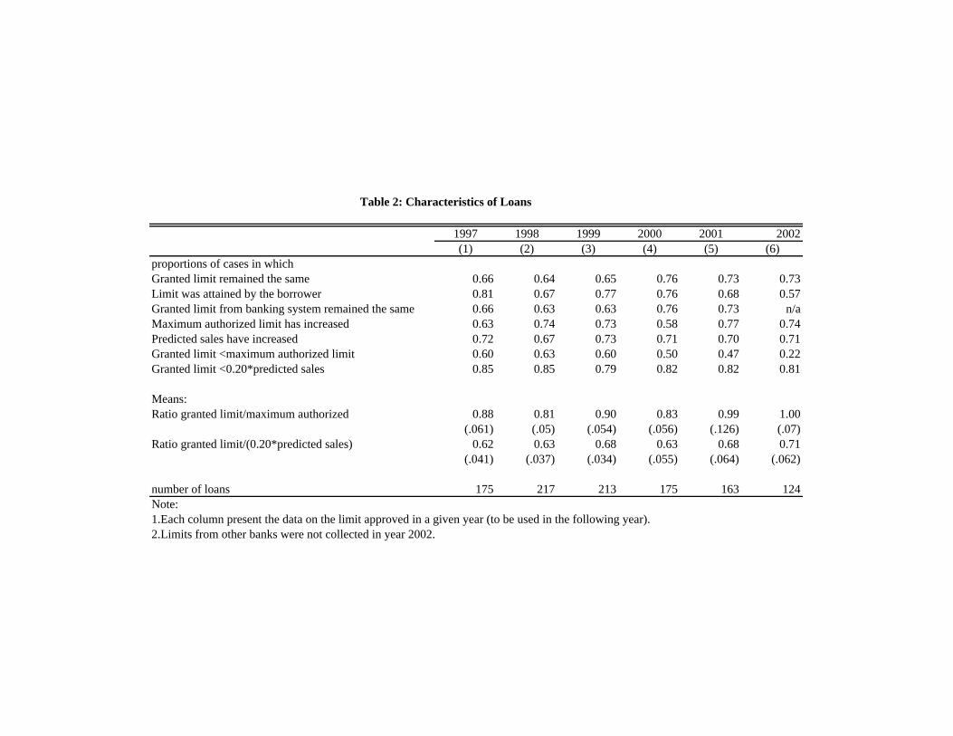
1997 1998 1999 2000 2001 2002(1) (2) (3) (4) (5) (6)

proportions of cases in whichGranted limit remained the same 0.66 0.64 0.65 0.76 0.73 0.73Limit was attained by the borrower 0.81 0.67 0.77 0.76 0.68 0.57Granted limit from banking system remained the same 0.66 0.63 0.63 0.76 0.73 n/aMaximum authorized limit has increased 0.63 0.74 0.73 0.58 0.77 0.74Predicted sales have increased 0.72 0.67 0.73 0.71 0.70 0.71Granted limit <maximum authorized limit 0.60 0.63 0.60 0.50 0.47 0.22Granted limit <0.20*predicted sales 0.85 0.85 0.79 0.82 0.82 0.81

Means:Ratio granted limit/maximum authorized 0.88 0.81 0.90 0.83 0.99 1.00

(.061) (.05) (.054) (.056) (.126) (.07)Ratio granted limit/(0.20*predicted sales) 0.62 0.63 0.68 0.63 0.68 0.71

(.041) (.037) (.034) (.055) (.064) (.062)

number of loans 175 217 213 175 163 124Note: 1.Each column present the data on the limit approved in a given year (to be used in the following year).2.Limits from other banks were not collected in year 2002.

Table 2: Characteristics of Loans

Mean of:Proportion limit was limit was log(current limit)

increased not changed -log(past limit) Client<=5 years Client>5 years(1) (2) (3) (4) (5) (6)

A- HAS PAST UTILIZATION REACHED MAXIMUM ?Yes 0.72 0.34 0.60 0.16 0.55 0.67No 0.28 0.30 0.66 0.12 0.61 0.71Difference 0.05 -0.05 0.03 -0.05 -0.04

(.054) (.056) (.04) (.081) (.072)B-HAVE PROJECTED SALES INCREASED?Yes 0.71 0.43 0.52 0.19 0.54 0.54No 0.29 0.25 0.61 0.06 0.50 0.67Difference 0.18 -0.09 0.13 0.04 -0.13

(.076) (.079) (.053) (.114) (.101)C-HAVE ACTUAL SALES INCREASED? Yes 0.71 0.33 0.62 0.13 0.61 0.68No 0.29 0.25 0.69 0.12 0.70 0.72Difference 0.08 -0.06 0.02 -0.09 -0.04

(.041) (.043) (.029) (.059) (.05)D-HAS PROFIT OVER SALE INCREASED? Yes 0.56 0.29 0.67 0.11 0.64 0.69No 0.44 0.35 0.61 0.16 0.61 0.69Difference -0.05 0.06 -0.05 0.03 0.00

(.042) (.044) (.028) (.059) (.053)E- HAS CURRENT RATIO INCREASED? Yes 0.53 0.32 0.62 0.12 0.61 0.70No 0.47 0.29 0.67 0.14 0.67 0.68Difference 0.03 -0.05 -0.02 -0.06 0.02

(.038) (.04) (.027) (.052) (.049)

Note: 1. Each panel divides the sample in two subsamples, according to the answer to the question asked in the panel title.2.Column 1 gives the proportion of the sample that falls into each categorie. The first two rows in Column 2 to 6 display the mean of the relevant variables in the subsample where the answer to the question in the panel title is yes (row 1 in each panel) , and no (row 2 in each panel).3.Row 3 is the difference between row 1 and 3 in each panel. The standard errors are in parenthese in row 4.

Proportion of cases wherelimit was changed

Propoportion of cases where

Table 3: Changes in working capital limits, by firm characteristics

1996-1997 1998-1999 2000-2002Firm's category

A. Average change in limitsmall 0.110 0.075 0.070

(.021) (.013) (.014)

medium 0.040 0.093 0.011(.032) (.030) (.025)

biggest 0.093 0.147 0.000(.064) (.040) (.031)

B. Proportion of cases where limit was not changedsmall 0.701 0.701 0.724

(.043) (.031) (.027)

medium 0.667 0.608 0.798(.088) (.055) (.040)

biggest 0.625 0.692 0.769(.183) (.075) (.053)

C. Average change in limit, conditional on changesmall 0.366 0.252 0.253

(.045) (.035) (.045)

medium 0.119 0.237 0.053(.093) (.068) (.124)

biggest 0.248 0.479 -0.002(.137) (.062) (.138)

Notes:1-The first row of each panel presentsthe average of log(working capital limit granted at date t)-log(working capital limit granted at date t-1).2-Standard errors in parentheses below the average.3-Number of observations in the third row of each panel.4-"Small firms" are firms with investment in plant and machinery below Rs 6.5 million ."Medium firms" are firms with investment in plant and machinery above Rs 6.5 million. and below Rs 10 million. "Biggest firms" are firms with investment in plant and machinery above Rs 10 million.

Years

Table 4: Average change in limit

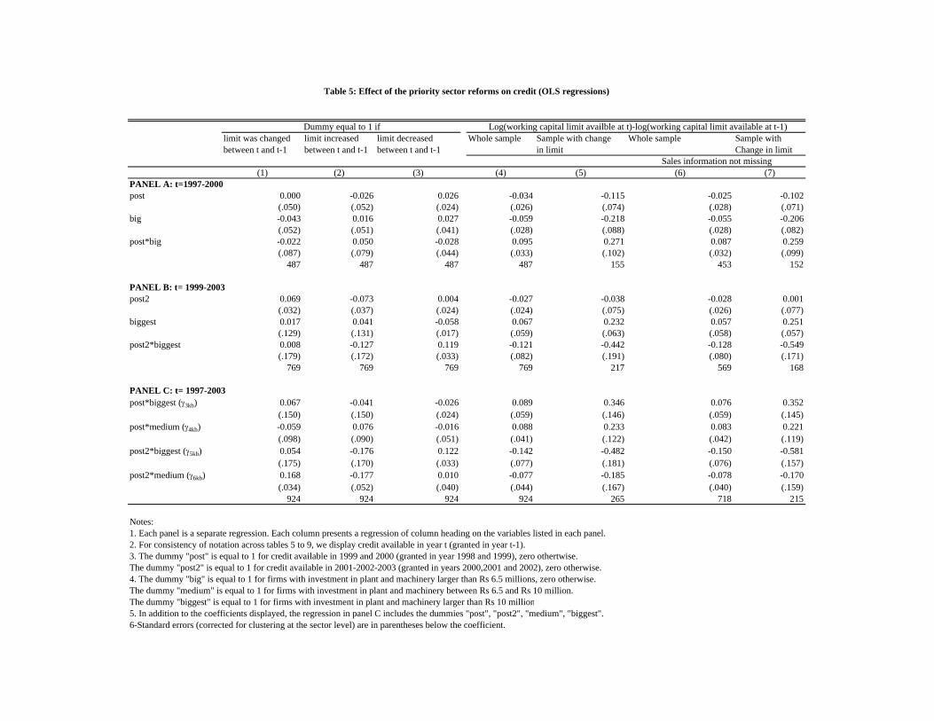
limit was changed limit increased limit decreased Whole sample Sample with change Whole sample Sample withbetween t and t-1 between t and t-1 between t and t-1 in limit Change in limit

(1) (2) (3) (4) (5) (6) (7)PANEL A: t=1997-2000post 0.000 -0.026 0.026 -0.034 -0.115 -0.025 -0.102

(.050) (.052) (.024) (.026) (.074) (.028) (.071)big -0.043 0.016 0.027 -0.059 -0.218 -0.055 -0.206

(.052) (.051) (.041) (.028) (.088) (.028) (.082)post*big -0.022 0.050 -0.028 0.095 0.271 0.087 0.259

(.087) (.079) (.044) (.033) (.102) (.032) (.099)487 487 487 487 155 453 152

PANEL B: t= 1999-2003post2 0.069 -0.073 0.004 -0.027 -0.038 -0.028 0.001

(.032) (.037) (.024) (.024) (.075) (.026) (.077)biggest 0.017 0.041 -0.058 0.067 0.232 0.057 0.251

(.129) (.131) (.017) (.059) (.063) (.058) (.057)post2*biggest 0.008 -0.127 0.119 -0.121 -0.442 -0.128 -0.549

(.179) (.172) (.033) (.082) (.191) (.080) (.171)769 769 769 769 217 569 168

PANEL C: t= 1997-2003post*biggest (γ3kb) 0.067 -0.041 -0.026 0.089 0.346 0.076 0.352

(.150) (.150) (.024) (.059) (.146) (.059) (.145)post*medium (γ4kb) -0.059 0.076 -0.016 0.088 0.233 0.083 0.221

(.098) (.090) (.051) (.041) (.122) (.042) (.119)post2*biggest (γ5kb) 0.054 -0.176 0.122 -0.142 -0.482 -0.150 -0.581

(.175) (.170) (.033) (.077) (.181) (.076) (.157)post2*medium (γ6kb) 0.168 -0.177 0.010 -0.077 -0.185 -0.078 -0.170

(.034) (.052) (.040) (.044) (.167) (.040) (.159)924 924 924 924 265 718 215

Notes:1. Each panel is a separate regression. Each column presents a regression of column heading on the variables listed in each panel.2. For consistency of notation across tables 5 to 9, we display credit available in year t (granted in year t-1).3. The dummy "post" is equal to 1 for credit available in 1999 and 2000 (granted in year 1998 and 1999), zero othertwise.The dummy "post2" is equal to 1 for credit available in 2001-2002-2003 (granted in years 2000,2001 and 2002), zero otherwise.4. The dummy "big" is equal to 1 for firms with investment in plant and machinery larger than Rs 6.5 millions, zero otherwise.The dummy "medium" is equal to 1 for firms with investment in plant and machinery between Rs 6.5 and Rs 10 million.The dummy "biggest" is equal to 1 for firms with investment in plant and machinery larger than Rs 10 million5. In addition to the coefficients displayed, the regression in panel C includes the dummies "post", "post2", "medium", "biggest".6-Standard errors (corrected for clustering at the sector level) are in parentheses below the coefficient.

Log(working capital limit availble at t)-log(working capital limit available at t-1)

Sales information not missing

Dummy equal to 1 if

Table 5: Effect of the priority sector reforms on credit (OLS regressions)

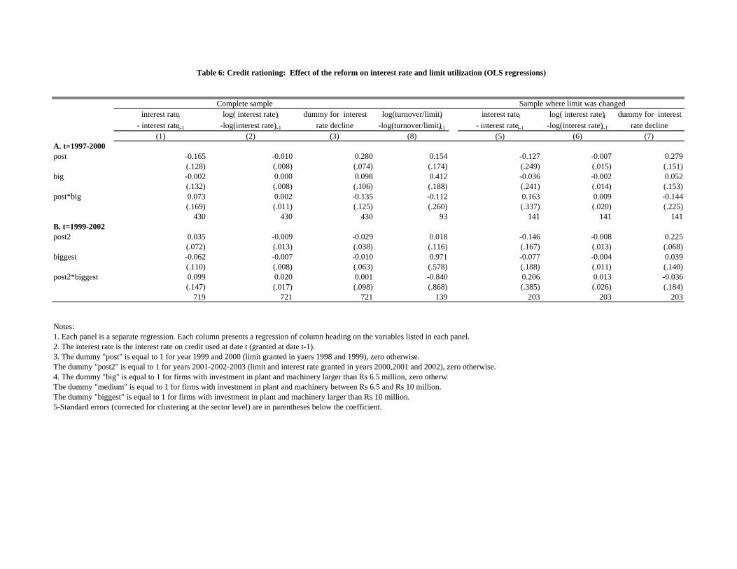
interest ratet log( interest rate)t dummy for interest log(turnover/limit)t interest ratet log( interest rate)t dummy for interest- interest ratet-1 -log(interest rate)t-1 rate decline -log(turnover/limit)t-1 - interest ratet-1 -log(interest rate)t-1 rate decline

(1) (2) (3) (8) (5) (6) (7)A. t=1997-2000post -0.165 -0.010 0.280 0.154 -0.127 -0.007 0.279

(.128) (.008) (.074) (.174) (.249) (.015) (.151)big -0.002 0.000 0.098 0.412 -0.036 -0.002 0.052

(.132) (.008) (.106) (.188) (.241) (.014) (.153)post*big 0.073 0.002 -0.135 -0.112 0.163 0.009 -0.144

(.169) (.011) (.125) (.260) (.337) (.020) (.225)430 430 430 93 141 141 141

B. t=1999-2002post2 0.035 -0.009 -0.029 0.018 -0.146 -0.008 0.225

(.072) (.013) (.038) (.116) (.167) (.013) (.068)biggest -0.062 -0.007 -0.010 0.971 -0.077 -0.004 0.039

(.110) (.008) (.063) (.578) (.188) (.011) (.140)post2*biggest 0.099 0.020 0.001 -0.840 0.206 0.013 -0.036

(.147) (.017) (.098) (.868) (.385) (.026) (.184)719 721 721 139 203 203 203

Notes:1. Each panel is a separate regression. Each column presents a regression of column heading on the variables listed in each panel.2. The interest rate is the interest rate on credit used at date t (granted at date t-1).3. The dummy "post" is equal to 1 for year 1999 and 2000 (limit granted in yaers 1998 and 1999), zero otherwise.The dummy "post2" is equal to 1 for years 2001-2002-2003 (limit and interest rate granted in years 2000,2001 and 2002), zero otherwise.4. The dummy "big" is equal to 1 for firms with investment in plant and machinery larger than Rs 6.5 million, zero otherwiThe dummy "medium" is equal to 1 for firms with investment in plant and machinery between Rs 6.5 and Rs 10 million.The dummy "biggest" is equal to 1 for firms with investment in plant and machinery larger than Rs 10 million.5-Standard errors (corrected for clustering at the sector level) are in parentheses below the coefficient.

Sample where limit was changed

Table 6: Credit rationing: Effect of the reform on interest rate and limit utilization (OLS regressions)

Complete sample

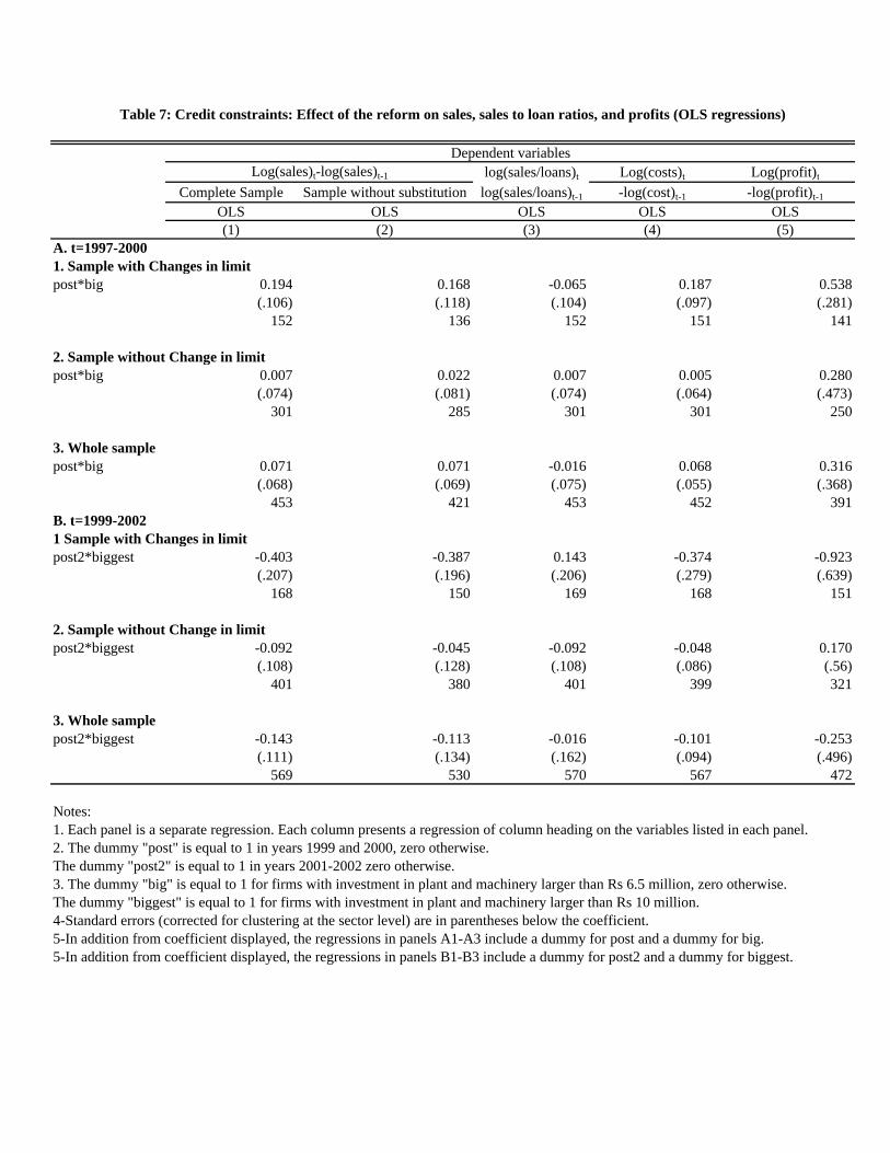
log(sales/loans)t Log(costs)t Log(profit)t

Complete Sample Sample without substitution log(sales/loans)t-1 -log(cost)t-1 -log(profit)t-1

OLS OLS OLS OLS OLS(1) (2) (3) (4) (5)

A. t=1997-20001. Sample with Changes in limitpost*big 0.194 0.168 -0.065 0.187 0.538

(.106) (.118) (.104) (.097) (.281)152 136 152 151 141

2. Sample without Change in limitpost*big 0.007 0.022 0.007 0.005 0.280

(.074) (.081) (.074) (.064) (.473)301 285 301 301 250

3. Whole samplepost*big 0.071 0.071 -0.016 0.068 0.316

(.068) (.069) (.075) (.055) (.368)453 421 453 452 391

B. t=1999-20021 Sample with Changes in limitpost2*biggest -0.403 -0.387 0.143 -0.374 -0.923

(.207) (.196) (.206) (.279) (.639)168 150 169 168 151

2. Sample without Change in limitpost2*biggest -0.092 -0.045 -0.092 -0.048 0.170

(.108) (.128) (.108) (.086) (.56)401 380 401 399 321

3. Whole samplepost2*biggest -0.143 -0.113 -0.016 -0.101 -0.253

(.111) (.134) (.162) (.094) (.496)569 530 570 567 472

Notes:1. Each panel is a separate regression. Each column presents a regression of column heading on the variables listed in each panel.2. The dummy "post" is equal to 1 in years 1999 and 2000, zero otherwise.The dummy "post2" is equal to 1 in years 2001-2002 zero otherwise.3. The dummy "big" is equal to 1 for firms with investment in plant and machinery larger than Rs 6.5 million, zero otherwise.The dummy "biggest" is equal to 1 for firms with investment in plant and machinery larger than Rs 10 million.4-Standard errors (corrected for clustering at the sector level) are in parentheses below the coefficient. 5-In addition from coefficient displayed, the regressions in panels A1-A3 include a dummy for post and a dummy for big.5-In addition from coefficient displayed, the regressions in panels B1-B3 include a dummy for post2 and a dummy for biggest.

Table 7: Credit constraints: Effect of the reform on sales, sales to loan ratios, and profits (OLS regressions)

Dependent variablesLog(sales)t-log(sales)t-1

log(sales/loans)t Log(costs)t

Complete Sample Sample without substitution log(sales/loans)t-1 -log(cost)t-1

(1) (2) (3) (4)

post*big (γ3y) 0.238 0.235 -0.114 0.205(.153) (.162) (.256) (.151)

post*medium (γ4y) 0.160 0.122 0.000 0.165(.118) (.13) (.106) (.105)

post2*big (γ5y) -0.421 -0.400 0.156 -0.384(.197) (.186) (.204) (.279)

post2*med (γ6y) -0.074 -0.080 -0.139 -0.058(.112) (.114) (.202) (.105)

215 193 216 215

ratio 1: γ3y/γ3kb 0.676 0.666 -0.324 0.583

ratio 2: γ4y/γ4kb 0.725 0.555 -0.001 0.749

ratio 3: γ5y/γ5kb 0.725 0.689 -0.269 0.660

ratio 4: γ6y/γ6kb 0.439 0.470 0.820 0.340

test ratio 1=ratio2 0.39 0.46 0.388 0.38(p value) (0.53) (0.50) (0.53) (0.54)

test ratio 1=ratio2=ratio3 0.20 0.28 0.20 0.19(p value) (0.82) (0.75) (0.81) (0.83)

test ratio 1=ratio2=ratio3=ratio4 0.16 0.21 0.16 0.13(p value) (0.92) (0.89) (0.92) (0.94)

Notes:1.All the regressions are estimated in the sample were the limit was changed.2. The dummy "post" is equal to 1 in years 1999 and 2000, zero otherwise.The dummy "post2" is equal to 1 in years 2001-2002 zero otherwise.3. The dummy "big" is equal to 1 for firms with investment in plant and machinery larger than Rs 6.5 millions, zero otherwise.The dummy "biggest" is equal to 1 for firms with investment in plant and machinery larger than Rs 10 million.4-Standard errors (corrected for clustering at the sector level) are in parentheses below the coefficient. 5-In addition from coefficient displayed, the regressions include dummies for post, post2, medium, and biggest.6-The parameters in parenthesis refer to equation (6) in the text. The ratios are computed using the parameters of equation (5)in the text, displayed in column 7 and panel C of table 5

Table 8: Credit constraints: Effect of the reform on sales and cost and overidentification tests

Log(sales)t-log(sales)t-1

Dependent variables

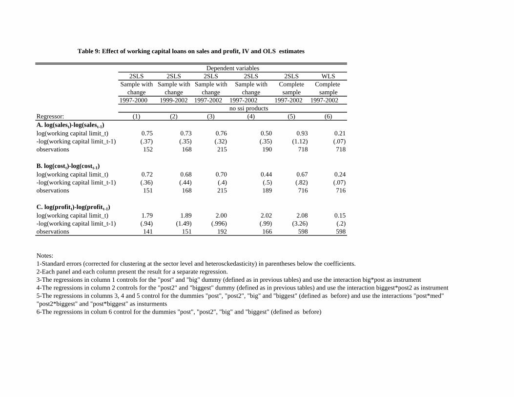
2SLS 2SLS 2SLS 2SLS 2SLS WLSSample with Sample with Sample with Sample with Complete Complete

change change change change sample sample1997-2000 1999-2002 1997-2002 1997-2002 1997-2002 1997-2002

no ssi productsRegressor: (1) (2) (3) (4) (5) (6)A. log(salest)-log(salest-1)log(working capital limit_t) 0.75 0.73 0.76 0.50 0.93 0.21-log(working capital limit_t-1) (.37) (.35) (.32) (.35) (1.12) (.07)observations 152 168 215 190 718 718

B. log(costt)-log(costt-1)log(working capital limit_t) 0.72 0.68 0.70 0.44 0.67 0.24-log(working capital limit_t-1) (.36) (.44) (.4) (.5) (.82) (.07)observations 151 168 215 189 716 716

C. log(profitt)-log(profitt-1)log(working capital limit_t) 1.79 1.89 2.00 2.02 2.08 0.15-log(working capital limit_t-1) (.94) (1.49) (.996) (.99) (3.26) (.2)observations 141 151 192 166 598 598

Notes: 1-Standard errors (corrected for clustering at the sector level and heterosckedasticity) in parentheses below the coefficients.2-Each panel and each column present the result for a separate regression.3-The regressions in column 1 controls for the "post" and "big" dummy (defined as in previous tables) and use the interaction big*post as instrument4-The regressions in column 2 controls for the "post2" and "biggest" dummy (defined as in previous tables) and use the interaction biggest*post2 as instrument5-The regressions in columns 3, 4 and 5 control for the dummies "post", "post2", "big" and "biggest" (defined as before) and use the interactions "post*med""post2*biggest" and "post*biggest" as insturments6-The regressions in colum 6 control for the dummies "post", "post2", "big" and "biggest" (defined as before)

Table 9: Effect of working capital loans on sales and profit, IV and OLS estimates

Dependent variables