HAL Id: halshs-01713068https://halshs.archives-ouvertes.fr/halshs-01713068v5

Preprint submitted on 11 Oct 2021

HAL is a multi-disciplinary open accessarchive for the deposit and dissemination of sci-entific research documents, whether they are pub-lished or not. The documents may come fromteaching and research institutions in France orabroad, or from public or private research centers.

L’archive ouverte pluridisciplinaire HAL, estdestinée au dépôt et à la diffusion de documentsscientifiques de niveau recherche, publiés ou non,émanant des établissements d’enseignement et derecherche français ou étrangers, des laboratoirespublics ou privés.

Do Female Role Models Reduce the Gender Gap inScience? Evidence from French High Schools

Thomas Breda, Julien Grenet, Marion Monnet, Clémentine van Effenterre

To cite this version:Thomas Breda, Julien Grenet, Marion Monnet, Clémentine van Effenterre. Do Female Role ModelsReduce the Gender Gap in Science? Evidence from French High Schools. 2021. �halshs-01713068v5�

WORKING PAPER N° 2018 – 06

Do Female Role Models Reduce the Gender Gap in Science? Evidence from French High Schools

Thomas Breda Julien Grenet

Marion Monnet Clémentine Van Effenterre

JEL Codes: C93, I24, J16. Keywords: Role Models; Gender Gap; STEM; Stereotypes; Choice of Study.

Do Female Role Models Reduce the Gender Gap inScience? Evidence from French High Schools∗

Thomas BredaJulien GrenetMarion Monnet

Clémentine Van Effenterre

First version: January 2018This version: October 2021

Abstract

We show in a large-scale field experiment that a brief exposure to female role models workingin scientific fields affects high school students’ perceptions and choice of undergraduatemajor. While the classroom interventions generally reduce the prevalence of stereotypicalviews on jobs in science and gender differences in abilities, the effects on educationalchoices are concentrated among high-achieving girls in Grade 12. They are more likelyto enroll in selective and male-dominated STEM programs in college. The most effectiverole model interventions are those that improved students’ perceptions of STEM careerswithout overemphasizing women’s underrepresentation in science.

JEL codes: C93, I24, J16Keywords: Role Models; Gender Gap; STEM ; Stereotypes; Choice of Study.

∗Breda: CNRS, Paris School of Economics, 48 boulevard Jourdan, 75014, Paris, France (e-mail: thomas.breda@ens.fr); Grenet:CNRS, Paris School of Economics, 48 boulevard Jourdan, 75014, Paris, France (e-mail: julien.grenet@psemail.eu); Monnet: InstitutNational d’Études Démographiques, 9 cours des Humanités, 93300, Aubervilliers, France (e-mail: marion.monnet@ined.fr); Van Ef-fenterre: University of Toronto, 150 St. George Street, Toronto, Ontario M5S3G7, Canada (e-mail: c.vaneffenterre@utoronto.ca).We are grateful to the staff at the L’Oréal Foundation, especially Diane Baras, Aude Desanges, Margaret Johnston-Clarke, SalimaMaloufi-Talhi, David McDonald, and Elisa Simonpietri for their continued support to this project. We also thank the staff atthe French Ministry of Education (Ministère de l’Éducation Nationale, Direction de l’Évaluation, de la Prospective et de la Perfor-mance) and at the Rectorats of Créteil, Paris, and Versailles for their invaluable assistance in collecting the data. This paper greatlybenefited from discussions and helpful comments from Marcella Alsan, Iris Bohnet, Scott Carrell, Clément de Chaisemartin, BrunoCrépon, Esther Duflo, Lena Edlund, Ruth Fortmann, Pauline Givord, Laurent Gobillon, Marc Gurgand, Élise Huillery, Philip Ketz,Sandra McNally, Amanda Pallais, and Liam Wren-Lewis. We thank participants at the ASSA/AEA Annual Meeting in Atlanta,CEPR/IZA Annual Symposium in Labor Economics 2018 in Paris, EALE 2018 in Lyon, EEA-ESEM 2018 in Cologne, GenderEconomics Workshop 2018 in Berlin, Gender and Tech Conference at Harvard, IWAEE Conference in Catanzaro, and JournéesLAGV 2018 in Aix-Marseille. We also thank seminar participants at Bristol, DEPP, LSE, Harvard Kennedy School, HEC Lausanne,Maastrict SBE, OECD EDU Forum, PSE, Stockholm University SOFI, and Université Paris 8. We are grateful to the Institutdes politiques publiques (IPP) for continuous support and to Sophie Cottet for her assistance in contacting schools. Financialsupport for this study was received from the Fondation L’Oréal, from the Institut des Politiques Publiques, and from the EURgrant ANR-17-EURE-0001. The project received IRB approval at J-PAL Europe and was registered in the AEA RCT Registrywith ID AEARCTR-0000903.

1

Introduction

Women’s increasing participation in science and engineering in the U.S. has leveled off in thepast decade (National Science Foundation, 2017). This trend, which is common to almost allOECD countries, is a source of concern for two main reasons. First, it exacerbates genderinequality in the labor market, as Science, Technology, Engineering, and Mathematics (STEM)occupations offer higher average salaries (Brown and Corcoran, 1997; Black et al., 2008; Blauand Kahn, 2017) and show a smaller gender wage gap (Beede et al., 2011). Second, in acontext of heightened concern over a shortage of STEM workers in the advanced economies, thistrend is likely to represent a worsening loss of talent that could reduce aggregate productivity(Weinberger, 1999; Hoogendoorn et al., 2013).

The underrepresentation of women in these traditionally male-dominated fields can alsoconstitute a self-fulfilling prophecy for subsequent generations, as girls have little opportunityto interact with women working in these fields and who could inspire them. A large literaturehas established that exposing female students to successful or admirable women can help breakthis vicious circle. Most of the existing papers focus on potential role models that interact on aregular basis with the individuals they may influence, such as teachers or instructors (Bettingerand Long, 2005; Carrell et al., 2010), university advisors (Canaan and Mouganie, forthcoming),or doctors (Riise et al., forthcoming). Recently, two studies have shown that a one-off exposureto external female role models can also have large effects on female representation in male-dominated fields of study. Porter and Serra (2020) document a positive impact of two femalerole models who were carefully selected among the economics alumni of Southern MethodistUniversity in the U.S. on the likelihood of female students majoring in economics. Del Carpioand Guadalupe (2018) demonstrate the effectiveness, relative to other types of interventions,of virtual role models to reduce identity costs related to female participation in STEM andto foster female applications to a software-coding program.1 An attractive feature of theselight-touch interventions for identifying role model effects is that they remove the influences ofpotential confounding factors such as gender differences in teaching practices (Lavy and Sand,2018; Terrier, 2020; Carlana, 2019)

Although the literature provides compelling evidence that external role models have sizeableeffects on educational choices, little is known about how these effects are transmitted. Rolemodels could directly affect students’ preferences. They might change their expectations bymodifying their beliefs. By providing an inspirational and relatable model, they could also

1Related studies outside the context of STEM education include field experiments on exposure to women inleadership positions in India (Beaman et al., 2012) and the provision of information on the returns to educationby role models of poor or rich background in Madagascar (Nguyen, 2008).

2

counteract the effects of gender norms on students’ social identity (Gladstone and Cimpian,2020). Which of those channels are most affected by external role models? To what extentdo changes in students’ perceptions translate into changes in educational choices? Are all rolemodels equally able to influence students’ decision making?

This paper’s contributes to answering these questions by analyzing the effects of a one-hourin-class exposure to external female scientists on female representation in STEM fields of study,and by investigating how the effectiveness of such interventions depends on the characteristicsof the role models and the messages they convey. We use a large-scale randomized experimentcombined with a comprehensive post-intervention survey to directly measure how role modelsaffect students’ perceptions, beliefs, and enrollment outcomes. Compared to previous studies, astrength of our research design is to involve a large number of role model participants—56 intotal. We leverage the diversity of these women’s profiles to better understand what makes anefficient role model. Building on the rapidly expanding literature on the use of machine learningto analyze treatment effect heterogeneity (Athey and Imbens, 2016, 2017; Mullainathan andSpiess, 2017; Wager and Athey, 2018; Chernozhukov et al., 2018), we propose a novel empiricalapproach that relates the treatment effects on STEM enrollment outcomes to the treatmenteffects on potential channels. This constitutes a methodological contribution that can be usedto investigate mechanisms in randomized controlled trials.

The program we evaluate is called “For Girls in Science” (Pour les Filles et la Science)and was launched in 2014 by the L’Oréal Foundation—the corporate foundation of the world’sleading cosmetics manufacturer—to encourage girls to explore STEM career paths. It consists ofone-hour in-class interventions by women with two very distinct profiles: half are young scientists(either Ph.D. candidates or postdoctoral researchers) who were awarded the L’Oréal-UNESCO“For Women in Science” Fellowship; the others are young professionals privately employed asscientists in the Research and Innovation division of the L’Oréal group. In the main part of theintervention, the role models share their experience and career path with the students. Theyalso provide information on science-related careers in general and on gender stereotypes usingtwo short videos.

The evaluation was conducted during the 2015/16 academic year in 98 high schools locatedin the Paris region. It involved 19,451 students from Grade 10 and Grade 12 (science track),two grade levels at the end of which irreversible educational choices are made by students. Halfof the classes were randomly selected to be visited by one of the 56 role model participants, whowere assigned to those classes through a registration process on a first-come, first-served basis.

We show that the role models’ interventions led to a significant increase in the share ofgirls enrolling in STEM fields, but only in the educational tracks where they are stronglyunderrepresented. In Grade 10, the classroom visits had no detectable impact on boys’ and

3

girls’ probability of enrolling in the science track in Grade 11, where girls are only slightlyunderrepresented (47 percent of students). By contrast, the intervention induced a significant2.4-percentage-point increase in STEM undergraduate enrollment among girls in Grade 12, or anincrease of 8 percent over the baseline rate of 29 percent, while the effect for boys was negligible.This positive impact on female STEM enrollment is driven by high-achieving female studentsshifting to selective STEM programs, which lead to the most prestigious graduate schools, andmale-dominated STEM programs (math, physics, computer science, and engineering). Theseresults constitute the first field evidence that in-person exposure to external female role modelsaffects STEM enrollment decisions at college entry. They complement the findings from previousresearch on the effects of external role models on female representation in economics majors(Porter and Serra, 2020), and of female teachers (e.g., Carrell et al., 2010) and virtual rolemodels (Del Carpio and Guadalupe, 2018) in STEM.

To explore the channels through which role models affect students’ enrollment outcomes, weconducted a post-treatment student survey consisting of an eight-page questionnaire administeredin class one to six months after the classroom interventions. We also collected administrativedata on high school graduation exams (Baccalauréat) at the end of Grade 12. Our results showthat the role model interventions significantly improved students’ perceptions of science-relatedjobs at both grade levels, with no indication of declining effects over a period of up to six months.For girls in Grade 12, the interventions significantly increased aspirations for science-relatedcareers. They also helped mitigate some of the stereotypes typically associated with STEMoccupations (such as being hard to reconcile with family life) and heightened the perceptionthat these jobs pay better. By contrast, the intervention had no significant effect on students’self-reported taste for science subjects or their academic performance, and only slightly increasedtheir math self-concept at both grade levels.

One of the most interesting—and least expected—findings concerns the effects on students’perceptions of gender roles in science. The classroom interventions not only were effective indebiasing students’ beliefs about gender differences in math aptitude, they also raised awarenessof the underrepresentation of women in science. The combination of these two effects triggeredan unintended ex-post rationalization by students of the gender imbalance in scientific fields andoccupations, making them more likely to agree with the statement that women dislike scienceand that they face discrimination in science-related jobs. Explicitly correcting self-stereotypingbeliefs (Coffman, 2014) and misperceptions about women’s representation in science (Bursztynand Yang, 2021) thus appears to have generated more ambiguous perceptions among studentsthan the intervention’s gender-neutral messages about jobs and careers.

Building on the method proposed by Chernozhukov et al. (2018), we develop a novel approachto relate the student-level treatment effects on enrolment outcomes to the treatment effects on

4

potential channels. Our results show that the interventions that had the greatest impact onfemale enrollment in selective STEM programs are those that most improved girls’ perceptionsof science-related careers without reinforcing the perception that women are underrepresentedin science. By contrast, we find that the role models’ ability to steer girls towards selectiveSTEM programs is essentially uncorrelated with their effects on students’ perceptions of genderdifferences in aptitude for science.

Overall, our exploration of the different channels provides consistent evidence that theemphasis on gender issues is less important to the effectiveness of such interventions than theability of role models to project a positive and inclusive image of science-related careers, thusembodying an attractive, attainable path to them.

Finally, we highlight the importance of the role model component of the intervention. First,we argue that the provision of general information on STEM careers cannot explain alone theeffects of the interventions on enrollment outcomes. To test the sensitivity of students’ attitudesand choices to the intensity of the information component of the treatment, we provided 36 ofthe 56 role models with a set of slides that contained twice as much informational contentas the standard set, including information about wages and employment conditions in STEMjobs. We find no evidence that the treatment effects on students’ choice of college major differsignificantly between the two sets of slides. Second, we document a high degree of heterogeneityin treatment effects according to the role models’ professional background. Those employed bythe sponsoring firm had a significantly greater effect on girls’ probability of enrolling in selectiveSTEM programs than the young researchers, despite being exposed to students with similarobservable characteristics. Although the two groups were equally effective in debunking thestereotype on gender differences in math aptitude, we find clear evidence that those with aprofessional background were better able to improve girls’ perceptions of science-related jobs andraise their aspirations for such careers. Conversely, they were less likely to reinforce students’belief that women are underrepresented in science. Together, these results show that role modelinterventions are not reducible to the provision of standardized information and that female rolemodels are not interchangeable. They confirm, in a real-life setting, results from lab experimentsin social psychology highlighting the importance of role models’ profiles (Lockwood and Kunda,1997; Cheryan et al., 2011; Betz and Sekaquaptewa, 2012; O’Brien et al., 2016).

The remainder of the paper is organized as follows. Section 1 provides institutional back-ground on the French educational system and the gender gap in STEM fields. Section 2 describesthe intervention and the experimental design. Section 3 presents the data and empirical strategy.Section 4 analyzes the effects of role model interventions on student perceptions, self-concept, andeducational outcomes. Section 5 extends the analysis to the role of information, the persistenceof effects, and potential spillovers. Section 6 discusses mechanisms and Section 7 concludes.

5

1 Institutional Background

1.1 Structure of the French Education System

In France, education is compulsory from the age of 6 to the age of 16, with the academicyear running from September to June. The school system consists of five years of elementaryeducation (Grades 1 to 5) and seven years of secondary education, divided into four years ofmiddle school (collège, Grades 6 to 9) and three of high school (lycée, Grades 10 to 12). Studentscomplete high school with the Baccalauréat national exam, which they must pass for admissionto higher education.

High school tracks. The tracking of students occurs at two critical stages (see Figure 1). Atthe end of middle school, about two-thirds of students are admitted to general and technologicalupper secondary education (Seconde générale et technologique) and the remaining third aretracked into vocational schools (Seconde professionnelle). After the first year of high school(Grade 10), the general and technological track is further split: approximately 80 percent of thestudents are directed to the general Baccalauréat program for the last two years of high school(Grades 11 and 12), while the remaining 20 percent, who are mostly low-achieving students,are directed towards a technological Baccalauréat, which is more geared towards the needs ofbusiness and industry and leads to shorter studies.

In the Spring term of Grade 10, the students who have been allowed to pursue the generaltrack are required to choose among three sub-tracks in Grade 11: Science (Première S),Humanities (Première L), and Social sciences (Première ES). This is an important choice, giventhat the curriculum and high school examinations are specific to each Baccalauréat track andthus directly impact students’ educational opportunities and career prospects. It is almostimpossible, for instance, for a student to be admitted to engineering or medical undergraduateprograms without a Baccalauréat in science. Students directed to the technological track afterGrade 10 are also required to choose among eight possible STEM and non-STEM sub-tracks,which will affect their choice of field of study in higher education.

College entry. In the Spring term of Grade 12, students in their final year of high school applyfor admission to higher education programs through a centralized online admission platform. Theprograms to which students can apply fall into two broad categories, each accounting for abouthalf of first-year undergraduate enrollment: (i) non-selective undergraduate university programs(Licence), which are open to all students who hold the Baccalauréat; and (ii) selective programs,which can select students based on their academic achievement. Both types of programs offer

6

specializations in STEM and non-STEM fields. Among selective programs, the most prestigiousare the two-year Classes préparatoires aux Grandes Écoles (CPGE), which prepare students totake the national entry exams to elite graduate schools (Grandes Écoles). These programs arespecialized either in science, in economics and business or in humanities. Within the scienceCPGE programs, the main fields of specialization are mathematics and physics (MPSI), physicsand chemistry (PCSI), and biology/geoscience (BCPST). The other selective undergraduateprograms (Section de technicien supérieur or STS) are mostly targeted to students holding avocational or technological Baccalauréat and prepare for technical/vocational bachelor’s degrees.

1.2 Female Underrepresentation in STEM

In France, the share of female students in STEM-oriented studies starts to decline after Grade 10and drops sharply at entry into higher education. While 54 percent of the students in the generaland technological track in Grade 10 are girls, the share falls to 47 percent in the general sciencetrack (Grades 11 and 12) and further to 30 percent in the first year of higher education.2 Femaleunderrepresentation in STEM fields of study is more pronounced in the selective undergraduateprograms (shares of 18 percent in STS and 30 percent in CPGE) than in the non-selectiveprograms (35 percent). These proportions, which are computed from administrative data for2016/17, are almost identical to those of a decade earlier. Within STEM fields of study, femalestudents tend to specialize in earth and life sciences (female share: 62 percent) rather thanmathematics, physics, or computer science (female share: 26 percent).

The underrepresentation of women in STEM fields accounts for a good part of the genderpay gap among college graduates in France. Using a variety of administrative and surveydata sources, we show in Appendix A that across all majors, male graduates who obtained amaster’s degree in 2015 or 2016 earn a median gross annual starting salary of 32,122 euros,compared to 28,411 euros for female graduates. This amounts to an overall gap of 3,711 eurosper year, or 11.6 percent of men’s pay (see Table A1). Using standard decomposition methods,we find that the underrepresentation of female students in STEM accounts for approximately25 percent of this gap (see Table A2). Additionally, almost half of the 9.1 percent gender paygap within STEM can be ascribed to the fact that female graduates are less likely than malesto be enrolled in the selective and male-dominated fields, which lead to the best-paying degrees.These figures strongly suggest that in the French context, increasing the share of female studentsin STEM—especially in selective and male-dominated programs—would narrow the gender paygap substantially.

2At the high school level, the gender imbalance in STEM is more severe in the technological track (femaleshare: 17 percent) than in the general science track (female share: 47 percent).

7

2 Program and Experimental Design

2.1 The “For Girls in Science” Program

The “For Girls in Science” (FGiS) program is an awareness campaign launched in 2014 by theL’Oréal Foundation to encourage girls to explore STEM career paths. It consists of one-hour one-off classroom interventions by female role models with a background in science. The interventions,which take place in the presence of all students in the class, including boys, are carried outby female role models of two distinct types: (i) Ph.D. candidates or postdoctoral researcherswho have been awarded a fellowship by the L’Oréal Foundation (the L’Oréal-UNESCO “ForWomen in Science” Fellowship) and who participate in the program as part of their contract;and (ii) young professionals employed as scientists in the Research and Innovation division ofthe L’Oréal group who volunteer for the program.

Structure and content of the interventions. The classroom interventions last one hourand are divided into four main sequences. Each role model was provided with a set of slides as asupport for the entire in-class conversation. During the first sequence, a small number of slideshighlight two facts: (1) the labor market is marked by high demand for STEM skills and thereis a shortage of graduates in the relevant fields of study; and (2) women are underrepresentedin STEM careers. To investigate the role of information provision, we provided 36 of the56 role models with additional slides that they were free to use during this sequence. Theseslides contained supplementary information about average earnings and employment conditionsin STEM jobs, and were illustrated with examples of career prospects in humanities versusscience. In Section 5, we discuss the sensitivity of our results to this more intensive provision ofstandardized information.

The second sequence kicks off with two three-minute videos designed to illustrate anddeconstruct stereotypes about science-related careers and gender roles in science.3 The firstvideo, entitled “Science, Beliefs or Reality?,” uses interviews with high school students to debunkmyths about careers in science (e.g., jobs in science are more challenging, they necessarilyrequire long studies), stereotypes about scientists (e.g., they are introverted, lonely), and genderdifferences in science aptitude (e.g., women are naturally less talented in math). The secondvideo, entitled “Are we all Equal in Science?,” describes the common gender stereotypes aboutaptitude for science while providing information on brain plasticity and on how interactions andthe social environment shape men’s and women’s abilities and tastes. This sequence aims atstimulating class discussion based on students’ reactions to the videos.

3Screenshots of the two videos shown during the classroom interventions are displayed in Appendix Figure B1.

8

The third sequence centers on the female role model’s own experience as a woman witha background in science and consists of an interactive question-and-answer session with thestudents.4 Topics addressed during this discussion include the role model’s typical day at work,what she enjoys about her job, the biggest challenge she had to overcome, how she views herprofessional future, her everyday interactions with co-workers, how much she earns, and herwork-family balance. Consistent with the program’s emphasis on the role model dimension,this sequence was intended to be the longest and most important part of the intervention. Inorder to convey this objective to the role models, a full-day training was organized to helpthem share their experience with the students. The training also included a workshop onthe underrepresentation of women in science and a practice session aimed at enhancing oralcommunication skills.

The intervention concludes with an overview of the diversity of STEM studies and careers,illustrated by concrete examples such as jobs in graphic design, environmental engineering, andcomputer science.

2.2 Experimental Design

Selection of schools and classes. The evaluation was conducted in the three educationdistricts (académies) of the Paris region (Paris, Créteil, and Versailles) during the 2015/16academic year. Créteil and Versailles are the two largest education districts in France and thethree districts combined include 318,000 high school students in the general and technologicaltrack, or 20 percent of all French high school enrollment.

Figure 2 provides a detailed timeline of the evaluation. In the spring of 2015, the FrenchMinistry for Education agreed to support a randomized evaluation of the program and designatedone representative for each district as intermediary between the schools and the evaluationteam. In June, official letters informed high school principals that they were likely to becontacted to take part in the evaluation. All public and private high schools with at least fourclasses in Grade 10 and two in Grade 12 (science track) were contacted by our team betweenSeptember and December 2015, accounting for 349 of the 489 high schools operating in the threedistricts. Of these schools, 98 agreed to take part in the experiment, representing 28 percent ofGrade 10 enrollment and 29 percent of Grade 12 (science track) enrollment in the three districtscombined.5 The participating schools tend to be larger and are less likely to be private or tooperate in the Paris education district than the non-participating ones (see Appendix Table E1).Despite these differences, the experimental sample, which consists of 19,451 students (13,700 inGrade 10 and 5,751 in Grade 12), closely resembles the relevant student population, both in

4Screenshots of the slides used during the discussion are displayed in Appendix Figure B2.5The location of the participating schools is shown in Appendix Figure B3.

9

social composition and in average academic performance (see Appendix Table E2).

Randomization. In the fall of the 2015/16 school year, the principals were invited to selectat least six classes—four or more in Grade 10 and two or more in Grade 12 (science track)—andto indicate a preferred time slot and day for the interventions.6 In each school, half of the classesselected by the principal (up to the nearest integer) were randomly assigned to the treatmentgroup (302 classes in total) and the other half to the control group (299 classes). Table 1indicates that the random assignment successfully balanced the characteristics of students inthe treatment and control groups.

Role models. The experiment involved 56 female role models, of whom 35 were L’Oréalemployees and 21 were Ph.D. candidates or postdoctoral researchers. Table 2 provides summarystatistics of their characteristics. The researchers tend to be younger (30 vs. 36 years of age onaverage) and are less often of foreign nationality (10 vs. 17 percent). Although both types havevery high levels of educational attainment, 39 percent having graduated from a Grande École,the researchers are more likely than the professionals to hold (or prepare for) a Ph.D. (100 vs.38 percent) and to hold a degree in math, physics and engineering (38 vs. 14 percent). They arealso less likely to have children (19 vs. 58 percent) and to have been involved in the programin the previous year (19 vs. 29 percent). The professionals working at L’Oréal are employedin various activities: chemistry (development of new technologies for skin products), logisticsand supply chain management, statistics (consumer evaluation), immunology and toxicology.Although we could not collect direct information on earnings for reasons of confidentiality, weestimate based on aggregate information provided by the L’Oréal Group that the annual grosswages of these young professionals is between 45,000 and 65,000 euros, compared to between22,000 and 50,000 euros for the researchers. On average, each role model carried out fiveclassroom interventions in two different high schools.

Classroom interventions. The classroom visits took place between November 17, 2015, andMarch 3, 2016.7 The role models were asked to select two or three schools in which to carryout an average of three classroom visits per school—in most cases, two in Grade 10 and one inGrade 12. They were not assigned to the schools randomly but registered for the visits and timeslots during four registration sessions using an online system on a first-come, first-served basis.Randomly assigning the role models to the schools was not a feasible option, since most wereparticipating on a voluntary basis and during regular working hours. We therefore identify the

6In the vast majority of schools, principals selected exactly four Grade 10 and two Grade 12 classes.717 percent of the visits took place in November, 26 percent in December, 39 percent in January, 17 percent

in February, and 1 percent in March.

10

causal impact of role models in a setting where they have some freedom to choose the schoolsin which they intervene. The assignment process, however, did not involve any coordinationbetween the participants and was designed to limit their ability to select the schools they wouldvisit, as each registration session only concerned a subset of the participating schools.8

3 Data and Empirical Strategy

3.1 Data

To evaluate the program’s effects on student perceptions and educational choices, we combinethree main data sources: (i) a post-intervention survey of role models; (ii) a post-interventionsurvey of students; and (iii) student-level administrative data.9

Role model survey. After each visit to a school, the role models were invited to complete anonline survey. Besides collecting general feedback, this survey served to monitor compliance withrandom assignment, asking them to indicate each of the classes they visited. Summary statisticsare reported in Appendix Table E3. The interventions almost always (89 percent) took placein the presence of the teacher and sometimes (35 percent) of another adult. The role modelsreported organizational problems for only 16 percent of the visits (e.g. the intervention startedlate, the slides could not be shown). According to the survey, researchers and professionalswere equally likely to cover the intended topics, such as “jobs in science are fulfilling”, “theyare for girls too”, and “they pay well”. Finally, when asked about their overall perceptionof their classroom interventions, 93 percent said they went “well” (37 percent) or “very well”(56 percent). Students were generally perceived to be responsive to the key messages.

Student survey. We conducted a paper-and-pencil student survey in classes assigned to thetreatment and control groups one to six months after the classroom visits, between January andMay 2016. Each questionnaire was assigned a unique identifier so that it could be linked withstudent-level administrative data. The survey was designed to collect a rich set of informationon students’ preferences, beliefs and perceptions regarding science, self-concept and aspirations,and was administered in exam conditions under the supervision of a teacher. It was presentedas a general survey on students’ attitudes about science and science-related careers so as tominimize the risk that students would associate it with the FGiS program. It was eight pageslong and took about half an hour to complete.

8The role models were contacted four times to complete the schedule, on October 21, November 24, December 7,2015, and February 3, 2016.

9Translated versions of the two surveys are available online at https://mycore.core-cloud.net/index.php/s/L0aB9Kvpbot7sNh.

11

The survey items investigate the effects of classroom interventions on students’ perceptionsalong five dimensions: (i) general perceptions of science-related careers; (ii) perceptions of genderroles in science; (iii) taste for science subjects; (iv) math self-concept; and (v) science-relatedcareer aspirations. When conceptually related, we combine the survey items to construct asynthetic index for each dimension using standardized z-score scales. Section 4 describes thespecific items that are used for each dimension of interest.10

As shown in Appendix Table E5, the survey response rates are high both in Grade 10(88 percent of students) and in Grade 12 (91 percent). They are slightly higher among Grade 10students in the treatment than in the control group (by 2.6 percentage points). Despite this smalldifference in response rates, the characteristics of survey respondents in Grade 10 are generallybalanced between the treatment and control groups (see Appendix Table E6). The opposite isfound in Grade 12: the survey response rates are similar in the two groups, but the respondents’characteristics exhibit some small but statistically significant differences. In Section 4, we showthat the survey-based results are robust to controlling for these small imbalances.

Administrative data. We linked the student survey data to a rich set of individual-leveladministrative data covering the universe of students enrolled in the high schools of the Parisregion over the period 2012/13 to 2016/17. These data provide detailed information on students’socio-demographic characteristics and enrollment status every year, allowing us to identify thehigh school track taken by Grade 10 students entering Grade 11.

The college enrollment outcomes of students in Grade 12 were obtained by matching thesurvey and administrative data for high school students with administrative microdata coveringalmost all students enrolled in selective and non-selective higher education programs in 2016/17.11

These data are complemented with comprehensive individual examination results from theDiplôme National du Brevet (DNB), which is taken at the end of middle school, and from thenational Baccalauréat exam (for Grade 12 students). Specifically, we use students’ grades onthe final exams in French and math (converted into national percentile ranks), as these tests aregraded externally and anonymously. Further details about the data sources and the classificationof higher education programs can be found in Appendix C.

10To mitigate potential order bias, the order of several of the response items (e.g., math/French, man/woman)was set randomly.

11Programs not covered by these administrative data are those leading to paramedical and social carequalifications. Available estimates suggest that among Grade 12 students who obtained a Baccalauréat in Sciencein 2008, under 6 percent were enrolled in such programs the following year (Lemaire, 2018).

12

3.2 Empirical Strategy

Compliance with random assignment was not perfect: about 5 percent of the classes assignedto the treatment group were not visited by a role model, while 1 percent of the classes in thecontrol group were mistakenly visited (see Appendix Table E4).12 To deal with this marginaltwo-way non-compliance, we follow the standard practice of using treatment assignment asan instrument for treatment receipt, which allows us to estimate the program’s local averagetreatment effect (LATE) instead of the average treatment effect (ATE). Specifically, we estimatethe following model using two-stage least squares (2SLS):

Yics = α + βDcs + θs + εics, (1)

Dics = γ + δTcs + λs + ηics, (2)

where Yics denotes the outcome of student i in class c and high school s, Dcs is a dummy variableindicating whether the student’s class received a visit, and Tcs is a dummy for assignment tothe treatment group. School fixed effects, θs and λs, are included to account for the fact thatthe randomization was stratified by school and grade level.

The model described by Equations (1) and (2) is estimated separately by grade level andgender, with standard errors clustered at the unit of randomization level (class). To account formultiple hypotheses testing across the outcomes of interest, the treatment effect estimates areaccompanied by adjusted p-values (q-values) in addition to the standard p-values.13

4 Effects of Classroom Interventions

We analyze the impact of the classroom interventions on three main sets of student outcomes:(i) general perceptions of science-related careers and of gender roles in science; (ii) preferences,aspirations and self-concept; and (iii) enrollment outcomes and academic performance.

4.1 Perceptions of STEM Careers and Gender Roles in Science

Students’ post-intervention survey responses show that the classroom interventions were effectivein challenging stereotyped views of science-related careers and gender roles.

12We are confident that non-compliance was mostly due to organizational and logistical issues and was not anendogenous response to randomization. The few role models who carried out interventions in classes assignedto the control group or in classes not selected to participate in the evaluation generally reported that theirinterventions had been poorly organized at the school level, with the person in charge often not being awareof the purpose of the visit. In some cases, classroom interventions were scheduled during another specialtycourse involving multiple classes, meaning that only some of the students in the treatment group were effectivelytreated.

13We use the False Discovery Rate (FDR) control, which designates the expected proportion of all rejectionsthat are type-I errors. Specifically, we use the sharpened two-stage q-values introduced in Benjamini et al. (2006)and described in Anderson (2008). See Appendix D for details.

13

Perceptions of science-related careers. Students were asked to agree or disagree with fivestatements on science-related careers relating to pay, the length of studies leading to these careers,work-life balance, and the two prevalent stereotypes that science-related jobs are monotonousand solitary. We build a composite index of “positive perceptions of science-related careers” byre-coding the Likert scales so that higher values correspond to less stereotypical or negativeperceptions, before taking the average of each student’s responses to the five questions. Tofacilitate interpretation, we normalize the index to have a mean of zero and a standard deviationof one in the control group.14 For closer investigation of the various aspects that might becaptured by the overall index, we further construct binary variables taking value one if thestudent agrees strongly or somewhat with each statement, and zero if he/she disagrees stronglyor somewhat.15

One of the interventions’ objectives was to correct students’ beliefs about jobs and careersin science through the provision of information specific to each role model’s experience as wellas standardized information. As shown in Table 3, students’ baseline perceptions indicaterelatively widespread negative stereotypes about careers in science (see columns 1 and 4), withlittle difference between boys and girls or between grade levels. As an example, between 20and 30 percent of students consider that science-related jobs are monotonous or solitary. Therole model interventions significantly improved girls’ and boys’ perceptions of such careers asmeasured by the composite index, in both Grade 10 and Grade 12. The effects range from15 percent of a standard deviation for boys to around 30 percent for girls, with significantlygreater effects for female students in both grades. A significant impact of the classroom visitsis observed for almost all the components of the index. The largest effects are found for thestatements “science-related jobs require long years of study” and “science-related jobs are rathersolitary,” which embody two stereotypes that were specifically debunked in the slides and videos.Although the effects are not strikingly different between genders and grade levels, they tendto be greater for girls in Grade 12. In particular, the interventions appear to have closed thegender gap in Grade 12 students’ awareness of the earnings premium attached to science-relatedjobs: while girls in the control group are less likely than boys to agree with the statement that“jobs in science pay well” (53 vs. 58 percent), these proportions are comparable in the treatmentgroup (around 60 percent). Additionally, the interventions have reinforced girls’ perceptionthat science-related careers are compatible with a fulfilling family life, a message specificallyconveyed by the role models and in line with the evidence showing that jobs in science and

14We have checked that our results are robust to converting the item responses into binary variables beforecomputing the indices. See Appendix D for further details on the construction of the synthetic indices.

15Similar groupings are performed when using responses that are measured on a four-point Likert scale (usuallyconcerning perceptions or self-confidence) so that the outcome variables can be directly interpreted as proportions.The results are not qualitatively affected by such grouping.

14

technology enable women to work more flexibly (Goldin, 2014).

Perceptions of gender roles in science. Female underrepresentation in STEM can bebroadly attributed to three possible causes: gender differences in abilities, discrimination (onthe demand side), and differences in preferences and career choices (on the supply side). Thesurvey questions were designed to capture students’ views on these dimensions.

Table 4 reveals the striking fact that more than a third of Grade 10 students and a quarterof Grade 12 students in the control group are not aware that women are underrepresented inscience-related careers. These proportions are similar by gender and by grade. For boys and girlsin both grades, we find that the interventions increased awareness of female underrepresentationin STEM by 12 to 17 percentage points. This is one of the outcomes most strongly affected bythe interventions.

The classroom interventions were also effective in debiasing students’ beliefs about genderdifferences in math aptitude. To capture this dimension, we asked students whether theyagreed with the statements that “men are more gifted than women in mathematics” and that“men and women are born with different brains.” We used these two questions to construct acomposite index to gauge whether students believe that men and women have equal aptitudefor mathematics. The results show significant rises in this index for both genders in both grades,with treatment effects ranging between 9.5 percent and 14.8 percent of a standard deviation.16

Interestingly, the classroom visits had more ambiguous, partially unintended effects regardingthe other two explanations. First, when asked about gender differences in preferences, the shareof students who agree with the statement that “women don’t really like science” is relativelylow in the control group (16 percent of girls and 20 percent of boys in Grade 10; 7 percent ofgirls and 15 percent of boys in Grade 12), but it increases substantially due to the interventionsfor both genders, by 4 to 10 percentage points. Second, the baseline shares of boys and girlswho declare that women face discrimination in science-related jobs are much larger (around60 percent); these too increase for both genders, by 7 to 15 percentage points. These unintendedeffects on students’ perceptions of gender roles in science could have arisen as an effort torationalize why there are so few women in science-related careers, making students more likelyto agree with the simplistic view that “women don’t really like science” and to subscribe to theidea that women face discrimination in science careers.

16The detailed results for the two components of this index are reported in Appendix Table F1.

15

4.2 Stated Preferences and Self-Concept

We now turn to the effects of the interventions on students’ stated preferences and self-perception.Specifically, we investigate whether the interventions affected boys’ and girls’ taste for sciencesubjects, their self-concept in math, and their science-related career aspirations.

Taste for science subjects. For both genders in Grade 10 and Grade 12, the interventionshad no sizeable impact on students’ enjoyment of science subjects at school (reported on a0 to 10 Likert scale), i.e., math, physics-chemistry, and earth and life sciences, or on theirself-reported taste for science in general (see Table 4 for the composite index aggregating thefour relevant questionnaire items and Table F2 in the Appendix for the detailed results). Thesefindings are not particularly surprising, given that the interventions did not expose students toscience-related content and were not specifically designed to promote interest in science.

Math self-concept. To measure the impact of the classroom visits on students’ self-conceptin mathematics, we use a composite index that combines students’ responses to four questions:(i) their self-assessed performance in math; (ii) whether they feel lost when trying to solve a mathproblem; (iii) whether they often worry that they will struggle in math class; and (iv) whetherthey consider that they can do well in science subjects if they make enough effort.

Consistent with the literature, our sample exhibits large gender differences in self-concept inmathematics. In the control group, the value of the index is 43 percent of a standard deviationlower for girls than for boys in Grade 10, and 37 percent lower in Grade 12. Large genderdifferences are found for most of the items used in the construction of this index, in particularthose related to math anxiety (see Appendix Table F3).

Despite being a light-touch intervention, the interventions did have some positive effecton students’ self-concept in math. Although these effects are only found to be statisticallysignificant for boys in Grade 12 when using the composite index, the interventions consistentlyreduced the probability of students reporting worry that they will struggle in math class.17

Point estimates tend to be higher for boys than for girls in both grades, implying that theclassroom interventions had no correcting effect on the substantial gender gap in this area.

Science-related career aspirations. The choice of a science-related career path does notdepend solely on students’ taste for the science subjects taught at school. It also depends on

17For each group of students, the correction of p-values for testing across multiple outcomes (see AppendixTable F3) cannot rule out the possibility that the effects on math anxiety are due to chance alone. However,finding a significant effect for the same variable across all four groups of students, which is not accounted for bythe multiple testing correction, is suggestive of a genuine effect.

16

their perceptions of the relevant jobs and the amenities they may provide, such as earnings,work/life balance, and the work environment, all of which were embodied by the role models.

To measure the effects on students’ aspirations for science-related careers, we use a compositeindex combining the responses to four questions: (i) whether the students find that some jobsin science are interesting; (ii) whether they could see themselves working in a science-relatedjob later in life; (iii) whether they report being interested in at least one of six STEM jobs outof a list of ten STEM and non-STEM occupations;18 and (iv) whether they consider career andearnings prospects as important factors in their choice of study.

Female students in Grade 12 are the only group of students for which we find significanteffects on these science-related career aspirations, the value of the composite index being11 percent of a standard deviation higher in the treatment than in the control group (see thelast row of Table 4). The more detailed results reported in Appendix Table F4 show that theinterventions had significant positive effects on three of the four corresponding survey itemsfor girls in Grade 12. In particular, girls in the treatment group are more likely to report thatcareer and earnings prospects are important factors in their choice of study, which is consistentwith the interventions raising their awareness of the wage premium for STEM jobs.

4.3 Educational Choices and Academic Performance

High school track after Grade 10. Panel A of Table 5 shows that the classroom visitshad no significant impact on Grade 10 students’ choice of track in the academic year followingthe intervention, i.e., 2016/17. For both genders, the treatment effect estimates are close tozero, whether we consider enrollment in any STEM track or enrollment in the general andtechnological STEM tracks separately.19 Consequently, the interventions did not alter the20-percentage-point gender gap in the likelihood of pursuing STEM studies after Grade 10.

Several mechanisms can be put forward to interpret the lack of effects on the enrollmentstatus of Grade 10 girls in the following year. First, the interventions did not seem well suitedto increase the share of girls enrolling in the STEM technological tracks in Grade 10, where thefemale share is particularly low (17 percent). As discussed below, the positive effects that wefind on the STEM enrollment decisions of girls in Grade 12 are concentrated among the highachievers in math. In Grade 10, such students are unlikely to be directed to the technologicaltrack, which could explain the lack of effects along this margin. Turning to the general sciencetrack, female underrepresentation is only moderate in Grade 11 (in 2016/17, the female share was

18The STEM occupations in the list were: chemist, computer scientist, engineer, industrial designer, renewableenergy technician, and researcher in biology. The non-STEM occupations were lawyer, pharmacist, physician,and psychologist.

19The more detailed results presented in Appendix Table F5 show that the distribution of students acrossnon-STEM tracks (Humanities and Social sciences) did not change significantly either.

17

47 percent) and this track is the most common (usually the default choice) for high-performingstudents, including girls. Unlike the other high school tracks, it gives access to almost all fieldsof study in higher education and hence does not signal a strong commitment to pursue a STEMeducation or career in the future, limiting the potential of STEM role models to influenceenrollment in this track. Female students who turn away from the science track in high schoolare unlikely to even consider a STEM career as a viable option, making their choices less easilyreversible.20

Field of study after Grade 12. A central finding of the study is that the role modelinterventions had significant effects on the educational choices of girls in Grade 12, but not onthose of their male classmates.

Panel B of Table 5 shows that for girls in Grade 12, the interventions increased the probabilityof enrolling in a STEM undergraduate program in 2016/17 by 2.4 percentage points (significantat the 10 percent level), which corresponds to an 8.3 percent increase from the baseline of28.9 percent. The effect for boys is negligible and not statistically significant, implying that thegender gap in STEM enrollment narrowed from a baseline of 18.1 to 16.0 percentage points, i.e.,an 11.6 percent reduction.21

As emphasized in Section 1.2, female underrepresentation in selective and male-dominatedSTEM fields account for approximately half of the STEM-related gender pay gap in France.Importantly, our results show that the interventions’ positive impact on STEM enrollment isdriven by a significantly larger fraction of girls in Grade 12 enrolling in both types of programs.The classroom interventions led to a highly significant 3.5 percentage-point increase in thefraction of girls enrolling in selective STEM programs, which represents a 32 percent increasefrom the baseline of 11.0 percent. The corresponding estimates for boys suggest that theclassroom visits may have slightly increased male enrollment in these programs as well (by2.0 percentage points from a baseline of 23.2 percent), but the effect is not statistically significant.Moreover, we show in Section 4.4 that the magnitude of this effect for boys is substantiallylessened when we control for students’ baseline characteristics, suggesting that it probablydepends on small residual imbalances in the male sample.22

Turning to the effects on enrollment in male-dominated STEM programs (mathematics,20Consistent with this interpretation, the survey data indicate that among Grade 10 students in the control

group, only 24 percent of girls who did not enroll in the Grade 11 science track the following year declare thatthey could see themselves working in a science-related job, compared to 87 percent among those who did.

21With the caveat that we lack the statistical power to detect a significant reduction in the gender gap inSTEM enrollment.

22Balancing tests performed separately by grade level and gender do not point to unusually large imbalancesbetween the treatment and control groups in any of the subsamples (results available upon request). However,the predicted probability of being enrolled in a selective STEM program is marginally higher in the treatmentgroup than in the control group for boys in Grade 12 (by 0.8 percentage point from a baseline of 23.8 percent,significant at the 5 percent level).

18

physics, computer science, and engineering), we find that the proportion of girls enrolling insuch programs increased by a statistically significant 3.8 percentage points from a baseline of16.6 percent (i.e., a 23 percent increase), compared to a non-significant 1.7-point increase forboys from a baseline of 37.9 percent. These results are particularly striking given that selectiveand male-dominated STEM programs are not only the most prestigious tracks but also thosewhere the gender gap in enrollment is greatest. A simple back-of-the-envelope computationsuggests that if our estimates could be extrapolated to the population of science-track Grade 12students without considering general equilibrium effects, the female share would increase from 30to 32 percent in STEM programs altogether, from 30 to 34 percent in selective STEM programs,and from 26 to 29 percent in male-dominated STEM programs.

Our estimates indicate that, on average, the role model interventions induced one girl inevery two Grade 12 science-track classes to switch to a selective or a male-dominated STEMprogram at entry into higher education.23 The more detailed results presented in AppendixTable F6 indicate that these effects are driven by female students shifting from non-STEMand female-dominated STEM programs. A significant decline in female enrollment is found fornon-selective undergraduate programs in earth and life sciences (−2.2 percentage points), whilesmall reductions in the range of 0.4 to 0.8 point are found for selective programs in humanitiesand vocational non-STEM programs, as well as for non-selective programs in medicine, law andeconomics, humanities and psychology, and sports.

Taken together, the results for Grade 12 students show that the interventions were onlyeffective in steering girls towards the STEM tracks in which they are heavily underrepresented,even though two-thirds of the role models come from female-dominated STEM fields (earth andlife sciences) and that the interventions were designed to promote all types of STEM careers,including those where women now outnumber men. These findings suggest that in the currentsetting, the role models affect only the most stereotyped choices.

Academic performance. The effects of the classroom visits on academic performance canbe documented for students in Grade 12 based on the Baccalauréat exams, taken a few monthsafter the classroom interventions (see Appendix Table F7). The treatment effect estimates onstudents’ performance on the math test and on the probability of obtaining the Baccalauréatare close to zero and statistically insignificant for both genders. Although the role models could,in principle, have strengthened students’ motivation to be admitted to the most selective STEMprograms, resulting in their dedicating more time to studying mathematics and other sciencesubjects, we find no evidence of any such effect. We can therefore rule out that the interventions’

23This computation is based on an average of 15 girls per class and an estimated 3.5 (respectively 3.8)percentage-point increase in the probability of enrolling in a selective (respectively male-dominated) STEMprogram.

19

impact on the enrollment outcomes of girls in Grade 12 was driven by increased effort andaccordingly better academic performance.

4.4 Robustness Checks

We conducted a number of robustness checks for our main findings, which are reported inAppendices G and H.

First, we investigated whether our estimates for the survey-based outcomes might not becontaminated by the small imbalances in the response rates and observable characteristicsof the treatment and control groups (see Section 3). We show that the estimated effects onstudents’ perceptions are barely affected when controlling for students’ observable characteristics(Table G1).

Second, controlling for students’ observable characteristics hardly affects the estimated effectson enrollment outcomes (see Table G2). If anything, the small positive (but not significant)effect on selective STEM enrollment for boys in Grade 12 becomes negligible.

Third, we checked whether our results are robust to using non-parametric randomizationinference tests rather than model-based cluster-robust inference. The tests are performed bycomparing our ITT estimates with the distribution of “placebo” ITT estimates obtained byrandomly re-assigning treatment 2,000 times among participating classes within each schooland grade level. The results yield empirical p-values that are generally close to the model-based p-values (see Table H1). Although they tend to be slightly more conservative, theyconfirm the interventions’ statistically significant effects on female enrollment in selective andmale-dominated STEM programs among Grade 12 students.

5 Information, Persistence, and Spillovers

In this section, we test the sensitivity of students’ attitudes and choices to the intensity ofinformation provision. We then extend the analysis to the persistence of effects on studentperceptions, the timing of the interventions, and investigate potential spillover effects onenrollment outcomes.

Intensity of information provision. Any role model intervention intrinsically contains aninformational component on top of fostering self-identification. While our design does notallow to fully disentangle these two mechanisms, we are able to test the sensitivity of students’attitudes and choices to the intensity of the standardized information contained in the slidesthat were provided to the role model participants.

20

As described in Section 2, we initially sent a set of slides to the role models to assist themduring the in-class intervention. The first slides (six in total) highlighted a few stylized factsabout jobs in science and female underrepresentation in STEM careers, providing only limitedinformation on employment conditions in such careers, and no information on wages. Startingon November 20, 2015, we sent six additional slides to 36 of the 56 role models. These newslides presented more detailed information regarding wage and employment gaps between STEMand non-STEM jobs, as well as differences between male and female students’ choice of studies.The role models were free to integrate these slides into their final presentation or to only usethem as a support.24

The results reported in Appendix I.1 show that students’ characteristics are balancedaccording to whether the role model received the regular set of slides or the “augmented”version (Table I1).25 While the more information-intensive treatment had a larger impact onthe probability that female students agree with the statement that science-related jobs payhigher wages, the effects on the probability of enrolling in selective STEM or male-dominatedSTEM programs are not significantly different (Table I2). These findings provide suggestiveevidence that the purely informational component of the intervention does not in itself explainthe observed changes in college major decisions.

Persistence. The effects of the interventions on students’ perceptions could be short-lived.We explore this issue by comparing the magnitude of treatment effects for different intervalsbetween the intervention and the post-treatment survey: 1-2 months, 3-4 months and 5-6months (see Appendix Table I3). The limited sample for each interval and the possibility thatthe quality of the interventions may have changed over time are two limitations that call forcaution in drawing firm conclusions about the persistence of effects. With these caveats inmind, the results suggest that the treatment effects did not vanish quickly, insofar as theyremain statistically significant for most outcomes beyond the first two months. The effects were,therefore, sufficiently persistent to affect students’ choice of study.

Timing of visits. Earlier interventions seem to have had greater effects on the college choicesof Grade 12 students, which could be made up to the end of May (see Appendix Figure I3). Wefind that classroom visits that took place in November increased female enrollment in selectiveor male-dominated STEM programs by 7 to 9 percentage points, compared with 3 to 6 points

24Screenshots of the two sets of slides are shown in Appendix Figures I1 and I2.25We initially planned to randomly allocate the two sets of slides to the role models and were able to do so for

a subset of 14 participants. However, the L’Oréal Foundation requested that going forward, all remaining rolemodels were be provided with the “augmented” version of the slides. The role models who had already startedthe visits kept the regular version. To ensure sufficient statistical power, we present results for the entire sampleof role models, controlling for month-of-visit fixed effects. Our results are qualitatively similar when we restrictour sample to the subset of role models for whom the slides were randomly assigned.

21

for visits in December-January and non-significant effects for visits in February-March.26 Thesefindings provide suggestive evidence that interventions made when many students are stillundecided about their field of study and career plans may be more effective than those on theeve of irreversible choices.

Spillovers. An important issue is whether the interventions could have influenced the educa-tional choices of students in the control group. These students may have heard about the visitsdirectly, through their schoolmates in treatment group classes, or indirectly, through regularsocial interactions. If the direction of such effects is the same for students in the treatment andcontrol groups, ignoring spillovers would cause us to underestimate the treatment effects.

On the last page of the post-intervention survey questionnaire, the students in the treatmentgroup were asked whether they had discussed the classroom intervention with their classmates,with schoolmates from other classes, or with friends outside of school, as a way of assessingpossible spillover effects. Students in the control group received a slightly different version ofthis final section, asking whether they had heard of classroom visits by male or female scientistsin other classes, with no explicit mention of the FGiS program.

The survey evidence suggests that the scope for spillover effects was limited, which isconsistent with the notion that in the French school system most peer interactions take placewithin the class (Avvisati et al., 2014). In the treatment group, 58 percent of Grade 10 studentsand 63 percent of Grade 12 students report having talked about the classroom interventionwith their classmates, but they are only 24 percent and 27 percent to report having talked withschoolmates from other classes, respectively (see Appendix Table J1). In the control group,only 14 percent of students in Grade 10 report having heard of the classroom visits, mostlyin a vague manner (12 percent). In Grade 12, students in the control group are more likely(34 percent) to report being at least vaguely aware of the visits, but under 5 percent of boysand girls have a precise recollection. Overall, these summary statistics suggest that spillovereffects were quite limited.

We complement this survey evidence by investigating more formally whether the interventionsaffected the higher education choices of Grade 12 students whose classes were not assigned to thetreatment group—either classes not selected by principals for the interventions or participatingclasses randomly assigned to the control group. Our empirical strategy, described in detail inAppendix J, builds on the following intuition: for schools that participated in the evaluation,the random assignment of treatment to participating classes makes it possible to estimate

26The difference between the effects of visits before and after February 1 is statistically significant at the5 percent level for girls and is robust to controlling for possible improvement or decline in the quality of rolemodels’ interventions over time, through the inclusion of fixed effects for the chronological order of the rolemodels’ classroom visits, i.e., first, second, etc.

22

the average outcome that would have resulted if all students had only been exposed to thespillover effects of classroom interventions without being directly exposed to a role model. Thisunobserved “spillover-only” counterfactual can be estimated at the school level by computingan appropriately weighted average of the outcome of students in the non-participating classesand in the participating classes that were assigned to the control group. Students in thecontrol group classes are given a greater weight as they are used to account for both their ownoutcome and for the outcome that would have been observed in the treatment group classes, hadtheir students only been indirectly exposed to a role model.27 The spillover effects of the rolemodel interventions are then estimated by comparing the “spillover-only” counterfactual to a“no-treatment” counterfactual. This second counterfactual is constructed using non-participatingschools, which we observe in the administrative data, that have similar observable characteristicsas the participating ones over the period 2012–2015. Having verified that trends in studentenrollment outcomes were parallel between the two groups of schools in the pre-treatment period,we implement a difference-in-differences estimator to identify the interventions’ spillover effectson students’ STEM enrollment outcomes at college entry.

The results based on this difference-in-differences approach show no evidence of significantspillover effects of classroom visits on non-treated Grade 12 students (see Table J2 in theAppendix). Together with the survey evidence, they suggest that spillovers between treatmentand control classes were at most limited.

6 How Do Role Models Affect Student Behavior?

This section inquires into how light-touch classroom interventions by female role models with abackground in science can affect girls’ choice of study at university. Our insights are derived fromcomparison of groups of students who were exposed to different role models or who respondeddifferently to a given role model.

We proceed in three steps. First, we show that the treatment effects on STEM enrollmentoutcomes vary widely according to the two most salient dimensions of heterogeneity in the currentsetting, namely students’ academic performance and role models’ background (professionalsemployed by L’Oréal vs. young researchers). We then provide a more systematic analysis of theheterogeneity of treatment effects using machine learning techniques. Following the approachdeveloped by Chernozhukov et al. (2018), we identify the characteristics of the students and

27For instance, in a school with two participating classes, one treated and one control, and one non-participatingclass, the “spillover-only” counterfactual is computed by assigning a weight of 1 to the non-participating classand a weight of 2 to the control group class (if all classes have the same number of students). By virtue ofrandomization, mean outcomes in the control group classes provide unbiased estimates of the counterfactual“spillover-only” outcomes in the treatment group classes.

23

role models for whom we observe particularly large (or small) treatment effects on students’choice of study, i.e. the final or behavioral outcome, as well as on their perceptions, self-conceptand interest for science, i.e. the possible channels of influence. Finally, we extend the approachof Chernozhukov et al. (2018) to estimate the correlations between individual-level treatmenteffects on different outcomes conditional on exogenous observable characteristics. In doing so,we seek to determine whether the students who were particularly receptive or unreceptive tosome of the messages conveyed during the interventions are also those whose choice of studywas most or least affected by the interventions.

6.1 Heterogeneous Treatment Effects on STEM Enrollment

We start by investigating how the treatment effects on STEM enrollment vary with mathperformance and role model background. Our analysis focuses on Grade 12 students, as we findno evidence of significant effects on STEM enrollment for Grade 10 students.28

High vs. low achievers in math. Applicants’ performance in mathematics is the single mostimportant admission criterion of selective undergraduate STEM programs. Using Grade 12 stu-dents’ national percentile rank on the Baccalauréat math test to proxy for academic performance,we find that the interventions’ positive impact on selective STEM enrollment is driven by femalestudents in the top quartile (see Figure 3).29 For these students, the probability of enrollingin a selective STEM program after high school increases by 12.9 percentage points, whichcorresponds to a 53 percent increase from the baseline of 24.3 percent. While the interventionsalso appear to have induced some male students in the top quartile to enroll in selective STEMprograms, the effect is much smaller (6.5 percentage points, or a 14 percent increase over thebaseline of 45 percent) and is not statistically significant. Especially striking is the fact thatamong the top quartile of achievers in math, the gender gap in the probability of enrolling in aselective STEM program is the largest (20.7 percentage points) and the treatment reduces it by6.4 percentage points, which corresponds to a 31 percent reduction from the baseline.30

Role model background: researchers vs. professionals. It is unclear, a priori, how thedifferent types of role models differ in their effects on students’ attitudes and behavior. Asshown in Table 2, role models with a research background are, on average, younger than the

28The results of the heterogeneity analysis by level of performance in math and role model background forGrade 10 students can be found in Panel A of Appendix Tables K1 and K2.

29As discussed in Section 4.3, we find no significant impact of the interventions on students’ performance onthe math test of the Baccalauréat exam, which mitigates concerns about potential endogenous selection biaswhen conditioning on this variable.

30The differences in treatment effects between high and low achievers in math are qualitatively similar forenrollment in male-dominated STEM programs (Figure 3, Panel B) as well as in all types of STEM programs(Appendix Table K1, Panel B).

24

professionals employed by the sponsoring firm, which may foster a stronger sense of identificationby the students. But because they work in highly specialized fields and in very competitiveenvironments, it is not clear how attainable students might think their achievements are. Onthe other hand, the professionals tend to have higher pay and more experience, and come lessoften from a purely academic background. They also hold permanent positions, unlike Ph.D.candidates and postdocs. Finally, their working environment could be perceived as particularlyattractive by students, given the firm’s commitment to promote diversity and gender equality.

We find clear evidence that the two groups of role models had contrasting effects on STEMenrollment outcomes for girls in Grade 12. The left panel of Figure 4 shows that the professionalsincreased female students’ probability of enrolling in a selective STEM program by a significant5.3 percentage points, whereas researchers had no detectable effect.31 The contrast is qualitativelysimilar, although less pronounced, when we consider enrollment in male-dominated STEMprograms (right panel of Figure 4) or across all STEM programs (see Appendix Table K2).While the estimates also point to larger effects for boys who were exposed to role models with aprofessional background, they are not statistically significant at conventional levels.

Even though the role models were not randomly assigned to schools, the characteristics ofthe schools and students that they visited appear to be reasonably balanced between the twotypes of role model participants, with only few statistically significant differences (see AppendixTables E7 and E8). Moreover, we show that the significantly larger impact of professionals onselective STEM enrollment for Grade 12 girls is robust to controlling for a full set of interactionsbetween the treatment group dummy and a rich set of observable characteristics of studentsand schools (see Appendix Table K3). We therefore find no evidence that the heterogeneoustreatment effects by role models’ background are confounded by differences in the characteristicsof the classes they visited.32

6.2 Machine Learning to Uncover Sources of Heterogeneity

Investigating treatment effect heterogeneity by splitting the sample into subgroups inevitablyentails the risk of data mining. To address this concern, we carry out a systematic explorationof treatment effect heterogeneity using machine learning (ML) methods (see Athey and Imbens,2017, for a review). Specifically, we adopt the approach recently developed by Chernozhukov et

31The difference between the treatment effects of the two groups of role models on Grade 12 girls’ probabilityof enrolling in a selective STEM program is significant at the 5 percent level.

32We also explored whether the effects of the role model interventions could be mediated by the subsequentinteractions between the students and the teacher who was present during the visit. For instance, science teacherscould be inclined to reiterate the role model’s messages about science-related careers while female teachers couldamplify the effects of the interventions for female students. Using data from the post-intervention role modelsurvey, we do not find support for these hypotheses (results available upon request): the treatment effects onfemale enrollment in selective or male-dominated STEM do not vary significantly according to the teacher’sgender or taught subject.

25

al. (2018) to estimate conditional average treatment effects (CATE). A brief description is givenbelow; a more detailed discussion can be found in Appendix L.

General description of Chernozhukov et al. (2018)’s approach. Let Y (1) and Y (0)denote the potential outcomes of a student when her class is and is not visited by a role model,respectively. Let Z be a vector of covariates that characterize the student and the role modelwho visited the class. The conditional average treatment effect (CATE), denoted by s0(Z), isdefined as:

s0(Z) ≡ E[Y (1)− Y (0)|Z].

Because it is hard to obtain uniformly valid inference on the CATE without making strongassumptions, the approach in Chernozhukov et al. (2018) consists in conducting inference onspecific features of the CATE, such as the expectation of s0(Z) in groups defined using a givenML predictor S(Z).

The first feature examined is the Best Linear Predictor (BLP) of s0(Z) given S(Z). Theauthors show that the BLP can be identified from the following weighted linear projection:

Y = α0 + αB(Z) + β1(T − p(Z)) + β2(T − p(Z))(S(Z)− E[S(Z)]) + ε, E[w(Z)εX], (3)

where T is a dummy for treatment assignment; B(Z) is an ML predictor of Y (0) obtainedfrom the training sample; p(Z) is the probability of being treated conditional on the covari-ates Z; w(Z) = {p(Z)(1− p(Z))}−1 is the weight; and X denotes the vector of all regressors(X ≡ [1, B(Z), T − p(Z), (T − p(Z))(S(Z)− E[S(Z)])]). This projection identifies the parame-ters β1 = E[s0(Z)] and β2 = Cov(s0(Z), S(Z))/Var(S(Z)), which can both be estimated usingthe empirical analog of Equation (3). We refer to β1 and β2 in the tables as the average treatmenteffect (ATE) and heterogeneity loading (HET) parameters, respectively. The key parameter ofinterest, β2, is informative about the correlation between the true and the predicted CATE. It isequal to one if the prediction is perfect and to zero if there is no treatment effect heterogeneityor if S(Z) has no predictive power.

The main purpose of estimating β2 is to check if the trained ML methods are able to detectheterogeneity in the treatment effect. If so, the ML predictor of the CATE can be used toidentify groups of individuals with the smallest and largest treatment effects. Heterogeneitygroups are constructed by sorting students in the estimation sample based on the value of S(Zi),the predicted value of each student’s treatment effect given his/her observable characteristics Zi.We consider the bottom and top quintiles of S(Zi) and report ITT estimates for both groups ofstudents—a feature of the CATE called Sorted Group Average Treatment Effects (GATEs) inChernozhukov et al. (2018). We then compare the distribution of observable characteristics in

26

the two groups—a feature called Classification Analysis (CLAN).

Practical Implementation. We consider five alternative ML methods to estimate the predic-tor S(Z): Elastic Net, Random Forest, Boosted Trees, Neural Network with feature extraction,and a simple linear model. To train these methods, we use as covariates Z three indicators for theeducation districts of Paris, Créteil, and Versailles, four indicators for students’ socioeconomicbackground (high, medium-high, medium-low, and low), their age, their overall percentile rankin the Baccalauréat exam, their percentile ranks in the French and math tests of the exam, anda vector of 56 role model fixed effects.33 We limit ourselves to only a few exogenous studentcharacteristics because our main objective is to document treatment effect heterogeneity acrossthe role models participants. For each outcome, the best ML method for either the BLP orthe GATEs targeting of the CATE is selected using the performance measures proposed byChernozhukov et al. (2018).

To avoid overfitting, we estimate the features of the CATE given an ML predictor S(Z) onan estimation sample that is distinct from the training sample used to obtain S(Z). We followChernozhukov et al. (2018) in iterating this data-splitting process and reporting the medians ofestimates and p-values over several splits. The nominal levels of p-values are further adjusted toguarantee uniform validity, which leads to conservative inference.

Heterogeneous treatment effects on enrollment outcomes. We use the above procedureto estimate the different features of the CATE on enrollment in selective or male-dominatedSTEM programs for girls in Grade 12.34 The results are reported in Table 6.

In Panel A, the estimated ATEs of the interventions on Grade 12 girls’ enrollment inselective or male-dominated STEM are very close to those reported in Table 5 by virtue ofthe randomization of the sample splits. Turning to heterogeneity, the coefficients on the HETparameter indicate that the ML predictors are strongly and significantly correlated with theCATE on enrollment in selective STEM but not in male-dominated STEM.

Estimates of the sorted group average treatment effects (GATEs) for the top and bottomquintiles of the predicted treatment effects S(Z) are reported in Panel B. They confirm theconsiderable heterogeneity of treatment effects on selective STEM enrollment among Grade 12girls, GATEs ranging from a small negative effect in the bottom 20 percent to a large andsignificant 13.9 percentage point effect in the top 20 percent. The lesser heterogeneity in theeffects on enrollment in male-dominated STEM is also confirmed, with no statistically significantdifference between the top and bottom quintiles of treatment effects.

33Each student in the control group is assigned to the role model who visited his or her school, so the rolemodel fixed effects are defined for students in both the treatment and control groups.

34The machine learning results for boys in Grade 12 are reported in Appendix Table L2.

27

Panel C describes the characteristics of the 20 percent most and least affected students(CLAN). The main takeaway is that the ML agnostic approach strongly confirms that thetreatment effects on selective STEM enrollment are greater for high-achieving girls in math andfor those who were exposed to a professional rather than a researcher role model. Between the20 percent most and least affected female students, the average gap in math performance rankis as much as 63 percentile ranks; the difference in the probability that the class was visitedby a professional is 14.8 percentage points. The results are qualitatively similar for enrollmentin male-dominated STEM, but the differences between groups are smaller, which is consistentwith the previous finding of less heterogeneous treatment effects for this outcome.

The results in Panel C disclose heterogeneous effects along other dimensions. The 20 percentof girls with the largest treatment effects on selective STEM enrollment perform significantlybetter in French and are from higher socioeconomic backgrounds, compared with the leastaffected 20 percent. They are also less likely to have been exposed to role models who havechildren or who graduated in a male-dominated STEM field (math, physics, engineering), andmore likely to have been exposed to role models who participated in the FGiS program the yearbefore. However, the fact that these characteristics are correlated both with students’ mathperformance and with the role model being either a professional or a researcher makes it difficultto determine their specific contribution to treatment effect heterogeneity. As suggestive evidence,we performed a “horse race” by regressing enrollment in selective STEM on the interactionsbetween the treatment group indicator and each of the student and role model characteristicslisted in Panel C. The results, which are reported in Appendix Table K3 are consistent with theconclusion that math performance and role models’ professional background are the two mainobservable dimensions of heterogeneity in the treatment effects on selective STEM enrollment.35

Heterogeneous treatment effects on potential channels. To help identify the mecha-nisms behind the heterogeneity of effects on selective STEM enrollment among Grade 12 girls,we start by comparing the characteristics of those with the largest and smallest treatment effectsfor each of the potential channels of influence studied in Section 4, namely general perceptions ofscience-related careers and gender roles in science, taste for science subjects, math self-concept,and science-related career aspirations. The results are reported in Table 7. For each potentialchannel, we compare the characteristics of students in the top and bottom quintiles of predictedtreatment effects. We focus on the two main sources of heterogeneity in the effects on enrollmentin selective STEM, i.e., student performance in math and exposure to a role model with a

35The effect of the interventions on selective STEM enrollment remains significantly greater for high-achievinggirls in math and for those who were exposed to role models with a professional background when we interactthe treatment group indicator with other student and role model characteristics.

28

professional background.36

The first key finding is that professionals and researchers were equally effective in debunkingstereotypes on gender differences in math aptitude, while they reinforced students’ perceptionsthat “women don’t really like science” and that “women face discrimination in science-relatedjobs” to a comparable extent. These results suggest that the “gender debiasing” componentof the classroom interventions, which emphasized men’s and women’s equal predisposition forscience, cannot explain, alone, why the interventions increased girls’ enrollment in selectiveSTEM; otherwise the two groups of role models would be expected to have similar effects forthis outcome, which is not what we find.

By contrast, Table 7 reveals that the professionals were better than the researchers atimproving female students’ perceptions of science-related jobs and stimulating their aspirationsfor such careers, while emphasizing less the underrepresentation of women. Regarding perceptionsof science-related careers, girls in the top quintile of treatment effects are 19.2 percentagepoints more likely to have been visited by a professional compared to girls in the bottomquintile, the difference being statistically significant at the 1 percent level. Professionals aresimilarly overrepresented among the role models who had the greatest effects on girls’ taste forscience subjects (22.7 percentage-point gap between the top and bottom quintile of treatmenteffects), and even more so among those who raised science-related career aspirations the most(38.9 percentage-point gap). The opposite holds for heterogeneous treatment effects on theimportance of female underrepresentation in STEM: compared to the 20 percent of girls leastaffected for this outcome, the 20 percent most affected are 11.2 percentage points more likely tohave been visited by a researcher.

Together, these results provide a first description of the role models who were the mosteffective in changing female students’ stereotyped behaviors. In addition to conveying positiveinformation on career paths, these role models succeeded in sparking genuine interest in scienceand science-related jobs without overemphasizing the consequences of gender stereotyping. Thesefeatures are in line with the main mechanisms usually considered necessary for role models towork: generating a sense of fit while moderating the effects of stereotype threat.

The analysis of treatment effect heterogeneity by student math performance tends toconfirm that the messages conveyed by professionals were more effective at influencing femalestudents’ choice of study. Indeed, the students who were particularly receptive to thesemessages are also those for whom we find the strongest impact on STEM enrollment, i.e.,

36The heterogeneity loading parameter of the BLP and the GATEs associated with the best ML method arereported separately for each outcome in Appendix Table L1. For the sake of completeness, Appendix Tables K1and K2 show the results obtained via a more traditional heterogeneity analysis, i.e., comparing the LATEs fordifferent subgroups of female students based on math performance and on the background of the role model.The conclusions are consistent with those deriving from the ML procedure.

29

high achievers in mathematics. Average math performance is significantly higher among thestudents whose perceptions of science-related careers and taste for science subjects improvedthe most. Conversely, we find fewer high achievers among the girls whose awareness of femaleunderrepresentation in STEM and perception of gender discrimination increased the most.

While these comparisons on the basis of role model background and student math performancecannot be given a causal interpretation, they are consistent with the notion that gender-neutralmessages about careers in science are more effective than gender-related messages to steergirls towards STEM studies. The next section provides additional evidence supporting thisinterpretation.

6.3 Correlation between Treatment Effects

So far, our discussion of the channels of influence has sought to identify the main dimensions oftreatment effect heterogeneity on STEM enrollment outcomes and investigated how the impacton student perceptions varies along these dimensions. We now develop a more general approachto directly estimate the correlation between the treatment effects on different outcomes. Thisconstitutes a methodological contribution that can be used in other randomized controlled trialsto relate treatment effects on different outcomes. In our context, the proposed method allowsus to answer the following question: given their observable characteristics, are the students withthe largest treatment effects for a potential channel of influence Y A the same ones who exhibitthe largest treatment effects on enrollment outcome Y B?

A new feature of the CATE. Because treatment effects for a given student are neverobserved, the correlation between individual-level treatment effects on outcomes Y A and Y B

cannot be estimated without making strong assumptions. Instead, our approach takes advantageof the predicted heterogeneity in treatment effects by student and role model characteristicsto recover the correlation ρA,B|Z = Corr(sA0 (Z), sB0 (Z)) between the true CATEs on the twooutcomes Y A and Y B, which we denote by sA0 (Z) and sB0 (Z), respectively.

A detailed description of our approach is provided in Appendix L. To estimate the correlationbetween sA0 (Z) and sB0 (Z), we first define a new feature of the CATE as a simple adaptation ofChernozhukov et al. (2018)’s method. Instead of estimating the Best Linear Predictor of sA0 (Z)based on the ML predictor SA(Z), we estimate the BLP of sA0 (Z) based on SB(Z), i.e., the MLpredictor of the heterogeneity in treatment effects on outcome Y B. The heterogeneity loadingparameter of the BLP we are interested in is

βA|B2 = Cov(sA0 (Z), SB(Z))/Var(SB(Z)). (4)

30

This parameter is identified and can be estimated using a variant of Equation (3). By switchingthe roles of YA and YB in Equation (4), one can similarly estimate the heterogeneity loadingparameter from the BLP of sB0 (Z) based on SA(Z), i.e.,

βB|A2 = Cov(sB0 (Z), SA(Z))/Var(SA(Z)).

Writing SA(Z) = sA0 (Z) + ηA and SB(Z) = sB0 (Z) + ηB and assuming that the prediction errorsηA and ηB are independent of both predicted functions sA0 (Z) and sB0 (Z) in the estimationsample, we show that βA|B2 and βB|A2 have the same sign, which is indicative of whether thetreatment effects on Y A are positively or negatively correlated with the treatment effects on Y B.

Under these assumptions, the correlation between the true CATEs on Y A and Y B, ρA,B|Z ,can be estimated using the following formula:37

ρA,B|Z = Sign(βA|B2 )

√βA|B2 β

B|A2√

βB|B2

√βA|A2

, (5)

where βA|A2 and βB|B2 are the heterogeneity loading parameters in the BLPs of sA0 (Z) and sB0 (Z)on their respective predictors SA(Z) and SB(Z).

Practical implementation. As in the previous section, we split the data into a trainingand an estimation sample. We obtain predictors SA(Z) and SB(Z) of sA0 (Z) and sB0 (Z) in thetraining sample and use them to estimate the four parameters βA|A2 , βB|B2 , βA|B2 and βB|A2 inthe estimation sample. We then plug these parameter estimates in Equation (5) to obtain anestimate ρA,B|Z of the correlation between the CATEs on outcomes Y A and Y B. We use abootstrap procedure, also performed in the estimation sample, to obtain a 95 percent confidenceinterval for ρA,B|Z .38 As in the previous section, we follow the procedure of Chernozhukov et al.(2018) so that our final estimate of ρA,B|Z and its confidence interval are computed as mediansof estimates obtained from several estimation samples, with nominal level of confidence intervalsadjusted to guarantee uniform validity.

Results. The correlations between treatment effects for girls in Grade 12 are reported inTable 8, where the covariates that we use to predict treatment effect heterogeneity are the

37While it is not possible to prove that the out-of-sample prediction error of a ML predictor is independent fromthe predicted outcome for any predictor, this assumption seems reasonable when using efficient ML algorithmssuch as those considered in this paper. As suggestive evidence, we have checked in Monte Carlo simulations thatthis assumption holds for a large set of simulated functions of Z, which are generated manually and predictedon subsamples of our data. We further checked that the correlation ρA,B|Z is successfully recovered for variousdata-generating processes using the formula in Equation (5).

38We report confidence intervals rather than p-values because the former are highly skewed, implying that thep-values obtained from bootstrap under normality assumptions are misleading.

31

same as in Table 6. They suggest that some channels were more important than others insteering female students towards STEM studies. The treatment effects on girls’ enrollment inselective STEM exhibit a strong positive and significant correlation with the improvement intheir perceptions of science-related careers (ρ = 0.96) and with the improvement in their tastefor science subjects (ρ = 0.71).39

While not statistically significant at the 5 percent level, the remaining correlations give someindication on the role of other candidate channels.40 They confirm in particular that debiasinggirls’ attitudes towards gender differences in aptitude for math is not associated with increasedenrollment in selective STEM programs (ρ = 0.19 with a 95 percent confidence interval of[−1.24, 2.05]) and that, if anything, reinforcing the belief that women are discriminated in sciencecareers tends to deter girls from enrolling in selective STEM programs (ρ = −0.34 [−2.22, 0.56]).By contrast, raising girls’ aspirations for careers in science is associated with an increasedprobability that they enroll in such programs (ρ = 0.36 [−0.51, 2.01]).

Overall, the results based on correlations between treatment effects are in line with andextend those obtained in the previous section. They suggest that the most effective role modelswere those who managed to convey a positive image of science careers without overemphasizingwomen’s underrepresentation and its possible causes.

7 Conclusion and Discussion

Based on a large-scale randomized field experiment involving 56 female role models and nearly20,000 high school students in Grade 10 and Grade 12, this paper shows that a one-hourin-class exposure to a female scientist can improve students’ perceptions of science careersand significantly increase female participation in STEM fields of study at college enrollment.Remarkably, the positive enrollment effects are observed only in the tracks with the mostsevere gender imbalance, which are the most prestigious and selective, and those that are mostmath-intensive. These effects can be expected to increase the future earnings of the targetpopulation, since the selective and male-dominated STEM programs offer high wage premiarelative to other programs.

In our empirical setting, the role model interventions had no discernable effects on students’academic performance and only slightly improved their math self-concept, thus ruling out

39The positive correlation between the treatment effects on taste for science and on enrollment in selectiveSTEM suggests that students whose preferences were affected by the intervention also changed their choice ofstudy. These effects, however, are highly heterogeneous (see Appendix Table L1): while the treatment effectson taste for science are positive for the 20 percent most affected girls in Grade 12, they are negative for the20 percent least affected, resulting in an average treatment effect close to zero (see Appendix Table F2).

40We report in Table 8 the lower and upper bounds for the lower and upper limits of the actual 95 percentconfidence interval associated with each estimated correlation. Note that the (unknown) true confidence intervalsare likely to be smaller than suggested by the bounds reported in this table.

32

these factors as primary causes of the observed effects on STEM enrollment. By contrast, theclassroom visits significantly challenged students’ stereotyped views of science careers and genderdifferences in aptitude for science. These effects, however, are observed for both genders in bothgrades, suggesting that by themselves they cannot explain why the role model interventionsonly affected the educational choices of girls in Grade 12.

Our results offer substantial evidence that female students’ behavioral response to the rolemodel interventions was mediated by their ability to identify with the female scientists to whomthey were exposed. On the verge of important decisions about their future education andcareer pathways, girls in Grade 12 were more receptive than the other groups of students to theappealing image of science-related careers embodied by the role models. Consistent with this,we find that their improved perceptions of science careers translated into stronger aspirations forsuch careers. This process of identification was less likely to occur among Grade 10 girls, whoare further away from career choices, and for boys in both grade levels, who may have found itmore difficult to identify with women scientists. To confirm this latter hypothesis and, moregenerally, to improve our understanding of role model effects, an interesting avenue for futureresearch would be to compare the impact of male and female role models in a similar context.

Another important insight from the study is that by heightening awareness of the underrep-resentation of women in STEM, while at the same time emphasizing men’s and women’s equalaptitude for science, the interventions may have unintentionally reinforced students’ beliefs thatwomen dislike science and face discrimination in STEM careers. That is, there is suggestiveevidence that excessive stress on gender can be counter-productive and that gender-neutralmessages might be more effective in steering girls towards STEM fields. In our setting, the rolemodels who most reinforced the perception that women are underrepresented and discriminatedagainst in science had the least effect on selective STEM enrollment for female students inGrade 12, whereas those who most improved girls’ perceptions of science careers had the greatestimpact. These findings suggest that role model interventions need to be carefully designed tolimit the potential discouragement effect of overemphasis on gender imbalances.

More generally, our heterogeneity analysis warns against the temptation to view role modelsas a one-size-fits-all remedy against female underrepresentation in STEM fields. Like Carrellet al. (2010), we find that role model effects on enrollment outcomes are concentrated amonghigh-achieving girls in math. The effectiveness of this type of intervention in increasing femaleparticipation in STEM among lower-performing students remains an open question. Our studyalso highlights the importance of role models’ profile in generating a sense of fit among students,as the effects on educational choices varied markedly across the participating female scientists.These results point to the need for further research on how the matching between role modelsand students can be optimized to make this particular type of intervention more effective.

33

ReferencesAnderson, Michael L., “Multiple Inference and Gender Differences in the Effects of EarlyIntervention: A Reevaluation of the Abecedarian, Perry Preschool, and Early TrainingProjects,” Journal of the American Statistical Association, 2008, 103 (484).

Athey, Susan and Guido Imbens, “Recursive Partitioning for Heterogeneous Causal Effects,”Proceedings of the National Academy of Sciences, 2016, 113 (27), 7353–7360.and Guido W. Imbens, “The Econometrics of Randomized Experiments,” in Esther Dufloand Abhijit V. Banerjee, eds., Handbook of Economic Field Experiments, Vol. 1, Elsevier,2017, pp. 73–140.

Avvisati, Francesco, Marc Gurgand, Nina Guyon, and Éric Maurin, “Getting ParentsInvolved: A Field Experiment in Deprived Schools,” Review of Economic Studies, 2014, 81(1), 57–83.

Beaman, Lori, Esther Duflo, Rohini Pande, and Petia Topalova, “Female LeadershipRaises Aspirations and Educational Attainment for Girls: A Policy Experiment in India,”Science, 2012, 335 (6068), 582–586.

Beede, David, Tiffany Julian, David Langdon, George McKittrick, Beethika Khan,and Mark Doms, “Women in STEM: A Gender Gap to Innovation,” 2011. U.S. Departmentof Commerce, Economics and Statistics Administration, Issue Brief No. 04-11.

Benjamini, Yoav, Abba M. Krieger, and Daniel Yekutieli, “Adaptive Linear Step-upProcedures that Control the False Discovery Rate,” Biometrika, 2006, 93 (3), 491–507.

Bettinger, Eric P. and Bridget Terry Long, “Do Faculty Serve as Role Models? TheImpact of Instructor Gender on Female Students,” American Economic Review, 2005, 95 (2),152–157.

Betz, Diana E. and Denise Sekaquaptewa, “My Fair Physicist? Feminine Math andScience Role Models Demotivate Young Girls,” Social Psychological and Personality Science,2012, 3 (6), 738–746.

Black, Dan A., Amelia M. Haviland, Seth G. Sanders, and Lowell J. Taylor, “GenderWage Disparities among the Highly Educated,” Journal of Human Resources, 2008, 43 (3),630–650.

Blau, Francine D. and Lawrence M. Kahn, “The Gender Wage Gap: Extent, Trends, andExplanations,” Journal of Economic Literature, 2017, 55 (3), 789–865.

Brown, Charles and Mary Corcoran, “Sex-Based Differences in School Content and theMale-Female Wage Gap,” Journal of Labor Economics, 1997, 15 (3), 431–465.

Bursztyn, Leonardo and David Y. Yang, “Misperceptions about Others,” 2021. NBERWorking Paper No. 29168.

Canaan, Serena and Pierre Mouganie, “The Impact of Advisor Gender on Female Students’STEM Enrollment and Persistence,” Journal of Human Resources, forthcoming.

Carlana, Michela, “Implicit Stereotypes: Evidence from Teachers’ Gender Bias,” QuarterlyJournal of Economics, 2019, 134 (3), 1163–1224.

Carrell, Scott E., Marianne E. Page, and James E. West, “Sex and Science: HowProfessor Gender Perpetuates the Gender Gap,” Quarterly Journal of Economics, 2010, 125(3), 1101–1144.

Chernozhukov, Victor, Mert Demirer, Esther Duflo, and Iván Fernández-Val,“Generic Machine Learning Inference on Heterogenous Treatment Effects in RandomizedExperiments,” 2018. NBER Working Paper No. 24678.

34

Cheryan, Sapna, John Oliver Siy, Marissa Vichayapai, Benjamin J. Drury, andSaenam Kim, “Do Female and Male Role Models who Embody STEM Stereotypes HinderWomen’s Anticipated Success in STEM?,” Social Psychological and Personality Science, 2011,2 (6), 656–664.

Coffman, Katherine Baldiga, “Evidence on Self-Stereotyping and the Contribution of Ideas,”Quarterly Journal of Economics, 2014, 129 (4), 1625–1660.

Del Carpio, Lucia and Maria Guadalupe, “More Women in Tech? Evidence from a FieldExperiment Addressing Social Identity,” 2018. CEPR Discussion Paper DP13234.

Gladstone, Jessica and Andrei Cimpian, “Role Models Can Help Make the MathematicsClassroom More Inclusive,” 2020. OSF Preprints.

Goldin, Claudia, “A Grand Gender Convergence: Its Last Chapter,” American EconomicReview, 2014, 104 (4), 1091–1119.

Hoogendoorn, Sander, Hessel Oosterbeek, and Mirjam van Praag, “The Impact ofGender Diversity on the Performance of Business Teams: Evidence from a Field Experiment,”Management Science,, 2013, 59 (7), 1514–1528.

Lavy, Victor and Edith Sand, “On the Origins of Gender Gaps in Human Capital: Short-and Long-Term Consequences of Teachers’ Biases,” Journal of Public Economics, 2018, 167(C),263–269.

Lemaire, Sylvie, “Parcours dans l’enseignement supérieur: devenir des bacheliers 2008,” 2018.Note d’Information 12.10, MESR-SIES.

Lockwood, Penelope and Ziva Kunda, “Superstars and Me: Predicting the Impact of RoleModels on the Self,” Journal of Personality and Social Psychology, 1997, 73 (1), p. 91.

Mullainathan, Sendhil and Jann Spiess, “Machine Learning: An Applied EconometricApproach,” Journal of Economic Perspectives, 2017, 31 (2), 87–106.

National Science Foundation, Women, Minorities, and Persons with Disabilities in Scienceand Engineering: 2017, National Science Foundation and National Center for Science andEngineering Statistics, 2017. Special Report NSF 17-310. Arlington, VA.

Nguyen, Trang, “Information, Role Models and Perceived Returns to Education: ExperimentalEvidence from Madagascar,” 2008. Manuscript.

O’Brien, Laurie T., Aline Hitti, Emily Shaffer, Amanda R. Van Camp, DonataHenry, and Patricia N. Gilbert, “Improving Girls’ Sense of Fit in Science: Increasing theImpact of Role Models,” Social Psychological and Personality Science, 2016, 8 (3), 301–309.

Porter, Catherine and Danila Serra, “Gender Differences in the Choice of Major: TheImportance of Female Role Models,” American Economic Journal: Applied Economics, 2020,12 (3), 226–254.

Riise, Julie, Barton Willage, and Willén Alexander, “Can Female Doctors Cure theGender STEMM Gap? Evidence from Randomly Assigned General Practitioners,” The Reviewof Economics and Statistics, forthcoming.

Terrier, Camille, “Boys Lag Behind: How Teachers’ Gender Biases Affect Student Achieve-ment,” Economics of Education Review, 2020, 77.

Wager, Stefan and Susan Athey, “Estimation and Inference of Heterogeneous TreatmentEffects using Random Forests,” Journal of the American Statistical Association, 2018, 113(523), 1228–1242.

Weinberger, Catherine J., “Mathematical College Majors and the Gender Gap in Wages,”Industrial Relations, 1999, 38 (3), 407–413.

35

Figure 1 – Tracks in Secondary and Post-Secondary Education in France

Figure 2 – Program Evaluation Timeline

36

(a) Enrollment in selective STEM

0%

20%

40%

60%

80%

All Q1 Q2 Q3 Q4Quartile of math performance

Girls

0%

20%

40%

60%

80%

All Q1 Q2 Q3 Q4Quartile of math performance

Boys

Control group mean Control group mean + treatment effect 95% CI

(b) Enrollment in male-dominated STEM

0%

20%

40%

60%

80%

All Q1 Q2 Q3 Q4Quartile of math performance

Girls

0%

20%

40%

60%

80%

All Q1 Q2 Q3 Q4Quartile of math performance

Boys

Control group mean Control group mean + treatment effect 95% CI

Figure 3 – Grade 12 Students: Enrollment in Selective and Male-Dominated STEM Under-graduate Programs, by Gender and Quartiles of Baccalauréat Performance in MathNotes: The figure shows the fraction of Grade 12 (science track) students enrolled in selective (Panel A) and in male-dominated(Panel B) STEM undergraduate programs in the year following high school graduation, separately for girls and boys. The filled barsindicate the baseline enrollment rates among students in the control group, both overall and separately by quartile of Baccalauréatperformance in math. The solid circles show the estimated treatment effects (added to the control group means), with 95 percentconfidence intervals denoted by vertical capped bars. The local average treatment effects are estimated from a regression of theoutcome of interest on interactions between a classroom visit indicator and the quartile of math performance, using treatmentassignment (interacted with the quartiles of math performance) as an instrument for treatment receipt. The regression controls forschool fixed effects to account for the fact that randomization was stratified by school. Standard errors are adjusted for clusteringat the unit of randomization (class).

(a) Enrollment in selective STEM

0%

10%

20%

30%

40%

50%

All Researchers ProfessionalsRole model background

Girls

0%

10%

20%

30%

40%

50%

All Researchers ProfessionalsRole model background

Boys

Control group mean Control group mean + treatment effect 95% CI

(b) Enrollment in male-dominated STEM

0%

10%

20%

30%

40%

50%

All Researchers ProfessionalsRole model background

Girls

0%

10%

20%

30%

40%

50%

All Researchers ProfessionalsRole model background

Boys

Control group mean Control group mean + treatment effect 95% CI

Figure 4 – Grade 12 Students: Enrollment in Selective and Male-Dominated STEM Under-graduate Programs, by Gender and Role Model BackgroundNotes: The figure shows the fraction of Grade 12 (science track) students enrolled in selective (Panel A) and in male-dominated(Panel B) STEM undergraduate programs after graduating from high school, separately for girls and boys. The filled bars indicatethe baseline enrollment rates among students in the control group, both overall and separately by type of female role model whovisited the classroom (researcher or professional). The solid dots show the estimated treatment effects (added to the control groupmeans), with 95 percent confidence intervals denoted by vertical capped bars. The local average treatment effects are estimatedfrom a regression of the outcome of interest on interactions between a classroom visit indicator and two indicators for role modeltype, using treatment assignment (interacted with role model type) as an instrument for treatment receipt. The regression controlsfor school fixed effects to account for the fact that randomization was stratified by school. Standard errors are adjusted for clusteringat the unit of randomization (class).

37

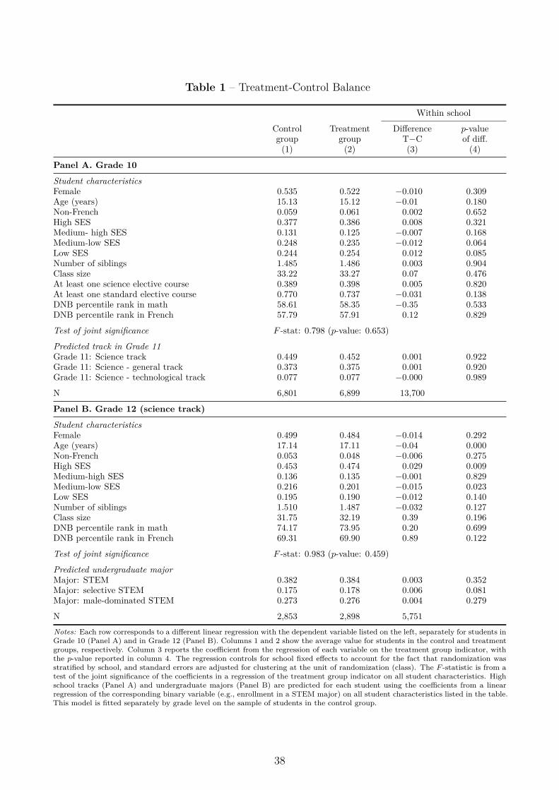
Table 1 – Treatment-Control Balance

Within school

Controlgroup

Treatmentgroup

DifferenceT−C

p-valueof diff.

(1) (2) (3) (4)

Panel A. Grade 10

Student characteristicsFemale 0.535 0.522 −0.010 0.309Age (years) 15.13 15.12 −0.01 0.180Non-French 0.059 0.061 0.002 0.652High SES 0.377 0.386 0.008 0.321Medium- high SES 0.131 0.125 −0.007 0.168Medium-low SES 0.248 0.235 −0.012 0.064Low SES 0.244 0.254 0.012 0.085Number of siblings 1.485 1.486 0.003 0.904Class size 33.22 33.27 0.07 0.476At least one science elective course 0.389 0.398 0.005 0.820At least one standard elective course 0.770 0.737 −0.031 0.138DNB percentile rank in math 58.61 58.35 −0.35 0.533DNB percentile rank in French 57.79 57.91 0.12 0.829

Test of joint significance F -stat: 0.798 (p-value: 0.653)

Predicted track in Grade 11Grade 11: Science track 0.449 0.452 0.001 0.922Grade 11: Science - general track 0.373 0.375 0.001 0.920Grade 11: Science - technological track 0.077 0.077 −0.000 0.989

N 6,801 6,899 13,700

Panel B. Grade 12 (science track)

Student characteristicsFemale 0.499 0.484 −0.014 0.292Age (years) 17.14 17.11 −0.04 0.000Non-French 0.053 0.048 −0.006 0.275High SES 0.453 0.474 0.029 0.009Medium-high SES 0.136 0.135 −0.001 0.829Medium-low SES 0.216 0.201 −0.015 0.023Low SES 0.195 0.190 −0.012 0.140Number of siblings 1.510 1.487 −0.032 0.127Class size 31.75 32.19 0.39 0.196DNB percentile rank in math 74.17 73.95 0.20 0.699DNB percentile rank in French 69.31 69.90 0.89 0.122

Test of joint significance F -stat: 0.983 (p-value: 0.459)

Predicted undergraduate majorMajor: STEM 0.382 0.384 0.003 0.352Major: selective STEM 0.175 0.178 0.006 0.081Major: male-dominated STEM 0.273 0.276 0.004 0.279

N 2,853 2,898 5,751Notes: Each row corresponds to a different linear regression with the dependent variable listed on the left, separately for students inGrade 10 (Panel A) and in Grade 12 (Panel B). Columns 1 and 2 show the average value for students in the control and treatmentgroups, respectively. Column 3 reports the coefficient from the regression of each variable on the treatment group indicator, withthe p-value reported in column 4. The regression controls for school fixed effects to account for the fact that randomization wasstratified by school, and standard errors are adjusted for clustering at the unit of randomization (class). The F -statistic is from atest of the joint significance of the coefficients in a regression of the treatment group indicator on all student characteristics. Highschool tracks (Panel A) and undergraduate majors (Panel B) are predicted for each student using the coefficients from a linearregression of the corresponding binary variable (e.g., enrollment in a STEM major) on all student characteristics listed in the table.This model is fitted separately by grade level on the sample of students in the control group.

38

Table 2 – Female Role Models: Summary Statistics

All rolemodels

Researchers(Ph.D./Postdoc)

Professionals(employed by

sponsoring firm)(1) (2) (3)

Age (N=51) 33.3 30.0 35.6(5.7) (3.1) (6.0)

Non-French 0.14 0.10 0.17

holds/prepares for a Ph.D. (N=55) 0.62 1.00 0.38

Graduated from a Grande École 0.39 0.33 0.43

Field: Math, Physics, Engineering 0.23 0.38 0.14

Field: Earth and Life Sciences 0.64 0.62 0.66

Field: Other 0.13 0.00 0.20

Has children (N=52) 0.42 0.19 0.58

Participated in the program the year before 0.25 0.19 0.29

Number of high schools visited 1.8 2.1 1.6(0.8) (0.9) (0.7)

Number of classroom interventions 5.2 5.9 4.7(2.3) (2.3) (2.1)

N 56 21 35Notes: The summary statistics are computed based on information obtained from the L’Oréal Foundation and from the post-intervention survey administered online to collect feedback about the classroom visits. Standard deviations are shown in parenthesesbelow the mean values. Where data are missing for some role models, the number of non-missing values N is indicated in parentheses.

39

Table 3 – Perceptions of Science-Related Careers

Girls Boys

Controlgroupmean

Treatmenteffect

(LATE)

p-value[q-value]

Controlgroupmean

Treatmenteffect

(LATE)

p-value[q-value]

(1) (2) (3) (4) (5) (6)

Panel A. Grade 10

Positive perceptions of science-related −0.020 0.245∗∗∗ 0.000 0.023 0.167∗∗∗ 0.000careers (index) (0.028) [0.001] (0.029) [0.001]

Science-related jobs require long years of study 0.839 −0.087∗∗∗ 0.000 0.849 −0.074∗∗∗ 0.000(0.010) [0.001] (0.010) [0.001]

Science-related jobs are monotonous 0.290 −0.032∗∗∗ 0.006 0.318 −0.006 0.633(0.012) [0.011] (0.013) [0.634]

Science-related jobs are solitary 0.325 −0.061∗∗∗ 0.000 0.303 −0.062∗∗∗ 0.000(0.012) [0.001] (0.011) [0.001]

Science-related jobs pay higher wages 0.637 0.008 0.535 0.668 0.015 0.237(0.014) [0.536] (0.013) [0.297]

Hard to maintain work-life balance 0.297 −0.026∗∗ 0.026 0.283 −0.029∗∗ 0.014(0.012) [0.033] (0.012) [0.023]

N 6,475 5,751

Panel B. Grade 12 (science track)

Positive perceptions of science-related −0.003 0.312∗∗∗ 0.000 0.003 0.155∗∗∗ 0.000careers (index) (0.034) [0.001] (0.033) [0.001]

Science-related jobs require long years of study 0.666 −0.110∗∗∗ 0.000 0.719 −0.091∗∗∗ 0.000(0.015) [0.001] (0.014) [0.001]

Science-related jobs are monotonous 0.169 −0.019 0.141 0.233 −0.026 0.114(0.013) [0.141] (0.016) [0.143]

Science-related jobs are solitary 0.228 −0.088∗∗∗ 0.000 0.206 −0.047∗∗∗ 0.000(0.012) [0.001] (0.013) [0.001]

Science-related jobs pay higher wages 0.531 0.059∗∗∗ 0.001 0.576 0.027∗ 0.093(0.018) [0.002] (0.016) [0.143]

Hard to maintain work-life balance 0.225 −0.049∗∗∗ 0.001 0.167 −0.012 0.260(0.015) [0.002] (0.011) [0.260]

N 2,600 2,636Notes: This table reports estimates of the treatment effects of classroom interventions on students’ perceptions of science-relatedcareers, separately by grade level and gender. The sample is restricted to students who completed the post-intervention questionnaire.Each row corresponds to a different linear regression performed separately by gender, with the dependent variable listed on the left.Columns 1 and 4 report the average value for students in the control group. Columns 2 and 5 report the local average treatmenteffect (LATE) estimates. They are obtained from a regression of the outcome of interest on a classroom visit indicator, usingtreatment assignment as an instrument for treatment receipt. The regression controls for school fixed effects to account for thefact that randomization was stratified by school. Standard errors (shown in parentheses) are adjusted for clustering at the unit ofrandomization (class). Columns 3 and 6 report the cluster-robust p-value of the estimated treatment effect and, in square brackets,the p-value (q-value) adjusted for multiple hypotheses testing, using the False Discovery Rate (FDR) control method. Specifically,we use the sharpened two-stage q-values introduced in Benjamini et al. (2006) and described in Anderson (2008). The q-valuesassociated with the synthetic index (highlighted in bold) are adjusted for multiple testing across the study’s nine main outcomes ofinterest, separately by grade level and gender (see Appendix D for details). The q-values for the individual components of the indexare adjusted for multiple testing across the index components, separately by grade level and gender. *** p < 0.01, ** p < 0.05,* p < 0.1.

40

Table 4 – Perceptions of Gender Roles in Science, Stated Preferences and Self-Concept

Girls Boys

Controlgroupmean

Treatmenteffect

(LATE)

p-value[q-value]

Controlgroupmean

Treatmenteffect

(LATE)

p-value[q-value]

(1) (2) (3) (4) (5) (6)

Panel A. Grade 10

Perceptions of gender roles in science

More men in science-related jobs 0.628 0.156∗∗∗ 0.000 0.629 0.168∗∗∗ 0.000(0.013) [0.001] (0.014) [0.001]

Equal gender aptitude for math (index) 0.115 0.109∗∗∗ 0.000 −0.134 0.148∗∗∗ 0.000(0.025) [0.001] (0.030) [0.001]

Women don’t really like science 0.157 0.059∗∗∗ 0.000 0.198 0.103∗∗∗ 0.000(0.011) [0.001] (0.013) [0.001]

W face discrimination in science-related jobs 0.603 0.127∗∗∗ 0.000 0.527 0.153∗∗∗ 0.000(0.013) [0.001] (0.014) [0.001]

Stated preferences and self-concept

Taste for science subjects (index) −0.169 −0.038 0.294 0.197 −0.019 0.533(0.036) [0.442] (0.031) [0.685]

Math self-concept (index) −0.198 −0.008 0.806 0.231 0.039 0.217(0.031) [0.807] (0.032) [0.326]

Science-related career aspirations (index) −0.103 0.012 0.695 0.120 0.007 0.801(0.030) [0.807] (0.029) [0.902]

N 6,475 5,751

Panel B. Grade 12 (science track)

Perceptions of gender roles in science

More men in science-related jobs 0.712 0.125∗∗∗ 0.000 0.717 0.149∗∗∗ 0.000(0.016) [0.001] (0.015) [0.001]

Equal gender aptitude for math (index) 0.158 0.095∗∗∗ 0.001 −0.161 0.132∗∗∗ 0.001(0.028) [0.002] (0.040) [0.002]

Women don’t really like science 0.074 0.044∗∗∗ 0.000 0.146 0.073∗∗∗ 0.000(0.009) [0.001] (0.015) [0.001]

W face discrimination in science-related jobs 0.624 0.095∗∗∗ 0.000 0.600 0.072∗∗∗ 0.000(0.020) [0.001] (0.018) [0.001]

Stated preferences and self-concept

Taste for science subjects (index) −0.002 0.016 0.632 0.002 −0.000 0.998(0.034) [0.633] (0.039) [0.999]

Math self-concept (index) −0.184 0.050 0.202 0.187 0.072∗∗ 0.041(0.039) [0.228] (0.035) [0.062]

Science-related career aspirations (index) −0.045 0.113∗∗∗ 0.002 0.046 0.050 0.131(0.037) [0.003] (0.033) [0.169]

N 2,600 2,636Notes: This table reports estimates of the treatment effects of classroom interventions on students’ perceptions of gender roles inscience, taste for science subjects, math self-concept, and science-related career aspirations, separately by grade level and gender.The sample is restricted to students who completed the post-intervention questionnaire. Each row corresponds to a different linearregression performed separately by gender, with the dependent variable listed on the left. Columns 1 and 4 report the averagevalue for students in the control group. Columns 2 and 5 report the local average treatment effect (LATE) estimates. They areobtained from a regression of the outcome of interest on a classroom visit indicator, using treatment assignment as an instrumentfor treatment receipt. The regression controls for school fixed effects to account for the fact that randomization was stratifiedby school. Standard errors (shown in parentheses) are adjusted for clustering at the unit of randomization (class). Columns 3and 6 report the cluster-robust p-value of the estimated treatment effect and, in square brackets, the p-value (q-value) adjusted formultiple hypotheses testing, using the False Discovery Rate (FDR) control method. Specifically, we use the sharpened two-stageq-values introduced in Benjamini et al. (2006) and described in Anderson (2008). The q-values are adjusted for multiple testingacross the study’s nine main outcomes of interest, separately by grade level and gender (see Appendix D for details). *** p < 0.01,** p < 0.05, * p < 0.1.

41

Table 5 – Enrollment Status the Following Year

Girls Boys

Controlgroupmean

Treatmenteffect

(LATE)

p-value[q-value]

Controlgroupmean

Treatmenteffect

(LATE)

p-value[q-value]

(1) (2) (3) (4) (5) (6)

Panel A. Grade 10

All STEM tracksGrade 11: Science track 0.355 −0.004 0.753 0.551 −0.002 0.910

(0.014) [0.807] (0.015) [0.910]

General vs. technological STEM trackGrade 11: Science - general track 0.328 0.001 0.942 0.416 0.007 0.613

(0.013) [0.942] (0.014) [0.614]

Grade 11: Science - technological track 0.026 −0.005 0.128 0.135 −0.009 0.300(0.003) [0.256] (0.008) [0.601]

Other tracks or repeaterGrade 11: Other tracks 0.545 0.006 0.642 0.324 0.018 0.191

(0.014) (0.014)

Repeater or dropout 0.101 −0.002 0.818 0.126 −0.016∗ 0.070(0.009) (0.009)

N 7,241 6,459

Panel B. Grade 12 (science track)

All undergraduate STEM majorsMajor: STEM 0.289 0.024∗ 0.080 0.470 0.003 0.886

(0.014) [0.103] (0.020) [0.998]

Selective vs. non-selective STEMMajor: selective STEM 0.110 0.035∗∗∗ 0.002 0.232 0.020 0.200

(0.011) [0.004] (0.016) [0.283]

Major: non-selective STEM 0.178 −0.011 0.322 0.239 −0.017 0.212(0.011) [0.322] (0.014) [0.283]

Male- vs. female-dominated STEMMajor: male-dominated STEM 0.166 0.038∗∗∗ 0.002 0.379 0.017 0.387(math, physics, computer science) (0.012) [0.004] (0.019) [0.388]

Major: female-dominated STEM 0.123 −0.015 0.158 0.091 −0.014 0.119(earth and life sciences) (0.010) [0.211] (0.009) [0.283]

Other tracks or dropoutOther non-STEM programs 0.507 −0.032∗∗ 0.045 0.293 −0.005 0.717

(0.016) (0.014)

Not enrolled in a post-graduate curriculum 0.206 0.008 0.581 0.237 0.004 0.814(0.015) (0.016)

N 2,827 2,924Notes: This table reports estimates of the treatment effects of classroom interventions on students’ enrollment outcomes in theacademic year following the classroom interventions, i.e. 2016/17, separately by grade level and gender. The enrollment outcomesare measured using student-level administrative data. Each row corresponds to a different linear regression performed separately bygender, with the dependent variable listed on the left. Columns 1 and 4 report the average value for students in the control group.Columns 2 and 5 report the local average treatment effect (LATE) estimates. They are obtained from a regression of the outcome ofinterest on a classroom visit indicator, using treatment assignment as an instrument for treatment receipt. The regression controlsfor school fixed effects to account for the fact that randomization was stratified by school. Standard errors (shown in parentheses)are adjusted for clustering at the unit of randomization (class). Columns 3 and 6 report the cluster-robust p-value of the estimatedtreatment effect and, in square brackets, the p-value (q-value) adjusted for multiple hypotheses testing, using the False DiscoveryRate (FDR) control method. Specifically, we use the sharpened two-stage q-values introduced in Benjamini et al. (2006) anddescribed in Anderson (2008). The q-values associated with the treatment effect estimates on “Grade 11: Science track” (Panel A)and “Major: STEM” (Panel B) are adjusted for multiple testing across the study’s nine main outcomes of interest, separately bygrade level and gender (see Appendix D for details). The q-values associated with the treatment effect estimates for the differentSTEM tracks (Panel A) or the different STEM majors (Panel B) are adjusted for multiple testing across these different STEMtracks or majors, separately by grade level and gender. *** p < 0.01, ** p < 0.05, * p < 0.1.

42

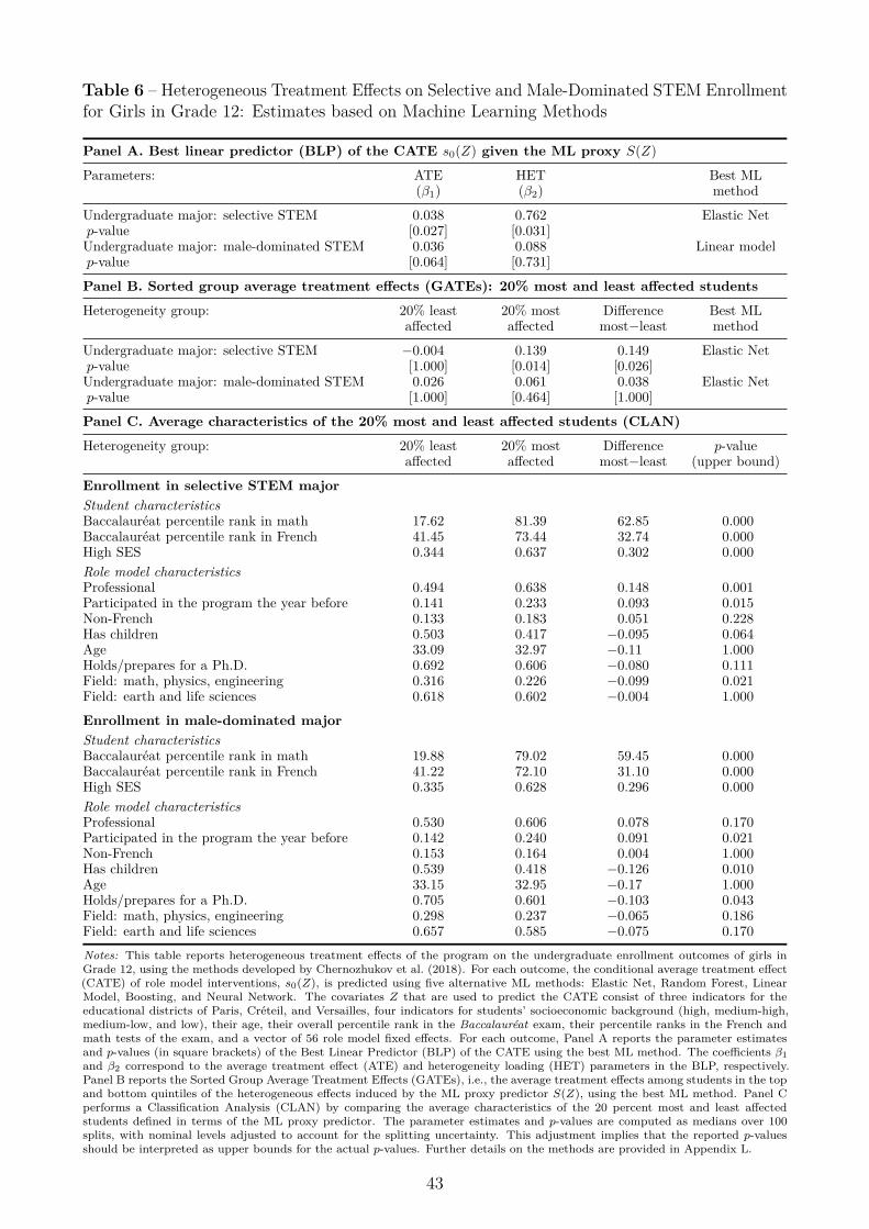
Table 6 – Heterogeneous Treatment Effects on Selective and Male-Dominated STEM Enrollmentfor Girls in Grade 12: Estimates based on Machine Learning Methods

Panel A. Best linear predictor (BLP) of the CATE s0(Z) given the ML proxy S(Z)

Parameters: ATE HET Best ML(β1) (β2) method

Undergraduate major: selective STEM 0.038 0.762 Elastic Netp-value [0.027] [0.031]Undergraduate major: male-dominated STEM 0.036 0.088 Linear modelp-value [0.064] [0.731]

Panel B. Sorted group average treatment effects (GATEs): 20% most and least affected students

Heterogeneity group: 20% least 20% most Difference Best MLaffected affected most−least method

Undergraduate major: selective STEM −0.004 0.139 0.149 Elastic Netp-value [1.000] [0.014] [0.026]Undergraduate major: male-dominated STEM 0.026 0.061 0.038 Elastic Netp-value [1.000] [0.464] [1.000]

Panel C. Average characteristics of the 20% most and least affected students (CLAN)

Heterogeneity group: 20% least 20% most Difference p-valueaffected affected most−least (upper bound)

Enrollment in selective STEM majorStudent characteristicsBaccalauréat percentile rank in math 17.62 81.39 62.85 0.000Baccalauréat percentile rank in French 41.45 73.44 32.74 0.000High SES 0.344 0.637 0.302 0.000Role model characteristicsProfessional 0.494 0.638 0.148 0.001Participated in the program the year before 0.141 0.233 0.093 0.015Non-French 0.133 0.183 0.051 0.228Has children 0.503 0.417 −0.095 0.064Age 33.09 32.97 −0.11 1.000Holds/prepares for a Ph.D. 0.692 0.606 −0.080 0.111Field: math, physics, engineering 0.316 0.226 −0.099 0.021Field: earth and life sciences 0.618 0.602 −0.004 1.000

Enrollment in male-dominated majorStudent characteristicsBaccalauréat percentile rank in math 19.88 79.02 59.45 0.000Baccalauréat percentile rank in French 41.22 72.10 31.10 0.000High SES 0.335 0.628 0.296 0.000Role model characteristicsProfessional 0.530 0.606 0.078 0.170Participated in the program the year before 0.142 0.240 0.091 0.021Non-French 0.153 0.164 0.004 1.000Has children 0.539 0.418 −0.126 0.010Age 33.15 32.95 −0.17 1.000Holds/prepares for a Ph.D. 0.705 0.601 −0.103 0.043Field: math, physics, engineering 0.298 0.237 −0.065 0.186Field: earth and life sciences 0.657 0.585 −0.075 0.170Notes: This table reports heterogeneous treatment effects of the program on the undergraduate enrollment outcomes of girls inGrade 12, using the methods developed by Chernozhukov et al. (2018). For each outcome, the conditional average treatment effect(CATE) of role model interventions, s0(Z), is predicted using five alternative ML methods: Elastic Net, Random Forest, LinearModel, Boosting, and Neural Network. The covariates Z that are used to predict the CATE consist of three indicators for theeducational districts of Paris, Créteil, and Versailles, four indicators for students’ socioeconomic background (high, medium-high,medium-low, and low), their age, their overall percentile rank in the Baccalauréat exam, their percentile ranks in the French andmath tests of the exam, and a vector of 56 role model fixed effects. For each outcome, Panel A reports the parameter estimatesand p-values (in square brackets) of the Best Linear Predictor (BLP) of the CATE using the best ML method. The coefficients β1and β2 correspond to the average treatment effect (ATE) and heterogeneity loading (HET) parameters in the BLP, respectively.Panel B reports the Sorted Group Average Treatment Effects (GATEs), i.e., the average treatment effects among students in the topand bottom quintiles of the heterogeneous effects induced by the ML proxy predictor S(Z), using the best ML method. Panel Cperforms a Classification Analysis (CLAN) by comparing the average characteristics of the 20 percent most and least affectedstudents defined in terms of the ML proxy predictor. The parameter estimates and p-values are computed as medians over 100splits, with nominal levels adjusted to account for the splitting uncertainty. This adjustment implies that the reported p-valuesshould be interpreted as upper bounds for the actual p-values. Further details on the methods are provided in Appendix L.

43

Table 7 – Heterogeneous Treatment Effects on Student Perceptions: Average Characteristics ofthe Most and Least Affected Girls in Grade 12

20% least 20% most Difference p-valueaffected affected most−least (upper bound)

(1) (2) (3) (4)

Positive perceptions of science-related careers (index)Mean Baccalauréat percentile rank in math 26.62 73.29 46.85 0.000Class visited by professional 0.483 0.675 0.192 0.000

More men in science-related jobsMean Baccalauréat percentile rank in math 74.87 25.00 −51.03 0.000Class visited by professional 0.614 0.511 −0.112 0.031

Equal gender aptitude for math (index)Mean Baccalauréat percentile rank in math 42.77 50.58 7.89 0.003Class visited by professional 0.622 0.563 −0.058 0.403

Women don’t really like scienceMean Baccalauréat percentile rank in math 44.47 50.57 5.07 0.090Class visited by professional 0.592 0.540 −0.035 0.908

Women face discrimination in science-related jobsMean Baccalauréat percentile rank in math 52.15 42.79 −8.81 0.001Class visited by professional 0.568 0.570 0.011 1.000

Taste for science subjects (index)Mean Baccalauréat percentile rank in math 41.36 54.71 13.63 0.000Class visited by professional 0.436 0.678 0.227 0.000

Math self-concept (index)Mean Baccalauréat percentile rank in math 52.22 42.10 −10.65 0.000Class visited by professional 0.512 0.582 0.071 0.240

Science-related career aspirations (index)Mean Baccalauréat percentile rank in math 44.70 47.78 2.36 0.712Class visited by professional 0.375 0.762 0.389 0.000

Notes: This table reports the average characteristics of Grade 12 girls in the top and bottom quintile of predicted treatmenteffects on student perceptions, using the methods developed by Chernozhukov et al. (2018). For each outcome, the conditionalaverage treatment effect (CATE) of role model interventions, s0(Z), is predicted using five alternative ML methods: Elastic Net,Random Forest, Linear Model, Boosting, and Neural Network. The covariates Z that are used to predict the CATE consist of threeindicators for the educational districts of Paris, Créteil, and Versailles, four indicators for students’ socioeconomic background (high,medium-high, medium-low, and low), their age, their overall percentile rank in the Baccalauréat exam, their percentile ranks in theFrench and math tests of the exam, and a vector of 56 role model fixed effects. For each outcome, the table compares the averagecharacteristics of the students in the top and bottom quintile of treatment effects, as predicted by the best ML proxy predictorbased on the Group average treatment effects (GATEs) targeting of the CATE. The characteristics reported in this table are thestudents’ average percentile rank in math in the Baccalauréat exams and the share exposed to a role model with a professionalrather a research background. The parameter estimates and p-values are computed as medians over 100 splits, with nominal levelsadjusted to account for the splitting uncertainty. This adjustment implies that the reported p-values should be interpreted as upperbounds for the actual p-values. The average treatment effects among the 20 percent most and least affected students can be foundin Panel B of Appendix Table L1. Further details on the methods are provided in Appendix L.

44

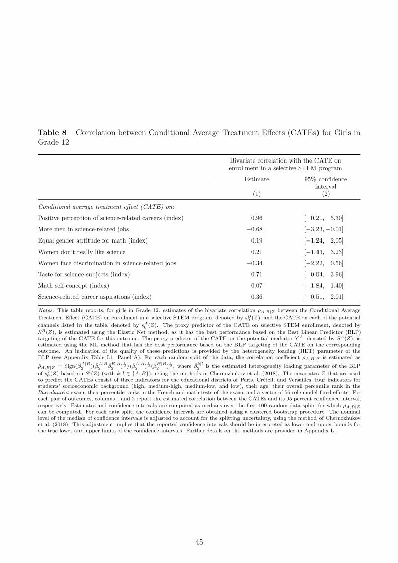
Table 8 – Correlation between Conditional Average Treatment Effects (CATEs) for Girls inGrade 12

Bivariate correlation with the CATE onenrollment in a selective STEM program

Estimate 95% confidenceinterval

(1) (2)

Conditional average treatment effect (CATE) on:

Positive perception of science-related careers (index) 0.96 [ 0.21, 5.30]

More men in science-related jobs −0.68 [−3.23,−0.01]

Equal gender aptitude for math (index) 0.19 [−1.24, 2.05]

Women don’t really like science 0.21 [−1.43, 3.23]

Women face discrimination in science-related jobs −0.34 [−2.22, 0.56]

Taste for science subjects (index) 0.71 [ 0.04, 3.96]

Math self-concept (index) −0.07 [−1.84, 1.40]

Science-related career aspirations (index) 0.36 [−0.51, 2.01]

Notes: This table reports, for girls in Grade 12, estimates of the bivariate correlation ρA,B|Z between the Conditional AverageTreatment Effect (CATE) on enrollment in a selective STEM program, denoted by sB

0 (Z), and the CATE on each of the potentialchannels listed in the table, denoted by sA

0 (Z). The proxy predictor of the CATE on selective STEM enrollment, denoted bySB(Z), is estimated using the Elastic Net method, as it has the best performance based on the Best Linear Predictor (BLP)targeting of the CATE for this outcome. The proxy predictor of the CATE on the potential mediator Y A, denoted by SA(Z), isestimated using the ML method that has the best performance based on the BLP targeting of the CATE on the correspondingoutcome. An indication of the quality of these predictions is provided by the heterogeneity loading (HET) parameter of theBLP (see Appendix Table L1, Panel A). For each random split of the data, the correlation coefficient ρA,B|Z is estimated asρA,B|Z = Sign(βA|B

2 )(βA|B2 β

B|A2 )

12 /(βA|A

2 )12 (βB|B

2 )12 , where βk|l

2 is the estimated heterogeneity loading parameter of the BLPof sk

0(Z) based on Sl(Z) (with k, l ∈ {A,B}), using the methods in Chernozhukov et al. (2018). The covariates Z that are usedto predict the CATEs consist of three indicators for the educational districts of Paris, Créteil, and Versailles, four indicators forstudents’ socioeconomic background (high, medium-high, medium-low, and low), their age, their overall percentile rank in theBaccalauréat exam, their percentile ranks in the French and math tests of the exam, and a vector of 56 role model fixed effects. Foreach pair of outcomes, columns 1 and 2 report the estimated correlation between the CATEs and its 95 percent confidence interval,respectively. Estimates and confidence intervals are computed as medians over the first 100 random data splits for which ρA,B|Zcan be computed. For each data split, the confidence intervals are obtained using a clustered bootstrap procedure. The nominallevel of the median of confidence intervals is adjusted to account for the splitting uncertainty, using the method of Chernozhukovet al. (2018). This adjustment implies that the reported confidence intervals should be interpreted as lower and upper bounds forthe true lower and upper limits of the confidence intervals. Further details on the methods are provided in Appendix L.

45

(For Online Publication)

Appendix to

Do female Role Models Reduce the Gender Gap inScience? Evidence from French High Schools

Thomas BredaJulien GrenetMarion Monnet

Clémentine Van Effenterre

List of Appendices

A Gender Pay Gap Among College Graduates in France A-2

B Program Details A-8

C Student-Level Administrative Data A-10

D Construction of Synthetic Indices and Multiple Hypotheses Testing A-12

E Summary Statistics and Balancing Tests A-14

F Effects of Role Model Interventions: Additional Results A-21

G Robustness Checks A-28

H Randomization Inference A-30

I Information, Persistence, Timing: Additional Results A-32

J Spillover Effects A-37

K Heterogeneous Treatment Effects: Subgroup Analysis A-47

L Heterogeneous Treatment Effects: Machine Learning Methods A-50

Appendix References A-60

A-1

A Gender Pay Gap Among College Graduates in FranceThis appendix provides descriptive evidence on the entry-level gender pay gap among Frenchcollege graduates holding a master’s degree and analyzes the contribution of gender segregationin college majors to this gap. The objective of this analysis is to better understand whether theeffects of the role model interventions on female students’ choice of study can be expected toreduce the gender pay gap. Section A.1 describes the data sources, while Section A.2 discussesthe empirical results.

A.1 DataUnfortunately, we cannot rely exclusively on administrative data to provide empirical evidenceon the gender pay gap by field of study in France, as it is currently not possible to linkadministrative data on students enrolled in higher education with administrative data on wagesand income tax returns. Instead, our analysis is based on the combination of aggregate statisticson student enrollment by college major and gender with survey information on the startingwages of recent cohorts of college graduates.

Data sources. In France, gender segregation and gender pay gaps by college major canbe analyzed for the population of college graduates who obtained their master’s degree (orequivalent) in 2015 or 2016. For this purpose, we combine several administrative and surveydata sources.

SISE Résultats 2015. This individual-level administrative dataset covers all students enrolledin public universities during the academic year 2015/16 and provides detailed information oneach student’s degree program and field of study.

Enquête Professionnelle des Diplômés de Master 2015 (EPDM). This survey was conductedin December 2017 by the Ministry of Higher Education to collect information on the transitionof master’s graduates to the labor market. The survey was targeted at students who obtainedtheir master’s degree in 2015 and who entered the labor market within one year after graduation,with an overall response rate of 70 percent. As part of this survey, master’s graduates wereasked to report their annual earnings 18 months after graduation. Our analyses are based onthe survey’s public use files, which provide aggregate statistics by gender and college major.A.1

Enquête sur l’Insertion des Diplômés des Grandes Écoles 2018 (EIDGE). This survey wasconducted in 2018 by the Conférence des Grandes Écoles (CGE), a not-for-profit associationrepresenting French elite graduate schools. The Grandes Écoles, which award a diplomaequivalent to a master’s degree, recruit their students through highly competitive national examstaking place at the end of two-year undergraduate selective STEM and non-STEM preparatorycourses (Classes Préparatoires aux Grandes Écoles or CPGE). The survey was targeted atstudents who graduated between 2015 and 2017 from one of the 184 Grandes Écoles that weremembers of the CGE in 2018, with an overall response rate of 48 percent. Our analyses arebased on the aggregate statistics published by the CGE separately by gender and by type ofGrande École (i.e., engineering schools, business schools, and other schools).A.2 We only considerstudents who graduated from a Grande École in 2016, since annual earnings 24 months aftergraduation are only available for this cohort.

A.1https://data.enseignementsup-recherche.gouv.fr/explore/dataset/fr-esr-insertion_professionnelle-master_donnees_nationales/information/ (accessed on August 2, 2019).

A.2https://www.cge.asso.fr/themencode-pdf-viewer/?file=https://www.cge.asso.fr/wp-content/uploads/2018/06/2018-06-19-Rapport-2018.pdf (accessed on August 2, 2019).

A-2

Grouping of college majors. The above data sources can be combined to compute thenumber of female and male master’s students who graduated from university in 2015 or from aGrande École in 2016, separately by college major.

The Ministry of Higher Education’s official classification comprises 54 college majors. Forthe purpose of our analysis, we group these college majors into the following broad categories:

• Non-STEM majors (35 in total): this category includes master’s degree programs in law,economics, management, humanities, psychology, social sciences, medicine, pharmacy,sports studies as well as degrees from non-STEM Grande Écoles (e.g., business schools,schools of journalism, schools of architecture).

• STEM majors (19 in total): this category includes master’s degree programs in STEMfields as well as degrees from engineering schools (Grande Écoles d’ingénieurs).

• Among STEM majors, we distinguish between engineering schools (all of which are selectiveand are classified as a single major) and non-selective STEM master’s degrees at university(18 in total).

• Among non-selective STEM majors, we further distinguish between male-dominatedmajors (16 in total) and female-dominated majors (2 in total: chemistry and earth andlife sciences), based on whether the share of female students among master’s graduates inthe corresponding field of study is below or above 50 percent. This distinction does notapply to selective STEM majors, since almost all engineering schools are male-dominated.

Earnings information. The EPDM and EIDGE surveys provide information on graduates’average median gross salary (salaire brut annuel médian) separately by gender and college major.Starting wages are measured 18 months after graduation for master’s graduates and 24 monthsafter graduation for Grandes Écoles graduates. Note that since we do not have access to theindividual-level survey data, median earnings by broad categories of college majors can onlybe approximated as the average of the median earnings in each of the majors that form thesebroad categories.

A.2 College Majors and the Gender Pay GapCombining the above data sources, we provide descriptive evidence on the median startingwages of female and male graduates across the broad categories of college majors. We thenanalyze the contribution of gender segregation in college majors to the overall entry-level genderpay gap.

Gender composition of STEM and non-STEM majors. The first three columns ofTable A1 show the distribution of master’s-level graduates across the broad categories of collegemajors defined above, along with the share of female graduates in each category. The summarystatistics indicate that while female students represent 52 percent of master’s level graduates,they are strongly underrepresented in STEM majors (34 percent). Female underrepresentationis more pronounced in selective (male-dominated) STEM majors (female share: 30 percent)than in non-selective STEM majors (female share: 40 percent). Among non-selective STEMmajors, female students represent only 29 percent of graduates in male-dominated fields suchas mathematics, physics, or computer science, compared to 60 percent of graduates in female-dominated fields such as chemistry and earth and life sciences.

Starting wages of STEM and non-STEM graduates. The comparison of starting wagesby broad college major category confirms that female graduates tend to be overrepresentedin lower-paying majors (see columns 3–5 of Table A1). Female graduates holding a STEM

A-3

degree have a median starting wage of 29,984 euros, which is 7.4 percent higher than the medianstarting wage of female graduates holding a non-STEM degree (27,913 euros). Strikingly, thewage premium for female graduates in STEM appears to be almost entirely driven by selective(male-dominated) STEM degrees (16.4 percent). By contrast, the wage premium attachedto non-selective STEM degrees is close to zero (−0.5 percent). The low apparent return tonon-selective STEM degrees masks substantially different returns between male-dominated andfemale-dominated majors: while the wage premium attached to male-dominated non-selectiveSTEM majors is of 4.2 percent for female graduates compared to non-STEM majors, a wagepenalty of 4.7 percent is attached to female-dominated non-selective STEM majors.

Female underrepresentation in STEM: contribution to the gender pay gap. Thelast three columns of Table A1 indicate that across all categories of programs, male graduatesearn a median annual starting wage of 32,122 euros, compared to 28,411 euros for femalegraduates. This amounts to an overall gender pay gap of 3,711 euros per year, or 11.6 percentof male pay.

Although the overrepresentation of female graduates in lower-paying non-STEM and female-dominated STEM majors is a likely contributor to the overall gender pay gap, it is clearly notthe sole cause, as gender differences in median earnings are observed within each broad categoryof college majors. Interestingly, however, the gender wage gap is lower in each category of STEMmajors than in non-STEM majors. This finding is consistent with similar evidence for the U.S.(Beede et al., 2011).

To shed light on the contribution of gender segregation in fields of study to the overallentry-level gender pay gap, we adopt a method similar to that used by McDonald and Thornton(2007) in estimating what the overall female-male starting wage gap would be if female graduateshad the same distribution of college majors as male graduates.

Since our interest is in measuring the specific contribution of the different dimensions offemale underrepresentation in STEM majors (STEM vs. non-STEM, selective vs. non-selectiveSTEM, male-dominated vs. female-dominated non-selective STEM), we construct counterfactualwage gaps by considering increasingly disaggregated groups of majors.

We start by estimating the counterfactual wage gap if female graduates had the samedistribution of STEM vs. non-STEM majors as male graduates, while keeping fixed females’marginal distribution of majors within each of these two broad categories. Put differently,we apply female median earnings in STEM vs. non-STEM degrees to the male distributionof graduates in both categories of majors to recalculate the overall gender pay gap. Thiscounterfactual wage gap, which we denote by ∆w, is constructed as follows:

∆w = 1− (wfsNms + wfnsN

mns)

(wms Nms + wmnsN

mns)

,

where wgk and N gk denote the median earnings and the number of graduates of gender g (m:

males; f : females) in college major category k (s: STEM; ns: non-STEM), respectively. Thecontribution of female underrepresentation in STEM programs to the gender pay gap is thenmeasured as ∆w− ∆w, where ∆w denotes the observed overall pay gap between male and femalegraduates.

To measure the contribution of gender segregation between selective and non-selectiveSTEM majors, we construct a second counterfactual wage gap in a similar manner, exceptthat college majors are now grouped into three categories: non-STEM, selective STEM, andnon-selective STEM. To measure the contribution of gender segregation between male-dominatedand female-dominated STEM majors, we repeat this exercise after grouping college majorsinto four categories: non-STEM, selective STEM, non-selective male-dominated STEM, and

A-4

non-selective female-dominated STEM. The contribution of gender segregation between majorswithin both male- and female-dominated non-selective STEM is measured by ungrouping allSTEM majors. Finally, we ungroup all non-STEM majors to evaluate the contribution of gendersegregation between non-STEM majors. The corresponding counterfactual measures what theoverall gender gap would be if women had the same distribution as men across all 54 STEMand non-STEM college majors.

Results. The results of this decomposition exercise are shown in Table A2 along with theobserved gender pay gap. The contributions of gender segregation between the different categoriesof college majors to the gender pay gap are reported in column 1 and are expressed as percentagesof the total in column 2. We find that the gender imbalances across all college majors “explain”40 percent of the gender pay gap among college graduates. Two-thirds of this explained part(26.5 percent of the total wage gap) can be attributed to the unequal representation of femaleand male graduates in STEM vs. non-STEM majors, on the one hand, and between the differentmajors within STEM, on the other hand. The remain third of the explained part of thegap (13.4 percent of the total) is due to gender segregation between non-STEM majors, thelowest-paying majors (humanities) being typically more female-dominated (77 percent) than thehighest-paying ones (law and economics, where the female share is 59 percent).

The 26.5 percent STEM-related gender pay gap can be decomposed as follows. Increasingthe share of female graduates holding a STEM degree to that of males without changing females’marginal distribution of STEM majors is associated with a 14.0 percent reduction in the genderpay gap. In line with the evidence from Table A1, further reassigning female graduates fromnon-selective STEM majors to (male-dominated) selective STEM majors in order to matchthe relative shares of selective and non-selective STEM majors among male graduates wouldreduce the gender gap by an additional 6.5 percent from the baseline. Finally, reassigning femalegraduates from non-selective female-dominated STEM majors to non-selective male-dominatedSTEM majors would trigger an extra 4.3 percent reduction in the gender pay gap, while furtherreassigning female students between majors within male- and female-dominated programs wouldresult in an extra 1.8 percent reduction from the baseline.

Altogether, these findings suggest that the underrepresentation of female students in STEMmajors accounts for approximately 25 percent of the entry-level gender pay gap among collegegraduates in France. Almost half of this STEM-related gender pay gap can be attributed tothe fact that within STEM majors, female graduates are relatively less likely than males to beenrolled in those with the largest wage premium, i.e., the selective and male-dominated STEMmajors.

A-5

Table A1 – Starting Wage Among College Graduates Holding a Master’s Degree or Equivalent, Classes of 2015/16

Graduates: classes of 2015/16 Wage 18/24 months after graduation (survey)

Female graduates Male graduates

Number ofgraduates

% oftotal

Femaleshare(%)

Medianwage(euros)

RelativeMedianwage

(non-STEMmajors: 100)

Medianwage(euros)

RelativeMedianwage

(non-STEMmajors: 100)

Genderpay gap(%)

(1) (2) (3) (4) (5) (6) (7) (8)

All majors (54) 166,600 100.0 51.5 28,411 - 32,122 - 11.6

Non-STEM majors (35) 106,997 64.2 61.1 27,913 100.0 31,302 100.0 10.8

STEM majors (19) 59,603 35.8 34.3 29,984 107.4 32,972 105.3 9.1

of which:

Selective (male-dominated) STEM 31,463 18.9 29.7 32,500 116.4 34,800 111.2 6.6majors (Engineering schools)

Non-Selective STEM 28,140 16.9 39.6 27,767 99.5 30,530 97.5 9.1majors (18)

of which:

Male-dominated majors (16) 18,874 11.3 29.4 29,077 104.2 31,371 100.2 7.3

Female-dominated majors (2) 9,266 5.6 60.3 26,596 95.3 27,581 88.1 3.6Notes: This table reports summary statistics on gender segregation and gender pay gaps for the population of college graduates who obtained their master’s degree (or equivalent) in 2015 or 2016.The 54 college majors are grouped into two broad categories: non-STEM majors (master’s degrees in economics, management, humanities, psychology, social sciences, sports studies, medicine,pharmacy, and non-STEM Grandes Écoles such as business schools or schools of journalism) and STEM majors (master’s degrees in STEM fields and degrees from engineering schools); STEMmajors are further broken down between selective (engineering schools) and non-selective majors (master’s degree at university); among non-selective majors, we distinguish between male-dominatedand female-dominated majors, based on whether the share of female graduates in the corresponding field of study is below or above 50 percent. Column 1 shows the number of graduates per broadcategory of college majors using the administrative dataset SISE 2015/16 (for university graduates who obtained their master’s degree in 2016) and the EIDGE survey (for students who graduatedfrom Grandes Écoles in 2016). Median gross annual wages (columns 4 and 6) are computed from aggregate statistics by gender and college major from the EPDM and EIDGE surveys. Entry-levelwages are measured 18 months after graduation for master’s graduates and 24 months after graduation for Grandes Écoles graduates. Median wages by broad categories of college majors areapproximated as the average of the median wages in each of the majors that form these broad categories.Sources: Columns 1–3: SISE 2015/16 and Enquête sur l’Insertion des Diplômés des Grandes Écoles 2018 (EIDGE); columns 4–8: Enquête Professionnelle des Diplômés de Master 2015 (EPDM) andEIDGE.

A-6

Table A2 – Contribution of Gender Segregation in College Majors to the Entry-Level GenderWage Gap Among College Graduates, Classes of 2015/16

Genderpay gap

(relative tomale pay)

Shareof thegender

wage gap(1) (2)

Total wage gap 0.116 100.0%

Contribution of gender segregation in college majors to the wage gap:

Explained by unequal gender distribution between majors 0.046 40.0%

of which:

between STEM/non-STEM majors and between majors within STEM 0.031 26.5%

of which:

between STEM and non-STEM majors 0.016 14.0%between selective and non-selective STEM majors 0.007 6.5%between male- and female-dominated non-selective STEM majors 0.005 4.3%between majors within male- and female-dominated non-selective STEM 0.002 1.8%

between majors within non-STEM 0.016 13.4%

Unexplained by unequal gender distribution between majors 0.069 60.0%Notes: This table provides a decomposition of the total entry-level wage gap between male and female college graduates whoobtained their master’s degree or equivalent in 2015 (university graduates) or in 2016 (Grandes Écoles graduates). Entry-levelwages are measured as median annual gross wages by gender and college major, 18 months after graduation for master’s graduates,and 24 months after graduation for Grandes Écoles graduates. To measure the contribution of the unequal gender representationacross college majors, counterfactual wage gaps are constructed using increasingly disaggregated groups of college majors. Thecontribution of gender segregation between STEM and non-STEM majors is measured as the observed gender wage gap minus thecounterfactual wage gap that would be observed if female graduates had the same distribution of STEM and non-STEM majorsas male graduates, while keeping fixed females’ marginal distribution of majors within each of these two broad categories. Thecontribution of gender segregation between selective and non-selective STEM majors is estimated in a similar manner, except thatthe counterfactual gender wage gap is estimated by reassigning female graduates from non-selective STEM majors to selective STEMmajors to match the relative shares of selective and non-selective STEM majors among male graduates. The other components ofthe gender wage gap are measured by sequentially ungrouping college majors to compute counterfactual gender wage gaps. Thecontributions of gender segregation between the different categories of college majors to the gender wage gap are shown in column 1and are expressed as percentages of the total in column 2.Sources: See notes of Table A1.

A-7

B Program Details

(a) First Video: “Jobs in Science: Beliefs or Reality?”

(b) Second Video: “Are we All Equal in Science?”

Figure B1 – Screenshots of the Two Videos Shown During the Role Model Interventions

A-8

Figure B2 – Screenshots of the Slides Provided to the Role Models to Describe their ownExperience

!(!(!(!(

!(!(!(

!(

!(

!(!(!(

!(

!(

!(

!(

!(

!(

!(

!(

!(

!(

!(

!(

!(

!(

!(

!(

!(

!(

!(

!(

!(

!(

!(

!(

!(

!(

!(

!(

!(

!(

!(

!(

!(!(

!(

!(

!(

!(

!(

!(

!(

!(

!(

!(

!(

!(!(

!(

!(

!(

!(

!(

!(!(

!(

!(!(!(

!(

!(

!(

!(!(

!(!(

!(

!( !(

!(

!(

!(

!(

!(

!(

!(

!(

!(!(!(

!(

!(

!(

!(

!(

!(

!(

Créteil

Versailles

Paris

0 10 205 km

Figure B3 – Participating High SchoolsNotes: The thick lines represent the boundaries of the three education districts (académies) of the Paris region (Paris, Créteil andVersailles). The solid circles show the location of the 98 high schools that participated in the program evaluation.

A-9

C Student-Level Administrative DataThis appendix describes the administrative data that we use to complement the informationfrom the student survey (Section C.1) and provides details about the classification of STEMundergraduate programs (Section C.2).

C.1 Data SourcesFor the purpose of the empirical analysis, we matched the data from our post-interventionstudent survey with three administrative datasets. These data were linked using an encryptedversion of the French national student identifier (Identifiant National Élève).

High school enrollment data. Students’ socio-demographic characteristics and enrollmentstatus are obtained from the Bases Élèves Académiques (BEA) for academic years 2012/13to 2016/17. These comprehensive administrative registers, which were provided by the threeeducation districts of the Paris region (Paris, Créteil, and Versailles), cover the universe ofstudents enrolled in the public and private high schools operating in the three districts. Theyalso cover students enrolled in selective undergraduate programs, i.e., Classes préparatoires auxGrandes Écoles (CPGE) and Sections de technicien supérieur (STS), as these programs arelocated in high schools. The BEA data provide basic information on students’ demographics(gender, date and country of birth, number of siblings), their parents’ two-digit occupation, anddetailed information on their enrollment status (school and class attended, elective courses taken).Students’ socioeconomic status (SES) is measured using the French Ministry of Education’sofficial classification, which uses the occupation of the child’s legal guardian to define fourgroups of SES: high (company managers, executives, liberal professions, engineers, intellectualoccupations, arts professions), medium-high (technicians and associate professionals), medium-low (farmers, craft and trades workers, service and sales workers), and low (manual workers andpersons without employment).

University enrollment data. To track Grade 12 (science track) students’ enrollment out-comes in non-selective undergraduate programs (Licence), we use a separate administrativedata source, the Système d’Information sur le Suivi de l’Étudiant (SISE), which is managed bythe Statistical Office of the French Ministry of Higher Education (Sous-Direction des Systèmesd’Information et des Études Statistiques, MESRI-SIES). This dataset, which covers the academicyears 2012/13 to 2016/17, records all students enrolled in the French higher education systemoutside of CPGE and STS, except for the small fraction of students enrolled in undergraduateprograms leading to paramedical and social care qualifications.

Data on student performance. The third dataset, the Organisation des Concours etExamens Académiques et Nationaux (OCEAN), contains students’ individual exam results forthe Diplôme national du brevet (DNB), which middle school students take at the end Grade 9,and for the Baccalauréat, which high school students take at the end of Grade 12. Access to thisdataset, which covers the exams years 2010 to 2016, was provided by the Statistical Office of theFrench Ministry of Education (Direction de l’Évaluation, de la Prospective et de la Performance,MENJ-DEPP).

C.2 Classification of STEM Undergraduate ProgramsThe enrollment status of Grade 12 (science track) students in the year following the intervention,i.e., 2016/17, is measured by combing the information from the BEA and SISE datasets. For the

A-10

purpose of our analysis, we use two alternative classifications of STEM undergraduate programs,based on whether they are (i) selective or non-selective, and (ii) male- or female-dominated.

Selective vs. non-selective STEM programs.

• Selective STEM : This category includes all CPGE programs with a specialization inSTEM, i.e., mathematics, physics and engineering science (MPSI), physics, chemistry andengineering science (PCSI), biology, chemistry, physics and earth sciences (BCPST), andphysics, technology, and engineering science (PTSI). It also includes a small number ofselective programs in engineering schools that recruit their students directly after highschool graduation, as well as selective technical/vocational undergraduate programs (STS)that specialize in STEM fields.

• Non-selective STEM : This category includes non-selective university bachelor’s degreeprograms (Licence) that specialize in STEM fields: math, physics, chemistry, earth andlife sciences, and computer science. Undergraduate programs in medicine and pharmacyare not included in this category.

Male- vs. female-dominated STEM programs.

• Male-dominated STEM : We consider as male-dominated STEM programs those in whichthe share of female students is less than 50 percent. This category includes the selectiveprograms (CPGE and STS) and non-selective programs (Licence) that specialize inmathematics, physics, chemistry, computer science, and engineering.

• Female-dominated STEM : This category includes both selective (CPGE and STS) andnon-selective programs (Licence) that specialize in earth and life sciences.

If a student is enrolled in multiple higher education programs, we only consider the mostselective among these programs, with CPGE taking precedence over STS, and STS takingprecedence over university undergraduate degree programs.

A-11

D Construction of Synthetic Indices and Multiple Hy-potheses Testing

This appendix discusses the construction of the synthetic indices that we use to measure theeffects of role model interventions on students’ perceptions (Section D.1) and provides furtherdetails on the adjustment of p-values to correct for multiple hypotheses testing (Section D.2).

D.1 Construction of Synthetic IndicesThe student survey questionnaire aimed at measuring the effects of role model interventionson students’ perceptions and self-concept along five dimensions: (i) general perceptions ofscience-related careers, (ii) perceptions of gender roles in science, (iii) taste for science subjects,(iv) math self-concept, and (v) science-related career aspirations.

We use the survey items listed below to construct synthetic indices for each of these fivedimensions. When responses are measured on a Likert scale, i.e., when respondents specify theirlevel of agreement or disagreement with a statement on a symmetric agree-disagree scale, theitem responses are recoded so that higher values correspond to less stereotypical or negativeperceptions (see details below). We then take the average of each student’s responses to thedifferent questions.A.3 We checked that the indices yield similar results if item responses areconverted to binary variables before taking the average across items. Finally, to facilitateinterpretation, we normalize each index to have a mean of zero and a standard deviation of onein the control group.

Below is the list of the individual items that are included in each the five synthetic indices.Unless otherwise specified, these items use a four-point Likert response scale such that 1=Stronglyagree, 2=Agree, 3=Disagree, and 4=Strongly disagree. Items marked with a ∗ have been recodedsuch that a value of 1 means “Strongly disagree” and 4 means “Strongly agree”.

1. Positive perceptions of science-related careers (5 items): “Science-related jobs require longyears of study”; “Science-related jobs are monotonous”; “Science-related jobs are rathersolitary”; “Science-related jobs pay higher wages∗”; “It is difficult have a fulfilling familylife when working as a scientist”.

2. Equal gender aptitude for math (2 items): “Women and men are born with differentbrains”; “Men are more gifted than women in mathematics”.

3. Taste for science subject (4 items): Enjoys math (on a scale from 0 “not at all” to 10“very much”); Enjoys physics and chemistry (on a scale from 0 to 10); Enjoys earth andlife sciences (on a scale from 0 to 10); “I like science in general∗”.

4. Math self-concept (4 items): Self-assessed performance in match (very weak/weak/average/good/very good); “I feel lost when I try to solve a math problem”; “I often worry that Iwill struggle in math class”; “If I make enough effort, I can do well in science subjects”.

5. Science-related career aspirations (4 items): “Some jobs in science are interesting∗”; “ Icould see myself working in a science-related job later in life∗”; Interested in at least oneof six STEM job our of a list of ten STEM and non-STEM occupationsA.4 (0/1 variable);“Career and earnings prospects play an important role in my choice of study” (on a scalefrom 0 “not at all” to 10 “very much”).

A.3This procedure is inspired from the KidIQol test used in the psychological literature to measure children’slife satisfaction (Gayral-Taminh et al., 2005).

A.4The STEM occupations in the list were: chemist, computer scientist, engineer, industrial designer, renewableenergy technician, and researcher in biology. The non-STEM occupations were lawyer, pharmacist, physician,and psychologist.

A-12

D.2 Multiple Hypotheses TestingConsistent with the recent applied literature, we systematically use the False Discovery Rate(FDR) control, which designates the expected proportion of all rejections that are type-I errors.Specifically, we use the sharpened two-stage q-values introduced in Benjamini et al. (2006) anddescribed in Anderson (2008).

We study nine main outcomes throughout the paper: (i) enrollment in a STEM track(for Grade 10 students) or STEM major (for Grade 12 students); (ii) five synthetic indicescapturing positive perceptions of science-related careers, equal gender aptitude for math, tastefor science subjects, math self-concept, and science-related career aspirations (see Section D.1);and (iii) three variables capturing different facets of gender role in science that cannot becombined into a single index, which are based on the survey items asking students whetherthey agree or disagree with the statements “There are more men than women in science-relatedjobs”, “Women don’t really like science”, and “Women face discrimination in science-relatedjobs”. These nine outcomes are our primary outcomes of interest and we therefore systematicallyprovide (along with standard p-values) p-values that are adjusted for multiple testing acrossthem (q-values), separately by grade level and gender.

For each of the five synthetic indices described in the previous section, we report separatetreatment effect estimates for the individual components of the index and provide standardp-values for the corresponding estimates along with p-values adjusted for multiple testing acrossthe index components, separately by grade level and gender.

As we further split enrollment in STEM into different types of STEM tracks or majors (e.g.,selective STEM, non-selective STEM, male-dominated STEM, and female-dominated STEMin Grade 12), we provide adjusted p-values for multiple testing across these different STEMtracks or majors, separately by grade level and gender. Given the importance of some of thesespecific STEM majors in our analyses, it could also be justified to consider them jointly with theprimary outcomes described above. We have checked that, in practice, this alternative choicehas little effect on the reported q-values.

Finally, treatment effects on other outcomes, such as the probabilities of being enrolled ina non-STEM major or of not being enrolled in an education program in the year followingthe classroom interventions, are also reported in the paper for the sake of completeness andclarity. Since these are not outcomes of direct interest in our study or are complements of otheroutcomes of interest, we do not consider them in the multiple testing corrections.

A-13

E Summary Statistics and Balancing Tests

Table E1 – Experimental Sample: Summary Statistics (School-Level)

High schools operating Participatingin the Paris region high schools

(1) (2)Number of high schools 489 98Share private 0.339 0.173Education district: Paris 0.243 0.153Education district: Créteil 0.348 0.296Education district: Versailles 0.409 0.551Number of students 644 924Share of female students 0.524 0.526Share of high SES students 0.423 0.391Share of medium-high SES students 0.116 0.128Share of medium-low SES students 0.243 0.239Share of low SES students 0.218 0.241Pass rate on Baccalauréat exam in 2015 0.913 0.910

Notes: This table compares the characteristics of high schools that participated in the program evaluation in 2015/16 to thecharacteristics of all general-track high schools operating in the Paris region. The summary statistics are computed from the BasesÉlèves académiques of the three education districts of Paris, Créteil, and Versailles for the academic year 2015/16. The Baccalauréatpass rate is computed for students who were enrolled in Grade 12 in 2014/15, i.e., in the year before the intervention, and whotook the exams in the general or technological tracks.

A-14

Table E2 – Experimental Sample: Summary Statistics (Student-Level)

High schoolsoperating inthe Parisregion

Participating high schools

Classes selectedfor randomassignment

Classes not selectedfor randomassignment

(1) (2) (3)

Panel A. Grade 10Number of students 115,720 13,700 19,147Number of classes 3,627 416 592Female 0.525 0.529 0.525Non-French 0.063 0.060 0.068Age 15.14 15.13 15.14High SES 0.403 0.381 0.361Medium-high SES 0.118 0.128 0.127Medium-low SES 0.239 0.241 0.248Low SES 0.240 0.249 0.265Number of siblings 1.44 1.49 1.50Class size 32.22 33.25 32.48DNB percentile rank in math 57.69 58.48 55.10DNB percentile rank in French 57.23 57.85 55.75

Panel B. Grade 12 (science track)Number of students 38,582 5,751 5,623Number of classes 1,267 185 179Female 0.459 0.492 0.417Age 17.11 17.12 17.10Non-French 0.045 0.051 0.037High SES 0.527 0.464 0.535Medium-high SES 0.115 0.136 0.126Medium-low SES 0.198 0.209 0.180Low SES 0.160 0.192 0.160Number of siblings 1.43 1.50 1.44Class size 31.43 31.97 32.08DNB percentile rank in math 76.25 74.06 76.20DNB percentile rank in French 70.78 69.61 69.78

Notes: This table compares the characteristics of Grade 10 and Grade 12 (science track) students enrolled in the high schoolsthat participated in the program evaluation to the characteristics of all Grade 10 and Grade 12 (science track) students enrolledin general-track high schools in the Paris region. In participating schools, the classes that were selected by principals for randomassignment to treatment are compared to classes that were not selected. The summary statistics are computed from the BasesÉlèves académiques of the three education districts of Paris, Créteil, and Versailles for the academic year 2015/16. French andmath scores are from the exams of the Diplôme national du brevet (DNB) that middle school students take at the end of Grade 9.

A-15

Table E3 – Post-Intervention Role Model Survey: Summary Statistics

Role model background

All Profes-sionals

Resear-chers

Difference(3)−(2)

p-valueof diff.

(1) (2) (3) (4) (5)

A. Adults present during the intervention

Teacher was present 0.890 0.883 0.896 0.014 0.773Teacher’s subject: sciencea 0.600 0.596 0.603 0.007 0.922Teacher’s gender: female 0.551 0.533 0.565 0.032 0.653Teacher showed interest 0.696 0.634 0.745 0.111 0.098Other adult present beside teacher 0.348 0.392 0.315 −0.077 0.236

B. General atmosphere during the intervention

Students were very interested 0.423 0.425 0.422 −0.004 0.963Students were very engaged in the discussion 0.386 0.378 0.392 0.014 0.838Students were inattentive 0.134 0.165 0.110 −0.055 0.259Powerpoint worked well 0.963 0.938 0.982 0.045 0.172Videos worked well 0.888 0.891 0.886 −0.004 0.940Logistical problems 0.160 0.185 0.140 −0.044 0.487Talk interrupted due to discipline problems 0.068 0.079 0.060 −0.018 0.652

C. Topics addressed during the intervention

“Science is everywhere” 1.000 1.000 1.000 0.000 –“Jobs in science are fulfilling” 0.990 1.000 0.982 −0.018 0.080“Jobs in science are for girls too” 1.000 1.000 1.000 0.000 –“Jobs in science pay well” 0.866 0.890 0.849 −0.040 0.516Short videos 0.980 0.969 0.988 0.019 0.436

D. Students’ responsiveness to topics addressed during the intervention

Very responsive to “science is everywhere” 0.430 0.378 0.470 0.092 0.360Very responsive to “jobs in science are fulfilling” 0.352 0.402 0.313 −0.088 0.333Very responsive to “jobs in science are for girls too” 0.375 0.354 0.392 0.037 0.674Very responsive to “jobs in science pay well” 0.387 0.263 0.476 0.213 0.042Very responsive to the short videos 0.546 0.488 0.590 0.102 0.339

E. Overall impression of the role model

Were gender stereotypes strong among students?Yes, very much 0.089 0.039 0.128 0.089 0.057Rather yes 0.313 0.276 0.341 0.066 0.337Rather no/not at all 0.598 0.685 0.530 −0.155 0.074

How did the classroom intervention go?Very well 0.556 0.535 0.572 0.037 0.670Well 0.369 0.386 0.355 −0.030 0.716Average/not so well/not well at all 0.075 0.079 0.072 −0.006 0.821

Was the intervention well suited to the students?Yes, very much 0.474 0.449 0.494 0.045 0.661Rather yes 0.471 0.504 0.446 −0.058 0.574Rather no/not at all 0.055 0.047 0.060 0.013 0.592

Number of role models 56 21 35Number of classroom interventions 290 124 166Notes: The summary statistics are computed from the post-intervention role model survey that was administered online to collectfeedback about the classroom visits. The unit of observation is a classroom intervention. a The science subjects taught in highschool are mathematics, physics and chemistry, and earth and life sciences.

A-16

Table E4 – Compliance with Random Assignment

Classes assigned to

Allclasses

Controlgroup

Treatmentgroup

(1) (2) (3)

Panel A. Grade 10

Number of classes visited by a role model 199 2 197Number of classes not visited by a role model 217 205 12Number of students 13,700 6,801 6,899Student-level compliance with random assignment 0.97 0.99 0.94

Panel B. Grade 12 (science track)

Number of classes visited by a role model 91 2 89Number of classes not visited by a role model 94 90 4Number of students 5,751 2,853 2,898Student-level compliance with random assignment 0.97 0.98 0.95Notes: This table reports compliance with the random assignment of Grade 10 and Grade 12 (science track) classes to the treatmentand control groups. Two-way non-compliance was due to either classes in the treatment not being visited by a role model or toclasses in the control group being visited by a role model.

Table E5 – Student Post-Treatment Survey: Response Rates

Within school

Controlgroup

Treatmentgroup

DifferenceT−C

p-valueof diff.

(1) (2) (3) (4)

Panel A. Grade 10

Survey response rate 0.879 0.905 0.026 0.026(0.012)

Number of students 6,801 6,899 13,700

Panel B. Grade 12 (science track)

Survey response rate 0.909 0.912 0.005 0.693(0.012)

Number of students 2,853 2,898 5,751

Notes: This table reports the student survey response rate for students in the Grade 10 and Grade 12 (science track) classes thatparticipated in the program. The response rates are computed based on the list of all students who were recorded in the BasesÉlèves académiques as being enrolled in the participating classes during the academic year 2015/16. Columns 1 and 2 show theresponse rate of students in the control and treatment groups, respectively. Column 3 reports the coefficient from the regressionof survey participation on the treatment group indicator, with p-values reported in column 4. The regression controls for schoolfixed effects to account for the fact that randomization was stratified by school. Standard errors (in parentheses) are adjusted forclustering at the unit of randomization (class).

A-17

Table E6 – Treatment-Control Balance: Survey Respondents

Within school

Controlgroup

Treatmentgroup

DifferenceT−C

p-valueof diff.

(1) (2) (3) (4)

Panel A. Grade 10

Student characteristicsFemale 0.538 0.521 −0.014 0.160Age (years) 15.12 15.11 −0.01 0.248Non-French 0.057 0.060 0.003 0.528High SES 0.382 0.389 0.005 0.496Medium- high SES 0.133 0.127 −0.006 0.248Medium-low SES 0.245 0.235 −0.009 0.200Low SES 0.240 0.248 0.010 0.158Number of siblings 1.483 1.482 −0.001 0.954Class size 33.23 33.25 0.02 0.837At least one science elective course 0.394 0.402 0.009 0.693At least one standard elective course 0.773 0.738 −0.032 0.132DNB percentile rank in math 59.09 59.04 −0.18 0.760DNB percentile rank in French 58.14 58.41 0.08 0.893

Test of joint significance F -stat: 0.634 (p-value: 0.813)

Predicted track in Grade 11Grade 11: Science track 0.454 0.459 0.004 0.577Grade 11: Science - general track 0.381 0.385 0.003 0.666Grade 11: Science - technical track 0.073 0.074 0.001 0.670

N 5,981 6,245 12,226

Panel B. Grade 12 (science track)

Student characteristicsFemale 0.504 0.489 −0.014 0.319Age (years) 17.13 17.09 −0.05 0.001Non-French 0.053 0.046 −0.008 0.129High SES 0.446 0.481 0.038 0.001Medium-high SES 0.138 0.138 −0.000 0.979Medium-low SES 0.219 0.196 −0.022 0.001Low SES 0.197 0.184 −0.016 0.086Number of siblings 1.502 1.487 −0.021 0.355Class size 31.69 32.12 0.30 0.314DNB percentile rank in math 74.52 74.00 −0.09 0.874DNB percentile rank in French 69.59 70.00 0.68 0.248

Test of joint significance F -stat: 1.218 (p-value: 0.282)

Predicted undergraduate majorMajor: STEM 0.395 0.395 0.001 0.807Major: selective STEM 0.181 0.184 0.005 0.189Major: male-dominated STEM 0.283 0.284 0.002 0.561

N 2,594 2,642 5,236Notes: Each row corresponds to a different linear regression with the dependent variable listed on the left, separately for studentsin Grade 10 (Panel A) and in Grade 12 (Panel B). The sample is restricted to students who answered the post-interventionsurvey. Columns 1 and 2 show the average value for students in the control and treatment groups, respectively. Column 3 reportsthe coefficient from the regression of each variable on the treatment group indicator, with the p-value reported in column 4. Theregression controls for school fixed effects to account for the fact that randomization was stratified by school, and standard errors areadjusted for clustering at the unit of randomization (class). The F -statistic is from a test of the joint significance of the coefficientsin a regression of the treatment group indicator on all student characteristics. High school tracks (Panel A) and undergraduatemajors (Panel B) are predicted for each student using the coefficients from a linear regression of the corresponding binary variable(e.g., enrollment in a STEM major) on all student characteristics listed in the table. This model is fitted separately by grade levelon the sample of students in the control group.

A-18

Table E7 – Balancing Test: High Schools Visited by Professionals and Researchers, Grade 10Students

High school visited by Difference(2)−(1)

p-valueof diff.Researcher Professional

(1) (2) (3) (4)

School characteristicsEducation district: Paris 0.165 0.167 0.002 0.958Education district: Créteil 0.273 0.317 0.044 0.321Education district: Versailles 0.562 0.516 −0.046 0.348Private school 0.092 0.224 0.132 0.000Share of female students 0.523 0.527 0.005 0.627Pass rate on Baccalauréat exam in 2015a 0.904 0.916 0.012 0.041Grade 10 students: science track in Grade 11b 0.405 0.412 0.006 0.597Grade 10 students: general science track in Grade 11b 0.341 0.337 −0.005 0.672Grade 10 students: technological science track in Grade 11b 0.064 0.075 0.011 0.135

Student characteristicsFemale 0.525 0.531 0.007 0.623Non-French 0.065 0.057 −0.008 0.185High SES 0.345 0.410 0.064 0.002Medium- high SES 0.132 0.125 −0.007 0.322Medium-low SES 0.250 0.235 −0.015 0.124Low SES 0.272 0.231 −0.042 0.013Number of siblings 1.482 1.488 0.007 0.862At least one science elective course 0.416 0.376 −0.040 0.250At least one standard elective course 0.772 0.738 −0.034 0.197Age (years) 15.12 15.13 0.01 0.598DNB percentile rank in math 57.80 59.02 1.22 0.380DNB percentile rank in French 56.77 58.71 1.93 0.120Class size 33.38 33.14 −0.25 0.343

Predicted track in Grade 11Grade 11: Science track 0.448 0.454 0.006 0.668Grade 11: Science - general track 0.374 0.375 0.002 0.915Grade 11: Science - technological track 0.074 0.079 0.005 0.517

N 6,059 7,641 13,700Notes: Each row corresponds to a different linear regression with the dependent variable listed on the left for students enrolled inGrade 10 in 2015/16. Columns 1 and 2 show the average value for students whose high school was visited by a role model witha professional or a research background, respectively. Column 3 reports the coefficient from the regression of each variable on anindicator that takes the value one if the school was visited by a professional and zero if the school was visited by a researcher, withthe p-value reported in column 4. Standard errors are adjusted for clustering at the class level. High school tracks in Grade 11 arepredicted for each student using the coefficients from a linear regression of the corresponding binary variable (e.g., enrollment inthe general science track) on all the school and student characteristics listed in the table. This model is fitted on the sample ofstudents in the control group. a The Baccalauréat pass rate is computed for students who were enrolled in Grade 12 in 2014/15,i.e., in the year before the intervention, and who took the exams in the general or technological tracks. b The share of studentsenrolled in the science track in Grade 11 is computed for students who were enrolled in Grade 10 in 2014/15.

A-19

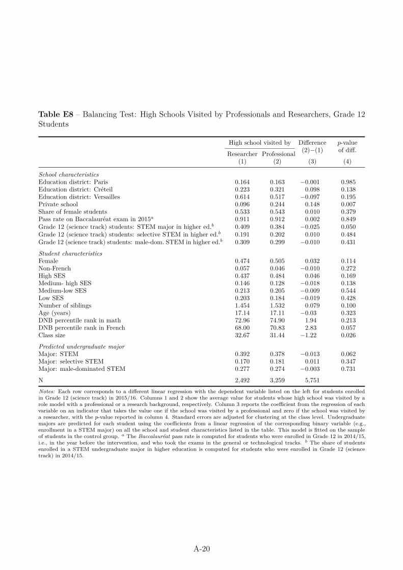
Table E8 – Balancing Test: High Schools Visited by Professionals and Researchers, Grade 12Students

High school visited by Difference(2)−(1)

p-valueof diff.Researcher Professional

(1) (2) (3) (4)

School characteristicsEducation district: Paris 0.164 0.163 −0.001 0.985Education district: Créteil 0.223 0.321 0.098 0.138Education district: Versailles 0.614 0.517 −0.097 0.195Private school 0.096 0.244 0.148 0.007Share of female students 0.533 0.543 0.010 0.379Pass rate on Baccalauréat exam in 2015a 0.911 0.912 0.002 0.849Grade 12 (science track) students: STEM major in higher ed.b 0.409 0.384 −0.025 0.050Grade 12 (science track) students: selective STEM in higher ed.b 0.191 0.202 0.010 0.484Grade 12 (science track) students: male-dom. STEM in higher ed.b 0.309 0.299 −0.010 0.431

Student characteristicsFemale 0.474 0.505 0.032 0.114Non-French 0.057 0.046 −0.010 0.272High SES 0.437 0.484 0.046 0.169Medium- high SES 0.146 0.128 −0.018 0.138Medium-low SES 0.213 0.205 −0.009 0.544Low SES 0.203 0.184 −0.019 0.428Number of siblings 1.454 1.532 0.079 0.100Age (years) 17.14 17.11 −0.03 0.323DNB percentile rank in math 72.96 74.90 1.94 0.213DNB percentile rank in French 68.00 70.83 2.83 0.057Class size 32.67 31.44 −1.22 0.026

Predicted undergraduate majorMajor: STEM 0.392 0.378 −0.013 0.062Major: selective STEM 0.170 0.181 0.011 0.347Major: male-dominated STEM 0.277 0.274 −0.003 0.731

N 2,492 3,259 5,751Notes: Each row corresponds to a different linear regression with the dependent variable listed on the left for students enrolledin Grade 12 (science track) in 2015/16. Columns 1 and 2 show the average value for students whose high school was visited by arole model with a professional or a research background, respectively. Column 3 reports the coefficient from the regression of eachvariable on an indicator that takes the value one if the school was visited by a professional and zero if the school was visited bya researcher, with the p-value reported in column 4. Standard errors are adjusted for clustering at the class level. Undergraduatemajors are predicted for each student using the coefficients from a linear regression of the corresponding binary variable (e.g.,enrollment in a STEM major) on all the school and student characteristics listed in the table. This model is fitted on the sampleof students in the control group. a The Baccalauréat pass rate is computed for students who were enrolled in Grade 12 in 2014/15,i.e., in the year before the intervention, and who took the exams in the general or technological tracks. b The share of studentsenrolled in a STEM undergraduate major in higher education is computed for students who were enrolled in Grade 12 (sciencetrack) in 2014/15.

A-20

F Effects of Role Model Interventions: Additional Re-sults

F.1 Student Perceptions

Table F1 – Gender Differences in Aptitude for Mathematics

Girls Boys

Controlgroupmean

Treatmenteffect

(LATE)

p-value[q-value]

Controlgroupmean

Treatmenteffect

(LATE)

p-value[q-value]

(1) (2) (3) (4) (5) (6)

Panel A. Grade 10

Equal gender aptitude for math (index) 0.115 0.109∗∗∗ 0.000 −0.134 0.148∗∗∗ 0.000(0.025) [0.001] (0.030) [0.001]

M and W are born with different brains 0.211 −0.050∗∗∗ 0.000 0.209 −0.048∗∗∗ 0.000(0.010) [0.001] (0.011) [0.001]

Men are more gifted in math than women 0.186 −0.026∗∗ 0.015 0.299 −0.048∗∗∗ 0.001(0.011) [0.016] (0.014) [0.001]

N 6,475 5,751

Panel B. Grade 12 (science track)

Equal gender aptitude for math (index) 0.158 0.095∗∗∗ 0.001 −0.161 0.132∗∗∗ 0.001(0.028) [0.002] (0.040) [0.002]

M and W are born with different brains 0.143 −0.023∗∗ 0.026 0.180 −0.038∗∗∗ 0.006(0.010) [0.026] (0.014) [0.013]

Men are more gifted in math than women 0.163 −0.038∗∗∗ 0.002 0.266 −0.028∗ 0.072(0.012) [0.005] (0.015) [0.073]

N 2,600 2,636

Notes: This table reports estimates of the treatment effects of the role model interventions on students’ perceptions regardingthe aptitude of men and women for mathematics, separately by grade level and gender. The sample is restricted to studentswho completed the post-intervention questionnaire. Each row corresponds to a different linear regression performed separately bygender, with the dependent variable listed on the left. Columns 1 and 4 report the average value for students in the control group.Columns 2 and 5 report the local average treatment effect (LATE) estimates. They are obtained from a regression of the outcome ofinterest on a classroom visit indicator, using treatment assignment as an instrument for treatment receipt. The regression controlsfor school fixed effects to account for the fact that randomization was stratified by school. Standard errors (shown in parentheses)are adjusted for clustering at the unit of randomization (class). Columns 3 and 6 report the cluster-robust p-value of the estimatedtreatment effect and, in square brackets, the p-value (q-value) adjusted for multiple hypotheses testing, using the False DiscoveryRate (FDR) control method. Specifically, we use the sharpened two-stage q-values introduced in Benjamini et al. (2006) anddescribed in Anderson (2008). The q-values associated with the synthetic index (highlighted in bold) are adjusted for multipletesting across the study’s nine main outcomes of interest, separately by grade level and gender (see Appendix D for details). Theq-values for the individual components of the index are adjusted for multiple testing across the index components, separately bygrade level and gender. *** p < 0.01, ** p < 0.05, * p < 0.1.

A-21

Table F2 – Taste for Science Subjects

Girls Boys

Controlgroupmean

Treatmenteffect

(LATE)

p-value[q-value]

Controlgroupmean

Treatmenteffect

(LATE)

p-value[q-value]

(1) (2) (3) (4) (5) (6)

Panel A. Grade 10

Taste for science subjects (index) −0.169 −0.038 0.294 0.197 −0.019 0.533(0.036) [0.442] (0.031) [0.685]

Enjoys math (z-score) −0.147 −0.002 0.961 0.186 −0.002 0.935(0.034) [0.961] (0.031) [0.935]

Enjoys physics-chemistry (z-score) −0.170 −0.040 0.289 0.223 −0.022 0.505(0.038) [0.578] (0.033) [0.935]

Enjoys earth and life sciences (z-score) −0.042 −0.058 0.137 0.086 −0.027 0.443(0.039) [0.548] (0.035) [0.935]

Enjoys science in general 0.661 −0.011 0.444 0.790 0.003 0.804(0.015) [0.593] (0.012) [0.935]

N 6,475 5,751

Panel B. Grade 12 (science track)

Taste for science subjects (index) −0.002 0.016 0.632 0.002 −0.000 0.998(0.034) [0.633] (0.039) [0.999]

Enjoys math (z-score) −0.097 0.067∗ 0.089 0.100 0.075∗ 0.063(0.040) [0.357] (0.040) [0.203]

Enjoys physics-chemistry (z-score) −0.089 −0.001 0.984 0.102 −0.021 0.598(0.044) [0.984] (0.040) [0.599]

Enjoys earth and life sciences (z-score) 0.203 −0.030 0.435 −0.215 −0.059 0.318(0.038) [0.871] (0.059) [0.424]

Enjoys science in general 0.918 −0.001 0.887 0.930 0.013 0.101(0.009) [0.984] (0.008) [0.203]

N 2,600 2,636Notes: This table reports estimates of the treatment effects of the role model interventions on students’ taste for science subjectstaught at school, separately by grade level and gender. The sample is restricted to students who completed the post-interventionquestionnaire. Each row corresponds to a different linear regression performed separately by gender, with the dependent variablelisted on the left. Columns 1 and 4 report the average value for students in the control group. Columns 2 and 5 report the localaverage treatment effect (LATE) estimates. They are obtained from a regression of the outcome of interest on a classroom visitindicator, using treatment assignment as an instrument for treatment receipt. The regression controls for school fixed effects toaccount for the fact that randomization was stratified by school. Standard errors (shown in parentheses) are adjusted for clusteringat the unit of randomization (class). Columns 3 and 6 report the cluster-robust p-value of the estimated treatment effect and,in square brackets, the p-value (q-value) adjusted for multiple hypotheses testing, using the False Discovery Rate (FDR) controlmethod. Specifically, we use the sharpened two-stage q-values introduced in Benjamini et al. (2006) and described in Anderson(2008). The q-values associated with the synthetic index (highlighted in bold) are adjusted for multiple testing across the study’snine main outcomes of interest, separately by grade level and gender (see Appendix D for details). The q-values for the individualcomponents of the index are adjusted for multiple testing across the index components, separately by grade level and gender.*** p < 0.01, ** p < 0.05, * p < 0.1.

A-22

Table F3 – Math Self-Concept

Girls Boys

Controlgroupmean

Treatmenteffect

(LATE)

p-value[q-value]

Controlgroupmean

Treatmenteffect

(LATE)

p-value[q-value]

(1) (2) (3) (4) (5) (6)

Panel A. Grade 10

Math self-concept (index) −0.198 −0.008 0.806 0.231 0.039 0.217(0.031) [0.807] (0.032) [0.326]

Self-assessed math performance (z-score) −0.127 −0.016 0.634 0.168 0.021 0.502(0.034) [0.634] (0.032) [0.642]

Lost in front of a math problem 0.553 0.010 0.478 0.344 −0.007 0.610(0.014) [0.634] (0.013) [0.642]

Worried when thinking about math 0.617 −0.025∗ 0.052 0.420 −0.032∗∗ 0.028(0.013) [0.109] (0.015) [0.111]

Can succeed in science subjects if puts in effort 0.843 0.018∗ 0.054 0.883 −0.004 0.642(0.009) [0.109] (0.008) [0.642]

N 6,475 5,751

Panel B. Grade 12 (science track)

Math self-concept (index) −0.184 0.050 0.202 0.187 0.072∗∗ 0.041(0.039) [0.228] (0.035) [0.062]

Self-assessed math performance (z-score) −0.126 0.039 0.304 0.123 0.079∗∗ 0.038(0.038) [0.406] (0.038) [0.077]

Lost in front of a math problem 0.486 −0.028 0.168 0.325 −0.028∗ 0.072(0.020) [0.336] (0.016) [0.096]

Worried when thinking about math 0.560 −0.037∗∗ 0.048 0.384 −0.051∗∗∗ 0.002(0.019) [0.193] (0.016) [0.007]

Can succeed in science subjects if puts in effort 0.942 −0.005 0.512 0.949 0.006 0.384(0.007) [0.512] (0.007) [0.385]

N 2,600 2,636Notes: This table reports estimates of the treatment effects of the role model interventions on students’ math self-concept, separatelyby grade level and gender. The sample is restricted to students who completed the post-intervention questionnaire. Each rowcorresponds to a different linear regression performed separately by gender, with the dependent variable listed on the left. Columns 1and 4 report the average value for students in the control group. Columns 2 and 5 report the local average treatment effect (LATE)estimates. They are obtained from a regression of the outcome of interest on a classroom visit indicator, using treatment assignmentas an instrument for treatment receipt. The regression controls for school fixed effects to account for the fact that randomizationwas stratified by school. Standard errors (shown in parentheses) are adjusted for clustering at the unit of randomization (class).Columns 3 and 6 report the cluster-robust p-value of the estimated treatment effect and, in square brackets, the p-value (q-value)adjusted for multiple hypotheses testing, using the False Discovery Rate (FDR) control method. Specifically, we use the sharpenedtwo-stage q-values introduced in Benjamini et al. (2006) and described in Anderson (2008). The q-values associated with thesynthetic index (highlighted in bold) are adjusted for multiple testing across the study’s nine main outcomes of interest, separatelyby grade level and gender (see Appendix D for details). The q-values for the individual components of the index are adjusted formultiple testing across the index components, separately by grade level and gender. *** p < 0.01, ** p < 0.05, * p < 0.1.

A-23

Table F4 – Science-Related Career Aspirations

Girls Boys

Controlgroupmean

Treatmenteffect

(LATE)

p-value[q-value]

Controlgroupmean

Treatmenteffect

(LATE)

p-value[q-value]

(1) (2) (3) (4) (5) (6)

Panel A. Grade 10

Science-related career aspirations (index) −0.103 0.012 0.695 0.120 0.007 0.801(0.030) [0.807] (0.029) [0.902]

Some jobs in science are interesting 0.845 0.019∗∗ 0.050 0.854 −0.000 1.000(0.009) [0.200] (0.010) [1.000]

Would consider a job in science 0.466 −0.004 0.776 0.587 0.023∗ 0.089(0.015) [0.776] (0.014) [0.358]

Interested in at least one STEM joba 0.642 0.005 0.696 0.849 0.013 0.181(0.013) [0.776] (0.010) [0.363]

Wage prospects important in career choice (z-score) −0.045 −0.012 0.682 0.038 0.007 0.792(0.029) [0.776] (0.027) [1.000]

N 6,475 5,751

Panel B. Grade 12 (science track)

Science-related career aspirations (index) −0.045 0.113∗∗∗ 0.002 0.046 0.050 0.131(0.037) [0.003] (0.033) [0.169]

Some jobs in science are interesting 0.961 0.013∗∗ 0.013 0.940 0.021∗∗∗ 0.005(0.005) [0.026] (0.008) [0.022]

Would consider a job in science 0.721 0.031∗∗ 0.019 0.762 0.030∗∗ 0.029(0.013) [0.026] (0.014) [0.058]

Interested in at least one STEM joba 0.817 0.000 0.964 0.899 −0.001 0.946(0.011) [0.964] (0.009) [0.947]

Wage prospects important in career choice (z-score) −0.043 0.119∗∗∗ 0.002 0.037 0.049 0.111(0.038) [0.007] (0.031) [0.149]

N 2,600 2,636Notes: This table reports estimates of the treatment effects of the role model interventions on students’ self-reported science-relatedcareer aspirations, separately by grade level and gender. The sample is restricted to students who completed the post-interventionquestionnaire. Each row corresponds to a different linear regression performed separately by gender, with the dependent variablelisted on the left. Columns 1 and 4 report the average value for students in the control group. Columns 2 and 5 report the localaverage treatment effect (LATE) estimates. They are obtained from a regression of the outcome of interest on a classroom visitindicator, using treatment assignment as an instrument for treatment receipt. The regression controls for school fixed effects toaccount for the fact that randomization was stratified by school. Standard errors (shown in parentheses) are adjusted for clusteringat the unit of randomization (class). Columns 3 and 6 report the cluster-robust p-value of the estimated treatment effect and,in square brackets, the p-value (q-value) adjusted for multiple hypotheses testing, using the False Discovery Rate (FDR) controlmethod. Specifically, we use the sharpened two-stage q-values introduced in Benjamini et al. (2006) and described in Anderson(2008). The q-values associated with the synthetic index (highlighted in bold) are adjusted for multiple testing across the study’snine main outcomes of interest, separately by grade level and gender (see Appendix D for details). The q-values for the individualcomponents of the index are adjusted for multiple testing across the index components, separately by grade level and gender.*** p < 0.01, ** p < 0.05, * p < 0.1. a The STEM occupations in the list were chemist, computer scientist, engineer, industrialdesigner, renewable energy technician, and researcher in biology. The non-STEM occupations were lawyer, pharmacist, physician,and psychologist.

A-24

F.2 Educational Choices

Table F5 – Grade 10 Students: Enrollment Status the Following Year (Detailed)

Grade 10 students

Girls Boys

Controlgroupmean

Treatmenteffect

(LATE)

p-value[q-value]

Controlgroupmean

Treatmenteffect

(LATE)

p-value[q-value]

(1) (2) (3) (4) (5) (6)

Panel A. Grade 11 STEM tracks

All STEM tracksScience track 0.355 −0.004 0.753 0.551 −0.002 0.910

(0.014) [0.807] (0.015) [0.910]

General vs. technological STEM trackScience - general track 0.328 0.001 0.942 0.416 0.007 0.613

(0.013) [0.942] (0.014) [0.614]

Science - technological track 0.026 −0.005 0.128 0.135 −0.009 0.300(0.003) [0.256] (0.008) [0.601]

Panel B. Grade 11 non-STEM tracks

All non-STEM tracksNon-STEM tracks 0.545 0.006 0.642 0.324 0.018 0.191

(0.014) (0.014)

General vs. technological non-STEM tracksHumanities track 0.121 −0.002 0.846 0.028 0.005 0.284

(0.010) (0.005)

Social sciences track 0.252 0.011 0.323 0.163 0.013 0.211(0.012) (0.010)

Non-STEM technological tracks 0.171 −0.003 0.759 0.133 0.001 0.944(0.010) (0.009)

Repeater or dropout 0.101 −0.002 0.818 0.126 −0.016∗ 0.070(0.009) (0.009)

N 7,241 6,459Notes: This table reports estimates of the treatment effects of the role model interventions on Grade 10 students’ enrollmentoutcomes in the academic year following the classroom interventions, i.e. 2016/17, separately by gender. The enrollment outcomesare measured using student-level administrative data. Each row corresponds to a different linear regression performed separately bygender, with the dependent variable listed on the left. Columns 1 and 4 report the average value for students in the control group.Columns 2 and 5 report the local average treatment effect (LATE) estimates. They are obtained from a regression of the outcomeof interest on a classroom visit indicator, using treatment assignment as an instrument for treatment receipt. The regressioncontrols for school fixed effects to account for the fact that randomization was stratified by school. Standard errors (shown inparentheses) are adjusted for clustering at the unit of randomization (class). Columns 3 and 6 report the cluster-robust p-valueof the estimated treatment effect and, in square brackets, the p-value (q-value) adjusted for multiple hypotheses testing, using theFalse Discovery Rate (FDR) control method. Specifically, we use the sharpened two-stage q-values introduced in Benjamini et al.(2006) and described in Anderson (2008). The q-values associated with the treatment effect estimates on the probability of beingenrolled in the science track in Grade 11 (Panel A) are adjusted for multiple testing across the study’s nine main outcomes ofinterest, separately by gender (see Appendix D for details). The q-values associated with the treatment effect estimates for thedifferent STEM tracks (general vs. technological) are adjusted for multiple testing across these two tracks, separately by gender.*** p < 0.01, ** p < 0.05, * p < 0.1.

A-25

Table F6 – Grade 12 Students: Enrollment Status the Following Year (Detailed)

Grade 12 (science track) students

Girls Boys

Controlgroupmean

Treatmenteffect

(LATE)

p-value[q-value]

Controlgroupmean

Treatmenteffect

(LATE)

p-value[q-value]

(1) (2) (3) (4) (5) (6)

Panel A. STEM undergraduate programs

All undergraduate STEM majorsMajor: STEM 0.289 0.024∗ 0.080 0.470 0.003 0.886

(0.014) [0.103] (0.020) [0.988]

Selective STEM majorsMath, physics, engineering, computer science (CPGE) 0.084 0.026∗∗∗ 0.006 0.211 0.023 0.123

(0.009) [0.032] (0.015) [0.206]

Earth and life sciences (CPGE) 0.020 0.008 0.137 0.010 0.002 0.617(0.005) [0.230] (0.003) [0.771]

Sciences - vocational (STS) 0.006 0.002 0.474 0.011 −0.005 0.110(0.003) [0.474] (0.003) [0.206]

Non-selective STEM majorsMath, physics, computer science 0.077 0.010 0.209 0.157 −0.002 0.884

(0.008) [0.262] (0.012) [0.885]

Earth and life sciences 0.103 −0.022∗∗ 0.014 0.081 −0.015∗ 0.053(0.009) [0.035] (0.008) [0.206]

Panel B. Non-STEM undergraduate programs

All undergraduate non-STEM majorsMajor: non-STEM 0.507 −0.032∗∗ 0.045 0.293 −0.005 0.717

(0.016) (0.014)

Selective non-STEM majorsBusiness and economics (CPGE) 0.021 0.003 0.566 0.017 0.005 0.219

(0.004) (0.004)

Humanities (CPGE) 0.014 −0.004 0.225 0.003 −0.001 0.470(0.003) (0.001)

Other vocational (STS) 0.011 −0.008∗∗∗ 0.006 0.008 −0.005∗∗ 0.036(0.003) (0.002)

Non-selective non-STEM majorsMedicine and pharmacy 0.259 −0.005 0.722 0.108 0.006 0.573

(0.015) (0.011)

Law and economics 0.107 −0.008 0.478 0.079 0.002 0.758(0.011) (0.008)

Humanities and psychology 0.080 −0.008 0.339 0.040 −0.006 0.296(0.009) (0.006)

Sports studies 0.018 −0.004 0.396 0.036 −0.005 0.377(0.004) (0.006)

Not enrolled in higher education 0.206 0.008 0.581 0.237 0.004 0.814(0.015) (0.016)

N 2,827 2,924

Notes: This table reports estimates of the treatment effects of the role model interventions on science track Grade 12 (science track)students’ enrollment outcomes in the academic year following the classroom interventions, i.e. 2016/17, separately by gender. Theenrollment outcomes are measured using student-level administrative data. Each row corresponds to a different linear regressionperformed separately by gender, with the dependent variable listed on the left. Columns 1 and 4 report the average value for studentsin the control group. Columns 2 and 5 report the local average treatment effect (LATE) estimates. They are obtained from aregression of the outcome of interest on a classroom visit indicator, using treatment assignment as an instrument for treatmentreceipt. The regression controls for school fixed effects to account for the fact that randomization was stratified by school. Standarderrors (shown in parentheses) are adjusted for clustering at the unit of randomization (class). Columns 3 and 6 report the cluster-robust p-value of the estimated treatment effect and, in square brackets, the p-value (q-value) adjusted for multiple hypothesestesting, using the False Discovery Rate (FDR) control method. Specifically, we use the sharpened two-stage q-values introducedin Benjamini et al. (2006) and described in Anderson (2008). The q-values associated with the treatment effect estimates on theprobability of enrolling in a STEM undergraduate major (Panel A) are adjusted for multiple testing across the study’s nine mainoutcomes of interest, separately by gender (see Appendix D for details). The q-values associated with the estimates for the differentselective and non-selective STEM majors (Panel A) are adjusted for multiple testing across these different STEM majors, separatelyby gender. *** p < 0.01, ** p < 0.05, * p < 0.1.

A-26

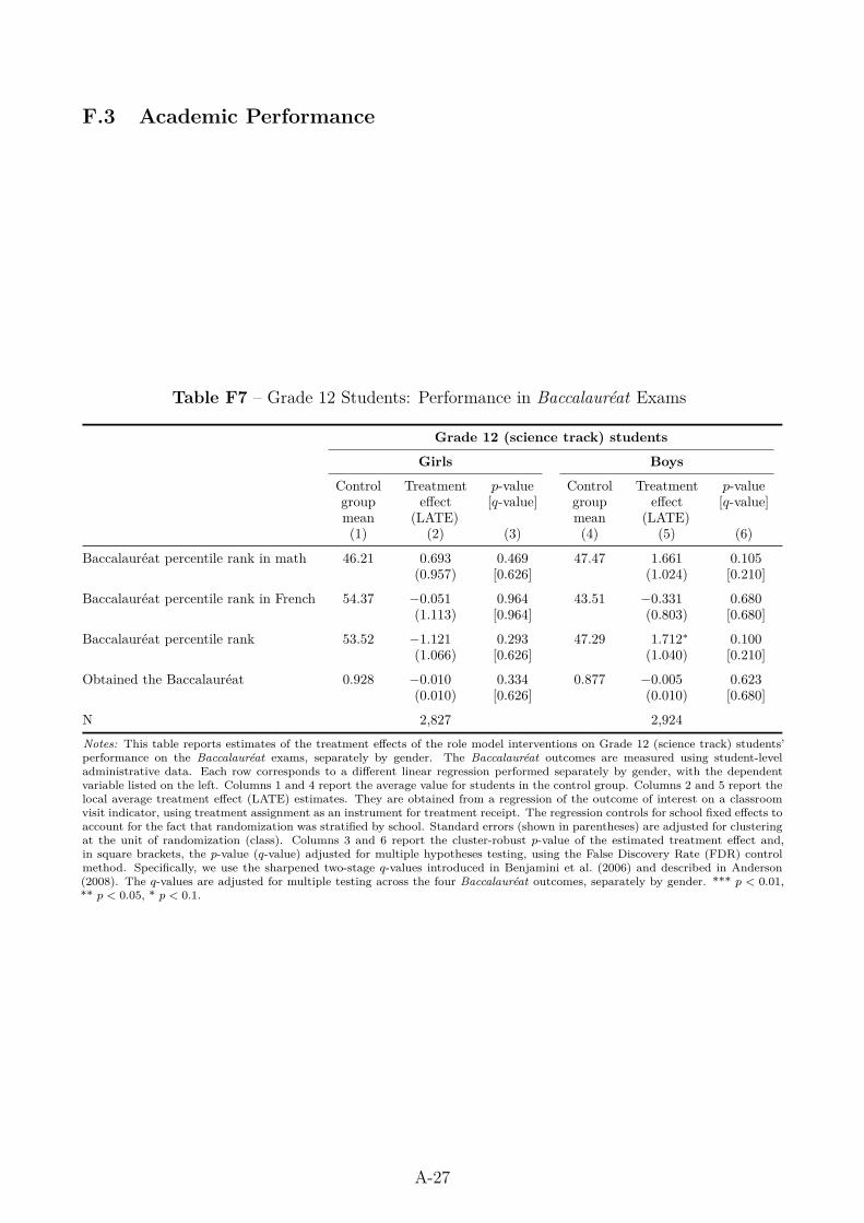
F.3 Academic Performance

Table F7 – Grade 12 Students: Performance in Baccalauréat Exams

Grade 12 (science track) students

Girls Boys

Controlgroupmean

Treatmenteffect

(LATE)

p-value[q-value]

Controlgroupmean

Treatmenteffect

(LATE)

p-value[q-value]

(1) (2) (3) (4) (5) (6)

Baccalauréat percentile rank in math 46.21 0.693 0.469 47.47 1.661 0.105(0.957) [0.626] (1.024) [0.210]

Baccalauréat percentile rank in French 54.37 −0.051 0.964 43.51 −0.331 0.680(1.113) [0.964] (0.803) [0.680]

Baccalauréat percentile rank 53.52 −1.121 0.293 47.29 1.712∗ 0.100(1.066) [0.626] (1.040) [0.210]

Obtained the Baccalauréat 0.928 −0.010 0.334 0.877 −0.005 0.623(0.010) [0.626] (0.010) [0.680]

N 2,827 2,924Notes: This table reports estimates of the treatment effects of the role model interventions on Grade 12 (science track) students’performance on the Baccalauréat exams, separately by gender. The Baccalauréat outcomes are measured using student-leveladministrative data. Each row corresponds to a different linear regression performed separately by gender, with the dependentvariable listed on the left. Columns 1 and 4 report the average value for students in the control group. Columns 2 and 5 report thelocal average treatment effect (LATE) estimates. They are obtained from a regression of the outcome of interest on a classroomvisit indicator, using treatment assignment as an instrument for treatment receipt. The regression controls for school fixed effects toaccount for the fact that randomization was stratified by school. Standard errors (shown in parentheses) are adjusted for clusteringat the unit of randomization (class). Columns 3 and 6 report the cluster-robust p-value of the estimated treatment effect and,in square brackets, the p-value (q-value) adjusted for multiple hypotheses testing, using the False Discovery Rate (FDR) controlmethod. Specifically, we use the sharpened two-stage q-values introduced in Benjamini et al. (2006) and described in Anderson(2008). The q-values are adjusted for multiple testing across the four Baccalauréat outcomes, separately by gender. *** p < 0.01,** p < 0.05, * p < 0.1.

A-27

G Robustness Checks

Table G1 – Treatment Effects on Student Perceptions: Controlling for Baseline Characteristics

Girls Boys

Controlgroupmean

Treatmenteffect

(LATE)

p-value[q-value]

Controlgroupmean

Treatmenteffect

(LATE)

p-value[q-value]

(1) (2) (3) (4) (5) (6)

Panel A. Grade 10

Positive perceptions of science-related careers (index) −0.020 0.245∗∗∗ 0.000 0.023 0.162∗∗∗ 0.000(0.027) [0.001] (0.027) [0.001]

More men in science-related jobs 0.628 0.154∗∗∗ 0.000 0.629 0.170∗∗∗ 0.000(0.013) [0.001] (0.014) [0.001]

Equal gender aptitude for math (index) 0.115 0.111∗∗∗ 0.000 −0.134 0.142∗∗∗ 0.000(0.024) [0.001] (0.030) [0.001]

Women don’t really like science 0.157 0.056∗∗∗ 0.000 0.198 0.101∗∗∗ 0.000(0.011) [0.001] (0.013) [0.001]

W face discrimination in science-related jobs 0.603 0.126∗∗∗ 0.000 0.527 0.154∗∗∗ 0.000(0.013) [0.001] (0.014) [0.001]

Taste for science subjects (index) −0.169 −0.033 0.275 0.197 −0.021 0.431(0.031) [0.414] (0.026) [0.555]

Math self-concept (index) −0.198 −0.001 0.981 0.231 0.033 0.250(0.028) [0.982] (0.029) [0.375]

Science-related careers aspirations (index) −0.103 0.005 0.851 0.120 0.004 0.871(0.029) [0.970] (0.027) [0.872]

N 6,475 5,751

Panel B. Grade 12 (science track)

Positive perceptions of science-related careers (index) −0.003 0.296∗∗∗ 0.000 0.003 0.171∗∗∗ 0.000(0.032) [0.001] (0.033) [0.001]

More men in science-related jobs 0.712 0.122∗∗∗ 0.000 0.717 0.149∗∗∗ 0.000(0.016) [0.001] (0.015) [0.001]

Equal gender aptitude for math (index) 0.158 0.078∗∗∗ 0.004 −0.161 0.124∗∗∗ 0.003(0.028) [0.007] (0.042) [0.006]

Women don’t really like science 0.074 0.042∗∗∗ 0.000 0.146 0.073∗∗∗ 0.000(0.009) [0.001] (0.015) [0.001]

W face discrimination in science-related jobs 0.624 0.085∗∗∗ 0.000 0.600 0.074∗∗∗ 0.000(0.020) [0.001] (0.018) [0.001]

Taste for science subjects (index) −0.002 0.018 0.583 0.002 0.014 0.733(0.033) [0.583] (0.040) [0.825]

Math self-concept (index) −0.184 0.051 0.139 0.187 0.068∗∗ 0.038(0.035) [0.157] (0.033) [0.057]

Science-related careers aspirations (index) −0.045 0.106∗∗∗ 0.004 0.046 0.068∗ 0.055(0.037) [0.007] (0.035) [0.071]

N 2,600 2,636

Notes: This table reports estimates of the treatment effects of the role model interventions on students’ perceptions, separately bygrade level and gender, and controlling for students’ baseline characteristics. The sample is restricted to students who completedthe post-intervention questionnaire. Each row corresponds to a different linear regression performed separately by gender, withthe dependent variable listed on the left. Columns 1 and 4 report the average value for students in the control group. Columns 2and 5 report the local average treatment effect (LATE) estimates. They are obtained from a regression of the outcome of intereston a classroom visit indicator, using treatment assignment as an instrument for treatment receipt. The regression controls forschool fixed effects to account for the fact that randomization was stratified by school. The regression further controls for thestudent characteristics listed in Table 1 in the main text. Standard errors (shown in parentheses) are adjusted for clustering at theunit of randomization (class). Columns 3 and 6 report the cluster-robust p-value of the estimated treatment effect and, in squarebrackets, the p-value (q-value) adjusted for multiple hypotheses testing, using the False Discovery Rate (FDR) control method.Specifically, we use the sharpened two-stage q-values introduced in Benjamini et al. (2006) and described in Anderson (2008). Theq-values are adjusted for multiple testing across the study’s nine main outcomes of interest, separately by grade level and gender(see Appendix D for details). *** p < 0.01, ** p < 0.05, * p < 0.1.

A-28

Table G2 – Treatment Effects on Enrollment Outcomes: Controlling for Baseline Characteristics

Girls Boys

Controlgroupmean

Treatmenteffect

(LATE)

p-value[q-value]

Controlgroupmean

Treatmenteffect

(LATE)

p-value[q-value]

(1) (2) (3) (4) (5) (6)

Panel A. Grade 10

All STEM tracksGrade 11: Science track 0.355 −0.002 0.862 0.551 −0.006 0.640

(0.011) [0.970] (0.012) [0.720]

General vs. technological STEM trackGrade 11: Science - general track 0.328 0.003 0.794 0.416 0.004 0.710

(0.010) [0.794] (0.011) [0.710]

Grade 11: Science - technological track 0.026 −0.005 0.188 0.135 −0.010 0.234(0.004) [0.377] (0.008) [0.468]

N 7,241 6,459

Panel B. Grade 12 (science track)

All undergraduate STEM majorsMajor: STEM 0.289 0.020 0.139 0.470 −0.002 0.925

(0.014) [0.157] (0.019) [0.926]

Selective vs. non-selective STEMMajor: selective STEM 0.110 0.031∗∗∗ 0.006 0.232 0.008 0.575

(0.011) [0.012] (0.015) [0.575]

Major: non-selective STEM 0.178 −0.011 0.333 0.239 −0.010 0.445(0.012) [0.333] (0.013) [0.575]

Male- vs. female-dominated STEMMajor: male-dominated STEM 0.166 0.034∗∗∗ 0.004 0.379 0.013 0.485(math, physics, computer science) (0.012) [0.012] (0.019) [0.575]

Major: female-dominated STEM 0.123 −0.015 0.169 0.091 −0.015 0.119(earth and life sciences) (0.011) [0.226] (0.009) [0.477]

N 2,827 2,924Notes: This table reports estimates of the treatment effects of the role model interventions on students’ enrollment outcomes in theacademic year following the classroom interventions, i.e., 2016/17, separately by grade level and gender, and controlling for studentbaseline characteristics. The enrollment outcomes are measured using student-level administrative data. Each row corresponds toa different linear regression performed separately by gender, with the dependent variable listed on the left. Columns 1 and 4 reportthe average value for students in the control group. Columns 2 and 5 report the local average treatment effect (LATE) estimates.They are obtained from a regression of the outcome of interest on a classroom visit indicator, using treatment assignment as aninstrument for treatment receipt. The regression controls for school fixed effects to account for the fact that randomization wasstratified by school. The regression further controls for the student characteristics listed in Table 1 in the main text. Standarderrors (shown in parentheses) are adjusted for clustering at the unit of randomization (class). Columns 3 and 6 report the cluster-robust p-value of the estimated treatment effect and, in square brackets, the p-value (q-value) adjusted for multiple hypothesestesting, using the False Discovery Rate (FDR) control method. Specifically, we use the sharpened two-stage q-values introduced inBenjamini et al. (2006) and described in Anderson (2008). The q-values associated with the treatment effect estimates on “Grade 11:Science track” (Panel A) and “Major: STEM” (Panel B) are adjusted for multiple testing across the study’s nine main outcomesof interest, separately by grade level and gender (see Appendix D for details). The q-values associated with the treatment effectestimates for the different STEM tracks (Panel A) or the different STEM majors (Panel B) are adjusted for multiple testing acrossthese different STEM tracks or majors, separately by grade level and gender. *** p < 0.01, ** p < 0.05, * p < 0.1.

A-29

H Randomization InferenceThis appendix evaluates the robustness of our results to computing p-values using non-parametricrandomization inference tests rather than model-based cluster-robust inference.

Randomization inference, which was first proposed by Fisher (1935) and was later developedby Rosenbaum (2002), has been used in a number of recent RCT studies in economics andpolitical science as an alternative to model-based inference The intuition behind this approachis relatively straightforward. In RCTs, researchers know exactly how the randomization wasperformed. Randomization inference uses this knowledge to assess whether observed outcomesin a given sample are likely to have occurred by chance even if the treatment had no effect.This can be obtained numerically through Monte Carlo methods, by computing the treatmenteffects for varying random draws of the treatment assignment, whose data-generating process isknown. This test is non-parametric since it does not make distributional assumptions.A.5

In our setting, the ITT effect under the observed assignment to treatment is estimated usingthe following reduced-form specification:

Yics = α + βTcs + θs + εics, (A.1)

where Yics denotes the observed outcome of student i in class c and high school s; Tcs denotesthe observed treatment assignment of the student’s class; and θs are school fixed effects. TheITT estimate under the observed treatment assignment is denoted by β.

To conduct randomization inference, we proceed as follows. Taking into account thefact that randomization was stratified by school and grade level, we first re-assign treatmentR =2,000 times among participating classes using the exact same stratified procedure.A.6 Let{P r}Rr=1 denote the set of R random placebo assignments from the randomization process. Wethen re-estimate the ITT effects of these placebo treatments using the following reduced-formspecification, which is estimated separately by grade level and gender:

Yics = αr + βrPrcs + λs + ηics, r = 1, ..., R, (A.2)

where P rcs indicates assignment to a placebo treatment group for random draw r. School fixed

effects, λs, are included to account for the fact that the randomization is stratified by school.Since Pr is a randomly generated placebo, E(βr) = 0. Let F (βr) denote the empirical c.d.f. of

all elements of {Pr}Rr=1. We test the null hypothesis that the program had no effect on outcome Yby checking if the ITT estimate that we obtain for the observed treatment assignment is in thetails of the distribution of placebo treatments. We can reject H0: β = 0 with a confidence levelof 1− α if β ≤ F−1

(α2

)or β ≥ F−1

(1− α

2

). Since the placebo assignments only vary across

randomization units (here classes), this method accounts for correlation within units. FollowingDavison and Hinkley (1997), we compute the p-values from a two-sided randomization inferencetest of zero treatment effects as p = (1 +∑R

r=1 1(|βr| ≥ |β|))/(1 +R).Table H1 presents the results of randomization inference tests of the hypotheses that the role

model interventions had no effect on student perceptions and enrollment outcomes, separately bygrade level and gender. The ITT estimates β are shown in columns 1 and 4. The cluster-robustmodel-based p-values are reported and columns 2 and 5, while those based on randomizationinference are in columns 3 and 6. The results of the randomization inference tests yield p-valuesthat are generally close to the cluster-robust model-based p-values. Although they tend tobe slightly more conservative, they confirm the program’s statistically significant effects onenrollment in selective and male-dominated STEM programs for girls in Grade 12.

A.5For more details on randomization inference, see Rosenbaum (2010) and Imbens and Rubin (2015).A.6See Paz and West (2019) for the number of draws to be used.

A-30

Table H1 – Randomization Inference for Intention-to-Treat Estimates

Girls Boys

ITT p-value:model-based

p-value:rand.

inference

ITT p-value:model-based

p-value:rand.

inference

(1) (2) (3) (4) (5) (6)

Panel A. Grade 10

Student perceptionsPositive perceptions of science-related careers (index) 0.226 0.000 0.000 0.156 0.000 0.000More men in science-related jobs 0.145 0.000 0.000 0.157 0.000 0.000Equal gender aptitude for math (index) 0.101 0.000 0.000 0.138 0.000 0.000Women don’t really like science 0.054 0.000 0.000 0.096 0.000 0.000Women face discrimination in science-related careers 0.118 0.000 0.000 0.143 0.000 0.000Taste for science subjects (index) −0.035 0.298 0.340 −0.018 0.537 0.560Math self-concept (index) −0.007 0.808 0.820 0.037 0.221 0.280Science-related career aspirations (index) 0.011 0.697 0.720 0.007 0.803 0.830

Enrollment outcomesGrade 11: Science track −0.004 0.755 0.780 −0.002 0.911 0.920Grade 11: Science - general track 0.001 0.942 0.950 0.007 0.617 0.660Grade 11: Science - technological track −0.005 0.131 0.190 −0.008 0.306 0.350

N 7,241 6,459

Panel B. Grade 12 (science track)

Student perceptionsPositive perceptions of science-related careers (index) 0.293 0.000 0.000 0.145 0.000 0.000More men in science-related jobs 0.118 0.000 0.000 0.140 0.000 0.000Equal gender aptitude for math (index) 0.090 0.001 0.020 0.124 0.002 0.020Women don’t really like science 0.042 0.000 0.000 0.069 0.000 0.000Women face discrimination in science-related careers 0.090 0.000 0.000 0.068 0.000 0.000Taste for science subjects (index) 0.015 0.640 0.740 −0.000 0.998 1.000Math self-concept (index) 0.047 0.214 0.360 0.068 0.044 0.140Science-related career aspirations (index) 0.106 0.003 0.020 0.047 0.141 0.270

Enrollment outcomesUndergraduate major: STEM 0.022 0.091 0.220 0.003 0.889 0.920Undergraduate major: selective STEM 0.033 0.002 0.030 0.019 0.208 0.360Undergraduate major: non-selective STEM −0.010 0.328 0.480 −0.016 0.220 0.370Undergraduate major: male-dominated STEM 0.035 0.002 0.020 0.016 0.397 0.530Undergraduate major: female-dominated STEM −0.014 0.162 0.320 −0.013 0.128 0.270

N 2,827 2,924Notes: This table presents the results of randomization inference tests of the hypotheses that the program had no effect on studentperceptions and enrollment outcomes. We randomly re-assign treatment 2,000 times among participating classes within each schooland grade level, and re-estimate the ITT effects of these placebo treatments. The ITT estimates under the observed assignmentare reported in columns 1 and 4 separately by gender. The associated cluster-robust model-based p-values are shown in columns 2and 5. The randomization inference p-values are reported in columns 3 and 6. They are computed from a two-sided randomizationinference test of zero treatment effects as p =

(1 +∑R

r=1 1(|βr| ≥ |β|))/(1 + R), where {βr}R

r=1 is the set of R placebo ITTestimates, β is the ITT estimate under the observed assignment, and 1(·) is the indicator function.

A-31

I Information, Persistence, Timing: Additional Results

I.1 Intensity of Information Provision

Figure I1 – Screenshots of the Slides Providing General Information on STEM Careers (“RegularSlides”)

Figure I2 – Screenshots of the Additional Slides Providing General Information on STEMCareers (“Augmented Slides”)

A-32

Table I1 – Balancing Test: Classrooms Assigned to Role Models who were Provided with theRegular vs. Augmented Sets of Slides

Set of slides Difference(2)−(1)

p-valueof diff.Regular Augmented

(1) (2) (3) (4)

Panel A. Grade 10

Student characteristicsGirl 0.532 0.526 −0.006 0.651Non-French 0.052 0.067 0.015 0.014High SES 0.396 0.369 −0.027 0.193Medium- high SES 0.136 0.122 −0.014 0.059Medium-low SES 0.238 0.244 0.006 0.559Low SES 0.229 0.265 0.035 0.030Number of siblings 1.467 1.500 0.033 0.383At least one science elective course 0.387 0.399 0.012 0.722At least one standard elective course 0.746 0.759 0.012 0.648Age (years) 15.10 15.14 0.04 0.002DNB percentile rank in math 58.37 58.57 0.20 0.886DNB percentile rank in French 56.79 58.69 1.90 0.122Number of classmates 33.86 32.76 −1.10 0.000

Predicted track in Grade 11Grade 11: Science track 0.443 0.457 0.014 0.248Grade 11: Science - general track 0.366 0.380 0.014 0.326Grade 11: Science - technical track 0.077 0.077 0.000 0.923

N 6,047 7,653 13,700

Panel B. Grade 12 (science track)

Student characteristicsGirl 0.491 0.492 0.001 0.951Non-French 0.044 0.057 0.014 0.133High SES 0.475 0.453 −0.022 0.519Medium- high SES 0.140 0.132 −0.008 0.517Medium-low SES 0.209 0.208 −0.001 0.936Low SES 0.176 0.207 0.031 0.197Number of siblings 1.479 1.516 0.037 0.454Age (years) 17.12 17.13 0.01 0.673DNB percentile rank in math 74.19 73.94 −0.25 0.870DNB percentile rank in French 69.45 69.75 0.30 0.843Number of classmates 32.13 31.83 −0.29 0.602

Predicted undergraduate majorMajor: STEM 0.384 0.382 −0.002 0.735Undergraduate major: male-dominated STEM 0.276 0.274 −0.001 0.856Undergraduate major: selective STEM 0.179 0.175 −0.004 0.684

N 2,748 3,003 5,751Notes: Each row corresponds to a different linear regression with the dependent variable listed on the left for students enrolled inGrade 10 in 2015/16 (Panel A) and in Grade 12 (Panel B). Columns 1 and 2 show the average value for students whose high schoolwas visited by a role model provided with the regular or augmented set of slides, respectively. Column 3 reports the coefficientfrom the regression of each variable on an indicator that takes the value one if the school was visited by a role model who receivedthe augmented slides and zero if the school was visited by a role model who received the regular slides, with the p-value reportedin column 4. Standard errors are adjusted for clustering at the class level. High school tracks in Grade 11 are predicted for eachstudent using the coefficients from a linear regression of the corresponding binary variable (e.g., enrollment in the general sciencetrack) on all the student characteristics listed in the table. This model is fitted on the sample of students in the control group.

A-33

Table I2 – Treatment Effects (ITT) for Grade 12 Students: Regular vs. Augmented Slides

Girls Boys

(1) (2) (3) (4)

Major: STEM

Treatment group indicator (T ) 0.022 0.003 0.013 0.007(0.019) (0.021) (0.030) (0.031)

T*Augmented slides 0.001 0.036 −0.018 0.008(0.026) (0.031) (0.037) (0.042)

Undergraduate major: male-dominated STEM

Treatment group indicator (T ) 0.044∗∗∗ 0.030∗ 0.017 0.007(0.016) (0.018) (0.031) (0.030)

T*Augmented slides −0.015 0.006 −0.002 0.024(0.023) (0.026) (0.037) (0.040)

Undergraduate major: selective STEM

Treatment group indicator (T ) 0.041∗∗ 0.033∗ 0.025 0.018(0.017) (0.017) (0.024) (0.025)

T*Augmented slides −0.018 −0.001 −0.012 0.010(0.022) (0.024) (0.030) (0.035)

Science-related jobs pay higher wages

Treatment group indicator (T ) 0.005 0.017 0.003 0.040∗(0.026) (0.031) (0.023) (0.021)

T*Augmented slides 0.097∗∗∗ 0.069 0.041 −0.040(0.034) (0.044) (0.031) (0.030)

Positive perceptions of science-related careers (index)

Treatment group indicator (T ) 0.254∗∗∗ 0.294∗∗∗ 0.154∗∗∗ 0.184∗∗∗(0.055) (0.054) (0.046) (0.048)

T*Augmented slides 0.078 0.022 −0.013 −0.061(0.069) (0.077) (0.064) (0.077)

Equal aptitudes of M and W for science (index)

Treatment group indicator (T ) 0.060 0.077∗ 0.060 0.054(0.038) (0.042) (0.049) (0.055)

T*Augmented slides 0.056 0.026 0.112 0.117(0.055) (0.064) (0.074) (0.085)

Month of Visit FE No Yes No Yes

Month of Visit FE * treatment group indicator No Yes No Yes

N 2,827 2,827 2,924 2,924

Notes: This table reports estimates of the treatment effects (ITT) of the role model interventions on student outcomes for Grade 12students, separately by gender and by the type of slides (regular or augmented) that were provided to the female role model whovisited the classroom. For each outcome of interest, the reported coefficients are obtained from a regression of the outcome ofinterest on a treatment group indicator (T ) and the interaction between this indicator and an indicator that takes the value one ifthe role model was provided with the augmented set of slides. The specification in columns 1 and 3 includes school fixed effects toaccount for the fact that randomization was stratified by school. Columns 2 and 4 further include month-of-visit fixed effects toaccount for the fact that the additional slides were provided slightly later in the experiment. Standard errors (shown in parentheses)are adjusted for clustering at the unit of randomization (class). *** p < 0.01, ** p < 0.05, * p < 0.1.

A-34

I.2 Persistence of the Effects and Timing of Visits

Table I3 – Persistence of Effects on Student Perceptions

Girls BoysMonths since intervention Months since intervention1 to 2months

3 to 4months

5 to 6months

1 to 2months

3 to 4months

5 to 6months

(1) (2) (3) (4) (5) (6)Panel A. Grade 10Positive perceptions of science-related careers (index) 0.413∗∗∗ 0.200∗∗∗ 0.143∗ 0.192∗∗∗ 0.168∗∗∗ 0.049

(0.057) (0.037) (0.077) (0.053) (0.036) (0.083)More men in science-related jobs 0.170∗∗∗ 0.154∗∗∗ 0.164∗∗∗ 0.209∗∗∗ 0.163∗∗∗ 0.116∗∗∗

(0.021) (0.017) (0.033) (0.022) (0.018) (0.039)Equal gender aptitude for math (index) 0.179∗∗∗ 0.101∗∗∗ 0.019 0.244∗∗∗ 0.122∗∗∗ 0.090

(0.047) (0.032) (0.065) (0.053) (0.040) (0.069)Women don’t really like science 0.047∗∗ 0.067∗∗∗ 0.041 0.131∗∗∗ 0.107∗∗∗ 0.017

(0.022) (0.014) (0.026) (0.020) (0.016) (0.040)W face discrimination in science-related careers 0.158∗∗∗ 0.135∗∗∗ 0.081∗∗ 0.162∗∗∗ 0.174∗∗∗ 0.110∗∗∗

(0.022) (0.017) (0.039) (0.026) (0.017) (0.036)Taste for science subjects (index) 0.088 −0.035 −0.053 0.043 −0.008 0.043

(0.075) (0.043) (0.075) (0.058) (0.041) (0.072)Math self-concept (index) −0.029 0.006 0.044 −0.041 0.103∗∗∗ 0.088

(0.057) (0.039) (0.080) (0.063) (0.039) (0.090)Science-related career aspirations (index) 0.088 −0.002 0.010 −0.000 0.022 0.010

(0.057) (0.036) (0.062) (0.051) (0.038) (0.072)N 1,729 3,716 831 1,677 3,318 693Panel B. Grade 12 (science track)Positive perceptions of science-related careers (index) 0.442∗∗∗ 0.253∗∗∗ 0.353∗∗∗ 0.182∗∗∗ 0.169∗∗∗ 0.003

(0.053) (0.043) (0.118) (0.061) (0.044) (0.095)More men in science-related jobs 0.128∗∗∗ 0.107∗∗∗ 0.208∗∗∗ 0.114∗∗∗ 0.159∗∗∗ 0.208∗∗∗

(0.031) (0.019) (0.060) (0.023) (0.021) (0.046)Equal gender aptitude for math (index) 0.077 0.138∗∗∗ 0.020 0.218∗∗∗ 0.106∗∗ 0.044

(0.067) (0.033) (0.094) (0.081) (0.051) (0.123)Women don’t really like science 0.067∗∗∗ 0.040∗∗∗ 0.032∗ 0.042 0.077∗∗∗ 0.144∗∗∗

(0.021) (0.011) (0.018) (0.029) (0.019) (0.032)W face discrimination in science-related jobs 0.104∗∗∗ 0.102∗∗∗ 0.087 0.083∗∗∗ 0.085∗∗∗ −0.011

(0.038) (0.023) (0.072) (0.027) (0.024) (0.062)Taste for science subjects (index) −0.063 −0.028 0.258∗∗∗ 0.030 0.010 −0.090

(0.071) (0.045) (0.060) (0.079) (0.049) (0.111)Math self-concept (index) 0.043 0.001 0.169 −0.022 0.114∗∗ 0.126

(0.065) (0.053) (0.122) (0.054) (0.046) (0.149)Science-related career aspirations (index) −0.005 0.123∗∗∗ 0.231∗∗∗ 0.007 0.048 0.098

(0.077) (0.045) (0.077) (0.046) (0.046) (0.118)N 689 1,468 394 717 1,514 370Notes: This table reports estimates of the treatment effects of the role model interventions on student perceptions, separatelyby grade level, gender, and intervals of elapsed time between the classroom intervention and the student survey. The sample isrestricted to students who completed the post-intervention questionnaire. Each coefficient is obtained from a linear regression ofthe outcome of interest on a classroom visit indicator, using treatment assignment as an instrument for treatment receipt. Theregression controls for school fixed effects to account for the fact that randomization was stratified by school. Standard errors(shown in parentheses) are adjusted for clustering at the unit of randomization (class).

A-35

(a) Enrollment in selective STEM

0%

20%

40%

60%

All Nov Dec Jan Feb/MarMonth of classroom intervention

Girls

0%

20%

40%

60%

All Nov Dec Jan Feb/MarMonth of classroom intervention

Boys

Control group mean Control group mean + treatment effect 95% CI

(b) Enrollment in male-dominated STEM

0%

20%

40%

60%

All Nov Dec Jan Feb/MarMonth of classroom intervention

Girls

0%

20%

40%

60%

All Nov Dec Jan Feb/MarMonth of classroom intervention

Boys

Control group mean Control group mean + treatment effect 95% CI

Figure I3 – Grade 12 Students: Enrollment in Selective and Male-Dominated STEM Under-graduate Programs, by Gender and Month of Classroom InterventionNotes: The figure shows the fraction of Grade 12 (science track) students who enrolled in selective (Panel A) and in male-dominated(Panel B) STEM undergraduate programs after graduating for high school, separately for girls (left panel) and for boys (right panel).The filled bars indicate the baseline enrollment rates among students in the control group, both overall and separately by monthof classroom intervention. The solid dots show the estimated treatment effects (added to the control group means) with 95 percentconfidence intervals denoted by vertical capped bars. The treatment effects are estimated from separate regressions of the outcomeof interest on a classroom visit indicator, using treatment assignment as an instrument for treatment receipt. The regressioncontrols for school fixed effects to account for the fact that randomization was stratified by school. Standard errors are adjustedfor clustering at the unit of randomization (class).

A-36

J Spillover EffectsThis appendix investigates whether the program could have had spillover effects for studentswho were not exposed to the role model interventions in participating schools. Section J.1provides survey evidence suggesting that the scope for spillover effects was relatively limited.Section J.2 describes the difference-in-differences (DiD) approach that we use to estimate themagnitude of spillovers, the results of which point to non-statistically significant effects.

J.1 Survey EvidenceTo get some sense of the scope for spillover effects in the context of our study, we included in thelast section of the survey a series of questions asking students in the treatment group whetherthey had talked about the classroom interventions with their classmates, with schoolmates fromother classes, or with friends from other schools. We also asked students in the control groupwhether they had heard about a science-related awareness-raising program and, more specifically,whether they knew about other classes in the school being visited by a female or male scientist.

Overall, the summary statistics from the survey data suggest relatively limited opportunitiesfor spillover effects (see Table J1). In the treatment group, 58 percent of Grade 10 studentsand 63 percent of science track Grade 12 students report having talked about the classroomintervention with their classmates, but only 24 percent (27 percent) with schoolmates fromother classes, and 20 percent with students from other schools. Interestingly, these proportionsare higher for girls than for boys: in Grade 10, 66 percent of girls in the treatment group reporthaving discussed the program with their classmates and 28 percent with schoolmates from otherclasses vs. respectively 50 percent and 20 percent among boys; in Grade 12, 70 percent of girls inthe treatment group report having discussed the program with their classmates and 33 percentwith schoolmates from other classes vs. respectively 56 percent and 21 percent among boys.

In the control group, only 14 percent of students in Grade 10 report having heard of classroomvisits in other classes, mostly in a vague manner (12 percent). In Grade 12, students in thecontrol group are more likely to report being at least vaguely aware of such visits (34 percent),but less than 5 percent of boys and girls have a precise recollection. Gender differences in theseproportions are small and barely statistically significant. The fact that students in Grade 12 aremore likely to report being aware of classroom visits could be at least partly due to the fact thatthe share of students assigned to the treatment group among all students from the same gradelevel was typically larger in Grade 12 than in Grade 10, on average 32 percent vs. 25 percent.Despite these differences, the overall picture that emerges from the survey is that students inthe control group had only limited awareness of the classroom interventions in other classes.

J.2 Differences-in-Differences Estimates of Spillover EffectsWe complement the survey evidence by investigating more formally whether the role modelinterventions could have affected the higher education choices of Grade 12 students whose classeswere not assigned to the treatment group. These students are either in the classes that were notselected by school principals to participate in the program evaluation or in the participatingclasses that were randomly assigned to the control group.

Our experimental design does not include a “super control” group composed of studentsenrolled in schools randomly chosen to have zero probability of assignment to the treatmentamong the classes selected by school principals. Spillover effects cannot, therefore, be identifiedby comparing the control group classes in participating schools with such supercontrol groupclasses, as in the design pioneered by Duflo and Saez (2003).A.7 Instead, our approach builds on

A.7Vazquez-Bare (2018) develops a potential-outcome-based nonparametric framework to identify spillover

A-37

the following intuition: for schools that participated in the evaluation, the random assignmentof treatment to participating classes makes it possible to estimate the average outcome thatwould have been observed if all students from these schools had only been exposed to thespillover effects of role model interventions, without being directly exposed to a female rolemodel. This unobserved “spillover-only” counterfactual can be estimated at the school levelusing an appropriately weighted average of non-treated classes: it suffices to compute theweighted average outcome of students in the non-participating classes and in the participatingclasses that were randomly assigned to the control group, with respective weights equal to theshare of participating and of non-participating classes in the school. Average spillover effectscan then be estimated by comparing this “spillover-only” counterfactual to a “no-treatment”counterfactual. This second counterfactual is constructed under the assumption that absenttreatment, mean outcomes in participating school would have followed the same evolution as innon-participating schools. Having verified that this common trends assumption is satisfied inthe pre-treatment period 2012–2014, we implement a difference-in-differences estimator thatidentifies the difference between the “spillover-only” and the “no-treatment” counterfactuals.This approach, which is graphically illustrated in Figure J1, enables us to estimate the averagespillover effects of role model interventions in the participating schools.

Notations. We are interested in measuring the spillover effects of classroom visits. We denoteby Ds a binary indicator for a student’s school s being visited by a female role model and byDcs a binary indicator for a role model intervention taking place in the student’s class c. Weconsider two time periods, represented by a binary indicator T ∈ {0, 1}, with classroom visitstaking place in period 1 only. For a given realization of the treatment assignment (ds, dcs), thepotential outcome for student i in school s, class c, and time t is denoted by Yicst(ds, dcs).

We use the binary indicator Gs to indicate whether school s participated in the experimentand we denote the sets of participating and non-participating schools by S1 and S0, respectively.The number of participating (non-participating) schools is denoted byM1 (M0). Only a subset ofthe classes in participating schools were (non-randomly) selected by the principals to participatein the experiment in period 1. The participation status of class c in school s is denoted bythe binary indicator Gcs. Among participating classes (Gcs = 1), the binary indicator Rcs

indicates whether the class was randomly assigned to the treatment group (Rcs = 1) or to thecontrol group (Rcs = 0). The experimental setting therefore implies that Ds = Gs × T andDcs = Rcs × T . A student’s observed outcome can then be written

Yicst = Ds ·Dcs · Yicst(1, 1) +Ds · (1−Dcs) · Yicst(1, 0) + (1−Ds) · Yicst(0, 0). (A.3)

To simplify notation, we assume that each school has the same number of students, N , andthat the number of students is the same in both periods.

Let Ys,t(0, 0) denote the average potential outcome of students in school s and year t underno treatment. This average potential outcome corresponds to the case in which no student fromschool s in year t is exposed to either the direct or spillover effects of classroom visits, i.e.,

Ys,t(0, 0) = 1N

N∑i=1

Yicst(0, 0). (A.4)

Let Ys,t(1, 0) denote the average potential outcome of students in school s and year t in the(non-feasible) scenario in which all students in school s are only exposed to the spillover effects

effects in randomized experiments where units are clustered, without requiring a specific experimental design.This approach, however, cannot be easily adapted to our setting since it requires that the treatment is assignedat the individual level within clusters (schools), not at the group level (classes), in order to exploit variation inall the possible configurations of own and neighbors’ observed treatment assignments.

A-38

of role model interventions in other classes, without themselves being visited by a female rolemodel. This “spillover-only” average potential outcome is defined as follows:

Ys,t(1, 0) = 1N

N∑i=1

Yicst(1, 0). (A.5)

Our parameter of interest is the expected average spillover effect of classroom visits for thestudents in participating schools in period 1, i.e.,

∆ = E

1M1

∑s∈S1

(Ys,1(1, 0)− Ys,1(0, 0)

) . (A.6)

This parameter can be interpreted as the average effect for students in participating schoolsof being only exposed to the indirect effects of classroom visits compared to the counterfactualof no classroom visit in the school.

Identification of spillover effects. Let Ys,t denote the mean observed outcome for studentsin school s and year t, i.e.,

Ys,t = 1N

N∑i=1

Yicst. (A.7)

For non-participating schools in periods 0 and 1 and for participating schools in period 0, thismean observed outcome is in expectation equal to the expected average potential outcome underno treatment. Indeed, Equations (A.3), (A.4), and (A.7) imply that

E(Ys,t) = E(Ys,t(0, 0)

)if s ∈ S0 and t ∈ {0, 1} or if s ∈ S1 and t = 0. (A.8)

For each school s ∈ S1 that participated in the evaluation, we consider the following partitionof students in period 1: let C0

s , CCs , and CTs denote respectively (i) the students in the classesthat did not participate in the evaluation (Gs = 0), (ii) the students in the participating classesthat were randomly assigned to the control group (Gs = 1 and Rcs = 0), and (iii) the studentsin the participating classes that were randomly assigned to the treatment group (Gs = 1 andRcs = 1). By definition, the number of students in each group, which we denote by N0

s , NCs and

NTs , respectively, is such that N = N0

s +NCs +NT

s .For the purpose of estimating spillover effects, we construct a mean counterfactual outcome

for participating schools in period 1, which we denote by Ys,1. As shown in Proposition 1 below,the expected value of Ys,1 coincides with the expected average potential outcome of studentsin school s and period 1, had all of its students only been exposed to the spillover effects ofclassroom visits in other classes, without being themselves directly exposed to a female rolemodel. This counterfactual outcome ignores classes in the treatment group and is defined as aweighted average of the observed outcomes of students in the non-participating classes and thecontrol group classes (see Figure J1):

Ys,1 = 1N

∑i∈C0

s

Yics1 +(

1 + NTs

NCs

) ∑i∈CC

s

Yics1

, s ∈ S1. (A.9)

The intuition is as follows. The “spillover only” counterfactual measured at the schoollevel cannot be recovered from the non-participating classes only, since these classes werenot randomly selected by school principals. However, having noted that the mean observedoutcome of students in the control group is an unbiased estimator of the mean (unobserved)

A-39

“spillover-only” outcome for students in the treatment group, one can reconstruct the school-level“spillover-only” counterfactual by restricting the set of students to those in non-participatingclasses and control group classes. To estimate the mean outcome that would have been observedif all students had only been exposed to the spillover effects of classroom visits, it suffices toreweight students in the control group so that they match the total number of students in theparticipating classes (i.e., treatment and control), and then combine this reweighted samplewith the sample of students in non-participating classes to compute the average outcome.

Assumption 1. Random assignment of treatment to participating classes.

E

1NTs

∑i∈CT

s

Yics1(1, 0) = E

1NCs

∑i∈CC

s

Yics1(1, 0) , s ∈ S1.

Assumption 1 states that students in the treatment and control group classes of participatingschools have the same expected average potential outcome under the “spillover-only” treatment.Our experimental design ensures that this assumption is satisfied.

Proposition 1. Under Assumption 1, the counterfactual Ys,1 is an unbiased estimator of theexpected average potential outcome of students in participating school s and period 1 under the“spillover-only” treatment, Ys,1(1, 0):

E(Ys,1) = E(Ys,1(1, 0)

), s ∈ S1.

Proof. From the definition of the “spillover-only” counterfactual in Equation (A.9), we have

E(Ys,1) = E

1N

∑i∈C0

s

Yics1 +(

1 + NTs

NCs

) ∑i∈CC

s

Yics1

= 1N

∑i∈C0

s

E(Yics1(1, 0)) +∑i∈CC

s

E(Yics1(1, 0)) + NTs

NCs

∑i∈CC

s

E(Yics1(1, 0))

= 1N

∑i∈C0

s

E(Yics1(1, 0)) +∑i∈CC

s

E(Yics1(1, 0)) +∑i∈CT

s

E(Yics1(1, 0))

= 1N

N∑i=1

E(Yics1(1, 0))

= E(Ys,1(1, 0)

).

The second equality follows from Equation (A.3), the third equality follows from Assumption 1,while the last equality follows from Equation (A.5). The key intuition for this result is that byvirtue of the random assignment of treatment to participating classes, the mean observed outcomeof students assigned to the control group is an unbiased estimator of the mean unobserved“spillover-only” outcome of students assigned to the treatment group.

Identifying spillover effects requires comparing the “spillover-only” counterfactual with the“no-treatment” counterfactual. To this end, we define the following difference-in-differencesestimator, which we denote by ∆:

∆ = 1M1

∑s∈S1

(Ys,1 − Ys,0)− 1M0

∑s∈S0

(Ys,1 − Ys,0). (A.10)

This estimator compares the evolution of the mean outcome of students in participating schools

A-40

between period 0 and period 1 (using the “spillover-only” counterfactual for period 1) with thecorresponding evolution in non-participating schools.

Assumption 2. Common trends between participating and non-participating schools.

E

1M1

∑s∈S1

(Ys,1(0, 0)− Ys,0(0, 0)

) = E

1M0

∑s∈S0

(Ys,1(0, 0)− Ys,0(0, 0)

) .Assumption 2 states that in the absence of role model visits to the school, average outcomes

in participating and non-participating schools would have followed parallel trends. Although thisassumption cannot be directly tested, it can be indirectly assessed by comparing the evolutionof mean outcomes in participating and non-participating schools in the pre-intervention period.

Proposition 2. Under Assumptions 1 and 2, ∆ is an unbiased estimator of the average spillovereffect, ∆:

E(∆) = ∆.

Proof. From the definition of the difference-in-differences estimator in Equation (A.10), wehave

E(∆) = E

1M1

∑s∈S1

(Ys,1 − Ys,0

)− 1M0

∑s∈S0

(Ys,1 − Ys,0

)= E

1M1

∑s∈S1

(Ys,1(1, 0)− Ys,0(0, 0)

)− E

1M0

∑s∈S0

(Ys,1(0, 0)− Ys,0(0, 0)

)= E

1M1

∑s∈S1

(Ys,1(1, 0)− Ys,0(0, 0)

)− E

1M1

∑s∈S1

(Ys,1(0, 0)− Ys,0(0, 0)

)= E

1M1

∑s∈S1

(Ys,1(1, 0)− Ys,1(0, 0)

)= ∆.

The second equality follows from Equation (A.8) and from Proposition 1, the third equalityfollows from Assumption 2 (common trends between participating and non-participating schools),while the last equality follows from Equation (A.6).

Empirical specification. In the context of our study, the spillover effects estimator (A.10)can be conveniently implemented using a difference-in-differences regression specification. Weapply this estimator to investigate whether the classroom interventions affected the collegedecisions of science track Grade 12 students whose classes were not visited by a female rolemodel.

In our empirical application, we consider the four cohorts of Grade 12 students that wereenrolled in the high schools of the Paris region in the year of the intervention (2015) and in thethree preceding years (2012, 2013, and 2014).

One complication is that the “For Girls in Science” program was first implemented on a smallscale in 2014, i.e., one year before the evaluation was conducted. As a result, some of the schoolsthat participated in the program evaluation in 2015, as well as some of the schools that did notparticipate in the evaluation, could have been visited by female role models in 2014. Althoughwe cannot precisely identify these schools, the contamination effect is likely to be small sincethe interventions were carried out by a small number of role models and were not specificallytargeted at students enrolled in Grade 10 and Grade 12 (science track). Nonetheless, to ensure

A-41

that our difference-in-differences estimates are not biased due to these prior interventions, we use2012 as the reference year. The baseline differences between participating and non-participatingschools are therefore measured at a point in time in which the program was not in place.

Let Ys,t denote the average outcome of Grade 12 students in school s and year t. For eachparticipating school s ∈ S1, we use Equation (A.9) to construct the “spillover-only” meancounterfactual outcome in 2015, which we denote by Ys,t. Our dependent variable, denoted byY ∗s,t, is then defined as follows:

Y ∗s,t ={Ys,t if s ∈ S1 and t = 2015Ys,t otherwise

The spillover effects of classroom visits are then estimated using the following difference-in-differences regression model:

Y ∗s,t = α + θs + θt +2015∑

k=2013βk · 1{s ∈ S1 and t = k}+ εs,t, (A.11)

where θs are school fixed effects and θt are year fixed effects (using 2012 as the referenceyear); 1{s ∈ S1 and t = k} is a dummy variable that takes the value one if the observationcorresponds to a participating school observed in year k; and εs,t is the error term. Under thecommon trend assumption, the coefficient β2015 identifies the average spillover effects among thenon-treated students in participating schools. The coefficients β2013 and β2014 provide an indirecttest of this assumption: if it holds, the evolution of mean outcomes between 2012 and 2014(pre-intervention period) should be parallel between participating and non-participating schools,and the coefficients on the pre-interventions “placebos” should not be jointly significant.A.8

Selection of non-participating schools. To ensure that non-participating schools are assimilar as possible to the participating schools, we use a nearest neighbor matching procedure(with replacement) on the estimated propensity score. We consider all public and private highschools operating in the Paris region that had at least two science track Grade 12 classes in2015, as this restriction was used in our experimental design to select participating schools (seeSection 2 in the main text). We then estimate the probability that the school participated in theexperiment in 2015 given a vector of exogenous school characteristics Xst (measured every yearbetween 2012 and 2015) and a vector of the pre-intervention outcomes Yst (measured in 2012and 2013) for which spillover effects are measured.A.9 We then match each participating schoolwith the non-participating school having the closest propensity score among the schools withthe same status (public or private) and located in the same education district (Paris, Créteil orVersailles) as that of the participating school.

A.8Strictly speaking, the parallel trend assumption only requires the coefficient β2013 to be non-statisticallysignificant since, as explained above, the comparison between participating and non-participating schools in 2014could be contaminated by the classroom interventions that were carried on a small scale that year. As shownbelow, the results show that the parallel trend assumption also holds between 2013 and 2014, suggesting thatthe contamination effects of these prior interventions are negligible, if any.

A.9The vector of exogenous school characteristics Xst includes the school’s education district (Paris, Créteil orVersailles), whether it is public or private, and the following time-varying characteristics every year between 2012and 2015: the number of students in Grade 12 (science track), the fraction of female students, and the fractionof high-SES students. The vector of pre-intervention outcomes Yst in 2012 and 2013 includes the fraction ofscience track Grade 12 students who enrolled in a STEM program after graduating from high school, the fractionwho enrolled in a selective STEM program, and the fraction who enrolled in a male-dominated STEM program(computed separately by year and gender). We do not control for pre-intervention outcomes in 2014 to avoid anycontamination by classroom interventions that could have been carried out that year.

A-42

Results. We use Equation (A.11) to estimate the spillover effects of classroom visits on thecollege enrollment outcomes of Grade 12 students in non-treated classes. The model is estimatedseparately by gender and we consider the three main outcomes for which we document significantdirect effects of the interventions: enrollment in a STEM undergraduate program, enrollmentin a selective STEM program, and enrollment in a male-dominated STEM program. Theobservations are school-by-year averages weighted by school size. Standard errors are clusteredat the school level to account for serial correlation across years.

The results are reported in Table J2. Panel A shows that the non-participating schoolsselected by the nearest-neighbor matching procedure are reasonably similar to the participatingschools in terms of the average college enrollment outcomes of female and male students in thepre-intervention period 2012-2013.

The estimates from the DiD regression are reported in Panel B. In all specifications, thecoefficients on (participating school × t=2013) and on (participating school × t=2014) are closeto zero and are neither individually nor jointly significant, which lends support to the assumptionof common trends between participating and non-participating schools. Overall, the resultsprovide no evidence of significant spillover effects from the classroom visits in participatingschools: for all considered outcomes, the coefficient β2015 on (participating school × t = 2015) isclose to zero and not statistically significant for both female and male students.

It should, however, be noted that although our estimates are relatively precise, we cannotrule out small to moderate spillover effects. In the presence of positive spillovers, the treatmenteffects reported in the main text would under-estimate the true direct effect of classroom visits,since the “contamination” of the control group would push the difference between treatmentand control classes towards zero. Denoting by Φ the average direct effect of the classroominterventions and by ∆ (> 0) their average indirect effect (through spillovers), the treatment-control difference in mean outcomes, denoted by β, estimates Φ−∆ instead of Φ. If we estimatethe spillover effects to be at most ∆UB, this implies that the size of spillover effects is at most∆UB/(β + ∆UB) of the size of the direct effect. When we consider the effects on the probabilitythat female students enroll in a selective STEM program, the comparison of treatment andcontrol classes yields an estimated direct effect of β = 0.035 (see Table 5, Panel B, column 2).Based on the results in column 2 of Table J2, the upper bound of the 95 percent confidenceinterval for the spillover effects is estimated to be ∆UB = 0.017. Hence, in the case of selectiveSTEM enrollment, we cannot reject spillover effects that would be at most 33 percent of thesize of the “true” direct effect β + ∆UB, which in this case would be of 5.2 percentage points. Asimilar calculation for the spillover effects on male-dominated STEM enrollment yields an upperbound of ∆UB = 0.025. Since the estimated direct effect is β = 0.038, we cannot reject spillovereffects of at most 40 percent of the size of the “true‘’ direct effect β + ∆UB, which in that casewould be of 6.3 percentage points.

A-43

Figure J1 – Spillover Effects of Role Model Interventions: Empirical StrategyNotes: This figure illustrates the difference-in-differences strategy we implement to estimate the spillover effects of role modelinterventions for students who were enrolled in participating schools but whose classes were not assigned to the treatment group.These students are either in the classes that were not selected by school principals to participate in the program evaluation or in theparticipating classes that were randomly assigned to the control group. Our approach consists in comparing the evolution of meanstudent outcomes (at the school level) in participating (s ∈ S1) and non-participating schools (s ∈ S0), between the year before theintervention (T = 0) and the year of the intervention (T = 1). For T = 1, we use a weighted average of non-treated classes in eachparticipating school to estimate the counterfactual “spillover-only” outcome that would have been observed if all the students fromthat school had only been exposed to the spillover effects of classroom interventions, without being directly exposed to a femalerole model. Average spillover effects are then estimated by comparing this “spillover-only” counterfactual to a “no-treatment”counterfactual. Under the assumption that absent treatment, mean outcomes in participating school would have followed the sameevolution as in non-participating schools, the average spillover effects can be estimated by comparing the evolution between T = 0and T = 1 of the mean outcome of students in participating schools (using the “spillover-only” counterfactual for period 1) withthe corresponding evolution in non-participating schools.

A-44

Table J1 – Scope for Spillover Effects: Summary Statistics from the Student Survey

Within class

All Boys Girls Difference(3)−(2)

p-valueof diff.

(1) (2) (3) (4) (5)

Panel A. Grade 10

Treatment Group

Discussed the classroom visit?with classmates 0.580 0.498 0.656 0.145 0.000with other students from the school 0.240 0.200 0.277 0.072 0.000with other students outside the school 0.203 0.155 0.247 0.098 0.000

Exposed to other science outreach program?this school year 0.128 0.138 0.120 −0.011 0.297in the past 0.182 0.218 0.149 −0.059 0.000

N 6,245 2,989 3,256

Control Group

Heard of classroom visits in other classes?Yes, definitely 0.018 0.017 0.020 0.001 0.862Yes, vaguely 0.122 0.117 0.127 0.009 0.244No 0.859 0.866 0.853 −0.010 0.271

Exposed to programs about science or jobs in science?this school year 0.146 0.144 0.148 0.011 0.283before the end of this school year 0.052 0.059 0.047 −0.014 0.019in the past 0.322 0.309 0.333 0.025 0.066

N 5,981 2,762 3,219

Panel B. Grade 12 (science track)

Treatment Group

Discussed the classroom visit?with classmates 0.629 0.556 0.705 0.131 0.000with other students from the school 0.269 0.206 0.334 0.114 0.000with other students outside the school 0.202 0.133 0.275 0.136 0.000

Exposed to other science outreach programs?this school year 0.202 0.200 0.204 0.005 0.797in the past 0.324 0.349 0.299 −0.053 0.025

N 2,642 1,350 1,292

Control Group

Heard of classroom visit in other classes?Yes, definitely 0.047 0.049 0.045 −0.004 0.645Yes, vaguely 0.292 0.275 0.308 0.037 0.048No 0.661 0.676 0.646 −0.033 0.085

Exposed to programs about science or jobs in science?this school year 0.287 0.291 0.284 0.011 0.515before the end of this school year 0.096 0.104 0.088 −0.009 0.403in the past 0.488 0.461 0.514 0.054 0.028

N 2,594 1,286 1,308

Notes: The summary statistics in this table are computed from the post-treatment student survey administered in all participatingclasses between one and six months after the role model interventions. Columns 1, 2, and 3 report average values for all respondentsand for boys and girls, respectively, separately by grade level and treatment assignment. The within-class difference in the responsesof girls and boys, reported in column 4, is obtained from a regression of the variable of interest on a female dummy, controlling forclass fixed effects and clustering standard errors at the school level. The associated p-value is reported in column 5.

A-45

Table J2 – Difference-in-Differences Estimates of the Spillover Effects of Role Model Interven-tions on College Enrollment Outcomes, Grade 12 Students, Years 2012–2015

Grade 12 (science track) students

Girls Boys

Underg. Selective Male-dom. Underg. Selective Male-dom.STEM STEM STEM STEM STEM STEM(1) (2) (3) (4) (5) (6)

Panel A. Baseline means (2012–2013)

Participating schoolsMean 0.274 0.145 0.163 0.489 0.265 0.409Number of schools 88 88 88 87 87 87Average number of Grade 12 students 107 107 107 108 108 108

Non-participating schoolsMean 0.265 0.141 0.157 0.473 0.257 0.395Number of schools 62 62 62 61 61 61Average number of Grade 12 students 99 99 99 99 99 99

Panel B. Regression estimates

Pre-trends: participating vs. non-particip. schools (relative to 2012)

β2013: Particip. school × (t=2013) 0.006 −0.001 0.013 0.003 −0.023 −0.015(0.017) (0.014) (0.014) (0.022) (0.017) (0.021)

β2014: Particip. school × (t=2014) 0.015 0.001 0.014 0.002 −0.020 −0.017(0.019) (0.014) (0.014) (0.018) (0.015) (0.017)

Spillover effects: non-treated students

β2015: Particip. school × (t=2015) −0.011 −0.014 −0.009 0.008 −0.011 −0.018(0.021) (0.016) (0.017) (0.022) (0.019) (0.024)

Year fixed effects (omitted: 2012) Yes Yes Yes Yes Yes YesSchool fixed effects Yes Yes Yes Yes Yes Yes

Number of observations (school×year) 601 601 601 593 593 593

Test: common trends (β2013=β2014=0)F -stat 0.33 0.01 0.67 0.01 1.22 0.51p-value 0.72 0.99 0.52 0.99 0.30 0.60

Notes: This table reports the estimated spillover effects of the role model interventions for students in the non-treated classes of theschools that participated in the program evaluation in 2015, separately for male and female students in Grade 12 (science track).The outcomes we consider are those for which we document significant direct effects of the interventions, i.e., enrollment in a STEMundergraduate program, enrollment in a selective STEM program, and enrollment in a male-dominated STEM program. The resultsare based on a difference-in-differences specification that compares the outcomes of students in participating and non-participatingschools over the period 2012 to 2015, in which the first three years correspond to the pre-intervention period. Non-participatingschools are selected among high schools in the Paris region using a nearest neighbor matching procedure (with replacement) onthe estimated propensity score. The baseline mean outcomes in participating and non-participating over the pre-interventionperiod 2012-2013 are reported in Panel A. The regression estimates are reported in Panel B. In all specifications, the dependentvariable is the school-by-year average outcome of non-treated students. For non-participating schools throughout the period andfor participating schools in the pre-intervention period, this mean outcome is simply the average outcome of all students enrolledin Grade 12 (science track) in the considered year. For participating schools in 2015 (the year of the intervention), this variable iscomputed as the weighted average outcome of students in the non-participating classes and in the participating classes that wererandomly assigned to the control group, with respective weights equal to the share of participating and of non-participating classes(i.e., treatment and control) in the school. The dependent variable is regressed on school fixed effects, year fixed effects (using 2012as the reference year) and three dummy variables that take the value one if the observation corresponds to a participating schoolobserved in 2013, 2014, and 2015, respectively. The coefficients on the first two dummy variables capture the differential pre-trendsbetween participating and non-participating schools whereas the coefficient on the third dummy variable measures the spillovereffects of role model interventions. All regressions are weighted by school size. Standard errors (in parentheses) are clustered atthe school level. The number of schools being used in the regressions for female and male students differs because one of theparticipating schools and one of the non-participating schools are female-only. *** p < 0.01, ** p < 0.05, * p < 0.1.

A-46

K Heterogeneous Treatment Effects: Subgroup Analysis

Table K1 – Heterogeneous Treatment Effects on Student Outcomes, by Math Performance

Girls BoysLevel of performance in math Level of performance in mathBelowmedian

Abovemedian

p-valueof diff.

[q-value]

Belowmedian

Abovemedian

p-valueof diff.

[q-value](1) (2) (3) (4) (5) (6)

Panel A. Grade 10

Grade 11: Science track −0.018 0.008 0.272 −0.020 0.011 0.253(0.015) (0.018) [0.362] (0.020) (0.018) [0.326]

Positive perceptions of science-related careers (index) 0.210∗∗∗ 0.273∗∗∗ 0.281 0.173∗∗∗ 0.154∗∗∗ 0.750(0.043) (0.038) [0.362] (0.042) (0.040) [0.750]

More men in science-related jobs 0.169∗∗∗ 0.144∗∗∗ 0.336 0.188∗∗∗ 0.153∗∗∗ 0.148(0.019) (0.017) [0.378] (0.020) (0.017) [0.252]

Equal gender aptitude for math (index) 0.048 0.168∗∗∗ 0.017 0.098∗∗ 0.185∗∗∗ 0.168(0.037) (0.033) [0.078] (0.045) (0.042) [0.252]

Women don’t really like science 0.062∗∗∗ 0.053∗∗∗ 0.688 0.108∗∗∗ 0.096∗∗∗ 0.645(0.016) (0.014) [0.689] (0.019) (0.017) [0.726]

W face discrimination in science-related jobs 0.171∗∗∗ 0.085∗∗∗ 0.001 0.177∗∗∗ 0.133∗∗∗ 0.111(0.019) (0.017) [0.008] (0.020) (0.019) [0.252]

Taste for science subjects (index) −0.072 −0.010 0.274 −0.081∗∗ 0.041 0.016(0.046) (0.041) [0.362] (0.041) (0.035) [0.141]

Math self-concept (index) −0.042 0.021 0.232 −0.016 0.080∗∗ 0.058(0.038) (0.039) [0.362] (0.038) (0.038) [0.252]

Science-related career aspirations (index) −0.045 0.053 0.079 −0.035 0.044 0.162(0.041) (0.040) [0.237] (0.042) (0.037) [0.252]

Panel B. Grade 12 (science track)

Undergraduate major: STEM 0.010 0.031 0.571 −0.041 0.016 0.163(0.020) (0.026) [0.572] (0.026) (0.029) [0.490]

Undergraduate major: selective STEM 0.002 0.067∗∗∗ 0.018 −0.014 0.036 0.156(0.013) (0.022) [0.037] (0.018) (0.027) [0.313]

Undergraduate major: male-dominated STEM 0.024 0.046∗∗ 0.513 −0.005 0.019 0.541(0.018) (0.023) [0.514] (0.025) (0.028) [0.541]

Positive perceptions of science-related careers (index) 0.257∗∗∗ 0.355∗∗∗ 0.277 0.042 0.257∗∗∗ 0.008(0.054) (0.059) [0.454] (0.054) (0.051) [0.076]

More men in science-related jobs 0.153∗∗∗ 0.079∗∗∗ 0.050 0.155∗∗∗ 0.144∗∗∗ 0.722(0.025) (0.024) [0.380] (0.024) (0.019) [0.813]

Equal gender aptitude for math (index) 0.061 0.135∗∗∗ 0.274 0.063 0.211∗∗∗ 0.091(0.043) (0.046) [0.454] (0.060) (0.060) [0.412]

Women don’t really like science 0.028∗ 0.062∗∗∗ 0.172 0.073∗∗∗ 0.075∗∗∗ 0.954(0.015) (0.016) [0.454] (0.023) (0.021) [0.955]

W face discrimination in science-related jobs 0.116∗∗∗ 0.088∗∗∗ 0.489 0.090∗∗∗ 0.050∗ 0.368(0.027) (0.030) [0.551] (0.030) (0.028) [0.711]

Taste for science subjects (index) −0.054 0.025 0.342 −0.034 0.016 0.553(0.051) (0.056) [0.454] (0.058) (0.052) [0.711]

Math self-concept (index) 0.061 −0.070 0.084 0.078∗ 0.032 0.488(0.051) (0.053) [0.380] (0.046) (0.045) [0.711]

Science-related career aspirations (index) 0.061 0.137∗∗ 0.353 0.008 0.060 0.514(0.049) (0.060) [0.454] (0.054) (0.050) [0.711]

Notes: This table reports estimates of the treatment effects of the role model interventions on student outcomes, separately bygrade level, gender, and level of academic performance in math. Each row corresponds to a different linear regression performedseparately by gender, with the dependent variable listed on the left. Students’ performance in math is measured from the gradesobtained on the final math exam of the Diplôme national du Brevet at the end of middle school (for Grade 10 students) and on thefinal math exam of the Baccalauréat (for science track Grade 12 students). Columns 1 and 2 (for girls) and columns 4 and 5 (forboys) report the local average treatment effect (LATE) estimates for students below and above the median level of performancein math, respectively. They are obtained from a regression of the outcome of interest on the interaction between a classroom visitindicator and indicators for the student being below or above the median level of performance in math, using treatment assignment(interacted with the math performance dummies) as an instrument for treatment receipt. The regression controls for school fixedeffects to account for the fact that randomization was stratified by school. Standard errors (shown in parentheses) are adjustedfor clustering at the unit of randomization (class). Columns 3 and 6 report both the cluster-robust model-based p-value for thedifference between the treatment effects estimates for students above vs. below the median performance in math and, in squarebrackets, the p-value (q-value) adjusted for multiple hypotheses testing, using the False Discovery Rate (FDR) control method.Specifically, we use the sharpened two-stage q-values introduced in Benjamini et al. (2006) and described in Anderson (2008).*** p < 0.01, ** p < 0.05, * p < 0.1.

A-47

Table K2 – Heterogeneous Treatment Effects on Student Outcomes, by Role Model Background

Girls BoysRole model background Role model background

Resear-chers

Profes-sionals

p-valueof diff.

[q-value]

Resear-chers

Profes-sionals

p-valueof diff.

[q-value](1) (2) (3) (4) (5) (6)

Panel A. Grade 10

Grade 11: Science track 0.011 −0.016 0.322 −0.023 0.015 0.210(0.020) (0.018) [0.964] (0.024) (0.019) [0.492]

Positive perceptions of science-related careers (index) 0.227∗∗∗ 0.258∗∗∗ 0.570 0.136∗∗∗ 0.192∗∗∗ 0.342(0.039) (0.040) [0.964] (0.047) (0.036) [0.513]

More men in science-related jobs 0.147∗∗∗ 0.164∗∗∗ 0.512 0.163∗∗∗ 0.173∗∗∗ 0.728(0.019) (0.017) [0.964] (0.020) (0.019) [0.761]

Equal gender aptitude for math (index) 0.051 0.155∗∗∗ 0.034 0.071 0.209∗∗∗ 0.025(0.035) (0.035) [0.303] (0.048) (0.038) [0.194]

Women don’t really like science 0.055∗∗∗ 0.062∗∗∗ 0.749 0.091∗∗∗ 0.112∗∗∗ 0.399(0.017) (0.014) [0.964] (0.018) (0.018) [0.513]

W face discrimination in science-related jobs 0.127∗∗∗ 0.127∗∗∗ 0.990 0.135∗∗∗ 0.168∗∗∗ 0.218(0.020) (0.016) [0.990] (0.021) (0.017) [0.492]

Taste for science subjects (index) 0.017 −0.081∗ 0.174 −0.093∗ 0.040 0.043(0.054) (0.048) [0.782] (0.048) (0.042) [0.194]

Math self-concept (index) 0.008 −0.020 0.668 0.029 0.048 0.760(0.046) (0.043) [0.964] (0.047) (0.043) [0.761]

Science-related career aspirations (index) 0.017 0.007 0.858 −0.028 0.035 0.276(0.045) (0.038) [0.966] (0.043) (0.039) [0.497]

Panel B. Grade 12 (science track)

Undergraduate major: STEM 0.002 0.039∗∗ 0.185 −0.007 0.010 0.663(0.022) (0.017) [0.297] (0.032) (0.024) [0.845]

Undergraduate major: selective STEM 0.008 0.053∗∗∗ 0.046 0.008 0.029 0.503(0.018) (0.014) [0.093] (0.025) (0.019) [0.504]

Undergraduate major: male-dominated STEM 0.025 0.046∗∗∗ 0.379 −0.002 0.031 0.397(0.019) (0.015) [0.379] (0.030) (0.025) [0.504]

Positive perceptions of science-related careers (index) 0.197∗∗∗ 0.386∗∗∗ 0.005 0.151∗∗∗ 0.158∗∗∗ 0.912(0.055) (0.041) [0.024] (0.045) (0.047) [0.913]

More men in science-related jobs 0.150∗∗∗ 0.110∗∗∗ 0.213 0.158∗∗∗ 0.142∗∗∗ 0.608(0.026) (0.021) [0.297] (0.023) (0.020) [0.845]

Equal gender aptitude for math (index) 0.124∗∗∗ 0.077∗∗ 0.422 0.201∗∗∗ 0.078 0.128(0.047) (0.035) [0.475] (0.063) (0.051) [0.577]

Women don’t really like science 0.045∗∗∗ 0.044∗∗∗ 0.931 0.088∗∗∗ 0.062∗∗∗ 0.357(0.014) (0.012) [0.931] (0.024) (0.017) [0.845]

W face discrimination in science-related jobs 0.126∗∗∗ 0.076∗∗∗ 0.222 0.083∗∗∗ 0.064∗∗∗ 0.581(0.034) (0.024) [0.297] (0.028) (0.022) [0.845]

Taste for science subjects (index) −0.044 0.055 0.152 −0.014 0.010 0.750(0.054) (0.044) [0.297] (0.056) (0.052) [0.845]

Math self-concept (index) 0.108∗ 0.013 0.231 0.173∗∗∗ −0.006 0.010(0.060) (0.051) [0.297] (0.055) (0.044) [0.089]

Science-related career aspirations (index) −0.093 0.246∗∗∗ 0.000 0.028 0.068 0.546(0.057) (0.044) [0.001] (0.052) (0.042) [0.845]

Notes: This table reports estimates of the treatment effects of the role model interventions on student outcomes, separately bygrade level, gender, and by background of the female role model who visited the classroom (professional or researcher). Each rowcorresponds to a different linear regression performed separately by gender, with the dependent variable listed on the left. Columns 1and 2 (for girls) and columns 4 and 5 (for boys) report the local average treatment effect (LATE) estimates for students whoseclass was visited by a researcher or a professional, respectively. They are obtained from a regression of the outcome of interest onthe interaction between a classroom visit indicator and indicators for the role model being either a researcher or a professional,using treatment assignment (interacted with the role model background indicator) as an instrument for treatment receipt. Theregression controls for school fixed effects to account for the fact that randomization was stratified by school. Standard errors(shown in parentheses) are adjusted for clustering at the unit of randomization (class). Columns 3 and 6 report both the cluster-robust model-based p-value for the difference between the treatment effects estimates for students visited by a professional vs. aresearcher and, in square brackets, the p-value (q-value) adjusted for multiple hypotheses testing, using the False Discovery Rate(FDR) control method. Specifically, we use the sharpened two-stage q-values introduced in Benjamini et al. (2006) and describedin Anderson (2008). *** p < 0.01, ** p < 0.05, * p < 0.1.

A-48

Table K3 – Treatment Effects (ITT) on Enrollment in a Selective STEM Program for Grade 12Students: Heterogeneity by Student and Role Model Characteristics

Dependent variable: enrolled in a selective STEM program

Girls Boys

(1) (2) (3) (4) (5) (6)

Treatment group indicator (T ) interactedwith student characteristics

T*Bac percentile rank in math (/100, demeaned) 0.136∗∗∗ 0.139∗∗∗ 0.145∗∗∗ 0.054 0.030 0.026(0.048) (0.056) (0.056) (0.056) (0.060) (0.060)

T*Bac percentile rank in French (/100, demeaned) −0.051 −0.045 0.094∗ 0.095∗(0.042) (0.043) (0.056) (0.056)

T*High SES, demeaned 0.030 0.029 −0.007 −0.008(0.028) (0.028) (0.030) (0.030)

Treatment group indicator (T ) interactedwith role model characteristics

T*Professional 0.055∗∗∗ 0.067∗∗∗ 0.095∗∗∗ 0.047∗ 0.034 0.061∗(0.019) (0.020) (0.026) (0.028) (0.029) (0.036)

T*Participated in the program the year before −0.049∗∗ 0.006(0.024) (0.036)

T*Age (demeaned) 0.000 0.000(0.003) (0.003)

T*Non-French 0.005 −0.011(0.028) (0.045)

T*Has children 0.014 0.024(0.025) (0.034)

T*Has a Ph.D. degree 0.066∗∗ 0.057(0.027) (0.041)

T*Field: math, physics, engineering −0.031 −0.021(0.024) (0.033)

Other controlsTreatment group indicator (T ) Yes Yes Yes Yes Yes YesStudent characteristics Yes Yes Yes Yes Yes YesSchool fixed effects Yes Yes Yes Yes Yes YesT interacted with school characteristics No Yes Yes No Yes Yes

Observations 2,827 2,827 2,827 2,924 2,924 2,924

Adjusted R-squared 0.121 0.120 0.120 0.187 0.187 0.186

Notes: Each column corresponds to a separate regression. The sample is restricted to students in Grade 12 (science track).The outcome variable is an indicator for being enrolled in a selective STEM undergraduate program in the year following highschool graduation, i.e., 2016/17. The models are estimated separately for girls (columns 1–3) and boys (columns 4–6). Thecoefficients reported in columns 1 and 4 are from a regression of the outcome variable on a treatment group indicator (T ), studentcharacteristics, school fixed effects, and the treatment group indicator interacted with the student’s Baccalauréat percentile rank inmath (between 0 and 1) and with an indicator for the role model being a professional. The specification in columns 2 and 5 includesfurther interactions between the treatment group indicator and both student and school characteristics. Finally, the specificationin columns 3 and 6 adds interactions between the treatment group indicator and the characteristics of role models. The studentcharacteristics consist of an indicator for high-SES background and percentile ranks on the Baccalauréat final exams in math andFrench. The role model characteristics consist of age and a set of indicators for being a professional, having participated in theprogram the year before, being non-French, having children, holding a Ph.D. degree, and having graduated from a male-dominatedSTEM field (math, physics, engineering). The school characteristics are dummies for the regional education authority where thehigh school is located (Paris, Créteil and Versailles), whether the school is public or private, the share of female students in theschool, the Baccalauréat pass rate observed in the previous year (2014/15), and the shares of Grade 12 (science track) studentsfrom the 2014/15 cohort who enrolled in STEM programs, selective STEM programs, and male-dominated STEM programs thefollowing year. School characteristics are only included through their interactions with the treatment group indicator, as thesecharacteristics are absorbed by the school fixed effects. Since each high school was visited by at most one role model, role modelfixed effects are also absorbed by the school fixed effects. Standard errors (in parentheses) are adjusted for clustering at the classlevel. Observations with some missing characteristics (11 % of the sample) are included in the regressions. An arbitrary value isassigned to all the missing characteristics and a set of dummy variables is created, with each variable being equal to one if thecorresponding information is missing. *** p < 0.01, ** p < 0.05, * p < 0.1.

A-49

L Heterogeneous Treatment Effects: Machine LearningMethods

This appendix provides additional information on the machine learning methods we use to(i) describe the heterogeneity in treatment effects and (ii) estimate the correlation betweentreatment effects on different outcomes. Section L.1 gives an overview of the generic approachrecently developed by Chernozhukov et al. (2018) to estimate, and make inference about, keyfeatures of heterogeneous effects in randomized experiments. Section L.2 provides further detailson how we implement this method in the context of our study. Section L.3 explains how weextend this method to estimate the correlation between treatment effects.

L.1 Description of the Method of Chernozhukov et al. (2018)Motivation. Reporting treatment effects for various subgroups of participants opens thepossibility of overfitting due to the large number of potential sample splits. To address thisissue, one option is to specify a certain number of groups ex ante in a pre-analysis plan andto tie one’s hands to analyze treatment effect heterogeneity only across these groups, whilecorrecting standard errors for multiple testing.

This approach, however, has the drawback of restricting the analysis to a small number ofgroups and bears the risk of missing important sources of heterogeneity. Machine Learning (ML)methods provide an attractive alternative to explore treatment effect heterogeneity in a morecomprehensive manner (see Athey and Imbens, 2017, for a review). We adopt the approachdeveloped by Chernozhukov et al. (2018) as it appears well suited for our objective. First, thisapproach makes it possible to conduct valid statistical inference on several objects of interest,such as average treatment effects by heterogeneity groups or the characteristics of individualswith large and small predicted treatment effects. Second, it can be implemented using any MLalgorithm, allowing us to test algorithms of different degrees of sophistication, ranging fromsimple linear models to neural networks. Third, as described in Section L.3, this approach canbe extended to estimate the correlation between treatment effects on different outcomes.

Concepts and estimation procedure. Consider an outcome variable denoted by Y . LetY (1) and Y (0) denote the potential outcomes of a student when her class is and is not visitedby a role model, respectively. Let Z be a vector of covariates that characterize the student andthe role model who visited the class. The conditional average treatment effect (CATE), denotedby s0(Z), is defined as follows:

s0(Z) ≡ E[Y (1)− Y (0)|Z].

The approach developed by Chernozhukov et al. (2018) uses the following procedure:

1. Randomly split the data into a training sample and an estimation sample of equal size(using stratified splitting to balance the proportions of treated and control units in eachsubsample).

2. Use the training sample to predict the CATE using various ML algorithms. Obtain a MLpredictor proxy predictor S(Z).

3. Estimate and perform inference on features of the CATE on the estimation sample (seethe definition of the features below).

4. Repeat steps 1 to 3 n times and keep track of the estimates obtained for each feature aswell as their associated p-values and 95 percent confidence intervals.

A-50

5. For each feature, compute the final estimate as the median of the n available estimates.Compute the p-value for this final estimate as the median of the n available p-valuesmultiplied by two. Compute a 90 percent confidence interval for the final estimate as themedian of the n 95 percent confidence intervals.

Three features of the CATE. The CATE s0(Z) is a function for which it is difficult toobtain uniformly valid inference without making strong assumptions. It is, however, possible toobtain inference results on specific features of the CATE, such as the expectation of s0(Z) forheterogeneity groups induced by the ML proxy predictor S(Z).

The Best Linear Predictor (BLP). The first feature of the CATE s0(Z) is its Best LinearPredictor (BLP) based on the ML proxy predictor S(Z). It is formally defined as follows:

BLP[s0(Z)|S(Z)] ≡ arg minf(Z)∈Span(1,S(Z))

E[s0(Z)− f(Z)]2.

Chernozhukov et al. (2018) show that one can identify the BLP of s0(Z) given S(Z), as wellas the projection parameters β1 = E[s0(Z)] and β2 = Cov(s0(Z), S(Z))/Var(S(Z)), using thefollowing weighted linear projection:

Y = α0 +αB(Z)+β1(T −p(Z))+β2(T −p(Z))(S(Z)−E[S(Z)])+ ε, E[w(Z)εX] = 0, (A.12)

where T is the treatment group indicator; B(Z) is a ML predictor of Y (0) obtained from thetraining sample; p(Z) is the propensity score (i.e., the conditional probability of being assignedto the treatment group); w(Z) ≡ {p(Z)(1− p(Z))}−1 is the weight; and X is the vector of allregressors (X ≡ [1, B(Z), T − p(Z), (T − p(Z))(S(Z)− E[S(Z)])]).

Equation (A.12) can be estimated using weighted least squares, after replacing E[S(Z)] byits empirical expectation with respect to the estimation sample.

The coefficient β2 is informative about the correlation between the true CATE, s0(Z), andthe predicted CATE, S(Z). It is equal to one if the prediction is perfect and to zero if S(Z)has no predictive power or if there is no treatment effect heterogeneity, that is if s0(Z) = s.The main purpose of estimating β2 is to check if the trained ML algorithms are able to detectheterogeneity.A.10

Sorted Group Average Treatment Effects (GATEs). The ML predictor of the CATE, S(Z), canbe used to identify groups of individuals with small and large predicted treatment effects. In oursetting, this is achieved by sorting students in the estimation sample (indexed by i) according toS(Zi), the predicted value of their treatment effect given their observable characteristics. We con-sider the bottom and top quintiles of S(Zi) and provide ITT estimates for both groups of students.

Classification Analysis (CLAN). The third feature consists in comparing the distribution ofobservable characteristics of students with the smallest and largest predicted treatment effects.

The three above features—the BLP, the GATEs, and the CLAN—all rely on the existenceof a ML predictor S(Z). The BLP provides a means to check if S(Z) detects significantheterogeneity in treatment effects. If it fails to do so, the GATEs and CLAN are not particularlyrelevant for the analysis, as these features would provide a description of students for whom thepredicted treatment effect only differs from the unobserved CATE because of a poor-qualityA.10The intuition behind the formula for β2 can be grasped by noting that Equation (A.12) is a variant of thesimpler equation Y = α0 +αB(Z) +β′2T ·S(Z) + ε. This simpler model implies that s0(Z) = β′2S(Z), suggestingthat β′2 provides an estimate for how close the machine learning predictor S(Z) is to the CATE s0(Z).

A-51

prediction.

L.2 Implementation of the MethodThis section provides details on the implementation of the method of Chernozhukov et al. (2018)in our empirical setting.

Population of interest. In the main text, we focus on the sample of girls in Grade 12 (sciencetrack), since this group of students is the only one for which we find significant treatment effectson enrollment outcomes. We identify which of these female students were most affected by theprogram and investigate the messages to which they were particularly responsive. Results forboys in Grade 12 can be found in Table L2.

Sample splits and iterations. We perform n = 100 iterations of the procedure described inthe previous section, which consists in (i) splitting the sample into a training and an estimationsubsample of equal size; (ii) predicting the CATE on the training sample using ML methods;and (iii) estimating the three features of the CATE (BLP, GATEs, and CLAN) in the estimationsample.A.11 The sample splits are stratified by class, which is the randomization unit in ourexperimental setting: half of the girls in each Grade 12 class are randomly assigned to thetraining sample, while the other half are assigned to the estimation sample.

Propensity score. For each student, we estimate the probability that his or her class wasrandomly assigned to the treatment group. This propensity score p(Z) is equal to one half inmost cases, since the treatment was generally assigned to two Grade 10 classes out of four andto one Grade 12 class out of two among the classes that were selected by the school principals.In other cases, the propensity score is not exactly one half.

Machine learning methods. We consider five alternative machine learning methods toestimate the proxy predictor S(Z): Elastic Net, Random Forest, Boosted Trees, Neural Networkwith feature extraction, and a simple linear model estimated via OLS. These methods areimplemented in R using the caret package written by Kuhn (2008), while the general approachof Chernozhukov et al. (2018) is implemented by adapting the codes made available online bythe authors.A.12

For each machine learning method, the predictor S(Z) is constructed in several steps. First,the model is fitted separately on the treatment and control group students in the trainingsample. The two fitted models are then applied to the estimation sample to obtain the predictedoutcomes Yi(0) and Yi(1) for each individual. Finally, S(Z) is obtained by taking the differencebetween the two predictions.A.13

For each outcome, we estimate the BLP of the CATE based on the ML method whoseassociated predictor S(Z) has the highest correlation with the CATE s0(Z) in the estimationA.11The medians of the estimated features of the CATE change little when we repeat the entire procedure usinga different seed number to randomly split the data into the training and estimation samples, suggesting that100 iterations are sufficient for the purpose of empirical convergence.A.12https://github.com/demirermert/MLInference (accessed on May 4, 2018).A.13Predicting outcomes for treatment and control individuals separately, before taking the difference as we dohere may not be the most efficient approach to predict the CATE at finite distance. In our setting, however,alternative ML methods directly designed to detect heterogeneity in treatment effects, such as the causal forestsproposed by Wager and Athey (2018), did not improve performance. We therefore decided not to rely on theseML methods for the main analysis.

A-52

sample. In practice, the best ML method for the BLP targeting of the CATE is chosen in theestimation sample by maximizing the following performance measure:

Λ ≡ |β2|2Var(S(Z)) = Corr2(s0(Z), S(Z))Var(s0(Z)).

The above equation shows that maximizing Λ is equivalent to maximizing the correlationbetween the ML predictor S(Z) and the CATE s0(Z).

The best method for the GATEs targeting of the CATE, and hence also for the CLAN, isselected based on the following performance measure:

Λ ≡ E(

K∑k=1

γk1(S ∈ Ik))2

,

where K is the number of (equal-sized) heterogeneity groups, Ik = [lk−1, lk) are non-overlappingintervals that divide the support of S into regions [lk−1, lk) with equal or unequal masses, andγk is the GATE for heterogeneity group k. In practice, both performance measures lead to asimilar ranking of ML methods and the methods eventually selected to produce the BLP, theGATEs/CLAN are almost always the same.

Predictors. The covariates we use to train the ML methods are three indicators for theeducation districts of Paris, Créteil, and Versailles, four indicators for students’ socio-economicbackground (high SES, medium-high SES, medium-low SES, and low SES), their age, theiroverall percentile rank in the Baccalauréat exam, their percentile ranks in the French and mathtests of the exam, and a vector of 56 role model fixed effects.A.14 Our motivation for includingonly a few pre-determined covariates in addition to the role model indicators is that we aremostly interested in the treatment effect heterogeneity that arises from the 56 role models(which can be seen as different treatment arms).

L.3 Correlation Between Treatment Effects on Different OutcomesIn this section, we explain how the method of Chernozhukov et al. (2018) can be extended toestimate the correlation between the treatment effects on different outcomes. We show that aset of four linear projections of the CATEs for two outcomes Y A and Y B on the ML predictorsof the CATEs for these outcomes can be combined to estimate the correlation between the twoCATEs under a natural assumption about prediction errors. This approach offers a promisingalternative to other methods, such as causal mediation analysis, that are commonly used inthe medical and social sciences literature to identify what factors may be part of the causalpathway between an intervention and an outcome. Indeed, our proposed method does not relyon strong identifying assumptions and can be used in any experimental setting, as long as thereis a sufficiently large number of observed exogenous covariates.

A new feature: projecting a CATE on the predictor of another CATE. Let Y A

and Y B denote two distinct outcomes and let sA0 (Z) and sB0 (Z) denote the true CATEs ofa treatment T on these outcomes, given a vector of exogenous covariates Z characterizingthe observational units (indexed by i). Let ρA,B|Z ≡ Corr(sA0 (Z), sB0 (Z)) denote the bivariatecorrelation between the CATEs on Y A and Y B and consider the following weighted linearA.14Each student in the control group is assigned to the role model who visited his or her high school to ensurethat the role model indicators are defined for students in both the treatment and control groups. Moreover, toaccount for the fact that some Grade 12 students have missing Baccalauréat grades (less than 2 percent), weinclude indicators for missing grades as controls.

A-53

projection:

Y A = α0 + αBB(Z) + β1(T − p(Z)) + β2(T − p(Z))(SB(Z)− E[SB(Z)]) + ε, E[w(Z)εX] = 0,(A.13)

where BB(Z) and SB(Z) are a ML predictor of outcome Y B for individuals in the control groupand a ML predictor of the CATE on Y B, respectively. Both ML predictors are trained using aseparate independent sample and are taken as given functions in Equation (A.13). The functionsp(Z) and w(Z) and the vector X have the same meaning as in Equation (A.12). Equation (A.13)is estimated using weighted least squares, after replacing E[SB(Z)] by its empirical expectationwith respect to the estimation sample.

Adapting the BLP equation of Chernozhukov et al. (2018) (Equation 2.1 p. 8) by replacingthe ML predictor of the CATE on outcome Y A by the ML predictor of the CATE for outcomeY B, we directly obtain that Equation (A.13) identifies

βA|B2 = Cov(sA0 (Z), SB(Z))/Var(SB(Z)).

The sign of βA|B2 is informative of the extent to which the CATE on Y A is positively or negativelycorrelated with the CATE on Y B. To show this formally, we denote by ηB the approximationerror in SB(Z) and we write SB(Z) = sB0 (Z) + ηB. Assuming that ηB is independent of sA0 (Z),we get that βA|B2 = Cov(sA0 (Z), sB0 (Z))/Var(SB(Z)), which implies that βA|B2 and ρA,B|Z havethe same sign.

Combining BLPs to recover the correlation between treatment effects. For any pairof indices (k, l) ∈ {(A,A), (B,B), (A,B), (B,A)}, we can identify

βk|l2 = Cov(sk0(Z), Sl(Z))/Var(Sl(Z))

from the BLP of sk0(Z) on Sl(Z). Writing SA(Z) = sA0 (Z) + ηA, SB(Z) = sB0 (Z) + ηB, andassuming that the prediction errors ηA and ηB are independent of both the predicted functionssA0 (Z) and sB0 (Z) in the estimation sample, we can write

βk|l2 = Cov(sk0(Z), sl0(Z))/(Var(sl0(Z)) + Var(ηl(Z))).

Combining the formulas for the four different possible BLPs, we obtain the following expression:

ρ2A,B|Z = β

A|B2 β

B|A2

βB|B2 β

A|A2

,

which implies that the correlation ρA,B|Z is identified as

ρA,B|Z = Sign(βA|B2 )

√βA|B2 β

B|A2√

βB|B2

√βA|A2

. (A.14)

Practical implementation. As explained in the main text, we use the method of Cher-nozhukov et al. (2018) to estimate the four heterogeneity loading parameters βA|A2 , βB|B2 , βA|B2 ,and β

B|A2 . At each iteration of the data-splitting process, the bivariate correlation ρA,B|Z is

estimated by plugging the four parameter estimates into Equation (A.14). In theory, βA|A2and βB|B2 should both be positive, while βA|B2 and βB|A2 should have the sign of ρA,B|Z in eachiteration of the data-splitting process. However, it can happen that the estimates βA|A2 , βB|B2 ,βA|B2 , and βB|A2 do not satisfy these conditions due to estimation error, in particular when the

A-54

predictors SA(Z) and SB(Z) are very noisy. In such cases, we do not estimate ρA,B|Z and discardthe corresponding iteration of the data-splitting procedure. We iterate until we reach a numberof 100 iterations for which ρA,B|Z can be computed, so that our final estimates are medianscomputed over an identical number of iterations.A.15

The estimates based on Equation (A.14) can become very large (well above one in absolutevalue) when the estimates of βA|A2 or βB|B2 are close to 0, which can occur when either or bothof the predictors SA(Z) and SB(Z) are noisy. Reassuringly, we show in Table L4 that thecorrelation estimates ρA,B|Z are hardly affected when we exclude data splits that yield a poorML prediction of the CATEs on outcomes Y A or Y B, by using only the first 100 iterations ofthe data-splitting process for which the estimates of the heterogeneity loading parameters βA|A2and βB|B2 are above a minimum threshold t.

In the absence of a closed-form formula for the standard error of ρA,B|Z , we estimate its95 percent confidence interval as follows. At each iteration m of the data-splitting process,we compute ρ(m)

A,B|Z (indexed by m) in the estimation sample. When ρ(m)A,B|Z can be computed,

we estimate its 97.5 percent confidence interval using a clustered bootstrap procedure, whichaccounts for the clustered nature of the treatment assignment (at the class level). This procedureconsists in creating B replications of the estimation sample m by drawing with replacementN (m)c female students from each Grade 12 class c, where N (m)

c is the number of female studentsfrom class c in the estimation sample m, and computing ρA,B|Z for this bootstrap sample. Foreach estimation sample m, this operation is repeated 6,000 times to estimate the 97.5 percentconfidence interval of ρ(m)

A,B|Z using the bootstrap percentile confidence interval method (Davisonand Hinkley, 1997, chap. 5).A.16 The 95 percent confidence interval for ρA,B|Z is then computedas the median of the 97.5 percent confidence intervals over the first 100 iterations for which ρ(m)

A,B|Zcould be computed—the price of the splitting uncertainty being reflected in the discounting ofthe confidence level from 1− α to 1− 2α.

A.15For each pair of outcomes (Y A, Y B), Table L3 indicates the proportion of random data splits for which thecorrelation between CATEs could be computed.A.16The 97.5 percent confidence interval of ρ(m)

A,B|Z is estimated using only the bootstrap samples for whichρA,B|Z can be computed.

A-55

Table L1 – Heterogeneous Treatment Effect on Student Outcomes for Girls in Grade 12:Estimates Based on Machine Learning Methods

Panel A. Best Linear Predictor (BLP) of the CATE s0(Z) given the ML proxy S(Z)

Parameters: ATE HET Best ML(β1) (β2) method

(p-values in square brackets)

Undergraduate major: selective STEM 0.038 0.762 Elastic Net[0.027] [0.031]

Undergraduate major: male-dominated STEM 0.036 0.088 Linear model[0.064] [0.731]

Positive perceptions of science-related careers (index) 0.298 0.400 Elastic Net[0.000] [0.555]

More men in science-related jobs 0.119 0.657 Elastic Net[0.000] [0.593]

Equal gender aptitude for math (index) 0.117 0.324 Random Forest[0.010] [0.108]

Women don’t really like science 0.044 0.095 Linear model[0.002] [0.566]

Women face discrimination in science-related jobs 0.105 0.496 Random Forest[0.000] [0.012]

Taste for science subjects (index) 0.008 0.170 Linear Model[1.000] [0.137]

Math self-concept (index) 0.029 0.257 Linear Model[0.988] [0.010]

Science-related career aspirations (index) 0.077 0.245 Linear Model[0.263] [0.013]

Panel B. Average predicted treatment effects among the most/least affected groups (GATEs)

Heterogeneity group: 20% least 20% most Difference Best MLaffected affected most−least method

(p-values in square brackets)

Undergraduate major: selective STEM −0.004 0.139 0.149 Elastic Net[1.000] [0.014] [0.026]

Undergraduate major: male-dominated STEM 0.026 0.061 0.038 Elastic Net[1.000] [0.464] [1.000]

Positive perceptions of science-related careers (index) 0.316 0.400 0.104 Elastic Net[0.037] [0.001] [1.000]

More men in science-related jobs 0.096 0.160 0.065 Elastic Net[0.048] [0.022] [0.766]

Equal gender aptitude for math (index) 0.019 0.246 0.210 Random Forest[1.000] [0.037] [0.332]

Women don’t really like science 0.026 0.073 0.039 Linear model[0.758] [0.078] [0.772]

Women face discrimination in science-related jobs −0.007 0.195 0.197 Random Forest[1.000] [0.003] [0.038]

Taste for science subjects (index) −0.112 0.138 0.251 Linear model[0.594] [0.369] [0.196]

Math self-concept (index) −0.122 0.191 0.317 Linear model[0.416] [0.063] [0.035]

Science-related career aspirations (index) −0.142 0.268 0.387 Linear model[0.394] [0.047] [0.041]

Notes: This table reports heterogeneous treatment effects of the program on student outcomes for girls in Grade 12 (science track),using the methods developed by Chernozhukov et al. (2018). For each outcome, the conditional average treatment effect (CATE)of role model interventions, s0(Z), is predicted using five alternative ML methods: Elastic Net, Random Forest, Linear Model,Boosting, and Neural Network. The covariates Z that are used to predict the CATE consist of three indicators for the educationaldistricts of Paris, Créteil, and Versailles, four indicators for students’ socioeconomic background (high, medium-high, medium-low,and low), their age, their overall percentile rank in the Baccalauréat exam, their percentile ranks in the French and math tests ofthe exam, and a vector of 56 role model fixed effects. For each outcome, Panel A reports the parameter estimates and p-values(in square brackets) of the Best Linear Predictor (BLP) of the CATE using the best ML method. The coefficients β1 and β2correspond to the average treatment effect (ATE) and heterogeneity loading (HET) parameters in the BLP, respectively. Panel Breports the Sorted Group Average Treatment Effects (GATEs), i.e., the average treatment effects among students in the top andbottom quintiles of the heterogeneous effects induced by the ML proxy predictor S(Z), using the best ML method.

A-56

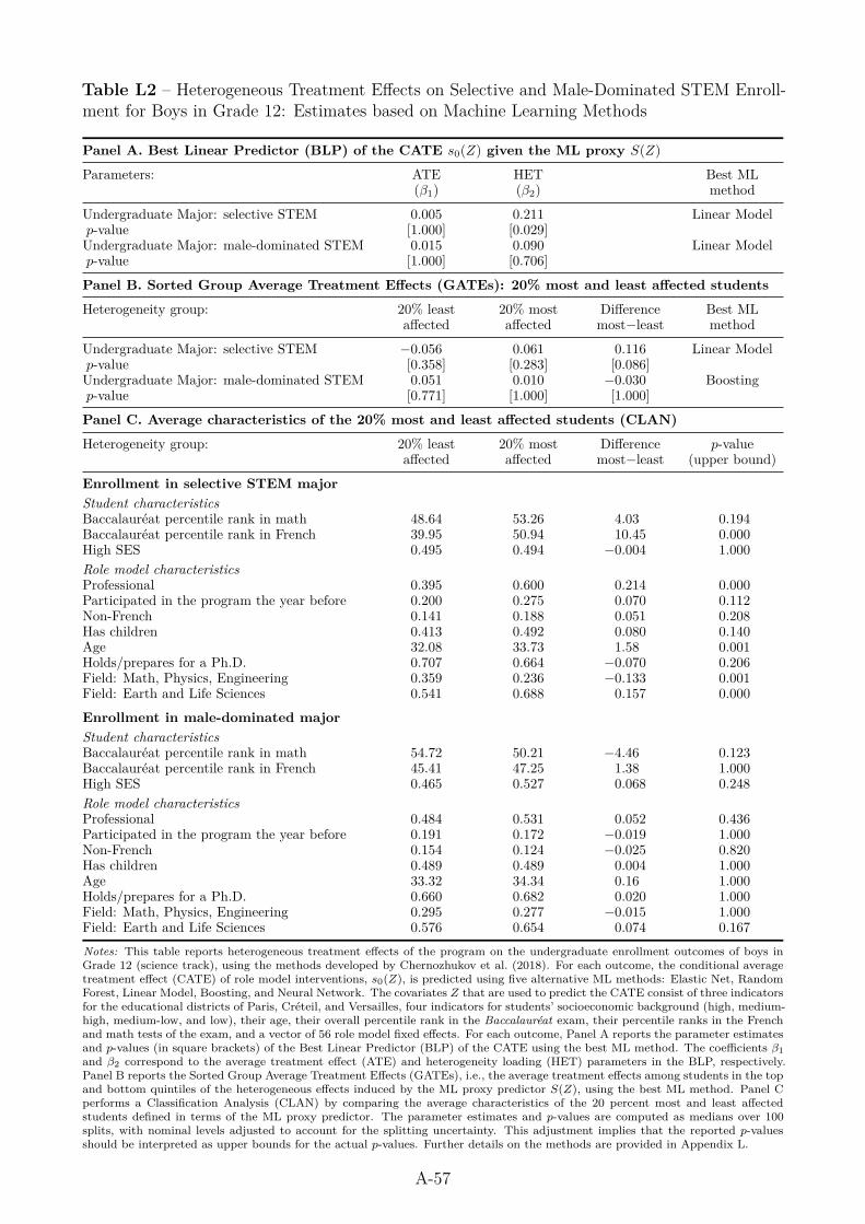
Table L2 – Heterogeneous Treatment Effects on Selective and Male-Dominated STEM Enroll-ment for Boys in Grade 12: Estimates based on Machine Learning Methods

Panel A. Best Linear Predictor (BLP) of the CATE s0(Z) given the ML proxy S(Z)

Parameters: ATE HET Best ML(β1) (β2) method

Undergraduate Major: selective STEM 0.005 0.211 Linear Modelp-value [1.000] [0.029]Undergraduate Major: male-dominated STEM 0.015 0.090 Linear Modelp-value [1.000] [0.706]

Panel B. Sorted Group Average Treatment Effects (GATEs): 20% most and least affected students

Heterogeneity group: 20% least 20% most Difference Best MLaffected affected most−least method

Undergraduate Major: selective STEM −0.056 0.061 0.116 Linear Modelp-value [0.358] [0.283] [0.086]Undergraduate Major: male-dominated STEM 0.051 0.010 −0.030 Boostingp-value [0.771] [1.000] [1.000]

Panel C. Average characteristics of the 20% most and least affected students (CLAN)

Heterogeneity group: 20% least 20% most Difference p-valueaffected affected most−least (upper bound)

Enrollment in selective STEM majorStudent characteristicsBaccalauréat percentile rank in math 48.64 53.26 4.03 0.194Baccalauréat percentile rank in French 39.95 50.94 10.45 0.000High SES 0.495 0.494 −0.004 1.000Role model characteristicsProfessional 0.395 0.600 0.214 0.000Participated in the program the year before 0.200 0.275 0.070 0.112Non-French 0.141 0.188 0.051 0.208Has children 0.413 0.492 0.080 0.140Age 32.08 33.73 1.58 0.001Holds/prepares for a Ph.D. 0.707 0.664 −0.070 0.206Field: Math, Physics, Engineering 0.359 0.236 −0.133 0.001Field: Earth and Life Sciences 0.541 0.688 0.157 0.000

Enrollment in male-dominated majorStudent characteristicsBaccalauréat percentile rank in math 54.72 50.21 −4.46 0.123Baccalauréat percentile rank in French 45.41 47.25 1.38 1.000High SES 0.465 0.527 0.068 0.248Role model characteristicsProfessional 0.484 0.531 0.052 0.436Participated in the program the year before 0.191 0.172 −0.019 1.000Non-French 0.154 0.124 −0.025 0.820Has children 0.489 0.489 0.004 1.000Age 33.32 34.34 0.16 1.000Holds/prepares for a Ph.D. 0.660 0.682 0.020 1.000Field: Math, Physics, Engineering 0.295 0.277 −0.015 1.000Field: Earth and Life Sciences 0.576 0.654 0.074 0.167Notes: This table reports heterogeneous treatment effects of the program on the undergraduate enrollment outcomes of boys inGrade 12 (science track), using the methods developed by Chernozhukov et al. (2018). For each outcome, the conditional averagetreatment effect (CATE) of role model interventions, s0(Z), is predicted using five alternative ML methods: Elastic Net, RandomForest, Linear Model, Boosting, and Neural Network. The covariates Z that are used to predict the CATE consist of three indicatorsfor the educational districts of Paris, Créteil, and Versailles, four indicators for students’ socioeconomic background (high, medium-high, medium-low, and low), their age, their overall percentile rank in the Baccalauréat exam, their percentile ranks in the Frenchand math tests of the exam, and a vector of 56 role model fixed effects. For each outcome, Panel A reports the parameter estimatesand p-values (in square brackets) of the Best Linear Predictor (BLP) of the CATE using the best ML method. The coefficients β1and β2 correspond to the average treatment effect (ATE) and heterogeneity loading (HET) parameters in the BLP, respectively.Panel B reports the Sorted Group Average Treatment Effects (GATEs), i.e., the average treatment effects among students in the topand bottom quintiles of the heterogeneous effects induced by the ML proxy predictor S(Z), using the best ML method. Panel Cperforms a Classification Analysis (CLAN) by comparing the average characteristics of the 20 percent most and least affectedstudents defined in terms of the ML proxy predictor. The parameter estimates and p-values are computed as medians over 100splits, with nominal levels adjusted to account for the splitting uncertainty. This adjustment implies that the reported p-valuesshould be interpreted as upper bounds for the actual p-values. Further details on the methods are provided in Appendix L.

A-57

Table L3 – Proportion of Random Data Splits for which the Correlation between ConditionalAverage Treatment Effects (CATEs) can be Computed, Girls in Grade 12

Proportion of data splits such that

ρA,B|Z canbe computed* β

B|B2 > 0 β

A|A2 > 0 β

A|B2 β

B|A2 ≥ 0

(1) (2) (3) (4)

When outcome Y B is enrollment in a selectiveSTEM program and outcome Y A is:

Positive perception of science-related careers (index) 0.80 1.00 0.86 0.90

More men in science-related jobs 0.68 0.99 0.89 0.73

Equal gender aptitude for math (index) 0.35 1.00 0.98 0.36

Women don’t really like science 0.34 0.99 0.84 0.40

Women face discrimination in science-related jobs 0.62 1.00 1.00 0.62

Taste for science subjects (index) 0.81 0.99 0.97 0.83

Math self-concept (index) 0.39 0.99 1.00 0.40

Science-related career aspirations (index) 0.64 0.99 1.00 0.65

Number of data splits 3,000 3,000 3,000 3,000

Notes: This table reports, for the sample of girls in Grade 12 (science track), the proportion of random data splits (out of 3,000) forwhich the correlation between the Conditional Average Treatment Effects (CATEs) on outcomes Y A and Y B could be computed.Outcome Y B is always enrollment in selective STEM, while Y A is the outcome listed in the corresponding row of the table.Conditional on the covariates Z, the CATEs on outcomes Y A and Y B are denoted by sA

0 (Z) and sB0 (Z), respectively, whereas their

ML proxy predictors are denoted by SA(Z) and SB(Z), respectively. For each random split, the correlation coefficient ρA,B|Z isestimated as ρA,B|Z = Sign(βA|B

2 )(βA|B2 β

B|A2 )

12 /(βA|A

2 )12 (βB|B

2 )12 , where βk|l

2 is the estimated heterogeneity loading parameterof the Best Linear Predictor (BLP) of sk

0(Z) based on Sl(Z) (with k, l ∈ {A,B}), using the methods in Chernozhukov et al. (2018).Column 1 indicates the fraction of data splits for which ρA,B|Z could be computed. The next three columns report the fraction ofsample splits for which each of the three conditions to compute ρA,B|Z is met, i.e., βB|B

2 > 0 (column 2), βA|A2 > 0 (column 3),

and βA|B2 β

B|A2 ≥ 0 (column 4). The proportion of random splits such that βB|B

2 > 0 varies slightly across rows because for eachpair of outcomes (Y A,Y B), the sample is restricted to observations with non-missing values for both outcomes (see Appendix L).Table 8 in the main text reports the median and 95 percent confidence interval of ρA,B|Z over the first 100 random data splits forwhich ρA,B|Z can be computed. Details are provided in Section 6.3 of the main text and in Appendix L.

A-58

Table L4 – Correlation between Conditional Average Treatment Effects (CATEs) for Girls inGrade 12: Sensitivity Analysis

Bivariate correlation with the CATE onenrollment in a selective STEM program

(from first 100 valid iterations)

Estimate 95% confidence Proportion of(ρA,B|Z) interval valid iterations

Panel A. Data splits such that βA|A2 > 0.1, βB|B

2 > 0.1 and βA|B2 β

B|A2 ≥ 0

Conditional average treatment effect (CATE) on:

Positive perception of science-related careers (index) 0.96 [ 0.21, 5.39] 0.73

More men in science-related jobs −0.68 [−3.33,−0.03] 0.65

Equal gender aptitude for math (index) 0.08 [−1.90, 2.11] 0.33

Women don’t really like science 0.26 [−0.64, 3.75] 0.19

Women face discrimination in science-related jobs −0.31 [−2.20, 0.61] 0.61

Taste for science subjects (index) 0.69 [ 0.07, 3.42] 0.66

Math self-concept (index) −0.06 [−1.85, 1.37] 0.38

Science-related career aspirations (index) 0.34 [−0.61, 1.95] 0.62

Panel B. Data splits such that βA|A2 > 0.2, βB|B

2 > 0.2 and βA|B2 β

B|A2 ≥ 0

Conditional average treatment effect (CATE) on:

Positive perception of science-related careers (index) 0.93 [ 0.21, 5.07] 0.64

More men in science-related jobs −0.68 [−3.26,−0.03] 0.65

Equal gender aptitude for math (index) 0.05 [−1.98, 1.90] 0.31

Women don’t really like science 0.31 [−0.51, 3.44] 0.05

Women face discrimination in science-related jobs −0.30 [−2.12, 0.64] 0.58

Taste for science subjects (index) 0.59 [ 0.07, 2.61] 0.34

Math self-concept (index) 0.05 [−1.68, 1.51] 0.29

Science-related career aspirations (index) 0.31 [−0.64, 1.79] 0.46

Notes: Similarly to Table 8 in the main text, this table reports, for girls in Grade 12 (science track), the estimates of the bivariatecorrelation ρA,B|Z between the Conditional Average Treatment Effect (CATE) on enrollment in a selective STEM program, denotedby sB

0 (Z), and the CATE on each of the potential channels listed in the table, denoted by sA0 (Z). The difference is that estimates

provided in this table are obtained using only iterations of the data-splitting process for which the estimates of the heterogeneityloading parameters βA|A

2 and βB|B2 are above a certain threshold. This threshold is set at 0.1 in Panel A and at 0.2 in Panel B.

These restrictions are applied to check the sensitivity of the correlation estimates to excluding data splits that yield a poor MLprediction of the CATEs on outcomes Y A or Y B . Column 3 indicates the proportion of data splits satisfying the restrictionsspecified in each panel’s heading. The estimates and 95 percent confidence intervals reported in columns 1 and 2 are obtained usingthe first 100 data splits satisfying these restrictions. Additional details are provided in the notes of Table 8 and in Appendix L.

A-59

Appendix ReferencesAnderson, Michael L., “Multiple Inference and Gender Differences in the Effects of EarlyIntervention: A Reevaluation of the Abecedarian, Perry Preschool, and Early TrainingProjects,” Journal of the American Statistical Association, 2008, 103 (484).

Athey, Susan and Guido W. Imbens, “The Econometrics of Randomized Experiments,” inEsther Duflo and Abhijit V. Banerjee, eds., Handbook of Economic Field Experiments, Vol. 1,Elsevier, 2017, pp. 73–140.

Beede, David, Tiffany Julian, David Langdon, George McKittrick, Beethika Khan,and Mark Doms, “Women in STEM: A Gender Gap to Innovation,” 2011. U.S. Departmentof Commerce, Economics and Statistics Administration, Issue Brief No. 04-11.

Benjamini, Yoav, Abba M. Krieger, and Daniel Yekutieli, “Adaptive Linear Step-upProcedures that Control the False Discovery Rate,” Biometrika, 2006, 93 (3), 491–507.

Chernozhukov, Victor, Mert Demirer, Esther Duflo, and Iván Fernández-Val,“Generic Machine Learning Inference on Heterogenous Treatment Effects in RandomizedExperiments,” 2018. NBER Working Paper No. 24678.

Davison, Anthony C. and David V. Hinkley, Bootstrap Methods and their Application,Cambridge University Press, 1997.

Duflo, Esther and Emmanuel Saez, “The Role of Information and Social Interactions inRetirement Plan Decisions: Evidence from a Randomized Experiment,” The Quarterly Journalof Economics, 2003, 118 (3), 815–842.

Fisher, Ronald A., The Design of Experiments, McMillan, 1935.Gayral-Taminh, Martine, Tomohiro Matsuda, Sylvie Bourdet-Loubère, ValérieLauwers-Cances, Jean-Philippe Raynaud, and Hélène Grandjean, “Auto-évaluationde la qualité de vie d’enfants de 6 à 12 ans : construction et premières étapes de validationdu KidIQol, outil générique présenté sur ordinateur,” Santé Publique, 2005, 17 (2), 167–177.

Imbens, Guido W. and Donald B. Rubin, Causal Inference in Statistics, Social, andBiomedical Sciences, Cambridge University Press, 2015.

Kuhn, Max, “Building Predictive Models in R using the caret Package,” Journal of StatisticalSoftware, 2008, 28 (5), 1–26.

McDonald, Judith A. and Robert J. Thornton, “Do New Male and Female CollegeGraduates Receive Unequal Pay?,” Journal of Human Resources, 2007, 42 (1), 32–48.

Paz, Lourenço S. and James E. West, “Should We Trust Clustered Standard Errors? AComparison with Randomization-Based Methods,” 2019. NBER Working Paper No. 25926.

Rosenbaum, Paul R., Observational Studies, Springer, 2002., Design of Observational Studies, Springer Series in Statistics, 2010.

Vazquez-Bare, Gonzalo, “Identification and Estimation of Spillover Effects in RandomizedExperiments,” 2018. Manuscript.

Wager, Stefan and Susan Athey, “Estimation and Inference of Heterogeneous TreatmentEffects using Random Forests,” Journal of the American Statistical Association, 2018, 113(523), 1228–1242.

A-60