do babysitters have more kids? the effects of teenage work ...ftp.iza.org/dp6856.pdf iza discussion...
TRANSCRIPT

DI
SC
US
SI
ON
P
AP
ER
S
ER
IE
S
Forschungsinstitut zur Zukunft der ArbeitInstitute for the Study of Labor
Do Babysitters Have More Kids? The Effects of Teenage Work Experiences on Adult Outcomes
IZA DP No. 6856
September 2012
Zeynep ErdoganJoyce JacobsenPeter Kooreman
Do Babysitters Have More Kids? The Effects of Teenage Work Experiences
on Adult Outcomes
Zeynep Erdogan Tilburg University
Joyce Jacobsen
Wesleyan University
Peter Kooreman Tilburg University
and IZA
Discussion Paper No. 6856 September 2012
IZA
P.O. Box 7240 53072 Bonn
Germany
Phone: +49-228-3894-0 Fax: +49-228-3894-180
E-mail: [email protected]
Any opinions expressed here are those of the author(s) and not those of IZA. Research published in this series may include views on policy, but the institute itself takes no institutional policy positions. The IZA research network is committed to the IZA Guiding Principles of Research Integrity. The Institute for the Study of Labor (IZA) in Bonn is a local and virtual international research center and a place of communication between science, politics and business. IZA is an independent nonprofit organization supported by Deutsche Post Foundation. The center is associated with the University of Bonn and offers a stimulating research environment through its international network, workshops and conferences, data service, project support, research visits and doctoral program. IZA engages in (i) original and internationally competitive research in all fields of labor economics, (ii) development of policy concepts, and (iii) dissemination of research results and concepts to the interested public. IZA Discussion Papers often represent preliminary work and are circulated to encourage discussion. Citation of such a paper should account for its provisional character. A revised version may be available directly from the author.
IZA Discussion Paper No. 6856 September 2012
ABSTRACT
Do Babysitters Have More Kids? The Effects of Teenage Work Experiences on Adult Outcomes*
We examine the work experiences during middle school and high school of U.S. females and males and find that most of the child-oriented work such as babysitting and camp counseling is done by females. If the type of work undertaken while young affects either development of specific human capital or preferences, then these early work experiences may have measurable effects on later life outcomes. This paper examines whether or not having a job as a teenager, and whether or not it is a child-oriented job, causes differences in labor market behavior among young adults. In addition to a set of standard controls, in order to account for the endogeneity of students’ work decisions, we utilize a set of state-level instruments, including state-level child-labor laws and indicators of relative demand for, and supply of, child-oriented workers. While the effects we find are complex and sometimes hard to interpret, they suggest that work in 10th grade has a positive causal effect on later labor market outcomes and delays family formation, but to a lesser extent when jobs were child-oriented. JEL Classification: J13, J24 Keywords: human capital, gender, jobs while in school, labor market, family formation Corresponding author: Joyce Jacobsen Department of Economics Wesleyan University PAC 123 238 Church Street Middletown, CT 06459-0007 USA E-mail: [email protected]
* Thanks to Ali Chaudhry for outstanding research assistance. We use the restricted version of the National Educational Longitudinal Study of 1988; thanks to the Institute of Education Sciences Data Security Office Staff for very timely turnaround on all security clearance matters related to our use of these data.

1
I. Introduction
There are a number of reasons why one would expect both job-holding in general and
child-oriented job holding in particular to have effects on future career and life outcomes. The
human capital accumulated in part-time work undertaken while still in secondary school may
provide young people with certain skills which might be critical in determining future career
choices and outcomes. As with schooling, there are many ways in which working during high
school can be beneficial to one’s future career. Familiarizing oneself with business life in general
such as taking responsibility and learning to work together with colleagues could be an important
advantage in starting one’s full-time work career. The experience of looking for a job may in
itself help workers in finding jobs after they leave school. Also, working while studying may
provide students with a social network which may be useful in finding future jobs.
But not all teenager jobs may be the same in terms of acting as a bridge to well-paying
professions. In addition, there are differences in the types of jobs that different groups of high
school students undertake. The benefits of child-oriented jobs might not be the same as other
teenager jobs since the experience acquired via child-oriented jobs in school might not help them
in future job market and might lead them to housekeeping in the future. For instance, when the
high school work experience of females and males is examined, as in Kooreman (2009), it
appears that most of the babysitting is done by females. If work experience early in life teaches
and reinforces traits such as being caring, patient and soft for females and being responsible, on
time and tough for males; this might lead to differential job and career choices between sexes.
That is, if babysitting triggers early parenthood and reduced career prospects because it does
provide experience in handling children, but not how to handle office work, then human capital
2
acquired by doing babysitting might be the reason why females are less participating in labor
force.
In addition, working while attending secondary school may either enhance or detract
from one’s subsequent academic attainment. On the one hand, working while in school might
detract from time and effort dedicated to enhancing academic achievement. On the other hand,
some jobs may have a positive effect on educational attainment since increased involvement in
the job market in one way or another might increase awareness about the importance of
education in school. Another avenue for effects on later behavior may be through modifying
one’s preferences for having children and for particular types of activities. For example,
substantial exposure to child care while young might either make a person more likely to want to
start a family of one’s own, or less likely. Since child-oriented job holders are dealing with
children as a job, their accumulation of child-raising-related human capital might play a positive
role for their fertility decisions. At the same time, there might be a change in their preferences
about having children, either positive or negative. Meanwhile, those who do other jobs might be
expected to have fewer, later children because their accumulated human capital may increase
their labor force participation in the future, which tends to delay and/or reduce childbearing, and
they do not have as much exposure to children, and thus less changes in their preferences
regarding having children (which again could be positive or negative). This could thus lead to
very different decisions regarding educational attainment, timing of marriage and childbearing,
and employment participation. Thus both preferences and constraints (i.e., investments in
specific human capital) may be affected by early work experiences.
This paper looks at the effects of working as a teenager in child-oriented jobs such as
babysitting and camp counseling, both as measured against holding a job in general and as
3
compared to not working during high school. The possible contribution of this pattern to the
overall gender difference in economic outcomes makes these jobs of particular interest. We
consider whether participation in these type of jobs causes differences in young adulthood in
educational attainment, childbearing, participation in paid work, type of occupation, and earnings
rate.
An obvious problem is that participation in work, let alone child-oriented work, during
high school may be caused by the same underlying factors that lead one to make particular
choices as a young adult. In order to account for the endogeneity of both choosing to work and
child-oriented job choice (i.e., the unobserved heterogeneity in the sample), this study uses
several sources of exogenous variation of demand for teenage labor in general and for child-
oriented jobs by U.S. state. Implicitly we are assuming that teenagers and their parents are not
making their location decisions based on variation in these factors, and thus they can be viewed
as both exogenous to future outcomes and correlated with the likelihood of participating in
teenage work. We show both instrumented and non-instrumented estimates for our various
outcome variables.
In the literature, the relationship between high-school employment and future
employment probabilities and wage rates has received some attention. In the early studies by
Meyer and Wise (1983), D’Amico (1984), and Marsch (1991), high-school employment is
associated with future job holding and increased earnings. The effect of employment in school
on academic performance has also been studied. Greenberger and Steinberg (1980), Mortimer
and Finch (1986), Barone (1993), and Steinberg et al (1993) find that high school employment is
associated with lower grade point averages, the further implication being that lower grade point
averages lead to less favorable employment outcomes later in life. Conversely, both Meyer and

4
Wise (1982) and Lillydahl (1990) detect either no effects or beneficial impacts at low or
intermediate work hours.
One of the pitfalls plaguing the early research is the inability of the researchers to control
for the nonrandomness of the student decision as to whether or not to work, which is potentially
affected by factors which may also play a role in future educational attainment or economic
achievement. This potential endogeneity is treated in the works of Ruhm (1997), Hotz et al
(2002), and Tyler (2003). Although Ruhm (1997) finds a positive effect of employment in school
on employment hours and earnings, Hotz et al (2002) find no evidence that employment in
school brings higher future wages. Tyler (2003) reports negative effects of employment in school
on grade point average, but Buscha et al (2008) find no effect of working during the 12th grade
on reading and math scores.
This paper contributes to the literature in several ways. Firstly, to the authors’ knowledge,
none of the previous studies investigates whether doing a certain job while at school, such as
babysitting, has a measurable effect relative to other jobs (and relative to not working).
Secondly, we consider a wider, and different, range of outcome variables relative to the more
recent studies, including both social and economic outcomes. While both Tyler (2003) and
Buscha et al (2008) use the same data set as we do, they concentrate on educational achievement
while we concentrate on longer-run outcome variables. While we use some of the same
instruments as does Tyler (namely some of the same coding of variations in child labor laws
across states), we expand the set of instruments to include measures of relative demand for child
care (female labor force participation rates, the fraction of young children in the state’s
population) and potential supply of teenage workers (fraction of teenagers in the state’s
population). Babysitting is also of interest because of its relatively informal nature, implying that

5
it may be a popular work option both for teenagers too young to work in the formal sector, and
for older teenagers in states where teenagers’ access to the formal sector is more constrained.
Thirdly, we consider how these differences in teenage work patterns by gender could contribute
to different outcomes by gender among young adults.
The rest of this study is structured as follows. Section II presents the data and some
descriptive statistics. Section III explores the selected variables for the regression equation on
their theoretical relevance and discusses estimation methodology. Section IV compiles the
findings. Section V discusses the implications of the findings.
II. Data and Some Descriptive Statistics
The data used in this study are from the National Education Longitudinal Study of 1988
(NELS 88), from the initial data collection through the fourth follow-up survey. These data allow
us to examine young workers as they enter the labor force since it has a detailed work history
from the 8th grade onward. In addition to that, we know as of 2000 (when they are generally 25-
26 years old) their post-secondary schooling, their number of children, their earnings for 2000,
and detailed background characteristics like their family income, and parent’s educational
background. In this dataset, the subjects are first surveyed in the spring of 1988 when they are
generally 13-14 years old. The survey continues through four follow-ups conducted in 1990,
1992, 1994, and 2000. During the first two follow-ups, the initial respondents were 10th and 12th
graders respectively. Additional subjects are added to the survey in later waves to compensate
6
for nonrespondents. At the time of the 4th follow-up in 2000, the number of observations is
12,140.1
Table 1 shows the types of jobs held by students while attending school. The 12th grade
job type variable is not fully comparable with those of the 8th grade and 10th grade because the
12th grade work variable records only 12th grade work experience, whereas the 8th and 10th
grade work variables ask for the most recent work experience. The exact phrasings of these
questions are shown in appendix table A.1. The majority of students, both male and female,
report working at each survey point. Interestingly, young children actually report higher rates of
working than older children. However, the types of jobs held change greatly over this period,
indicating a replacement of informal work by more formal employment. Almost three-quarters of
female children who work report doing babysitting as 8th grades; this proportion drops
significantly already by 10th grade to about one in five working females, and down to about one
in twelve by 12th grade. About one in twelve male children who work report babysitting in 8th
grade, but fewer than one percent of the working males by 12th grade. Meanwhile other jobs
become important, such as food service and retail clerking for both females and males. For the
purposes of this paper, we define child-oriented jobs as babysitting plus camp counseling.
In Table 2, we consider whether there are differences in control variables besides gender
between the samples. The first column displays averages for all respondents to NELS88 while
the next three columns are for respondents who did child-oriented jobs in 8th, 10th and 12th
grade respectively, and the last three columns are for respondents who did other types of jobs.
1 U.S. Department of Education regulations on use of restricted data require us to round all sample sizes to the nearest multiple of 10. This occurs in all tables in this paper that report number of observations.
7
These means indicate that there are observable differences between students who work in
child-oriented jobs and other students in all grades. In particular, females and whites are more
likely to be occupied with child-oriented jobs. Those holding child-oriented jobs are also more
likely to be slightly older than the full sample, as shown by their greater likelihood of being over
26 in their adult sample.
Amount of Job Holding and Child-Oriented Jobs at School
The primary explanatory variables of interest for our analysis are child-oriented job
holding and other types of job holding during the respondent’s 8th, 10th and 12th grade. Table 3
gives summary statistics on school-year employment for the sample, overall and by gender. It
provides descriptive information on three important dimensions of employment in various grades
for child-oriented job holders and other type of job holders while at school: work status, intensity
of work and wage earned (no wage information is available for the 8th grade). 34% and 45% of
8th graders did child-oriented jobs and other type of jobs for pay respectively in 1988. The
percentage of students who did child-oriented jobs for pay among 10th graders dropped down to
7%. In 1992, about 4% of 12th graders report holding a child-oriented job. Thus the proportion
of students who hold child-oriented jobs declines significantly as students move to higher grades.
One possible explanation for this phenomenon is that more alternative job opportunities
become available for the students as they move to upper grades. It is also plausible that the
number of students doing child-oriented jobs is underreported because the students are asked to
report only their job that pays the most per hour. Thus, if students do multiple jobs then they are
less likely to report child-oriented jobs as they tend to pay less: this is supported by the relevant

8
wage comparison in Table 3, where the difference in pay between child-oriented jobs and other
types of jobs is statistically significant.
While a continuous “hours of work” variable would have been preferred, due to data
unavailability, hours of work is calculated from a categorical variable. Hours per week in this
variable are shown as falling into one of five 10-hour interval categories for the 8 th and 10 th
grades, and nine 5-hour interval categories for the 12 th grade, where we take the midpoint of the
category as the relevant value. Those employed in child-oriented jobs in the 8th, 10th, and 12th
grades work on average 5, 16 and 13 hours per week respectively, while those holding other
types of jobs work on average 6, 18, and 18 hours per week respectively. While the mean hours
worked in the 10th grade is greater than the mean hours worked in the 12th grade, this
comparison may be biased because of the difference in the categorization of the hours
variable.Note, however, that this does not affect the within-year comparisons between of hours
worked by students in child-oriented jobs and in other jobs, and comparisons between genders.
These differencesare statistically significant for the three grades.
Regarding differences in work experience by gender, females are more likely to work in
child-oriented job types while males are more likely to work in other type of jobs. Males who are
holding other types of jobs work longer hours on average than females who are holding other
types of jobs. This difference in hours worked is statistically significant for all three grades.
Moreover, in both 10th and 12th grade, the difference in the number of hours worked between
male and females doing child-oriented jobs is statistically significant, with men working more
hours. All gender differences in the table are statistically significant at the 5% level or greater,
save for the weekly hours of work for 8th graders holding child-oriented jobs.
9
The average wages per hour illustrate that females earn less on average than their male
counterparts for both the 10th and 12th grades regardless of job type. In addtion, since they are
more likely to hold child-oriented jobs, which pay less on average and involve fewer hours of
work per week, they earn even less overall. These differences are statistically significant for both
grades and all jobs.
School-year Job Holding, Child-Oriented Jobs, and Future Outcomes
In this paper, we measure the effect of school-year employment and specifically child-
oriented job holding on career prospects by its impact on respondent’s educational attainment,
marital status, number of children, employment status, occupational category, and annual
earnings, all measured as of 2000.2 These variables all indicate important life steps and career-
related activities where it would be interesting to see if they are affected by actions taken while
in secondary school. While the dataset contains several post-secondary educational attainment
variables such as associate’s degree, certificates and licenses, we use attainment of the bachelor
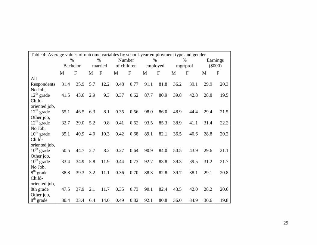
degree or higher as our indicator for educational attainment. Table 4 provides an overview of the
relationship between the type of employment in school and future life outcomes by gender.
There tend to be substantial gender differences for the various outcomes, leading us to
control for gender and for the interaction of gender with job-holding in our subsequent
regressions. Overall, females are more likely to hold a bachelor degree than are males, are more
likely to be married, have more children, are less likely to be employed, more likely to be
managers or professionals, and have lower earnings than do males.
2 In other regressions not reported herein we also consider the impact of school-year employment on the number of hours worked, and the probability of having at least one child. These measures are not reported herein to simplify the exposition; the directionality is similar to that in our reported regressions regarding employment, earnings, and number of children.

10
In comparing child-oriented job holders to other job holders and nonworkers, those
persons holding child-oriented jobs appear to be more likely to hold a Bachelors' degree, less
likely to be married if female (but more likely if male and had such a job in 12th grade), have
slightly fewer children, be somewhat more likely to be employed and more likely to hold a
managerial or professional position. Earnings patterns are less obvious, but appear to show an
intermediate outcome for those holding child-oriented jobs between those holding other jobs and
those holding no mob (in 10th and 12th grade). The question is whether these patterns will hold
up and be of statistical significance once multiple controls are included and some attempt made
to control for endogeneity bias. For that we turn to regression estimation in the next section.
III. Variable Selection and Model Estimation
We have now established the empirical possibility of differential outcomes between
nonworkers, child-oriented job holders and other job holders for the 8th, 10th and 12th grades.
However, we have not controlled for other individually varying factors other than gender in the
descriptive tables. A fuller analysis of the marginal effect of working during school requires us to
control for additional individual covariates and to deal with unobserved heterogeneity that may
be correlated with both outcomes and school-year work choices.
We estimate six sets of regression models, using bachelor degree attainment, marital
status, number of children, employment, managerial/professional occupation, and log of hourly
earnings respectively as dependent variables that capture different life and career outcomes. The
regression equations which will be elaborated upon and estimated in the following sections can
be summarized as the following:

11
(1) Degree Attainment DT = D(XDT, XDS, COs, Es)
(2) Marriage MT = M(XMT, XMS, COs, Es)
(3) Number of Children NT = N(XNT, XNS, COs, Es)
(4) Employment ET = E(XET, XES, COS, Es)
(5) Wage/Earnings WT = W(XWT, XWS, COs, Es)
(6) Occupation OT = O(XOT, XOS, COs, Es)
where the subscript T indicates the value as of 2000 and the subscript S indicates the value as of
the earlier year of schooling (whether 8th, 10th, or 12th grade).
One critical issue in estimating the impact of child-oriented jobs in school on outcomes is
the issue regarding self-selection of students into job type in school. In other words, if certain
student characteristics such as coming from privileged families are directly related to job type at
school and future career and life choices, then any difference observed between child-oriented
job holders and other type of job holders may be due to these preexisting differences. The effects
of child-oriented jobs and employment while in school on future choices could only be
demonstrated by controlling for the characteristics potentially influencing both employment
choice in school and future outcomes. In order to control for pre-existing differences between
students, extensive sets of covariates are included in the regression models (X.S). Others of these
covariates relate to the person’s current location, such as their current geographical location and
current family status (X.T). The supplementary covariates X that are found in all six models
include standard demographic variables indicating female, race and ethnicity (white, black and
hispanic vs. the omitted category of all other racial and ethnic groups), geographic region
(northeast, south, and north central vs. the omitted category of west), residence in an urban or

12
suburban area (vs. the omitted category of rural area), whether the respondent has limited
English capacity, income other than employment and partner’s income (these categories are
either time-invariant or relate to the adult time period).
Each model contains a dummy COs for child-oriented job and a dummy Es for holding
any type of job while in school at time S (where S precedes T). This allows us to consider how
working during school years affects outcomes and see if the particular category of job, namely
child-oriented, modifies this effect at all. These dummy variables are also interacted with the
dummy variable for female. This allows us to see if the effect of working varies by gender, as
well as whether the effect of working in a child-oriented jobs varies by gender. We estimate
three different variants of each model, where CO and E can be related to 8th grade, 10th grade,
or 12th grade job holding. This allows us to see whether work at different points during one's
schooling career affects outcomes differently. We choose not to include 8th, 10th, and 12th grade
job holding simultaneously. This would complicate the interpretation of the results since work in
later grades might be affected by work in previous grades.
With regard to estimation of model (1), one issue is that students who have relatively less
unobserved ability for educational achievement may be more inclined to participate in work
while in school. Therefore, a measure of 8th grade educational achievement (as calculated by the
NELS) is included as a control. Also, students whose parents have lower incomes are expected to
work more while studying. If that is left uncontrolled, then the sample is no longer random.
Therefore, the family background variables (as of the 8th grade) of family income, mother’s
education, and father’s education are included in the model as controls. We also include type of
school attended in the 10th grade (private nonreligious and public vs. the omitted category of
private religious). In addition, we control for the number of siblings, and whether the

13
respondent’s family in 8th grade had an encyclopedia, atlas, dictionary and computer in the
home.
The number of children one has is expected to be related to human capital acquired which
pertains to raising children or due to a change in preferences. The additional covariates of
whether or not the person has a sibling and birthyear are also included in model (3), as slightly
older persons in this age range are more likely to have children, and the presence or absence of a
sibling may affect childbearing preferences.
In model (5), the control variable vector XW includes a more detailed set of educational
attainment indicators (high school degree, some post-secondary study, certificate, associate
degree, bachelor’s degree, master’s degree, and professional degree relative to non-completion of
the high school degree), and years of experience (and experience squared) in paid work,
variables demonstrated to affect earnings in many other earnings studies.
In model (6), the control variable vector XW includes the same more detailed set of
educational attainment indicators as in model (5), as educational attainment appears relevant for
occupation.
Because of the discrete nature of bachelor degree attainment, marital status, employment
status, and managerial/professional occupation holding, a probit model is used for estimation of
models (1), (2), (4), and (6). For number of children, because 62 percent of the sample does not
have any children, model (3) is estimated using tobit. To estimate model (5), as is conventional
in the literature, the natural logarithm of annual earnings rather than its level is used as the
dependent variable. In addition, for model (6), because earnings are not observed for people who
are not working, the two-step Heckman selection model (Heckit) is used for estimation. The
earnings equation has experience and its squared value, which is not included in the selection
14
step, whereas the selection equation has income other than employment, partner’s income, and
the number of children, all of which are not included in the earnings equation.3
Although controls are included in all six models, it is important to note that one has to be
careful with using direct methods for measuring the effect of school-year work, since unobserved
heterogeneity left in the error term, even after additional controls are added in the models, could
lead to biased estimates of the effect of holding child-oriented jobs and jobs in general. Thus
instrumental variable estimation would be preferred so long as reasonable instruments can be
obtained. Thus we consider whether we can identify plausible instruments that would affect
students’ free choice of work during the school year or would provide demand- or supply-shocks
to the teenage labor market.
First, we use a set of state-level child labor law indicators as instruments. These laws
restrict the range of formal job options a student has, both in terms of access to particular jobs, in
limiting the number and timing of hours that one might work or the amount that one might earn
in those jobs For example, an exogenous tightening of child labor laws in a state might mean that
a student could work fewer hours in formal jobs such as retail, and the time would be replaced by
working in lower-paying adolescent jobs in the informal sector such as babysitting and lawn
care.
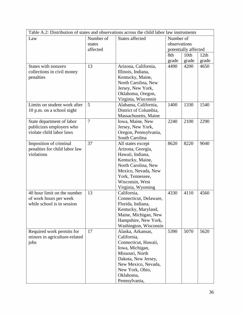
The child labor law instrument set that affects teenager’s job type in different states
contains seven binary variables. The state level data about child labor law variation is taken from
Tyler (2003). These are as follows:
1. The state collected civil monetary penalties;
3 [Note for editor/readers: Full results from the equations not highlighted in the paper may be made available by the authors in an online appendix. Similarly, the current appendix tables may be all or partly moved to an online appendix as the journal sees fit.]

15
2. The state had regulations that placed limits on adolescent work after 10:00 p.m. on a
night before a school day;
3. The state labor department was required to publicize the names of employers who
violate child labor laws;
4. The state imposed criminal penalties for child labor violations;
5. The state limited the maximum number of hours that adolescent minors could work
during a school week;
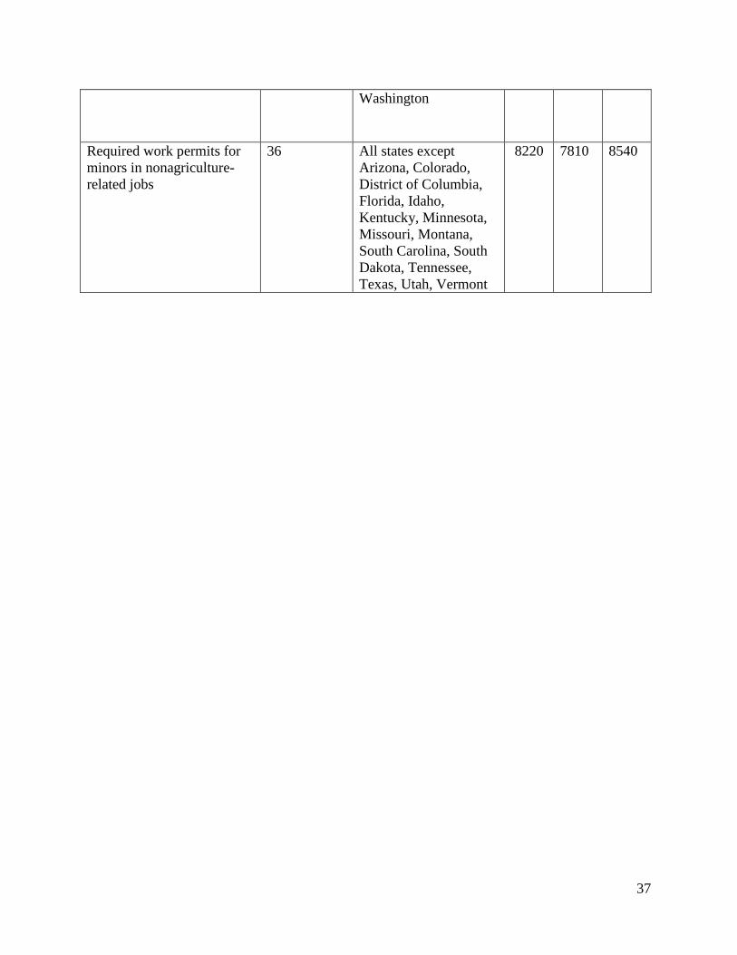
6. The state required work permits for minors employed in agriculture-related jobs;
7. The state required work permits for minors employed in nonagriculture-related jobs.
Appendix table A.2 considers how many observations are potentially affected by each type of
child labor law.
Additional instruments we use are the female labor force participation rate, the 0-11 year
old fraction of the population and the 12-18 year old fraction of the population for each state .
Female labor force participation and the relative size of the 0-11 year old population are
hypothesized to be indicators of demand for child-oriented jobs like babysitting, while 12-18
year old population is hypothesized to be an indicator of relative supply of teenage labor. Thus
we attempt to identify the effects of teenage job holding through the geographic variation in
demand and supply for teenage labor, both of which are arguably exogenous to the individual’s
desire to work. One can argue that babysitting is done in general at night and camp counseling is
done on holidays and therefore female labor force participation might not be that important
factor for determining demand for child-oriented jobs. However, going out at night might also be
correlated with female labor force participation since higher income couples might be more

16
likely to be working. Also, sending the child to a camp might also be correlated with family
income and mother’s free time to deal with the child.
One crucial assumption for identifying the effect of child-oriented jobs and other types of
jobs on future career prospects is that child-labor laws, female labor force participation, 0-11
year old and 12-18 year old population only affect future outcomes via their effects on type of
job in school. This is not testable. The other assumptions are that they are indeed correlated with
the endogenous variables of interest (which is testable).
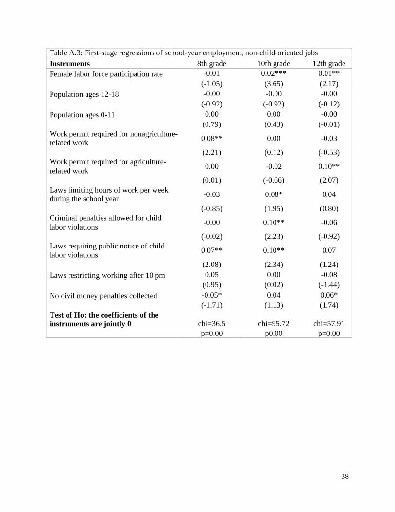
To test that these potential instruments are indeed correlated with the endogenous
explanatory variables of interest, we estimate first-stage regressions where job holding is
regressed on the child labor law instrument set, the female labor force participation rate, the
fraction aged 0-11 in the population, the fraction aged 12-18 in the population and other
exogenous variables. Appendix tables A.3 and A.4 contain the coefficients for these variables for
the first stage regressions for non-child-oriented and child-oriented jobs4 Although some of the
first stage coefficients are counterintuitive5, the hypothesis that the coefficients on the
instruments are jointly zero is rejected at the 1% significance level; therefore, we may conclude
the instruments are related to 8th, 10th and 12th grade choice of job type. Thus the instruments
pass this formal test of relevance. We also conduct Wald tests in the various specifications of
models (1) through (6) which indicate that the two variables of interest, COs and Es, are indeed
best treated as endogenous—implying that in general the IV results are to be favored over the
non-IV results. However, if results are not found in either the non-IV or the IV results, this
4 In the interest of saving space, the coefficients on the other controls are not displayed in the table, but available in our online appendix. 5 For example, in table A4 we expected the coefficients on the fractions of the population aged 12-18 and aged 0-11 to be negative and positive, respectively. Note, however, that state averages might misrepresent local compositions of the population.

17
would be strongly consistent with the null hypothesis view that there is no effect of school-time
employment on future outcomes.
IV. Regression Results
Education
Table 5 presents probit estimates of the main items of interest from model (1), namely the
marginal effect of working while in school, along with the additional effect of whether the
person holds a child-oriented job, of being female, and the interaction of working and holding a
child-oriented job with being female. Partial effects are calculated at the mean values for the
sample. For each set of results, we run equations controlling for child-oriented jobs and job-
holding overall in the 8th, 10th and 12th grades of school. Both non-IV and IV estimates are
included for comparison for each case, leading to a total of six columns in each table. All the
following results tables follow this same format. The full set of coefficients for model (1) is
available in appendix table A.5.
Although in the descriptive information presented in the previous section, child-oriented
job holders were found to be more likely to hold a bachelor degree, once we control for other
covariates, this pattern dissipates for all but 10th grade job-holding in the instrumented results. In
this case, persons who work, particularly in child-oriented jobs, are more likely to receive a
bachelor's degree.
When one compares the noninstrumented and instrumented columns, the estimated effect
of employment in the 12th grade which is negative in the noninstrumented estimates is no longer
negative under IV estimation once endogeneity of working is treated. For instance, employment

18
in 12th grade has statistically a significant negative coefficient. Unobserved heterogeneity in this
case could be that those who work in the 12th grade might be those do not want to go to college
after school ; we might call them potential drop-outs. Once potential drop-outs are accounted for
under IV estimation as shown in the last column, employment in 12th grade compared to non-job
holders does not have a statistically significant effect on bachelor degree attainment. In other
words, it does not seem like working in 12th grade detracts from efforts that should be properly
dedicated to enhanced academic achievement.
The strongest IV effects, in terms of both size and significance of coefficients, are found
for working in 10th grade. For boys working in 10th grade makes it more likely to attain a
bachelor degree several years later (with Average Partial Effect, APE=0.49), in particular if the
job was child-oriented (APE=0.49+0.72). Girls are more likely to attain a bachelor degree
irrespective of school-year work (APE=0.393). Working in 10th grade makes this more likely,
but to a lesser extent than for boys (additional APE of working is 0.49-0.34). The effect is
slightly larger if the job was child-oriented (APE=0.49-0.34+0.72-0.50).
Marital status
Table 6 presents probit estimates of the marginal effects of interest from model (2). The
full set of coefficients for model (2) is available in appendix table A.6. Working in the 8th grade
has a positive effect on marital status. The 10th and 12th grade non-IV estimates have a similar
sized effect of increasing the probability of being married by about three percent. The 12th grade
IV estimates suggest that holding a child-oriented job reduces the probability of being married (-
0.072), in particular for females (-0.072-0.070) On the other hand holding a child-oriented job in
the eighth grade has a substantial positive effect on marital status for females.

19
Fertility
Table 7 presents tobit estimates of the marginal effects of interest from model (3). The
full set of coefficients for model (3) is available in appendix table A.7. Being employed in the
8th grade has a positive effect on childbearing for boys, unless the job was child-oriented. For
girls the effect is negligible. Most of the tenth grade coefficients are insignificant. The twelfth
grade IV results suggest a negative effect of child-oriented jobs on the number of children, but
not for females who worked in a child-oriented job. The size of this coefficient is very large,
casting suspicion on the fit of the IV equation.
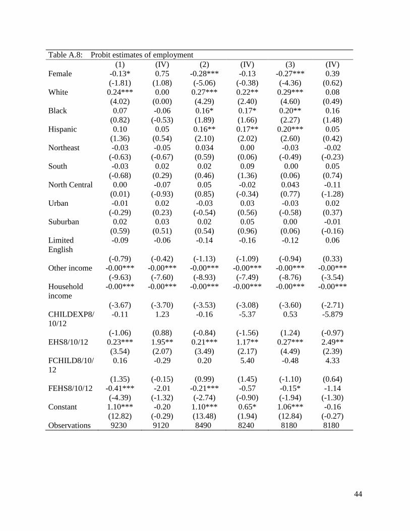
Employment status
Table 8 presents probit estimates of the main coefficients of interest from model (4); the
full set of coefficients for model (4) is available in appendix table A.8. Working has a positive
effect on young adult employment status in all six specifications, and it is much largerin the IV
specifications. However, for women, the effect is reversed in some of the specifications. Having
had a child-oriented job appears to somewhat reduceof the employment probability, according to
the IV specifications for 10th and 12th grade; less so for women than for men in this category.
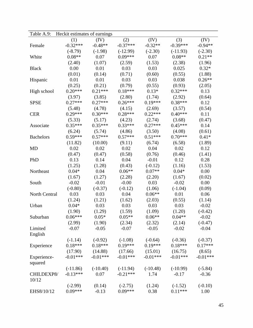
Earnings
Table 9 presents heckit estimates of the main coefficients of interest from equation (6);
the full model is available in appendix table A.9. The coefficient on female in this table captures
the percentage difference in the average wage between women and men holding other factors
constant; as expected, it is significantly negative. The interactions with type of work and gender
20
are complex. Working has a nonnegative effect for men and for women in most of the
regressions, but early (8th grade) work has a negative effect for women in the non-IV regression,
but less so if it is a child-oriented job. For men, working in a child-oriented job in the 8th grade
or 10th grade has a negative effect.
Occupational categories
Given that the child-oriented school-year job holders are found to have an earnings
disadvantage in the future under the noninstrumented estimates but not under IV, and that child-
oriented job holding is not found to be a significant factor for employment status, whether this
pattern is because child-oriented job holders choose to work in certain type of occupations
becomes of additional interest. Thus we analyze the workers’ 2000 occupational distribution in
this section, classifying occupations according to the ILO’s 2008 classification. Table 10
displays the six occupational type categories that we utilize in the following formal analysis and
the associated occupations within each of those categories.
Armed force occupations are discarded due to the small number of observations and
agricultural workers are put into the craft workers category. The craft workers category also
includes plant and machine operators, assemblers and other relatively lower-educational-
attainment requirement occupations. The information on the distribution of main occupational
categories is given inside the parentheses below each category in the first column. For instance,
the managers category accounts for 12.3% of all workers in the sample. In addition, for each
broader occupational category, the percentage distribution of occupations within that category is
given inside the parentheses next to the category title. For example, 29% of managers in our
sample are mid-level managers.
21
We then estimated a probit model in order to predict the probability of an individual’s
being in one of the generally higher-paying, more prestigious occupational categories of either
manager or professional (versus all other categories).6 Table 11 provides the estimated marginal
effects of the main variables of interest (the full coefficient set is in appendix table A.10). There
is little evidence of an effect of any of the variables of interest on occupational category, save for
some effect from working in the 10th grade that apparently makes one more likely to be in a
managerial or professional occupation.
V. Discussion and Conclusions
The importance of evaluating how formative teenage work experiences are on adult
outcomes is substantial. There is significant interest among both policymakers and academics on
school-to-work transitions (witness the recent set of papers in Schoon and Silbereisen 2009). The
general view as we continue into the 21st century is that young people no longer have a lock-step
pattern to follow to becoming a successful adult, and the diversity of paths is leading to a
diversity of outcomes. Thus on the one hand it would be interesting to know how determinate
early work experiences are on later lives, and if they are determinate, to modify the choice set of
teenagers accordingly in ways that lead to more positive outcomes later on, in terms of young
people’s achieving economic self-sufficiency and otherwise. In addition, it is interesting to
consider how differences in early life experiences of girls and boys may contribute to differences
by gender in economic and social outcomes later. On the other hand, it would also be nice to
6 We also estimated a multinomial logit model where individuals were predicted as falling into one of the 6 occupational groups; “manager”, “professional”, “technician”, “clerks”, “service”, “crafts.” Based on this model, the results of which are available upon request from the authors, we determined that little sorting power existed between this more detailed set of groups, but that there were similarities between the manager and professional categories; hence the decision to combine them into one group versus the other six, and use a probit specification instead.
22
know if early work experiences do not lock teenagers into particular future patterns, but that
much is still indeterminate about how their lives will unfold.
Our results, while mixed, are provocative. We see interesting nonlinearities in the
patterns depending on which year of school the student undertook work experiences in, and some
evidence of effects of type of work (and work in and of itself) on measurable outcomes. The
effects also appear to vary significantly by gender. It also appears that our instrumental variable
effects give very different results in some cases from the non-IV estimates. One result that stands
out is that work in 10th grade seems to have a positive causal effect on later labor market
outcome and to delay family formation.
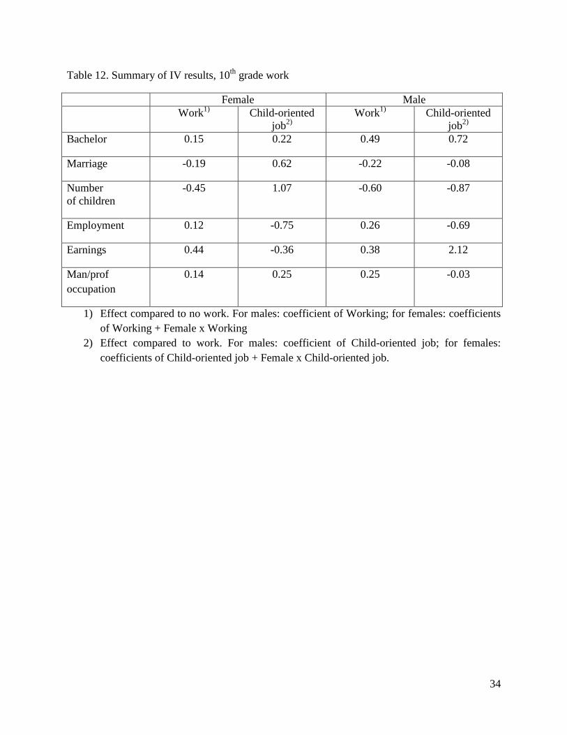
The results presented in the preceding section show a diverse picture of many significant
effects of work while in school on later outcomes. Table 12 provides a different perspective by
summarizing the IV results (which are more likely than the non_IV results to represent causal
effects) for the 10th grade (which generally show the largest number of significant coefficients.)
Table 12 shows that working in 10th grade leads to more positive labor market related outcomes
(bachelor degree, employment, occupation, and earnings) and lower outcomes in terms of family
formation (marriage and number of children), both for males and females. For females the results
suggest that child-oriented jobs lead to higher family formation outcomes.
Certainly exploration of better instrument sets is one avenue for consideration. We also
would have liked to consider how extracurricular activities besides work experience might affect
future outcomes; however this posed an even more difficult instrumenting problem in trying to
ascertain what activities were available at each school, information not available in our data.
Similarly, we do not have full information on household structure, and on chores and other
nonschool activities that compete for students' time use. Time use diary information in a panel

23
setting, something not currently available, would be interesting to examine for a fuller picture of
how time allocation when young affects future outcomes.
24
References
Barone, F. (1993). The Effects of Part-time Employment on Academic Performance. NASSP
Bulletin 77, 67-73.
Buscha, F., Maurel, A., Page, L. Speckeeser, S. (2008). The Effect of High School Employment
on Educational Attainment: A Conditional Difference-in-Differences Approach. Working
Paper.
D’Amico, R. (1984). Does Employment During High School Impair Academic Progress?
Sociology of Education 57, 152-164.
Greenberger, E., Steinberg, L. (1980). Part Time Employment of In-School Youths: A
Preliminary Assesment of Costs and Benefits. In U.V. Employment, A Review of Youth
Employment Problems, Programs, Policies (pp. 1-15). Washington, D.C.: U.S. Department
of Labor, Employment and Training Administration.
Hotz, V.J., Xu, L.C., Tienda, M., Ahituv, A. (2002). Are There Returns to the Wages of Young
Men from Working While in School? Review of Economics and Statistics 84, 221-236.
Kooreman, P. (2009). The Early Inception of Labor Market Gender Differences. Labor
Economics 16, 135-139.
Lillydahl, J. (1990). Academic Achievement and Part Time Employment of High School
Students. Journal of Economic Education 21, 307-316.
Marsch, H. (1991). Employment During High School: Character Building or a Subversion of
Academic Goals. Sociology of Education 64, 172-189.
Meyer, R., Wise, D. (1983). The Effects of the Minimum Wage on the Employment and
Earnings of Youth. Journal of Labor Economics 1, 66-100.
25
Mortimer, J., Finch, M. (1986). The Effects of Part-Time Work on Adolescent Self-Concept and
Achievement. In K. Borman and J. Reisman, Becoming a Worker (pp. 66-89). Norwood,
N.J.: Ablex.
Ruhm, C., 1997. Is high school employment consumption or investment? Journal of Labor
Economics 14, 735-776.
Schoon, I., Silbereisen, R.K. (eds) (2009). Transitions from School to Work: Globalization,
Individualization, and Patterns of Diversity. Cambridge, UK: Cambridge University Press.
Steinberg, L., Fegley, S., Dornbusch, S. (1993). Negative Impact of Part Time Work on
Adolescent Adjustment: Evidence from a Longitudinal Study. Development Psychology 29,
171-180.
Tyler, J.H. (2003). Using state child labor laws to identify the effect of school-year work on High
School Achievement. Journal of Labor Economics 21, 381-408.

26
Table 1: Types of Jobs held while attending school, overall and by gender
8th graders 10th graders 12th graders
All Fem. Male All Fem. Male All Fem. Male Percent working 79.3 77.9 81.0 56.3 51.5 61.8 67.2 68.0 65.6 Type of job if working:
Child-oriented jobs babysitting 42.9 74.1 8.4 11.0 20.9 1.6 4.8 8.4 0.6 camp counselor -- -- -- 2.1 2.1 2.2 0.8 0.7 1.0
Other types of jobs lawn work & odd jobs 23.9 7.6 41.9 6.4 1.3 11.4 2.2 0.2 4.5 newspaper route/ delivery person 6.8 2.6 11.5 2.2 0.6 3.7 1.4 0.3 2.7 farm work 5.6 1.8 9.8 5.0 1.9 8.0 2.1 0.2 4.3 manual labor/ warehouse work 4.7 1.1 8.6 5.3 1.2 9.2 1.7 0.3 3.4 store clerk 2.4 2.1 2.9 11.1 13.8 8.5 27.0 30.6 22.8 food service/ fast food worker 1.6 1.8 1.4 22.2 27.1 17.5 23.2 25.1 20.9 office/clerical 1.2 1.6 0.8 5.2 7.6 2.7 7.5 11.1 3.3 other 10.9 7.3 14.8 25.0 20.9 29.0 24.6 19.2 30.9 house cleaning -- -- -- 1.1 1.7 0.6 0.8 1.0 0.7 hospital/health work -- -- -- 0.8 1.0 0.5 2.0 2.8 1.0 construction work -- -- -- 2.6 0.0 5.2 1.8 0.1 3.9

27
Table 2: Summary statistics for the sample Entire
sample
Child-oriented jobs Other types of jobs
Percent of sample that is/has: 8th grade
10th grade
12th grade
8th grade
10th grade
12th grade
female 52.4 90.7 85.5 86.5 23.8 43.5 47.8 white 68.6 76.6 79.9 85.0 73.2 74.4 76.2 black 9.7 7.7 8.4 4.4 8.6 7.6 6.7 Hispanic 13.4 9.8 7.0 5.9 11.6 10.4 10.4 residing in northeast 19.2 21.1 26.0 24.9 18.5 21.1 21.2 residing in south 33.7 29.1 27.6 31.2 33.4 27.2 25.6 residing in north central 27.2 31.2 28.5 22.0 28.6 32.2 33.9 residing in urban area 25.0 24.6 22.6 21.0 23.0 23.0 22.5 residing in suburban area 43.6 44.6 43.8 51.3 42.5 44.5 45.2 limited English 2.4 1.5 0.4 0.6 2.4 1.8 1.6 at most 1 sibling 38.7 37.5 41.8 42.0 39.2 38.4 40.3 > 26 years old in 2000 65.8 70.9 75.9 79.1 60.4 63.0 66.4 no income other than earnings in 2000 72.5 71.9 70.1 73.0 71.6 71.2 72.1 spouse/partner's income < $10K in 2000 58.5 48.4 49.3 45.3 63.3 58.3 56.5 encyclopedia at home in 8th grade 80.6 81.1 84.0 81.7 81.8 81.7 82.2 atlas at home in 8th grade 70.2 71.2 75.0 74.9 72.9 73.4 73.1 dictionary at home in 8th grade 98.0 98.3 98.8 98.8 97.9 98.5 98.9 computer at home in 8th grade 42.9 41.3 44.1 44.4 45.5 45.0 45.0 mother a high school graduate 36.7 35.7 30.9 33.4 38.7 38.5 39.9 father a high school graduate 35.6 34.1 29.6 33.1 37.8 37.4 38.6 family income < $20K in 1988 26.3 23.8 23.5 19.2 25.7 23.7 22.3 attended public school 82.3 79.4 73.9 76.6 7.5 7.4 6.2 attended private school 7.9 8.8 14.4 13.8 83.3 82.2 82.2 grade average > 3.0 in 1988 57.9 61.3 69.0 65.3 54.3 58.5 61.1 tenure in last job < 1 year 10.4 9.7 9.2 11.5 10.6 10.7 10.2 high school degree 16.0 12.4 12.0 8.5 18.6 16.3 15.1 done some post-secondary education 29.9 28.6 25.1 26.3 30.4 31.0 32.3 some certificate 8.0 8.5 7.3 8.9 7.5 8.1 8.3 Associate's degree 7.3 8.0 8.9 9.5 7.2 7.5 8.8 Bachelor's degree 29.9 33.7 38.8 42.9 28.1 30.4 30.8 Master's degree 3.3 4.6 6.2 3.6 2.4 2.9 3.2 Professional degree 0.6 0.6 0.5 0.3 0.6 0.8 0.6

28
Table 3: Employment during the school year, overall and by gender
8th graders
10th graders
12th graders
All Female Male All
Female Male All
Female Male
Percent having no job
20.7 22.7 19.0 43.7 48.5 38.2 32.8 31.9 34.4
Percent doing child-oriented jobs
34.0 57.7 6.8 7.4 11.8 2.3 3.9 6.2 1.1
Percent doing other types of jobs
45.3 20.2 74.2 48.9 39.7 59.5 63.3 61.9 64.5
Average weekly hours of work, child-oriented jobholders 4.9 4.9 4.5 15.9 15.0 21.4 13.3 12.9 16.2 Average weekly hours of work, other jobholders 6.2 5.9 6.3 17.9 16.7 18.8 17.9 17.3 18.6 Average hourly wage, child-oriented jobholders - - - $3.01 $2.90 $3.68 $4.40 $4.32
$5.58
Average hourly wage, other jobholders - - - $4.40 $4.10 $4.62 $5.33 $5.13
$5.54
29
Table 4: Average values of outcome variables by school-year employment type and gender
%
Bachelor %
married Number
of children %
employed %
mgr/prof Earnings ($000)
M F M F M F M F M F M F All Respondents 31.4 35.9 5.7 12.2 0.48 0.77 91.1 81.8
36.2 39.1 29.9 20.3
No Job, 12th grade 41.5 43.6 2.9 9.3 0.37 0.62 87.7 80.9 39.8 42.8 28.8 19.5 Child-oriented job, 12th grade 55.1 46.5 6.3 8.1 0.35 0.56 98.0 86.0 48.9 44.4 29.4 21.5 Other job, 12th grade 32.7 39.0 5.2 9.8 0.41 0.62 93.5 85.3 38.9 41.1 31.4 22.2 No Job, 10th grade 35.1 40.9 4.0 10.3 0.42 0.68 89.1 82.1 36.5 40.6 28.8 20.2 Child-oriented job, 10th grade 50.5 44.7 2.7 8.2 0.27 0.64 90.9 84.0 50.5 43.9 29.6 21.1 Other job, 10th grade 33.4 34.9 5.8 11.9 0.44 0.73 92.7 83.8 39.3 39.5 31.2 21.7 No Job, 8th grade 38.8 39.3 3.2 11.1 0.36 0.70 88.3 82.8 39.7 38.1 29.1 20.8 Child-oriented job, 8th grade 47.5 37.9 2.1 11.7 0.35 0.73 90.1 82.4 43.5 42.0 28.2 20.6 Other job, 8th grade 30.4 33.4 6.4 14.0 0.49 0.82 92.1 80.8 36.0 34.9 30.6 19.8

30
Table 5: Probit estimates of bachelor degree attainment; average partial effects of child-oriented job and working while in school, and interactions with female 8th 8th-IV 10th 10th-IV 12th 12th-IV Child-oriented job 0.06 -0.11 0.03 0.72*** 0.03 0.25 (1.55) (-0.25) (0.49) (9.81) (0.28) (0.17) Working -0.02 -0.03 0.02 0.49*** -0.06** 0.36 (-0.72) (-0.11) (0.71) (3.26) (-2.56) (0.89) Female Female x Child-oriented job Female x Working
0.09*** (2.86)
-0.04
(-0.99) -0.04
(-1.14)
0.26 (1.22)
-0.06
(-0.09) -0.15
(-0.30)
0.09*** (4.09)
-0.00
(-0.04) -0.06** (-2.10)
0.39*** (3.58)
-0.50*** (-6.39) -0.34* (-1.83)
0.04 (1.52)
0.00
(0.02) 0.04
(1.11)
0.31 (1.41)
-0.09
(-0.05) -0.36
(-1.24)
Observations 6580 6520 6120 5960 5880 5880 t-statistics in parentheses; *** p<0.01, ** p<0.05, * p<0.1 Table 6: Probit estimates of being married; average partial effects of child-oriented job and working while in school, and interactions with female 8th 8th-IV 10th 10th-IV 12th 12th-IV Child-oriented job -0.04** -0.17 -0.04** -0.08 0.03 -0.07** (-2.34) (-1.10) (-2.50) (-1.61) (0.58) (-2.10) Working 0.04*** 0.11** 0.03*** -0.22* 0.03*** -0.32 (4.06) (1.97) (3.70) (-1.71) (4.19) (-0.92) Female Female x Child-oriented job Female x Working
0.08*** (6.18)
0.03
(1.32) -0.02
(-1.59)
0.24* (1.86)
0.83** (2.04) -0.43
(-1.54)
0.06*** (7.40)
0.05
(0.81) -0.01
(-1.33)
0.04 (0.86)
0.71
(0.48) -0.03
(-0.39)
0.06*** (6.21)
-0.02
(-0.91) -0.02** (-2.05)
0.09 (1.21)
-0.07** (-2.11) 0.02
(0.18)
Observations 9580 9460 8800 8530 8460 8460 t-statistics in parentheses *** p<0.01, ** p<0.05, * p<0.1

31
Table 7: Tobit estimates of number of children; average partial effects of child-oriented job and working in school, and interactions with female 8th 8th-IV 10th 10th-IV 12th 12th-IV Child-oriented job -0.10* -1.29*** -0.15** -0.27 0.02 -0.78*** (-1.82) (-2.76) (-2.00) (-0.15) (0.15) (-5.47) Working 0.12*** 1.10*** 0.04 -0.60** 0.07*** -0.89 (3.85) (6.65) (1.41) (-2.05) (2.65) (-1.20) Female Female x Child-oriented job Female x Working
0.24*** (5.93)
0.06
(0.84) -0.01
(-0.14)
1.60*** (4.37)
2.68
(1.47) -1.70** (-2.44)
0.20*** (7.24)
0.16
(1.27) -0.02
(-0.47)
-0.01 (-0.01)
1.34
(0.37) 0.15
(0.44)
0.19*** (6.30)
-0.02
(-0.17) -0.04
(-1.12)
-0.05 (-0.21)
16.59** (2.09) 0.43
(1.01)
Observations 9090 8980 8360 8110 8040 8040 t-statistics in parentheses *** p<0.01, ** p<0.05, * p<0.1 Table 8: Probit estimates of employment; average partial effects of child-oriented job and working while in school, and interactions with female 8th 8th-IV 10th 10th-IV 12th 12th-IV Child-oriented job -0.02 0.21 -0.03 -0.95*** 0.07* -0.93*** (-1.04) (1.14) (-0.79) (-33.92) (1.85) (-31.51) Working 0.05*** 0.60** 0.04*** 0.26** 0.06*** 0.66*** (3.30) (2.15) (3.45) (2.13) (4.27) (2.78) Female Female x Child-oriented job Female x Working
-0.03* (-1.81)
0.03
(1.41) -0.09*** (-4.22)
0.16 (1.13)
-0.07
(-0.16) -0.49
(-1.36)
-0.05*** (-5.12)
0.04
(1.11) -0.04*** (-2.60)
-0.03 (-0.40)
0.20*** (3.18) -0.13
(-0.86)
-0.05*** (-4.40)
-0.12
(-0.90) -0.03* (-1.90)
0.07 (0.65)
0.14*** (3.22) -0.25
(-1.25)
Observations 9230 9120 8490 8240 8180 8180 t-statistics in parentheses *** p<0.01, ** p<0.05, * p<0.1

32
Table 9: Heckit log earnings equations, coefficients on child-oriented jobs and working in school , and interactions 8th 8th-IV 10th 10th-IV 12th 12th-IV Child-oriented job -0.14*** 0.08 -0.21*** 1.74 -0.17 -0.36 (-2.99) (0.14) (-2.75) (1.25) (-1.52) (-0.10) Working 0.09*** -0.13 0.09*** 0.38 0.11*** 0.96 (3.00) (-0.35) (3.60) (1.59) (4.16) (1.38) Female Female x Child-oriented job Female x Working
-0.32*** (-8.78)
0.16*** (2.95)
-0.14*** (-2.85)
-0.48** (-1.98)
0.12
(0.15) -0.02
(-0.03)
-0.37*** (-12.99)
0.14* (1.67) -0.02
(-0.42)
-0.32** (-2.30)
-2.10
(-1.36) 0.06
(0.20)
-0.39*** (-11.93)
0.07
(0.55) 0.02
(0.53)
-0.95** (-2.31)
5.02
(1.28) -0.14
(-0.26)
Observations 8350 8260 7740 7510 7470 7470 t-statistics in parentheses *** p<0.01, ** p<0.05, * p<0.1

33
Table 10: Occupational categories and percent of sample in each category and subcategory (1) Managers
(12.3) Managers-supervisory (64.6); Managers-midlevel (29.0); Managers-executive (6.4)
(2) Professionals (25.4)
Educators-K-12 teachers (16.0); Computer systems professionals (13.6); Financial services professionals (13.5); Educators-other than K-12 (13.4); Medical professionals (12.3); Engineers, architects & software engineers (8.0); Human services professionals (7.7); Performers/artists (5.3); Editors, writers, & reporters (4.3) ); Computer programmers (3.0); Legal professionals (1.4); Scientist & statistician professionals (1.4)
(3) Technicians and associate professionals
(7.8)
Medical services (49.7); Research assistants/lab technicians (18.3); Legal support (8.9); Health/recreation services (7.7); Computer/computer equipment operators (2.9); Technical/professional workers, other (12.5)
(4) Clerical support workers
(16.4)
Business/financial support services (33.7); Secretaries and receptionists (24.7); Cashiers, tellers, sales clerks (19.1); Clerks, data entry (5.2); Clerical other (17.3)
(5) Service and sales workers
(25.1)
Laborers (other than farm) (30.8); Sales/purchasing (28.9); Personal services (19.4); Protective services, criminal justice (9.0); Customer service (8.3); Cooks, chefs, & bakers (3.7)
(6) Craft workers (13.0)
Craftsmen (32.6); Skilled operatives (27.7); Mechanics, repairers & service technicians (20.3); Transport operatives (not pilots) (13.3); Farmers, foresters, & farm laborers (6.0)
Table 11: Probit estimates of managerial/professional occupational category vs. other categories; average partial effects of child-oriented job and working while in school, and interactions with female 8th 8th-IV 10th 10th-IV 12th 12th-IV Child-oriented job -0.00 0.40 0.06 -0.27 0.01 -0.45 (-0.03) (1.05) (1.11) (-0.34) (0.06) (-0.82) Working 0.01 0.09 0.03* 0.25* 0.01 0.25 (0.71) (0.53) (1.95) (1.78) (0.74) (0.94) Female Female x Child-oriented job Female x Working
-0.01 (-0.43)
0.05
(1.37) -0.01
(-0.45)
0.01 (0.27)
-0.37
(-0.46) 0.05
(0.23)
0.02 (0.96)
-0.05
(-0.94) -0.02
(-1.04)
0.04 (0.43)
0.52
(0.58) -0.10
(-0.57)
0.01 (0.63)
0.00
(0.02) -0.02
(-0.70)
-0.06 (-0.31)
0.67
(1.39) -0.05
(-0.24)
Observations 9910 9790 9080 8810 8740 8740 t-statistics in parentheses *** p<0.01, ** p<0.05, * p<0.1
34
Table 12. Summary of IV results, 10th grade work
Female Male Work1) Child-oriented
job2) Work1) Child-oriented
job2) Bachelor 0.15 0.22 0.49 0.72
Marriage -0.19 0.62 -0.22 -0.08
Number of children
-0.45 1.07 -0.60 -0.87
Employment 0.12 -0.75 0.26 -0.69
Earnings 0.44 -0.36 0.38 2.12
Man/prof occupation
0.14 0.25 0.25 -0.03
1) Effect compared to no work. For males: coefficient of Working; for females: coefficients of Working + Female x Working
2) Effect compared to work. For males: coefficient of Child-oriented job; for females: coefficients of Child-oriented job + Female x Child-oriented job.

35
Appendix
Table A.1: Wording of questions regarding work in NELS survey
1988 (8th grade) questionnaire: BYS54: Which of the job categories below comes closest to the kind of work you do/did for pay on your current or most recent job? (Do not include work around the house. If more than one kind of work, choose the one that paid you the most per hour.) (MARK ONE)
1990 (10th grade) questionnaire: F1S87: What kind of work do/did you do for pay on your current job or most recent job? (Do not include work around your own house. If more than one kind of work, choose the one that paid you the most per hour.)
1992 (12th grade) questionnaire: F2S90: What kind of work do/did you do for pay on your current job or most recent job during this school year? (If you have two or more jobs, answer for the job that pays the most per hour. Do not include work around your own house.)
36
Table A.2: Distribution of states and observations across the child labor law instruments Law Number of
states affected
States affected Number of observations potentially affected 8th grade
10th grade
12th grade
States with nonzero collections in civil money penalties
13 Arizona, California, Illinois, Indiana, Kentucky, Maine, North Carolina, New Jersey, New York, Oklahoma, Oregon, Virginia, Wisconsin
4490 4200 4650
Limits on student work after 10 p.m. on a school night
5 Alabama, California, District of Columbia, Massachusetts, Maine
1400 1330 1540
State department of labor publicizes employers who violate child labor laws
7 Iowa, Maine, New Jersey, New York, Oregon, Pennsylvania, South Carolina
2240 2100 2290
Imposition of criminal penalties for child labor law violations
37 All states except Arizona, Georgia, Hawaii, Indiana, Kentucky, Maine, North Carolina, New Mexico, Nevada, New York, Tennessee, Wisconsin, West Virginia, Wyoming
8620 8220 9040
40 hour limit on the number of work hours per week while school is in session
13 California, Connecticut, Delaware, Florida, Indiana, Kentucky, Maryland, Maine, Michigan, New Hampshire, New York, Washington, Wisconsin
4330 4110 4560
Required work permits for minors in agriculture-related jobs
17 Alaska, Arkansas, California, Connecticut, Hawaii, Iowa, Michigan, Missouri, North Dakota, New Jersey, New Mexico, Nevada, New York, Ohio, Oklahoma, Pennsylvania,
5390 5070 5620
37
Washington
Required work permits for minors in nonagriculture-related jobs
36 All states except Arizona, Colorado, District of Columbia, Florida, Idaho, Kentucky, Minnesota, Missouri, Montana, South Carolina, South Dakota, Tennessee, Texas, Utah, Vermont
8220 7810 8540
38
Table A.3: First-stage regressions of school-year employment, non-child-oriented jobs Instruments 8th grade 10th grade 12th grade Female labor force participation rate -0.01 0.02*** 0.01** (-1.05) (3.65) (2.17) Population ages 12-18 -0.00 -0.00 -0.00 (-0.92) (-0.92) (-0.12) Population ages 0-11 0.00 0.00 -0.00 (0.79) (0.43) (-0.01) Work permit required for nonagriculture-related work 0.08** 0.00 -0.03
(2.21) (0.12) (-0.53) Work permit required for agriculture-related work 0.00 -0.02 0.10**
(0.01) (-0.66) (2.07) Laws limiting hours of work per week during the school year -0.03 0.08* 0.04
(-0.85) (1.95) (0.80) Criminal penalties allowed for child labor violations -0.00 0.10** -0.06
(-0.02) (2.23) (-0.92) Laws requiring public notice of child labor violations 0.07** 0.10** 0.07
(2.08) (2.34) (1.24) Laws restricting working after 10 pm 0.05 0.00 -0.08 (0.95) (0.02) (-1.44) No civil money penalties collected -0.05* 0.04 0.06* (-1.71) (1.13) (1.74) Test of Ho: the coefficients of the instruments are jointly 0 chi=36.5 chi=95.72 chi=57.91 p=0.00 p0.00 p=0.00

39
Table A.4: First-stage regressions of school-year employment, child-oriented jobs
Instruments Child-oriented 8th grade
Child-oriented 10th grade
Child-oriented 12th grade
Female labor force participation rate
0.02*** 0.00 -0.01 (3.43) (0.11) (-1.05)
12-18 aged population
0.00** 0.00* 0.00 (2.48) (1.67) (0.27)
0-11 aged population
-0.00*** -0.00* -0.00 (-2.62) (-1.82) (-0.10)
Work permit required for non-agriculture related work
-0.08 -0.08 0.02
(-1.46) (-1.54) (0.40)
Work permit required for agriculture-related work
-0.03 0.09* -0.04
(-0.49) (1.70) (-0.70)
Laws limiting maximum hours of work per week during school year
0.01 0.10** 0.05
(0.22) (2.17) (1.00)
Criminal penalties allowed for child labor violations
-0.07 0.03 0.04
(-1.02) (0.55) (0.50)
Laws requiring public notice of child labor violations
-0.07 -0.10** -0.21**
(-0.95) (-1.98) (-2.50)
Laws restricting working after 10 pm
-0.03 0.08 0.01 (-0.49) (0.83) (0.09)
No civil money penalties collected
0.01 0.03 0.03 (0.22) (0.52) (0.45)
Test of Ho: the coefficients of the instruments are jointly 0 chi = 72.86 chi = 22.93 chi = 19.83 p=0.00 p=0.01 p=0.03

40
Table A.5: Probit estimates of bachelor’s degree attainment (1) (IV) (2) (IV) (3) (IV)
Female 0.24*** 0.72 0.24*** 1.11*** 0.12 0.87 (2.84) (1.17) (4.06) (2.93) (1.52) (1.30)
White -0.19** -0.09 -0.19** -0.31** -0.19** -0.35 (-2.54) (-0.76) (-2.49) (-2.43) (-2.50) (-1.57) Black -0.05 -0.03 -0.03 -0.02 -0.07 -0.08 (-0.45) (-0.27) (-0.27) (-0.11) (-0.66) (-0.69) Hispanic -0.29*** -0.25** -0.28*** -0.34*** -0.26*** -0.33*** (-3.15) (-2.46) (-2.89) (-2.61) (-2.73) (-2.67) # of Siblings -0.05*** -0.05*** -0.05*** -0.07*** -0.05*** -0.05*** (-4.10) (-2.88) (-4.09) (-3.70) (-3.50) (-3.05) Birth Year 0.14*** 0.13*** 0.11*** 0.22*** 0.13*** 0.12** (3.87) (2.97) (2.85) (3.49) (3.23) (2.55) Northeast 0.42*** 0.44*** 0.37*** 0.40*** 0.40*** 0.42*** (6.71) (6.01) (5.75) (4.89) (6.24) (5.73) South 0.10* 0.08 0.07 0.14* 0.11* 0.16 (1.80) (1.17) (1.16) (1.68) (1.86) (1.45) North Central 0.25*** 0.29*** 0.23*** 0.24*** 0.23*** 0.22*** (4.23) (4.00) (3.86) (3.49) (3.94) (2.85) Urban 0.05 0.04 0.04 0.01 0.082 0.053 (0.90) (0.57) (0.73) (0.13) (1.44) (0.74) Suburban -0.02 -0.00 -0.00 0.01 -0.00 -0.04 (-0.45) (-0.04) (-0.14) (0.12) (-0.01) (-0.61) Limited English
-0.03 -0.03 -0.14 -0.05 -0.12 0.02
(-0.19) (-0.14) (-0.78) (-0.22) (-0.66) (0.11) Other income 0.00*** 0.00*** 0.00*** 0.00*** 0.00*** 0.00*** (3.69) (3.08) (3.75) (2.74) (3.55) (3.17) Household income
-0.00** -0.00* -0.00*** -0.00*** -0.00*** -0.00**
(-2.49) (-1.68) (-2.65) (-3.27) (-2.92) (-1.99) Achievement 8
0.09*** 0.09*** 0.09*** 0.09*** 0.09*** 0.09***
(27.58) (24.41) (26.61) (21.98) (26.11) (23.72) Encyclopedia 0.04 0.03 0.07 0.09 0.07 0.06 (0.82) (0.62) (1.37) (1.47) (1.30) (1.10) Atlas -0.11** -0.11* -0.09** -0.08 -0.12** -0.12** (-2.35) (-1.94) (-2.09) (-1.40) (-2.53) (-2.31) Dictionary -0.54** -0.57** -0.75*** -0.98*** -0.43* -0.30 (-2.26) (-2.27) (-2.68) (-3.07) (-1.79) (-1.07) Computer -0.01 0.00 0.01 -0.01 0.01 -0.00 (-0.13) (0.01) (0.28) (-0.16) (0.29) (-0.02) Mother’s Education
0.07*** 0.07*** 0.07*** 0.07*** 0.07*** 0.07***
(4.57) (4.30) (4.54) (4.20) (4.37) (3.68)

41
Father’s Education
0.14*** 0.15*** 0.14*** 0.12*** 0.13*** 0.14***
(10.23) (9.76) (10.19) (7.06) (9.52) (8.47) FINCOME8 0.09*** 0.09*** 0.10*** 0.10*** 0.09*** 0.09*** (8.94) (8.54) (9.11) (8.17) (8.40) (7.61) PRIVS 0.22** 0.21** 0.23** 0.14 0.21** 0.39* (2.45) (2.23) (2.44) (1.04) (2.24) (1.65) PUBS -0.36*** -0.38*** -0.32*** -0.35*** -0.36*** -0.37*** (-5.49) (-5.34) (-4.89) (-4.51) (-5.46) (-4.40) CHILDEXP8/10/12
0.16 -0.28 0.09 3.85 0.07 0.33
(1.56) (-0.23) (0.49) (1.26) (0.29) (0.08) EHS8/10/12 -0.05 -0.09 0.04 1.48** -0.16** 1.31 (-0.72) (-0.11) (0.71) (2.47) (-2.57) (0.91) FCHILD8/10/12
-0.12 -0.22 -0.01 -5.14 0.01 0.43
(-0.98) (-0.12) (-0.04) (-1.44) (0.02) (0.09) FEHS8/10/12 -0.12 -0.37 -0.17** -1.07 0.09 -1.08 (-1.13) (-0.26) (-2.07) (-1.42) (1.12) (-1.11) Constant -14.15*** -13.59*** -11.77*** -20.75*** -13.00*** -13.56*** (-5.21) (-3.82) (-4.11) (-4.27) (-4.50) (-3.73) Observations 6580 6520 6120 5960 5880 5880

42
Table A.6: Probit estimates of marriage (1) (IV) (2) (IV) (3) (IV)
Female 0.64*** 1.91** 0.53*** 0.39 0.56*** 0.92 (6.13) (2.28) (7.25) (0.92) (6.12) (1.03)
White 0.17** 0.12 0.19** 0.39*** 0.14 0.63** (2.05) (0.71) (2.02) (2.83) (1.49) (2.08) Black -0.45*** -0.48*** -0.36*** -0.27* -0.26* -0.28 (-3.64) (-3.00) (-2.76) (-1.76) (-1.92) (-1.61) Hispanic 0.42*** 0.36*** 0.43*** 0.41*** 0.43*** 0.56*** (4.52) (3.15) (4.16) (3.51) (4.06) (2.96) Northeast -0.37*** -0.41*** -0.36*** -0.30*** -0.36*** -0.36*** (-5.03) (-4.53) (-4.49) (-3.06) (-4.27) (-3.28) South 0.29*** 0.23** 0.34*** 0.11 0.29*** 0.14 (5.26) (2.45) (5.71) (1.12) (4.59) (1.09) North Central -0.01 -0.06 0.03 0.08 0.02 -0.04 (-0.09) (-0.80) (0.48) (1.03) (0.35) (-0.33) Urban -0.47*** -0.42*** -0.48*** -0.50*** -0.52*** -0.45*** (-8.87) (-5.11) (-8.21) (-6.48) (-8.33) (-4.82) Suburban -0.27*** -0.26*** -0.26*** -0.30*** -0.29*** -0.14 (-6.15) (-3.71) (-5.47) (-4.93) (-5.84) (-1.47) Limited English
0.34*** 0.42*** 0.28** 0.29* 0.41*** 0.13
(2.82) (2.77) (2.06) (1.65) (3.03) (0.47) Other income -0.00** -0.00* -0.00*** -0.00** -0.00** -0.00** (-2.13) (-1.69) (-2.73) (-2.16) (-2.30) (-2.54) CHILDEXP8/10/12
0.25 -1.55 0.32 -1.93 -0.24 -5.48
(1.42) (-0.92) (0.98) (-0.40) (-0.74) (-0.66) EHS8/10/12 -0.19 1.65 -0.12 -1.40* -0.21** -1.34 (-1.55) (1.43) (-1.27) (-1.87) (-1.96) (-0.74) FCHILD8/10/12
-0.35** 3.65 -0.52* 1.95 0.21 -2.92
(-2.16) (1.45) (-1.65) (0.36) (0.67) (-0.31) FEHS8/10/12 0.34*** -3.53* 0.28*** -0.35 0.33*** -0.02 (3.45) (-1.90) (3.61) (-0.42) (3.79) (-0.01) Constant -1.90*** -2.80*** -1.90*** -0.90** -1.95*** -1.13 (-15.07) (-3.20) (-16.17) (-1.98) (-15.52) (-1.10) Observations 9580 9460 8800 8530 8460 8460

43
Table A.7: Tobit estimates of number of children (1) (IV) (2) (IV) (3) (IV)
Female 0.69*** 4.53*** 0.61*** 0.00 0.62*** -0.09 (5.88) (3.86) (7.16) (0.01) (6.24) (-0.08)
White 0.26** -0.30 0.36*** 0.49*** 0.23** 0.73** (2.51) (-1.35) (3.17) (3.19) (2.08) (2.00) Black 1.17*** 0.75*** 1.26*** 1.22*** 1.15*** 1.07*** (9.13) (3.81) (8.99) (7.63) (8.21) (5.32) Hispanic 1.00*** 0.73*** 1.08*** 1.05*** 0.95*** 1.08*** (8.68) (4.66) (8.53) (7.60) (7.52) (4.82) Sib 0.19*** 0.16*** 0.19*** 0.20*** 0.19*** 0.20*** (12.22) (6.72) (10.88) (8.96) (10.46) (7.40) Birthyear -0.48*** -0.31*** -0.40*** -0.58*** -0.31*** -0.20** (-11.43) (-4.01) (-8.35) (-6.84) (-6.22) (-2.20) Northeast -0.45*** -0.46*** -0.45*** -0.43*** -0.49*** -0.44*** (-5.35) (-3.74) (-4.88) (-4.00) (-5.30) (-3.38) South 0.01 0.04 0.07 -0.11 0.05 -0.05 (0.15) (0.32) (0.87) (-0.96) (0.60) (-0.31) North Central -0.05 -0.20* -0.03 -0.01 -0.04 -0.16 (-0.69) (-1.71) (-0.34) (-0.06) (-0.54) (-0.96) Urban -0.53*** -0.26** -0.54*** -0.56*** -0.62*** -0.51*** (-8.01) (-2.35) (-7.66) (-6.37) (-8.53) (-4.49) Suburban -0.54*** -0.33*** -0.56*** -0.61*** -0.55*** -0.37*** (-9.08) (-3.20) (-8.85) (-8.29) (-8.54) (-3.20) Limited English
0.50*** 0.60*** 0.40** 0.32 0.57*** 0.17
(3.05) (2.67) (2.10) (1.43) (3.03) (0.46) Other income -0.00*** -0.00*** -0.00*** -0.00*** -0.00*** -0.00*** (-4.38) (-3.55) (-4.15) (-3.36) (-4.53) (-3.53) Household income
0.00*** 0.00*** 0.00*** 0.00*** 0.00*** 0.00***
(11.13) (6.72) (11.15) (10.24) (11.18) (5.33) CHILDEXP8/10/12
-0.28* -4.89** -0.51* -0.74 0.06 -25.00**
(-1.78) (-2.10) (-1.75) (-0.15) (0.15) (-2.40) EHS8/10/12 0.37*** 6.49*** 0.12 -1.68** 0.23*** -2.14 (3.61) (4.10) (1.40) (-2.05) (2.58) (-0.98) FCHILD8/10/12
0.15 5.13 0.44 2.07 -0.07 18.00
(0.85) (1.53) (1.40) (0.37) (-0.16) (1.57) FEHS8/10/12 -0.02 -5.39** -0.05 0.42 -0.13 1.15 (-0.14) (-2.08) (-0.47) (0.44) (-1.11) (0.72) Constant 33.47*** 16.73*** 27.66*** 41.71*** 21.26*** 14.10** (10.81) (2.64) (7.82) (6.44) (5.73) (2.08) Observations 9090 8980 8360 8110 8040 8040
44
Table A.8: Probit estimates of employment (1) (IV) (2) (IV) (3) (IV)
Female -0.13* 0.75 -0.28*** -0.13 -0.27*** 0.39 (-1.81) (1.08) (-5.06) (-0.38) (-4.36) (0.62)
White 0.24*** 0.00 0.27*** 0.22** 0.29*** 0.08 (4.02) (0.00) (4.29) (2.40) (4.60) (0.49) Black 0.07 -0.06 0.16* 0.17* 0.20** 0.16 (0.82) (-0.53) (1.89) (1.66) (2.27) (1.48) Hispanic 0.10 0.05 0.16** 0.17** 0.20*** 0.05 (1.36) (0.54) (2.10) (2.02) (2.60) (0.42) Northeast -0.03 -0.05 0.034 0.00 -0.03 -0.02 (-0.63) (-0.67) (0.59) (0.06) (-0.49) (-0.23) South -0.03 0.02 0.02 0.09 0.00 0.05 (-0.68) (0.29) (0.46) (1.36) (0.06) (0.74) North Central 0.00 -0.07 0.05 -0.02 0.043 -0.11 (0.01) (-0.93) (0.85) (-0.34) (0.77) (-1.28) Urban -0.01 0.02 -0.03 0.03 -0.03 0.02 (-0.29) (0.23) (-0.54) (0.56) (-0.58) (0.37) Suburban 0.02 0.03 0.02 0.05 0.00 -0.01 (0.59) (0.51) (0.54) (0.96) (0.06) (-0.16) Limited English
-0.09 -0.06 -0.14 -0.16 -0.12 0.06
(-0.79) (-0.42) (-1.13) (-1.09) (-0.94) (0.33) Other income -0.00*** -0.00*** -0.00*** -0.00*** -0.00*** -0.00*** (-9.63) (-7.60) (-8.93) (-7.49) (-8.76) (-3.54) Household income
-0.00*** -0.00*** -0.00*** -0.00*** -0.00*** -0.00***
(-3.67) (-3.70) (-3.53) (-3.08) (-3.60) (-2.71) CHILDEXP8/10/12
-0.11 1.23 -0.16 -5.37 0.53 -5.879
(-1.06) (0.88) (-0.84) (-1.56) (1.24) (-0.97) EHS8/10/12 0.23*** 1.95** 0.21*** 1.17** 0.27*** 2.49** (3.54) (2.07) (3.49) (2.17) (4.49) (2.39) FCHILD8/10/12
0.16 -0.29 0.20 5.40 -0.48 4.33
(1.35) (-0.15) (0.99) (1.45) (-1.10) (0.64) FEHS8/10/12 -0.41*** -2.01 -0.21*** -0.57 -0.15* -1.14 (-4.39) (-1.32) (-2.74) (-0.90) (-1.94) (-1.30) Constant 1.10*** -0.20 1.10*** 0.65* 1.06*** -0.16 (12.82) (-0.29) (13.48) (1.94) (12.84) (-0.27) Observations 9230 9120 8490 8240 8180 8180
45
Table A.9: Heckit estimates of earnings (1) (IV) (2) (IV) (3) (IV)
Female -0.32*** -0.48** -0.37*** -0.32** -0.39*** -0.94** (-8.79) (-1.98) (-12.99) (-2.30) (-11.93) (-2.30)
White 0.08** 0.07 0.09*** 0.07 0.08** 0.21** (2.40) (1.07) (2.59) (1.53) (2.38) (1.96) Black 0.00 0.01 0.03 0.03 0.025 0.32* (0.01) (0.14) (0.71) (0.60) (0.55) (1.88) Hispanic 0.01 0.01 0.03 0.03 0.038 0.26** (0.25) (0.21) (0.79) (0.55) (0.93) (2.05) High school 0.20*** 0.21*** 0.18*** 0.13* 0.32*** 0.13 (3.97) (3.85) (2.80) (1.74) (2.92) (0.64) SPSE 0.27*** 0.27*** 0.26*** 0.19*** 0.38*** 0.12 (5.48) (4.78) (4.15) (2.69) (3.57) (0.54) CER 0.29*** 0.30*** 0.28*** 0.22*** 0.40*** 0.11 (5.33) (5.17) (4.23) (2.74) (3.68) (0.47) Associate 0.35*** 0.35*** 0.33*** 0.27*** 0.45*** 0.14 (6.24) (5.74) (4.86) (3.50) (4.08) (0.61) Bachelors 0.59*** 0.57*** 0.57*** 0.51*** 0.70*** 0.41* (11.82) (10.00) (9.11) (6.74) (6.58) (1.89) MD 0.02 0.02 0.02 0.04 0.02 0.12 (0.47) (0.47) (0.58) (0.76) (0.46) (1.41) PhD 0.13 0.14 0.04 -0.01 0.12 0.28 (1.25) (1.28) (0.43) (-0.12) (1.16) (1.53) Northeast 0.04* 0.04 0.06** 0.07** 0.04* 0.00 (1.67) (1.27) (2.28) (2.20) (1.67) (0.02) South -0.02 -0.01 -0.00 0.03 -0.02 0.00 (-0.80) (-0.37) (-0.12) (1.06) (-1.04) (0.09) North Central 0.03 0.03 0.04 0.06** 0.01 0.06 (1.24) (1.21) (1.62) (2.03) (0.55) (1.14) Urban 0.04* 0.03 0.03 0.03 0.03 -0.02 (1.90) (1.29) (1.59) (1.09) (1.20) (-0.42) Suburban 0.06*** 0.05* 0.05** 0.06** 0.04** -0.02 (2.99) (1.90) (2.34) (2.32) (2.14) (-0.47) Limited English
-0.07 -0.05 -0.07 -0.05 -0.02 -0.04
(-1.14) (-0.92) (-1.08) (-0.64) (-0.36) (-0.37) Experience 0.18*** 0.18*** 0.19*** 0.19*** 0.18*** 0.17*** (17.90) (14.88) (17.66) (15.01) (16.75) (8.65) Experience-squared
-0.01*** -0.01*** -0.01*** -0.01*** -0.01*** -0.01***
(-11.86) (-10.40) (-11.94) (-10.48) (-10.99) (-5.84) CHILDEXP8/10/12
-0.13*** 0.07 -0.21*** 1.74 -0.17 -0.36
(-2.99) (0.14) (-2.75) (1.24) (-1.52) (-0.10) EHS8/10/12 0.09*** -0.13 0.09*** 0.38 0.11*** 1.00

46
(2.99) (-0.35) (3.59) (1.59) (4.16) (1.38) FCHILD8/10/12
0.16*** 0.12 0.14* -2.10 0.07 5.01
(2.95) (0.15) (1.67) (-1.36) (0.55) (1.28) FEHS8/10/12 -0.14*** -0.02 -0.01 0.06 0.02 -0.14 (-2.85) (-0.03) (-0.42) (0.20) (0.53) (-0.26) Constant 9.00*** 9.40*** 9.00*** 8.57*** 8.90*** 4.66* (48.24) (10.11) (45.44) (13.66) (40.75) (1.89) Observations 8350 8260 7740 7510 7470 7470

47
Table A.10: Probit estimates of managerial/professional occupation (1) (IV) (2) (IV) (3) (IV)
Female -0.03 0.14 0.04 0.10 0.03 -0.16 (-0.43) (0.27) (0.96) (0.43) (0.63) (-0.31)
White -0.07 -0.13 -0.07 -0.15** -0.07 -0.24* (-1.45) (-1.37) (-1.26) (-2.15) (-1.35) (-1.67) Black -0.11 -0.12 -0.12* -0.16** -0.16** -0.12 (-1.58) (-1.47) (-1.72) (-2.02) (-2.15) (-1.28) Hispanic -0.14** -0.14** -0.15** -0.16** -0.16** -0.19** (-2.28) (-2.05) (-2.35) (-2.29) (-2.39) (-2.31) High school 0.35*** 0.38*** 0.35*** 0.30** 0.32 0.27 (3.54) (3.55) (2.73) (2.29) (1.41) (0.94) SPSE 0.61*** 0.62*** 0.62*** 0.59*** 0.63*** 0.53* (6.43) (5.76) (5.05) (4.50) (2.75) (1.83) CER 0.49*** 0.49*** 0.51*** 0.46*** 0.52** 0.40 (4.69) (4.38) (3.88) (3.26) (2.23) (1.36) Associate 0.84*** 0.87*** 0.86*** 0.81*** 0.86*** 0.71** (8.16) (7.64) (6.57) (5.79) (3.71) (2.30) Bachelors 1.47*** 1.47*** 1.48*** 1.44*** 1.48*** 1.41*** (15.55) (12.88) (11.97) (10.56) (6.48) (5.15) MD 0.54*** 0.56*** 0.54*** 0.55*** 0.53*** 0.57*** (6.93) (6.28) (6.84) (6.37) (6.72) (5.34) PhD 0.24 0.24 0.28* 0.27 0.29* 0.44** (1.45) (1.36) (1.69) (1.47) (1.76) (2.10) Northeast 0.01 0.01 0.02 0.01 0.03 0.02 (0.15) (0.20) (0.54) (0.16) (0.76) (0.45) South -0.02 0.00 0.00 0.05 -0.01 0.01 (-0.50) (0.07) (0.00) (0.93) (-0.24) (0.16) North Central -0.05 -0.05 0.00 -0.03 -0.01 -0.05 (-1.17) (-1.06) (0.04) (-0.52) (-0.33) (-0.70) Urban 0.04 0.04 0.03 0.06 0.030 0.03 (1.24) (0.78) (0.81) (1.31) (0.79) (0.64) Suburban 0.06* 0.06 0.06* 0.07* 0.06* 0.02 (1.94) (1.33) (1.77) (1.90) (1.80) (0.32) Limited English
-0.24** -0.21* -0.20* -0.21* -0.33*** -0.24
(-2.38) (-1.82) (-1.77) (-1.73) (-2.87) (-1.51) CHILDEXP8/10/12
0.00 1.04 0.16 -0.83 0.01 -3.67
(0.03) (1.05) (1.13) (-0.34) (0.06) (-0.82) EHS8/10/12 0.04 0.37 0.08* 0.65* 0.03 0.78 (0.70) (0.53) (1.95) (1.78) (0.74) (0.93) FCHILD8/10/12
0.12 -0.71 -0.14 1.54 0.01 7.20
(1.38) (-0.45) (-0.92) (0.58) (0.02) (1.39) FEHS8/10/12 -0.03 -0.30 -0.06 -0.27 -0.04 -0.17
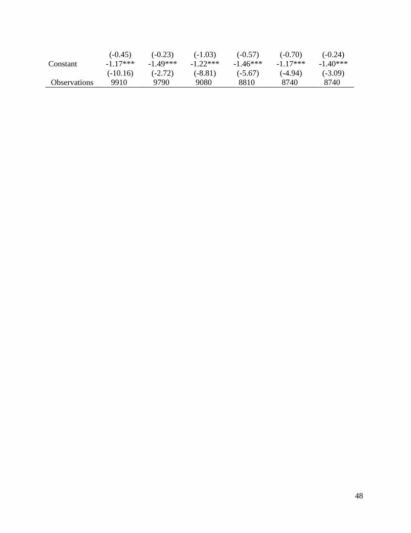
48
(-0.45) (-0.23) (-1.03) (-0.57) (-0.70) (-0.24) Constant -1.17*** -1.49*** -1.22*** -1.46*** -1.17*** -1.40*** (-10.16) (-2.72) (-8.81) (-5.67) (-4.94) (-3.09) Observations 9910 9790 9080 8810 8740 8740