DNB Working PaperAssessing bank competition for consumer loans

Wilko Bolt and David Humphrey

No. 457 / January 2015

De Nederlandsche Bank NV P.O. Box 98 1000 AB AMSTERDAM The Netherlands

Working Paper No. 457

January 2015

Assessing bank competition for consumer loans

Wilko Bolt and David Humphrey * * Views expressed are those of the authors and do not necessarily reflect official positions of De Nederlandsche Bank.

Assessing bank competition for consumer loans∗

20 January 2015

Wilko Bolta and David Humphreyb

aDe Nederlandsche Bank, Amsterdam, The NetherlandsbFlorida State University, Tallahassee, U.S.A.

Abstract

We assess the competitiveness of the $400 billion dollar U.S. bank consumer loan market by

comparing results from different competition measures–HHI, Lerner Index, H-Statistic along

with three others, two of which are related to frontier analysis. These measures are typically

weakly related to one another and only half of them identify banks with the highest loan

price and spread as also being the least competitive. This is the opposite of what would be

expected. The most and least competitive banks are not located in the most populous states

and the largest banks are underrepresented. Overall, the HHI should not be used to indicate

competition.

Keywords: consumer loans, bank competition, frontier analysis.

JEL classification: G21, L80, L00.

∗Corresponding author: David Humphrey, Department of Finance, Florida State University, Tal-lahassee, FL 32306-1042 USA; +1-(850)-668-8226. Comments by Alan Isaac, Juan-Pablo Montero,the participants at the 77th IAES Conference 2014 in Madrid, and at 12th IIOC 2014 in Chicagoare acknowledged and appreciated. The views expressed are those of the author and do not nec-essarily represent the views of De Nederlandsche Bank or the European System of Central Banks.Email addresses: dhumphrey@business.fsu.edu, w.bolt@dnb.nl

1 Introduction

Bank loans generate more than half of all U.S. bank revenues and differ between business

and consumer loans in both size and borrower sophistication. Consumers are viewed as less

informed in financial matters and so are the focus of most state and federal legislation, as

well as regulatory concern. Consumer loans in this paper comprise loans to individuals for

household, family, and other personal expenditures–a $400 billion dollar market. This covers

personal loans, student loans, auto loans, and other installment loans or revolving credit

plans but excludes loans secured by real estate (mortgages) and credit card loans (which

are concentrated at the very largest banks). Concerns about financial services offered to

consumers, including all types of consumer loans, led Congress to establish the Consumer

Financial Protection Bureau (CFPB) when it passed the 2010 Dodd-Frank Wall Street Reform

and Consumer Protection Act.

Studies have shown that bank consumer loans are markedly less expensive than payday

loans, pawn shop loans, or auto title loans (Caskey, 2005; Stegman, 2007). Suppliers of non-

bank consumer loans justify their higher price by noting the higher credit risk and nonpayment

experience they incur and, as a result, suggest they do not make excessive profits given the

risks they face. This has found some support in the empirical literature (Flannery and

Samolyk, 2005; Skiba and Tobacman, 2007). Non-bank lenders also argue that were it not

for them, the low income and risky loan market segment would not generally be served by

banks. From this perspective, the bank and non-bank consumer loan markets are essentially

segmented by borrower risk. In addition, data on costs, profitability and prices of consumer

loans for non-banks are not available to be compared with regularly reported bank consumer

loan data. Thus we focus on competition among banks for consumer loans rather than on

competition among all suppliers of consumer loans.

Banking regulators and consumer non-profits tend to focus their attention on consumer

complaints, which largely deal with the seeming unfairness of or inadequate information on

charges associated with particular banking services. Some very recent examples relate to un-

clear or misleading statements in lending documents (CFPB, 2013c), the existence of certain

credit card fees and retroactive interest charges (Agarwal, et al., 2014), and the (largely) past

practice of ordering account overdraft events so as to maximize the number of separate over-

drafts an account holder pays for (CFPB, 2013b). Only the CFPB provides public information

on the consumer complaints they receive and the bank associated with the complaint. Such

information is not available from the Federal Trade Commission, the F.D.I.C., Comptroller

of the Currency, the Federal Reserve, or state banking regulators who also receive consumer

complaints.

An alternative that has had some success in more oligopolistic industries than banking,

1

has been to identify and later look more closely at manufactured products where prices seem

to be “too high” according to some mark-up measure (e.g., Lerner Index) or remain very

stable even though costs are fluctuating or major material input costs are falling (e.g., H-

Statistic). The use of the HHI by banking regulators to limit market concentration through

mergers and acquisitions is an example of attempting to prevent implicit price collusion (local

price leadership) and maintain a competitive environment that will keep prices from becoming

“too high” via market power or price collusion. As little consumer complaint information is

available, we focus on trying to identify banks with relatively higher consumer loan prices and

report information on their market characteristics, such as where they are located, the income

level in their markets, the degree of branch ownership concentration, and other descriptives.

Rather than looking at the HHI as banking regulators do or at the Lerner Index or H-

Statistic (as academics tend to do), bank competition measures and their association with

relatively high consumer loan prices are assessed using three standard competition measures

(HHI, Lerner Index, H-Statistic) along with three others, two of which are related to frontier

analysis. The goal is to see how closely these six measures are related to one another and

assess their ability to identify banks with relatively high prices of consumer loans which may

suggest possible price collusion or uncompetitive behavior.

These measures, while often significantly statistically related to each other for US banks,

are only weakly economically related to one another.1 Measured by adjusted R-square, 16

out of the 21 bivariate correlations among our competition measures are less than .10 while

all correlations with HHI are .01 or less. Thus, the competition indicators appear to measure

different aspects of competition. The issue then is, which measure(s) may best reflect the

price conduct aspect of bank competition for consumer loans? We suggest an answer to this

question, explain why the two most used theoretically justified measures differ in assessing

competition, and show how all the measures identify similar or different characteristics of the

most and least competitive banks making consumer loans.

In what follows, the six competition measures are defined and estimated in Section 2

using quarterly data on 2,644 U.S. banks making consumer loans over 2008-2010, a period of

financial stress for both banks and many consumers. Section 3 illustrates the degree to which

each competition measure generally, and at their frequency tails, are related to one another.

Characteristics of the most and least competitive banks for each competition measure are

outlined in Section 4. This illustrates how the average loan price, bank profitability, and

industry asset share vary when moving from most to least competitive institutions for each

competition measure. For some measures, price and profitability falls (rather than rises)

as we move from the most competitive to the least competitive banks, not an encouraging

result. Section 5 seeks to determine the most useful measure(s) of consumer loan competition

1Our large sample size facilitates the former but not usually the latter.

2

based on the association of each measure with consumer loan price conduct that most would

associate with potentially competitive versus uncompetitive behavior. This measure is then

used in Section 6 to show which states appear to have the greatest concentration of most/least

competitive banks and note the average per capita income level of the communities they serve.

Section 7 presents our conclusions and their implication for policy.

2 Measures of Consumer Loan Competition

The banks in our sample all have more than $100 million in assets and accounted for 89% of

the types of consumer loans we cover.2 Our competition measures reflect the value weighted

average of all the locations a bank operates in. This is local, or at most regional, rather

than national since the median bank has branches in only two Metropolitan Statistical Areas

(MSAs) out of 956.3 Although the billion dollar banks in our sample have a broader geo-

graphical representation, the median billion dollar bank has branches in only four MSAs and

operates in only 1 state out of 50. Even at the 99th percentile, the average billion dollar bank

has offices in only 26 states.4

2.1 Market Concentration Measure: HHI

Regulators rely on the Herfindahl-Hirschman Index (HHI) because they believe it to be pre-

dictive of higher prices if mergers or acquisitions occur where market concentration exceeds a

certain level. It is also simple to compute.5 While the sum of squared market shares only

reflects the potential for uncompetitive or collusive behavior leading to higher prices and/or

greater profits, stock market event studies of proposed mergers have indeed supported that

view (e.g., Warren-Boulton and Dalkir, 2001). In practice, the HHI is augmented with ad-

ditional market information (U.S. Department of Justice, 2010). Importantly, and unlike

other measures of market competition, a post-merger/acquisition HHI can be determined and

inferences drawn as to likelihood of post-merger price increases if the merger goes through.

The other measures are solely ex post, not also ex ante as is the HHI. Even so, the focus on

2The sample includes 380 large banks each with assets over $1 billion and 2,264 banks with assets between$100 million and $1 billion. Although there are some 3,800 small banks with assets less than $100 million,they were excluded from the analysis as they only accounted for 11% of consumer loans and their mean sizewas less than that of a single branch office of a large bank.

3MSA refers to both the larger standard MSAs as well as the smaller non-MSA counties covered in theFDIC’s annual Summary of Deposits.

4Various screens were applied to eliminate shell banks, special purpose banks, banks with no loans, or nodeposits, or no full time employees, etc., or that contained variables beyond five standard deviations from themean and are clearly unrepresentative of the banking industry in general.

5In banking, the FDIC collects branch level deposit data to compute the HHI. Other measures would alsobe relatively simple to compute if the requisite cost accounting data were collected at the branch (or bank)level.

3

market shares does not account for how these shares may have been achieved–through lower

costs or by uncompetitive behavior. If lower costs and/or greater cost efficiency have been

an important reason for some banks in achieving a relatively high HHI, this will overstate

the apparent lack of competition that exists currently. It can also overstate the potential

uncompetitive effects of a bank merger, for example as suggested by an event study, if the

merger/acquisition is perceived to lead to important cost reductions which could be the main

reason behind a favorable event study result.

This possibility, originally raised by Demsetz (1973), led to the efficient structure contro-

versy and the finding that cost efficiency (measured from a cost frontier) and the HHI are

about equally important in explaining differences in bank profitability (Berger, 1995). Thus

greater predictive accuracy could be achieved in assessing the relationship of the HHI with

profitability after the influence of cost efficiency is “subtracted” or otherwise accounted for.

Studies showing that the HHI is generally associated with higher loan rates and lower deposit

rates (as surveyed in Dick and Hannan, 2010) are similarly affected since they too are not

adjusted for differences in efficiency across banks. Cost efficiency differences associated with

productivity differences and operating scale can affect observed factor input prices and hence

the pricing of deposit services as reflected in the deposit interest rate.

Following Hirtle (2007), a deposit-based HHI is determined for each of the 2,644 commercial

banks for 2010 in each of the 956 MSAs. These MSA HHIs are then weighted by each

bank’s deposit share across all the MSA’s the bank operates in to give a bank-level HHI.

Unfortunately, only deposit information is collected at the branch level across MSAs, not

the value of consumer loans (although the level of consumer loans should be related to the

level of deposits).6 Our bank-level HHIs are weighted averages of branch-level deposit data

and, as averages, can understate or overstate individual branch-level effects in different MSAs.

However, a bank-level HHI is needed in order to compare the HHI with the other competition

measures for which data are only available at the level of an individual bank.

The U.S. Justice Department’s 2010 horizontal merger guideline suggests that markets

with an HHI below 1,500 can be considered to be unconcentrated. A moderately concentrated

market exists when the HHI lies between 1,500 and 2,500 while a highly concentrated market

has a HHI above 2,500. While Table 1 shows that the average HHI for our 2,644 banks is

1,165 and thus at the bank-level operate in unconcentrated markets, the quartile of banks with

the largest HHI has an average value of 2,127 and as a group would be considered moderately

concentrated. Overall, only 4% of banks are in highly concentrated markets with an HHI

≥ 2,500. Banks that operate in highly concentrated markets have market power and could

use that power to charge prices well above underlying costs or engage in other uncompetitive

behavior. This is by no means certain but would bear further investigation of banks so

6The Appendix has more information on the calculation process.

4

identified. Had we used the 1992 DOJ guidelines, the percent of banks in highly concentrated

markets (HHI ¿ 1,800) would be 16% but the guidelines were liberalized in 2010.

2.2 Level of the Price-Cost Spread: Lerner Index

Academics have for solid theoretical reasons favoured the Lerner Index (Lerner, 1934) which

seeks to measure realized competition as opposed to the potential for competition as does the

HHI. The Lerner Index reflects the percentage spread of the output price or average consumer

loan interest rate (Po) to estimated marginal cost (MC) for individual banks averaged over

2008-2010: (Po − MC)/Po. Marginal cost is estimated from a logarithmic cost function

lnC = f(lnQo, lnPi) where C is total cost, Qo is output, Pi is composed of funding, labor, and

capital input prices, and MC =∑

i(∂ lnC/∂ lnQo)(C/Qo). As scale economies (SCE) are the

ratio of marginal to average cost (AC), the Lerner Index can be simplified to Po−AC ·SCE.7

This reflects the level of the price-cost spread.

It is not possible to estimate a Lerner Index directly for consumer loans using a cost

function since total cost is not reported. Although one can reasonably approximate the

average interest expense incurred in making consumer loans, the allocation of operating costs

(labor, physical capital, and other non-interest expense) to consumer loans is not reported.

Consequently, a standard Lerner Index was estimated for the whole bank and is used in place

of a Lerner Index specific to consumer loans which is not available. Fortunately, this data

limitation does not apply to three of the remaining competition measures (but does apply to

the adjusted Lerner measure below). Our specification of the Lerner Index is shown in the

Appendix and its average value is 39% in Table 1. The quartile of most competitive banks–

those with the lowest Lerner Index–have a mean value of 25% while the least competitive

quartile has a mean of 51%. To put these values in perspective, if MC was .03 the loan rate

Po would average .049 and range between .040 and .061.

[Insert Table1 here]

2.3 Changes in the Price-Cost Spread: H-Statistic

Like the Lerner Index, the H-Statistic of Panzar and Rosse (1987) is based on economic theory

and seeks to measure realized competition. The H-Statistic relates changes in total consumer

loan revenue (TR = PoQo) to changes in observed input prices (Pi) holding output level (Qo)

constant and is shown in the Appendix. In contrast to the Lerner Index, the H-Statistic is

based on an estimated revenue function lnTR = g(lnPi, lnQo). The H-Statistic itself is the

7As the variation of this unit spread across banks will accord well with its percentage value if divided byPo or AC, in this illustration we focus on the spread alone.

5

sum of partial derivatives or elasticities:∑

i ∂ lnTR/∂ lnPi and reflects the change in output

price to input prices (∂Po/∂Pi) since output is being held constant. Banks with a high ratio

of changes in output to input prices ∂Po/∂Pi will also have a large difference in these prices

∂Po − ∂Pi so the latter is an alternative expression of the former.

If output and inputs prices rise and fall together over time or across banks the implication

is that non-cost influences on output price are small indicating a competitive market where

cost determines price. Competition is strong when the H-Statistic is close to 1.0 and non-

existent when it is close to 0.0. The closer the H-Statistic is to zero, the lower the influence

of cost on output price, implying that firms are able to set price independently from cost as

a result of having and using market power to set prices or collude with others to do so.

The average H-Statistic for bank consumer loans in Table 1 is .87, which is not very distant

from 1.0 and is suggestive of a relatively competitive market. The quartile of banks with the

lowest H-Statistics have an average value of .79 which is still quite far from zero and, by

itself, would not indicate a serious lack of competition although this is a judgement call as

no standard exists unless an H-Statistic is close to either 1.0 or 0.0–the two extreme values.

At least with the HHI, the Justice Department provides a guideline (although one that has

changed over time). While subjective judgement is also used in assessing the Lerner Index, a

guideline of sorts exists in the values of this index (or mark-up) in other industries.

2.4 Comparing the Lerner Index with the H-Statistic

Assuming that average cost reflects the weighted average of input prices (Pi), the two compe-

tition measures favored by academics–for comparison purposes–can be expressed as:

Lerner Index Po − AC · SCE (Level of the price-cost spread)

H-Statistic ∂Po − ∂AC (Change in the price-cost spread).

In effect, the Lerner Index looks at the average level of the price-cost spread over a sample

period while the H-Statistic looks at changes in that spread: they measure different aspects

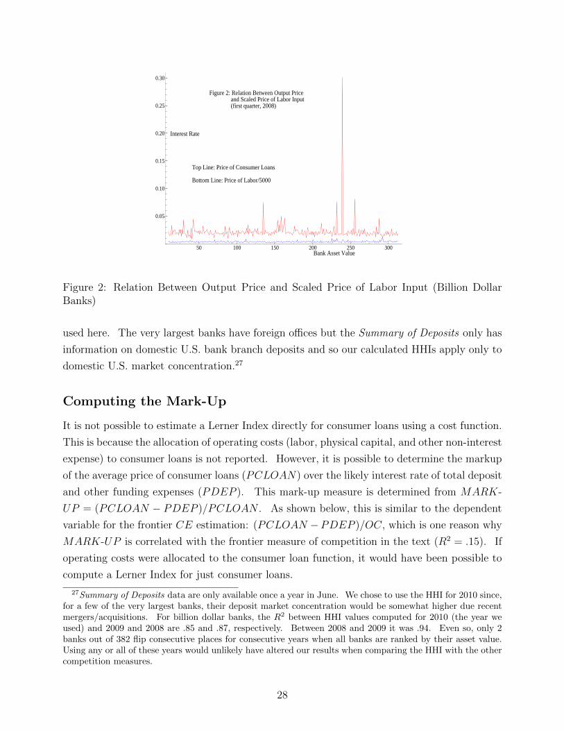
of competition. This difference is illustrated in Figures 1 and 2. In both figures, the top line

represents the variation in the price of consumer loans (an interest rate) for billion dollar banks

in the first quarter of 2008 arrayed by the value of bank assets on the X-axis. The bottom

line in the first figure shows the variation in the price of deposits and other funding (also an

interest rate) for the same banks in the same quarter. In the second figure, the bottom line

reflects the scaled price of labor (annual wages and benefits in thousands of dollars divided by

5,000 for comparison purposes).8

[Insert Figure 1 here]

8In a double log estimating equation, the scaling would only affect the intercept, not the slope of therelationship between output and input prices. Thus the H-Statistic is unaffected with or without scaling.

6

The H-Statistic reflects the sum of the strength of the covariation between the price of

consumer loans (the top line in the figures) and of the specified input prices (bottom line). A

strong relationship suggests that costs determine prices rather than market power or collusion.

Although the Lerner Index is a measure of the spread between the price of consumer loans

and the sum of the input prices (marginal or average cost) per unit of output, the H-Statistic

is only concerned with their covariation.9 The HHI, in contrast, uses market structure to

infer price conduct and/or profit performance but does not directly measure either one.

[Insert Figure 2 here]

In our data set, regressing the Lerner Index on the H-Statistic gives an R2 = .09 indicating

they are only very weakly related to each other. Thus they reflect different aspects of com-

petition: a price-cost markup or spread for the Lerner Index and a measure of possible price

collusion for the H-Statistic. Banks identified by the Lerner Index as having high prices will

differ from banks so identified by the H-Statistic.

2.5 Mark-Up Over Deposit Costs

While the Lerner Index reflects the mark-up for the entire bank, a more limited measure is

possible for consumer loans. This would relate the average price of consumer loans (PCL)

to the average cost of deposits that fund these and other loans (PDEP ) and is expressed as

(PCL −PDEP )/PCL.10 The average mark-up of price over deposit costs for consumer loans in

Table 1 is 77% and varies from 66% to 86% across quartiles. The mark-up appears high for

two reasons: interest rates are at historical lows during our sample period and the numerator

of the Mark-Up excludes operating costs. Whether this spread is deemed excessive, suggesting

a lack of competition, depends on the spread earned by other banks for their consumer loans

and the return on equity in other industries.

2.6 L, a Lerner Index Adjusted for Inefficiency

A Lerner Index adjusted for cost and profit inefficiency has been proposed and used by Koetter,

Kolari, and Spierdijk (2012) to gauge the possible effect of banking deregulation on banking

competition. If banks with market power choose the “quiet life” rather than seeking to

minimize costs and, given quantities, have the opportunity to set prices to maximize profits,

then reported costs will be higher and profits lower than otherwise and in this sense reflect

“inefficiencies”. A preference for the quiet life if competition is weak can be one reason

9Either measure can be estimated with cross-section, time-series, or panel data.10PDEP is the presumed average cost of funding consumer loans. In practice, it is close to the marginal

funding cost as almost all bank funding is short term.

7

for inefficiency but others exist as well. Not all bank branches can be located in faster

growing and higher income areas even though, if they were, loan revenues and profits would

be higher since higher income areas tend to generate more loan demand and branch networks

support more low cost deposits per office. Also, not all banks adopt to the same degree

cost saving innovations such as replacing branches with ATMs, using peak-load/part-time

staffing, applying artificial intelligence in assessing loan applications, monitoring as carefully

outstanding loans, or promoting lower cost internet banking. Banks also differ in managerial

talent, loan officer skill, loan workout procedures, board oversight, and in their mix of funding

sources and loan concentrations, all of which are known in the industry to affect cost and

profitability. As most of these influences are not subject to effective measurement, their

relative contribution to measured inefficiency is a judgement call. Weak competition is just

one possibility.

The cost function used to estimate MC for the adjusted Lerner Index, L, is specified

the same way as the function to obtain MC for the unadjusted Lerner Index above but is

estimated using a Stochastic Frontier Approach (SFA) rather than OLSQ. Although the

resulting MC is not very different, SFA estimation generates an estimate of cost inefficiency

from the composed error residuals of the cost function. An alternative profit function, which

takes quantities as given and maximizes output price (rather than taking market price as

given and maximizing quantity) is also estimated using SFA to obtain an estimate of profit

inefficiency. The separation of inefficiency from normally distributed error in these cost and

profit models is achieved by assuming inefficiency is distributed as a half normal distribution

so that most banks will lie on or close to their cost or profit frontiers.

In simple terms, the adjusted Lerner Index substitutes a cost and profit “efficiency cor-

rected” price (P ∗o ) for the observed price (Po) in a standard Lerner Index giving L = (P ∗

o −MC)/P ∗

o . The efficiency adjusted price P ∗o is derived from the predicted values of the SFA

estimated cost and alternative profit functions since predicted cost and profit will differ from

their observed values by the amount of SFA estimated inefficiency, suggesting that costs could

be lower and profits higher if inefficiency did not exist. These predicted costs and profits are

summed to predict revenues and, divided by the value of banking output produced (all loans

plus securities in the model), gives P ∗o .11

As seen in Table 1, we find the adjusted Lerner Index to be larger than an identically

specified measure–L2–estimated using OLSQ rather than SFA, so it is not adjusted for cost

or profit efficiency. This difference should indicate the extent that bank costs are not as low

or profits not as high as that for the frontier bank with the lowest cost or highest profit in the

11Using our data, predicted revenues are 23% less than observed revenues (TR) while the sum of bankingoutput produced is 27% less than total assets (TA). Output price Po in the standard Lerner Index is avergerevenue per dollar of assets or TR/TA. The lower values used in P ∗

o largely offset each other when L isestimated using OLSQ rather than SFA so at the data mean P ∗

o ≈ Po.

8

sample. Profit inefficiency turns out to be much more important in determining the difference

between L and L2 than is cost inefficiency both here and in Koetter, Kolari, and Spierdijk

(2012). Even so, the difference in average values between L and L2 in Table 1 is not large

since the R2 between them is .93 in Table 2.

Banks view themselves as attempting to control costs even if they are unable to lower

them to the level of the most cost efficient bank on the frontier. Thus a cost-minimizing,

price-taking model is a more reasonable economic framework than one of monopsony with

strong bank control over input prices. Consistency suggests that banks would also seek

to maximize profits even though not all will be as profitable as the bank with the highest

profits. If a standard profit function is specified, banks take prices as determined in the

market and seek to maximize output. In such a framework profit inefficiency is conceptually

the deviation of observed profits from the maximum observed profit obtained by a bank on

the frontier, once operating costs, scale, market interest rates, and business cycle influences on

profits are controlled for. This is similar to how cost inefficiency is obtained but is different

from the alternative profit function used to construct L and L2 since output levels are taken

as given and the bank is a output price-setter (not a price-taker). Here profit inefficiency

is conceptually the deviation of observed profits from what they could be under monopoly.

In reality, banks face markets where price-taking is a more accurate assumption (business

loans, securities holding and trading, standard payment and deposit services) than a degree of

price-setting behavior (consumer loans, specialized payment services, investment banking and

off-balance-sheet activities). Choosing one approach over the other is difficult for the entire

bank since different services seem to fit different behavioral models.

2.7 Adjusting Revenues for Costs: A Competition Efficiency (CE)

Frontier

Using a different procedure based on efficient frontier analysis, it is possible to derive infer-

ences of bank consumer loan competition from estimating a revenue-cost competition fron-

tier. We also suggest that standard competition measures incompletely adjust for important

cost/productivity differences among banks and incorporate these additional cost influences

into our analysis (Bolt and Humphrey, 2010 and 2012). Our frontier approach to measuring

competition is similar to that developed independently by Boone (2008). Thus our focus is

on an empirical specification of a Boone-type model which was shown theoretically to be more

robust than the price-cost margin of a Lerner Index.12

12Boone’s aim was to determine competition based on a firm’s profits. The degree of competition isdetermined by subtracting a firm’s variable costs from its revenues. This gives an implied (residual) returnto fixed inputs plus extra revenues associated with the degree of relative competition.

9

In simple terms, profits = f (competition, costs). As profits are simply revenues minus

costs, profit differences across banks can be alternatively measured as the “mark-up” ratio

of revenue to costs and, if all explicit costs are included, an estimate of relative competition

can be obtained from: revenue/costs - f (costs) = g (competition). Here g (competition)

represents the unexplained mark-up over cost and includes a normal return on equity which

is not explicitly specified in the model. Our revenue/cost ratio is the inverse of the popular

Cost Income Ratio used in banking or revenue/cost = (interest revenue - interest expense +

fee income)/(labor + capital + other non-interest expense). Banks with a lower input cost

per unit of output revenue raised are (by definition) more profitable. This approach is similar

to using a Lerner-type Index expressed as the ratio Po/MC, replacing MC with AC, and

multiplying by a ratio of output and input quantities Qo/Qi giving: (Po ∗Qo/AC ∗Qi) which

equals a revenue/cost ratio.13

If the productivity of inputs Qi differs across banks then input prices (reflected in AC)

will not reflect their true cost to the bank. Observed input cost AC ∗ Qi will be higher

for banks with greater productivity making them appear more competitive than they are

as the observed spread Po − MC or Po − AC will be lower. The productivity variables

we specify have been important in reducing cost inefficiency to low levels in both stochastic

and linear programming frontier models (Carbo, Humphrey, and Lopez del Paso, 2007).14

Specifically, labor (L) is more productive and real labor costs are lower when there are fewer

employees (line, back office, and management) per branch office (BR). As well, capital

productivity is improved when a bank produces more deposits (DEP ) per branch office.

Banks differ in their staffing arrangements (L/BR) to meet their daily peak load for teller

window transactions, back office transaction processing, and in their layers of management.

Some banks operate in-store or supermarket branches where the staffing level is about half that

of a stand-alone office (Radecki, Wenninger, and Orlow, 1996). In addition, in-store and stand-

alone branches located in higher income areas (suburban versus central city or rural) generate

more deposits per office, raising the deposit/branch ratio (DEP/BR) as well as generating a

greater demand for other banking services (adding to revenue). Importantly, branch locations

in high income areas are limited and in-store branch contracts with supermarket chains are

exclusive within states or metropolitan areas so these productivity/cost differences can be

relatively persistent.15 In sum, a high labor/branch ratio and a low deposit/branch ratio

13Expressing the Lerner Index as a mark-up percentage (Po−MC)/Po, a spread Po−MC or a ratio Po/MCshould give the much the same ranking of bank competition. This is also the case when average cost ACreplaces marginal cost since MC is uniquely tied to AC by the slope of the supply curve (or scale economies).We do not have separate information on Qo/Qi, only the reported revenue/cost result.

14Berger and Mester (1997) and Frei, Harker, and Hunter (2000) have also shown productivity influences tobe a primary determinant of previously unexplained bank cost inefficiency.

15The capital cost of an in-store branch is only about one-fifth of a conventional branch (Radecki, Wenninger,and Orlow, 1996).

10

suggests cost inefficiency that rolls over into profit inefficiencies relative to other banks.

In estimating the competition frontier, we use the composed error Distribution Free Ap-

proach (DFA) in Berger (1993).16 In a composed error framework, the DFA model illustrated

in (1) relates the ratio of consumer loan revenues, net of funding expenses, to overall oper-

ating costs. Specifically, it attempts to explain the variation across banks in the ratio of

unit consumer loan revenues (PCLOAN) minus unit deposit cost (PDEP ) divided by overall

operating cost (OC), comprised of labor, physical capital, and materials expense. Although

operating cost is not allocated to the various banking services in the reported data, we do spec-

ify variables to explain the overall level and variation of operating cost among banks which,

in turn, influence the effect of operating cost on consumer loans and other banking services.

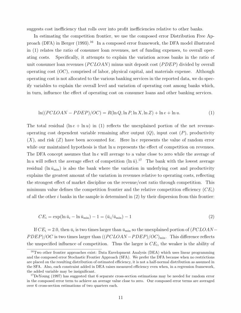
ln((PCLOAN − PDEP )/OC) = R(lnQ, lnP, lnX, lnZ) + ln e+ lnu. (1)

The total residual (ln e + lnu) in (1) reflects the unexplained portion of the net revenue-

operating cost dependent variable remaining after output (Q), input cost (P ), productivity

(X), and risk (Z) have been accounted for. Here ln e represents the value of random error

while our maintained hypothesis is that lnu represents the effect of competition on revenues.

The DFA concept assumes that ln e will average to a value close to zero while the average of

lnu will reflect the average effect of competition (ln u).17 The bank with the lowest average

residual (ln umin) is also the bank where the variation in underlying cost and productivity

explains the greatest amount of the variation in revenues relative to operating costs, reflecting

the strongest effect of market discipline on the revenue/cost ratio through competition. This

minimum value defines the competition frontier and the relative competition efficiency (CEi)

of all the other i banks in the sample is determined in (2) by their dispersion from this frontier:

CEi = exp(ln ui − ln umin) − 1 = (ui/umin) − 1 (2)

If CEi = 2.0, then ui is two times larger than umin so the unexplained portion of (PCLOAN−PDEP )/OC is two times larger than ((PCLOAN−PDEP )/OC)min. This difference reflects

the unspecified influence of competition. Thus the larger is CEi, the weaker is the ability of

16Two other frontier approaches exist: Data Envelopment Analysis (DEA) which uses linear programmingand the composed error Stochastic Frontier Approach (SFA). We prefer the DFA because when no restrictionsare placed on the resulting distribution of estimated efficiency, it is not a half-normal distribution as assumed inthe SFA. Also, each constraint added in DEA raises measured efficiency even when, in a regression framework,the added variable may be insignificant.

17DeYoung (1997) has suggested that 6 separate cross-section estimations may be needed for random errorin the composed error term to achieve an average value close to zero. Our composed error terms are averagedover 6 cross-section estimations of two quarters each.

11

market competition to restrain revenues, relative to costs, so CE is similar to inefficiency in

a cost frontier. Unlike the L measure above, we do not incorporate profit inefficiency from

either a standard or alternative profit function. We focus on how well–or poorly–the compe-

tition measures are related to relatively high prices for that is what the consumer pays. If

high prices lead to high profits then focusing on high prices will identify banks that do both.

We see no reason to penalize those that achieve relatively high profits without having high

prices, for example by controlling better their costs or being located in SMSAs with higher

than average growth or income which affects the demand for consumer loans.

Although we account for the output level of consumer loans, factor prices, factor produc-

tivity, risk, scale effects, and the stage of the business cycle, it is still possible that we have

excluded some important cost influence from the estimated frontier model shown in the Ap-

pendix. Even so, our statistical fit across six two-quarter panel estimations averaged .86,

suggesting that there is not much left to be explained by unreported and excluded differences

in cost.18 Indeed, if all costs have been included, this suggests that 14% of the variation in

(PCLOAN − PDEP )/OC reflects the influence from (unobserved) competition. If all costs

have not been included, then the influence of competition is smaller than 14% and we have

overestimated, rather than underestimated, the influence of a lack of competition.

As seen in Table 1, the average consumer loan CE value for 2,644 banks is 9.6, which

reflects the fact that the mean bank experienced a level of averaged unexplained residuals

from (1) across six cross-section regressions that were 9.6 times the level of those for the bank

whose averaged residuals were lowest (and hence define the competition efficiency frontier).

This is a relative measure so if the minimum residual is small, the CE value can still appear

to be large as an index.

[Insert Table 2 here]

3 Similarity Among Competition Measures

The fact that the Lerner Index and the H-Statistic appear to measure different aspects of

competition was illustrated above. Unfortunately, this seems to be a general result that

applies to almost all of the competition indicators used here according to the adjusted R-

squares shown in Table 2. Neglecting L2, as it is so similar to L, out of the 15 bivariate

correlations among the remaining six measures, only 3 are larger than .10. These three

18While a fixed effects approach would likely improve the statistical fit, the time and bank-specific dummyvariables can not discriminate between excluded cost effects (which we would like to include) and the excludedeffect of competition on revenues (which we wish to exclude and keep in the residual). The Lerner Index hasa similar problem when applied to the entire bank as it excludes around 35% of revenue generated by bankingoutput when estimating marginal cost in a cost function as output associated with non-interest income is notreported.

12

concern the Lerner Index with Mark-Up (.11), Mark-Up with CE (.15) and the Lerner Index

with the adjusted Lerner measure L (.50). The four measures here–Lerner Index, L, Mark-up,

and CE–are variations on the spread between revenue and cost. Importantly, all correlations

with the regulator-favored HHI measure are .01 or less while the relationship between the two

often used academic measures–Lerner Index and H-Statistic–is only .09.

[Insert Table 3 here]

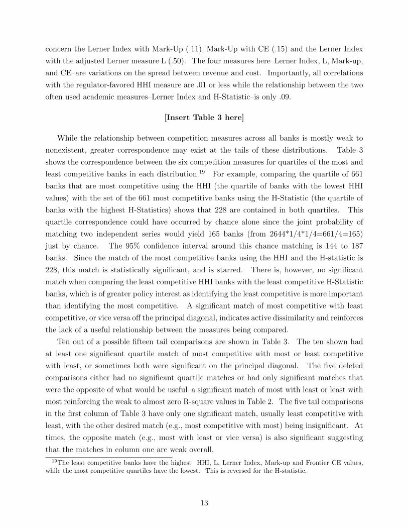
While the relationship between competition measures across all banks is mostly weak to

nonexistent, greater correspondence may exist at the tails of these distributions. Table 3

shows the correspondence between the six competition measures for quartiles of the most and

least competitive banks in each distribution.19 For example, comparing the quartile of 661

banks that are most competitive using the HHI (the quartile of banks with the lowest HHI

values) with the set of the 661 most competitive banks using the H-Statistic (the quartile of

banks with the highest H-Statistics) shows that 228 are contained in both quartiles. This

quartile correspondence could have occurred by chance alone since the joint probability of

matching two independent series would yield 165 banks (from 2644*1/4*1/4=661/4=165)

just by chance. The 95% confidence interval around this chance matching is 144 to 187

banks. Since the match of the most competitive banks using the HHI and the H-statistic is

228, this match is statistically significant, and is starred. There is, however, no significant

match when comparing the least competitive HHI banks with the least competitive H-Statistic

banks, which is of greater policy interest as identifying the least competitive is more important

than identifying the most competitive. A significant match of most competitive with least

competitive, or vice versa off the principal diagonal, indicates active dissimilarity and reinforces

the lack of a useful relationship between the measures being compared.

Ten out of a possible fifteen tail comparisons are shown in Table 3. The ten shown had

at least one significant quartile match of most competitive with most or least competitive

with least, or sometimes both were significant on the principal diagonal. The five deleted

comparisons either had no significant quartile matches or had only significant matches that

were the opposite of what would be useful–a significant match of most with least or least with

most reinforcing the weak to almost zero R-square values in Table 2. The five tail comparisons

in the first column of Table 3 have only one significant match, usually least competitive with

least, with the other desired match (e.g., most competitive with most) being insignificant. At

times, the opposite match (e.g., most with least or vice versa) is also significant suggesting

that the matches in column one are weak overall.

19The least competitive banks have the highest HHI, L, Lerner Index, Mark-up and Frontier CE values,while the most competitive quartiles have the lowest. This is reversed for the H-statistic.

13

The five matches shown in the second column are all much stronger since the match of

most competitive with most and least competitive with least on the principal diagonal are both

significant while all off-diagonal matches are insignificant. Neither the HHI or the H-Statistic

are represented here. Rather, the strongest relationships are among the four measures–Lerner

Index, L, Mark-Up, and Frontier CE measures that are, in different ways, based on a price-cost

spread. These results are unchanged even if when comparisons are made using the highest

and lowest deciles (90% and 10%, not shown).

The fact that there is only a relatively weak correspondence between banks identified as

being most or least competitive using the HHI and the other measures, suggests that an effort

to benchmark the HHI to more theoretically (and, as we see next, empirically) supported

measures appears problematic.

[Insert Table 4 here]

4 Characteristics of Most and Least Competitive Banks

Across Competition Measures

A useful measure of bank competition should be able to identify banks that have relatively

high prices due to a lack of competition in the output market, rather than being due to higher

input costs, a lower scale of operation, lower productivity, etc. If output prices are high

due to high costs resulting from a lack of competition (a “quiet life” view), controlling for

differences in costs across banks would likely reduce the ability of most of our competition

measures to identify banks with relatively high output prices. With the exception of HHI, the

other measures attempt to control for observed or estimated cost differences–the H-Statistic

by covariation with output price while the spread indicators (Lerner Index, Mark-up, Frontier

CE) effectively subtract cost from price. The L measure corrects for cost and profit inefficiency

before subtracting cost from price. At the limit, not subtracting any cost gives just price

which is a perfect predictor of observed price. Our view is that all identifiable costs should

be subtracted from price or revenue while the view of Koetter, Kolari, and Spierdijk (2012)

who developed L, is that frontier analysis can be used to adjust price (correcting it for both

cost and profit inefficiency) while estimating MC using a SFA framework. The result is that

L has a larger spread than L2 but a lower one than a standard Lerner Index (due to how the

price and marginal costs are defined).

Table 4 illustrates how all of our competition indicators are associated with bank char-

acteristics that are often cited as suggesting a lack of competition. This concerns consumer

loan prices, a consumer loan-deposit rate spread (profitability), and the overall return on bank

14

assets (ROA).20 Each competition measure has been ranked from most to least competitive

with the average quartile values shown in the first seven rows of Table 4. As expected, all but

the H-Statistic steadily rise in value when moving from quartiles of most to least competitive

banks associated with these measures.

Rows 8 to 14 show how the average consumer loan rate of the banks in each of the quartiles

of each competition measure in rows 1 to 7 varies from most competitive (where the loan rate

should be lowest) to least competitive (where the loan rate should be highest). As summarized

in the last column, the relationship is negative for the HHI, the H-Statistic, L and L2. The

banks these four measures identify as being least competitive have lower consumer loan rates

than the banks they identify as being most competitive. This is the opposite of what we

would expect and indicates, at least for consumer loans, that these measures should not be

relied upon to identify banks with high prices. The expected positive relationship is seen only

for the Lerner Index, Mark-Up, and Frontier CE measures. Here the average loan rates of

banks they identify as most competitive are lowest while the loan rates of banks identified as

least competitive are highest. The same results are obtained when the competition measures

are related to bank consumer loan-deposit rate spreads (rows 15 to 21)21

In terms of overall bank profitability (net income/asset ratio), banks that the HHI and

the H-Statistic identify as being the least competitive are less (not more) profitable than the

banks they identify as most competitive. The banks these two measures identify as being

the least competitive have the lowest consumer loan rates, the lowest rate spreads, and the

lowest profits and all three are the opposite of what a useful competition measure is expected

to show. The adjusted Lerner Index L, along with L2, correctly predicts profitability but not

consumer loan rates or the loan-deposit rate spread. The three remaining measures (Lerner

Index, Mark-up, and Frontier CE) consistently give the expected results. It would be nice if

these three measures also identified the same banks for each of the competition quartiles, but

they don’t. The share of our sampled bank assets placed in the most competitive quartile

by the Lerner Index is 83% with an asset share of only 5% for banks deemed to be least

competitive. This suggests that the vast majority of banks are competitive (last column of

Table 4). As the quartile of most competitive banks using the Mark-Up measure accounts

for only 10% of bank assets but 48% of assets for the least competitive quartile, this measure

suggests that half of the banking industry is not very competitive. Finally, the Frontier CE

measure would place some large banks in both the most and least competitive categories–a

20Using Call Report identifiers, the price of consumer loans is PCLOAN = RIADB486/(RCFDB539 +RCFD2011) while the loan price-deposit rate spread is CSPREAD = PCLOAN - [(RIAD4073 - RIAD4185 -RIAD4200)/(RCFN2200 + RCON2200 + RCONB993 + RCFDB995)].

21The exception is the HHI since the rate spread does not vary between banks deemed most or leastcompetitive using this measure.

15

more heterogeneous distribution.22 At this point, it is not possible to say whether small or

large banks are generally least competitive or have the highest consumer loan prices since the

three competition measures that seem to perform best in Table 4 give differing results in this

regard. This set of three can be narrowed further.

[Insert Table 5 here]

5 Selecting A “Favored” Competition Measure

One way to assess the differing results in Table 4 would be to place more confidence in those

competition measures that closely accord to what most would accept as indicating a lack of

competition. Namely, relatively high prices, a higher spread, and higher profitability. Only

the Lerner Index, Mark-up, and Frontier CE measures meet all three of these criteria. We

now assess the ability of these three and the other measures to actually identify banks with

relatively low versus high loan output prices. This is viewed as a indicator of the strength

versus weakness of market competition so that the greater the match, the greater the possible

accuracy of the measure.

Using the same methodology as Table 3, Table 5 shows the number of matches and their

significance for six competition indicators.23 The left hand side of Table 5 shows that the

quartile of banks identified by the HHI, H-Statistic, and L measures as being most (least)

competitive do contain some banks that do have the lowest (highest) consumer loan prices.

However, the number is less than that needed to be significantly different from a match by

chance alone (at the 95% level of confidence). That is, out of 661 possible matches on each

of the two principal diagonal elements, the number of matches is less than 187 which is the

upper bound to attain significance. None are significant using the HHI and, while there

are statistically significant matches for the H-Statistic and L, they are not on the principal

diagonal and thus are the opposite of what is desired.24

The remaining three competition measures on the right hand side of Table 5–Lerner In-

dex, Mark-Up, and Frontier CE–all have significant matches on the principal diagonal (with

insignificance off the diagonal), which is what is desired. Of the quartile of banks that

are identified by the Lerner Index as being most competitive (those having the lowest index

value), 231 banks out of a possible 661 also have the lowest price of consumer loans. As the

number of matched banks is larger than 187, this is a significant match. When the Lerner

22The HHI, and especially the H-Statistic, would place most or almost all large banks in the least competitivequartiles.

23The L2 measure is excluded since it is so similar to L.24This reinforces the result seen in Table 4 for these three measures.

16

Index is supposed to identify the set of least competitive banks which should have the high-

est loan price, the match is insignificant. Since both elements on the principal diagonal for

the Mark-Up and the Frontier CE measures are significant, they both appear to do a better

job in distinguishing more competitive from less competitive banks. Even so, the Mark-up

has absolutely fewer matched banks on the principal diagonal compared to the Frontier CE.

The results of Table 5 are not improved when, instead of quartiles, we look at the 10% and

90% decile matches in Table 6. The HHI, H-Statistic, and L measures still perform poorly

in having no significant matches on the principal diagonal while the matches for the Lerner

Index, Mark-up, and Frontier CE are significant as before with the same ranking in terms of

the number of bank matches.

One possible reason why the Frontier CE measure seems to do better at matching with loan

prices is that it controls for a broader selection of cost differences among banks. The Mark-

Up controls for average deposit/funding cost while the Lerner Index controls for marginal

cost, which should reflect the marginal influence of funding cost, input prices, and scale of

operation. In contrast, CE additionally controls for labor and branch productivity as well as

risk (loan losses and capital position).

[Insert Table 6 here]

Using the price of consumer loans as our benchmark indicator to assess the apparent

predictive accuracy of the various competition measures, the Frontier CE measure seems

to perform best–at least for consumer loans. However, an important practical consideration

would be ease of estimation. Here the Mark-up is much easier to obtain than either the Lerner

Index or the Frontier CE. Also, due to a lack of data, the Lerner Index was representative

of the entire bank while both the Mark-Up and the Frontier CE were specific to consumer

loans. We do not know if the Lerner Index would have had a more favorable outcome had

the requisite data on consumer loans been available. In any case, the Mark-up, defined as

the price of consumer loans minus the average cost of funding (deposits and other borrowed

funds) all divided by the price of consumer loans is really just a simpler Lerner Index without

the need to estimate a cost function. A caution here is that while both the Mark-up and

CE measures identify the most banks which do in fact have the highest loan rates, not all

the banks so identified the same banks. That is, some banks identified by the Mark-up as

having high consumer loan rates will not also be identified by the CE measure even though all

the banks identified by both measures are in the highest quartile or decile of banks with the

highest rates. Even so, the overlap here is substantial and ranges from half to three quarters

for these two measures in Tables 5 and 6.

17

6 Location of the Most/Least Competitive Banks

The sets of most and least competitive banks are not distributed randomly across the U.S.

Both sets of banks appear to be concentrated in smaller, less densely populated states, which

experience a range of per capita income levels. Ranking all 2,644 consumer loan banks by

their Frontier CE measure–the competition indicator that seemed to do the best in Tables

5 and 6, the decile of the most competitive banks (those with the lowest CE) are located in

Vermont, Delaware, New Jersey, Wisconsin, and Alabama. As a group, these banks operate

an average of 40% of all branches in these states. The decile of least competitive banks

are found in Montana, Wyoming, Louisiana, Oklahoma, and South Dakota and, as a group,

operate an average of 17% of the branches there. In these states, the set of most competitive

banks are twice as concentrated–in terms of branch ownership–than banks deemed as being

least competitive.

One might expect that per capita income in states where the least competitive banks are

located may be lower. It is, but only by 3%. Importantly, the income range in the two sets

of states noted above is quite similar so income differences are only weakly associated with

differences in apparent consumer loan competition. The five states where the most competitive

banks are concentrated have an annual per capita income range of $35,300 to $56,000 while

the range in the other five states where the least competitive banks are concentrated is similar

at $33,900 to $51,500. If the least competitive banks are indeed behaving in an uncompetitive

manner in terms of consumer loan prices, this behavior seems not to be concentrated in states

with markedly lower per capita income.25

It would be interesting to see which of the bank-specific consumer loan competition mea-

sures may be predictive of current regulator consumer loan concerns. For example, the

Consumer Financial Protection Bureau (CFPB) is concerned about certain bank short-term

consumer deposit advance (loan) products and non-bank payday consumer loan practices

(CFPB, 2013a). The Bureau is also concerned with bank deposit overdraft arrangements

that generated revenues of $32 billion in 2012 (CFPB, 2013b; Raice and Zibel, 2013). Ad-

ditional concerns have included bank mortgage and student loans as well as loan collection

procedures. Since the CFPB is a new organization, their sample of banks listed in the con-

sumer complaints is small and would have to be augmented with bank complaint data from

other agencies (which is not publicly available). Unfortunately, we are unable to make this

comparison.

25Publicly available data on consumer loan customer income by bank are not available so it is not possibleto determine if differences in customer per capita income are as small as they appear to be using state levelper capita averages.

18

7 Summary and Conclusions

Consumer loans account for $400 billion at U.S. banks and they have been a focus of con-

gressional legislation, Federal Trade Commission and Consumer Financial Protection Bureau

investigations, as well as banking regulator rules and guidance. This is because consumer

borrowers are both more numerous than business borrowers and are typically less sophisticated

in financial affairs so regulatory oversight can assist in achieving a fair outcome for consumer

borrowers in dealing with bank lenders. Identifying potentially unfair or uncompetitive be-

havior can arise through consumer complaints as well as from identifying institutions that

have relatively higher prices than their peers (after controlling for cost differences). This

is the goal of the indicators of competition presented here–HHI, H-Statistic, Lerner Index,

Mark-up, and a two newer measures based on frontier analysis.

Prior analyses have only compared the HHI with the Lerner Index or, separately, with the

H-Statistic. They have not really contrasted the latter two measures with each other and in

any case have looked at competition at the level of the entire bank. We compare competition

measures with each other at 2,644 banks over 2008-2010 using quarterly data. Ranking

banks from most to least competitive for each competition measure, we find that most of

them are only weakly related to each other. And there is no economic relationship between

these measures and the HHI as measured by R-square. Assessing competition appears to be

measure-specific. This holds overall and at the tails of the competition rankings.

The relationship between the various competition rankings of banks–from most to least

competitive–and their match with banks having (respectively) the lowest to highest average

price of consumer loans is strongest and significant for the Lerner Index, Mark-up (which is a

simpler Lerner Index), and the Frontier CE measure. This suggests that these measures may

be considered “best” in identifying the price conduct aspect of the Structure, Conduct, and

Performance paradigm. This is in line with recent theoretical analysis by Boone (2008) and

Shaffer and Spierdijk (2013).

Using the Frontier CE measure, which seems to have the best match with bank prices,

we find that the sets of banks deemed to be most or least competitive are primarily located

in smaller U.S. states. As a group, the decile of most competitive banks operate 40% of

the branches in these states while the branch concentration is lower at 17% for the set of

least competitive banks. Average per capita income differs only by 3% between these two

sets of states. Overall, competitiveness is heterogeneous across bank size classes but appears

homogeneous across likely depositor income levels.

What are the implications for competition policy? The HHI is simple to compute and

apply. It is also well understood by the banking industry and regulators. Thus the HHI

enjoys “first mover” advantage and is unlikely to be displaced. Unfortunately, the HHI will

19

likely still be used for merger analysis regardless of results which suggest it performs quite

poorly in practice and is inferior to other competition indicators. Pressure for change would

only come if regulatory opinions based on the HHI were challenged (in court or otherwise)

using evidence that showed decisions relying on the HHI do not measure what regulators’

assert it does. But even here legislation (the Riegle-Neal Act of 1994) effectively enshrined

the HHI by fixing at 10% the maximum amount any one bank can hold of nationwide insured

deposits through a merger or acquisition.26

Even so, for very important mergers or when the DOJ merger guidelines are being recon-

sidered (as they were in 2010 when the “highly concentrated” guideline was raised by 40%

relative to those established in 1992), alternative measures of competition should be among

the evidence presented as a backup to the HHI. This would not be difficult or controversial

if the Mark-up was used in this capacity, in contrast to the Lerner Index or Frontier CE mea-

sures. Overall, given the poor performance of the HHI in identifying banks with either low or

high loan prices, it would be useful to obtain a “second opinion” by computing an additional

competition indicator–either a Mark-Up (which is simple to do) or a Frontier CE measure

(which is more difficult but may be more informative).

26At the state level, the maximum concentration was set at 30% of statewide deposits, although 20 statelegislatures have opted out of this restriction. The nationwide limit has recently been extended to bank holdingcompanies, savings institutions, and institutions that own insured financial institutions. The restriction nowcovers non-deposit liabilities and off-balance sheet exposures (Financial Stability Oversight Council, 2011).

20

8 Bibliography

Agarwal, S., S. Chomsisengphet, N. Mahoney, and J. Stroebel (2014): “Regulating Consumer

Financial Products: Evidence from Credit Cards”, Working Paper, Social Science Research

Network (http://ssrn.com/abstract=2330942).

Berger, A., and D. Humphrey (1997): “Efficiency of Financial Institutions: International

Survey and Directions for Future Research”, European Journal of Operational Research, 98:

175-212.

Berger, A. (1993): “‘Distribution Free’ Estimates of Efficiency in the US Banking Industry

and Tests of the Standard Distributional Assumptions”, Journal of Productivity Analysis, 4:

261-292.

Berger, A. (1995): “The Profit-Structure Relationship in Banking–Tests of the Market-

Power and Efficient-Structure Hypotheses”, Journal of Money, Credit and Banking, 27: 404-

431.

Berger, A., and L. Mester (1997): “Inside the Black Box: What Explains Differences in

the Efficiencies of Financial Institutions”, Journal of Banking and Finance, 21: 895-947.

Bikker, J., S. Shaffer and L. Spierdijk (2012): “Assessing competition with the Panzar-

Rosse Model: The Role of Scale, Costs, and Equilibrium”, Review of Economics and Statistics,

94: 1025-1044.

Bolt, W., and D. Humphrey (2010): “Bank Competition Efficiency in Europe: A Frontier

Approach”, Journal of Banking and Finance, 34: 1808-1817.

Bolt, W., and D. Humphrey (2012): “A Frontier Measure of U.S. Banking Competition”,

Working Paper, De Nederlandsche Bank, The Netherlands, December.

Boone, J. (2008): “A New Way to Measure Competition”, Economic Journal, 118: 1245-

1261.

Bos, Jaap, and M. Koetter (2009): “Handling Losses in Translog Profit Models”, Applied

Economics, 41: 1466-1483.

Carbo, S., D. Humphrey, and R. Lopez del Paso (2007): “Opening the Black Box: Finding

the Source of Cost Inefficiency”, Journal of Productivity Analysis, 27: 209-220.

Caskey, J. (2005): “Fringe Banking and the Rise of Payday Lending”, in Patrick and

Howard Rosenthal, eds., Credit Markets for the Poor, Russell Sage Foundation (page num-

bers?).

Consumer Financial Protection Bureau (2013a) Payday Loans and Advance Deposit Prod-

ucts, April.

Consumer Financial Protection Bureau (2013b). CFPB Study of Overdraft Programs,

June.

Consumer Financial Protection Bureau (2013c). Truth in Lending (Regulation Z): Adjust-

21

ment to Asset-Size Exemption Threshold, December.

Demsetz, H. (1973): “Industry Structure, Market Rivalry, and Public Policy“. Journal of

Law and Economics, 16: 1-10.

DeYoung, R. (1997): “A Diagnostic Test for the Distribution-Free Efficiency Estimator:

An Example Using U.S. Commercial Bank Data”, European Journal of Operational Research,

98: 243-249.

Dick, A., and T. Hannan (2010): “Competition and Antitrust Policy in Banking”, in

Berger, Molyneux, and Wilson (eds.) The Oxford Handbook of Banking, Oxford University

Press, U.K.

Federal Deposit Insurance Corporation (2008): FDIC Study of Bank Overdraft Programs,

F.D.I.C., November.

Financial Stability Oversight Council (2011): Study & Recommendations Regarding Con-

centration Limits on Large Financial Companies, January.

Flannery, M., and K. Samolyk (2005). “Payday Lending: Do the Costs Justify the Price?”,

Working Paper, FDIC Center for Financial Research, No. 2005-09, June.

Frei, F., P. Harker, and L. Hunter (2000): “Inside the Black Box: What Makes a Bank Effi-

cient?”, in Harker, P., and S. Zenios (eds.), Performance of Financial Institutions: Efficiency,

Innovation, Regulation. Cambridge University Press, Cambridge.

Hirtle, B. (2007): “The Impact of Network Size on Bank Branch Performance”, Journal

of Banking and Finance, 31: 3782-3805.

Lerner, A. (1934): “The Concept of Monopoly and the Measurement of Monopoly Power”,

Review of Economic Studies, 1: 157-175.

Koetter, M., J. Kolari, and L. Spierdijk (2012): “Enjoying the Quiet Life Under Deregu-

lation? Evidence from Adjusted Lerner Indices for U.S. Banks”, Review of Economics and

Statistics, 94: 462-480.

Panzar, J., and J. Rosse (1987): “Testing for Monopoly Equilibrium”, The Journal of

Industrial Economics, 35: 443-456.

Radecki, L., J. Wenninger, and D. Orlow (1996): “Bank Branches in Supermarkets”,

Federal Reserve Bank of New York Current Issues, 2: 1-6.

Raice, S., and A. Zibel (2013), “Regulators Turn Up Heat Over Bank Fees”, Wall Street

Journal, June 11: A1.

Shaffer, S., and L. Spierdijk (2013): “Duopoly Conduct and the Panzar-Rosse Revenue

Test”, Working Paper, University of Groningen, the Netherlands, February.

Skiba, P., and Tobacman, J. (2007). “The Profitability of Payday Loans”, Working Paper,

Oxford University, December.

Stegman, M. (2007) “Payday Lending”, Journal of Economic Perspectives, 21: 169-190

(Winter).

22

U.S. Department of Justice and the Federal Trade Commission (2010), Horizontal Merger

Guidelines, August 19 (http://www.justice.gov/atr/public/guidelines/hmg-2010.html).

Warren-Boulton, F., and S. Dalkir (2001): “Staples and Office Depot: An Event-Probability

Case Study”, Review of Industrial Organization, 19:469-481.

23

Tables

Table 1: Mean Values of 2,644 U.S. Bank Consumer Loan Competition Measures (2008-2010)

HHI H-Statistic L L2 Lerner Index Mark-Up Frontier CEAverage, All Banks 1,165 .87 32% 29% 39% 77% 9.6

Most Competitive (Q1) 291 .93 5% 7% 25% 66% 5.32nd Quartile 935 .89 30% 27% 37% 75% 7.83rd Quartile 1,309 .86 40% 35% 43% 80% 10.0Least Competitive (Q4) 2,127 .79 52% 47% 51% 86% 15.6

Table 2: Adjusted R-Squares Among Six Competition Measures (2008 to 2010)

HHI H-Statistic L L2 Lerner Index Mark-UpH-Statistic .01L .01 .00L2 .01 .00 .93Lerner Index .00 .09 .50 .37Mark-Up .00 .00 .00 .01 .11Frontier CE .00 .00 .04 .04 .06 .15

24

Table 3: Quartile Tail Dependence Between Competition Measures (2008-2010)

Quartile Correspondence Among Most and Least Competitive Banks*95% Confidence Interval: 144 to 187 (out of possible 661)

HHI, H-Statistic Most Least L, Lerner Index Most LeastMost 228* 95 Most 437* 17Least 171 138 Least 27 364*

HHI, Lerner Index Most Least L, Frontier CE Most LeastMost 109 214* Most 231* 111Least 136 187* Least 90 267*

HHI, Mark-Up Lerner Index, Mark-UpMost 163 146 Most 270* 105Least 122 203* Least 71 270*

H-Statistic, L Lerner Index, Frontier CEMost 126 114 Most 246* 115Least 219* 201* Least 93 255*

H-Statistic Markup Most Least Mark-Up, Frontier CE Most LeastMost 168 102 Most 357* 59Least 201* 207* Least 61 292*

Note: * Starred values are statistically significant at the 95% level of confidence. Competition measures

missing from this table did not have a significant most-with-most or least-with-least correspondence.

50 100 150 200 250 300

0.05

0.10

0.15

0.20

0.25

0.30

Top Line: Price of Consumer Loans

Bottom Line: Price of Bank Deposits

Figure 1: Relation Between Output Price and Input Price of Deposits (first quarter, 2008)

Interest Rate

Bank Asset Value

Figure 1: Relation Between Output Price and Input Price of Deposits (Billion Dollar Banks)

25

Table 4: Characteristics of Most (MC) and Least Competitive (LC) Banks, quartiles

MC 2nd Quart. 3rd Quart. LC Relationship

Competition Measure1. HHI 291 935 1,309 2,1272. H-Statistic .93 .89 .86 .793. L 5% 30% 40% 52%4. L2 7% 27% 35% 47%5. Lerner Index 25% 37% 43% 51%6. Mark-up 66% 75% 80% 86%7. Competition Efficiency (CE) 5.3 7.8 10.0 15.6

Average Consumer Loan Rate (%)8. HHI 5.5 5.4 5.2 5.3 -9. H-Statistic 5.6 5.5 5.3 5.1 -10. L 5.5 5.5 5.3 5.0 -11. L2 5.5 5.4 5.4 5.1 -12. Lerner Index 5.2 5.3 5.4 5.5 +13. Mark-up 4.4 5.1 5.5 6.4 +14. CE 4.2 5.1 5.5 6.6 +

Consumer Loan-Deposit Rate Spread (% points)15. HHI 4.3 4.2 4.1 4.3 flat16. H-Statistic 4.4 4.3 4.2 4.0 -17. L 4.4 4.4 4.2 3.9 -18. L2 4.5 4.3 4.3 3.9 -19. Lerner Index 4.0 4.2 4.3 4.5 +20. Mark-up 3.0 3.9 4.5 5.6 +21. CE 3.1 4.0 4.4 5.5 +

Net Income/Assets (%)22. HHI .56 .39 .37 .52 U-shape23. H-Statistic .55 .51 .49 .29 -24. L .09 .47 .58 .69 +25. L2 .18 .46 .55 .65 +26. Lerner Index .02 .40 .58 .83 +27. Mark-Up .27 .45 .53 .60 +28. CE .31 .44 .53 .56 +

Asset Share (%) Majority of banks are:29. HHI 4 7 50 39 not competitive30. H-Statistic 3 5 5 86 not competitive31. L 36 32 26 5 competitive32. L2 39 29 26 6 competitive33. Lerner Index 83 7 5 5 competitive34. Mark-up 10 30 12 48 mixed35. CE 38 9 21 31 mixed

26

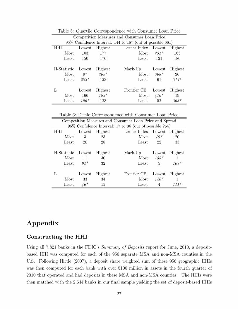
Table 5: Quartile Correspondence with Consumer Loan Price

Competition Measures and Consumer Loan Price95% Confidence Interval: 144 to 187 (out of possible 661)

HHI Lowest Highest Lerner Index Lowest HighestMost 103 177 Most 231* 163Least 150 176 Least 121 180

H-Statistic Lowest Highest Mark-Up Lowest HighestMost 97 205* Most 368* 26Least 283* 123 Least 61 317*

L Lowest Highest Frontier CE Lowest HighestMost 166 193* Most 416* 19Least 196* 123 Least 52 363*

Table 6: Decile Correspondence with Consumer Loan Price

Competition Measures and Consumer Loan Price and Spread95% Confidence Interval: 17 to 36 (out of possible 264)

HHI Lowest Highest Lerner Index Lowest HighestMost 3 23 Most 49* 20Least 20 28 Least 22 33

H-Statistic Lowest Highest Mark-Up Lowest HighestMost 11 30 Most 133* 1Least 94* 32 Least 5 107*

L Lowest Highest Frontier CE Lowest HighestMost 33 34 Most 146* 1Least 46* 15 Least 4 111*

Appendix

Constructing the HHI

Using all 7,821 banks in the FDIC’s Summary of Deposits report for June, 2010, a deposit-

based HHI was computed for each of the 956 separate MSA and non-MSA counties in the

U.S. Following Hirtle (2007), a deposit share weighted sum of these 956 geographic HHIs

was then computed for each bank with over $100 million in assets in the fourth quarter of

2010 that operated and had deposits in these MSA and non-MSA counties. The HHIs were

then matched with the 2,644 banks in our final sample yielding the set of deposit-based HHIs

27

50 100 150 200 250 300

0.05

0.10

0.15

0.20

0.25

0.30

Top Line: Price of Consumer Loans

Bottom Line: Price of Labor/5000

Figure 2: Relation Between Output Price and Scaled Price of Labor Input (first quarter, 2008)

Bank Asset Value

Interest Rate

Figure 2: Relation Between Output Price and Scaled Price of Labor Input (Billion DollarBanks)

used here. The very largest banks have foreign offices but the Summary of Deposits only has

information on domestic U.S. bank branch deposits and so our calculated HHIs apply only to

domestic U.S. market concentration.27

Computing the Mark-Up

It is not possible to estimate a Lerner Index directly for consumer loans using a cost function.

This is because the allocation of operating costs (labor, physical capital, and other non-interest

expense) to consumer loans is not reported. However, it is possible to determine the markup

of the average price of consumer loans (PCLOAN) over the likely interest rate of total deposit

and other funding expenses (PDEP ). This mark-up measure is determined from MARK-

UP = (PCLOAN − PDEP )/PCLOAN . As shown below, this is similar to the dependent

variable for the frontier CE estimation: (PCLOAN −PDEP )/OC, which is one reason why

MARK-UP is correlated with the frontier measure of competition in the text (R2 = .15). If

operating costs were allocated to the consumer loan function, it would have been possible to

compute a Lerner Index for just consumer loans.

27Summary of Deposits data are only available once a year in June. We chose to use the HHI for 2010 since,for a few of the very largest banks, their deposit market concentration would be somewhat higher due recentmergers/acquisitions. For billion dollar banks, the R2 between HHI values computed for 2010 (the year weused) and 2009 and 2008 are .85 and .87, respectively. Between 2008 and 2009 it was .94. Even so, only 2banks out of 382 flip consecutive places for consecutive years when all banks are ranked by their asset value.Using any or all of these years would unlikely have altered our results when comparing the HHI with the othercompetition measures.

28

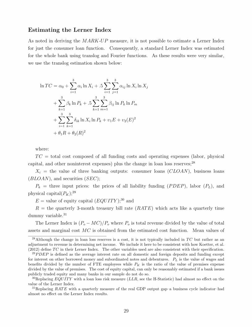
Estimating the Lerner Index

As noted in deriving the MARK-UP measure, it is not possible to estimate a Lerner Index

for just the consumer loan function. Consequently, a standard Lerner Index was estimated

for the whole bank using translog and Fourier functions. As these results were very similar,

we use the translog estimation shown below:

lnTC = α0 +3∑

i=1

αi lnXi + .53∑

i=1

3∑j=1

αij lnXi lnXj

+3∑

k=1

βk lnPk + .53∑

k=1

3∑m=1

βij lnPk lnPm

+3∑

i=1

3∑k=1

δik lnXi lnPk + υ1E + υ2(E)2

+ θ1R + θ2(R)2

where:

TC = total cost composed of all funding costs and operating expenses (labor, physical

capital, and other noninterest expenses) plus the change in loan loss reserves;28

Xi = the value of three banking outputs: consumer loans (CLOAN), business loans

(BLOAN), and securities (SEC);

Pk = three input prices: the prices of all liability funding (PDEP ), labor (PL), and

physical capital(PK);29

E = value of equity capital (EQUITY );30 and

R = the quarterly 3-month treasury bill rate (RATE) which acts like a quarterly time

dummy variable.31

The Lerner Index is (Po −MC)/Po where Po is total revenue divided by the value of total

assets and marginal cost MC is obtained from the estimated cost function. Mean values of

28Although the change in loan loss reserves is a cost, it is not typically included in TC but rather as anadjustment to revenue in determining net income. We include it here to be consistent with how Koetter, et al.(2012) define TC in their Lerner Index. The other variables used are also consistent with their specification.

29PDEP is defined as the average interest rate on all domestic and foreign deposits and funding exceptfor interest on other borrowed money and subordinated notes and debentures. PL is the value of wages andbenefits divided by the number of FTE employees while PK is the ratio of the value of premises expensedivided by the value of premises. The cost of equity capital, can only be reasonably estimated if a bank issuespublicly traded equity and many banks in our sample do not do so.

30Replacing EQUITY with a loan loss risk measure (LLR, see the H-Statistic) had almost no effect on thevalue of the Lerner Index.

31Replacing RATE with a quarterly measure of the real GDP output gap–a business cycle indicator–hadalmost no effect on the Lerner Index results.

29

the variables used to estimate all competition indicators except the HHI are shown in Table

A1 below. The entire panel was estimated as a single equation using OLSQ.

Estimating L, an Adjusted Lerner Index

A Lerner Index for the whole bank is adjusted for cost and profit inefficiency in Koetter,

Kolari, and Spierdijk (2012). Effectively, the adjustment substitutes an “efficiency corrected”

price (P ∗o ) for the observed price (Po) in a standard Lerner Index giving (P ∗

o − MC)/P ∗o .

Observed price would be computed using observed total cost (TC)32 and profits before taxes

(PBT ) in the Koetter, et al. (2012), model while we use net income (PFT ) as our profit

measure.33 Both TC and PFT are divided by the total value of the sum of specified outputs

(TO). As our cost function specification is identical to that above for the Lerner Index,

TO = CLOAN + BLOAN + SEC.34 Observed price in the Koetter, et al. (2012) model

appears to be Po = TC/TO+PFT/TO while the efficiency corrected price is P ∗o = TC∗/TO+

PFT ∗/TO. Efficiency corrected prices are based on the predicted values of TC and PFT from

the same translog cost specification used above for the Lerner Index and a separately estimated

alternative profit function. A Stochastic Frontier Approach (SFA) is used in estimation so

the residuals of the cost and profit estimations reflect both normal error and an assumed

half-normal distribution of cost or alternative profit inefficiency.35 The predicted values of

TC∗ and PFT ∗ are thus presumed to be reduced by the amount of SFA cost and profit

inefficiency. Importantly, an alternative profit function is used which reflects the opposite of

perfect competition–namely that banks have (monopoly) pricing power. Just as TC − TC∗

reflects the apparent deviation from minimum cost (due to cost inefficiency), PFT − PFT ∗

reflects the deviation from maximum profits when a bank has pricing power. Our adjusted

Lerner Index (L) follows the specification outlined in Koetter, et al. (2012) for their cost

function (their equation 4), changing only the dependent variable from TC in the cost function

to PFT for the alternative profit function.36 To estimate L it is necessary to consult the

32Koetter, et al. (2012) call this total operating cost but it is actually total cost since it includes the sum ofthe cost of labor, physical capital, and other non-interest expense (operating cost) plus all interest or fundingcost.

33Net income is more commonly referred to as profits in the banking industry while profits before taxesabstracts from tax effects. As noted for the Lerner Index, TC includes the change in the provision for loanlosses as part of costs.

34In their estimation, Koetter, et al. (2012), specify two outputs: TO = total loans (the sum of CLOANand BLOAN) and SEC. Total assets (TA) are, on average, 37% larger larger than total output (TO) in oursample.

35If the SFA assumption of a half-normal distribution of inefficiency is deemed problematic, the DistributionFree Approach (DFA) to frontier efficiency measurement can be used instead. With DFA, the predictedvalues of TC∗ and PFT ∗ can be obtained with multiple quarterly OLSQ cross-section estimation alone as theseparation of inefficiency from normal error in the composed error residual occurs later.

36The average fit of the cost function was R2 = .97 and .89 for the alternative profit function used to computeL2 with OLSQ. No R2 is available for L since it is estimated using SFA.

30

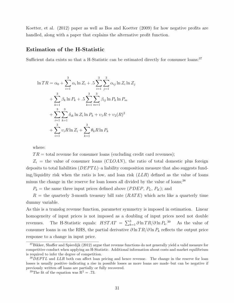
Koetter, et al. (2012) paper as well as Bos and Koetter (2009) for how negative profits are

handled, along with a paper that explains the alternative profit function.

Estimation of the H-Statistic

Sufficient data exists so that a H-Statistic can be estimated directly for consumer loans:37

lnTR = α0 +3∑

i=1

αi lnZi + .53∑

i=1

3∑j=1

αij lnZi lnZj

+3∑

k=1

βk lnPk + .53∑

k=1

3∑m=1

βij lnPk lnPm

+3∑

i=1

3∑k=1

δik lnZi lnPk + υ1R + υ2(R)2

+3∑

i=1

υiR lnZi +3∑

k=1

θkR lnPk

where:

TR = total revenue for consumer loans (excluding credit card revenues);

Zi = the value of consumer loans (CLOAN), the ratio of total domestic plus foreign

deposits to total liabilities (DEPTL)–a liability composition measure that also suggests fund-

ing/liquidity risk when the ratio is low, and loan risk (LLR) defined as the value of loans

minus the change in the reserve for loan losses all divided by the value of loans;38

Pk = the same three input prices defined above (PDEP , PL, PK); and

R = the quarterly 3-month treasury bill rate (RATE) which acts like a quarterly time

dummy variable.

As this is a translog revenue function, parameter symmetry is imposed in estimation. Linear

homogeneity of input prices is not imposed as a doubling of input prices need not double

revenues. The H-Statistic equals: HSTAT =∑3

k=1 ∂ lnTR/∂ lnPk.39 As the value of

consumer loans is on the RHS, the partial derivative ∂ lnTR/∂ lnPk reflects the output price

response to a change in input price.

37Bikker, Shaffer and Spierdijk (2012) argue that revenue functions do not generally yield a valid measure forcompetitive conduct when applying an H-Statistic. Additional information about costs and market equilibriumis required to infer the degree of competition.

38DEPTL and LLR both can affect loan pricing and hence revenue. The change in the reserve for loanlosses is usually positive–indicating a rise in possible losses as more loans are made–but can be negative ifpreviously written off loans are partially or fully recovered.

39The fit of the equation was R2 = .73.

31

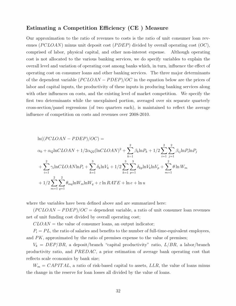
Estimating a Competition Efficiency (CE ) Measure

Our approximation to the ratio of revenues to costs is the ratio of unit consumer loan rev-

enues (PCLOAN) minus unit deposit cost (PDEP ) divided by overall operating cost (OC),

comprised of labor, physical capital, and other non-interest expense. Although operating

cost is not allocated to the various banking services, we do specify variables to explain the

overall level and variation of operating cost among banks which, in turn, influence the effect of

operating cost on consumer loans and other banking services. The three major determinants

of the dependent variable (PCLOAN − PDEP )/OC in the equation below are the prices of

labor and capital inputs, the productivity of these inputs in producing banking services along

with other influences on costs, and the existing level of market competition. We specify the

first two determinants while the unexplained portion, averaged over six separate quarterly

cross-section/panel regressions (of two quarters each), is maintained to reflect the average

influence of competition on costs and revenues over 2008-2010.

ln((PCLOAN − PDEP )/OC) =

α0 + αQlnCLOAN + 1/2αQ2(lnCLOAN)2 +2∑

k=1

βklnPk + 1/22∑

i=1

2∑j=1

βijlnPilnPj

+2∑

i=1

γilnCLOAN lnPi +3∑

k=1

δklnVk + 1/23∑

k=1

3∑p=1

δkplnVklnVp +2∑

m=1

θ lnWm

+ 1/22∑

m=1

2∑q=1

θmqlnWmlnWq + ε lnRATE + ln e+ lnu

where the variables have been defined above and are summarized here:

(PCLOAN − PDEP )/OC = dependent variable, a ratio of unit consumer loan revenues

net of unit funding cost divided by overall operating cost;

CLOAN = the value of consumer loans, an output indicator;

Pi = PL, the ratio of salaries and benefits to the number of full-time-equivalent employees,

and PK, approximated by the ratio of premises expense to the value of premises;

Vk = DEP/BR, a deposit/branch “capital productivity” ratio, L/BR, a labor/branch

productivity ratio, and PREDAC, a prior estimation of average bank operating cost that

reflects scale economics by bank size;

Wm = CAPITAL, a ratio of risk-based capital to assets, LLR, the value of loans minus

the change in the reserve for loan losses all divided by the value of loans.

32

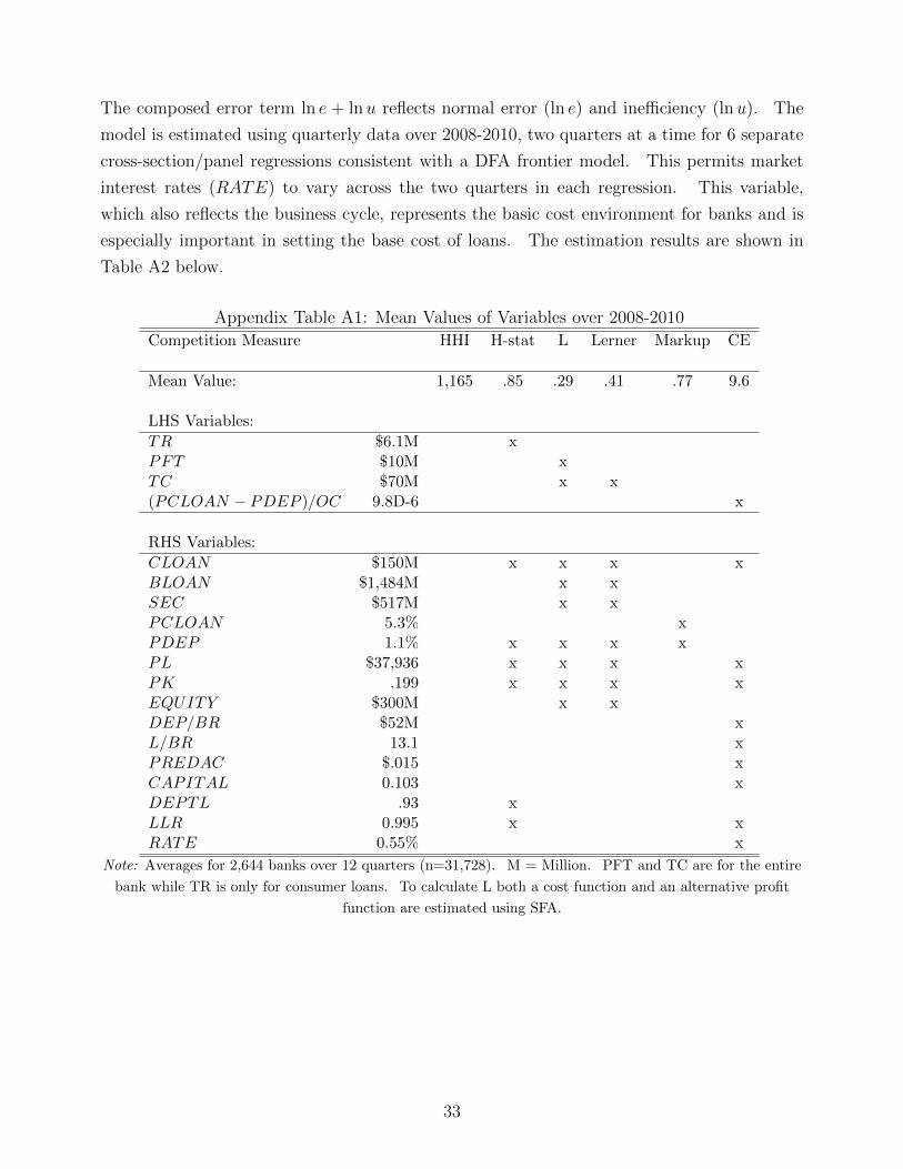
The composed error term ln e + lnu reflects normal error (ln e) and inefficiency (lnu). The

model is estimated using quarterly data over 2008-2010, two quarters at a time for 6 separate

cross-section/panel regressions consistent with a DFA frontier model. This permits market

interest rates (RATE) to vary across the two quarters in each regression. This variable,

which also reflects the business cycle, represents the basic cost environment for banks and is

especially important in setting the base cost of loans. The estimation results are shown in

Table A2 below.

Appendix Table A1: Mean Values of Variables over 2008-2010

Competition Measure HHI H-stat L Lerner Markup CE

Mean Value: 1,165 .85 .29 .41 .77 9.6

LHS Variables:

TR $6.1M xPFT $10M xTC $70M x x(PCLOAN − PDEP )/OC 9.8D-6 x

RHS Variables:

CLOAN $150M x x x xBLOAN $1,484M x xSEC $517M x xPCLOAN 5.3% xPDEP 1.1% x x x xPL $37,936 x x x xPK .199 x x x xEQUITY $300M x xDEP/BR $52M xL/BR 13.1 xPREDAC $.015 xCAPITAL 0.103 xDEPTL .93 xLLR 0.995 x xRATE 0.55% x

Note: Averages for 2,644 banks over 12 quarters (n=31,728). M = Million. PFT and TC are for the entire

bank while TR is only for consumer loans. To calculate L both a cost function and an alternative profit

function are estimated using SFA.

33

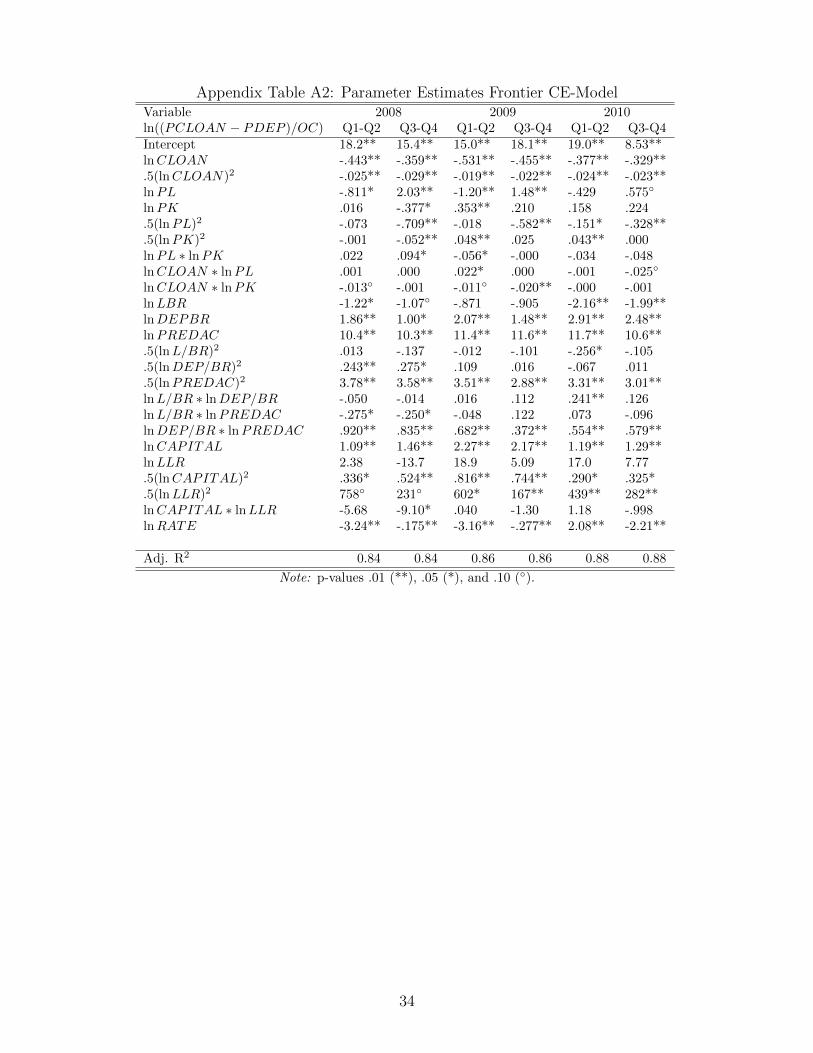
Appendix Table A2: Parameter Estimates Frontier CE-ModelVariable 2008 2009 2010ln((PCLOAN − PDEP )/OC) Q1-Q2 Q3-Q4 Q1-Q2 Q3-Q4 Q1-Q2 Q3-Q4Intercept 18.2** 15.4** 15.0** 18.1** 19.0** 8.53**lnCLOAN -.443** -.359** -.531** -.455** -.377** -.329**.5(lnCLOAN)2 -.025** -.029** -.019** -.022** -.024** -.023**lnPL -.811* 2.03** -1.20** 1.48** -.429 .575◦

lnPK .016 -.377* .353** .210 .158 .224.5(lnPL)2 -.073 -.709** -.018 -.582** -.151* -.328**.5(lnPK)2 -.001 -.052** .048** .025 .043** .000lnPL ∗ lnPK .022 .094* -.056* -.000 -.034 -.048lnCLOAN ∗ lnPL .001 .000 .022* .000 -.001 -.025◦

lnCLOAN ∗ lnPK -.013◦ -.001 -.011◦ -.020** -.000 -.001lnLBR -1.22* -1.07◦ -.871 -.905 -2.16** -1.99**lnDEPBR 1.86** 1.00* 2.07** 1.48** 2.91** 2.48**lnPREDAC 10.4** 10.3** 11.4** 11.6** 11.7** 10.6**.5(lnL/BR)2 .013 -.137 -.012 -.101 -.256* -.105.5(lnDEP/BR)2 .243** .275* .109 .016 -.067 .011.5(lnPREDAC)2 3.78** 3.58** 3.51** 2.88** 3.31** 3.01**lnL/BR ∗ lnDEP/BR -.050 -.014 .016 .112 .241** .126lnL/BR ∗ lnPREDAC -.275* -.250* -.048 .122 .073 -.096lnDEP/BR ∗ lnPREDAC .920** .835** .682** .372** .554** .579**lnCAPITAL 1.09** 1.46** 2.27** 2.17** 1.19** 1.29**lnLLR 2.38 -13.7 18.9 5.09 17.0 7.77.5(lnCAPITAL)2 .336* .524** .816** .744** .290* .325*.5(lnLLR)2 758◦ 231◦ 602* 167** 439** 282**lnCAPITAL ∗ lnLLR -5.68 -9.10* .040 -1.30 1.18 -.998lnRATE -3.24** -.175** -3.16** -.277** 2.08** -2.21**

Adj. R2 0.84 0.84 0.86 0.86 0.88 0.88

Note: p-values .01 (**), .05 (*), and .10 (◦).

34

Previous DNB Working Papers in 2015 No. 454 Mauro Mastrogiacomo and Rob Alessie, Where are the retirement savings of self-

employed? An analysis of ‘unconventional’ retirement accounts No. 455 Clemens Bonner and Paul Hilbers, Global liquidity regulation - Why did it take so long? No. 456 Leo de Haan, Jan Willem van den End and Philip Vermeulen, Lenders on the storm of

wholesale funding shocks: Saved by the central bank?