dm 04 03 bayesian...

Data MiningPart 4. Prediction

4.3. Bayesian Classification

Bayesian Classification

Fall 2009

Instructor: Dr. Masoud Yaghini

Outline

� Introduction

� Bayes’ Theorem

� Naïve Bayesian Classification

� References


Introduction


Introduction

� Bayesian classifiers – A statistical classifiers

– performs probabilistic prediction, i.e., predicts class membership probabilities, such as the probability that a given instance belongs to a particular class.

� Foundation


Foundation– Based on Bayes’ Theorem.

� Performance– A simple Bayesian classifier, naïve Bayesian classifier, has

comparable performance with decision tree and selected neural network classifiers

– have also exhibited high accuracy and speed when applied to large databases.

Introduction

� Incremental

– Each training example can incrementally increase/decrease the probability that a hypothesis is correct

� Popular methods

– Naïve Bayesian classifier


– Naïve Bayesian classifier

– Bayesian belief networks

Introduction

� Naïve Bayesian classifier

– Naïve Bayesian classifiers assume that the effect of an attribute value on a given class is independent of the values of the other attributes.

– This assumption is called class conditional independence.


independence.

– It is made to simplify the computations involved and, in this sense, is considered “naïve.”

– Naïve Bayesian classifier, has comparable performance with decision tree and selected neural network classifiers

Introduction

� Bayesian belief networks

– Bayesian belief networks are graphical models, which unlike naïve Bayesian classifiers, allow the representation of dependencies among subsets of attributes.

– Bayesian belief networks can also be used for


– Bayesian belief networks can also be used for classification.

Bayes’ Theorem


Bayes’ Theorem

� Let :

– X: be a data sample: class label is unknown

– H: a hypothesis that X belongs to class C

– P(H | X) (Determined by classifier)

� The probability that instance X belongs to class C


The probability that instance X belongs to class C

� We know the attribute description of X.

– P(H): The probability of H

– P(X): The probability that sample data is observed

– P(X | H) is the probability of X conditioned on H.

Bayes’ Theorem

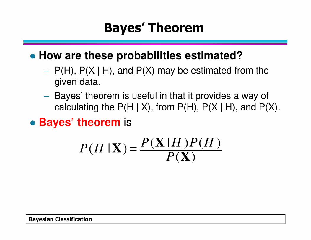
� How are these probabilities estimated?

– P(H), P(X | H), and P(X) may be estimated from the given data.

– Bayes’ theorem is useful in that it provides a way of calculating the P(H | X), from P(H), P(X | H), and P(X).

� Bayes’ theorem is


� Bayes’ theorem is

)(

)()|()|(

X

XX

PHPHPHP =

Bayes’ Theorem

� Example:

– Suppose customers described by the attributes age and income

– X: a 35-year-old customer with an income of $40,000.

– H: the hypothesis that the customer will buy a computer.


computer.

– P(H | X): the probability that customer X will buy a computer given that we know the customer’s age and income.

– P(H): the probability that any given customer will buy a computer, regardless of age and income

Bayes’ Theorem

� Example: (cont.)

– P(X): the probability that a person from our set of customers is 35 years old and earns $40,000.

– P(X | H): the probability that a customer, X, is 35 years old and earns $40,000, given that we know the customer will buy a computer.


customer will buy a computer.

Bayes’ Theorem

� Practical difficulty

– require initial knowledge of many probabilities, significant computational cost

� Now that we’ve got that out of the way, in the next section, we will look at how Bayes’ theorem


next section, we will look at how Bayes’ theorem is used in the naive Bayesian classifier.

Naïve Bayesian Classification



� Naïve bayes classifier use all the attributes

� Two assumptions:

– Attributes are equally important

– Attributes are statistically independent

� I.e., knowing the value of one attribute says nothing about the value of another


value of another

� Equally important & independence assumptions are never correct in real-life datasets


� The naïve Bayesian classifier works as follows:

1. Let D be a training set of instances and their associated class labels,

– each instance is represented by an n-dimentionalattribute vector X = (x1, x2, …, xn)


2. Suppose there are m classes C1, C2, …, Cm.

– The classifier will predict that X belongs to the class Ci if and only if:


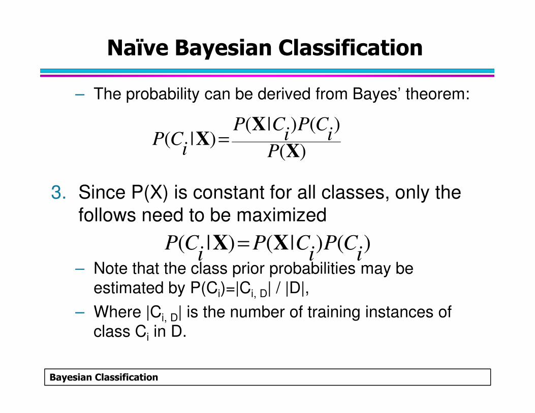
– The probability can be derived from Bayes’ theorem:

3. Since P(X) is constant for all classes, only the follows need to be maximized

)(

)()|()|(

X

XX

Pi

CPi

CP

iCP =


follows need to be maximized

– Note that the class prior probabilities may be estimated by P(Ci)=|Ci, D| / |D|,

– Where |Ci, D| is the number of training instances of class Ci in D.

)()|()|(i

CPi

CPi

CP XX =


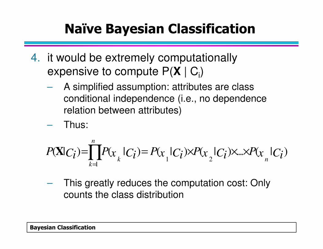
4. it would be extremely computationally expensive to compute P(X | Ci)

– A simplified assumption: attributes are class conditional independence (i.e., no dependence relation between attributes)

– Thus:


– Thus:

– This greatly reduces the computation cost: Only counts the class distribution

1 21

( | ) ( | ) ( | ) ( | ) ... ( | )n

k nk

P P P P PC C C C Cx x x xi i i i i=

= = × × ×∏X


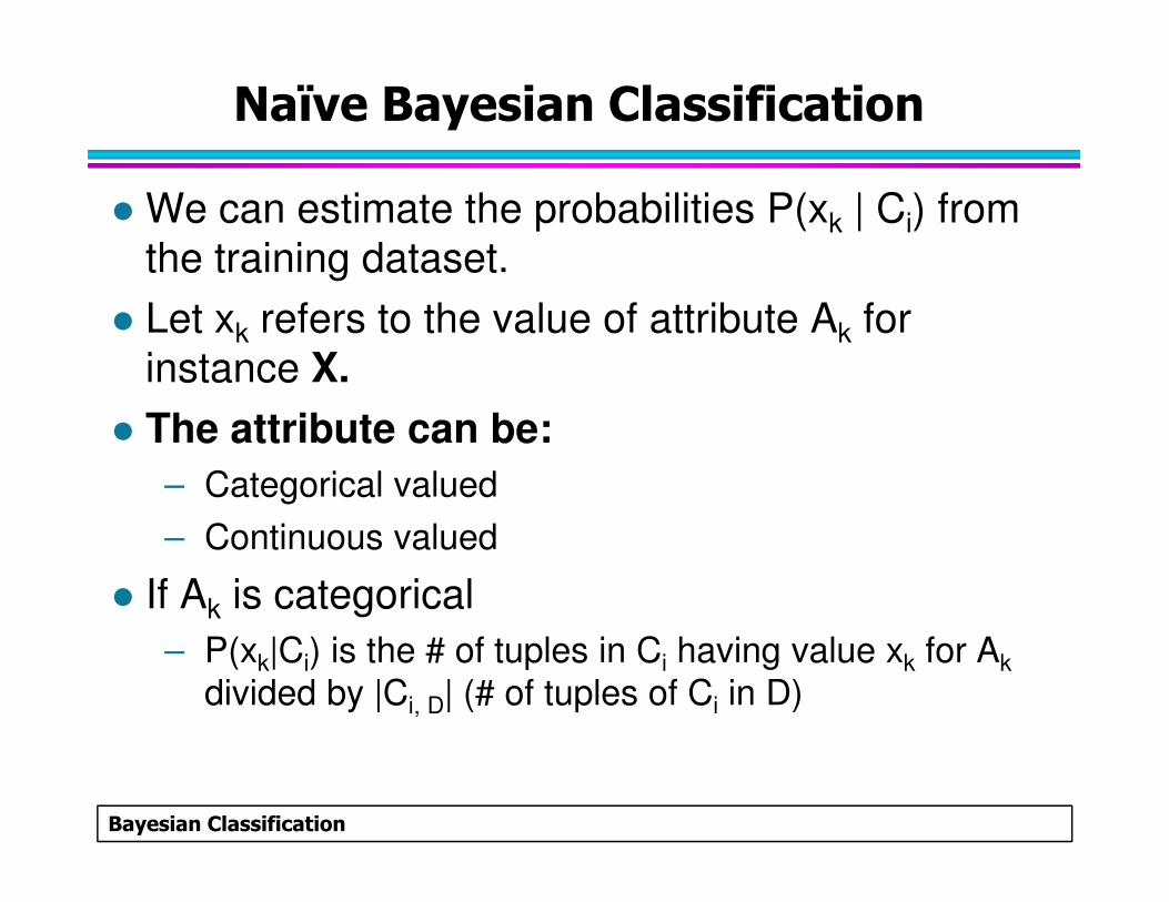
� We can estimate the probabilities P(xk | Ci) from the training dataset.

� Let xk refers to the value of attribute Ak for instance X.

� The attribute can be:


– Categorical valued

– Continuous valued

� If Ak is categorical

– P(xk|Ci) is the # of tuples in Ci having value xk for Ak

divided by |Ci, D| (# of tuples of Ci in D)


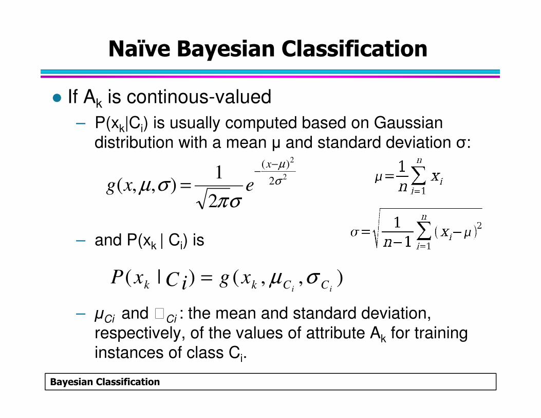
� If Ak is continous-valued

– P(xk|Ci) is usually computed based on Gaussian distribution with a mean µ and standard deviation σ:

2

2

2

)(

2

1),,( σ

µ

σπσµ

−−

=x

exg


– and P(xk | Ci) is

– µCi and Ci : the mean and standard deviation, respectively, of the values of attribute Ak for training instances of class Ci.

2 σπ

),,()|(ii CCkk xgCixP σµ=


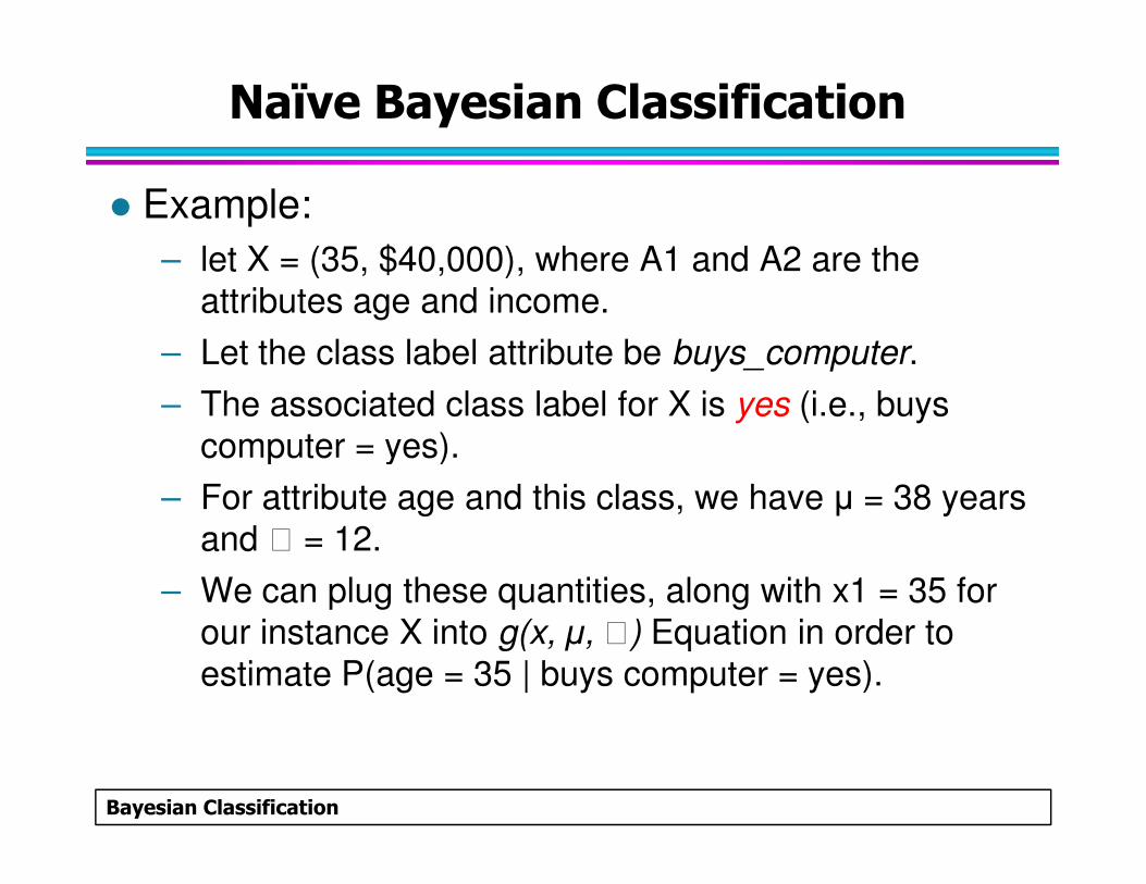
� Example:

– let X = (35, $40,000), where A1 and A2 are the attributes age and income.

– Let the class label attribute be buys_computer.

– The associated class label for X is yes (i.e., buys computer = yes).


computer = yes).

– For attribute age and this class, we have µ = 38 years and = 12.

– We can plug these quantities, along with x1 = 35 for our instance X into g(x, µ, ) Equation in order to estimate P(age = 35 | buys computer = yes).

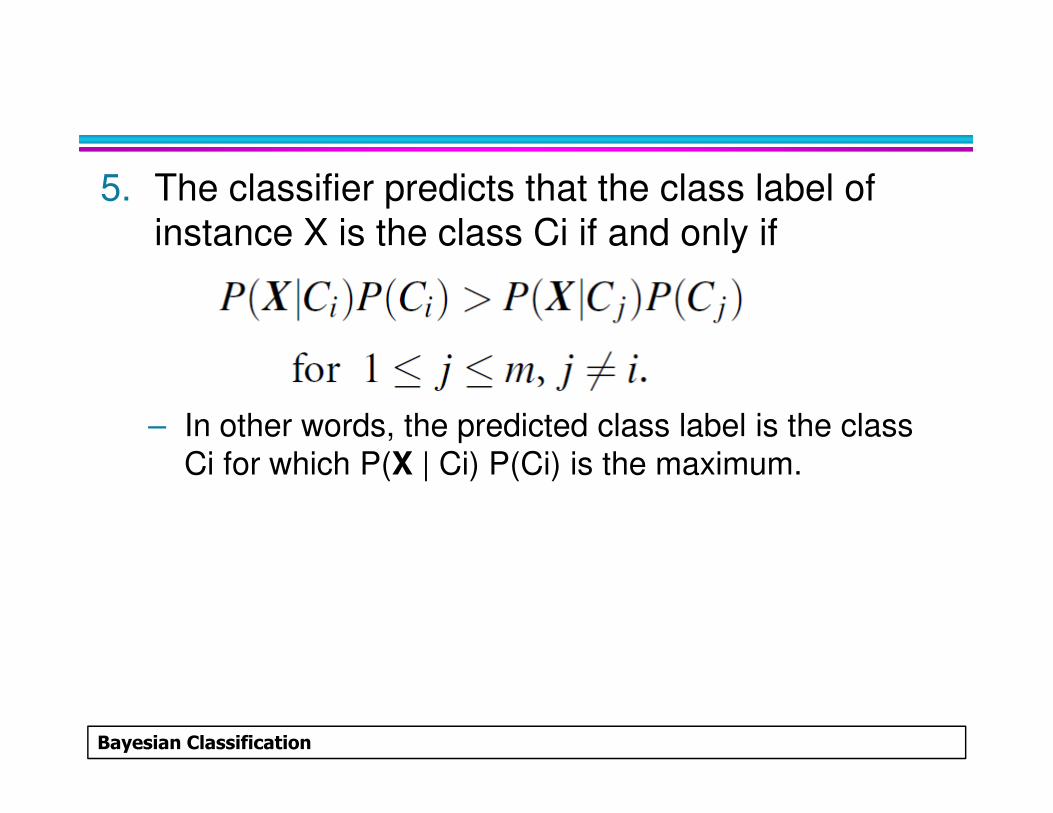
5. The classifier predicts that the class label of instance X is the class Ci if and only if


– In other words, the predicted class label is the class Ci for which P(X | Ci) P(Ci) is the maximum.

Example 1: AllElectronics


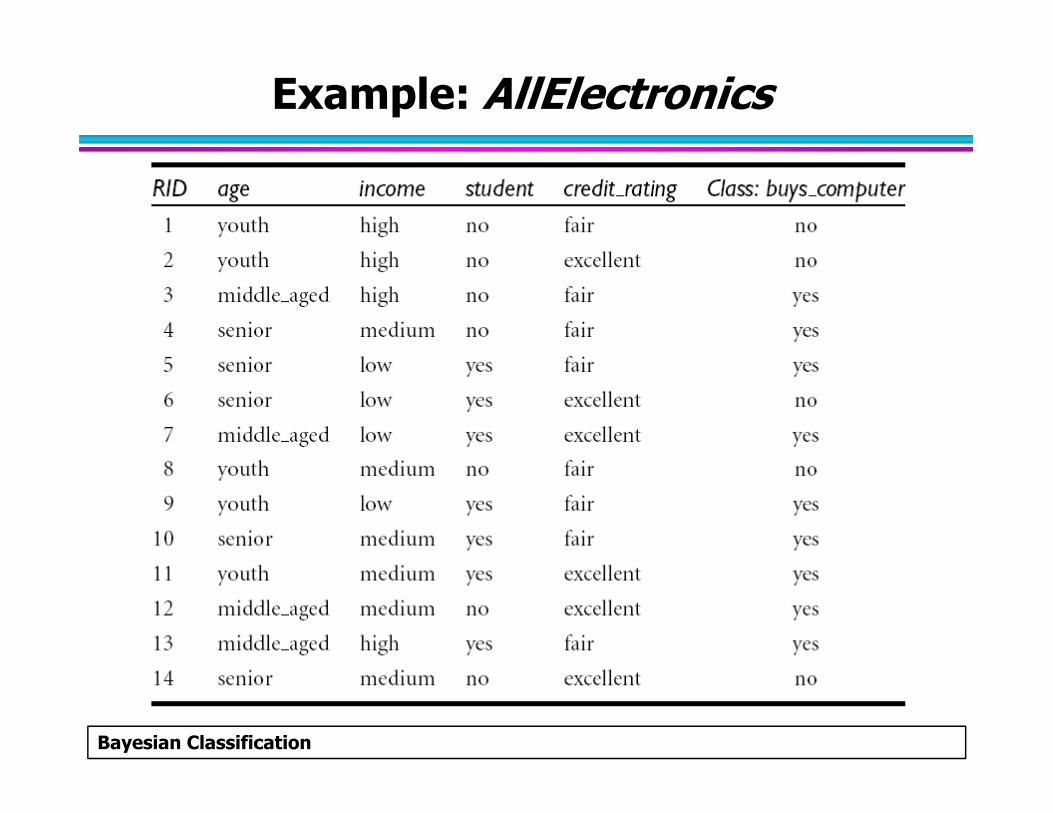
Example 1: AllElectronics

� We wish to predict the class label of a instance using naïve Bayesian classification given the AllElectronics training data

� The data instances are described by the attributes age, income, student, and credit rating.


� The class label attribute, buys _computer, has two distinct values

� Let

– C1 correspond to the class buys computer = yes

– C2 correspond to the class buys computer = no

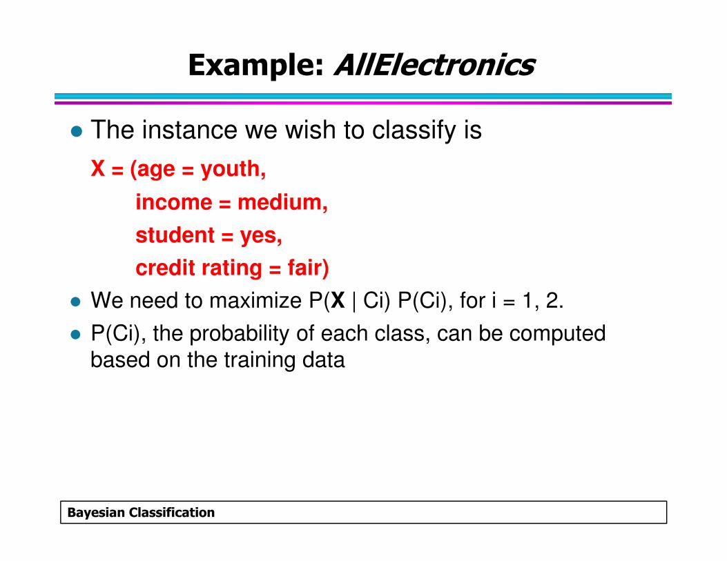
Example: AllElectronics



� The instance we wish to classify is

X = (age = youth,

income = medium,

student = yes,

credit rating = fair)


� We need to maximize P(X | Ci) P(Ci), for i = 1, 2.

� P(Ci), the probability of each class, can be computed based on the training data


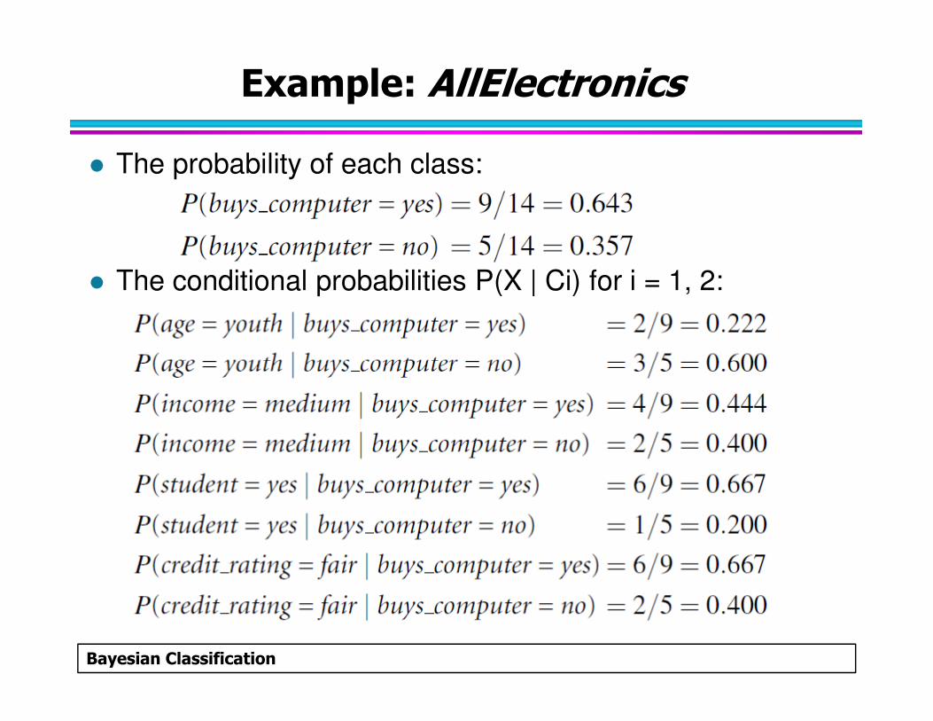
� The probability of each class:

� The conditional probabilities P(X | Ci) for i = 1, 2:



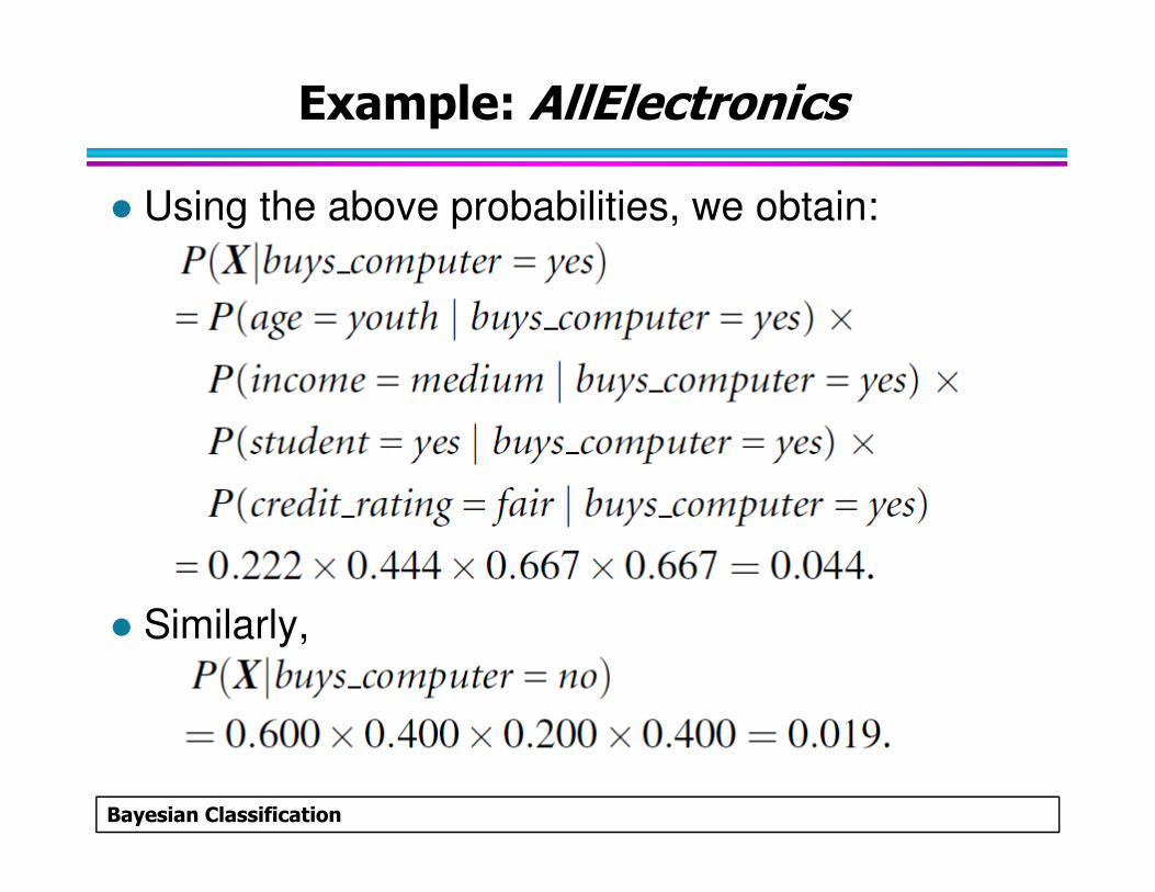
� Using the above probabilities, we obtain:


� Similarly,


� To find the class we compute P(X | Ci) P(Ci):


� Therefore, the naïve Bayesian classifier predicts buys computer = yes for instance X.

Avoiding the 0-Probability Problem

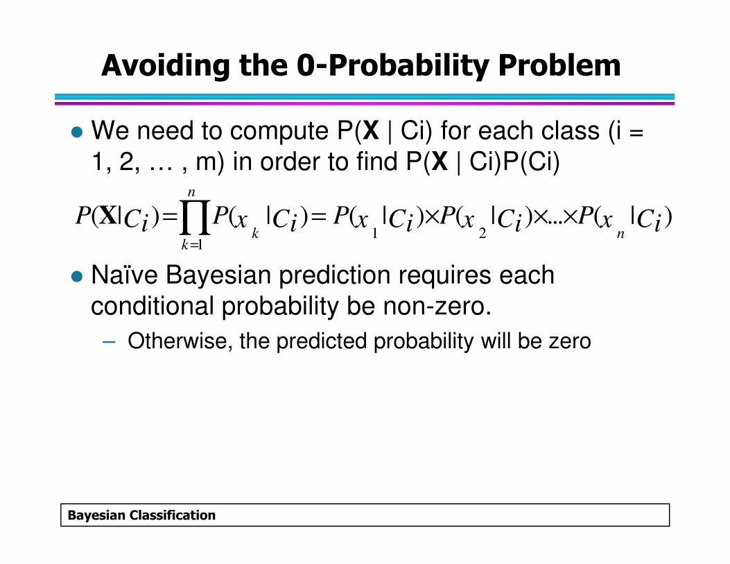
� We need to compute P(X | Ci) for each class (i = 1, 2, … , m) in order to find P(X | Ci)P(Ci)

� Naïve Bayesian prediction requires each

1 21

( | ) ( | ) ( | ) ( | ) ... ( | )n

k nk

P P P P PC C C C Cx x x xi i i i i=

= = × × ×∏X


� Naïve Bayesian prediction requires each conditional probability be non-zero.

– Otherwise, the predicted probability will be zero


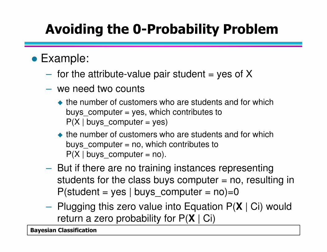
� Example:

– for the attribute-value pair student = yes of X

– we need two counts

� the number of customers who are students and for which buys_computer = yes, which contributes to P(X | buys_computer = yes)


P(X | buys_computer = yes)

� the number of customers who are students and for which buys_computer = no, which contributes to P(X | buys_computer = no).

– But if there are no training instances representing students for the class buys computer = no, resulting in P(student = yes | buys_computer = no)=0

– Plugging this zero value into Equation P(X | Ci) would return a zero probability for P(X | Ci)


� Laplacian correction (Laplacian estimator)

– We assume that our training database, D, is so large

– Adding 1 to each case

– It makes a negligible difference in the estimated probability value

– It would conveniently avoid the case of probability


– It would conveniently avoid the case of probability values of zero.


� Use Laplacian correction (or Laplacianestimator)

– Adding 1 to each case

� Prob(income = low) = 1/1003

� Prob(income = medium) = 991/1003

� Prob(income = high) = 11/1003


� Prob(income = high) = 11/1003

– The “corrected” prob. estimates are close to their “uncorrected” counterparts


� Example:

– Suppose that for the class buys_computer = yes in training database, D, containing 1,000 instances

– We have

� 0 instances with income = low,

� 990 instances with income = medium, and


� 990 instances with income = medium, and

� 10 instances with income = high.

– The probabilities of these events are 0 (from 0/1000), 0.990 (from 999/1000), and 0.010 (from 10/1,000)

– Using the Laplacian correction for the three quantities, we pretend that we have 1 more instance for each income-value pair.


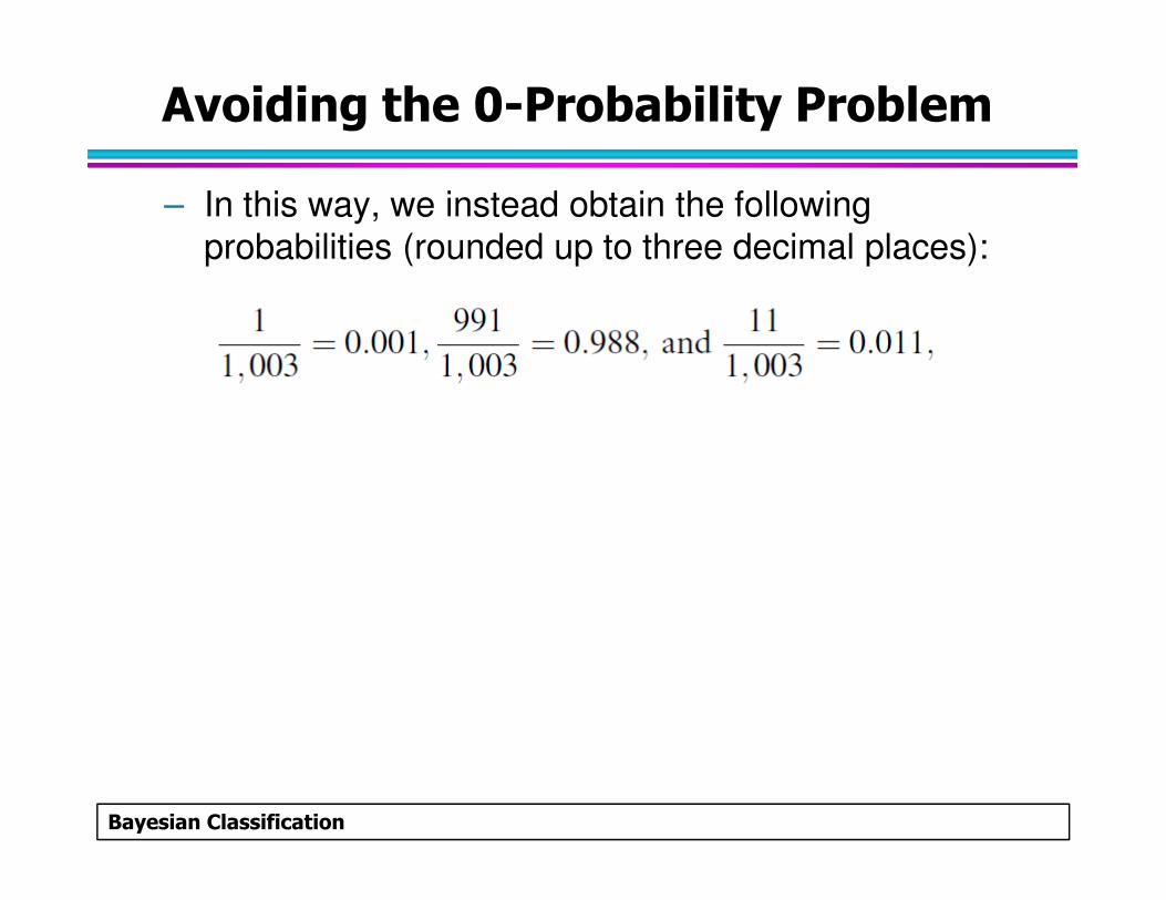
– In this way, we instead obtain the following probabilities (rounded up to three decimal places):


Example 2: Weather Problem


Weather Problem


Weather Problem


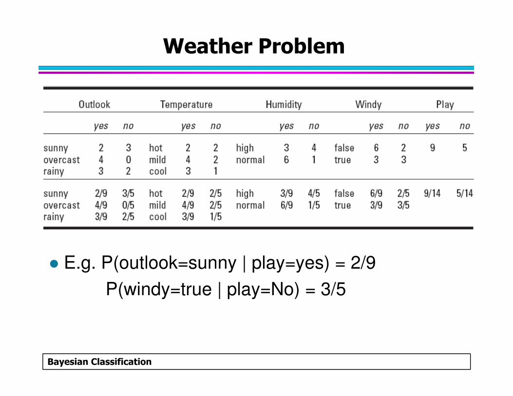
� E.g. P(outlook=sunny | play=yes) = 2/9

P(windy=true | play=No) = 3/5

Probabilities for weather data

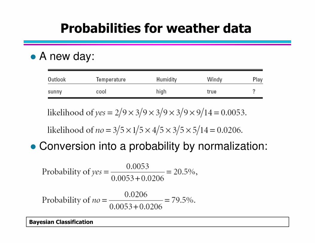
� A new day:


� Conversion into a probability by normalization:

Bayes’s rule

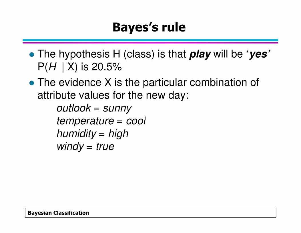
� The hypothesis H (class) is that play will be ‘yes’

P(H | X) is 20.5%

� The evidence X is the particular combination of attribute values for the new day:

outlook = sunny

temperature = cool


temperature = cool

humidity = high

windy = true

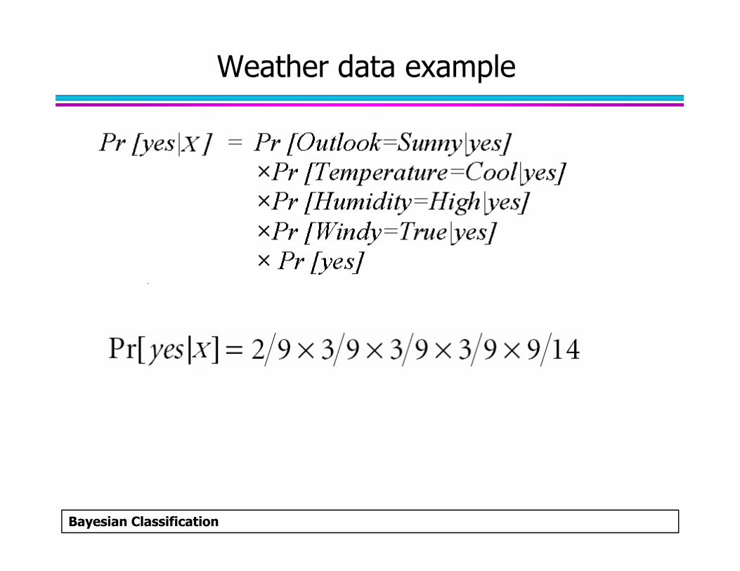
Weather data example


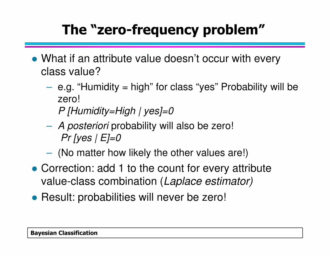
The “zero-frequency problem”

� What if an attribute value doesn’t occur with every class value?

– e.g. “Humidity = high” for class “yes” Probability will be zero! P [Humidity=High | yes]=0

– A posteriori probability will also be zero!


– A posteriori probability will also be zero!Pr [yes | E]=0

– (No matter how likely the other values are!)

� Correction: add 1 to the count for every attribute value-class combination (Laplace estimator)

� Result: probabilities will never be zero!

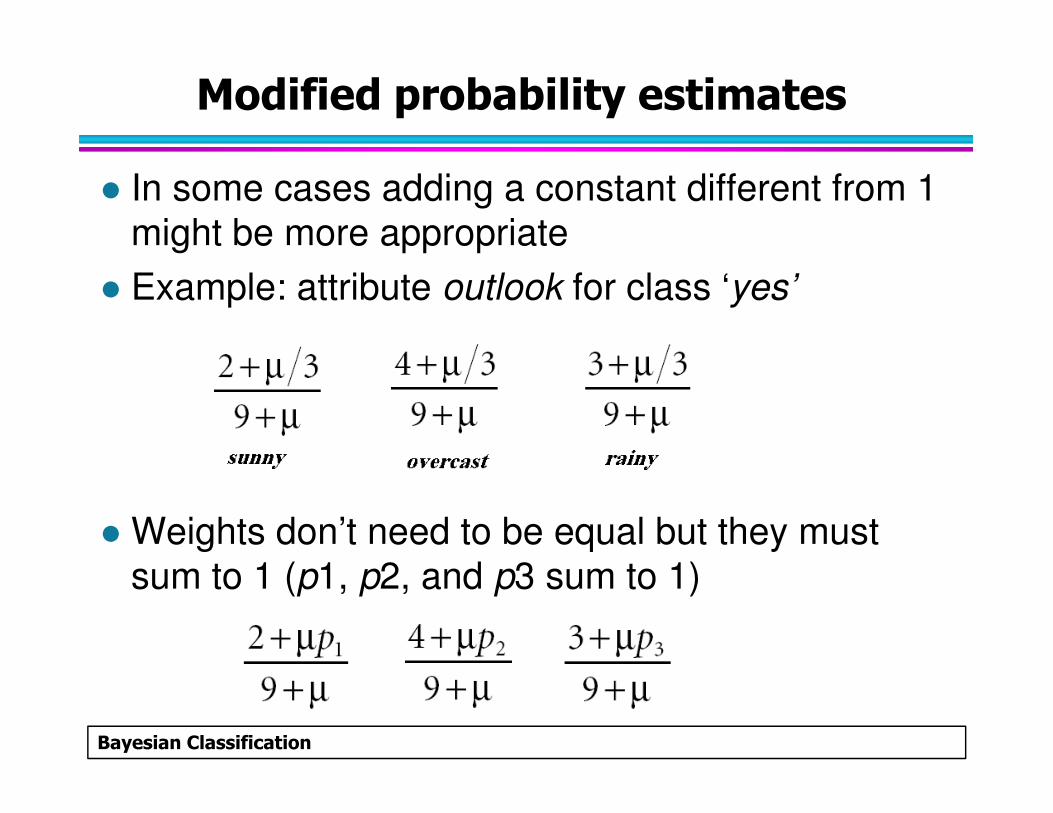
Modified probability estimates

� In some cases adding a constant different from 1 might be more appropriate

� Example: attribute outlook for class ‘yes’


� Weights don’t need to be equal but they must sum to 1 (p1, p2, and p3 sum to 1)

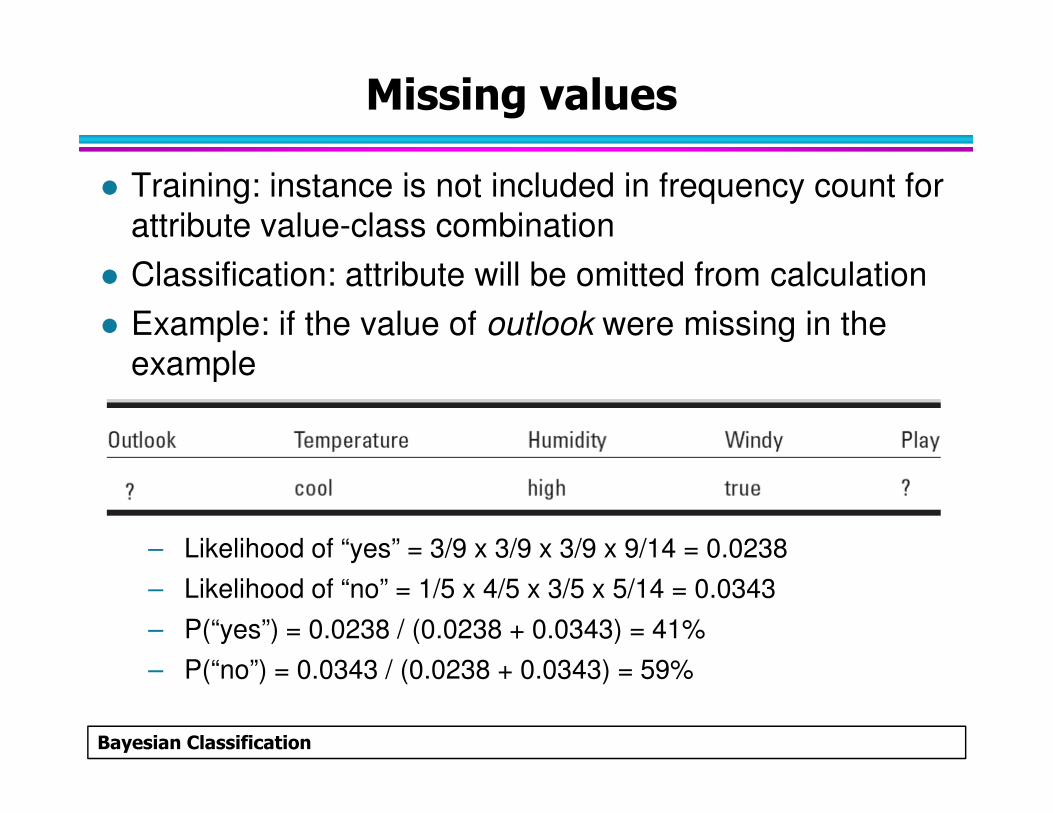
Missing values

� Training: instance is not included in frequency count for attribute value-class combination

� Classification: attribute will be omitted from calculation

� Example: if the value of outlook were missing in the example


– Likelihood of “yes” = 3/9 x 3/9 x 3/9 x 9/14 = 0.0238

– Likelihood of “no” = 1/5 x 4/5 x 3/5 x 5/14 = 0.0343

– P(“yes”) = 0.0238 / (0.0238 + 0.0343) = 41%

– P(“no”) = 0.0343 / (0.0238 + 0.0343) = 59%

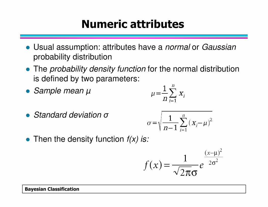
Numeric attributes

� Usual assumption: attributes have a normal or Gaussian probability distribution

� The probability density function for the normal distribution is defined by two parameters:

� Sample mean µ


� Standard deviation σ

� Then the density function f(x) is:

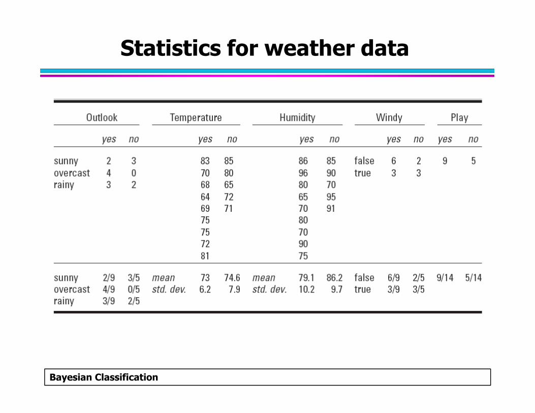
Statistics for weather data


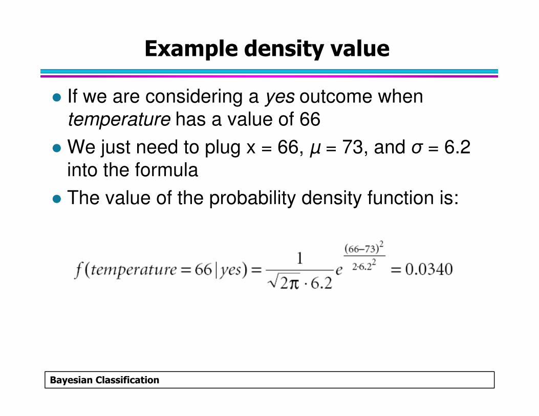
Example density value

� If we are considering a yes outcome when temperature has a value of 66

� We just need to plug x = 66, µ = 73, and σ = 6.2 into the formula

� The value of the probability density function is:


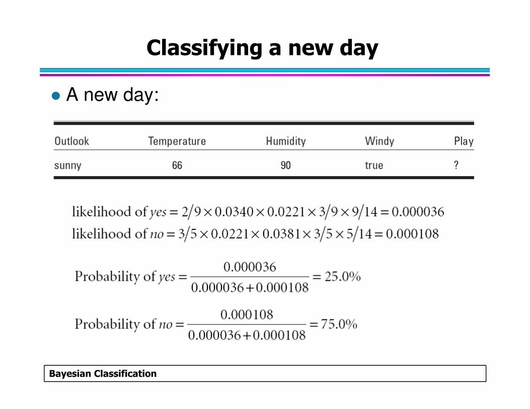
Classifying a new day

� A new day:


Comments


Missing values

� Missing values during training are not included in calculation of mean and standard deviation


Naïve Bayesian Classifier: Comments

� Advantages

– Easy to implement

– Good results obtained in most of the cases

� Disadvantages

– Assumption: class conditional independence, therefore loss of accuracy


therefore loss of accuracy

– Practically, dependencies exist among variables

� How to deal with these dependencies?

– Bayesian Belief Networks

References


References

� J. Han, M. Kamber, Data Mining: Concepts and Techniques, Elsevier Inc. (2006). (Chapter 6)

� I. H. Witten and E. Frank, Data Mining: Practical Machine Learning Tools and Techniques, 2nd Edition, Elsevier Inc., 2005. (Chapter 6)


The end


dm 04 03 bayesian...

Documents