Class Structure and Inequality during the Industrial Revolution: Lessons from England’s Social Tables,

1688-1867

Robert C. Allen

May 2017

Working Paper # 0002

Division of Social Science Working Paper Series

New York University Abu Dhabi, Saadiyat Island P.O Box 129188, Abu Dhabi, UAE

http://nyuad.nyu.edu/en/academics/academic-divisions/social-science.html

Class Structure and Inequality during the Industrial Revolution: Lessons from England’s Social Tables, 1688-1867

by

Robert C. Allen

Global Distinguished Professor of Economic History

Faculty of Social ScienceNew York University Abu Dhabi

Abu Dhabi, UAE

Senior Research FellowNuffield College, Oxford

email: bob.allen@nyu.edu

2017

Abstract

This paper measures the size and incomes of six major social classes across the IndustrialRevolution using social tables for England and Wales in 1688, 1759, 1798, 1846, and 1867. Lindert and Williamson famously revised these tables, and this paper extends their work inthree directions: First, servants are removed from middle and upper class households in thetables of King, Massie, and Colquhoun and tallied separately. Second, estimates are madefor the same tables of the number and incomes of women and children employed in thevarious occupations, and, third, incomes are broken down into rents, profits, and employmentincome. These extensions to the tables allow variables to be computed that can be checkedagainst independent estimates as a validation exercise. The tables are retabulated in astandardized set of six social groups to highlight the changing structure of society across theindustrial revolution. Gini coefficients are computed from the social tables to measureinequality. These measures confirm that Britain traversed a ‘Kuznets curve’ in this period. Changes in overall inequality are related to the changing fortunes of the major social classes.

keywords: social table, industrial revolution, national income, income distribution

JEL codes: N13, N33, N53

Measuring the changes in Britain’s economy and society over the course of theIndustrial Revolution has been a challenge for economists and historians for many decades. The most progress has been made in measuring the population and GDP1. Progress has beensubstantial but less definitive when it comes to tracking changes in the class structure, thedistribution of income and overall inequality.2 This paper revises and extends social tablesfor England to measure the sizes and incomes of the major social groups between 1688 and1867. These new tables embody answers to many questions including: How did the sizes ofthe upper, middle, and working classes change during the Industrial Revolution? Howprosperous was Britain before and during the Industrial Revolution and how far down thesocial hierarchy did that prosperity extend? Did all groups share in the growth of incomeduring the Industrial Revolution or were gains confined to only a few? Did British historytrace out a ‘Kuznetz curve’ of rising and then falling inequality during the IndustrialRevolution? And how was the history of overall inequality related to the shifting fortunes ofthe principal social classes?

Social tables are a tempting way to answer these questions. In a social table, societyis divided into status or occupational groups, and the numbers of households in each groupand their average incomes are specified.3 The first social table for England was drawn up byGregory King to show the state of the country in 1688.4 King’s table was well known anddefined the genre. Massie updated King’s work for 1759, Colquhoun revised it extensivelyto describe England as revealed by the first census in 1801, and Smee and Baxter madefurther revisions using the occupational data in the censuses of 1841 and 1861, as well asinformation from income tax returns.5 These tables present the historian with the tantalizingpossibility of comparing not only the average income of the country across the IndustrialRevolution, but also its distribution across social classes.

Well-known difficulties, however, stand in the way.6 The investigators had varyingsources of information, and some of it was unreliable, especially in the early tables. WhileKing’s population estimate was close to the mark, probably because he had access to thehearth tax returns and so had a reasonably correct idea of the number of inhabited houses, hisoccupational breakdown was very inaccurate. Massie had even less information to workwith. Historians have addressed this problem by amending the tables with recently compiled

1Wrigley and Schofield, Population history, Deane and Coale, British economicgrowth , Crafts, ‘English Economic Growth,’Broadberry et al, British economic growth.

2Perkin, Origins, Lindert and Williamson, ‘Revising,’ ‘Reinterpreting,’ Lindert ‘Threecenturies,’ Broadberry et al. British economic growth, pp.307-39.

3Hoppit, ‘Political arithmetic,’and Innes, ‘Power and happiness’ discuss the history ofsocial tables in the eighteenth century and set them in wider context. Cookson, ‘Politicalarithmetic’ discusses the French wars.

4 Barnett, Two tracts.

5Massie Computation, Colquhoun Treatise, Smee, Income tax, and Baxter, NationalIncome.

6Deane, ‘Implications,’ ‘Contemporary estimates,’ Lindert and Williamson,‘Revising,’ ‘Reinterpreting,’ Holmes, ‘Gregory King,’ Cooper, ‘Social Distribution.’Mathias, ‘Social structure.’.

2

information on the occupational distributions. Incomes are another source of concern, forsome of them look distinctly odd, and again the solution has been to incorporate newlycollected information. A milestone in this process of correction are the revisions made byLindert and Williamson in the early 1980s, and they are the starting point for this paper.7

Why revise Lindert and Williamson further? The first goal is to make explicit thesize and character of the work force. The ‘reporting unit’ of King’s and Massie’s tables wasthe ‘family;’ in the later tables, it was the household. The ‘family’ included not just kinrelations but also servants. These need to be excised and shown separately in order tomeasure the labour force. In addition, families are grouped by the husband’s occupation anda total family income given. No details of working wives or children are shown.8 Theseneed to be inferred.

In working with the tables of Smee and Baxter, we face problems that are the reverseof those presented by the eighteenth century tables. The tables of Smee and Baxter werebased on the 1841 and 1861 censuses, which provided occupational breakdowns for all men,women, and children–without showing how they were combined in households. How tocombine them is a problem we take up later. In addition, Smee and Baxter had to estimatethe labour incomes from wage data and property incomes from the yield of the income tax. We must aggregate this information to compute household income, and this must be done ina way that makes the tables are comparable as possible with those of King, Massie, andColquhoun.

The second goal of this paper is to group the occupations and statuses in a way that issocially and economically meaningful and that can be applied uniformly across the tables. Inthat way, changes in the social structure can be tracked across the Industrial Revolution. Thedifference in sources of information used by the various investigators poses a challenge sinceit affects the degree to which a consistent breakdown can be constructed.

The third goal has been to standardize coverage as much as possible. The tables ofKing, Massie, and Colquhoun describe England (not Britain). I retabulated Smee’s table,which did describe Britain, with the corresponding data for England and Wales to bring it inline with the eighteenth century tables. For the same reason, Lindert’s version of Baxter’sEnglish table was used instead of the table for the United Kingdom. The analysis of thispaper, thus, describes England and Wales rather than Great Britain or the United Kingdom.

The fourth goal has been to compare the tables to other information to assess theirreliability. The comparisons include nominal GDP, agricultural income, share of thepopulation that had an occupation, rate of return on capital, and nominal wages.

Once the tables have been extended, standardized, and validated, they can be used totrack changes in the social structure and incomes across the Industrial Revolution.

7Lindert and Williamson, ‘Revising,’ ‘Reinterpreting’. I am indebted to Peter Lindertfor sharing his spreadsheet ‘ Baxter’ with me. This was invaluable in my analysis of hisestimates. Lindert has now posted his spreadsheets for all of the social tables online.http://economics.ucdavis.edu/people/fzlinder/peter-linderts-webpage/data-and-estimates/britains-social-tables-1688-on

8The problem runs deeper. King, Massie, and Colquhoun show all men as householdheads and all households as headed by men. They report, in other words, no female headedhouseholds. There surely were such, but their members and incomes are imputed to men.

3

Preliminary: Incomes and Dates

Lindert and Williamson made many modifications to the incomes in the tables ofKing, Massie, and Colquhoun, and the changes greatly improved them.9 Some issues stillremain, however, and these come to light in Broadberry et al’s British Economic Growthwhen their new national incomes estimates are compared to the tables, especially those ofMassie and Colquhoun.10

Massie’s national income estimate (as revised by Lindert and Williamson) issubstantially below Broadberry et al’s estimate based on their output and price indices. Toclose the gap, they increased most of Massie’s incomes (as revised by Lindert andWilliamson) by 13.3%. An increase of this order is, indeed, in line with King’s estimateswhen they are raised by the increase in male wages between 1688 and 1759.11 I have,therefore, followed Broadberry et al and made the same upward adjustment to Massie’sincomes.

Colquhoun’s national income total is even further out of alignment with Broadberry etal’s estimate of nominal GDP in 1801, the year of the census that is the basis of Colquhoun’scalculations and the date to which his social table is usually ascribed.12 Broadberry et al

9Lindert and Williamson, ‘Revising’

10Broadberry et al, British economic growth, pp. 321-8.

11My index of male wages rose by 13.8% over the period. An index of men’s wagesis appropriate in view of the patriarchal character of these social tables. The wage index is aweighted average of wage rates for agricultural labourers, London building workers, buildingworkers outside of London in southern England, and northern building workers. In thesecalculations, the wage rate of a building worker was the average of the wage of a craftsmenand a labourer in all three cases. These series are available on the wage page of the Londonspreadsheet on https://www.nuffield.ox.ac.uk/People/sites/Allen/SitePages/Biography.aspx incolumns E, F, G, C, D, J, and K, respectively.

The weights reflected the relative populations in the sectors. The English populationwas first divided into three parts--agricultural, London, and the non-agricultural populationoutside of London–using the agricultural shares in Allen,m ‘Economic structure,’ p. 8, andthe London population in Wrigley, ‘Urban growth,’ p. 686, 688, for benchmark years. Non-benchmark years were interpolated. The agricultural population was divided into farmersand labourers on the assumption that three quarters were farmers in 1500 and only 10% in1800. Intervening values were interpolated. The non-agricultural population outside ofLondon was divided into equal quantities–one representing northern England and the othersouthern England outside of London. The weights were the numbers of people in the fourgroups: agricultural labourers, London, non-agricultural in northern England, and non-agricultural southern England outside of London.

As is evident from this description, the wage index is a rough and ready construction.

12Lindert and Williamson, ‘Revising’ revised Colquhoun’s table for England andWales. Broadberry et al., British economic growth, expanded the revised table to includeScotland and reconciled the resulting British national income with their independentestimates of British income. We limit our calculations in this paper to England and Wales.

4

propose to close the gap by increasing all of Colquhoun’s incomes by 42.5%.13 I cannotfollow Broadberry in this regard. The time period is tricky. Agricultural prices rose by 77%between 1798 and 1801, and this is the reason that Broadberry et al’s nominal GDP figure isso high. However, wages did not keep pace with this inflation–labour incomes grew verylittle in these years.14 Probably windfall profits were earned by grain traders, farmers, andperhaps landowners, depending on the terms of rental agreements. My interpretation is thatthese windfalls were left out of Colquoun’s accounting, and that his table is, therefore, basedon the income levels a few years previous. I have consequently dated his social table to1798. His national income is in agreement with Broadberry’s for that year.15

size of the workforce: servants

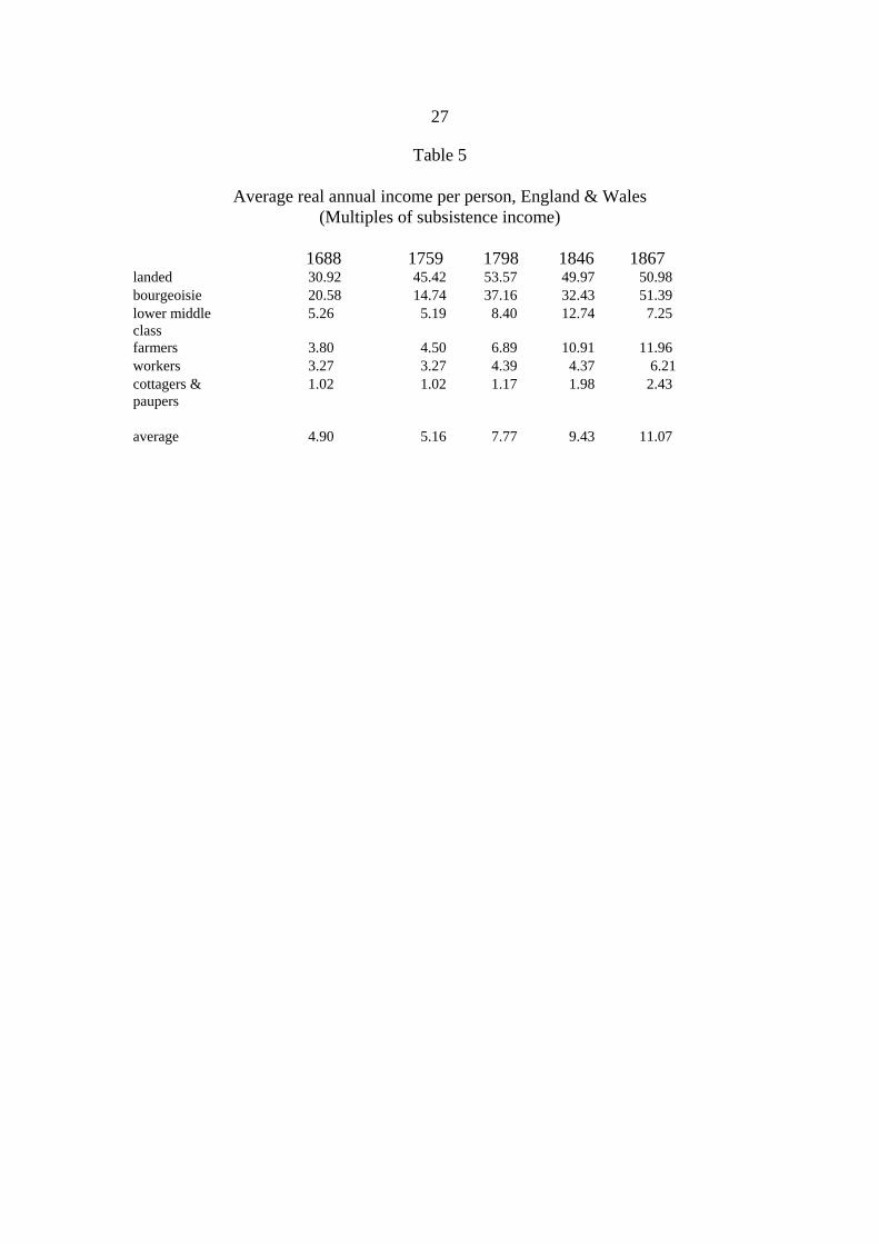
A first goal of this paper is to form estimates of the size of the workforce from theearly social tables. Servants are tallied as family members in the tables of King, Massie, andColquhoun. In King’s table, for instance, the temporal lords are shown as having an averageof 40 people per family. Most of these were domestic servants, and it is necessary to removethem and list them separately to measure the labour force. I did this by estimating theaverage number of kin per family and classifying any additional household members asservants.

In the tables of King and Massie, there were 4.5 people per household in thecategories of shop keepers and tradesmen, manufacturers (i.e. the people who were employedin handicraft manufacturing), the building trades, and miners. These groups amounted to28% of the population in King’s table. Some households were smaller, in particular, those oflabourers and out servants, cottagers and paupers, and those in the military and merchantmarine. All other groups had families with more than 4.5 people. Since the groups with anaverage family size of 4.5 probably did not keep servants, that is a plausible value for theaverage number of kin in a household.

This conjecture is corroborated by studies of the average size of a household in earlymodern England. Laslett analysed information on 100 communities and found that theaverage household contained 4.75 people.16 This figure included servants, so the number ofkin per household was smaller. Labourers had virtually no servants in their households, andthe average size of a labourer’s household was 4.51, thus substantiating our assumption. Paupers had fewer kin in a household, which is also in line with King, while husbandmen,yeomen, and higher status groups had bigger households. They also employed servants.17

Hollingsworth studied the demography of English ducal families including the size oftheir households by reconstituting them from family trees. Hollingsworth’s data show

13Broadberry et al, British economic growth, p. 326..

14 Feinstein, ‘Pessimism,’ pp. 652-3.

15In the section on ‘validating comparisons,’ I explain how I extracted the GDP ofEngland and Wales from Broadberry’s series for Great Britain,

16Laslett, ‘Size and structure,’p. 200.

17Ibid., pp. 221-2.

5

considerable fluctuation over time and are not reported in a way that permits exactcomparison with Laslett’s. However, mean family size for ‘completed’ families where thewife lived past 45 years of age are consistent with the assumption of 4.5 kin per family.18

Wills point in the same direction. Wrigley et al found that the average male testatorhad 2.58 surviving children, which suggests a family of 4.58 including both parents.19 Clarkcame to similar conclusions.20

In view of this evidence, I adopted the value of 4.5 kin per household in all socialgroups above the paupers, who had smaller families. If the average size of a family wasgreater than 4.5, the difference between the average size and 4.5 was, therefore, assumed toequal the number of servants. In the case of freeholders and farmers, these were taken to befarm servants; otherwise, they were assumed to be domestic servants. Families with less than4.5 members were also assumed to have no servants.

The application of these principles to King’s table yielded 191,889 domestic servantsand 168,856 farm servants. In the case of Massie, the corresponding figures were 209,575and 243,170, and with Colquhoun the result was 384,057 domestic servants and 340,000 farmservants.

Size of the workforce: women and children

In the tables of King, Massie, and Colquhoun, the population is divided into statusand occupational groups that reflected the husband’s status. In 1798, these totalled 2,227,630compared to a total population of 8,379,739 as tallied in the table. The ratio, 27%, is muchless than the ratio of the occupied to the total population (45%) that Deane and Cole surmisedfor Great Britain in that year (and which was very stable across the first half of the nineteenthcentury).21 Applying this percentage to Colquhoun’s population total implies an additional1,869,078 occupied people. 724,057 of them we have already discovered, namely, theservants. The rest were presumably women and children. The question is how many of themwere there really and in what sectors?

I assume that the wives and children of the landed classes and the upper strata of themiddle class–namely those with an income above that of a shopkeeper–did not work. Alsothe naval and army officers, soldiers, seamen, who are credited with very small families, ifany, are assumed not to have had working wives or children. That leaves the lower middleclass and working class. It is clear from the incomes of many of these groups that thefamilies must have had multiple earners. Thus in 1798, the very large group of employees inmanufacturing and building had an average income of £55 per year. However, exceptionalcircumstances aside, a fully employed man could have earned at most £30 - £35 in thosesectors.22 The rest of the income must have come from other family members. Baxter’s

18Hollingsworth, ‘Ducal families,’ p. 19.

19Wrigley et al, Family reconstitution, p. 614.

20Clark, Farewell, pp. 116-21, Son, p. 133.

21Deane and Cole, British economic growth, pp. 8, 143.

22See the sources cited in Feinstein, ‘Wage-earnings.’

6

analysis of manual occupations showed that only about 40% of workers in manufacturingwere men.23 The rest were women and children. Hence, total employment in manufacturingwas 2.5 times male employment with the additions being women and children. Assuming thesame ratio obtained in Colquohoun’s table implies that the average earnings of a worker inmanufacturing was £22 per year, which is slightly more than the average earnings of allworkers in cotton mills in that year.24 The result is not implausible. The wives (but not thechildren) of shopkeepers, clerks, publicans, peddlers, and tailors were also assumed to haveworked in their husbands’ businesses, and this reduces the earnings per worker to a plausibleamount, general £37.5 per year. The lower middle class was earning more than the averageworker but not a lot more. The wives of miners were also assumed to have worked.

Initially, the labour force participation of family members among the freeholders andfarmers was explored with the same considerations in mind. The execution was complicatedsince farms were businesses and the family members the residual claimants. The aim was toset the number of family members working in the business such that the net business incomeper working family member equalled the wage of a farm labourer. Farm income wasanalysed as follows: The income of farmers and freeholders in the social tables was assumedto exclude the (generally cash) payments to labourers but to include the income of servants,much of which was paid to them in kind. Allen’s reconstruction of England’s agricultualaccounts points to factor shares for agriculture of 39% for labour, 15% for capital, and 46%for land.25 These shares were applied to the total income of freeholders and husbandmen(assumed to be owner occupying cultivators) to split it into returns to labour, capital, andland. Farmers were assumed to be tenants, so their income was divided between labour andcapital in the ratio of 39:15. The earnings of servants were subtracted from the labourincome derived in this way, and the residual was divided by the assumed number of familymembers working on the farm to compute annual wage income per worker. In the tables ofKing and Massie, the calculations imply that two family members were working in the caseof tenant farmers. However, in the case of freeholders and husbandmen only one familymember was working. In Colquhoun’s table, the calculations point to two family membersworking amongst the tenant farmers and the greater freeholders and only one workingamongst the lesser freeholders.

It seemed very odd that wives were working on tenanted farms but not on freeholdfarms. If we assume that wives were working on all types of farms, then wage income perfamily member was very low on the freehold farms and among the husbandmen. However,the cash flow of these enterprises was in reality much higher since they are assumed to beowner-occupied, so the farm families were also receiving the rental value of the property asincome. If we calculate net business income including land rental value per working familymember, we find that the earnings of each family member approximately equalled the wage

23 Baxter, National income, pp. 88-95.

24Assuming a 50 week year, a weighted average of the earnings of men, women, andchildren in cotton spinning in 1797 was £21-1s.-9d. according to Feinstein, ‘Wage-earnings,’p. 190.

25In this calculation, the inputs are valued at exogenous supply prices, so the shares donot include supernormal profits such as those earned in 1801. Allen, ‘English and Welsh,’ p.41.

7

of an agricultural labourer. Based on these results, I decided to assign two family membersas the workforce on all types of farms. In the case of the husbandmen and freeholders, thismeans that the average product of labour equalled the agricultural wage, while the marginalproduct of labour was much less. From a resource allocation point of view, there was toomuch labour in the agricultural sector in England during the eighteenth century. This is atypical situation at the start of industrial development. The misallocation was disappearingby 1800 and had vanished by 1846.

Occupations, incomes, and households in Smee and Baxter

Smee and Baxter based their national income estimates on the occupational returns inthe 1841 and 1861 censuses. This procedure creates issues with respect to occupations,incomes, and household definition. These should be dealt with in a way that ensurescomparability with the earlier tables.

Since Smee and Baxter wanted to estimate the national income in 1846 and 1867,respectively, they increased the occupational counts for 1841 and 1861 by assumed rates ofpopulation growth. The subdivisions of the occupied population in the censuses included notonly bricklayers and weavers but also landed proprietors, capitalists, and those withindependent incomes–anyone with an income. How can the incomes of these occupations bedetermined? Both Smee and Baxter proceeded in a similar way. The distinguished the upperclasses from the working class. The income of the latter was estimated by assigning a wageto each working class occupation and then calculating total annual wage income. Baxter didthis with great care and worried over how many weeks were worked each year, who wasunemployed, the age at which people stopped working, and so forth. The 1861 censustabulated occupations by industries, so he could readily assign wages to occupations. Baxterpresents two complementary lists of occupations and earnings,26 and I have combined them toproduce his overview of employment and labour earnings in England and Wales brokendown by detailed industry and distinguishing men, women, boys, and girls.

Smee’s work was much more summary. The 1841 census has an alphabetical listingof occupations. In principle this could be retabulated on an industrial basis like the 1861census, but the task is forbidding, and no one has yet done so. Instead, Smee relied on therather gross breakdown of occupations in the Occupation Abstract of the 1841 census andassigned labour incomes accordingly.27 His weekly wages look to have been chosen tocorrespond to the annual labour earnings he used on the assumption that people worked 52weeks per year. This was surely not true. Comparison with other data, however, indicatesthat the annual earnings are plausible.28 When weekly wages are calculated on theassumption that people worked as Baxter assumed, the weekly earnings also fall into linewith other evidence. Smee’s tabulations were for Great Britain. I have followed Smee’sprocedures and recreated his table using only the occupational returns for England and Walesto bring the results into conformity with the other social tables. It turns out that more detail isavailable on the breakdown of children’s employment than Smee availed himself of, and this

26Baxter, National income, pp. 88-95.

27Occupation Abstract, (P.P. 1844, 587, image 58-62.).

28Feinstein, ‘Pessimism,’ ‘Wage-earnings.’

8

information is used in my reworking of Smee.In the cases of both Smee and Baxter, middle and upper class incomes were estimated

separately using the aggregate records of income tax paid. The tax was reported on variousschedules, which had a loose correspondence to type of economic activity. There was a taxthreshold, and another difficulty is that lower middle class income was below the threshold,so had to be estimated with cruder procedures. Baxter’s work is again the most thorough,and it has been carefully examined by Lindert and Williamson.29 I rely entirely on PeterLindert’s spreadsheet and conclusions for the middle and upper class income in 1867.30 Smee’s estimates of middle and upper class income for Great Britain have been scaled downin proportion to population to get values for England and Wales.

While Baxter’s work is more thorough than Smee’s in most respects, there is one wayin which Smee provides more detail, and that is in the assignment of middle class income toindustries. Smee makes that assignment, while Baxter does not, and that presents challengesfor consistent comparison, as we will see.

The census-based approach of Smee and Baxter throws up a final issue, namely, howthe data on men, women, and children, which are tabulated separately, should be combined toform households that are comparable to those in the eighteenth century tables. Lindert hastaken the most careful approach, and he identifies a considerable number of female headedhouseholds within the working class. The total income earned by all non-household headswas apportioned evenly across the household heads. In contrast, among the middle and upperclasses, Lindert assumed that all income earned by non-household heads accrued tohousehold heads in the same income class.

A limitation of Lindert’s approach, as applied to the working class, is that it does notcorrespond to the eighteenth century patriarchal assumption that all households were headedby men.31 (His treatment of the middle and upper classes is consistent with that assumption.) I, therefore, retabulated the 1867 data in the format of an eighteenth century table.32 It is veryfortunate that this change in procedure has virtually no impact on measured inequality: TheGini coefficients were virtually identical in the two cases. Reassured by this result, Itabulated Smee’s occupational and income data in the eighteenth century patriarchal manner.

Consistent occupational classification

The various social tables break the population down in ways that are not immediately

29Lindert and Williamson, ‘Reinterpreting,’ pp. 94-5.

30Lindert, ‘Baxter,’ Main:A2..AB50.

31I violated this assumption in the case of female servants who were entered in thesocial table as independent households (as were male servants). This convention is followedin all of the social tables.

32Leaving aside female servants who remain a separate category, the earnings ofwomen and children in the working class were divided by the number of men in the workingclass (omitting male servants who are also a separate category). The earnings of each man inthe working class (other than male servants) was then increased by this average to estimatehis household’s income.

9

comparable. Partly this reflects differences in the sources used and partly it reflects theevolution of the economy. While the 1861 census, for instance, distinguishes foodmanufacturers from food retailers, these activities were united in King’s ‘shopkeepers andtradesmen.’ The butcher’s shop, for instance, combined an abattoir, which is manufacturing,with retail sales. This renders meaningless attempts to neatly divide the early moderneconomy into ‘agriculture,’ ‘manufacturing,’ and ‘services.’

I have classified the occupations and incomes in all of the tables into six categories:landed classes, bourgeoisie, lower middle class, farmers, workers, and paupers. Numbers andincomes appear in Appendix Tables 1-6. ‘Earners’ refers to those who work or to whomproperty income or poor relief accrued. ‘People’ refers to household members excludingservants. Servants are treated as single member households.

Landed classesIn King, Massie, and Colquhoun, this group includes the titled aristocracy as well as

‘gentlemen,’ ie the gentry. The landed classes also include the clergy of the Church ofEngland, who were supported by glebe estates, and university teachers who were alsosupported with landed property.

In Smee and Baxter, the number of households in the landed classes was taken toequal the sum of men and women returned in the 1841 and 1861 censuses as landedproprietors plus the numbers of Church of England clergy and university teachers. Theincome of the landed classes was taken to be 80% of the rental value of the agricultural landin the country on the presumption that the other 20% accrued to owner occupying farmers.33

My estimate of the total income of the landed classes omits the value of urban real estate andnonagricultural investments.

BourgeoisieIn my summary of King, Massie, and Colquhoun, the bourgeoisie includes state office

holders, lawyers, dissenting clergy, merchants big and small, ship owners, warehouseowners, capitalists, shipbuilders, naval and military officers, and half pay officers. To judgeby their incomes, ‘manufacturers’ in King were handicraft workers, while in Colquhoun theywere capitalists. Massie produces a breakdown by income of manufacturers, so those whowere large scale employers could be separated from the handicraft workers.

Colquhuon listed 50,000 people as trustees of funds. The corresponding income hasbeen divided among the peers (£1 million), gentlemen (£1 million), big merchants(£1055000), little merchants (£1000000), and manufacturers (£1000000) on the assumptionthat the trustees were drawn from these groups.

In the case of Smee, the bourgeoisie includes the non-wage earning men and womenin all income categories in the occupations of trade, manufacturing, and commerce, the army,navy, merchant marine, professionals, other educated people, government civil servants,police and parochial officers, and men of independent incomes less the number in the landedclasses and in the lower middle class (defined below).

It should be noted that Smee reports an unusually large number of women andchildren in the middle class with independent incomes. These people may have been underenumerated in the earlier tables. Smee’s number considerably exceeds Baxter’s, who madesimilar estimates two decades later and who was in most respects more careful and

33Mingay, Landed society, p. 26, Thompson, ‘Social Distribution,’ Beckett, ‘Pattern.’

10

systematic. The result is to inflate considerably the number of middle class earners in 1846.In my analysis of Baxter, the bourgeoisie is measured indirectly. Baxter divided the

population and the corresponding income into the manual working class, on the one hand,and the middle and upper classes on the other. I specify the bourgeoisie to equal Baxter’smiddle and upper class minus my measures of the landed classes, the lower middle class, andthe farmers.

Lower middle classThe number of occupations in this group expanded over time. In King’s and Massie’s

tables, it consisted of shopkeepers and tradesmen plus those in science and the arts. Thelatter might have been assigned to the bourgeoisie but were put in the lower middle class inview of their income. With Colquhoun, the definition of lower middle class was expanded toinclude the newly distinguished occupations of school teachers, theater, lunatic asylums,clerks, publicans, peddlers, tailors, and engineers.

Both Smee and Baxter divided the population into the working class, on the one hand,and the middle and upper classes, on the other. The problem is extracting the lower middleclass from the latter. I set the lower middle class equal to 80% of the lowest income categoryamong the upper and middle classes that they delineated.34 The implication of this is that thelower middle class amounted to about two-thirds of the middle and upper classes and wasmuch the poorest grouping of that assemblage. As it happens, the lower middle class came toa similar fraction of the middle and upper classes in Colquhoun’s table even though it wasconstructed on a very different basis.

Farmers

The category of farmers includes greater and lesser freeholders and farmers in thetables of King, Massie, and Colquhoun. Massie also distinguished the category ofhusbandmen. These were small scale cultivators. Massie shows their number at 200thousand, which Lindert and Williamson reduced to 134,160, a figure which I adopt.35 Kingdoes not report husbandmen, although they were present in the country. I expect they weretallied as cottagers in his table. I have assumed there were 175,000 husbandmen in 1688 andremoved that number from the cottager category. I assumed the average family income ofhusbandmen was £12 and the average family consisted of four members. Colquhoun also listsno husbandmen, but the total of the freeholders and farmers in his table (320,000) is greaterthan the 250,000 farmers who cultivated England in the 1830s and so apparently includesperhaps 70,000 husbandmen. There was a substantial decline in the number of small owner-occupying farmers in the eighteenth century.

34More precisely, in the case of Smee, the lower middle class households wereassumed to equal 80% of the non-wage earning men, 20 years and older, in the £50-£150 peryear range, in the categories of trade, manufacturing, and commerce, the army, navy,merchant marine, professionals, other educated people, government civil servants, police andparochial officers, and men of independent incomes. With Baxter, the number of householdsin the lower middle class was taken to equal 80% of the ‘small incomes (2)’ category with anaverage income of £75.

35Lindert and Williamson, ‘Revising’ , p. 397.

11

The share of rent received by the owner-occupying farmers declined less steeply. Itfell from 35% in 1688 to 31% in 1759 to 28% in 1798, after which the share was presumed tohave remained at 20%. These proportions are in close agreement with Thompson’s summaryof the land belonging to owner-occupying small holders.36

With Smee, the farmer households included all of the nonwage-earning men in theoccupations ‘farmers & graziers’ and ‘florists & gardeners.’ In the case of Baxter, I assumedthat the number of farmers was the number of ‘farmers & graziers’ and ‘florists & gardeners’returned for England and Wales in the 1861 census, and the corresponding income wasfarmers’ profits as recorded on Schedule B of the income tax.37

Workers

With King, Massie, and Colquhoun, I defined ‘workers’ as the manufacturingworkforce, the building trades, miners, labourers and out servants, soldiers, seamen, domesticservants, and farm servants. In King, the ‘manufacturing workforce,’in turn, was taken to be‘manufacturers;’ in Massie, it meant manufacturers less those with high incomes who wereassumed to be capitalists, and, in Colquhoun, it meant ‘workers in manufacturing.’

Smee calculated the number of working class men and women separately for eachindustry, as the number of adult men and women assigned to that industry less his estimate ofmiddle class men or women in that industry. He assumed that the boys and girls reported foreach industry were in the working class and made a separate, global estimate of middle andupper class minors receiving property income. He estimated working class income bychoosing a representative wage for men, women, boys, and girls in each industry. Hisweekly wages are plausible if they are assumed to equal annual wages divided by 52.

The 1861 census tabulated the occupations by industry and was, therefore, mucheasier to work with than the 1841 census with its alphabetical listing of occupations. Baxtertabulated the occupational data by industry and assigned industry specific wage rates tooccupations. He carefully considered the question of how many weeks people actuallyworked and annual wage income was calculated accordingly.38 Working class incomeequalled these totals less the number of paupers and their income.

The poor

In the cases of King and Massie, I specify the ‘poor’ to include the categories of‘cottagers and paupers’ plus ‘vagrants.’ In the case of King, this number was reduced by the175,000 assumed to be husbandmen.

With Colquhoun, the ‘poor’ included ‘paupers at work,’ ‘vagrants,’ ‘debtors’ and‘lunatics.’ The number is approximately the number of people relieved under the poor law,and the total income that Colquhoun assigns them approximated the annual expenditure on

36Thompson, ‘Social Distribution, p. 513.

37Baxter, National income, p. 25.

38See the totals for manual workers in Peter Lindert’s spreadsheet Baxter E&W UK1867, in cell ‘main:V11' and ‘main:X30.’

12

the poor.39

Smee’s estimate of the number of paupers was the number returned in the 1841census category of ‘alms, pensioners, paupers, lunatics, prisoners.’ This is manifestly toosmall. I have instead set the number of poor equal to the number of people relieved under thepoor law, and their income equal to the cost of poor relief. Working class numbers andincome were adjusted accordingly. The same procedure was followed with Baxter. In bothcases, the cost of poor relief and the number relieved were estimated by applying the nationalrates per thousand given in Porter’s Progress of the nation for the closest year to theappropriate populations of England and Wales.40

Breaking Income Down into Rents, Wages, and Profits

It is important to break down the incomes of the social groups into returns to land,labour, and capital. This is essential to validate the tables, to reconstruct the size of theagricultural sector, and it throws light on the political economy of the period. The tables ofKing, Massie and Colquhoun present different problems from those of Smee and Baxter. Inmy reconstruction of the tables of King and Massie, the landed classes were assumed toderive all of their incomes from land rents. In Colquhoun’s table, it was assumed that 90% ofthe landed income was rent and 10% was profits. The earnings of workers, artisans, andlabourers were all tallied as wages. The incomes of employers in the bourgeoisie wereassumed to be a mixture of profits and salaries. They were distinguished by assumingsalaries for each occupation and computing profits as the residual. King usuallydistinguished ‘greater’ from ‘lesser’ merchants, etc., and I assumed that the annual salary of agreater merchant was £60 and a lesser £30. These were increased by 13% in Smee’s table,and were raised to £70 and £35 in Colquhoun’s table.41 Groups that were not designatedgreater or lesser were assigned the salary that seemed appropriate given the activity and totalincome. The incomes of farmers, freeholders, and husbandmen were divided into factorearnings using agricultural factor shares as explained earlier.

Smee and Baxter distinguished working class wages from middle and upper classincomes. The difficulties arise in breaking the middle and upper class incomes down intorent, profits, and salaries. Returns to agricultural land were estimated extraneously from datain the Agrarian History of England and Wales.42 In the case of Smee, the remaining incomewas divided on the assumption that salaries were £50 per year for men, most of whomcorrespond to those earning £35 per year in 1798, and two-thirds of that for women. Thesalary was increased to £75 in the case of Baxter and £100 for the small number in the

39Perkin, Origins, p. 421,ftn 3, Porter, Progress, p. 64.

40Porter, Progress, pp. 63, 67.

41On the one hand, these salaries are arbitrary, and they are low relative to the incomeof these groups. On the other hand, salaries of this magnitude are unavoidable. Theremaining income of the bourgeoisie was profits, and they amounted to approximately threequarters of the profits in the economy. Higher salaries would have implied lower profits, andlower profits, in turn, would have implied an implausibly low rate of return to capital.

42Afton and Turner, ‘Rent’ p. 1920.

13

highest earning group.43

validating comparisons

Revising the social tables involves a good deal of conjecture as extraneousinformation of varying degrees of reliability are incorporated in the amendments. Howreliable are the resulting social tables? One way to answer that question is to work out theimplications of the social tables for issues that can be approached with other sources ofinformation. If the implications of the social tables agree with the other sources, then there issome reason to have confidence in the revised social tables. I examine five indicators.

The first indicator is nominal GDP. Broadberry et al. have estimated annual GDP forEngland and Wales in 1688 and Great Britain for the years of the later social tables.44 Theirestimates are based on wholly different sources–physical output indices multiplied by priceindices. How do the revised social tables compare to their series?45 Figure 1 shows thatagreement is quite close. Broadberry et al made similar comparisons for King, Massie, andColquhoun. Massie’s incomes were raised to bring them into conformity with the annualestimates–an adjustment that is warranted by the wage history of the period–and Colquhoun’swas raised even more dramatically to the same end. I have followed their lead in dealingwith Massie but not with Colquhoun, as Broadberry et al’s adjustment is not in accord withthe wage data. Their procedure amounts to raising Colquhoun’s estimate to hit the transitorypeak in 1801 show in Figure 1. Assuming that Colquhoun’s estimate applies to 1798 ratherthan 1801 brings the social table into conformity with the annual series.

<Figure 1 about here>

43A division along these lines is required for a plausible rate of return to capital.

44For the comparisons discussed here, nominal GDP for England and Wales wasworked out as follows. Broadberry et al, British economic growth, p p. 201, 227-44,reported nominal GDP for England and Wales in 1688 and 1700 and nominal GDP for GreatBritain in 1700. Nominal GDP for Great Britain in subsequent years was then computed byincreasing the 1700 nominal value by the proportional change in the index of real GDPmultiplied by the proportional change in the index of the price level. This nominal GDPseries for Great Britain was then used to extrapolate the nominal GDP estimate for Englandand Wales in 1700 to later years.

45The incomes in the social tables include transfer payments from the state–namelyinterest on the national debt and poor law support–without corresponding deductions fortaxes. Since most taxes were indirect, no straightforward deductions are possible. Transferpayments must be excluded in comparing the total income in the social tables with GDP. Poor law payments in England & Wales and their share of the United Kingdom debt chargeshave been deducted in Figure 1. See Deane and Coale, British economic growth, pp.389-91,396-7) for debt service charges. England & Wales assumed to be 85% of Great Britain in theeighteenth century, 77% and 82.3% of the United Kingdom in 1846 and 1867, respectively,in accord with the country’s share of UK GDP. These adjustments have only a minor impacton the comparisons in Figure 1.

14

The second indicator is the labour force participation rate. This is an important checkin view of the large number of servants and women and children who have been added to thelabour force by my procedures. Deane and Cole estimated the occupied population of GreatBritain at ten year intervals beginning in 1801.46 The ratio of the occupied to the totalpopulation was fairly stable ranging between 44% and 47% over the nineteenth century.

The revised social tables imply similar percentages: 48% in the case of King, 49% inMassie, 49% in Colquhoun, 41% in Smee, and 46% in Baxter. Smee’s ratio is on the lowside while Massie’s and Colquhoun’s are a bit high, but on average the labour forceparticipation rate implied by the social tables are consistent with Deane and Cole’sestimates.47

The third indicator is annual wage income averaged across all manual workers(earners in the social tables). Feinstein’s series is widely cited, and it agrees with Lindert andWilliamson’s, which is the other broadly based index48. For the purposes of comparison,Feinstein’s nominal wage series has two limitations. First, it only begins in 1770. I haveextended it back to 1688 with a weighted average of the wages of building craftsmen andlabourers in London, southern English towns, and northern England, as well as farmlabourers, as previously described. Second, Feinstein’s series overstates average earnings. While it is about right for cotton textiles where he averaged the full spectrum of male,female, and child wages, in most other industries Feinstein’s series was calculated mainlyfrom the earnings of adult men. I have rebased Feinstein’s nominal wage series to equalaverage earnings for all workers in 1851 as calculated by Deane and Cole.49 The extrapolatedvalue for 1867 turns out to be within 4% of Baxter’s calculation for all manual workers forthat year–£34.07 versus £32.72 in Baxter. Figure 2 compares the extended Feinstein nominalwage series to the average wages per earner implied by the social tables. The agreement isclose.

<Figure 2 about here>

The fourth indicator is the rate of return on capital. The social tables imply totalprofits in the economy. Dividing total (nominal) profits by the nominal capital stock yields arate of return to capital. Giffen estimated the stock of reproducible capital in 1688, andFeinstein estimated capital stocks for Great Britain and the UK that can be used to work outthe capital stock in England and Wales at the dates of the social tables.50 The rate of profit

46Deane and Cole, British economic growth, pp. 8, 143.

47It should be noted Broadberry et al, British economic growth, pp. 352-60, presentedestimates derived from King, Massie, and Colquhoun that imply ratios of the occupiedpopulation to the total of 34%, 33%, and 31% respectively. Deane and Cole’s, Britisheconomic growth, pp. 8, 143, estimate for 1801 implies a rate of 45%. I prefer Deane andCole.

48Feinstein, ‘Pessimosm,’ Lindert and Williamson, ‘Living standaard.’

49Deane and Cole, British economic growth, pp. 143, 152.

50Feinstein, ‘Capital formation, p. 33, Feinstein, ‘Sources,’ p. 427.

15

rose from a pre-industrial level of 9.2% in 1688 and 9.1% in 1759 and to 16.8% in 1798. Therate continued to rise gradually reaching 17.6% in 1846 and 20.3% in 1867.51 The rates ofreturn are higher than interest rates on government debt and mortgages but in line withestimates of the return on business investments and with aggregate calculations of the realrate of return by Allen.52

The fifth indicator is agricultural income. Since agricultural occupations and incomesources can be identified in the social tables, total agricultural income can be calculated. With King, Massie, and Colquhoun, I compute agricultural income as the agricultural rentalincome of the landed classes plus the incomes of the farmers, freeholders, husbandmen, farmservants, and agricultural labourers. All of these are separately identified except foragricultural labourers in the tables of King and Massie, which report the number and incomeof labourers in all sectors of the economy. The indefiniteness of King and Massie in thisregard may reflect a reality in which, over the course of the year, labourers worked more thanone job–farming, carting, weaving, for instance–in more than one sector, so their labourcannot be easily allocated. However, following Broadberry, Campbell, and van Leeuwenapproximately, I assumed that 64% of the labourers and their income were agricultural.53 This division means that 64% of the work and income of labourers in total came fromagriculture, however each worker split his time. Sectoral allocation, however, is problematic.

In cases of Smee and Baxter, agricultural income was calculated as the sum of theincomes of the landed classes, farmers, and farm labourers. Total agricultural income isshown in Table 1.

< Table 1 about here.>

Table 1 also shows direct estimates of agricultural income for comparison. Theestimates corresponding to the social tables of King, Massie, Colquhoun, and Smee are takenfrom Allen’s agricultural reconstruction.54 This study estimated the net output of theprincipal agricultural commodities in England and Wales at benchmark dates from the middleages through the Industrial Revolution. Output was valued with prices prevailing at the time. The quantities of farm inputs were also estimated and their values calculated. Manyuncertainties surround this exercise, but they can be reduced by ensuring that totalagricultural income equalled the value of net production. This is an important check onreliability. Social tables were not used in this exercise. The independent estimate for 1867 isFeinstein’s (1972, T60) estimate for the UK multiplied by the share of England & Wales in

51Interest on the national debt is included in household income in the social tables. Itis not a return to land or labour and so ends up in ‘profits’ when the income in the socialtables is split into factor returns. Interest on the national debt is deducted from ‘profits’ socalculated in the rate of return calculations presented here..

52Harley, ‘Cotton textiles,’ Hudson, Genesis, pp. 235-41, 272, 277, Allen, ‘Engels’Pause,’ p. 421.

53 Broadberry et al, British economic growth, pp. 20-1.

54 Allen, ‘English and Welsh,’p. 36.

16

UK agriculture.55

In the event, most of the direct estimates match up with the incomes in the socialtables. Allen’s estimate for 1800 is higher than Colquhoun’s, probably because Colquhoun’sapplies to 1798 when farm prices were lower. The discrepancy between the 1850 estimateand Smee’s does not have an obvious explanation.

The incomes and employment levels in the social tables imply trajectories for thedeclining importance of agriculture during the industrial revolution. This can be measuredeither as the ratio of agricultural value added to GDP or as the ratio of the agricultural labourforce to the total occupied population. Table 2 summarizes the evidence in the social tables. By both measures agriculture declined during the Industrial Revolution. However, there is anunexpected twist in the tale, namely, the decline was greater by the value added measure thanby the labour force measure. In 1688, the agricultural share of GDP was 46%, while thelabour force share was 39%. In 1867, agriculture accounted for only 15% of GDP but 20%of the work force.

<Table 2 about here.>

The surprising feature of this result is that the value added share in 1688 was greaterthan the labour force share. Kuznets’ investigations of less developed countries in thetwentieth century indicated the reverse.56 He found that the agricultural labour force sharewas higher than the value added share, and this indicated that GDP would rise if labour wasreallocated from agriculture to manufacturing. How could England have been different in1688? From a numerical point of view, the answer is clear. Wages were somewhat lower inagriculture than in other sectors–this is in accord with the Kuznets view–however, this effectwas outweighed by the vast amount of rent generated in agriculture. It is the rent taken bythe gentry and aristocracy that increases the share of agriculture in the economy whenmeasured by value added. (Leaving out the rent reduces the value added share of agricultureto 23%.) England in 1688 was unusual compared to many peasant societies in terms of thecomprehensiveness and efficiency with which its aristocracy extracted income from thefarming population.

Implications: size and incomes of the social classes

The object of harmonising the social tables is to permit comparisons of key variablesacross the Industrial Revolution. Some comparisons are shown in accompanying tables, andmore can be worked out from the information reported in this paper.

Table 3 shows the numbers of people reported in the six major social groups. Theirrelative sizes changed greatly over the Industrial Revolution.

<Table 3 about here>

The ‘landed classes’ were never more than 2% of the population, and the proportion

55 Feinstein, Statistical Tables, T60.

56Kuznets, Economic Growth, pp. 111, 203, 208-16.

17

stayed roughly constant over time. The increase from 30,000 to 50,000 shown in Table 3probably reflects the inclusion of female property owners in 1846 and 1867 who were left outof the earlier counts.

The ‘bourgeoisie,’ which included the large scale capitalists, bankers, merchants,lawyers, high officials, and investors, already outnumbered the landed classes in 1688, andthis stratum grew seven-fold during the Industrial Revolution. Their share of the populationincreased from 3% to about 8-9% over the Industrial Revolution.

The third group was the lower middle class. This category increased almost eight-fold from 1688 to 1867.

The fourth group, farmers, formed a declining share of the population. In 1688 therewere close to 200 thousand small holdings held by husbandmen and yeoman and cultivatedby them and their families. The other 200 thousand were larger farms mainly leased fromgreat estates and cultivated by hired labour. The number of farms declined in the eighteenthand early nineteenth centuries as yeoman holdings were amalgamated into large farms. Agriculture was a declining sector during the Industrial Revolution.

The fifth group was the workers. It was the largest group in the English economy,and it increased by a factor of almost four during the Industrial Revolution. Most of the newjobs were nonagricultural. The character of work changed significantly as the independentcraftsman working with hand equipment in his or her cottage gave way to machine operatorsemployed in the new factories.

The poorest group were only partially employed, if they worked at all. In 1688 thisgroup comprised almost one tenth of the families. The share of the population who werepaupers was constant to 1759 and then increased as the population expanded, theemployment opportunities for women as spinners declined, and food prices rose asagricultural output lagged behind population. The decline in the number of poor shown inthe table between 1798 and 1846 was the consequence of reforms to the Poor Law, whichmade it harder to get relief. The decline is thus spurious. However, the further decline to1867 in the fraction who were poor probably reflects a rising demand for labour.

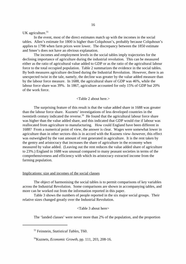
We can also use the social tables to track the incomes of these groups. This can bedone either in terms of earnings or purchasing power. Table 4 shows the average income ofan earner in each group. Households could, and did, have multiple earners, for instance,when the husband wove, his wife spun, and their son toiled in a mill. The standard of livingimplied by these earnings depended on the prices of the goods that people consumed. Thereare many ways to measure those prices, and here we measure it as the cost of the basket ofsubsistence goods that provides 2100 calories from the least expensive foods (primarilyoatmeal) and other bare necessities, and it is intended to represent the least cost way ofsurviving.57 Dividing earnings per person in the household by the cost of the basket adjustsearnings for price changes and shows how many baskets each person could consume in a year(Table 5).

<Tables 4 and 5 about here>

57The basket includes oats (170 kg), beans (20 kg), meat (5 kg), butter (3 kg), soap(1.3 kg), cotton cloth (3 metres), candles (1.3 kg), lamp oil (1.3 kg), fuel (2 million BTUs). In addition, the cost of these items was increased by 5% as an allowance for rent. See Allen,‘American exceptionalism.’

18

Table 5 shows how real incomes changed over the Industrial Revolution. The landedclasses were always well off. They could consume 30 baskets each in 1688, and theirconsumption possibilities increased to 50 in 1800 after which it remained stable. In reality,no one consumed 50 times the quantity of oatmeal in the subsistence basket. They upgradedtheir food consumption to more expensive sources of calories like quail and port and hiredbuilders, servants, and jewellery makers, who effectively ate the baskets (or upgradedversions) for them. By the 1860s, Table 5 probably understates the income of this groupsince it assumes they were only receiving agricultural rent and thus excludes their earningson urban property and nonagricultural investments, which were becoming important.

The landed classes consumed at a high level across the Industrial Revolution, but theirrelative position slowly eroded as agriculture declined vis-a-vis industry. In 1688 theagricultural rent received by the landed classes amounted to 16% of the national income. By1867, their rental income had dropped to 5%.

The bourgeoisie were the second richest group. They were not far behind the landedclasses. Their real incomes grew fairly steadily across the Industrial Revolution. Thebourgeoisie ended up slightly ahead of the landed classes with 51.39 baskets in 1867 versus50.98.

The incomes of the lower middle class and the farmers were between those of theupper classes and the workers. In the eighteenth century, the average earner in the lowermiddle class earned at least twice as much as the average worker. In 1688, the averagemember of the category of ‘farmers’ earned only a quarter more than the average worker. The‘farmer’ group average was depressed by the low earnings of the husbandmen and yeoman. As the small holders disappeared, the group average rose to twice that of workers in 1798. Inthe first half of the nineteenth century, as the nominal incomes of the landed classes and thecapitalists sagged, the lower middle class and the farmers surged ahead. After 1846, thefarmers continued to advance in the age of ‘high farming,’ while the shop keepers and clerksexperienced a fall in incomes. Their consumption standard was generally comfortable. Farmers tripled their incomes from 4 to almost 12 baskets over the Industrial Revolution. The shopkeepers and clerks started with five baskets in 1688, reached 12 in 1846 and thendropped back to 7 in 1867. This was scarcely above the earnings of a skilled craftsman.

The standard of living of the working class has been a particularly contentious issuein the historiography of the industrial revolution. The classic debate centred on the first halfof the nineteenth century and concerned the impact of industrialization. More recently,attention has turned to the eighteenth century: Was Britain a high wage economy in the run-up to the industrial revolution?58 The social tables of King, Massie, and Colquhounsummarize what these social observers believed wage levels to have been. In their eyes,England was definitely a high wage economy. English workers were always very well off byinternational standards: The average member of a working class family in England alwaysgot more than three subsistence baskets each year (Table 5), while many Europeans, LatinAmericans, and Asians were lucky to get one.59 Like the upper classes, English workers didnot consume three times the oatmeal specified in the subsistence diet but instead upgraded

58Humphries,’Lure, Allen, ‘Restatement,’ Humphries and Schneider, ‘Spinning,’Stephenson’ ‘”Real” wages?’.

59Allen, Bassino, Ma, Moll-Murata, and van Zanden, ‘China,’ Allen, Murphy, andSchneider, ‘Colonial Origins,’ Allen, ‘American exceptionalims.’

19

their consumption to bacon, beer, and white bread. For this reason, English men were alsotaller than their counterparts elsewhere in Europe, Asia, and Latin America.60

While English workers enjoyed a high standard of living at the start of the IndustrialRevolution, it was a long time before they realized substantial gains. There was no change inconsumption per person between 1688 and 1759, but it then rose from 3.27 to 4.39 baskets in1798. This was a period in which there was considerable wage convergence in Britain aswages in the North, which had been lower than those in London and the South generally,advanced to their level.61 Stagnation returned in the first half of the nineteenth century asworking class consumption per head edged downward by half a percent, while consumptionover all rose 21%, with the farmers and lower middle class reaping gains of over 50%. In1688 the average worker’s consumption was 67% of the national average. The ratio droppedto 63% in 1759, then to 56% in 1798 and bottomed out at 46% in 1846. The working classbegan to catch up between 1846 and 1867 by posting a consumption gain of 42% asconsumption per head jumped from 4.37 to 6.21 baskets. Growth in working classpurchasing power was well above the national average of 17% in this period. Working classconsumption per person rebounded to 56% of the national average in 1867.

The poor were at the bottom of the income distribution. Their income rose graduallyduring the Industrial Revolution. Between 1688 and 1798, there was very little growth ineither their nominal income or their standard of living. In the eighteenth century, the averagepoor person got just one subsistence basket per year. The poor did better, however, in thenineteenth century, and by 1867 each poor person got the equivalent of almost two and a halfsubsistence baskets. It is striking that the real consumption of the average poor personincreased by a factor of 2.38 between 1688 and 1867, which almost exactly equals the factor(2.26) by which average consumption increased for the English population as a whole overthe same period.

Implication: overall inequality

The changing fortunes of the different social classes can be summarized witheconomy-wide statistics. One candidate is the functional distribution of income indicated bythe shares of GDP going to labour, capital, and land (Table 6). The table gives equivocalsupport to the values commonly used in growth accounting (labour at 50%, capital at 35%,and land at 15%),62 but calls into question the corresponding assumption of a Cobb-Douglasproduction function, for the shares were certainly not constant. Labour’s share had a slightdownward trend, while the most dramatic changes were in the shares of capital and land. Capital’s share rose from 18.8% in 1688 to 38.6% in 1867, while land’s fell from 24.0% to6.3% over the same period. These trends in nominal shares are the same direction as thetrend in real shares computed by Allen, although the magnitudes of the changes in the real

60Floud, Fogel, Harris, and Hong, Changing Body, p. 69, Allen, ‘Restatement.’

61Gilboy, Wages.

62Beginning with Crafts, British economic growth..

20

shares of labour and capital were somewhat greater than the changes in the nominal shares.63 The share of capital increased a little at the expense of labour but mainly at the expense ofland. The shift from land to capital represents at redistribution of income at the top of theincome distribution, which renders the factor share approach a blunt instrument formeasuring changes in inequality. In addition, labour’s share includes salary income going tothe middle and upper classes, and so it is a misleading indicator of the fortunes of theworking class. Working class consumption per head compared to the national average is abetter indicator, as just discussed.

<Table 6 about here>

The Gini coefficient is another statistic that measures society-wide inequality and it isalso better suited to the task than factor shares. Ideally, the Gini is computed from theearnings of a representative sample of individuals. Such data do not exist for Britain duringthe Industrial Revolution. Gini’s can be computed from the earnings of the various socialgroups in a social table, although such calculations omit the effect of the variation of incomeswithin a group since the earnings of each individual are replaced by the group average. Milanovich, Lindert, and Williamson (2011), who used social tables to measure inequality inpre- and early industrializing societies, present a decomposition of the society-wide Gini intoterms measuring between group inequality, within group inequality, and inequality due to theoverlap of groups.64 They argue that between group inequality dominates the overall measurefor two reasons. First, they calculate bounds on within group inequality (using many of thetables we use here) that shows it to have been small. Second, they contend that the aim of thecompilers of the tables was to measure the important social cleavages, and that objective wasserved by highlighting between group inequality. Their conclusion is that tables like thoseused here, in which society is divided into a substantial number of groups, should revealbroad trends in inequality. Although it should be remembered that actual inequality mighthave been greater than measured inequality, I follow Milanovich, Lindert, and Williamson inusing the social tables to gauge overall inequality across the Industrial Revolution. A furtherreason for having confidence in the results is that the trends in the Gini’s make sense in termsof the group patterns we have already discussed

Conceptually, the first step in measuring inequality is to rank the individualhouseholds from richest to poorest. From this ordering, the Lorenz curve is drawn. Startingfrom the poorest, it shows the cumulative share of the total income received by thecumulative proportion of the population. Figure 3 shows Lorenz curves for England in 1688,1759, and 1798. The curves for 1688 and 1759 lie virtually on top of each other indicatingthere was no change in inequality between those dates. The curve for 1798 lies below these. That means that income was less equally distributed. In 1688 and 1759, the poorest 80% ofthe population received half of the total income. In 1798, the poorest 80% got only 35% of

63 Allen, ‘Engels’ pause.’ The nominal shares are more indicative of elasticities ofoutput with respect to inputs since the nominal prices (not the real prices) are those whichfirms are assumed to take as exogenous when costs are minimized in the usual productiontheory interpretation of the data. The nominal shares are, therefore, the appropriate shares forgrowth accounting.

64Milanovich, Lindert, and Williamson, “Pre-Industrial inequality.’

21

the total.

<Figure 3 about here>

It is useful to look at this from another angle. In 1688 and 1759, half of the totalincome accrued to the richest 20% of households, as noted. In 1798, half of the incomeaccrued to the richest 9% of households. Income was concentrated at the top of thedistribution in the last forty years of the eighteenth century. The immediate cause of this isclear from Table 4, namely, the dramatic rise in the income of the bourgeoisie from £145 perearner per year in 1759 to £525 in 1798. Possibly this concentration of income in thecapitalist class made a useful contribution to financing the Industrial Revolution, but this isan implication that we cannot explore here.

Inequality moderated in the middle of the nineteenth century. Figure 4 shows theLorenz curves for 1798, 1846, and 1867. Not much changed in the first half of the century,for the curves of Colquhoun and Smee lie for the most part on top of each other. The onlydifference is that the 1846 Lorenz curve shows slightly less concentrate of income at the verytop of the distribution. Evidently, in this period the surging incomes of farmers and the lowermiddle class did not change the rank ordering greatly. Inequality was much lower in 1867,however. In this case, the increase in wages meant that the bottom deciles of the incomedistribution took in a larger fraction of the total than they had previously received , and thisincrease is reflected in the steeper slope of the Lorenz curve for the poorer strata of society. The steeper slope lifted the Lorenz curve for 1867 above those for 1798 and 1846.

<Figure 4 about here>

The shifts in the Lorenz curves are summarized by Gini coefficients. A low lyingcurve like Colquhoun’s in 1798 has a large Gini indicating greater income inequality. TheGini coefficient was .54 in 1688, and .53 in 1759. By 1798, the Gini had jumped to .60 and itremained elevated at .58 in 1846. By 1867, it had dropped to .48.65 By this measure,England really did trace out a Kuznets curve with inequality rising in the late eighteenthcentury, remaining at a high value for the next half century, and then falling to 1867.

In recent years, inequality has risen in Britain as elsewhere, and that increase hascalled into question Kuznets’ optimistic–and evidently simplistic–theory. Inequalityremained at the 1867 level until the First World War, dropped dramatically as the Ginidipped below .3 in the interwar and early post-war periods, and has been rising since thenwith the Gini now equal to about .4. The history of the Gini in Britain is not unusual whencompared to other countries.66

Conclusion

Social tables are a long standing tool for analysing changes in social structure and

65While Lindert did not calculation a Gini from Smee’s table, he calculated them forthe other social tables discussed here, and my Gini’s are very close to his final calculations. Lindert, ‘Three centuries,’, p. 175.

66Milvanovic Global Inequality, p. 70-91.

22

income inequality. The more fully the tables are elaborated, the more powerfully theyilluminate social change. In this paper, we have extended the English social tables coveringthe industrial revolution by separating servants from the households in which they served andby quantifying the employment and earnings of women and children. These emendationsallow many more economy wide variables to be calculated. We have also groupedoccupations and statuses into a consistent set of categories to trace the fortunes of differentsocial groups across the industrial revolution.

The social tables throw light on many of the important questions concerning theindustrial revolution.

First, the tables confirm that England was a very prosperous country in the eighteenthcentury. Prosperity extended far down the social scale, in particular, the average member ofthe working class consumed over three baskets of subsistence goods per year, in a periodwhen workers in much of the rest of the world consumed little more than one. Only thepaupers and vagrants in England, who made up the poorest decile of the population, hadincomes that low.

Second, across the industrial revolution, the landed classes remained roughly constantin size, while the number of farmers declined modestly. On the other hand, the bourgeoisiegrew by a factor of seven, the lower middle class by eight, and the working class quadrupledbetween 1688 and 1867. The poor were on a roller coaster as their number tripled in theeighteenth century and then fell during the nineteenth.

Third, in the eighteenth century the greatest income gains were made by the landedclasses and the bourgeoisie, the two richest groups in society. The incomes of the landedclasses stabilized at a high level, while the average income of the bourgeoisie continued torise throughout the industrial revolution and caught up with the landed classes by 1867.

Fourth, during the first half of the nineteenth century, the greatest income gains wererealized by the lower middle class and farmers. The average real income of workers, on theother hand, stagnated. The ratio of the average consumption per head among workers slidfrom 67% of the overall average in 1688 to 56% in 1798 and then bottomed out at 46% in1846.

Fifth, the relative standing of workers improved dramatically between 1846 and 1867as working class consumption per head grew by 42%. In this period, they had the mostrapidly rising income of any group. Their relative consumption rose from 46% to 56% of theoverall average.

Sixth, the changes in the size and incomes of the main social groups translated intorising and then falling inequality. In 1688 and 1759, the Gini coefficient was about .54. Itjumped to .6 in 1798 as income was concentrated among the landed classes and thebourgeoisie. Inequality remained at this elevated level in the first half of the nineteenthcentury and then dropped between 1846 and 1867 when the Gini declined to .48. At last, thebenefits of economic growth were trickling down to the working class.

23

Table 1

Agricultural Output, England & Wales(Millions of £s)

A. Income from Social Tables

King Massie Colquhoun Smee Baxterrent 13.1 19.0 34.0 Landlords 36.9 34.4profits 2.7 3.6 6.3 Farmers 33.9 35.6 wages 9.8 12.4 29.6 Labourers 19.9 37.3

Total 25.6 35.0 69.8 90.6 107.3

B. Direct Estimates

1700 1750 1800 1850 1867value output 27.4 34.5 77.3 103.1 107.0

price index

real output

Sources of direct estimates:

1700-1850: Allen, ‘English and Welsh,’ p. 36.1867: Turner, After, p. 127, puts UK final agricultural output at £179 million in 1867-71 andIrish at £38.6 million, so British share was 78.4% of UK output. The Scottish agriculturalemployment share in Great Britain was the same as its population share–15%. This suggeststhe agricultural output of England and Wales was 67% (=.784*.85) of the UK total. According to Feinstein, Statistical Tables, T60, UK farm income in 1867 was £160 million,so farm income in England and Wales was £107 million.

24

Table 2

The share of agriculture in the English economy

1688 1759 1798 1846 1867value added 46% 46% 35% 21% 15%

labour force 39% 38% 33% 20% 20%

25

Table 3

Social Structure from Social Tables, England & Wales

A. number offamilies

1688 1759 1798 1846 1867 landed 31626 29070 38704 52986 50695 bourgeoisie 60128 84000 95879 363932 436493 lower middle 114602 188000 252640 649396 884450 farmer 402440 379008 320000 243130 223271 workers 980863 1128247 1804567 2598299 3668936 cottagers &paupers

161672 192310 439897 320648 317726

total 1751331 2000635 2951687 4228393 5581571

B. percentagedistribution offamilieslanded 1.8% 1.5% 1.3% 1.3% 0.9%bourgeoisie 3.4% 4.2% 3.2% 8.6% 7.8%lower middle 6.5% 9.4% 8.6% 15.4% 15.8%farmer 23.0% 18.9% 10.8% 5.7% 4.0%workers 56.0% 56.4% 61.1% 61.4% 65.7%cottagers &paupers

9.2% 9.6% 14.9% 7.6% 5.7%

Note: Colquhoun’s estimates are usually dated 1801 as the population count derives from thecensus of that year. However, 1801 was a time of exceptional prices. Comparison of theincomes in Coquhoun’s table to other series suggests his incomes reflect the situation a fewyears earlier, so I have dated his figures to 1798.

26

Table 4

Average annual income per earner in £s per year, England & Wales

1688 1759 1798 1846 1867landed 271.49 452.78 756.49 603.93 678.57 capitalist 175.38 145.37 525.45 441.23 466.29 shop 24.47 27.17 64.79 111.64 75.00 farmer 15.89 21.57 48.75 121.39 159.22 workers 12.59 13.58 22.68 26.31 31.83 cottagers &paupers

3.15 3.62 3.67 5.31 7.20

average 19.91 23.14 40.29 57.30 65.66

27

Table 5

Average real annual income per person, England & Wales(Multiples of subsistence income)

1688 1759 1798 1846 1867landed 30.92 45.42 53.57 49.97 50.98 bourgeoisie 20.58 14.74 37.16 32.43 51.39 lower middleclass

5.26 5.19 8.40 12.74 7.25

farmers 3.80 4.50 6.89 10.91 11.96 workers 3.27 3.27 4.39 4.37 6.21cottagers &paupers

1.02 1.02 1.17 1.98 2.43

average 4.90 5.16 7.77 9.43 11.07

28

Table 6

Factor Shares from the Social Tables, England & Wales, 1688-1867

Labour Capital Land

1688 57.2% 18.8% 24.0%1759 59.1 14.3 26.61798 56.6 25.4 18.01846 56.6 33.2 10.21867 55.1 38.6 6.3

Note: These shares exclude interest on the national debt and poor law support, as described infootnote 21. Interest on the national debt was otherwise tallied as capital income and poorlaw support as labour income. These adjustments have only minor impacts on the shares.

29

0

200

400

600

800

1000

mill

ions

of £

s

1680 1705 1730 1755 1780 1805 1830 1855

social tables Broadberry et al

Figure 1

Nominal National Income, England & Wales, from Social Tables and Broadberry et al

Source: See text.

30

10

15

20

25

30

35

£s p

er y

ear

1680 1705 1730 1755 1780 1805 1830 1855

social tables rebased Feinstein

Figure 2

Nominal annual earnings per worker (£s) from Social Tables and FeinsteinSource: See text.

31

Figure 3

Lorenz curves for eighteenth century England & Wales

Source: See text.

32

Figure 4

Lorenz curves for nineteenth century England & Wales

Source: See text.

33

Appendix Table 1

King Social Table (Revised), England & Wales, 1688

peoplefamilies women & people total of servants total of minus= men children per family people per family servants servants

temporal lords 200 40 8000 35.5 7100 900 spiritual lords 26 20 520 15.5 403 117 baronets 800 16 12800 11.5 9200 3600 knights 600 13 7800 8.5 5100 2700 esquires 3000 10 30000 5.5 16500 13500 gentlemen 15000 8 120000 3.5 52500 67500

great offices 5000 8 40000 3.5 17500 22500 lesser offices 5000 6 30000 1.5 7500 22500 law 8062 7 56434 2.5 20155 36279 clergy, greater 2000 5 10000 0.5 1000 9000 clergy, lesser 10000 5 50000 0.5 5000 45000 science & liberal arts 12898 5 64490 0.5 6449 58041

merchants, sea, great 2000 8 16000 3.5 7000 9000 merchants, sea, less 8000 6 48000 1.5 12000 36000 merchants, land, great 3264 6 19584 1.5 4896 14688 merchants, land, small 13057 6 78342 1.5 19586 58757 shopkeepers & tradesmen 101704 101704 4.5 457668 457668

artisans, handy crafts 6745 4 26980 26980 manufacturers 162863 244295 4.5 732883.5 732884 building trades 73018 73018 4.5 328581 328581 miners 14240 4.5 64080 64080

freeholders, greater 27568 27568 7 192976 2.5 68920 124056 freeholders, lesser 96490 96490 5 482450 0.5 48245 434205 farmers 103382 103382 5 516910 0.5 51691 465219 husbandmen 175000 175000 4 700000 700000 naval officers 5000 4 20000 20000 military officers 4000 4 16000 16000 common seamen 50000 3 150000 150000 common soldiers 35000 2 70000 70000

labourers & out servants 284997 71249 3.5 997490 997490 cottagers & paupers 138183 138183 3.25 449095 449095 vagrants 23489 1 23489 23489

totals 1390586 731831 5820572 360745 5459827

domestic servants 191889 191889 farm servants 168856 168856

grand totals 1751331 5820572 360744.5 5459827

34

Appendix Table 1 continued

average residual

average net total total net wages family family family family per income income income income rents profits wages worker

temporal lords 6060 5741 1212000 1148100 1148100 spiritual lords 1300 1161 33800 30173 30173 baronets 1500 1397 1200000 1117200 1117200 knights 800 724 480000 434100 434100 esquires 563 513 1687500 1539000 1539000 gentlemen 280 249 4200000 3727500 3727500

great office 240 209 1200000 1042500 1042500 209 lesser office 120 107 600000 532500 532500 107 law 154 132 1241548 1060153 1060153 132 clergy, gt 72 68 144000 135000 135000 clergy, less 50 46 500000 455000 455000 science/arts 60 56 773880 715839 715839 56

merchants, sea, gt 400 369 800000 737000 617000 120000 60 merchants, sea, less 200 187 1600000 1492000 1252000 240000 30 merchants, land, gt 400 387 1305600 1261536 1065696 195840 60 merchants, land, sm200 187 2611400 2435131 2043421 391710 30 shops/trades 45 45 4576680 4576680 1525560 3051120 15

artisans,handys 200 200 1349000 1349000 1146650 202350 30 manufacturers 38 38 6188794 6188794 6188794 15 building trades 25 25 1825450 1825450 1825450 13 miners 15 15 213600 213600 213600 15

freeholders,gt 91 69 2508688 1888408 1153996 376303 358108 6 freeholders,sm 55 51 5306950 4872745 2441197 796043 1635506 8 farmers 43 38 4393735 3928516 1220482 2708034 13 husbandmen 12 12 2100000 2100000 966000 315000 819000 2 naval officers 80 80 400000 400000 400000 80 military officers 60 60 240000 240000 240000 60 common seamen 20 20 1000000 1000000 1000000 20 common soldiers 14 14 490000 490000 490000 14

labourers/outservants

15 15 4274955 4274955 4274955 12

cottagers/paupers 7 7 898190 898190 898190 3 vagrants 2 2 46978 46978 46978 2

total 55402748 52156047

35

domestic servants 9 1726997 1726997 9 farm servants 9 1519704 1519704 9

total 55402748 55402748 13147266 10358154 31897327

factor shares 24% 19% 58%

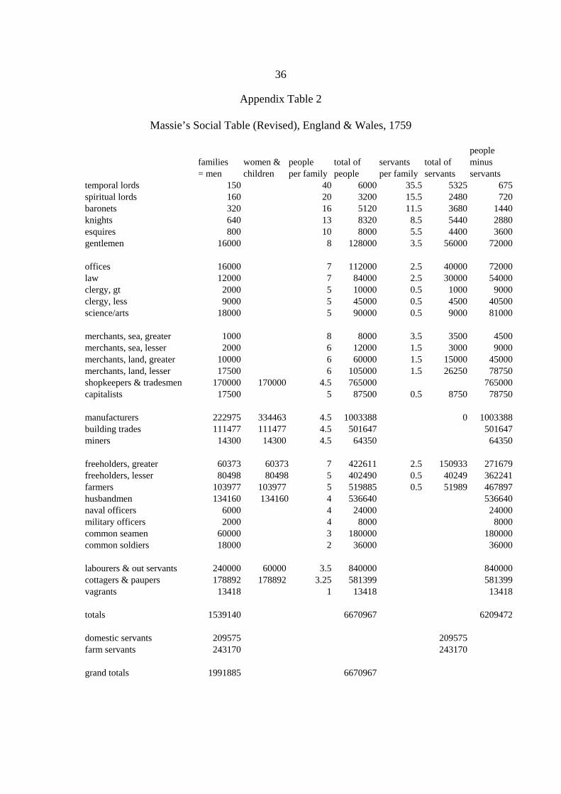
36

Appendix Table 2

Massie’s Social Table (Revised), England & Wales, 1759

peoplefamilies women & people total of servants total of minus= men children per family people per family servants servants

temporal lords 150 40 6000 35.5 5325 675 spiritual lords 160 20 3200 15.5 2480 720 baronets 320 16 5120 11.5 3680 1440 knights 640 13 8320 8.5 5440 2880 esquires 800 10 8000 5.5 4400 3600 gentlemen 16000 8 128000 3.5 56000 72000

offices 16000 7 112000 2.5 40000 72000 law 12000 7 84000 2.5 30000 54000 clergy, gt 2000 5 10000 0.5 1000 9000 clergy, less 9000 5 45000 0.5 4500 40500 science/arts 18000 5 90000 0.5 9000 81000

merchants, sea, greater 1000 8 8000 3.5 3500 4500 merchants, sea, lesser 2000 6 12000 1.5 3000 9000 merchants, land, greater 10000 6 60000 1.5 15000 45000 merchants, land, lesser 17500 6 105000 1.5 26250 78750 shopkeepers & tradesmen 170000 170000 4.5 765000 765000 capitalists 17500 5 87500 0.5 8750 78750

manufacturers 222975 334463 4.5 1003388 0 1003388 building trades 111477 111477 4.5 501647 501647 miners 14300 14300 4.5 64350 64350

freeholders, greater 60373 60373 7 422611 2.5 150933 271679 freeholders, lesser 80498 80498 5 402490 0.5 40249 362241 farmers 103977 103977 5 519885 0.5 51989 467897 husbandmen 134160 134160 4 536640 536640 naval officers 6000 4 24000 24000 military officers 2000 4 8000 8000 common seamen 60000 3 180000 180000 common soldiers 18000 2 36000 36000

labourers & out servants 240000 60000 3.5 840000 840000 cottagers & paupers 178892 178892 3.25 581399 581399 vagrants 13418 1 13418 13418

totals 1539140 6670967 6209472

domestic servants 209575 209575 farm servants 243170 243170

grand totals 1991885 6670967

37

Appendix Table 2 continued

average residualaveragenet total total net wages

familyfamily family family perincomeincome income income rents profits wages worker

temporal lords 12177 11816 1826532 1772377 1772377 spiritual lords 6088 5931 974150 948929 948929 baronets 3044 2927 974150 936725 936725 knights 1522 1436 974150 918826 918826 esquires 1218 1162 974512 929764 929764 gentlemen 472 436 7546592 6977072 6977072

offices 68 42 1084800 678000 678000 42 law 226 201 2712000 2406900 2406900 201 clergy, gt 113 108 226000 215830 215830 clergy, less 56 51 508500 462735 462735 science/arts 68 63 1220400 1128870 1128870 63

merchants, sea, greater 678 642 678000 642405 574605 67800 68 merchants, sea, lesser 452 437 904000 873490 805690 67800 34 merchants, land, greater 226 211 2260000 2107450 1429450 678000 68 merchants, land, lesser 194 178 3390000 3123037 2529787 593250 34 shopkeepers & tradesmen 51 51 8599300 8599300 2836300 5763000 17 capitalists 97 92 1700000 1611013 1017763 593250 34

manufacturers 35 35 7720289 7720289 7720289 14 building trades 29 29 3221023 3221023 3221023 14 miners 26 26 371657 371657 371657 13

freeholders, greater 115 89 6913082 5378099 3180018 1036962 1161119 10 freeholders, lesser 43 38 3456584 3047252 1590029 518488 938735 6farmers 58 53 6026301 5497578 1673973 3823606 18 husbandmen 18 18 2425613 2425613 1115782 363842 945989 4naval officers 90 90 542400 542400 542400 90 military officers 113 113 226000 226000 226000 113 common seamen 23 23 1356000 1356000 1356000 23 common soldiers 16 16 284760 284760 284760 16

labourers & outservants 20 20 4746000 4746000 4746000 16 cottagers & paupers 7 7 1313962 1313962 1313962 4 vagrants 2 2 30325 30325 30325 2

totals 75187082 70493678

domestic servants 10 2220365 2220365 farm servants 10 2473039 2473039

grand totals 75187082 75187082 19048085 12786859 43352137

factor shares 25% 17% 58%

38

Appendix Table 3

Colquhoun’s Social Table (Revised), England & Wales, 1798

peoplefamilies women & people total of servants total of minus

group = men children per family people per family servants servantspeers 287 25 7175 20.5 5884 1292 bishops 26 15 390 10.5 273 117 baronets 540 15 8100 10.5 5670 2430 knights 350 10 3500 5.5 1925 1575 esquires 6000 10 60000 5.5 33000 27000 gentlemen 20000 8 160000 3.5 70000 90000

high office 2000 7 14000 2.5 5000 9000 low office 10500 5 52500 0.5 5250 47250 eminent clergy 1000 6 6000 1.5 1500 4500 lesser clergy 10000 5 50000 0.5 5000 45000 dissenting clergy 2500 5 12500 0.5 1250 11250 lawyers 11000 5 55000 0.5 5500 49500 univ teach 500 4 2000 0 0 2000 school teach 20000 6 120000 1.5 30000 90000 liberal arts 16300 5 81500 0.5 8150 73350 theatre 1000 4 4000 0 0 4000 lunatic asylums 40 10 400 5.5 220 180

merchants, big 2000 10 20000 5.5 11000 9000 merchants, little 13000 7 91000 2.5 32500 58500 shopkeepers 74500 74500 5 372500 0.5 37250 335250 clerks 60000 60000 5 300000 0.5 30000 270000 shipowners 5000 5 25000 0.5 2500 22500 warehouse 500 6 3000 1.5 750 2250 pubs 50000 50000 5 250000 0.5 25000 225000 peddlers 800 800 5 4000 0.5 400 3600

manufacturers 25000 6 150000 1.5 37500 112500 shipbuilders 300 6 1800 1.5 450 1350 tailors, etc 25000 25000 5 125000 0.5 12500 112500 engineers 5000 5 25000 0.5 2500 22500 workers in manufacturing 445726 668589 4.5 2005767 0 0 2005767 labourers in mines 40000 40000 4.5 180000 0 0 180000

freeholders-big 40000 40000 5.5 220000 1 40000 180000 freeholders-small 120000 120000 5 600000 0.5 60000 540000 farmers 160000 160000 6 960000 1.5 240000 720000

naval officers 7000 5 35000 0.5 3500 31500 military officers 13064 5 65320 0.5 6532 58788 naval personel 52906 3 158718 0 0 158718 merchant sailors 49393 3 148179 0 0 148179 soldiers 121985 2 243970 0 0 243970

labourers in agric & females 340000 100000 4.5 1530000 0 0 1530000 paupers at work 260179 4 1040716 0 0 1040716

39

vagrants 175218 1 175218 0 0 175218 debtors 2000 5 10000 0.5 1000 9000 lunatics 2500 1 2500 0 0 2500

king 1 50 50 45.5 45.5 4.5

half pay officers 4015 5 20075 0.5 2007.5 18068 pensioned soldiers 30500 1 30500 0 30500

totals 2227630 9430378 724056.5 8706322

farm servants 340000 340000 domestic servants 384057 384057

grand totals 2951687 9430378

40

Appendix Table 3 continued

average residualaverage net total total net wagesfamily family family family per

group income income income income rents profits wages workerpeers 8000 7590 3296000 3178330 1860497 1317833 bishops 4000 3790 104000 98540 88686 9854 baronets 3000 2790 1620000 1506600 1355940 150660 knights 1500 1390 525000 486500 437850 48650 esquires 1500 1390 9000000 8340000 7506000 834000 gentlemen 700 630 15000000 13600000 11240000 2360000

high office 800 750 1600000 1500000 1500000 750 low office 200 190 2100000 1995000 1995000 190 eminent clergy 500 470 500000 470000 470000 lesser clergy 120 110 1200000 1100000 1100000 dissenting clergy 120 110 300000 275000 275000 110 lawyers 350 340 3850000 3740000 3740000 340 univ teach 600 600 300000 300000 300000 school teach 150 120 3000000 2400000 2400000 120 liberal arts 260 250 4238000 4075000 4075000 250 theatre 200 200 200000 200000 200000 200 lunatic asylums 500 390 20000 15600 15600 390

merchants, big 2600 2490 6255000 6035000 5735000 300000 150 merchants, little 800 750 11400000 10750000 8800000 1950000 150 shopkeepers 150 140 11175000 10430000 4842500 5587500 38 clerks 75 65 4500000 3900000 3900000 33 shipowners 500 490 2500000 2450000 2075000 375000 75 warehouse 800 770 400000 385000 347500 37500 75 pubs 100 90 5000000 4500000 750000 3750000 38 peddlers 40 30 32000 24000 24000 15

manufacturers 800 770 21000000 20250000 16500000 3750000 150 shipbuilders 700 670 210000 201000 156000 45000 150 tailors, etc 150 140 3750000 3500000 1625000 1875000 38 engineers 200 190 1000000 950000 950000 190 workers inmanufacturing

55 55 24514930 24514930 24514930 22

labourers in mines 40 40 1600000 1600000 1600000 20

freeholders-big 200 180 8000000 7200000 4000000 880000 2320000 29 freeholders-small 90 80 10800000 9600000 5400000 1188000 3012000 13 farmers 120 90 19200000 14400000 4224000 10176000 32

naval officers 149 139 1043000 973000 973000 139 military officers 139 129 1815896 1685256 1685256 129 naval personnel 38 38 2010428 2010428 2010428 38 merchant sailors 40 40 1975720 1975720 1975720 40 soldiers 29 29 3537565 3537565 3537565 29

labourers in agriculture 31 31 10540000 10540000 10540000 24 paupers at work 10 10 2601790 2601790 2601790 10

41

vagrants 10 10 1752180 1752180 1752180 10 debtors 45 35 90000 70000 70000 lunatics 30 30 75000 75000 75000

king 200000 199090 200000 199090 199090

half pay officers 45 35 180675 140525 140525 pensioned soldiers 20 20 610000 610000 610000

totals 204622184 190141054

farm servants 6800000 6800000 domestic servants 7681130 7681130

totals 204622184 204622184 33958063 51988997 118675124

factor shares 17% 25% 58%

42

Appendix Table 4

Smee’s data retabulated for England & Wales–men, 1846males 20 years &

overtotal working upper middlemales class working class class20 years males class paying paying& over 20 years weekly income no tax boys

& over earnings tax £50-£150 earningshillings £467/year £100/year 5s/week

trade,com, manuf 1872637 1094720 15 91393 686524 340724 farmers & graziers 242251 16123 226129 2843 agricultural labourers 826117 826117 8 167793 gardeners & florists 46550 45672 15 879 2380 nonagricul labourers 516471 516471 11 91145 army 32592 30877 5 1225 490 6744 navy & merchant 93992 92155 5 918 918 7865 professionals 53898 25500 28398 2032 other educated 87068 60061 27007 11382 govt civil servants 14274 9976 4297 234 police &parochial officers 21352 18742 15 2610 343 domestic servants 160505 160505 11 89371 independent 126996 62885 64111 5448 alms, pensions, 69469 69469 30015 residue 255744 3141255 minors 10132 168875

total 4419916 2854728 280825 1207628 3899573

43

Appendix Table 5

Smee’s data retabulated for England & Wales–women, 1846

females 20 years plustotal working

classupper middle

females females working class class other20 years 20 years class paying paying middle& over & over weekly income no tax class girls

earnings tax £50-£150 earningshillings £200/year £80/year £40/year 4s/week

trade,com, manuf 418649 321445 10 16201 81004 170540 farmers & graziers 20514 0 1244 19270 0 agricultural labourers 30161 30161 5 9839 gardeners & florists 1166 789 10 378 135 nonagricul labourers 105746 105746 7 7735 armynavy & merchantprofessionals 824 419 10 405 other educated 32164 9117 15 23047 1936 govt civil servants 551 221 15 330 15 police &parochial officers 1965 1965 7 14 domestic servants 509407 509407 11 309699 independent 329625 15 127528 86167 115930 15121 alms, pensions, 64220 64220 24837 residue 3273505 3377724

total 4788497 1043489 144972 210601 115930 3917593

44

Appendix Table 6

Smee’s incomes, England & Wales, 1846

working upper class middle pauper totalclass income class incomewages income income

trade,com, manuf 57254663 45920905 75132680 178308248 farmers & graziers 36959 7778043 24154475 31969477 agricultural labourers 19858962 19858962 gardeners & florists 1834032 118096 1952128 nonagricul labourers 17960968 17960968 army 458195 572257 49016 1079468 navy & merchant 1208103 428846 91830 1728779 professionals 37310 11908586 2872175 14818071 other educated 523667 28048546 4544440 33116654 government civil servants 11824 4659000 456133 5126957 police & parochial officers 771315 1218639 1989955 domestic servants 23140221 23140221 independent 54872795 13306105 68178900 alms, pensions, 1336890 1336890 remaining population 0 minors 2026498 3377497 5403996 other middle property 25058100 25058100

total 123096220 157434116 149160546 1336890 431027773

45

References

Afton, Bethany, and Turner, Michael, “Rent and land values,” in E.J.T. Colllins, ed.,Agrarian history of England and Wales, VII, Pt. 2 (Cambridge, 2000), pp. 1914-1939.

Allen, Robert C., "Economic structure and agricultural productivity in Europe, 1300-1800,"European Review of Economic History, 3, (2000) , pp. 1-25.

Allen, Robert C., “English and Welsh agriculture, 1300-1850: output, inputs, and income,”https://www.nuffield.ox.ac.uk/users/Allen/unpublished/AllenEandW.pdf (2005).

Allen, Robert C., “Engel’s pause: technical change, capital accumulation, and inequality inthe British industrial revolution,” Explorations in Economic History, 46, (2009), pp. 418-35.

Allen, Robert C., Bassino, J.-P., Ma, D., Moll-Murata, C., and van Zanden, J.L., “Wages,prices, and living standards in China,1739-1925: in comparison with Europe, Japan, andIndia," Economic History Review, 64, (2011), pp. 8-38.

Allen, Robert C., Murphy, T., and Schneider, E.,“The colonial origins of divergence in theAmericas: a labour market approach,” Journal of Economic History, 72, (2012), pp. 863-894.

Allen, Robert C., “American exceptionalism as a problem in global history,” Journal ofEconomic History, 74, (2014), pp. 309-350.

Allen, Robert C,. “The high wage economy and the industrial revolution: a restatement,”Economic History Review, 68, (2015), pp. 1-22.

Barnett, G.E., Two tracts by Gregory King, (Baltimore, 1936).

Baxter, R. Dudley, National income. The United Kingdom, (1868).

Beckett, J.V., “The pattern of landownership in England and Wales, 1660-1880,” EconomicHistory Review, 2nd ser., XXXVII, (1984), pp. 1-22.

Broadberry, Stephen, Campbell, B.M.S., van Leeuwen, B., “When did Britain industrialise?The sectoral distribution of the labour force and labour productivity in Britain, 1381 – 1851,”Explorations in Economic History, 50 (2013), pp. 16–27.

Broadberry, Stephen, Campbell, B.M.S., Klein, A., Overton, M., van Leeuwen, B., Britisheconomic growth: 1270-1870, (Cambridge, 2015).

Clark, Gregory, A farewell to alms: a brief economic history of the world, (Princeton, 2007).

Clark, Gregory, “National income, prices, wages, land rents, population, England,1209-1869,” http://www.econ.ucdavis.edu/faculty/gclark/data.html, (2010), accessed 2December 2015.

46

Clark, Gregory, The son also rises: surnames and the history of social mobility, (Princeton,2014).

Colquhoun, P. A treatise on indigence, (1806).

Cookson, J., ‘Political arithmetic and war in Britain, 1793-1815’, War and Society, 1 (1983),pp. 37-60.

Cooper, J.P. “The social distribution of land and men in England, 1436-1700,” EconomicHistory Review, 2nd ser., XX, (1967), pp. 419-40.

Crafts, N.F.R. "English economic growth in the eighteenth century: a re-examination ofDeane and Cole's estimates," Economic History Review, 2nd ser., XXIX, (1976).pp. 226-235.

Crafts, N.F.R., British economic growth during the industrial revolution, (Oxford, 1985)

Crafts, N.F.R. and Harley, C.K., ‘Output growth and the British industrial revolution: arestatement of the Crafts-Harley view,’ Economic History Review, XXXXV, (1992), pp. 703-30.

Deane, Phyllis, “The implications of early national income estimates for the measurement oflong-term economic growth in the United Kingdom,” Economic Development and CulturalChange, 4, (1955), pp. 3-38.

Deane, Phyllis, “Contemporary estimates of national income in the first half of thenineteenth century,” Economic History Review, 2nd ser., VIII, (1956), pp. 339-54.

Deane, Phyllis, and Cole, W.A., British economic growth: 1688-1959, (Cambridge, 1969)..

Feinstein, Charles H., Statistical tables of national income, expenditure and output of theU.K. 1855-1965, (Cambridge, 1972).

Feinstein, Charles H., “Capital formation in Great Britain,” in P. Mathias and M.M. Postan,eds., Cambridge economic history of Europe, Vol. VII, The industrial economies: capital,labour, and enterprise, Part I, Britain, France, Germany, and Scandinavia, (Cambridge,1978), pp. 28-96.

Feinstein, Charles H., “Sources and methods of estimation for domestic reproducible fixedassets, stocks and works in progress, overseas assets, and land,” in Charles H. Feinstein andSidney Pollard, eds., Studies in capital formation in the United Kingdom, 1750-1920,(Oxford, 1988), pp. 258-471.

Feinstein, Charles H., “Pessimism perpetuated: real wages and the standard of living inBritain during and after the industrial revolution,” Journal of Economic History, 58, (1988),pp.625-658.

Feinstein, Charles H., “Wage-earnings in Great Britain during the industrial revolution,” in

47

Applied economics and public policy, ed. by Iain Begg and S.G.B. Henry, (Cambridge,1988), pp. 181-208.

Floud , R., Fogel, R., Harris, B., and Hong, S.C. The changing body: health, nutrition, andhuman development in the West since 1700, (Cambridge, 2011).

Gilboy, Elizabeth W., Wages in eighteenth century England, (Cambridge, MA, 1934).

Harley, C. Knick, ”Cotton textiles and the industrial revolution: Competing Models andEvidence of Prices and Profits. (2006).”

Hollingsworth, T.H., ‘A demographic studty of the British ducal families,’ PopulationStudies, 11, (1957), pp. 4-26.

Holmes, G.S., “Gregory King and the social structure of pre-industrial England,”Transactions of the Royal Statistical Society, 5th series, 27, (1977), pp. 41-68.

Hoppit, Julian, “Political arithmetic in eighteenth-century England,” Economic HistoryReview, XXXXIX, (1996), pp. 516-40.

Hudson, Pat, The genesis of industrial capital: a study of the West Riding wool textileindustry, c. 1750-1850, (Cambridge, 1986).

Humphries, Jane. ‘The lure of aggregates and the pitfalls of the patriarchal perspective: acritique of the high wage economy interpretation of the British industrial revolution’,Economic History Review 66 (2013), pp. 693-71.

Humphries, Jane, and Schneider, Benjamin, “Spinning the industrial revolution,” OxfordUniversity, Discussion Papers in Economic and Social History, Number 145. (2016).

Humphries, Jane, and Weisdorf, Jacob, “The wages of women in England, 1260–1850,”Journal of Economic History, 75, (2015), pp. 405-447.

Innes, Joanne, “Power and happiness: empirical social enquiry in Britain, from ‘politicalarithmetic’ to ‘moral statistics,’ in Inferior Politics, (Oxford, 2009), pp. 109-175.

Kuznets, Simon, “Economic growth and income inequality,” American Economic Review,45, (1955), pp. 1-28.

Kuznets, Simon, Economic growth of nations: total output and production structure,(Cambridge, MA, 1971).

Laslett, Peter, ‘Size and structure of the household in England over three centuries,’Population Studies 23, (1969), pp. 199-223.

Linderrt, Peterr H., Baxter E&W UK 1867 (1997)http://economics.ucdavis.edu/people/fzlinder/peter-linderts-webpage/data-and-estimates/britains-social-tables-1688-on (Accessed on 22 Sept., 2017).

48

Lindert, Peter H., “Toward a comparative history of income and wealth inequality,” in Y.S.Brenner, H. Kaelble, and M. Thomas, eds., Income distribution in historical perspective,(Cambridge, 1991), pp. 212-231.

Lindert, Peter H., “When did inequality rise in Britain and America?” Journal of IncomeDistribution, 9, (2000), pp. 11-25.

Lindert, Peter H.,“Three centuries of inequality in Britain and America,” in A.B. Atkinsonand F. Bourguignon, eds, Handbook of income distribution, (Amsterdam, 2000), pp. 167-216.

Lindert, Peter H., and Williamson, Jeffrey G., "Revising England's social tables, 1688-1812," Explorations in Economic History, 19, (1982), pp. 385-408.

Lindert, Peter H., and Williamson, Jeffrey G., "Reinterpreting Britain's social tables,1688-1913," Explorations in Economic History, 20, (1983), pp. 94-109.

Lindert, Peter H., and Williamson, Jeffrey G., “English workers’ living standard during theindustrial revolution: a new look,” Economic History Review, XXXXVI, (1983), pp. 115-44.

Massie, J. A computation of the money that hath been exorbitantly raised upon the people ofGreat Britain by the sugar planters, (1760).

Mathias, Peter, “The social structure in the eighteenth century: a calculation of JosephMassie,” Economic History Review, 2nd ser., X, (1957), pp. 30-45.

Milanovic, Branko, Global inequality: a New approach for the age of globalization,(Cambridge, MA, 2016).

Milanovic, Branko, Lindert, P.H., and Williamson, J.G. (2011)., “Pre-industrial inequality,”The Economic Journal, 121, No. 551, (2011), pp. 255-272.

Mingay, G.E. English landed society in the eighteenth century, (1963).

Perkin, H., The origins of modern English society, 1780-1880, (1969).

Porter, G.R., The progress of the nation, ed. by F.W. Hirst, ( revised edition, 1912).

Smee, William Ray, The income tax, (1846).

Stephenson, Judy (2017). “‘Real’ wages? Contractors, worker, and pay in the Londonbuilding trades, 1650-1800,” The Economic History Review, forthcoming.

Thompson, F.M.L., “The social distribution of landed property in England since the sixteenthcentury,” Economic History Review, 2nd Ser., XIX, (1966), pp. 505-517

Turner, Michael, After the famine: Irish agriculture, 1850-1914, (Cambridge, 1996).

49

Wrigley, E.A., “Urban growth and agricultural change: England and the continent in theearly modern period,“ Journal of Interdisciplinary History, 15, (1985), pp. 683-728.

Wrigley, E.A. and Schofield, R.S., The population history of England, 1541-1871, (1981).

Wrigley, E.A., Davies, R.S., Oeppen, J.E., and Schofield, R.S., English population historyfrom family reconstitution, 1580-1837, (Cambridge, 1997)

Official Papers

Abstract of the Answers and Returns...for taking an account of the population; OccupationAbstract M.DCCC.XLI,. Part I. England and Wales (P.P. 1844, 587) ProQuest, U.K.Parliamentary Papers.