divider-based algorithms for hierarchical tree partitioning

Discrete Applied Mathematics 136 (2004) 227–247www.elsevier.com/locate/dam

Divider-based algorithms for hierarchical treepartitioning

Irene Finocchia ;1 , Rossella Petreschib;2

aDipartimento di Informatica, Sistemi e Produzione, Universit�a degli Studi di Roma “Tor Vergata”, Viadi Tor Vergata 110, 00133 Roma, Italy

bDipartimento di Informatica, Universit�a degli Studi di Roma “La Sapienza”, Via Salaria 113,00198 Roma, Italy

Received 30 September 2001; received in revised form 30 October 2002; accepted 19 February 2003

Abstract

We present algorithms for computing hierarchical decompositions of trees satisfying di0erentoptimization criteria, including balanced cluster size, bounded number of clusters, and logarith-mic depth of the decomposition. Furthermore, every high-level representation of the tree obtainedfrom such decompositions is guaranteed to be a tree. These criteria are relevant in many ap-plication settings, but appear to be di3cult to achieve simultaneously. Our algorithms work byvertex deletion and hinge upon the new concept of t-divider, that generalizes the well-knownconcepts of centroid and separator. The use of t-dividers, combined with a reduction to a clas-sical scheduling problem, yields an algorithm that, given a n-vertex tree T , builds in O(n log n)worst-case time a hierarchical decomposition of T satisfying all the aforementioned requirements.? 2003 Published by Elsevier B.V.

Keywords: Graph partitioning problems; Hierarchical decompositions; Trees; Centroids

1 Author partially supported by the EU under contract number IST-2001-33555 (COSIN), by the ItalianMinistry of University and Scienti@c Research (project “ALINWEB: Algorithmics for Internet and the Web”),and by the University of Rome “La Sapienza” (project for Young Researchers “Algorithms and Techniquesfor the Visualization of Large Graphs”, 2001).

2 Author partially supported by the Italian Ministry of University and Scienti@c Research (Project “AL-INWEB: Algorithmics for Internet and the Web”) and by the University of Rome “La Sapienza” (project“Parallel and Distributed Codes”, 2002).

E-mail addresses: @[email protected] (I. Finocchi), [email protected] (R. Petreschi).

0166-218X/$ - see front matter ? 2003 Published by Elsevier B.V.doi:10.1016/S0166-218X(03)00443-8

mailto:[email protected]

mailto:[email protected]

228 I. Finocchi, R. Petreschi / Discrete Applied Mathematics 136 (2004) 227–247

1. Introduction

Graphs arising in real applications are becoming increasingly large. Designing e3-cient data structures to manage them is thus an important task. A common approach tospeed up the processing of a large graph G consists of using decomposition techniquesto build a clustered graph from G: informally speaking, such a graph represents a sum-mary of G and is obtained by grouping together suitably chosen disjoint sets of vertices,called clusters, and by computing induced edges between them. Graph decompositiontechniques are often used recursively, so as to build a sequence of meta-graphs fromG: each meta-graph in the sequence is a summary of the previous one, the @rst andmore detailed meta-graph coinciding with G itself. Such a sequence de@nes a hierarchi-cal decomposition of G represented by a rooted tree, known in literature as hierarchytree, whose leaves are vertices of G and whose internal nodes are clusters. Di0erentselections of nodes of the hierarchy tree lead to di0erent high-level representations ofG that can be traversed by performing shrinks and expansions of clusters.This paper is concerned with hierarchical decompositions of trees. Tree clustering

procedures are an important subroutine for partitioning generic graphs: they can beapplied, for instance, to the block-cut-vertex tree of a graph in order to obtain a @rstrough partition of its vertices. In addition, tree-like structures frequently arise in manypractical problems (e.g., evolutionary and parse trees). A few examples of applicationsettings where recursive tree decompositions have proven to be e0ective are listed inthe following. In the @eld of dynamic graph algorithms, Frederickson’s technique formaintaining a minimum spanning tree of a graph under updates of the costs of itsedges hinges upon a multi-level topological partition of the vertices of the spanningtree useful for reducing the update time [11]. Tree layout algorithms also bene@t fromdecompositions: clusters can be visualized as single vertices or @lled-in regions, makingit possible to display e0ectively the global structure of large trees in a limited area[8]. The pro@le minimization problem, which is NP-complete on general graphs, hasbeen polynomially solved on trees thanks to a recursive partition of the vertices ofthe tree by means of centroids [15]. Other applications include parallel and distributedcomputations, operating systems, external searching, allocation of service centers; werefer the interested reader to [2,3,7,14] for more details on these topics.According to the application at hand, di0erent optimization criteria can be consid-

ered when building clusters. It is in general well accepted that good decompositionsshould exhibit a strong relationship between vertices in the same cluster and a lowcoupling between clusters. Additional objective functions should be optimized whendealing with recursive partitions. Among them, structural properties of the hierarchytree such as limited degree, small depth, and balancing deserve special attention. Forinstance, in a distributed setting, where clusters correspond to processors and verticesto tasks to be performed, having a bounded number of clusters of almost equal sizeenhances locality, decreases communication, and guarantees better load balancing. Fi-nally, it is quite natural to require any high-level representation of a graph obtainedfrom its hierarchy tree to reNect the topology and the properties of the graph itself.An immediate motivation for this comes from graph drawing applications: in order notto mislead the viewer, it is desirable, e.g., for any representation of a planar graph to

I. Finocchi, R. Petreschi / Discrete Applied Mathematics 136 (2004) 227–247 229

be planar or for any representation of a tree to be connected and acyclic. A hierarchytree that satis@es this property is said to be valid [9]. Building valid hierarchy treesor checking the validity of a given hierarchy tree in polynomial time may be quitedi3cult.

1.1. Related work

Due to the special structure of trees, most graph partitioning algorithms either are note3cient or fail to @nd appropriate tree decompositions. For this reason a lot of researchhas been devoted since the 1980s to designing speci@c tree partitioning algorithmstailored to a variety of applications (see, e.g., [2,4,7,14,17,19,21] and the referencestherein). Independently of the optimized objective function, we can roughly distinguishtwo main approaches to tree partitioning, according to the fact that clusters are obtainedby deleting vertices or edges.A well-known technique based on edge deletion, the shifting algorithm technique,

has been presented in [19] and applied to many optimization problems on trees inseveral subsequent papers [1–3,20]. A partition of a tree is identi@ed by associatingcuts to its edges. Cuts are assigned via a sequence of shifts, i.e., basic operations thatmove a cut from an edge to an adjacent one; di0erent shifting rules allow it to optimizedi0erent functions. Other edge deletion algorithms for tree partitioning are describedin [4,14]. In particular, [14] suggests algorithms for partitioning a n-vertex tree into gbalanced clusters: the size of each cluster is in the range [(1 − �=2)n=g, (1 + �)n=g],where parameter �∈ [0; 1] can be given as input.At @rst sight, removing vertices may appear to be less Nexible than removing edges:

based on the degree of the deleted vertex, the tree may be disconnected into severalsubtrees of very di0erent size, and optimizing both cluster size and number of subtreesmay be more di3cult. However, an accurate choice of the vertex to be removed (e.g.,choosing a centroid or a center of the tree) allows it to guarantee upper/lower boundson the size or on the diameter of each cluster. An example can be found in [15].To conclude, we remark that most of the aforementioned algorithms may not be good

at optimizing simultaneously properties of the hierarchy tree such as balancing, depth,and degree. Moreover, since typically they are not applied recursively, they do notaddress at all the problem of building valid hierarchy trees: actually, it is not di3cultto see that many of the partitioning algorithms that @nd disconnected clusters (such asthe algorithms in [14]) may produce non-valid decompositions.

1.2. Results and techniques

In this paper we consider the problem of computing hierarchical decompositionsof trees that: (1) are valid; (2) have logarithmic depth; (3) exhibit balanced clustersize; and (4) have bounded degree. We present e3cient algorithms based on vertexdeletion for computing such decompositions. We @rst show that it is easy to guaranteeeither logarithmic depth or bounded degree for the hierarchy tree, but not both, exceptfor special classes of trees. We therefore present an algorithm that overcomes thisdrawback: if n is the number of vertices of the original tree, it builds in O(n log n)


worst-case running time hierarchy trees that exhibit limited degree, balanced clustersize, logarithmic depth, and are valid. We remark that P(n) is a trivial lower boundon the construction of any hierarchy tree.The backbone of our algorithms is the new concept of t-divider, that generalizes

concepts well known in literature, such as centroids and separators [6,16,18]. Theperformances of the almost-optimal partitioning algorithm are achieved by exploitingthe use of t-dividers, a reduction to a classical scheduling problem, and the followingsimple idea: when the degree of the hierarchy tree must be limited by a constant, smalldepth and balanced cluster size can be more easily guaranteed if clusters coveringnon-connected subgraphs are allowed. In order to preserve the structure of the originaltree T in the decomposition, we consider a “weak” form of connectivity relaxation,forcing clusters to satisfy a short distance property: for each pair of disconnectedcomponents in the same cluster there exist two representative vertices whose distancein T is 2. Roughly speaking, the short distance property makes “unnatural” partitionsof the tree not possible and allows us to prove that the algorithm builds valid hierarchytrees.

1.3. Structure of the paper

Section 2 recalls terminology and preliminary de@nitions related to hierarchy trees.Section 3 introduces the notion of t-divider of a tree, providing a structural charac-terization of the set of t-dividers. Section 4 presents two naQRve partitioning strategiesand discusses their drawbacks. Section 5 describes the improved scheduling-based al-gorithm, analyzing its performances. Section 6 sums up and addresses directions forfurther research.

2. Background on hierarchy trees

In this section we give preliminary de@nitions and notation used throughout the paper.In particular, we recall the de@nition of hierarchy tree and we discuss the concepts ofcovering and of contraction of a graph on a hierarchy tree associated with it [5,9].

De�nition 1. A hierarchy tree HT (N; A) associated with a graph G(V; E) is a rootedtree whose set of leaves coincides with the set of vertices of G.

According to standard terminology, we call depth of HT the maximum distance froma leaf to the root and degree of a node of HT the number of its children. W.l.o.g. weconsider hierarchy trees whose internal nodes have degree ¿ 1.

Each node c∈N represents a cluster of vertices of G, that we call vertices coveredby c. Namely, each leaf in HT covers a single vertex of G and each internal node ccovers all the vertices covered by its children, i.e., all the leaves in the subtree rootedat c. For brevity, we write u ≺ c to indicate that a vertex u∈V is covered by a clusterc∈N . The cardinality of a cluster c is the number of vertices covered by c. We say


that c is a singleton if its cardinality is equal to 1. For any c∈N , we denote by S(c)the subgraph of G induced by the vertices covered by c.

Two clusters c and c′ which are neither coincident nor ancestors of each other areconnected by a link if there exists at least an edge e = (u; v)∈E such that u ≺ c andv ≺ c′ in HT ; if more than one edge of this kind exists, we consider only a singlelink. We denote by L the set of all such links. Given a subset N ′ of nodes of HT ,the graph induced by N ′ is the graph G′(N ′; L′), where L′ contains all the links ofL whose endpoints are in N ′. From the above de@nitions it follows that G′ containsneither self-loops nor multiple edges.

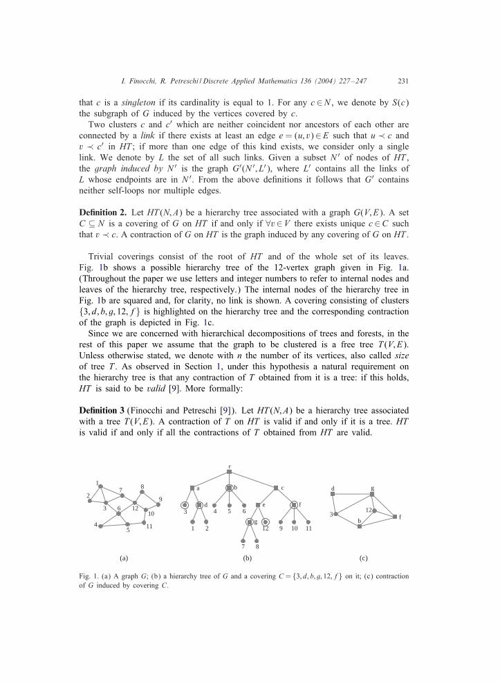
De�nition 2. Let HT (N; A) be a hierarchy tree associated with a graph G(V; E). A setC ⊆ N is a covering of G on HT if and only if ∀v∈V there exists unique c∈C suchthat v ≺ c. A contraction of G on HT is the graph induced by any covering of G on HT .

Trivial coverings consist of the root of HT and of the whole set of its leaves.Fig. 1b shows a possible hierarchy tree of the 12-vertex graph given in Fig. 1a.(Throughout the paper we use letters and integer numbers to refer to internal nodes andleaves of the hierarchy tree, respectively.) The internal nodes of the hierarchy tree inFig. 1b are squared and, for clarity, no link is shown. A covering consisting of clusters{3; d; b; g; 12; f} is highlighted on the hierarchy tree and the corresponding contractionof the graph is depicted in Fig. 1c.Since we are concerned with hierarchical decompositions of trees and forests, in the

rest of this paper we assume that the graph to be clustered is a free tree T (V; E).Unless otherwise stated, we denote with n the number of its vertices, also called sizeof tree T . As observed in Section 1, under this hypothesis a natural requirement onthe hierarchy tree is that any contraction of T obtained from it is a tree: if this holds,HT is said to be valid [9]. More formally:

De�nition 3 (Finocchi and Petreschi [9]). Let HT (N; A) be a hierarchy tree associatedwith a tree T (V; E). A contraction of T on HT is valid if and only if it is a tree. HTis valid if and only if all the contractions of T obtained from HT are valid.

1 2

3 4 5 6

7 8

12 9 10 11

r

a b c

d e f

g

(b) (c)

d

312

g

fb

(a)

1

2

3

78

9

11

106

45

12

Fig. 1. (a) A graph G; (b) a hierarchy tree of G and a covering C = {3; d; b; g; 12; f} on it; (c) contractionof G induced by covering C.


(d)(b)(a) (c) (e)

r

2 3a

41

1 2 3 4 a 3 4 2a 3

r

3 4a

21

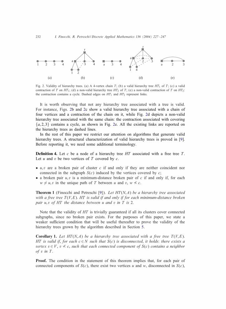
Fig. 2. Validity of hierarchy trees. (a) A 4-vertex chain T ; (b) a valid hierarchy tree HT1 of T ; (c) a validcontraction of T on HT1; (d) a non-valid hierarchy tree HT2 of T ; (e) a non-valid contraction of T on HT2:the contraction contains a cycle. Dashed edges on HT1 and HT2 represent links.

It is worth observing that not any hierarchy tree associated with a tree is valid.For instance, Figs. 2b and 2c show a valid hierarchy tree associated with a chain offour vertices and a contraction of the chain on it, while Fig. 2d depicts a non-validhierarchy tree associated with the same chain: the contraction associated with covering{a; 2; 3} contains a cycle, as shown in Fig. 2e. All the existing links are reported onthe hierarchy trees as dashed lines.In the rest of this paper we restrict our attention on algorithms that generate valid

hierarchy trees. A structural characterization of valid hierarchy trees is proved in [9].Before reporting it, we need some additional terminology.

De�nition 4. Let c be a node of a hierarchy tree HT associated with a free tree T .Let u and v be two vertices of T covered by c.

• u; v are a broken pair of cluster c if and only if they are neither coincident norconnected in the subgraph S(c) induced by the vertices covered by c;

• a broken pair u; v is a minimum-distance broken pair of c if and only if, for eachw = u; v in the unique path of T between u and v, w � c.

Theorem 1 (Finocchi and Petreschi [9]). Let HT (N; A) be a hierarchy tree associatedwith a free tree T (V; E). HT is valid if and only if for each minimum-distance brokenpair u; v of HT the distance between u and v in T is 2.

Note that the validity of HT is trivially guaranteed if all its clusters cover connectedsubgraphs, since no broken pair exists. For the purposes of this paper, we state aweaker su3cient condition that will be useful thereafter to prove the validity of thehierarchy trees grown by the algorithm described in Section 5.

Corollary 1. Let HT (N; A) be a hierarchy tree associated with a free tree T (V; E).HT is valid if, for each c∈N such that S(c) is disconnected, it holds: there exists avertex v∈V , v � c, such that each connected component of S(c) contains a neighborof v in T .

Proof. The condition in the statement of this theorem implies that, for each pair ofconnected components of S(c), there exist two vertices u and w, disconnected in S(c),


whose distance in T is 2: actually, u and w are neighbors of vertex v in T . Hence, thecondition in the statement of Theorem 1 holds and the hierarchy tree is valid.

3. Properties of t-dividers

In this section we introduce the concept of t-divider of trees and forests: t-dividersgeneralize the well-known concepts of centroid and separator and are the backbone ofthe tree decomposition algorithms presented in Sections 4 and 5.

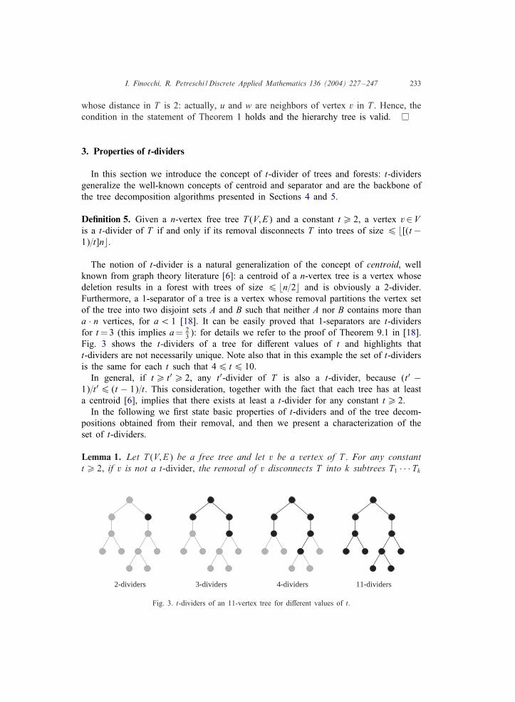
De�nition 5. Given a n-vertex free tree T (V; E) and a constant t¿ 2, a vertex v∈Vis a t-divider of T if and only if its removal disconnects T into trees of size 6 [(t −1)=t]n�.

The notion of t-divider is a natural generalization of the concept of centroid, wellknown from graph theory literature [6]: a centroid of a n-vertex tree is a vertex whosedeletion results in a forest with trees of size 6 n=2� and is obviously a 2-divider.Furthermore, a 1-separator of a tree is a vertex whose removal partitions the vertex setof the tree into two disjoint sets A and B such that neither A nor B contains more thana · n vertices, for a ¡ 1 [18]. It can be easily proved that 1-separators are t-dividersfor t =3 (this implies a= 2

3): for details we refer to the proof of Theorem 9.1 in [18].Fig. 3 shows the t-dividers of a tree for di0erent values of t and highlights thatt-dividers are not necessarily unique. Note also that in this example the set of t-dividersis the same for each t such that 46 t6 10.

In general, if t¿ t′¿ 2, any t′-divider of T is also a t-divider, because (t′ −1)=t′6 (t − 1)=t. This consideration, together with the fact that each tree has at leasta centroid [6], implies that there exists at least a t-divider for any constant t¿ 2.

In the following we @rst state basic properties of t-dividers and of the tree decom-positions obtained from their removal, and then we present a characterization of theset of t-dividers.

Lemma 1. Let T (V; E) be a free tree and let v be a vertex of T . For any constantt¿ 2, if v is not a t-divider, the removal of v disconnects T into k subtrees T1 · · ·Tk

2-dividers 3-dividers 4-dividers 11-dividers

Fig. 3. t-dividers of an 11-vertex tree for di0erent values of t.


such that, ∀j ∈ [1; k], size(Tj) = [(t − 1)=t]n� and there exists a unique Ti with morethan [(t − 1)=t]n� vertices.

Proof. As v is not a t-divider, at least a tree among T1 · · ·Tk , say Ti, must have size¿ [(t−1)=t]n�. The number of all the vertices of T di0erent from v and ∈ Ti is equalto n − size(Ti)− 1¡ n − [(t − 1)=t]n� − 16 n=t� − 16 n=t�6 [(t − 1)=t]n�, sincet¿ 2. Hence, any subtree other than Ti has size ¡ [(t − 1)=t]n�. This proves that Ti

is unique.

Lemma 2. Let T (V; E) be a free tree and let v be a vertex of V whose removal dis-connects T into k subtrees T1 · · ·Tk . Let t¿ 2 be a constant and let h be the numberof subtrees among T1 · · ·Tk with size equal to [(t − 1)=t]n�. Then 06 h6 2 andt ¿ 2 ⇒ h6 1.

Proof. The following inequality must hold: h[(t−1)=t]n�+16 n. The most favorablescenario is when [(t − 1)=t]n� is minimum, i.e., for t = 2. In this case the inequalityyields n=2�6 (n−1)=h. Assuming h ¿ 2 implies n=2�¡ (n−1)=2, that is impossible.Hence, it must be h6 2.

Let us now assume h=2. Since [(t−1)=t]n�=[(t−1)=t]n−�, 06 � ¡ 1, we musthave [(t − 1)=t]n6 (n − 1)=2 + � ¡ (n + 1)=2. By means of simple manipulations it iseasy to see that this is equivalent to require t ¡ 2n=(n−1). The case n=2 is impossible,because we have a vertex and at least two non empty trees, and for n ¿ 2 it holds2n=(n− 1)6 3. Thus, h=2 is possible only if t ¡ 3, proving that t ¿ 2 ⇒ h6 1.

Theorem 2. Let T (V; E) be a free tree and let v be a vertex of V whose removaldisconnects T into k subtrees T1 · · ·Tk . Let t¿ 2 be a constant. Then:

1. if v is not a t-divider, all the t-dividers of T are in the maximum size subtreeamong T1 · · ·Tk ;

2. if v is a t-divider, let h be the number of subtrees among T1 · · ·Tk of size equalto [(t − 1)=t]n�. Then:(a) h = 2 ⇒ T contains no other t-divider;(b) h = 1 ⇒ all the other t-dividers of T , if any, are in the unique subtree of

size [(t − 1)=t]n�;(c) h=0 ⇒ all the other t-dividers of T , if any, are in subtrees of size ¿ n=t�.

Proof. Let us @rst consider the case where v is not a t-divider. In view of Lemma 1there exists a unique Ti among T1 · · ·Tk with more than [(t − 1)=t]n� vertices. Let wbe any t-divider of T . Then w must belong to Ti: if w∈Tj, j = i, its removal from Twould generate the subtree containing Ti, which has size ¿ [(t−1)=t]n�, contradictingthe fact that w is a t-divider.Let us now assume that v is a t-divider. In view of Lemma 2, 06 h6 2. If h¿ 1,

i.e., there exists at least a tree Ti of size equal to [(t−1)=t]n�, then each subtree otherthan Ti does not contain t-dividers, because the removal of any of its vertices wouldgenerate a tree - including both v and Ti - of size at least size(Ti)+1¿ [(t − 1)=t]n�.


di dju

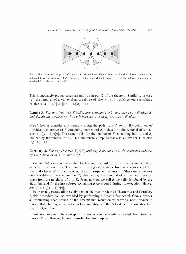
Fig. 4. Illustration of the proof of Lemma 3. Dashed lines delimit from the left the subtree containing dj

obtained from the removal of di . Similarly, dotted lines delimit from the right the subtree containing di

obtained from the removal of dj .

This immediately proves cases (a) and (b) in part 2 of the theorem. Similarly, in case(c), the removal of a vertex from a subtree of size ¡ n=t� would generate a subtreeof size ¿ n − n=t�¿ [(t − 1)=t]n�.

Lemma 3. For any free tree T (V; E), any constant t¿ 2, and any two t-dividers di

and dj, all the vertices on the path between di and dj are also t-dividers.

Proof. Let us consider any vertex u along the path from di to dj. By de@nition oft-divider, the subtree of T containing both u and dj induced by the removal of di hassize 6 [(t − 1)=t]n�. The same holds for the subtree of T containing both u and di

induced by the removal of dj. This immediately implies that u is a t-divider. (See alsoFig. 4.)

Corollary 2. For any free tree T (V; E) and any constant t¿ 2, the subgraph inducedby the t-dividers of T is connected.

Finding t-dividers. An algorithm for @nding a t-divider of a tree can be immediatelyderived from case 1 of Theorem 2. The algorithm starts from any vertex v of thetree and checks if v is a t-divider. If so, it stops and returns v. Otherwise, it iterateson the subtree of maximum size Ti obtained by the removal of v; the new iterationstarts from the neighbor of v in Ti. From now on we call d the t-divider found by thealgorithm and Td the last subtree containing d considered during its execution. Hence,size(Td)¿ [(t − 1)=t]n�.

In order to generate all the t-dividers of the tree, in view of Theorem 2 and Corollary2, this procedure can be extended by performing a breadth-@rst search from t-dividerd, terminating each branch of the breadth-@rst recursion whenever a non-t-divider isfound. Both @nding a t-divider and enumerating all the t-dividers of a n-vertex treerequire O(n) time.

t-divided forests. The concept of t-divider can be easily extended from trees toforests. The following lemma is useful for this purpose:


Lemma 4. Let F be a forest of T1 · · ·Th free trees and let t¿ 2 be a constant. Ifwe denote by f the size of the forest, i.e., f =

∑hi=1 size(Ti), then at most one tree

has size ¿ [(t − 1)=t]f�.

Proof. Let us suppose that there exists a tree Ti such that size(Ti)¿ [(t − 1)=t]f�.Then:

06h∑

j=1; j �=i

size(Tj) = f − size(Ti)6f −⌊

t − 1t

f⌋− 16

⌈ft

⌉− 1

6⌊

ft

⌋6

⌊t − 1

tf⌋

since t¿ 2. This implies the uniqueness of Ti, if it exists.

We call a f-vertex forest F t-divided if and only if all its trees have size 6 [(t −1)=t]f�. Given a forest F, in view of Lemma 4 only two cases are possible: either Fis already t-divided or it can be t-divided by removing a single vertex, that we willcall t-divider for F. This vertex must be searched in the maximum size tree of F,say Ti, and any t-divider of Ti is also a t-divider for F. We remark that it may alsoexist a vertex v∈Ti that is a t-divider for F but not for Ti.

4. Na'(ve decomposition approaches

In order to grow a hierarchy tree out of a graph, a simple top-down strategy works asfollows: starting from the root of the hierarchy tree, which is a contraction of the wholegraph, the vertices of the graph are partitioned by means of a clustering subroutineand the clusters children of the root (at least 2) are generated. The procedure is thenrecursively applied on all these clusters. It is obvious that very di0erent hierarchy treescan be associated with the same graph, depending on the clustering algorithm used assubroutine.In this section we devise two clustering algorithms for partitioning a n-vertex tree

T . Both algorithms are extremely simple and hinge upon the concept of t-divider.Their analyses suggest that it is easy to guarantee either logarithmic depth or boundeddegree for the hierarchy tree, but not both, except for special classes of trees. Thismotivates the design of the more sophisticated scheduling-based algorithm presented inSection 5.Though the de@nition of t-divider holds both on free and on rooted trees, in the

course of the presentation we assume that T has been rooted at a vertex r. We focuson a generic step during the top-down construction of the hierarchy tree HT and wecall c the node of HT considered at that step. Unless otherwise stated, we assume thatthe subgraph to be clustered S(c) is a tree named Tc and having size nc.


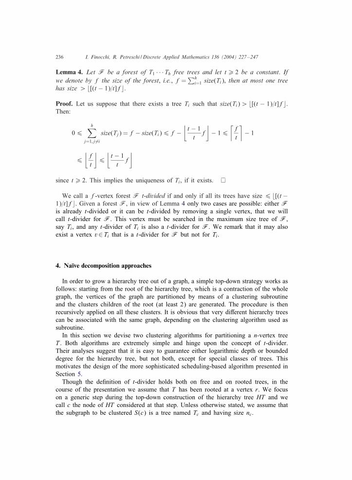
Fig. 5. Tree partitions obtained by the naQRve algorithms: subtrees assigned to the same cluster are @lled inwith the same color and pattern, and edges joining vertices in di0erent clusters are dashed. (a) Centroid d andsubtree sizes of the tree; (b) partition computed by algorithm SimpleClustering; (c) partition computedby algorithm ConnectedClustering for g = 3.

4.1. Hierarchy trees of logarithmic depth

A straightforward application of the concept of t-divider leads to the following al-gorithm:

Algorithm SimpleClustering(Tc; t). After a t-divider of Tc has been found, considerthe k subtrees T1 · · ·Tk obtained from Tc by removing the t-divider d and create kchildren c1 · · · ck of node c in the hierarchy tree: ∀i∈ [1; k] child ci covers the verticesin subtree Ti. The t-divider d is added back to the cluster having minimum cardinality.(See Fig. 5b.)

As the cardinality of each new cluster is upper bounded by [(t−1)=t]nc�, the hierarchytree HT computed by recursively applying algorithm SimpleClustering has depthO(log n). Moreover, let u be any vertex of the original tree T and let cu be thesingleton of HT associated with vertex u: during the construction of HT u is visitedin total as many times as the depth of node cu in HT, thus giving worst-case runningtime O(n log n) to build the entire hierarchy tree.It is also worth observing that the subgraph induced by the vertices covered by

every cluster in the hierarchy tree is connected. From now on, where there is noambiguity we refer to this property as connectivity of clusters. As observed in Section2, hierarchy trees whose clusters are connected are always valid. The stated propertiescan be resumed as follows:

Remark 1. Let T (V; E) be a n-vertex free tree and let $ be its maximum degree.Algorithm SimpleClustering computes a valid hierarchy tree of T having depthO(log n) and degree 6$ in O(n log n) worst-case running time.


(b)

(a)

(c)0 1

10

9

8

7

6

5

4

3

2

j

i

h

g

f

e

d

c

b

a

0

1

10

98765432b

a

0 110 9 83

7 62jih 5 4

gfed

cb

a

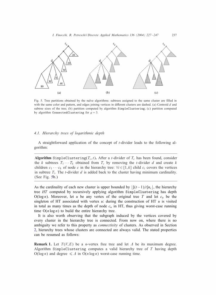
Fig. 6. Di0erent hierarchy trees associated by di0erent clustering algorithms with an 11-vertex star centeredat vertex 0: (a) SimpleClustering; (b) ConnectedClustering for g=2; (c) BalancedClustering forg = 2.

Even if algorithm SimpleClustering can be implemented using o0 the shelf datastructures and generates hierarchy trees with small depth, the structure of the returnedhierarchy tree HT may be irregular and may depend too much on the input tree:namely, the degree of the internal nodes of HT may be too large, since it dependson the degree of the t-divider found by the algorithm at each step. For instance, thehierarchy tree shown in Fig. 6a is obtained running algorithm SimpleClustering onan 11-vertex star centered at vertex 0.

4.2. Hierarchy trees of bounded degree

In order to generate hierarchy trees with bounded degree g¿ 2 we can re@ne thenaQRve approach as follows:

Algorithm ConnectedClustering(Tc; g; t). After a t-divider of Tc has been found,consider the k subtrees T1 · · ·Tk obtained from Tc by removing the t-divider d andcheck the value k. If k6 g, work exactly as in algorithm SimpleClustering. Other-wise, sort the subtrees in non-increasing order by size: w.l.o.g. let T1 · · ·Tg · · ·Tk be thesorted sequence. Create g children c1 · · · cg of node c in the hierarchy tree: ∀i∈ [1; g−1]; ci covers the vertices in subtree Ti and cg covers the vertices of T ′={d}∪⋃k

h=g Th.(See Fig. 5c.)

It is easy to see that T ′ is connected thanks to the presence of the t-divider d andthat the degree of HT is at most g (it could be smaller than g due to the case k6 g).Nothing is guaranteed about the size of T ′: HT may be therefore very unbalanced upto reach linear height (see Fig. 6b).


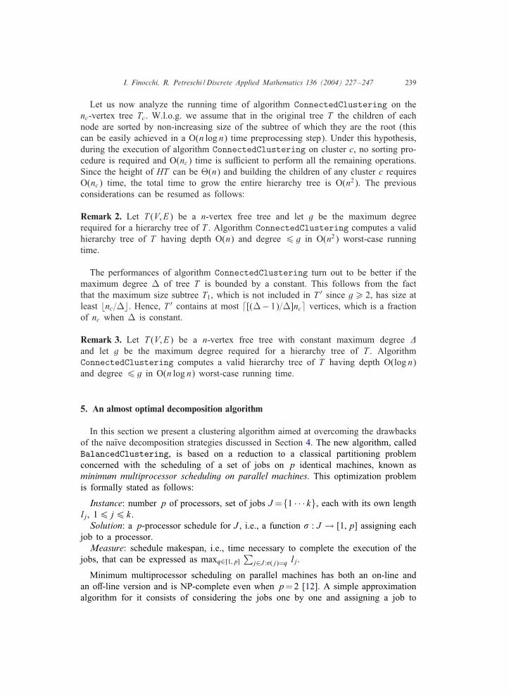
Let us now analyze the running time of algorithm ConnectedClustering on thenc-vertex tree Tc. W.l.o.g. we assume that in the original tree T the children of eachnode are sorted by non-increasing size of the subtree of which they are the root (thiscan be easily achieved in a O(n log n) time preprocessing step). Under this hypothesis,during the execution of algorithm ConnectedClustering on cluster c, no sorting pro-cedure is required and O(nc) time is su3cient to perform all the remaining operations.Since the height of HT can be T(n) and building the children of any cluster c requiresO(nc) time, the total time to grow the entire hierarchy tree is O(n2). The previousconsiderations can be resumed as follows:

Remark 2. Let T (V; E) be a n-vertex free tree and let g be the maximum degreerequired for a hierarchy tree of T . Algorithm ConnectedClustering computes a validhierarchy tree of T having depth O(n) and degree 6 g in O(n2) worst-case runningtime.

The performances of algorithm ConnectedClustering turn out to be better if themaximum degree U of tree T is bounded by a constant. This follows from the factthat the maximum size subtree T1, which is not included in T ′ since g¿ 2, has size atleast nc=U�. Hence, T ′ contains at most [(U−1)=U]nc� vertices, which is a fractionof nc when U is constant.

Remark 3. Let T (V; E) be a n-vertex free tree with constant maximum degree $and let g be the maximum degree required for a hierarchy tree of T . AlgorithmConnectedClustering computes a valid hierarchy tree of T having depth O(log n)and degree 6 g in O(n log n) worst-case running time.

5. An almost optimal decomposition algorithm

In this section we present a clustering algorithm aimed at overcoming the drawbacksof the naQRve decomposition strategies discussed in Section 4. The new algorithm, calledBalancedClustering, is based on a reduction to a classical partitioning problemconcerned with the scheduling of a set of jobs on p identical machines, known asminimum multiprocessor scheduling on parallel machines. This optimization problemis formally stated as follows:

Instance: number p of processors, set of jobs J ={1 · · · k}, each with its own lengthlj, 16 j6 k.

Solution: a p-processor schedule for J , i.e., a function ( : J → [1; p] assigning eachjob to a processor.Measure: schedule makespan, i.e., time necessary to complete the execution of the

jobs, that can be expressed as maxq∈[1;p]∑

j∈J :(( j)=q lj.

Minimum multiprocessor scheduling on parallel machines has both an on-line andan o0-line version and is NP-complete even when p=2 [12]. A simple approximationalgorithm for it consists of considering the jobs one by one and assigning a job to


Fig. 7. Algorithm BalancedClustering.

the machine currently having the smallest load [13]. From now on we will refer tothis subroutine as GrahamSchedule. In the o0-line case, very good solutions (i.e.,approximation ratio 4

3 − 1=3p) can be obtained if the jobs are previously sorted innon-increasing order by length, so as to consider longer jobs @rst.Let us now come back to the tree partitioning problem. We assume that the degree

of the hierarchy tree should be limited by a constant g¿ 2 that algorithm Balanced-Clustering receives as input. Under this assumption, we exploit the idea that thebalancing of the structure of the hierarchy tree can be best preserved if clusters coveringnon-connected subgraphs are allowed: in other words, if one is willing to give up theproperty of connectivity, we expect that more balanced hierarchy trees can be built.On the other side, if clusters are allowed to be non-connected, special attention mustbe paid to guarantee the validity of the hierarchy tree.Since we admit the existence of non-connected clusters, in the rest of this section

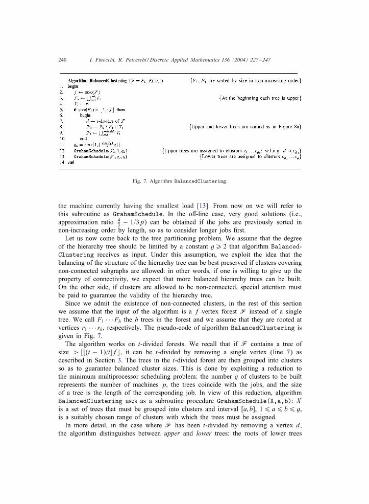
we assume that the input of the algorithm is a f-vertex forest F instead of a singletree. We call F1 · · ·Fh the h trees in the forest and we assume that they are rooted atvertices r1 · · · rh, respectively. The pseudo-code of algorithm BalancedClustering isgiven in Fig. 7.The algorithm works on t-divided forests. We recall that if F contains a tree of

size ¿ [(t − 1)=t]f�, it can be t-divided by removing a single vertex (line 7) asdescribed in Section 3. The trees in the t-divided forest are then grouped into clustersso as to guarantee balanced cluster sizes. This is done by exploiting a reduction tothe minimum multiprocessor scheduling problem: the number g of clusters to be builtrepresents the number of machines p, the trees coincide with the jobs, and the sizeof a tree is the length of the corresponding job. In view of this reduction, algorithmBalancedClustering uses as a subroutine procedure GrahamSchedule(X,a,b): Xis a set of trees that must be grouped into clusters and interval [a; b], 16 a6 b6 g,is a suitably chosen range of clusters with which the trees must be assigned.In more detail, in the case where F has been t-divided by removing a vertex d,

the algorithm distinguishes between upper and lower trees: the roots of lower trees


(a)

c

c'v

...

...

ℑForest

d

T2

T3 Tq

T1

r1

...

F2Fh

rhr2

x

(b)

c1 c2

ℑ { }

c

c'v

T2F2 U T2F2 ,

link induced by edge (r2,v)

link induced by edge (x,d)

link induced by edge (r1,v)

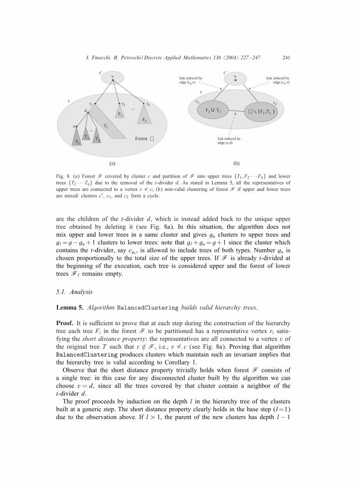
Fig. 8. (a) Forest F covered by cluster c and partition of F into upper trees {T1; F2 · · ·Fh} and lowertrees {T2 · · · Tq} due to the removal of the t-divider d. As stated in Lemma 5, all the representatives ofupper trees are connected to a vertex v � c; (b) non-valid clustering of forest F if upper and lower treesare mixed: clusters c′, c1, and c2 form a cycle.

are the children of the t-divider d, which is instead added back to the unique uppertree obtained by deleting it (see Fig. 8a). In this situation, the algorithm does notmix upper and lower trees in a same cluster and gives gu clusters to upper trees andgl = g− gu +1 clusters to lower trees: note that gl + gu = g+1 since the cluster whichcontains the t-divider, say cgu , is allowed to include trees of both types. Number gu ischosen proportionally to the total size of the upper trees. If F is already t-divided atthe beginning of the execution, each tree is considered upper and the forest of lowertrees Fl remains empty.

5.1. Analysis

Lemma 5. Algorithm BalancedClustering builds valid hierarchy trees.

Proof. It is su3cient to prove that at each step during the construction of the hierarchytree each tree Fi in the forest F to be partitioned has a representative vertex ri satis-fying the short distance property: the representatives are all connected to a vertex v ofthe original tree T such that v ∈ F, i.e., v � c (see Fig. 8a). Proving that algorithmBalancedClustering produces clusters which maintain such an invariant implies thatthe hierarchy tree is valid according to Corollary 1.Observe that the short distance property trivially holds when forest F consists of

a single tree: in this case for any disconnected cluster built by the algorithm we canchoose v = d, since all the trees covered by that cluster contain a neighbor of thet-divider d.The proof proceeds by induction on the depth l in the hierarchy tree of the clusters

built at a generic step. The short distance property clearly holds in the base step (l=1)due to the observation above. If l ¿ 1, the parent of the new clusters has depth l − 1


and by inductive hypothesis satis@es the property, as illustrated in Fig. 8a. As far as Fis partitioned, the invariant is maintained both by clusters containing upper trees andby clusters consisting only of lower trees: this follows from the inductive hypothesisin the former case and can be easily proved choosing v = d in the latter.

It is worth remarking the importance of the distinction between upper and lowertrees for obtaining a valid decomposition. Indeed, Fig. 8b shows that arbitrarily mixingupper and lower trees in the same cluster may produce non valid partitions: in theexample, where the upper tree F2 and the lower tree T2 are covered by cluster c1 andall the other trees are covered by c2, a non-valid view is obtained as proved by theexistence of cycle ¡ c1; c2; c′; c1 ¿.In the following we study the running time of algorithm BalancedClustering and

the structural properties of the hierarchy trees that it builds. Some preliminary lemmaswill be useful at this aim.

Lemma 6. If F is not t-divided at the beginning of the execution of algorithmBalancedClustering, then size(Fu)6 f=t�6 [(t − 1)=t]f�6 size(Fl) after theassignments in lines 8 and 9.

Proof. As far as the algorithm for @nding t-dividers is concerned, d is the @rst t-dividerof F encountered along the path from r1 to d. Hence, the size of the subtree of F1

rooted at d is ¿ [(t−1)=t]f�. This implies that size(Fu)6 f=t� after the assignmentstatement in line 8 of Figure 7. The inequality [(t − 1)=t]f�6 size(Fl) immediatelyfollows since Fl =F \Fu.

Corollary 3. If F is not t-divided at the beginning of the execution of algorithmBalancedClustering, then 16 gu ¡ gl6 g.

Proof. Recall that gl = g − gu + 1 and that gu is chosen proportionally to size(Fu)(see line 11 in Fig. 7). Lemma 6 completes the proof.

The next two lemmas prove that algorithm BalancedClustering @nds balancedpartitions. Both the use of t-dividers and the choice of the scheduling subroutine arecrucial in the proofs.

Lemma 7. Let F be a f-vertex forest and let t¿ 2 and g¿ 2 be two constants. Letc1 · · · cg be the clusters built by algorithm BalancedClustering (F; g; t) and lets1 · · · sg be their cardinalities. If F is not t-divided at the beginning of the executionof the algorithm, then, ∀i; j such that i; j ∈ [1; gu − 1] or i; j ∈ [gu; g], |si − sj|6 [(t −1)=t]f�.

Proof. Let us @rst consider a generic pair of clusters built by algorithm Balanced-Clustering, say ci and cj, such that gu6 i ¡ j6 g. Consider a generic step kduring the execution of procedure GrahamSchedule in line 13 of algorithm Balanced-Clustering. As far as the algorithm is concerned, both clusters ci and cj are used by


(a)

ci cj

nk

(b)

ci cj

nk

(c)

ci cj

nkks iksj

ks iks j ks i

ksj

Fig. 9. Illustration of the proof of Lemma 7.

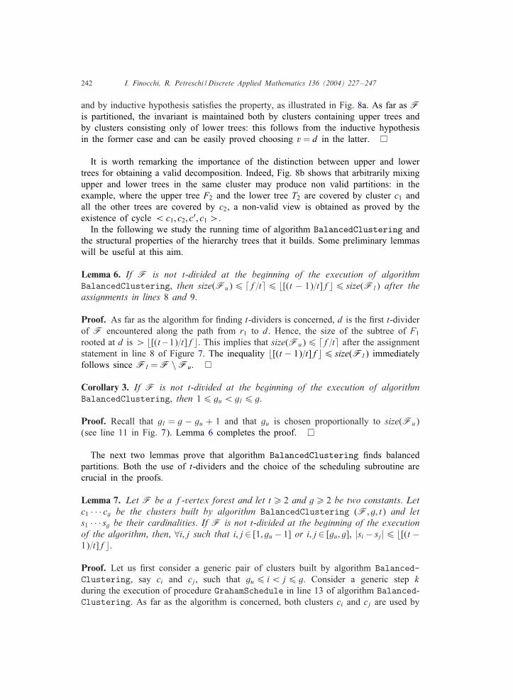
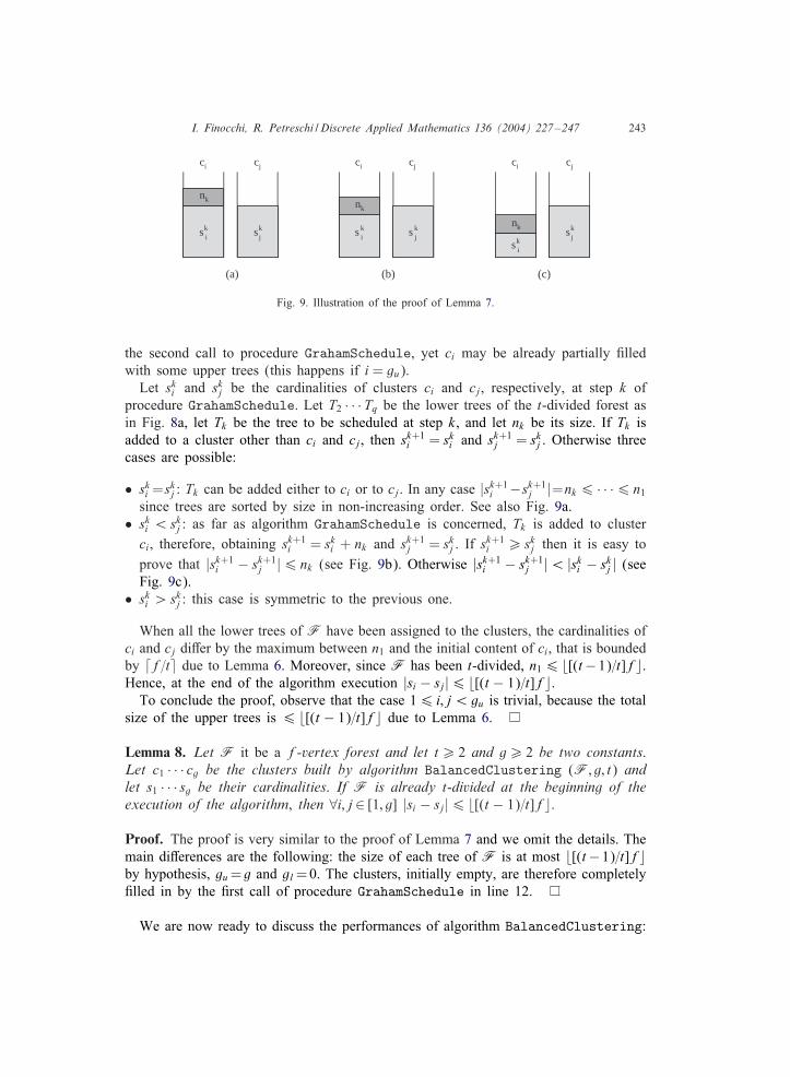
the second call to procedure GrahamSchedule, yet ci may be already partially @lledwith some upper trees (this happens if i = gu).Let sk

i and skj be the cardinalities of clusters ci and cj, respectively, at step k of

procedure GrahamSchedule. Let T2 · · ·Tq be the lower trees of the t-divided forest asin Fig. 8a, let Tk be the tree to be scheduled at step k, and let nk be its size. If Tk isadded to a cluster other than ci and cj, then sk+1

i = ski and sk+1

j = skj . Otherwise three

cases are possible:

• ski =sk

j : Tk can be added either to ci or to cj. In any case |sk+1i −sk+1

j |=nk 6 · · ·6 n1since trees are sorted by size in non-increasing order. See also Fig. 9a.

• ski ¡ sk

j : as far as algorithm GrahamSchedule is concerned, Tk is added to clusterci, therefore, obtaining sk+1

i = ski + nk and sk+1

j = skj . If sk+1

i ¿ skj then it is easy to

prove that |sk+1i − sk+1

j |6 nk (see Fig. 9b). Otherwise |sk+1i − sk+1

j |¡ |ski − sk

j | (seeFig. 9c).

• ski ¿ sk

j : this case is symmetric to the previous one.

When all the lower trees of F have been assigned to the clusters, the cardinalities ofci and cj di0er by the maximum between n1 and the initial content of ci, that is boundedby f=t� due to Lemma 6. Moreover, since F has been t-divided, n16 [(t−1)=t]f�.Hence, at the end of the algorithm execution |si − sj|6 [(t − 1)=t]f�.To conclude the proof, observe that the case 16 i; j ¡ gu is trivial, because the total

size of the upper trees is 6 [(t − 1)=t]f� due to Lemma 6.

Lemma 8. Let F it be a f-vertex forest and let t¿ 2 and g¿ 2 be two constants.Let c1 · · · cg be the clusters built by algorithm BalancedClustering (F; g; t) andlet s1 · · · sg be their cardinalities. If F is already t-divided at the beginning of theexecution of the algorithm, then ∀i; j ∈ [1; g] |si − sj|6 [(t − 1)=t]f�.

Proof. The proof is very similar to the proof of Lemma 7 and we omit the details. Themain di0erences are the following: the size of each tree of F is at most [(t−1)=t]f�by hypothesis, gu =g and gl =0. The clusters, initially empty, are therefore completely@lled in by the @rst call of procedure GrahamSchedule in line 12.

We are now ready to discuss the performances of algorithm BalancedClustering:


Theorem 3. Let T (V; E) be a n-vertex free tree and let g be the required maximumdegree of a hierarchy tree of T . Algorithm BalancedClustering computes a validhierarchy tree of T having depth O(log n) and degree 6 g in O(n log n) worst-caserunning time.

Proof. Let HT be the hierarchy tree grown by recursively applying algorithm Balanced-Clustering. Lemma 5 guarantees that HT is valid. As far as the algorithm works, itshould be also clear that the degree of HT is bounded by g. Let us now consider acluster c of HT and let nc be its cardinality. Let c1 · · · cg be the children of c in HT ,with cardinalities s1 · · · sg, respectively. Let m be the index of a maximum cardinalitychild of c. Our aim is to prove that sm is a constant fraction of nc: in particular, weshow that the speci@c constant depends on the value of t.We @rst consider the case where F = S(c) is not t-divided at the beginning of

the execution of algorithm BalancedClustering. The claim easily holds if m ¡ gu:Lemma 6 implies that the size of each cluster @lled in with only upper trees is at most f=t�. If m¿ gu, let r be an integer in [gu; g] such that r = m (such an index existsdue to Corollary 3). Due to Lemma 7:

sm − sr 6⌊

t − 1t

nc

⌋:

Moreover, since the algorithm partitions the vertices covered by c, the following equal-ity holds:

g∑i=1

si = nc:

Summing up the left and right sides of the above inequalities, respectively, it is easyto obtain

2sm +g∑

i=1i �=r;m

si6⌊2t − 1

tnc

⌋

and therefore sm6 [(2t−1)=2t]nc�. A very similar reasoning, with the help of Lemma8, holds if F is already t-divided at the beginning of the execution of the algorithm.Hence, since the cardinality of each cluster of the hierarchy tree is a constant fractionof the cardinality of its parent, the depth of HT is clearly O(log n).To conclude, we discuss the running time of algorithm BalancedClustering

(F; g; t). We denote by f and h the number of vertices and the number of trees offorest F, respectively. Since each tree is non-empty, h6f and lines 2 to 11 in Fig. 7can be easily implemented in O(f) time. If we assume that the children of each nodeof tree T are sorted by non-increasing size of the subtree of which they are the root,each call to procedure GrahamSchedule considers the trees in the given ordering and,for each tree, decides to which cluster it must be added by selecting the cluster cur-rently having the smallest cardinality (this choice can be done in O(1) time since g is aconstant). Hence, lines 12 and 13 in Fig. 7 can be implemented in O(f) time, as well.


In conclusion, during the recursive application of algorithm BalancedClustering tobuild the entire hierarchy tree, each vertex of tree T is visited in total as many timesas its depth in HT , thus giving total running time O(n log n).

The hierarchy tree shown in Fig. 6c is obtained running algorithm Balanced-Clustering on an 11-vertex star. The example shows that algorithm Balanced-Clustering is able to e0ectively balance the cardinalities of clusters. This goodresult is obtained in spite of loosing the property of connectivity. However, it is worthremarking that the disconnectivity of clusters remains “weak”, because for each pairof disconnected components in the same cluster there exist two representative verticeswhose distance on the original tree is equal to 2 (see Corollary 1 and the invariantproperty discussed in the proof of Lemma 5).

6. Concluding remarks

In this paper we have considered the problem of computing hierarchical decom-positions of trees. We have introduced the concept of t-divider, that generalizes thewell-known concepts of centroids and separators, and we have designed new tree parti-tioning algorithms hinging upon t-dividers. All the algorithms work by vertex deletionand aim at optimizing di0erent features of the hierarchy tree: among them, depth,maximum degree, and balancing deserve special attention.We have shown that bounded degree of the hierarchy tree is di3cult to achieve if

small depth and balanced cluster size have to be guaranteed: this is especially truewhen the maximum degree of the tree to be clustered is not constant and if discon-nected clusters are not allowed. We refer to Remarks 1–3 in Section 4 for a detaileddescription of the performances of the naQRve partitioning approaches. We have thenproved that all the above criteria can be optimized simultaneously if one is willing togive up internally connected clusters. This idea, together with a reduction to a classicalscheduling problem, allowed us to design a partitioning algorithm that, given a n-vertextree T , computes in O(n log n) time a balanced hierarchy tree of T having boundeddegree and logarithmic depth (see Lemmas 7 and 8, and Theorem 3 in Section 5 fordetails). We remark that P(n) is a trivial lower bound on the construction of anyhierarchy tree of T .All our algorithms also guarantee to build valid hierarchy trees, i.e., guarantee that

any contraction of the original tree on its hierarchy tree is itself a tree. This is es-pecially relevant in graph visualization applications, where hierarchical decompositionare commonly used. Building valid hierarchy trees may be di3cult when disconnectedclusters are allowed, and most of the partitioning algorithms from the literature that@nd disconnected clusters do not guarantee this property.In our opinion it would be interesting to extend this work towards two main direc-

tions. First, a generalization of the concepts and ideas presented throughout the paper tovertex- and edge-weighted trees would be a valuable improvement. This would make itpossible to apply the t-divider based algorithms to the block cut-vertex tree of a graph,assigning the weight of a tree vertex with the size of the corresponding biconnected


component. We remark that computing a partition of the block cut-vertex tree is auseful preliminary step in many graph decomposition algorithms.Furthermore, an extensive experimental study of tree decomposition algorithms could

be useful to point out bene@ts and disadvantages of partitioning strategies based eitheron vertex or on edge deletion. Some preliminary results along this line are reportedin [10], showing that the use of centroids, that is a common option for partitioningalgorithms based on vertex deletion, does not usually yield the best solution in practice.The best choice for t in most tests is t =3, i.e., partitioning using separators yields thebest hierarchy trees with respect to balancing, depth, and degree.

Acknowledgements

The authors wish to thank three anonymous referees for their careful review of thepaper and for their constructive comments.

References

[1] E. Agasi, R.I. Becker, Y. Perl, A shifting algorithm for constrained min–max partition of trees, DiscreteAppl. Math. 45 (1993) 1–28.

[2] R.I. Becker, Y. Perl, The shifting algorithm technique for the partitioning of trees, Discrete Appl. Math.62 (1995) 15–34.

[3] R.I. Becker, B. Simeone, Y.I. Chiang, How to make a polynomial movie from pseudopolynomiallymany frames: a continuous shifting algorithm for tree partitioning, Proceedings of Fun With Algorithms(FUN 98), Isola d’Elba, Italy, 1998, pp. 20–31.

[4] R.R. Benkoczi, B.K. Bhattacharya, Spine tree decomposition, Technical Report TR 1999-09, School ofComputing Science, Simon Fraser University, Burnaby, BC, Canada, 1999.

[5] A.L. Buchsbaum, J.R. Westbrook, Maintaining hierarchical graph views, Proceedings of the 11thACM-SIAM Symposium on Discrete Algorithms (SODA 00), San Francisco, USA, 2000, pp. 566–575.

[6] F. Buckley, F. Harary, Distance in Graphs, Addison Wesley, Reading, MA, 1990.[7] A.A. Diwan, S. Rane, S. Seshadri, S. Sudarshan, Clustering techniques for minimizing external path

length, Proceedings of the 22nd Very Large Databases Conference (VLDB 96), Mumbai (Bombay),India, 1996.

[8] I. Finocchi, Hierarchical decompositions for visualizing large graphs, Ph.D. Thesis, Department ofComputer Science, University of Rome “La Sapienza”, XIII-02-1, 2002.

[9] I. Finocchi, R. Petreschi, On the validity of hierarchical decompositions, Proceedings of the SeventhAnnual International Computing and Combinatorics Conference (COCOON 01), Lecture Notes inComputer Science, Guilin, China, Vol. 2108, 2001, pp. 368–374.

[10] I. Finocchi, R. Petreschi, Hierarchical clustering of trees: algorithms and experiments, Proceedings ofthe Third Workshop on Algorithm Engineering and Experimentation (ALENEX 01), Lecture Notes inComputer Science, Washington DC, USA, Vol. 2153, 2001, pp. 117–131.

[11] G.N. Frederickson, Data structures for on-line updating of minimum spanning trees, with applications,SIAM J. Comput. 14 (4) (1985) 781–798.

[12] M.R. Garey, D.S. Johnson, Computers and Intractability: A Guide to the Theory of NP-Completeness,W.H.Freeman, New York, 1979.

[13] R.L. Graham, Bounds for multiprocessing timing anomalies, SIAM J. Appl. Math. 17 (1969) 263–269.[14] S.E. Hambrusch, C. Liu, H. Lim, Clustering in trees: optimizing cluster sizes and number of subtrees,

J. Graph Algorithms Appl. 4 (4) (2000) 1–26.[15] D. Kuo, G.J. Chang, The pro@le minimization problem in trees, SIAM J. Comput. 23 (1) (1994)

71–81.


[16] R.J. Lipton, R.E. Tarjan, A separator theorem for planar graphs, SIAM J. Appl. Math. 36 (2) (1979)177–189.

[17] M. Lucertini, Y. Perl, B. Simeone, Most uniform path partitioning and its use in image processing,Discrete Appl. Math. 42 (1993) 227–256.

[18] T. Nishizeki, N. Chiba, Planar Graphs: Theory and Algorithms North Holland, Amsterdam, 1988.[19] Y. Perl, S. Schach, Max-min tree partitioning, J. ACM 28 (1981) 5–15.[20] Y. Perl, U. Vishkin, E3cient implementation of a shifting algorithm, Discrete Appl. Math. 12 (1985)

71–80.[21] R. Schrader, Approximations to clustering and subgraphs problems on trees, DAMATH: Discrete Appl.

Math. Combin. Oper. Res. Comput. Sci. 6 (1983) 301–309.

divider-based algorithms for hierarchical tree partitioning

Documents