BIS Papers No 58 49

Diversifying market and default risk in high grade sovereign bond portfolios

Myles Brennan, Adam Kobor1 and Vidhya Rustaman2

Introduction

Diversification is a keystone in modern finance. In this paper we discuss the potential benefits of diversification for high grade sovereign bond portfolios. A government bond investor may be motivated to diversify internationally for a number of reasons. The first and most classic reason would be to achieve overall volatility reduction in the portfolio. If the economic and business cycles of different countries are showing lags relative to each other, it is realistic to assume that lags across the expectations, monetary policy actions and other factors that influence interest rates would lead to less-than-perfect correlations. Beyond volatility reduction, investing in multiple countries could also be driven by return enhancement: the investor may find an attractive credit spread from a country with lower credit quality within the same currency zone, or the investor may expect positive carry from relative yield curve differences across different currencies. In conjunction, with an increasing focus on sovereign default risk, mitigating the impacts of possible financial distress may also be a motivation to diversify. In this paper we discuss both rate volatility reduction and the tail risk reduction aspects of diversification.

With globalization and free flow of capital, developed markets became highly integrated into the world market, and correlations across different countries have increased. The average correlation across the Bank of America/Merrill Lynch government indices of the G7 countries has been 0.66 over the past decade, but if we exclude Japan from the sample, in fact it would have been 0.78. These correlations suggest some diversification power, but clearly show a strong cross-border connection. We note that correlations across the MSCI equity indices of the G7 countries were similarly high over the past 10 years, on the order of 0.7. To get a more detailed and fundamental understanding of what drives government bond returns of a specific country, we apply a CAPM-based model to the G7 countries. This model attributes expected return to both global and local risk factors. If a market is fully integrated, its expected return depends solely on global risk factors and the market’s exposure to them. If markets were fully integrated, assets with the same risk should have equal expected returns. However, if a market is fully segmented, its expected return should be derived from local factors only. We find that G7 government bond markets are partially integrated to the global market, with an average of 75-80% of their expected excess return coming from global risk factors. However, the impact of local factors is still on the order of 20-25%, meaning that these markets are not fully integrated, and still there is some room for diversification.

While volatility reduction is a typical result of diversification, investors may be more concerned about mitigating the impact of tail risk due to financial distress. Recent developments in the Eurozone government bond markets serve to highlight this concern. The Eurozone shares a

1 Corresponding author; e-mail: akobor@worldbank.org. 2 Myles Brennan is Director; Adam Kobor is Principal Portfolio Manager; and Vidhya Rustaman is Senior

Portfolio Manager at the Investment Management Department of the World Bank Treasury.

The findings, interpretations and conclusions expressed herein are those of the authors and do not necessarily represent the views of the World Bank.

50 BIS Papers No 58

common monetary policy, so diversifying across issuers would have the impact of sharing exposure across different credit risk factors, and potentially picking up yields from lower credit quality borrowers. Recently, downside risk has been the dominant story for peripheral countries, driven by concerns about sovereign defaults, or the break-up of the Eurozone. Pure historical analysis is not sufficient for the assessment of diversification benefits against default losses, so we supplement our arguments with hypothetical simulation studies. Based on a default simulation exercise we find that diversification may mitigate severe credit losses, but the diversification may be limited due to the relatively low number of sovereign issuers.

This paper consists of two fairly distinct parts. The first part covers “business as usual” diversification, focusing on the reduction of volatility, and ignoring, or only implicitly considering, credit risk. This first part follows mainstream financial economic research, and historical time series can be used for reliable estimation. While in the second part we also apply historical estimations, we ultimately try to quantify the extremes, ie default loss. History in this context is less reliable, and the results are more dependent on qualitative assumptions and hypothetical scenarios. In 2010, we consider both aspects of diversification to be relevant.

The paper is organized as follows: first, we review the literature that deals with international government bond diversification and portfolio construction from both the academic and practitioner standpoint. In Section 2, we discuss diversification across G7 governments both in the context of asset pricing as well as from an empirical perspective. Then we turn our attention to sovereign credit risk considerations in Section 3. We review the recent history of risk and return within the Eurozone, applying a Markov switching model, and present credit risk simulation results based on hypothetical assumptions. Finally, we draw conclusions.

1. Literature review

Researchers discuss international diversification and global government bond portfolio construction from many different directions. International CAPM-based models discuss the degree to which national markets are integrated in the world market and explain the sources of risk and return. These models assume that the expected return comes from two systematic sources: the world market and the local market. Investing in a country that is fully integrated with the world market will only provide compensation against global market risk. In contrast, a fully segmented market will only provide compensation against local market risk. As fully integrated markets are likely to see the same expected returns for assets with the same risk, the case for diversification is more apparent if markets appear to be segmented. Several studies follow the paper by Bekaert and Harvey (1995), who tested the extent of integration in international equity markets. Barr and Priestley (2004) studied monthly returns in US, UK, German, Canadian and Japanese government markets between 1986 and 1996, and found that the average contribution of world factors to domestic returns was only 70%, implying that the full benefits of international diversification have not been realized in the international bond markets. In a more recent study discussing the integration of European government bond markets, Abad et al. (2009) found that based on a study of weekly returns over 1999 to 2008, euro-based countries are less sensitive to world risk factors, and are only partially integrated with the German market, suggesting room for diversification. Following an empirical statistical approach, Longstaff et al. (2008) find that excess return from sovereign credit is largely compensating for bearing global risk only, but find little country-specific credit risk premium after adjusting for global risk factors in general.

From the credit risk management perspective, the bulk of the literature discusses the risk of corporate bonds – see a broad review intended for risk practitioners by Ramaswamy (2004) among many others. Duffie and Singleton (2003) discuss credit risk from both the risk management and the asset pricing point of view, and they address both corporate as well as sovereign credit risk in their book. Wei (2003) discusses a multi-factor credit migration modeling approach that can be applied for both corporate and sovereign debts. Gray and

BIS Papers No 58 51

Malone (2008) extend Merton’s contingent claim approach to the macro level, including sovereign balance sheet analysis. Remolona et al. (2007) discuss the factors explaining sovereign credit spreads, and relate potential loss based on historical data provided by rating agencies to the size of the credit spread. They also raise the point that diversifying sovereign default risk is more limited than, say, risk diversification in equities due to the relatively low number of issuers. Reinhart and Rogoff’s (2009) book provides a historical synthesis of different kinds of crisis periods over several centuries, and we find it an essential read for understanding the nature of sovereign default risk.

Related to credit risk considerations, some practitioners suggest moving away from market weights as fixed income benchmarks given that these weights tend to overemphasize the more indebted countries. With respect to fixed income benchmarks, Laurence Siegel (2003) notes that market cap-weighted fixed income benchmarks bring rise to the “bums” problem, namely that the biggest debtors have the largest weights in the benchmarks and as a result, these benchmarks are unlikely to be mean-variance efficient. A number of practitioners have also increased focus on alternative weighting methodologies, including indices with weights linked to financial fundamental variables (Arnott et al. 2005 and Arnott el al. 2010), country weighting schemes related to GDP (see eg Barclays 2009 and PIMCO 2010), and indices with country level or regional caps (Dynkin and Ben Dor 2006).

2. Global diversification: searching for volatility reduction

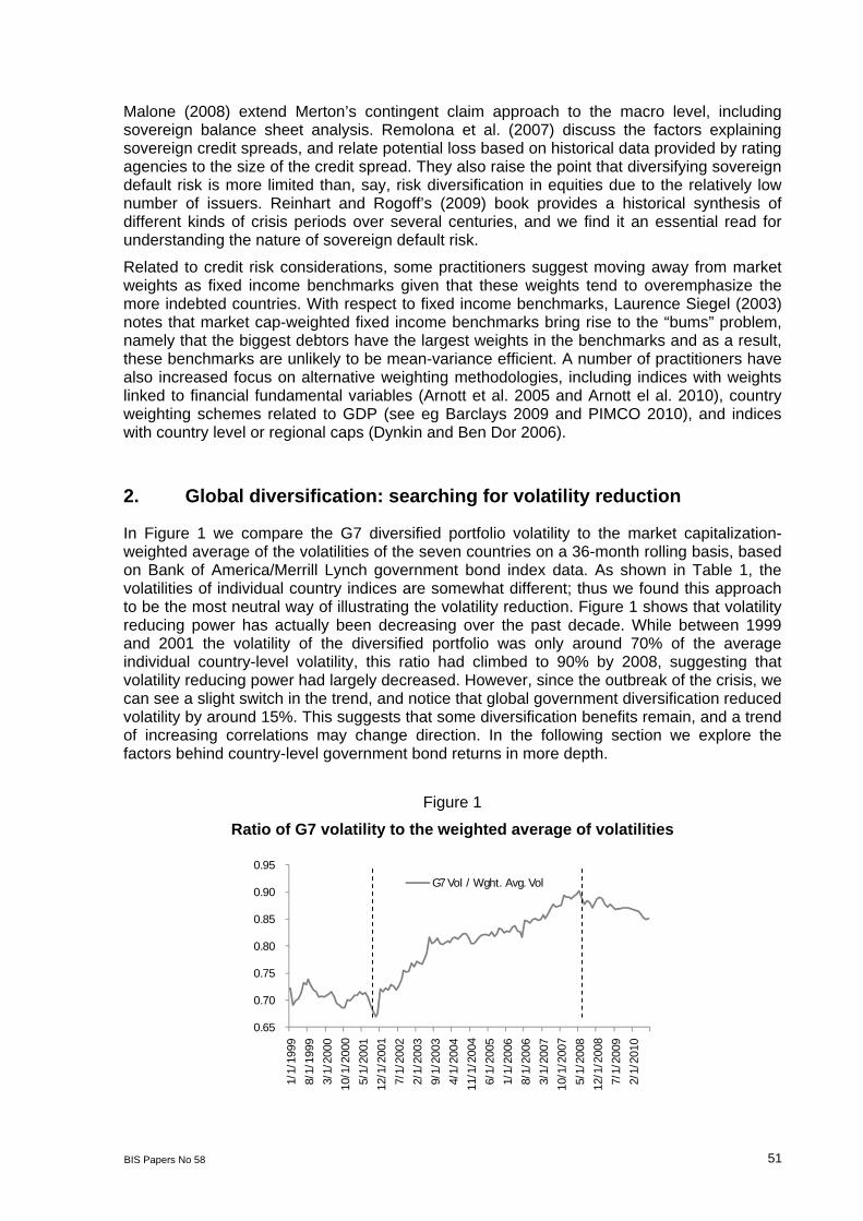
In Figure 1 we compare the G7 diversified portfolio volatility to the market capitalization-weighted average of the volatilities of the seven countries on a 36-month rolling basis, based on Bank of America/Merrill Lynch government bond index data. As shown in Table 1, the volatilities of individual country indices are somewhat different; thus we found this approach to be the most neutral way of illustrating the volatility reduction. Figure 1 shows that volatility reducing power has actually been decreasing over the past decade. While between 1999 and 2001 the volatility of the diversified portfolio was only around 70% of the average individual country-level volatility, this ratio had climbed to 90% by 2008, suggesting that volatility reducing power had largely decreased. However, since the outbreak of the crisis, we can see a slight switch in the trend, and notice that global government diversification reduced volatility by around 15%. This suggests that some diversification benefits remain, and a trend of increasing correlations may change direction. In the following section we explore the factors behind country-level government bond returns in more depth.

Figure 1

Ratio of G7 volatility to the weighted average of volatilities

0.65

0.70

0.75

0.80

0.85

0.90

0.95

1/1/

1999

8/1/

1999

3/1/

2000

10/1

/200

0

5/1/

2001

12/1

/200

1

7/1/

2002

2/1/

2003

9/1/

2003

4/1/

2004

11/1

/200

4

6/1/

2005

1/1/

2006

8/1/

2006

3/1/

2007

10/1

/200

7

5/1/

2008

12/1

/200

8

7/1/

2009

2/1/

2010

G7 Vol / Wght. Avg. Vol

52 BIS Papers No 58

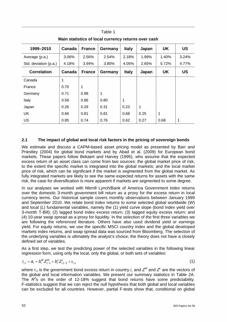
Table 1

Main statistics of local currency returns over cash

1999–2010 Canada France Germany Italy Japan UK US

Average (p.a.) 3.06% 2.56% 2.54% 2.18% 1.99% 1.40% 3.24%

Std. deviation (p.a.) 4.18% 3.94% 3.80% 4.05% 2.65% 5.72% 4.77%

Correlation Canada France Germany Italy Japan UK US

Canada 1

France 0.70 1

Germany 0.71 0.98 1

Italy 0.58 0.86 0.80 1

Japan 0.26 0.29 0.31 0.23 1

UK 0.66 0.81 0.81 0.68 0.25 1

US 0.85 0.74 0.76 0.62 0.27 0.68 1

2.1 The impact of global and local risk factors in the pricing of sovereign bonds

We estimate and discuss a CAPM-based asset pricing model as presented by Barr and Priestley (2004) for global bond markets and by Abad et al. (2009) for European bond markets. These papers follow Bekaert and Harvey (1995), who assume that the expected excess return of an asset class can come from two sources: the global market price of risk, to the extent the specific market is integrated into the global markets; and the local market price of risk, which can be significant if the market is segmented from the global market. As fully integrated markets are likely to see the same expected returns for assets with the same risk, the case for diversification is more apparent if markets are segmented to some degree.

In our analyses we worked with Merrill Lynch/Bank of America Government index returns over the domestic 3-month government bill return as a proxy for the excess return in local currency terms. Our historical sample covers monthly observations between January 1999 and September 2010. We relate bond index returns to some selected global worldwide (W) and local (L) fundamental variables, namely the (1) yield curve slope (bond index yield over 3-month T-Bill); (2) lagged bond index excess return; (3) lagged equity excess return; and (4) 10-year swap spread as a proxy for liquidity. In the selection of the first three variables we are following the referenced literature. Others have also used dividend yield or earnings yield. For equity returns, we use the specific MSCI country index and the global developed markets index returns, and swap spread data was sourced from Bloomberg. The selection of the underlying variables is ultimately the analyst’s choice; the theory does not have a closely defined set of variables.

As a first step, we test the predicting power of the selected variables in the following linear regression form, using only the local, only the global, or both sets of variables:

, 1 , 1 ,W W L L

i t i i t i i t i tr a b Z b Z (1)

where ri,t is the government bond excess return in country i¸ and ZW and ZL are the vectors of the global and local information variables. We present our summary statistics in Table 2A. The R2s on the order of 12-18% suggest that bond returns have some predictability. F-statistics suggest that we can reject the null hypothesis that both global and local variables can be excluded for all countries. However, partial F-tests show that, conditional on global

BIS Papers No 58 53

variables, except for Japan, the omission of local variables cannot be rejected. Similarly, conditional on local variables, the omission of global variables cannot be rejected in the cases of Canada, Italy, and the US. We also present R2s and F-statistics for regressions based on local and global variables only; based on these, except for global variables in Japan, we cannot reject the null hypothesis of the omission of the selected factors. We have to mention that the selected global and local information variables are correlated – see the correlations between the local bond returns, and also our observation on equities in the introduction. Thus, it may be understandable that the local-only or global-only regressions show significance, but we cannot reject the null hypothesis of omitting one set of the variables in several cases of the joint regressions. These correlations across global and local variables may impose some limitations on the analyses, but we still prefer using market-based variables as they should immediately reflect market perception, and unlike some macroeconomic variables they are not subject to reporting time lags, or revisions and methodological differences across countries. Nevertheless, had we chosen to work with, say, inflation and industrial production variables, they would also be correlated.

The actual conditional international CAPM takes the following form:

cov , 1 var, , 1 1 , , , 1 1 , ,r r r ri t i W t t W t i t i i t t i t i t (2)

The first component of the equation represents the compensation for the global market risk:

, 1W t is the time-varying global market price of risk; 1 , ,cov ,t W t i tr r is the covariance of

market i with the global bond market and measures the sensitivity to the global market price of risk, and i is the degree of integration into the global market. The second part of the

formula represents the compensation for local risk, and , 1i t is the local price of risk. The

dynamics of the global bond market are given by:

, , 1 1 , ,varW t W t t W t W tr r (3)

and the error terms from equations (2) and (3) are assumed to be normally distributed with

GARCH (1,1) covariances, ie [ ] ~ 0,, , N Ht i t W t t with:

1 11

t tt tH C C A A B H B

(4)

The main significance of working with GARCH variances and covariances is that they allow for time-varying risk exposure in our model. In addition, the time-varying market price of risk is assumed to take non-negative values; thus, similarly to the literature, we express market price of risk in the form of exponential functions:

', 1 1exp w

w t w tK (5)

', 1 , 1exp L

i t i i t (6)

We estimate the parameters by maximum-likelihood method in two steps. First, we estimate the parameters of equation (3). Then, in step two we estimate equation (2) for each country, using the world market price of risk as input obtained in step one, and we fix the univariate GARCH parameter estimates a22 and b22 for the global world market to ensure consistency. For the sake of numerical tractability, we also assume A and B to be diagonal. The parameter estimates are found in the second panel of Table 2. Based on their i estimates, Canada and the US appear to be the most integrated countries, whereas local factors and segmentation matter the most in Japan. European countries, except Italy, also show a relatively high degree of integration. We note that the asset pricing estimates and previous linear regression results seem to show similar messages. In the case of Japan, the global variables-only regression suggested that global variables may be less relevant, and the joint

54 BIS Papers No 58

regression kept local variables significant conditionally on global variables. In the asset pricing context, Japan is estimated to be the least integrated country over our sample time period.

In terms of the local risk premium, yield curve slope seems to consistently play a significant role based on our estimations, whereas there is more variation in the significance of lagged bond and equity returns as well as in the role of swap spreads.

Our i estimates are comparable to those reported by Barr and Priestley (2004). In our case, the average degree of integration is 0.8 and 0.75 on an equally weighted and market weighted basis, respectively. Barr and Priestley report an average of 0.7 for the five countries that they analyzed. The sample period in their case, however, was 1986 to 1996, so it is intuitive to see higher values in the case of a more recent period. Abad et al (2009) report lower estimated figures, but they worked with weekly observations. We similarly found lower figures in our experiments on a weekly basis; however, we consider the monthly horizon to be more relevant in the assessment of diversification benefits for institutional investors.

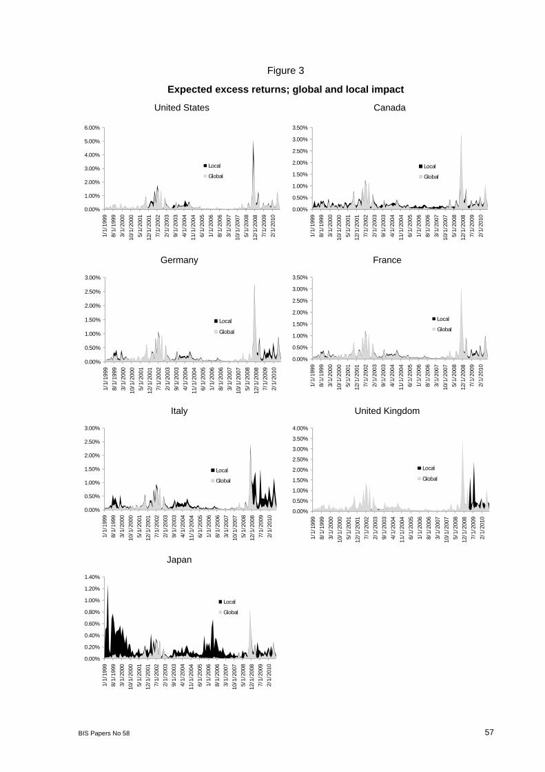
In Figure 2 we show the expected excess returns for the global bond market. The global premium took its highest levels at the most stressful periods of the crisis. In Figure 3 we present expected returns for all the seven countries, and we separately show the global and local return components.

Figure 2

World bond market expected excess return

0.00%

0.50%

1.00%

1.50%

2.00%

2.50%

3.00%

3.50%

1/1/

1999

8/1/

1999

3/1/

2000

10/1

/200

0

5/1/

2001

12/1

/200

1

7/1/

2002

2/1/

2003

9/1/

2003

4/1/

2004

11/1

/200

4

6/1/

2005

1/1/

2006

8/1/

2006

3/1/

2007

10/1

/200

7

5/1/

2008

12/1

/200

8

7/1/

2009

2/1/

2010

Projected Excess Return W

Figure 3 provides insights into the dynamics of country-level expected returns, and shows the breakdown of excess returns by country. While the degree of integration is assumed to be constant over the period, the charts highlight the time-varying contribution by local factors due to time-varying risk premium and time-varying sensitivities:

The US has been a very highly integrated country, and only seemed to provide extra local premium on top of the global premium when the global premium was already high. Such periods include the tech bubble burst period around 2002 and the collapse of Lehman Brothers in 2008. US Treasuries did not seem to diversify against global governments, but rather intensified compensation in turbulent times. This is understandable if we consider US Treasuries the safe haven in a global flight to quality period;

Canada, while estimated to be very highly integrated, seemed to provide a smoother and more balanced compensation over time;

BIS Papers No 58 55

Germany and France are largely integrated, although they seemed to add some Eurozone-specific compensation over the past two years;

Italy is integrated to a lesser degree than Germany and France, and the local risk premium picked up in Italy over the past two years, since sovereign credit became a concern;

The UK is largely integrated, but also showed extra compensation recently, in line with signs of weakness in its banking system;

Finally, Japan is estimated to be the least integrated out of the seven countries. The data shows that the local premium in the earlier years seemed to be more important than recently.

The results presented in Figure 3 and Table 1 suggest that Japan was a main contributor to diversification in the G7 over the past decade. Japan had the lowest volatility, as well as the lowest pairwise correlations with the other countries over the past decade. With a weight around 35% in the G7 universe, Japan was clearly the main diversifier for non-yen investors (see market weights in Appendix 1.) However, in Figure 4 we can see that the local return component played a more important role during the earlier years of historical sample. At the same time, the local component seemed to have gained importance for European countries over the past two years or so, and this coincides with the recently improving volatility reduction trend highlighted in Figure 1.

The practical conclusion of this analysis is that sovereign government bonds are relatively highly integrated into the global market, but local factors still play a role. In the asset pricing context this means that the expected return is not solely dependent on global factors. Bonds with the same global risk factor sensitivities may offer somewhat different expected returns even if their global risk sensitivity is the same. Given that local factors are not negligible, the case for diversification still holds.

56

BIS

Papers N

o 58

Table 2

Asset pricing model estimation A. Predicting equations (OLS)

World Canada France Germany Italy Japan UK US

R2 (%) - 14.88 18.17 16.07 15.39 12.47 16.29 12.33

F-stat exclude local - 1.79 1.76 1.18 1.50 2.77* 1.64 0.77

F-stat exclude global - 0.42 2.64* 2.03* 1.92 2.19* 2.14* 0.53

Global and local variables

F-stat exclude both - 2.84* 3.61* 3.11* 2.96* 2.32* 3.16* 2.29*

R2 (%) - 13.77 11.52 11.45 10.40 6.56 10.77 10.91 Local variables only F-stat exclude local - 5.35* 4.36* 4.33* 3.89* 2.35* 4.05* 4.10*

R2 (%) 13.97 10.20 13.73 13.03 11.50 5.01 11.95 10.26 Global variables only F-stat exclude global 5.44* 3.80* 5.33* 5.02* 4.35* 1.77 4.55* 3.83*

*significant at least at 90% confidence level

B. Asset pricing model parameters (ML)

κ0 κ1 κ2 κ3 κ4 c a b

World 1.29* 128.04* 44.66 -16.18* -40.94* 0.0000* 0.0050* 0.7721*

θi δ0 δ1 δ2 δ3 δ4 c11 c12 c22 a11 b11

Canada 0.96* 4.84* 0.61 -55.91* -2.85 -2.57 0.0017* 0.0022* 0.0029* 0.0193* 0.8780*

France 0.86* 1.58* 100.91* 19.19* -2.57 -5.91 0.0026* 0.0026* 0.0026* 0.2255* 0.9033*

Germany 0.78* 0.06 202.62* 8.89 -5.88 -28.31* 0.0031* 0.0032* 0.0019* 0.2388* 0.8780*

Italy 0.63* -0.51 196.38* 30.84* -5.27 0.51 0.0041* 0.0035* 0.0010* 0.2347* 0.7746*

Japan 0.58* 0.27 409.50* 14.62 11.43 -543.12* 0.0000* 0.0031* 0.0019* 0.0000* 0.8830*

UK 0.88* -1.51* 142.48* -19.02* 40.32* -5.91 0.0036* 0.0035* 0.0012* 0.2597* 0.8907*

US 0.92* -0.51 193.21* -30.88* -16.35* -4.32 0.0032* 0.0032* 0.0017* 0.1797* 0.9165*

*significant at least at 90% confidence level.

κ and δ coefficients belong to the following factors: (1) yield curve slope; (2) lagged fixed income return; (3) lagged equity return; (4) swap spread.

BIS Papers No 58 57

Figure 3

Expected excess returns; global and local impact

United States Canada

0.00%

1.00%

2.00%

3.00%

4.00%

5.00%

6.00%

1/1/

1999

8/1/

1999

3/1/

2000

10/1

/200

0

5/1/

2001

12/1

/200

1

7/1/

2002

2/1/

2003

9/1/

2003

4/1/

2004

11/1

/200

4

6/1/

2005

1/1/

2006

8/1/

2006

3/1/

2007

10/1

/200

7

5/1/

2008

12/1

/200

8

7/1/

2009

2/1/

2010

Local

Global

0.00%

0.50%

1.00%

1.50%

2.00%

2.50%

3.00%

3.50%

1/1/

1999

8/1/

1999

3/1/

2000

10/1

/200

0

5/1/

2001

12/1

/200

1

7/1/

2002

2/1/

2003

9/1/

2003

4/1/

2004

11/1

/200

4

6/1/

2005

1/1/

2006

8/1/

2006

3/1/

2007

10/1

/200

7

5/1/

2008

12/1

/200

8

7/1/

2009

2/1/

2010

Local

Global

Germany France

0.00%

0.50%

1.00%

1.50%

2.00%

2.50%

3.00%

1/1/

1999

8/1/

1999

3/1/

2000

10/1

/200

0

5/1/

2001

12/1

/200

1

7/1/

2002

2/1/

2003

9/1/

2003

4/1/

2004

11/1

/200

4

6/1/

2005

1/1/

2006

8/1/

2006

3/1/

2007

10/1

/200

7

5/1/

2008

12/1

/200

8

7/1/

2009

2/1/

2010

Local

Global

0.00%

0.50%

1.00%

1.50%

2.00%

2.50%

3.00%

3.50%

1/1/

1999

8/1/

1999

3/1/

2000

10/1

/200

0

5/1/

2001

12/1

/200

1

7/1/

2002

2/1/

2003

9/1/

2003

4/1/

2004

11/1

/200

4

6/1/

2005

1/1/

2006

8/1/

2006

3/1/

2007

10/1

/200

7

5/1/

2008

12/1

/200

8

7/1/

2009

2/1/

2010

Local

Global

Italy United Kingdom

0.00%

0.50%

1.00%

1.50%

2.00%

2.50%

3.00%

1/1/

1999

8/1/

1999

3/1/

2000

10/1

/200

0

5/1/

2001

12/1

/200

1

7/1/

2002

2/1/

2003

9/1/

2003

4/1/

2004

11/1

/200

4

6/1/

2005

1/1/

2006

8/1/

2006

3/1/

2007

10/1

/200

7

5/1/

2008

12/1

/200

8

7/1/

2009

2/1/

2010

Local

Global

0.00%

0.50%

1.00%

1.50%

2.00%

2.50%

3.00%

3.50%

4.00%

1/1/

1999

8/1/

1999

3/1/

2000

10/1

/200

0

5/1/

2001

12/1

/200

1

7/1/

2002

2/1/

2003

9/1/

2003

4/1/

2004

11/1

/200

4

6/1/

2005

1/1/

2006

8/1/

2006

3/1/

2007

10/1

/200

7

5/1/

2008

12/1

/200

8

7/1/

2009

2/1/

2010

Local

Global

Japan

0.00%

0.20%

0.40%

0.60%

0.80%

1.00%

1.20%

1.40%

1/1/

1999

8/1/

1999

3/1/

2000

10/1

/200

0

5/1/

2001

12/1

/200

1

7/1/

2002

2/1/

2003

9/1/

2003

4/1/

2004

11/1

/200

4

6/1/

2005

1/1/

2006

8/1/

2006

3/1/

2007

10/1

/200

7

5/1/

2008

12/1

/200

8

7/1/

2009

2/1/

2010

Local

Global

58 BIS Papers No 58

2.2 An empirical look at the G7 portfolio

We complete our analysis by taking another empirical look at the G7 index volatility and performance. Table 3 summarizes a standard PCA analysis. We find that 76.4% of the variation in local currency excess returns of the seven markets can be explained by one factor. This first factor can be interpreted as the global bond market return, whereas the second factor appears to be a North America versus continental Europe factor, the third factor is UK-specific, and the fourth factor is a Japan-specific factor. Interestingly, we obtained a similar order of magnitude for global risk with PCA analysis as we did in the asset pricing analysis.

Table 3

Principal Component Analysis: variance explained and factor coefficients

Factor F1 F2 F3 F4

%ge explained 76.4% 7.4% 6.5% 5.5%

Canada 0.38 0.44 0.22 -0.06

France 0.37 -0.44 0.05 -0.06

Germany 0.36 -0.37 0.05 -0.03

Italy 0.30 -0.53 0.12 -0.16

Japan 0.09 -0.04 0.45 0.88

UK 0.51 0.18 -0.76 0.32

US 0.48 0.41 0.39 -0.30

Following the base currency neutral view of the G7 universe, illustratively we compare the G7 portfolio to a specific single currency alternative, namely US Treasuries. As Figure 4 shows, the volatility of the US Treasuries index was around 4.9% between January 2000 and August 2010, whereas the market cap weighted G7 index had a volatility of 3.0% after being hedged back to USD. In addition, the average return was not much behind: US Treasuries earned 6.5%, whereas the hedged index made 5.8%, thus showing a higher Sharpe ratio of 1.1 versus the UST-only alternative’s Sharpe ratio of 0.8, using 3-month T-Bills as the risk-free asset.

Figure 4

Historical risk-return space from a USD-based investor’s point of view

2000–2010

US Govt

German GovtH$

Japan Govt H$

G-7 H$

G-7 ex-Japan H$

5.0%

5.2%

5.4%

5.6%

5.8%

6.0%

6.2%

6.4%

6.6%

2.0% 2.5% 3.0% 3.5% 4.0% 4.5% 5.0% 5.5%

Ave

rage

retu

rn

Volatility

BIS Papers No 58 59

As previously shown in Table 1, US Treasuries had one of the highest excess return volatilities measured in local currency terms. Excess return volatility differences across the countries can be explained mainly by different levels of rate volatilities, but the durations of certain country indices were also somewhat different. We did not adjust durations to be equal in this paper, but even if we had, we would arrive at similar conclusions. That being said, given that US Treasuries exhibited the second highest volatility out of the seven countries, a dollar-based investor would have experienced a significant volatility reduction by simply switching from a US Treasuries-only portfolio to a G7 portfolio. The reduction in volatility as a result of a similar switch would seem to be smaller for a euro-based investor, and a yen-based investor would actually experience higher volatility. However, a G7 portfolio can still play an attractive role even for these investors in a portfolio optimization context.

Besides the differences in bond returns measured in local currency terms, currency hedging also has an impact on the ultimate performance of the diversified portfolio. Winkelmann (2003) finds that currency hedging is essential for bond portfolios as currency volatility exceeds government bond return volatility. Actually, applying our analysis to excess returns is consistent with analyzing hedged returns: the hedged return of a global bond portfolio is actually the same as the individual excess returns over cash, plus the cash return of the base currency. This is evident from covered interest rate parity. Figure 5 compares the bond index returns in local currency terms as well as in USD terms on a hedged basis between 1999 and 2010. Japanese cash rates were much lower than in the US during most of the period; thus, investing in Japanese bonds was very attractive on a currency hedged basis. We can consider this aspect similar to a typical carry trade. This also explains why the average return of the G7 hedged index did not fall much behind the US Treasury bond portfolio. Although this carry consideration goes beyond the scope of our paper, we note that the carry advantage from the perspective of a dollar-based investor has been diminished as cash rates are on a very similar scale at the moment of writing this paper. Ultimately, the optimization results for currency hedged bond portfolios depend on the expected excess returns, the excess return volatilities, and the correlations across the selected bond markets.

Figure 5

The impact of currency hedging

0.00%

1.00%

2.00%

3.00%

4.00%

5.00%

6.00%

7.00%

Canada France Germany Italy Japan UK US

Average LCY

Average $H

60 BIS Papers No 58

3. International diversification in the presence of credit risk

3.1 Switch in the Eurozone landscape

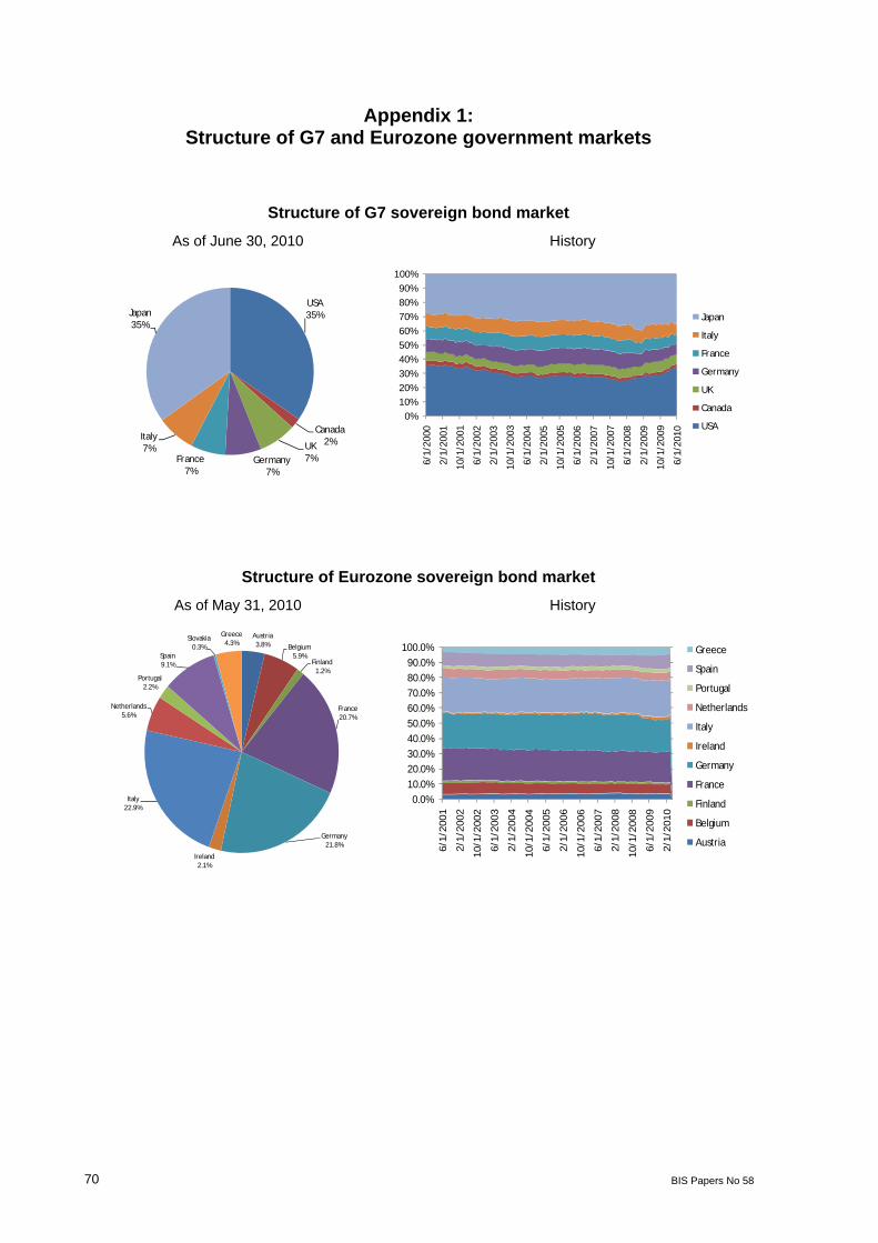
While behavior in G7 bond markets overall was relatively stable over the past decade, the markets in the periphery of the Eurozone became turbulent, as market participants became concerned at the path of increasing indebtedness in a number of Eurozone economies. For our analysis, we examine 11 Eurozone government bond markets, but we exclude Cyprus, Luxembourg, Malta, Slovakia and Slovenia due to their shorter histories within the Eurozone, or because of the lack of bond index data. We use bond index data from Bank of America/Merrill Lynch and Barclays Capital, and we cover the monthly history of index returns between July 31, 2001 and June 2010. Appendix 1 shows the latest market cap shares of the 11 countries in the Eurozone proxy, as well as the historical dynamics of the relative weights. We note that Barclays Capital stopped reporting index data for Greece after May 31, 2010, as Greece lost its eligibility as an investment grade country because of its S&P rating.

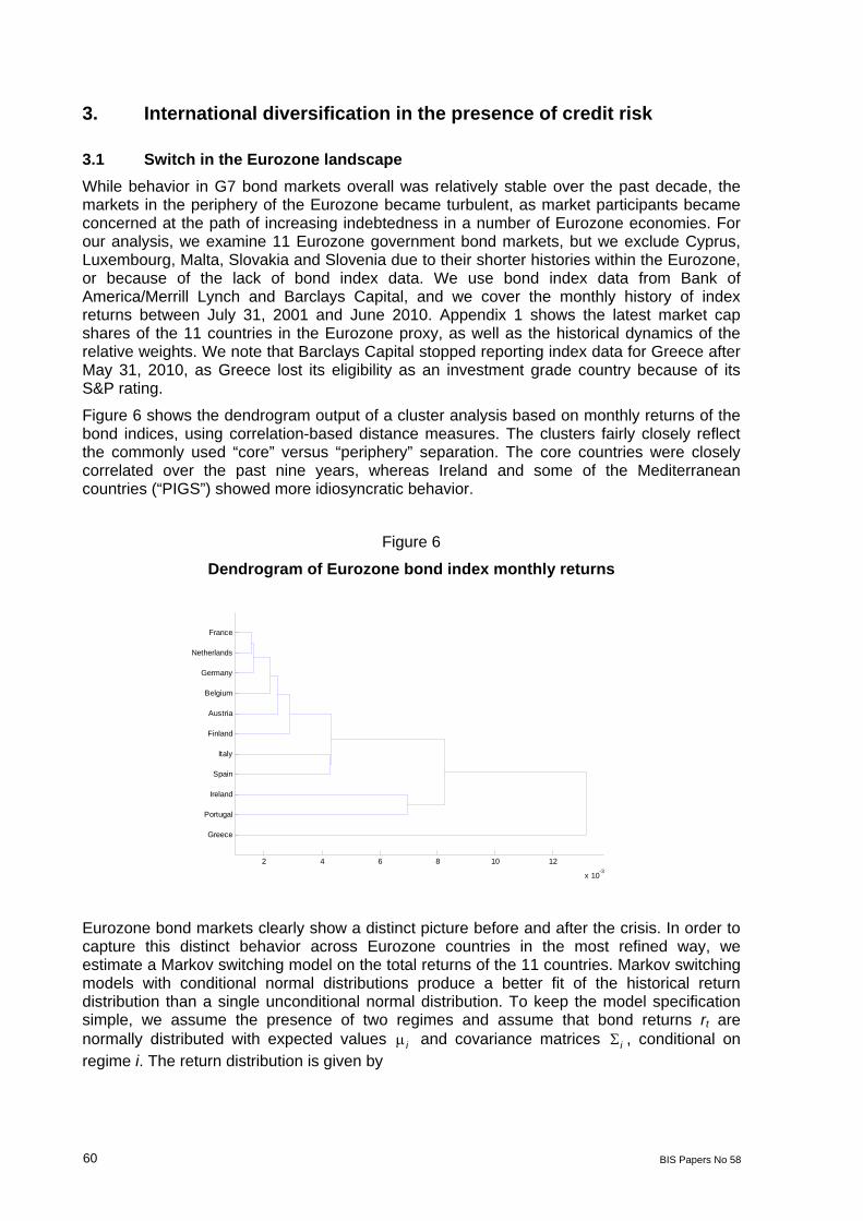
Figure 6 shows the dendrogram output of a cluster analysis based on monthly returns of the bond indices, using correlation-based distance measures. The clusters fairly closely reflect the commonly used “core” versus “periphery” separation. The core countries were closely correlated over the past nine years, whereas Ireland and some of the Mediterranean countries (“PIGS”) showed more idiosyncratic behavior.

Figure 6

Dendrogram of Eurozone bond index monthly returns

France

Netherlands

Germany

Belgium

Austria

Finland

Italy

Spain

Ireland

Portugal

Greece

2 4 6 8 10 12

x 10-3

Eurozone bond markets clearly show a distinct picture before and after the crisis. In order to capture this distinct behavior across Eurozone countries in the most refined way, we estimate a Markov switching model on the total returns of the 11 countries. Markov switching models with conditional normal distributions produce a better fit of the historical return distribution than a single unconditional normal distribution. To keep the model specification simple, we assume the presence of two regimes and assume that bond returns rt are normally distributed with expected values i and covariance matrices i , conditional on regime i. The return distribution is given by

BIS Papers No 58 61

' 1

12 2

1 1exp

22 detit t t i t iim

i

r s i y y

, (7)

where st denotes the regime or state in period t. The regimes are assumed to evolve as a Markov chain: the probability of regime st=j (j=1...N) only depends on the previous observation:

1 2 1, ,...t t t t ijt j s i s kP s P s j s i P

, (8)

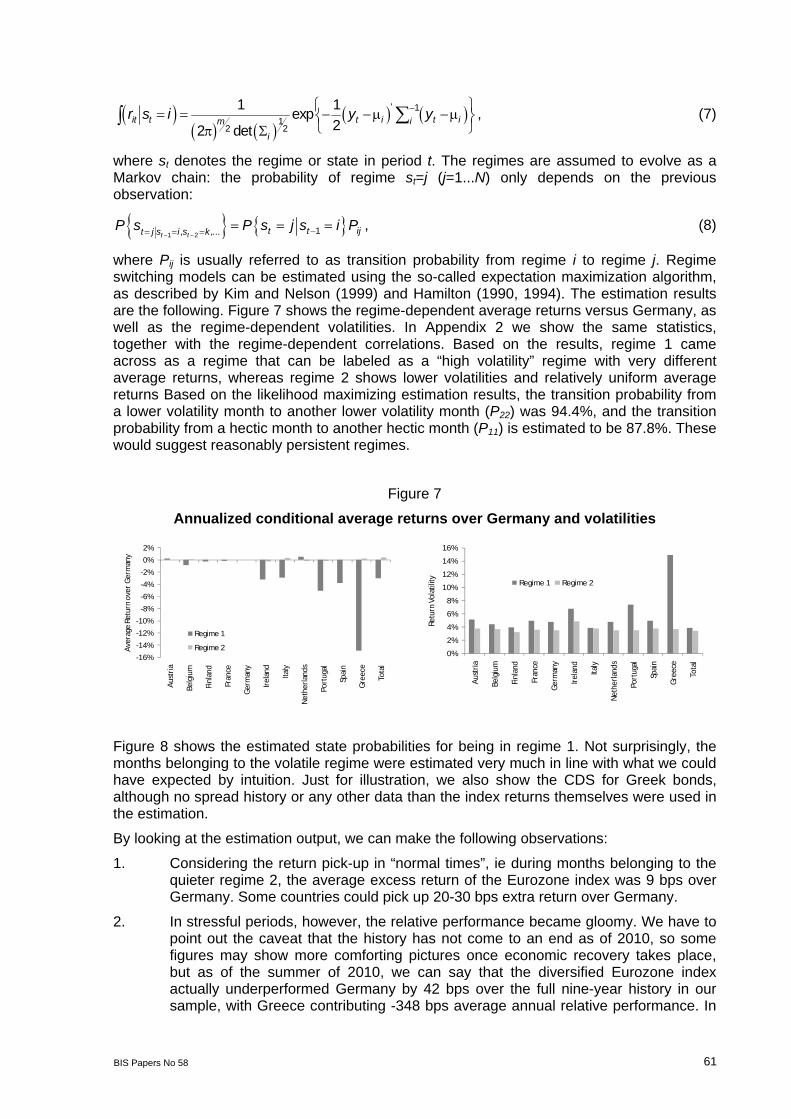
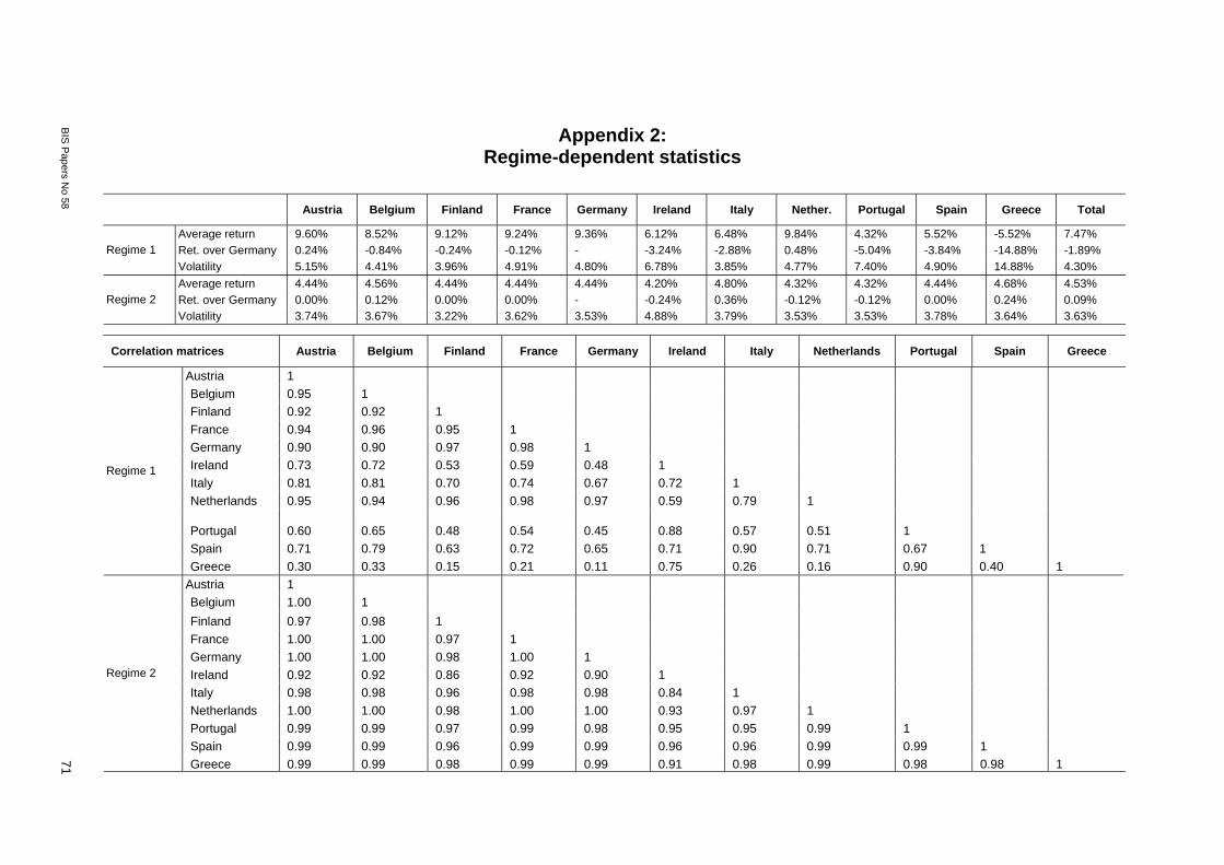
where Pij is usually referred to as transition probability from regime i to regime j. Regime switching models can be estimated using the so-called expectation maximization algorithm, as described by Kim and Nelson (1999) and Hamilton (1990, 1994). The estimation results are the following. Figure 7 shows the regime-dependent average returns versus Germany, as well as the regime-dependent volatilities. In Appendix 2 we show the same statistics, together with the regime-dependent correlations. Based on the results, regime 1 came across as a regime that can be labeled as a “high volatility” regime with very different average returns, whereas regime 2 shows lower volatilities and relatively uniform average returns Based on the likelihood maximizing estimation results, the transition probability from a lower volatility month to another lower volatility month (P22) was 94.4%, and the transition probability from a hectic month to another hectic month (P11) is estimated to be 87.8%. These would suggest reasonably persistent regimes.

Figure 7

Annualized conditional average returns over Germany and volatilities

-16%

-14%

-12%

-10%

-8%

-6%

-4%

-2%

0%

2%

Aus

tria

Belg

ium

Finl

and

Fran

ce

Ger

man

y

Irel

and

Italy

Net

herl

ands

Port

ugal

Spai

n

Gre

ece

Tota

l

Ave

rage

Ret

urn

over

Ger

man

y

Regime 1

Regime 20%

2%

4%

6%

8%

10%

12%

14%

16%

Aus

tria

Belg

ium

Finl

and

Fran

ce

Ger

man

y

Irel

and

Italy

Net

herl

ands

Port

ugal

Spai

n

Gre

ece

Tota

l

Retu

rn V

olat

ility Regime 1 Regime 2

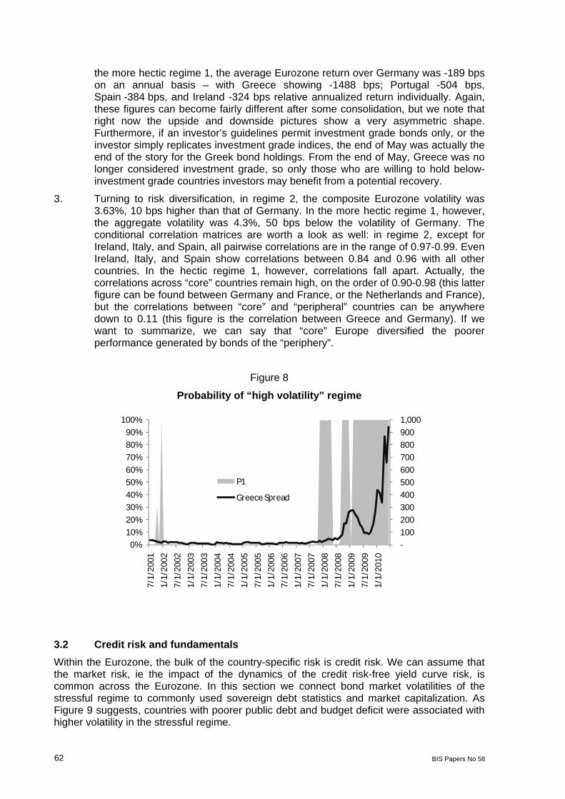
Figure 8 shows the estimated state probabilities for being in regime 1. Not surprisingly, the months belonging to the volatile regime were estimated very much in line with what we could have expected by intuition. Just for illustration, we also show the CDS for Greek bonds, although no spread history or any other data than the index returns themselves were used in the estimation.

By looking at the estimation output, we can make the following observations:

1. Considering the return pick-up in “normal times”, ie during months belonging to the quieter regime 2, the average excess return of the Eurozone index was 9 bps over Germany. Some countries could pick up 20-30 bps extra return over Germany.

2. In stressful periods, however, the relative performance became gloomy. We have to point out the caveat that the history has not come to an end as of 2010, so some figures may show more comforting pictures once economic recovery takes place, but as of the summer of 2010, we can say that the diversified Eurozone index actually underperformed Germany by 42 bps over the full nine-year history in our sample, with Greece contributing -348 bps average annual relative performance. In

62 BIS Papers No 58

the more hectic regime 1, the average Eurozone return over Germany was -189 bps on an annual basis – with Greece showing -1488 bps; Portugal -504 bps, Spain -384 bps, and Ireland -324 bps relative annualized return individually. Again, these figures can become fairly different after some consolidation, but we note that right now the upside and downside pictures show a very asymmetric shape. Furthermore, if an investor’s guidelines permit investment grade bonds only, or the investor simply replicates investment grade indices, the end of May was actually the end of the story for the Greek bond holdings. From the end of May, Greece was no longer considered investment grade, so only those who are willing to hold below-investment grade countries investors may benefit from a potential recovery.

3. Turning to risk diversification, in regime 2, the composite Eurozone volatility was 3.63%, 10 bps higher than that of Germany. In the more hectic regime 1, however, the aggregate volatility was 4.3%, 50 bps below the volatility of Germany. The conditional correlation matrices are worth a look as well: in regime 2, except for Ireland, Italy, and Spain, all pairwise correlations are in the range of 0.97-0.99. Even Ireland, Italy, and Spain show correlations between 0.84 and 0.96 with all other countries. In the hectic regime 1, however, correlations fall apart. Actually, the correlations across “core” countries remain high, on the order of 0.90-0.98 (this latter figure can be found between Germany and France, or the Netherlands and France), but the correlations between “core” and “peripheral” countries can be anywhere down to 0.11 (this figure is the correlation between Greece and Germany). If we want to summarize, we can say that “core” Europe diversified the poorer performance generated by bonds of the “periphery”.

Figure 8

Probability of “high volatility” regime

-

100

200

300

400

500

600

700

800

900

1,000

0%

10%

20%

30%

40%

50%

60%

70%

80%

90%

100%

7/1/

2001

1/1/

2002

7/1/

2002

1/1/

2003

7/1/

2003

1/1/

2004

7/1/

2004

1/1/

2005

7/1/

2005

1/1/

2006

7/1/

2006

1/1/

2007

7/1/

2007

1/1/

2008

7/1/

2008

1/1/

2009

7/1/

2009

1/1/

2010

P1

Greece Spread

3.2 Credit risk and fundamentals

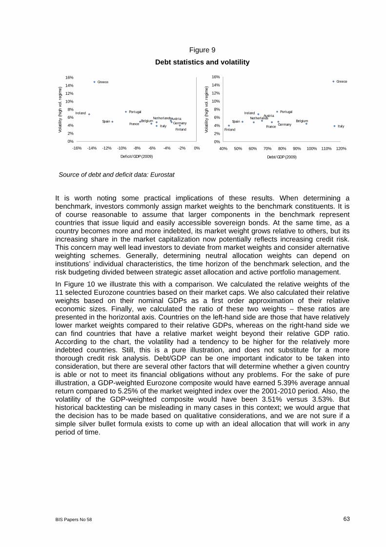
Within the Eurozone, the bulk of the country-specific risk is credit risk. We can assume that the market risk, ie the impact of the dynamics of the credit risk-free yield curve risk, is common across the Eurozone. In this section we connect bond market volatilities of the stressful regime to commonly used sovereign debt statistics and market capitalization. As Figure 9 suggests, countries with poorer public debt and budget deficit were associated with higher volatility in the stressful regime.

BIS Papers No 58 63

Figure 9

Debt statistics and volatility

AustriaBelgium

Finland

France Germany

Ireland

Italy

Netherlands

Portugal

Spain

Greece

0%

2%

4%

6%

8%

10%

12%

14%

16%

-16% -14% -12% -10% -8% -6% -4% -2% 0%

Vola

tility

(hi

gh v

ol. r

egim

e)

Deficit/GDP (2009)

Austria

Belgium

FinlandFrance

Germany

Ireland

Italy

Netherlands

Portugal

Spain

Greece

0%

2%

4%

6%

8%

10%

12%

14%

16%

40% 50% 60% 70% 80% 90% 100% 110% 120%

Vola

tility

(hi

gh v

ol. r

egim

e)

Debt/GDP (2009)

Source of debt and deficit data: Eurostat

It is worth noting some practical implications of these results. When determining a benchmark, investors commonly assign market weights to the benchmark constituents. It is of course reasonable to assume that larger components in the benchmark represent countries that issue liquid and easily accessible sovereign bonds. At the same time, as a country becomes more and more indebted, its market weight grows relative to others, but its increasing share in the market capitalization now potentially reflects increasing credit risk. This concern may well lead investors to deviate from market weights and consider alternative weighting schemes. Generally, determining neutral allocation weights can depend on institutions’ individual characteristics, the time horizon of the benchmark selection, and the risk budgeting divided between strategic asset allocation and active portfolio management.

In Figure 10 we illustrate this with a comparison. We calculated the relative weights of the 11 selected Eurozone countries based on their market caps. We also calculated their relative weights based on their nominal GDPs as a first order approximation of their relative economic sizes. Finally, we calculated the ratio of these two weights – these ratios are presented in the horizontal axis. Countries on the left-hand side are those that have relatively lower market weights compared to their relative GDPs, whereas on the right-hand side we can find countries that have a relative market weight beyond their relative GDP ratio. According to the chart, the volatility had a tendency to be higher for the relatively more indebted countries. Still, this is a pure illustration, and does not substitute for a more thorough credit risk analysis. Debt/GDP can be one important indicator to be taken into consideration, but there are several other factors that will determine whether a given country is able or not to meet its financial obligations without any problems. For the sake of pure illustration, a GDP-weighted Eurozone composite would have earned 5.39% average annual return compared to 5.25% of the market weighted index over the 2001-2010 period. Also, the volatility of the GDP-weighted composite would have been 3.51% versus 3.53%. But historical backtesting can be misleading in many cases in this context; we would argue that the decision has to be made based on qualitative considerations, and we are not sure if a simple silver bullet formula exists to come up with an ideal allocation that will work in any period of time.

64 BIS Papers No 58

Figure 10

“Excess” weights and volatility

AustriaBelgium

Finland

FranceGermany

Ireland

Italy

Netherlands

Portugal

Spain

Greece

0%

2%

4%

6%

8%

10%

12%

14%

16%

-60% -40% -20% 0% 20% 40% 60%

Vola

tility

(hi

gh v

ol. r

egim

e)

Excess weight (2009)

3.3 Diversification to mitigate default losses

Finally, we push the scope of risk quantification to the edge, and discuss the impact of default risk and diversification on portfolio return in a very simplified and naïve fashion. The Eurozone turbulence reminded investors that sovereign bond investment, even if high grade, is not free of default risk. Reinhart and Rogoff (2009) synthesized crisis periods over several centuries, and Figure 11 is made based on their account of sovereign defaults. Defaults on external and domestic debt have indeed happened, and they did not uniformly distribute over time. There were relatively quieter periods, as well as more default-intensive periods, and as the graph may suggest, defaults seemed to be concentrated by geographical regions.

Figure 11

History of sovereign defaults

0

2

4

6

8

10

12

1900

1905

1910

1915

1920

1925

1930

1935

1940

1945

1950

1955

1960

1965

1970

1975

1980

1985

1990

1995

2000

2005

2010

Num

ber

of s

over

eign

def

aults

Latin America

Europe

Asia

Africa

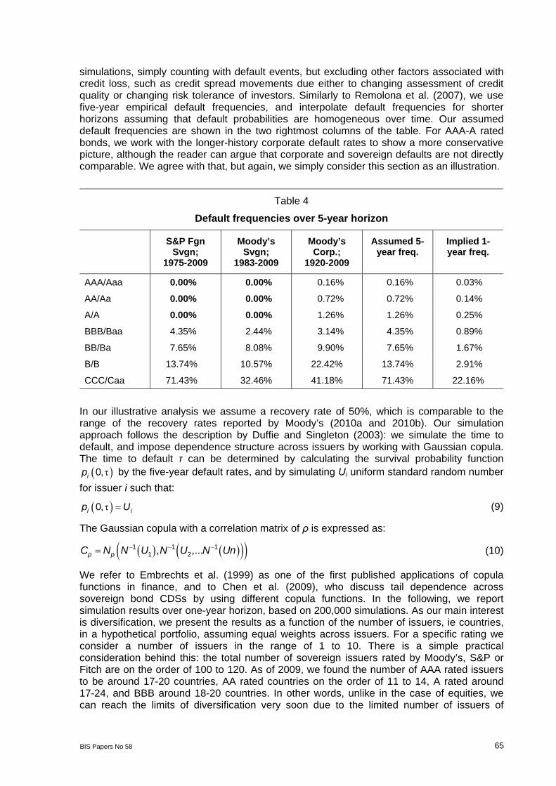
Table 4 summarizes historical sovereign default frequencies, reported by Standard and Poor’s (2010) and Moody’s (2010a). We also show corporate bond defaults based on significantly longer time series, again collected by Moody’s (2010b). In order to illustrate the possible magnitude of credit losses due to default, we run some naïve credit loss

BIS Papers No 58 65

simulations, simply counting with default events, but excluding other factors associated with credit loss, such as credit spread movements due either to changing assessment of credit quality or changing risk tolerance of investors. Similarly to Remolona et al. (2007), we use five-year empirical default frequencies, and interpolate default frequencies for shorter horizons assuming that default probabilities are homogeneous over time. Our assumed default frequencies are shown in the two rightmost columns of the table. For AAA-A rated bonds, we work with the longer-history corporate default rates to show a more conservative picture, although the reader can argue that corporate and sovereign defaults are not directly comparable. We agree with that, but again, we simply consider this section as an illustration.

Table 4

Default frequencies over 5-year horizon

S&P Fgn Svgn;

1975-2009

Moody’s Svgn;

1983-2009

Moody’s Corp.;

1920-2009

Assumed 5-year freq.

Implied 1-year freq.

AAA/Aaa 0.00% 0.00% 0.16% 0.16% 0.03%

AA/Aa 0.00% 0.00% 0.72% 0.72% 0.14%

A/A 0.00% 0.00% 1.26% 1.26% 0.25%

BBB/Baa 4.35% 2.44% 3.14% 4.35% 0.89%

BB/Ba 7.65% 8.08% 9.90% 7.65% 1.67%

B/B 13.74% 10.57% 22.42% 13.74% 2.91%

CCC/Caa 71.43% 32.46% 41.18% 71.43% 22.16%

In our illustrative analysis we assume a recovery rate of 50%, which is comparable to the range of the recovery rates reported by Moody’s (2010a and 2010b). Our simulation approach follows the description by Duffie and Singleton (2003): we simulate the time to default, and impose dependence structure across issuers by working with Gaussian copula. The time to default τ can be determined by calculating the survival probability function

0,ip by the five-year default rates, and by simulating Ui uniform standard random number

for issuer i such that:

0,i ip U (9)

The Gaussian copula with a correlation matrix of ρ is expressed as:

1 1 11 2, ,...p pC N N U N U N Un (10)

We refer to Embrechts et al. (1999) as one of the first published applications of copula functions in finance, and to Chen et al. (2009), who discuss tail dependence across sovereign bond CDSs by using different copula functions. In the following, we report simulation results over one-year horizon, based on 200,000 simulations. As our main interest is diversification, we present the results as a function of the number of issuers, ie countries, in a hypothetical portfolio, assuming equal weights across issuers. For a specific rating we consider a number of issuers in the range of 1 to 10. There is a simple practical consideration behind this: the total number of sovereign issuers rated by Moody’s, S&P or Fitch are on the order of 100 to 120. As of 2009, we found the number of AAA rated issuers to be around 17-20 countries, AA rated countries on the order of 11 to 14, A rated around 17-24, and BBB around 18-20 countries. In other words, unlike in the case of equities, we can reach the limits of diversification very soon due to the limited number of issuers of

66 BIS Papers No 58

sovereign bonds. In Appendix 3 we provide a detailed simulation report, but here we focus only on conditional value-at-risk (CVaR) as the relevant risk measure. CVaR with confidence level α, also known as expected shortfall (ES), quantifies the expected magnitude of loss if we exceed the highest expected loss, ie VaR, estimated at a confidence level α over the selected measurement horizon:

' 'a aCVaT w E r w r w VaR (11)

We use CVaR because, unlike shortfall probability or VaR, it is a coherent measure of risk, as shown, for example, by Acerbi and Tasche (2001). Practically, this means that the risk of a portfolio measured by a coherent measure cannot exceed the weighted arithmetic average of risks of the individual assets, or in other words, coherent measures of risk recognize diversification. Shortfall probabilities, on the other hand, are not coherent, and credit risk is perhaps the best field to demonstrate it. The reader can also find the simulated probabilities of suffering any default loss as a function of the number of issuers in Appendix 4. As can be seen, the probability of any credit loss increases with the number of issuers – intuitively because if there are many issuers in the portfolio, chances are that a default will be seen sooner than when dealing with a single issuer. While the magnitude of loss is more devastating in the case of a concentrated loss, shortfall probability in this case would clearly argue against diversification.

In Figure 10 we show estimated CVaR for Aaa, Aa, A, and Baa rated bond portfolios from one to 10 issuers at the 99% or 99.99% confidence level, assuming 0 correlation. In the case of the 99% CVaR, only the Baa rated portfolio shows any kind of response to the number of issuers. This is simply because the probability of default is much less than 1% for the higher rated bonds. If we push the frontier to the extreme 1:10,000 confidence level, even Aaa rated bonds show some response, even though their probability of default is a mere 3:10,000. That being said, if this very unlikely outcome materializes, the impact can be severe. Figure 12, in any case, shows that diversification can significantly reduce extreme losses if default events are independent.

Figure 12

CVaRs at different confidence levels

-50%

-45%

-40%

-35%

-30%

-25%

-20%

-15%

-10%

-5%

0%

1 2 3 4 5 6 7 8 9 10

99%

C-V

aR

Number of issuers

Aaa

Aa

A

Baa

-60%

-50%

-40%

-30%

-20%

-10%

0%

1 2 3 4 5 6 7 8 9 10

99.9

9% C

-VaR

Number of issuers

Aaa

Aa

A

Baa

In Figure 13 we focus on 99.9% CVaRs of Baa rated bond portfolios only, but impose different degrees of dependence in the copula structure represented by 0.0, 0.3, and 0.5 correlations. CVaR still provides evidence for diversification, although at a decreasing rate with increasing correlations. In reality, we do not think that a uniform correlation would make sense across, say, 10 issuers. Instead, we could think of scenarios such that some countries become more correlated within a cluster, but less correlated with other clusters, as in the case of geographical regions, or the periphery versus the core within the Eurozone. We note that Chen et al. estimate Gaussian copula correlations on the order of 0.7 between

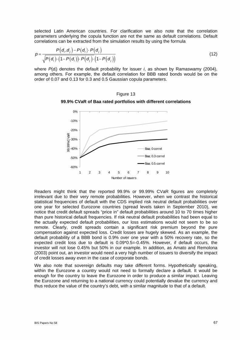
BIS Papers No 58 67

selected Latin American countries. For clarification we also note that the correlation parameters underlying the copula function are not the same as default correlations. Default correlations can be extracted from the simulation results by using the formula

,

1 1

i j i j

i i j j

P d d P d P dp

P d P d P d P d

(12)

where P(di) denotes the default probability for issuer i, as shown by Ramaswamy (2004), among others. For example, the default correlation for BBB rated bonds would be on the order of 0.07 and 0.13 for 0.3 and 0.5 Gaussian copula parameters.

Figure 13

99.9% CVaR of Baa rated portfolios with different correlations

-60%

-50%

-40%

-30%

-20%

-10%

0%

1 2 3 4 5 6 7 8 9 10

99.9

9% C

-VaR

Number of issuers

Baa; 0 correl

Baa; 0.3 correl

Baa; 0.5 correl

Readers might think that the reported 99.9% or 99.99% CVaR figures are completely irrelevant due to their very remote probabilities. However, when we contrast the historical statistical frequencies of default with the CDS implied risk neutral default probabilities over one year for selected Eurozone countries (spread levels taken in September 2010), we notice that credit default spreads “price in” default probabilities around 10 to 70 times higher than pure historical default frequencies. If risk neutral default probabilities had been equal to the actually expected default probabilities, our loss estimations would not seem to be so remote. Clearly, credit spreads contain a significant risk premium beyond the pure compensation against expected loss. Credit losses are hugely skewed. As an example, the default probability of a BBB bond is 0.9% over one year with a 50% recovery rate, so the expected credit loss due to default is 0.09*0.5=-0.45%. However, if default occurs, the investor will not lose 0.45% but 50% in our example. In addition, as Amato and Remolona (2003) point out, an investor would need a very high number of issuers to diversify the impact of credit losses away even in the case of corporate bonds.

We also note that sovereign defaults may take different forms. Hypothetically speaking, within the Eurozone a country would not need to formally declare a default. It would be enough for the country to leave the Eurozone in order to produce a similar impact. Leaving the Eurozone and returning to a national currency could potentially devalue the currency and thus reduce the value of the country’s debt, with a similar magnitude to that of a default.

68 BIS Papers No 58

Figure 14

CDS implied risk neutral probabilities of default versus rating-based frequencies

0.0%

0.2%

0.4%

0.6%

0.8%

1.0%

1.2%

1.4%

1.6%

1.8%

0%

5%

10%

15%

20%

25%

Aus

tria

Belg

ium

Finl

and

Fran

ce

Ger

man

y

Gre

ece

Irel

and

Italy

Net

herl

ands

Port

ugal

Spai

n Ratin

g-ba

sed

freq

uenc

y of

def

ault

CDS-

impl

ied

prob

. of d

efau

lt

1-year CDS implied probability Rating-based frequency

4. Conclusions

The aspects of diversification have become broader over the past years in the context of sovereign bond investments. In the traditional sense, diversification would primarily be considered in terms of volatility reduction. However, mitigating the impact of possible distress became part of the considerations.

In this paper we first discussed global governments from a broad international rate diversification perspective. By looking at the correlations and historical reduction in volatility, we noticed that global high grade sovereign bonds became largely integrated over the past decade. However, global governments did not become an entirely global asset class that is uniformly priced to the same factors. Local factors still have a considerable impact on returns, and the fact that local factors matter makes the fundamental case for diversification prevail. We found that local factors explain around 20-25% of total risk premia, and the volatility historically could have been reduced by 10-30% compared to the average volatility of the G7 countries based on historical observations. It is also important to note that while local factors in Japan became less significant recently, other countries in Europe showed the opposite dynamics.

Second, we discussed sovereign credit risk as this topic has become a key concern in Eurozone government bond markets. The Eurozone underwent a regime switch as recent volatilities and correlations vastly differ from their historical values. Considering diversification from the perspective of default risk, historical analysis does not provide too much insight. We rely on long-term historical default rate data, and ran a naïve hypothetical simulation with different correlation assumptions. Due to the limited number of issuers, diversification does not eliminate default impact, but at least mitigates losses. Also, sovereign default does not have to be a formal default; within the Eurozone context, leaving the euro and returning to a national currency would have a similar impact, as CDS levels show.

We can draw a couple of practical conclusions from the credit risk aspect. First, when an investor decides on the eligible issuers and constituents of the investment benchmark, sovereign credit risk cannot be ignored. The investor needs to own the decision and feel comfortable, whether the specific issuer is part of the benchmark or simply eligible for active management. Regarding the benchmark composition, the allocation weights to specific

BIS Papers No 58 69

countries also matter. Market capitalization weights are typically used by investors; however, market weight increases with increasing indebtedness of an issuer. If credit risk is a concern, we understand considering weighting approaches that penalize the market weights of issuers with increasing credit risk based on qualitative considerations. Finally, the lower we go in the credit ratings, we believe that diversification becomes more and more valuable in mitigating potential losses due to financial distress.

We see several opportunities for further research. One is to bring the two parts presented in this paper to a more common ground, ie measuring interest rate and default risk diversification jointly. Also, some parts of the paper may be developed further as well. Bekaert and Harvey (1995) presented their CAPM-based approach in a regime switching context that would be a natural extension to the Eurozone countries. Finally, understanding sovereign credit risk and its implications for portfolio management remains a very timely issue; clearly many researchers are devoting their efforts to this topic.

70 BIS Papers No 58

Appendix 1: Structure of G7 and Eurozone government markets

Structure of G7 sovereign bond market

As of June 30, 2010 History

USA35%

Canada2%UK

7%Germany7%

France7%

Italy7%

Japan35%

0%

10%

20%

30%

40%

50%

60%

70%

80%

90%

100%

6/1/

2000

2/1/

2001

10/1

/200

1

6/1/

2002

2/1/

2003

10/1

/200

3

6/1/

2004

2/1/

2005

10/1

/200

5

6/1/

2006

2/1/

2007

10/1

/200

7

6/1/

2008

2/1/

2009

10/1

/200

9

6/1/

2010

Japan

Italy

France

Germany

UK

Canada

USA

Structure of Eurozone sovereign bond market

As of May 31, 2010 History

Austria3.8% Belgium

5.9%Finland

1.2%

France20.7%

Germany21.8%

Ireland2.1%

Italy22.9%

Netherlands5.6%

Portugal2.2%

Spain9.1%

Slovakia0.3%

Greece4.3%

0.0%10.0%20.0%30.0%40.0%50.0%60.0%70.0%80.0%90.0%

100.0%

6/1/

2001

2/1/

2002

10/1

/200

2

6/1/

2003

2/1/

2004

10/1

/200

4

6/1/

2005

2/1/

2006

10/1

/200

6

6/1/

2007

2/1/

2008

10/1

/200

8

6/1/

2009

2/1/

2010

Greece

Spain

Portugal

Netherlands

Italy

Ireland

Germany

France

Finland

Belgium

Austria

BIS

Papers N

o 58 71

Appendix 2: Regime-dependent statistics

Austria Belgium Finland France Germany Ireland Italy Nether. Portugal Spain Greece Total

Average return 9.60% 8.52% 9.12% 9.24% 9.36% 6.12% 6.48% 9.84% 4.32% 5.52% -5.52% 7.47%

Ret. over Germany 0.24% -0.84% -0.24% -0.12% - -3.24% -2.88% 0.48% -5.04% -3.84% -14.88% -1.89% Regime 1

Volatility 5.15% 4.41% 3.96% 4.91% 4.80% 6.78% 3.85% 4.77% 7.40% 4.90% 14.88% 4.30%

Average return 4.44% 4.56% 4.44% 4.44% 4.44% 4.20% 4.80% 4.32% 4.32% 4.44% 4.68% 4.53%

Ret. over Germany 0.00% 0.12% 0.00% 0.00% - -0.24% 0.36% -0.12% -0.12% 0.00% 0.24% 0.09% Regime 2

Volatility 3.74% 3.67% 3.22% 3.62% 3.53% 4.88% 3.79% 3.53% 3.53% 3.78% 3.64% 3.63%

Correlation matrices Austria Belgium Finland France Germany Ireland Italy Netherlands Portugal Spain Greece

Austria 1

Belgium 0.95 1

Finland 0.92 0.92 1

France 0.94 0.96 0.95 1

Germany 0.90 0.90 0.97 0.98 1

Ireland 0.73 0.72 0.53 0.59 0.48 1

Italy 0.81 0.81 0.70 0.74 0.67 0.72 1

Netherlands 0.95 0.94 0.96 0.98 0.97 0.59 0.79 1

Portugal 0.60 0.65 0.48 0.54 0.45 0.88 0.57 0.51 1

Spain 0.71 0.79 0.63 0.72 0.65 0.71 0.90 0.71 0.67 1

Regime 1

Greece 0.30 0.33 0.15 0.21 0.11 0.75 0.26 0.16 0.90 0.40 1

Austria 1

Belgium 1.00 1

Finland 0.97 0.98 1

France 1.00 1.00 0.97 1

Germany 1.00 1.00 0.98 1.00 1

Ireland 0.92 0.92 0.86 0.92 0.90 1

Italy 0.98 0.98 0.96 0.98 0.98 0.84 1

Netherlands 1.00 1.00 0.98 1.00 1.00 0.93 0.97 1

Portugal 0.99 0.99 0.97 0.99 0.98 0.95 0.95 0.99 1

Spain 0.99 0.99 0.96 0.99 0.99 0.96 0.96 0.99 0.99 1

Regime 2

Greece 0.99 0.99 0.98 0.99 0.99 0.91 0.98 0.99 0.98 0.98 1

72

BIS

Papers N

o 58

Appendix 3: Credit simulation results

Pairwise correl=0 Pairwise correl=0.3 Pairwise correl=0.5

# Issuers 1 3 5 10 1 3 5 10 1 3 5 10

Aaa -0.02% -0.02% -0.02% -0.02% -0.02% -0.02% -0.02% -0.02% -0.02% -0.02% -0.02% -0.02%

Aa -0.07% -0.07% -0.07% -0.07% -0.07% -0.07% -0.07% -0.07% -0.07% -0.07% -0.07% -0.07%

A -0.13% -0.13% -0.13% -0.13% -0.13% -0.13% -0.13% -0.13% -0.13% -0.13% -0.13% -0.13%

Exp

ecte

d Lo

ss

Baa -0.45% -0.45% -0.45% -0.45% -0.45% -0.45% -0.45% -0.45% -0.45% -0.45% -0.45% -0.45%

Aaa 0.03% 0.10% 0.17% 0.33% 0.03% 0.10% 0.17% 0.35% 0.03% 0.08% 0.13% 0.25%

Aa 0.15% 0.42% 0.73% 1.43% 0.15% 0.44% 0.71% 1.37% 0.15% 0.40% 0.64% 1.13%

A 0.26% 0.75% 1.27% 2.51% 0.26% 0.75% 1.24% 2.33% 0.26% 0.69% 1.07% 1.90%

Pro

b. o

f cre

dit

loss

Baa 0.87% 2.59% 4.30% 8.42% 0.87% 2.52% 4.06% 7.40% 0.87% 2.18% 3.31% 5.61%

Aaa -1.7% -1.6% -1.6% -1.6% -1.7% -1.7% -1.7% -1.7% -1.7% -1.5% -1.5% -1.5%

Aa -7.5% -7.3% -7.1% -5.0% -7.5% -7.5% -7.3% -5.5% -7.5% -7.1% -7.1% -6.2%

A -12.8% -12.6% -10.1% -5.1% -12.8% -12.7% -10.6% -6.2% -12.8% -12.2% -11.5% -7.4%

99%

CV

aR

Baa -43.5% -17.0% -10.8% -6.6% -43.5% -19.0% -14.1% -11.9% -43.5% -21.2% -17.6% -15.1%

Aaa -17.0% -15.8% -10.0% -5.0% -17.0% -16.8% -10.2% -5.6% -17.0% -15.0% -11.3% -6.8%

Aa -50.0% -16.8% -10.2% -5.4% -50.0% -18.4% -12.4% -9.6% -50.0% -20.1% -17.0% -13.7%

A -50.0% -16.8% -10.7% -6.3% -50.0% -21.3% -16.4% -11.6% -50.0% -23.6% -22.9% -18.2%

99.9

% C

VaR

Baa -50.0% -19.9% -16.5% -10.4% -50.0% -32.3% -24.8% -19.4% -50.0% -38.6% -34.0% -29.8%

Aaa -50.0% -16.7% -10.0% -5.3% -50.0% -18.3% -12.0% -10.3% -50.0% -25.8% -23.0% -16.3%

Aa -50.0% -18.3% -12.0% -9.0% -50.0% -33.3% -20.5% -15.0% -50.0% -36.7% -32.0% -27.8%

A -50.0% -20.3% -16.0% -10.0% -50.0% -34.2% -23.0% -17.8% -50.0% -40.0% -35.0% -32.5%

99.9

9% C

VaR

Baa -50.0% -35.0% -22.0% -13.8% -50.0% -43.3% -35.5% -27.0% -50.0% -50.0% -46.5% -43.3%

BIS Papers No 58 73

References

Abad, P., Chuila, H., Gomez-Puig, M. (2009): EMU and European Government Bond market Integration, ECB Working Paper No. 1079.

Acerbi, C., Tasche, D. (2001): Expected Shortfall: a natural coherent alternative to Value at Risk; Working Paper.

Amato, J. D.,Remolona, E. M. (2003):M The credit spread puzzle, BIS Quarterly Review, December 2003.

Arnott, Robert D., Jason C. Hsu, and Philip Moore. 2005. Fundamental indexation. Financial Analysts Journal 61(2): 83-99.

Arnott, Robert D., Jason C. Hsu, Feifei Li, and Shane D. Shepherd. Spring 2010. Valuation-indifferent weighting for bonds. The Journal of Portfolio Management Vol 36 Number 3.

Barr, D. G., Priestley, R. (2004): Expected returns, risk and the integration of international bond markets, Journal of Intenrational Money and Finance, Vol. 23., pp 71-97.

Bekaert, G., Harvey, C. (1995): Time-Varying World Market Integration, The Journal of Finance, VOl. L. No. 2.

Barclays Capital (2009): Global Family of Indices; Barclays Capital Index Products, November 2009.

Chen, Y., Wang, K., Tu, A. H. (2009): Default correlation at the sovereign level: evidence from Latin American markets; in: Applied Economics, ed. Mark Taylor, Routledge, London.

Duffie, D., Singleton, K. J. (2003): Credit Risk, Princeton Series in Finance, Princeton University Press.

Dynkin, L. & Ben Dor A. (2006). Issuer capped sovereign indices, Fixed Income Research, Lehman Brothers.

Embrechts, P., McNeil, A., Strauman, D. (1999): Correlation and Dependence in Risk Management: Properties and Pitfalls. ETHZ Working paper.

Gray, D., Malone, S. (2008): Macrofinancial Risk Analysis; Wiley Finance.

Hamilton, J. D. (1990): Analysis of Time Series Subject to Changes in Regime. Journal of Econometrics, Vol. 45, No. 1-2, pp. 39-70.

Hamilton, J. D. (1994) Time Series Analysis. New Jersey, NJ: Princeton University Press.

Kim, C. and Nelson, C. R. (1999): State-Space Models with Regime Switching—Classical and Gibbs-Sampling Approaches and Applications. Cambridge, MA: MIT Press.

Longstaff, F. A., Pan, J., Pedersen, L. H., Singleton, K. J. (2008): How sovereign is sovereign credit risk?, conference paper for 5th Annual Credit Risk Conference, Moody’s Corp. amd NYU Stern School of Business.

Moody’s (2010a): Sovereign Default and Recovery Rates, 1983-2009; Moody’s Investor Service, April 2010.

Moody’s (2010b): Corporate Default and Recovery Rates, 1920-2009; Moody’s Investor Service, February 2010.

PIMCO (2010): PIMCO Global Advantage Government Bond Index.

Ramaswamy, S. (2004): Managing credit risk in corporate bond portfolios – a practitioner guide. Wiley Finance.

Remolona, E. M., Scatina, M., Wu, E. (2007): Interpreting sovereign spreads, BIS Quarterly Review, March 2007.

74 BIS Papers No 58

Reinhart. C. M., Rogoff K. S. (2009): This Time is Different – Eight Centuries of Financial Folly, Princeton University Press.

Siegel, L. B. (2003): Benchmarks and Investment Management. The Research Foundation of the AIMR.

Standard and Poor’s (2010): Sovereign Defaults and Rating Transition Data, 2009 Update; Standard and Poor’s, March 17, 2010.

Wei, J. Z. (2003): A multi-factor, credit migration model for sovereign and corporate debts. Journal of International Money and Finance 22.

Winkelmann, K. (2003): International Diversification and Currency Hedging, in. Modern Investment Management – An equilibrium approach, ed. Litterman, B., John Wiley & Sons, New Jersey.