Diversification, Productivity, and Financial Constraints:

Empirical Evidence from the US Electric Utility Industry

Mika Goto

Central Research Institute of Electric Power Industry

Angie Low

Nanyang Business School, Nanyang Technological University

Anil K. Makhija*

Fisher College of Business, The Ohio State University

This Version: February 28, 2008

________________________________________________________________________________

Abstract

We examine the real effects of parent firm diversification on their electric utility operating

companies over the period, 1990-2003. Since electric utility operating companies produce a single

homogenous product, we can better measure their Total Factor Productivity and make valid

comparisons of productivity across firms. We find that, consistent with a diversification discount,

greater parent diversification is associated with lower productivity across electric utility operating

companies. However, the productivity of the electric utility operating companies improves with

greater parent diversification over time. Diversification appears to provide an alternative channel

to divert investment dollars away from overinvestment in the core electric business. Finally, we find

that the improvement in the productivity of the electric utility operating companies from greater

parent firm diversification over time is limited to financially constrained firms. This suggests that

when managers have no resources to waste, it is more likely that any diversification activities are

carefully planned and undertaken for strategic purposes that can help to increase productivity of the

core business.

Key words: Diversification, Total Factor Productivity, Financial Constraints, Electric Utilities

JEL Classification Code: L25, L94

________________________________________________________________________________

* Corresponding author: Anil K. Makhija, Rismiller Professor of Finance, Fisher College of Business, The Ohio State University, 2100 Neil Avenue, Columbus, OH 43210. E-mail: makhija_1@fisher.osu.edu.

- 1 -

1. Introduction

There is a vast literature on how diversification affects the market values of firms. Following

Lang and Stulz (1994) and Berger and Ofek (1995), many studies have documented that diversified

firms sell at a discount relative to the sum of the values of their stand-alone component segments.

Conglomerates earn lower stock market returns, according to Comment and Jarrell (1985). The

implication is that diversification destroys corporate value. However, Campa and Kedia (2002) and

Villalonga (2004) argue that the diversification discount arises endogenously. They find that

diversifying firms tend to trade at a discount even before they diversify, while Graham, Lemmon, and

Wolf (2002) document that conglomerates tend to purchase already discounted target firms.

Confounding the issue further, Villalonga (2004) points out that the conglomerate discount is a result of

data biases in the Compustat segment data, which are commonly used in research on the diversification

discount. Given this controversy surrounding how diversification affects market valuations, a strand of

research has begun a new approach by examining the real effects of diversification. In a limited

literature so far, Schoar (2002) and Maksimovic and Phillips (2002) have both used plant-level data from

the U.S. Census Bureau on manufacturing firms to study how diversification affects plant productivity.

In this paper, we extend this line of inquiry by examining how the productivity of U. S. electric utility

operating companies was affected by the diversification decisions of their parent firms during the period,

1990 to 2003. We also examine how the parent’s financial constraints affect the relationship between

its diversification and the productivity of its electric utility operating company. This financing aspect

has not been addressed before.

There are several reasons to study the real effects of diversification on electric utility operating

companies, going beyond the contradictory findings based only on manufacturing firms with additional

evidence from another important industry. While Schoar (2002) reports that more diversified firms

have higher productivity, according to Maksimovic and Phillips (2002) conglomerate firms are less

productive than single-segment firms because of the significantly lower productivity of peripheral

divisions relative to the main divisions. The electric utility industry offers fertile ground for additional

- 2 -

evidence because it has engaged in substantial amounts of diversification (57% of all utilities were

engaged in non-electric businesses by 1997, Jandik and Makhija, 2005). The greater issue here,

however, is the manner in which earlier studies estimate productivity, the main criterion for assessing the

impact of diversification. As Schoar (2002) herself acknowledges, their estimate of Total Factor

Productivity (TFP) is determined by approximating output by the value of total shipments and changes

in value of inventory. Thus, their TFP reflects not only the desired variations in efficiency but also

differences in markups. The problem, of course, lies in the difficulty in formulating physical output

across a sample of manufacturing firms with heterogeneous products. The heterogeneity of products

also implies that their TFP measures are not truly comparable across the firms. In contrast, electric

utility operating companies produce a single, homogenous product, measured in megawatt-hours of

electricity.

Even as we make a case for reexamining the impact of diversification on productivity, we do not

hypothesize a specific impact. Instead, we argue that the impact of parent diversification on the

productivity of the operating company is an empirical issue. It has been claimed that diversification

has adverse effects because internal capital markets allocate capital sub-optimally across divisions

(Rajan, Servaes, and Zingales, 2000, Scharfstein and stein, 2000, Scharfstein, 1998, and Shin and Stulz,

1998). On the other hand, Alchian (1969), Weston (1970), Williamson (1975), Gertner, Scharfstein,

and Stein (1994), and Stein (1996) stress the benefits and positive impact of internal capital markets.

Since the electric utility operating company is invariably the core and major business of the parent

firm, the electric utility industry also presents a suitable setting to assess the impact of the parent’s

financial condition on how its diversification affects the productivity of its operating company. If the

financial condition of the parent firm determines the “financial slack” to underwrite

productivity-enhancing investments by the electric utility operating company, we expect that for

financially unconstrained parent firms the relation between parent diversification and operating company

productivity will at least not be adversely affected. However, financial slack can also worsen the

diversification-productivity relationship. When managers have relatively more resources than

- 3 -

investment opportunities, the diversification activities are likely to be “pet projects” that distract

managers from their core business, leading to reductions in productivity. This is a relevant concern for

the electric utility industry. Many parent firms in the industry historically can be characterized as

having low growth and high free cash flows. These are just the type of firms in which Jensen (1986)

has argued that managers tend to overinvest in self-serving negative net present value projects. This

raises the possibility that diversifying activities were undertaken by many utility managers for

empire-building and entrenchment purposes, all of which take away attention from the main business of

the firm. Indeed, diversification is often argued to be a result of overinvestment (Morck, Shleifer, and

Vishny (1990)). Acquisitions by cash-rich, low-growth firms perform worse than those of other

acquirers (Lang, Stulz, and Walkling (1991)). Similarly, Denis, Denis, and Sarin (1997) find that

managerial agency problems explain why firms maintain value-destroying diversification strategies.

Consistent with the agency cost of free cash flow, Harford (1999) finds that cash-rich firms are more

likely to undertake diversifying acquisitions. Notably, in his review of the investments literature, Stein

(2003) stresses that value-destroying over-investments occur only when the level of free cash flow

relative to investment opportunities is greater than expected. Similarly, there are competing explanations

on how diversification matters for the financially constrained firm. Greater diversification by a

financially constrained firm diverts available dollars from productivity-enhancing investments. On the

other hand, when managers are constrained and have no extra resources to waste, it is likely that any

diversification activities are undertaken for strategic purposes and therefore help to increase productivity

at the core business. Moreover, when managers are constrained, they often have to go to the external

capital markets for funding and this extra monitoring from the capital markets prevents managers from

engaging in value-destroying activities. This tri-lateral relation between productivity, diversification, and

financial conditions has been ignored in previous work on the real effects of diversification.

We form a matched panel dataset of electric operating companies and their corresponding parent

companies for the 1990-2003 the period. We then relate the productivity of the operating companies to

diversification activities and financial conditions at the parent company. First, we examine the

- 4 -

relationship between operating company TFP and a number of measures of parent diversification

(number of segments, sales herfindahl, asset herfindahl, and fraction of non-utility sales). We study the

cross-sectional (Fama-MacBeth estimations) and time-series (operating company fixed effects)

relationships. Contrary to Schoar (2002), we find that in the cross-section, more diversified parents are

associated with less productive operating companies, but, in the time series, diversifying activities

increase the productivity of the core electric utility segment. The cross-sectional findings support the

diversification discount reported by Lang and Stulz (1994) and Berger and Ofek (1995). Our results are

also consistent with Maksimovic and Phillips (2002) who use plant-level data and find that diversified

firms are less productive than single-segment firms. They argue that when firms have relative

comparative advantage across industries, it might be optimal for less efficient firms to diversify. As for

the beneficial impact of diversification over time, it is consistent with the explanation offered by Jandik

and Makhija (2005). Diversification has provided cash-rich utilities a channel for diverting investment

dollars that would have otherwise led to unproductive over-investment in the core electric business.

Next, we examine how the parent firm’s financial condition affects the productivity impact of

diversification. To take into account both the financial conditions and growth prospects, we make use

of the KZ-index (Kaplan and Zingales, 1997), which measures the degree of financial constraints faced

by a firm, taking into account the cash flows generated, cash on hand, leverage ratios, dividend

payments, and growth opportunities. Our findings are unchanged when we use the coverage ratio

instead of KZ. Consistent with Jensen’s (1986) agency costs of free cash flow, we find that

diversification undertaken when the parent faces financial slack has a negative impact on productivity at

the operating company. However, diversification undertaken when the parent company is financially

constrained has a positive impact on the electric segment productivity. These results indicate that

financially constrained firms undertake diversifications more carefully, such that they have a beneficial

effect on the core business. Further, when managers are constrained, they often have to go to the

external capital markets for funding and this extra monitoring from the capital markets prevents

managers from engaging in productivity-destroying activities.

- 5 -

The remaining structure of this paper is organized as follows: Section 2 briefly reviews the

literature on diversification and describes the deregulation activities in the utility industry. Section 3

describes the data, the variables used, and the methodology. The results are presented in Section 4.

Section 5 concludes and discusses future agendas.

2. Literature Review on Diversification and the Regulatory Background

2.1. Literature Review

Several papers have documented that conglomerates trade at a discount relative to single-segment

firms in the same industry. They do this by comparing the market value of conglomerates to the value

of a portfolio of focused firms operating in the same industries as the conglomerate’s divisions. Using

this approach, Lang and Stulz (1994) find that diversified firms have lower values of Tobin’s Q

compared to single-segment firms. In another study, Berger and Ofek (1995) find that U.S.

conglomerates trade at a discount of 15%. Other papers have confirmed this finding using different

sample periods and different countries. For example, Servaes (1996) finds a discount for

conglomerates during the 1960s, Lins and Servaes (1999, 2002) document significant discounts in Japan,

the United Kingdom, and a sample of firms from seven emerging markets.1

However, recent literature contests the interpretation that diversification destroys firm value.

Instead, papers such as Campa and Kedia (2002) and Villalonga (2004) argue that the diversification

discounts arises endogenously. They find that diversifying firms tend to trade at a discount even before

they diversify, while Graham, Lemmon, and Wolf (2002) document that conglomerates tend to purchase

already discounted target firms. Maksimovic and Phillips (2002) propose a neo-classical,

profit-maximizing model where firms optimally choose the number of segments they operate in

depending on their comparative advantage. Other studies have also contested the validity of the

conglomerate discount, arguing that Compustat segment data is biased towards finding a conglomerate

1 However, Matsasuka (1993) documents gains to diversifying acquisitions during the 1960s, and Khanna and Palepu (2000) and Fauver, Houston, and Naranjo (1998) do not find evidence of discounts in emerging markets.

- 6 -

discount (see e.g., Villalonga (2004)).

Pertinent to our study, a few papers study the real effects of diversification as an alternative

approach to simply looking at market valuations. Using plant-level data from the U.S. Census Bureau,

Schoar (2002) documents that diversified firms are on average more productive than focused firms.

However, productivity at incumbent plants falls when firms diversify. This is mainly attributed to neglect,

as management turns its attention to the newly-acquired division. Using the same source of data,

Maksimovic and Phillips (2002) find that conglomerates are less productive, especially in their

peripheral segments, consistent with the model of profit maximization they propose. They also find

that firms allocate resources efficiently across the different industry segments. In examining changes in

productivity during asset reallocations, Maksimovic and Phillips (2001) find that on average,

productivity gains accompany such transactions. However, the gains depend on the productivity of the

acquiring firm and whether it is the main or peripheral division. The authors, however, cannot rule out

agency considerations that may drive some transactions.

The studies on the real effects of diversification have the benefit of a large sample of

manufacturing firms. However, the manufacturing industry is very diverse and comparisons of

productivity across firms are problematic given that the firms have very different products.

Consequently, in this study we examine firms producing a single, homogenous product – electricity.

By studying the electric utility industry only, we are able to control for the product heterogeneity,

therefore allowing for a more precise measurement and comparison of productivity across firms.

Furthermore, most studies on diversification have ignored the electric utility industry, primarily because

of the heavy regulation in the industry. However, deregulation efforts during the 1980s and early 1990s

imply that for most of the 1990s, the managers in the electric utility industry did have considerable

discretion in their diversification and investment projects, similar to firms in other industries. At any

rate, as a robustness test we take into account the ease of state-level diversification policies.

Since the core business of the electric utilities is the same, we are able to effectively control for

the industry conditions and examine how diversification into non-related businesses affects the

- 7 -

productivity in the incumbent segments. Furthermore, we seek to understand under what conditions

would diversification be beneficial and when it would not. Specifically, we concentrate on the motives

managers may have when they diversify. An influential view in the literature is that there are conflicts

of interest between managers and shareholders and that can result in investment decisions being taken

for the private benefits of managers (Jensen and Meckling (1976), Jensen (1986, 1993)), including

diversifying activities that are undertaken for empire-building and managerial entrenchment purposes.

Indeed, Morck, Shleifer, and Vishny (1990) find poor announcement returns for acquirers who engage in

diversifying acquisitions. Denis, Denis, and Sarin (1997) also find evidence that managerial agency

issues are responsible for firms maintaining value-destroying diversification strategies.

Managers may seek diversification because of the prestige and increased compensation associated

with running bigger firms. Jensen’s (1986) agency theory of free cash flow predicts that when the level

of internal firm resources relative to investment opportunities is higher than expected, managers tend to

overinvest and that the diversification undertaken under such conditions is likely to be value-destroying.

Consistent with this, Lang, Stulz, and Walkling (1991) find that the acquisitions of cash-rich, low-growth

firms perform worse, and Harford (1999) documents that cash-rich firms are more likely to undertake

diversifying acquisitions. However, Stein (2003) stresses the fact that not all firms are empire-building,

and that in only some states of the world would value-destroying overinvestment be present. Based on

Jensen’s (1986) theory, we do not hypothesize that all diversifications are efficiency-reducing, rather

only the diversifications undertaken by firms with financial slack and with relatively low growth are

likely to have a negative impact on productivity.

2.2. Regulatory Background

Although the Public Utility Holding Company Act (PUHCA) passed in 1935, gave the SEC the

authority to limit diversification activities by utilities “to such other businesses as are reasonably

incidental, or economically necessary or appropriate” to the operations of the utility, in reality most

utilities were successful in avoiding this law by forming exempt holding companies. The exemption was

- 8 -

readily granted if the operating utility and non-utility companies of a parent were organized to operate

within the jurisdiction of a single state-level Public Utility Commission (PUC). In fact, the regulation

of diversification has long come under the purview of state-level PUC’s. Further deregulation was

enacted through The Energy Policy Act of 1992 (EPACT), which permitted the formation of unregulated

generation plants and sale at wholesale prices. In general, with a passage of EPACT there was a change

in the mindset regarding the regulation of diversification. Many states developed procedures to

routinely process diversification requests from utilities. Regulators were not concerned about the

profitability (or productivity effects) of diversification, but only with protecting ratepayers from having

to cross-subsidize non-utility businesses in their electricity bills. Since the period of this study,

1990-2003, largely falls after the year 1992, diversification decisions of utilities are not markedly

different from those of other firms. Nevertheless, in our analysis we control for the ease of state-level

regulation of diversification.

3. Data and Methodology

The data are obtained from a number of sources. Data on the electric utilities are obtained from

Federal Energy Regulation Commission (FERC) Form 1 supplemented with data from POWERdat.

FERC Form 1 is the Annual Report of Major Electric Utilities, downloadable from

http://www.ferc.gov/docs-filing/eforms.asp. FERC Form 1 contains financial and operational

information filed by the electric utilities themselves. POWERdat, a comprehensive database for the

electric utilities industry, is provided by Platts, a division of McGraw-Hill Companies, Inc.

POWERdat provides detailed historical information on over 5,000 electric power companies, their

plants and even down to their units. The information provided includes production costs, operation

costs, financial data, investment outlays, electricity sales, fuel supply, rates, wholesale power

transactions, etc. The level of detail allows us to estimate the productivity of the utilities very

precisely. The sample consists of 1,736 firm-year observations for 124 investor-owned electric power

utilities (electric utility operating companies) in the U.S. during the period from 1990 through 2003.

- 9 -

The operating companies are required to have total retail sales volume of more than 100,000 Mega Watt

hours (MWh) per year. Companies which are not involved in the retail business, such as those that are

solely in the generation business or wholesale electricity business, are therefore excluded.

We match each operating company to its parent company using information from company

websites and company 10-K filings. Changes in ownership of the operating company are obtained

from these sources as well. Sometimes, the parent is acquired and we check through the Mergers and

Acquisitions database of Securities Data Corporation (SDC) to find such changes in ownership.

Accounting information on the parent companies is then obtained from Compustat.

Insert Table 1 around here.

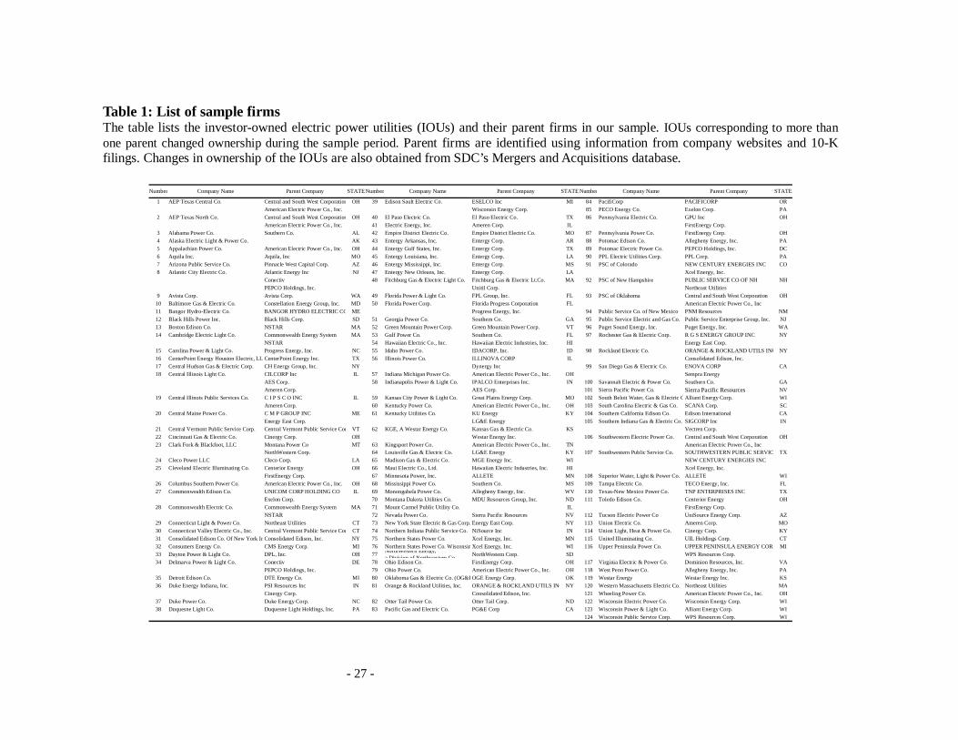
Table 1 provides summary statistics about the operating companies and their corresponding

parents (holding companies) that are included in our sample. The table also provides the states where

the operating companies are located. Operating companies that are associated with more than one

parent are the ones that changed their parent during the sample period. Thus the 122 operating

companies are matched to 98 distinct parents, since 2 operating companies cannot be matched to parent

firms on Compustat during our sample period. The two operating companies are Alaska Electric

Light & Power Co. and Mount Carmel Public Utility Co. The resulting dataset is an unbalanced panel

due to the unavailability of the data for each parent company during each year of our sample period.

3.1. Measuring Productivity - Total Factor Productivity (TFP)

Our primary measure of firm performance is total factor productivity (TFP) of the operating unit.

The production function is specified by a translog functional form, which essentially is a second-order

approximation to the first-order Cobb-Douglas production function. Because it incorporates all

second-order (interaction- or cross-) terms across inputs, it is deemed to be very flexible, allowing for

representation of substitution possibilities without restrictive assumptions about the shape of the

- 10 -

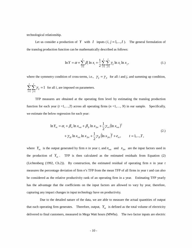
technological relationship.

Let us consider a production of Y with I inputs ( Iji ,...,1, = ). The general formulation of

the translog production function can be mathematically described as follows:

,lnln2

1lnln

1 11ji

I

i

I

jiji

I

ii xxxY ∑∑∑

= ==

++= γβα (1.)

where the symmetry condition of cross-terms, i.e., jiij γγ = for all i and j, and summing up condition,

11 1

=∑∑= =

I

i

I

jijγ for all i, are imposed on parameters.

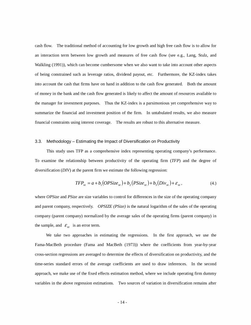
TFP measures are obtained at the operating firm level by estimating the translog production

function for each year (t =1,…,T) across all operating firms (n =1,…, N) in our sample. Specifically,

we estimate the below regression for each year:

( )

( ) ,,...,1 ,ln21

lnln

ln2

1lnlnln

2

2

Ttexxx

xxxY

ntfntfftfntvntvft

vntvvtfntftvntvttnt

=+++

+++=

γγ

γββα (2.)

where ntY is the output generated by firm n in year t, and vntx and fntx are the input factors used in

the production of ntY . TFP is then calculated as the estimated residuals from Equation (2)

(Lichtenberg (1992, Ch.2)). By construction, the estimated residual of operating firm n in year t

measures the percentage deviation of firm n’s TFP from the mean TFP of all firms in year t and can also

be considered as the relative productivity rank of an operating firm in a year. Estimating TFP yearly

has the advantage that the coefficients on the input factors are allowed to vary by year, therefore,

capturing any impact changes in input technology have on productivity.

Due to the detailed nature of the data, we are able to measure the actual quantities of output

that each operating firm generates. Therefore, output, ntY is defined as the total volume of electricity

delivered to final customers, measured in Mega Watt hours (MWhs). The two factor inputs are electric

- 11 -

operation and maintenance (O&M) costs and capital stock. The electric O&M costs include

expenditures for fuel, labor, and purchased power, which are commonly recognized as inputs in the

production of electricity. The O&M cost is converted to real terms using a state-level gross domestic

product (GDP) deflator, obtained from the Bureau of Economic Analysis (BEA), U.S. Department of

Commerce (downloadable from http://www.bea.gov/regional/gsp/). An advantage of using this deflator

is that we can obtain the time series deflators for each state. However, the disadvantage of using such a

deflator is its generality because the GDP by state includes all industries so that influences of other

industries, that are unrelated to the utilities industry, are included in the movement of the index. Finally,

capital stock is constructed using the perpetual inventory method. Capital stock for the base year is

calculated by applying a “triangularized” weighted average procedure proposed by Cowing et al. (1981).

The values of capital stock are then written forward each year with the nominal capital expenditures and

depreciation level obtained from the BEA. Such a procedure helps reduce the impact of potential

accounting manipulations of book values of capital stock. Additional details on the construction of the

capital stock are described in Appendix A.

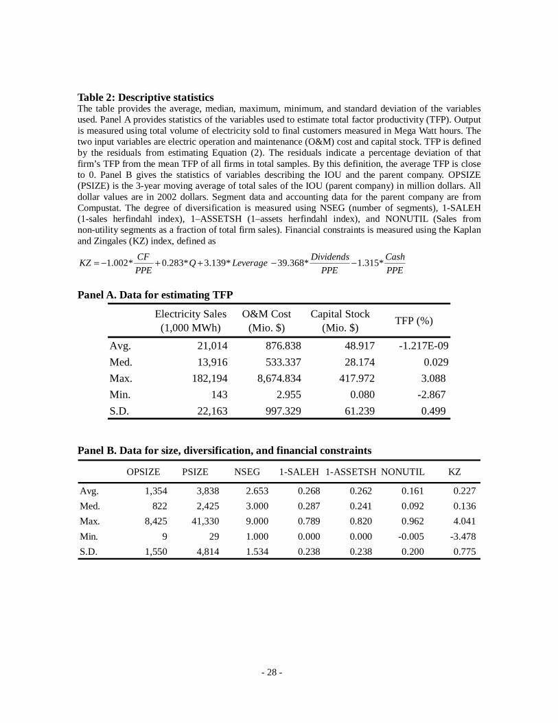
Table 2, Panel A provides the summary statistics of the calculated TFP and the variables used

in the calculation of TFP. By construction, the average TFP is zero since TFPs are the estimated

residuals from yearly regressions. Importantly, there is much variation in the productivity of the

operating firms in our sample as shown by the standard deviation. Therefore, the efficiency of

operating companies differs greatly, allowing us to have a meaningful test of our hypothesis that parent

firm diversification and financial conditions affect the productivity of the operating unit.

Insert Table 2 around here.

3.2. Data on Diversification and Financial Constraints

Our main independent variables which measure the degree of diversification of the parent

company are from the Compustat segment files. We have four measures of diversification. The first

- 12 -

measure is the natural logarithm of number of segments. To take into account the relative size of the

segments, we calculate herfindahl-based measures of diversification. The second and third measures

are the sales herfindahl and asset herfindahl. Sales herfindahl (asset herfindahl) is the sum of the

squares of each segment sales (assets) as a fraction of total sales (assets). For ease of interpretation, we

use (1-sales herfindahl) and (1-asset herfindahl) in our regressions. Therefore, the greater the

diversification, the greater will be the values of (1-sales herfindal) and (1-asset herfindahl). The last

measure of diversification is sales from non-utility segments (with SIC codes other than 4911 and 4931)

as a fraction of total sales2.

Jensen (1986) argues that managers are more likely to undertake value-destroying investments if

they have large amounts of free cash flows under their control. This is especially problematic for low

growth firms which have relatively few positive net present value projects. By using

internally-generated resources as opposed to raising money in the capital markets, managers can escape

the scrutiny of the capital markets, allowing them to invest in wasteful, unprofitable investments. One

such type of investment is investing in businesses that are unrelated to the core businesses. The

negative value premium for diversified firms has often been attributed to managerial agency problems

(see e.g., Denis, Denis, and Sarin (1997)). Harford (1999) finds that cash-rich firms are more likely to

undertake diversifying acquisitions. However, Harford does not examine whether the diversifying

acquisitions undertaken by cash-rich firms have differential performance compared with the diversifying

acquisitions undertaken by non-cash-rich firms. It is therefore unclear whether all diversifying actions

are value-destroying. We hypothesize that diversification undertaken by firms with large amounts of

free resources relative to investment opportunities will perform worse than diversification undertaken by

managers who are constrained by the amount of resources they have, relative to their growth

opportunities.

To measure whether managers have excess internal cash flows for investments in value-destroying

2 SIC code 4911 is Electric Services industry and SIC code 4931 is Electric and other Services Combined industry.

- 13 -

projects, we make use of the financial constraints index developed by Kaplan and Zingales (1997),

henceforth called KZ-index. This measure has been adapted for use in several studies such as Lamont,

Polk, and Saa-Requejo (2001), Baker, Stein, and Wurgler (2003), and Malmendier and Tate (2005),

therefore providing external validity for the KZ-index. Kaplan and Zingales (1997) generate measures

of the degree of financial constraint using quantitative and qualitative information from annual reports to

classify their sample of firms either as financially constrained or financially unconstrained. They then

estimate an ordered logit model on five accounting measures that attempt to capture the degree of

financial constraints: cash flow to net property, plant, and equipment (net PPE), Tobin’s q (Q), leverage

(Leverage), dividends to net PPE (Dividends), and cash holdings to net PPE (CF). Using the

coefficients from their ordered logit regressions, we construct an index of financial constraints as

follows:

.*1.314759*39.3678

*3.139193*0.2826389*1.001909

11

1

−−

−

−−

++−=

it

it

it

it

ititit

itit

PPE

Cash

PPE

Dividends

LeverageQPPE

CFKZ

(3.)

By construction, higher values of the KZ-index indicates more severe financial constraints than

lower values of the KZ-index. Based on the KZ-index, financially constrained firms do not have

enough internally-generated cash flows or cash holdings to meet their investments needs as proxied by

their Tobin’s Q. Furthermore, financially constrained firms have high levels of debt, making it difficult

for them to raise funds further from the debt market. Finally, firms which can afford to pay dividends

are considered not constrained, constrained firms are short on cash and would not pay dividends.

The KZ-index has some attractive features from our perspective. Based on accounting

information, the KZ-index aggregates various dimensions of being constrained into a single metric, thus

allowing for an objective test of the hypothesis and easier interpretation of the results. Furthermore,

Jensen’s empire-building hypothesis applies to firms with low growth and high free cash flow. Thus,

the KZ-index already takes into account the growth opportunities of firms together with the amount of

- 14 -

cash flow. The traditional method of accounting for low growth and high free cash flow is to allow for

an interaction term between low growth and measures of free cash flow (see e.g., Lang, Stulz, and

Walkling (1991)), which can become cumbersome when we also want to take into account other aspects

of being constrained such as leverage ratios, dividend payout, etc. Furthermore, the KZ-index takes

into account the cash that firms have on hand in addition to the cash flow generated. Both the amount

of money in the bank and the cash flow generated is likely to affect the amount of resources available to

the manager for investment purposes. Thus the KZ-index is a parsimonious yet comprehensive way to

summarize the financial and investment position of the firm. In untabulated results, we also measure

financial constraints using interest coverage. The results are robust to this alternative measure.

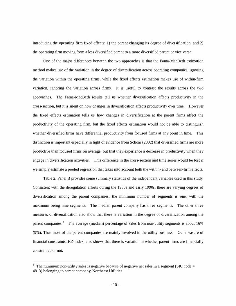
3.3. Methodology – Estimating the Impact of Diversification on Productivity

This study uses TFP as a comprehensive index representing operating company’s performance.

To examine the relationship between productivity of the operating firm (TFP) and the degree of

diversification (DIV) at the parent firm we estimate the following regression:

( ) ( ) ( ) ntntntntnt DivbPSizebOPSizebaTFP ε++++= 321 , (4.)

where OPSize and PSize are size variables to control for differences in the size of the operating company

and parent company, respectively. OPSIZE (PSize) is the natural logarithm of the sales of the operating

company (parent company) normalized by the average sales of the operating firms (parent company) in

the sample, and ntε is an error term.

We take two approaches in estimating the regressions. In the first approach, we use the

Fama-MacBeth procedure (Fama and MacBeth (1973)) where the coefficients from year-by-year

cross-section regressions are averaged to determine the effects of diversification on productivity, and the

time-series standard errors of the average coefficients are used to draw inferences. In the second

approach, we make use of the fixed effects estimation method, where we include operating firm dummy

variables in the above regression estimations. Two sources of variation in diversification remains after

- 15 -

introducing the operating firm fixed effects: 1) the parent changing its degree of diversification, and 2)

the operating firm moving from a less diversified parent to a more diversified parent or vice versa.

One of the major differences between the two approaches is that the Fama-MacBeth estimation

method makes use of the variation in the degree of diversification across operating companies, ignoring

the variation within the operating firms, while the fixed effects estimation makes use of within-firm

variation, ignoring the variation across firms. It is useful to contrast the results across the two

approaches. The Fama-MacBeth results tell us whether diversification affects productivity in the

cross-section, but it is silent on how changes in diversification affects productivity over time. However,

the fixed effects estimation tells us how changes in diversification at the parent firms affect the

productivity of the operating firm, but the fixed effects estimation would not be able to distinguish

whether diversified firms have differential productivity from focused firms at any point in time. This

distinction is important especially in light of evidence from Schoar (2002) that diversified firms are more

productive than focused firms on average, but that they experience a decrease in productivity when they

engage in diversification activities. This difference in the cross-section and time series would be lost if

we simply estimate a pooled regression that takes into account both the within- and between-firm effects.

Table 2, Panel B provides some summary statistics of the independent variables used in this study.

Consistent with the deregulation efforts during the 1980s and early 1990s, there are varying degrees of

diversification among the parent companies; the minimum number of segments is one, with the

maximum being nine segments. The median parent company has three segments. The other three

measures of diversification also show that there is variation in the degree of diversification among the

parent companies.3 The average (median) percentage of sales from non-utility segments is about 16%

(9%). Thus most of the parent companies are mainly involved in the utility business. Our measure of

financial constraints, KZ-index, also shows that there is variation in whether parent firms are financially

constrained or not.

3 The minimum non-utility sales is negative because of negative net sales in a segment (SIC code = 4813) belonging to parent company, Northeast Utilities.

- 16 -

4. Empirical Results

4.1. Productivity and Diversification

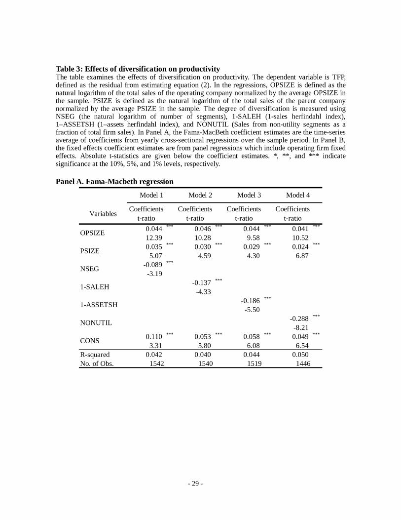
Table 3 examines the impact of diversification on productivity using the specification in Equation

(4). Panel A shows cross-sectional effects of diversification on TFP, where the regressions are

estimated using Fama-Macbeth regressions. These estimations examine how the diversification

measures affect firms’ TFP at a given point in time, only making use of the cross-sectional variation in

the data. Model 1 uses the logarithm of number of segments as a diversification measure, Model 2 uses

(1 - sales herfindahl), Model 3 uses (1 - assets herfindahl), and Model 4 uses the ratio of revenue from

non-utility businesses to the total revenue of the parent company. All models show that diversified

parents have less productive utility businesses. The coefficients on the diversification measures are all

negative and significant at the 1% level. Also, the results are economically significant, a one standard

deviation increase in (1-sale herfindahl) leads to a 3% drop in productivity. This result is consistent

with the literature that there exists a diversification discount. Using plant-level data from the U.S.

Census Bureau, Maksimovic and Phillips (2002) also find that conglomerate firms are less productive

than single-segment firms.

Insert Table 3 around here.

However, it is unclear from such cross-sectional regressions whether the negative coefficients on

the diversification variables are due to the fact that diversification reduces productivity or whether

parents with less productive operating companies choose to diversify. Papers such as Campa and Kedia

(2002) and Villalonga (2004) argue that the conglomerate discount arises endogenously. Consistent

with this argument, Jandik and Makhija (2005) find that underperforming electric utilities are more

likely to diversify. The model in Maksimovic and Phillips (2002) shows that the reduced productivity

of conglomerate firms relative to single-segment firms can be consistent with profit-maximization. In

- 17 -

their model, firms have differential comparative advantage across different industries. Therefore, firms

which are relatively more productive in a specific industry have higher opportunity costs of diversifying

and thus, in equilibrium, single-segment firms have higher productivity than conglomerates. In their

model, it may be optimal for a firm which is relatively less efficient in a specific industry to diversify

into other industries. Thus, it is possible that the time-series dynamic relation between diversification

and productivity may be different compared to the cross-sectional relation. Therefore, we next examine

whether diversifying activities lead to a worsening of productivity at the operating company or not.

We estimate Equation (4) using fixed effects estimation in Panel B. By including operating firm

fixed effects, not only can we examine the temporal effects of diversification on productivity, we can

also control for any unobserved characteristics of the operating company that can affect the relation

between productivity and diversification. In contrast to the cross-sectional results in Panel A, the

results in Panel B indicate that increases in parent’s degree of diversification positively influence the

TFP of their operating companies.

Taken together, Table 3 shows that diversified parent companies have lower productivity in their

operating companies as compared to single-segment parent companies. However, diversification into

other non-utility-related segments in fact helps to increase the productivity of their utility segment.

Our results so far are different from the results in Schoar (2002), who finds that diversified firms

have higher productivity in the cross-section, but the act of diversification reduces productivity. Our

results are however consistent with Maksimovic and Phillips (2002) who find that diversified firms are

less productive than single-segment firms of similar size, except for the smallest firms. One reason for

the difference in results between Schoar (2002) and ours could be due to the differing conditions under

which firms in her sample and our sample undertake their diversifying activities. Jensen (1986) argues

that investments undertaken by cash-rich, low-growth firms are likely to be value-destroying.

Therefore, diversification activities may not always be efficiency-decreasing, the productivity effects

depend on whether the firms have excess resources for investments and whether there are good

investment opportunities available. Therefore, in subsequent sections, we examine whether

- 18 -

diversification undertaken when firms are financially constrained have a different impact on productivity

compared to when firms are not financially constrained. The impact of financial constraints on the

productivity and value effects of diversification has not been examined before.

4.2. Productivity, Diversification, and Financial Constraints

We first examine the impact of financial constraints on productivity. The specification we

estimate is:

( ) ( ) ( ) ( ) ,14321 ntntntntntnt KZbDivbPSizebOPSizebaTFP ε+++++= − (5.)

where 1−ntKZ is the KZ-index from Kaplan and Zingales (1997) and measures the degree of financial

constraints and financial slack the parent company faces. Higher values of the KZ-index indicate

higher financial constraints and lower slack.

Insert Table 4 around here.

Table 4 summarizes estimation results of Equation. (5). Panel A provides cross-sectional results

using Fama-MacBeth regressions, while Panel B shows the dynamic effects of financial constraints on

TFP using fixed effects estimations. The results show that financial constraints negatively affect TFP

both in the cross-section and in the time series. Companies faced with financial constraints likely do

not have enough resources to invest in profitable projects or new technology therefore resulting in lower

efficiency of the operating firms. In untabulated results, we measure financial constraints using interest

coverage and the results are generally robust to this alternative measure of financial constraints.

Controlling for the KZ-index in the regressions reduces the statistical significance of the

coefficients on the diversification variables. Importantly, the signs of the coefficients on the

diversification variables are similar to those in Table 3. In Panel A, diversification is again negatively

associated with productivity in the cross-section, although only the coefficient estimates on the logarithm

of number of segments and (1-asset herfindahl) is significant at conventional significance level. In

- 19 -

Panel B, the coefficient estimates on diversification are positive for all models. However, only the ratio

of non-utility sales to total sales is significant.

Table 4 does not allow us to determine the impact of financial constraints and financial slack on

the productivity effects of diversification. To examine whether diversification undertaken when the

firm is financially constrained has a different impact on productivity compared to diversification

undertaken when there is financial slack, we introduce interaction terms between the level of

diversification and the KZ-index. Specifically, we estimate the below specification:

( ) ( ) ( ) ( ) ( )( )( ) ( )( ) , 1817

1615321

ntntntntnt

ntntntntntnt

KZLDivbKZHDivb

KZLbKZHbDivbPSizebOPSizebaTFP

ε++++++++=

−−

−− (6.)

where KZH takes the value of one when the firm’s KZ-index belongs to the top tercile of KZ-index

values in the year, and zero otherwise. In contrast, KZL takes the value of one when the firm’s

KZ-index belongs to the bottom tercile of KZ-index values in the year, and zero otherwise. Since we

are interested in the dynamic effects of diversification on productivity, we estimate Equation (6) using

the fixed effects estimation.

In this study, we refer to firm-years where KZ-index is in the top tercile (KZH equals one) as

being financially constrained while firm-years where the KZ-index is in the bottom tercile (KZL equals

one) are considered as being financially unconstrained. It is important to note that we do not mean that

firms in the top tercile are completely constrained while firms in the bottom tercile are completely

unconstrained. This segregation of the firm-years based on their KZ-index merely implies that firms in

the top tercile are relatively more constrained than firms in the bottom tercile. Therefore, 7b

measures the impact of diversification on productivity for relatively more constrained firms while 8b

measures the impact of diversification on productivity for firms with relatively more financial slack.

Our hypothesis predicts that 7b will be greater than 8b , i.e., diversification undertaken during

financial slack has a negative impact on productivity compared to diversification undertaken when the

firm is relatively more constrained.

- 20 -

Insert Table 5 around here.

Table 5 summarizes the estimation results of Equation (6) obtained from fixed effects estimation.

First, all the diversification measures are positive and significant for all models. This is consistent with

the results in Panel B of Table 3. Second, the coefficient estimates of KZH are negative and those of

KZL are positive in all the models. The coefficients on KZH and KZL are all statistically significant at

conventional levels with the exception of KZH of Model 1. Consistent with results in Table 4, the

results show that severe financial constraints are associated with decreases in TFP, while moderate

financial constraints or financial slack is associated with increases in TFP. More interestingly, we find

that the negative impact of diversification on productivity is only among firms with financial slack.

The interaction term between KZL and the diversification variables are all negative and significant for

the first three models. There is no such negative impact of diversification on productivity for the

financially constrained firms. In fact, the coefficients on the interaction term between the

diversification variables and KZH are generally positive, although insignificant. We test for whether

the coefficient estimates on the interaction terms (i.e., 7b and 8b ) are significantly different from each

other. The F-statistics and the corresponding P-values are listed at the bottom of Table 5. All the

F-statistics reject the null hypothesis that the coefficient estimates are the same between cross-terms of

the diversification measure with KZH and that with KZL, further supporting the hypothesis that different

financial conditions have an impact on whether diversification activities are good or bad for the firm.

In untabulated results, we replicated Table 5 using interest coverage as an alternative measure of

financial constraint and the results are similar.

These results also reconcile Table 3 with results in Schoar (2002) who finds that diversification

activities lead to a negative impact on the productivity of incumbent plants. She argues that this is

because of the “new toy” effect. Managers who diversify shift their focus to the new segment,

therefore neglecting the incumbent segments. This neglect by management leads to reduction in the

- 21 -

productivity of the incumbent segments. In Table 5, we find that diversification undertaken when firms

have excess resources relative to investment opportunities leads to negative impact on the productivity

of the incumbent utility segment, but when firms are financially constrained, diversification in fact has a

positive effect on the productivity of the utility segment. Therefore, when considering the impact of

diversification on productivity, it is important to consider the financial conditions under which the

diversification activities are taken.

4.3. Robustness check

Fixed effects estimation makes use of the within-firm variation to derive the coefficient estimates,

thus including operating companies which do not experience any changes in diversification would

introduce noise into the estimation. As can be seen from Table 6, deleting operating companies which

do not experience any changes in diversification leads to stronger results. The absolute value of the

coefficients on the interaction term between diversification and KZL are slightly larger than those in

Table 5 and now the interaction term between the ratio of non-utility sales to total sales is significant at

the 10% level.

Insert Table 6 around here.

Even though we study a period during which diversification activities are not seriously regulated,

we allow for the possibility that there are other regulatory effects. In Table 7, we examine whether

deregulation efforts in the utility industry would affect our results. The year, 1996, is important from

the perspective of industrial policy for the electric utilities, because FERC issued Orders 888 and 889

that allowed market participants for accessing transmission lines to promote wholesale power trading

and foster competition in the industry. In addition, restructuring legislations on the electric utility

industry were passed in some states (e.g., Rhode Island and California) in 1996. Hence, we introduce

additional variables to control for effects of deregulation. Reg96 is a dummy variable that takes the

- 22 -

value of one during the period from 1996 to 2003, and zero otherwise. We also interact Reg96 with the

diversification variables. Again, the conclusion remains the same even after controlling for

deregulation. In particular, the deregulation variable and its cross-term with the diversification measure

are not statistically significant.

Insert Table 7 around here.

5. Conclusion

The electric utility industry provides for a natural setting to test for the impact of diversification

on productivity. Electric utilities produce a single homogenous product, which enables precise

measurement of productivity and comparison of productivity across firms. Also, the industry is large

enough with varying degrees of diversification across firms to viably test for the impact of

diversification on productivity. Using data from the period of deregulation, we find that operating

companies of diversified parent firms have lower productivity than those of focused parent firms in the

cross-section. However, in the time series, we find that productivity in the core utility segment

increases when the parent company diversifies. This increase in productivity is only among firms with

relatively high and moderate levels of financial constraints. When parent firms with financial slack

diversify, we find that the productivity of the operating company falls. This suggests that when

managers are faced with excess resources relative to their investment opportunities, they tend to invest in

“pet projects” which distracts them from their core business, leading to reductions in the productivity of

the electric utility operating company.

- 23 -

Appendix A: Construction of Capital Stock Data

This study constructs the capital stock data employing a perpetual inventory method. Capital

stock in current year t is defined as such:

( ) ,11t

ititit PI

GICSCS +−= − δ (A.1)

where itCS is the real-term capital stock for firm i in period t, itGI is the nominal-term gross capital

investments, and tPI is a price index for converting nominal terms to real terms. itGI is calculated

by summing up all gross additions to utility capital assets, obtained from the operating firm’s cash flow

statement. The depreciation rate,δ , is from the Bureau of Economic Analysis (BEA) at the U.S.

Department of Commerce, downloadable from http://bea.gov/bea/an/0597niw/tableA.htm. Specifically,

we use a constant depreciation rate of 0.0211 over the sample period, which is constructed for the

category of “private nonresidential structure－electric light and power.”

The capital stock for the base-year, i.e., 1990, is constructed by applying a “triangularized”

weighted average procedure proposed by Cowing et al. (1981):

,1990 ,20

1

20

1

=

⎭⎬⎫

⎩⎨⎧

⎟⎠

⎞⎜⎝

⎛=

∑ ∑= =

b

PIrr

BKCS

rr

r

ibib (A.2)

where BKib is the book value of capital assets for firm i in the base-year. 1PI to 20PI corresponds to

1971PI to 1990PI , respectively.

The price index, PI, used in Equations A.1 and A.2 is obtained from the Price Indexes for

Gross Domestic Product Table published by the BEA. Specifically, we apply the decomposed index

constructed for the category of “Gross private domestic investment -- Fixed investment -- Nonresidential

structures.” This index is downloadable from

http://www.bea.gov/national/nipaweb/TableView.asp?SelectedTable=4&FirstYear=2004&LastYear=

2006&Freq=Qtr.

- 24 -

References

Baker, Malcom, Jeremy C. Stein, and Jeffrey Wurgler, 2003, When Does the Market Matter? Stock

Prices and the Investment of Equity-Dependent Firms, The Quarterly Journal of Economics

118, 969-1005.

Berger, Philip G., and Eli Ofek, 1995, Diversification’s Effect on Firm Value, Journal of Financial

Economics 37, 39-65.

Campa, Jose Manuel, and Simi Kedia, 2002, Explaining the Diversification Discount, Journal of Finance

57, 1731-1762.

Comment, Robert, and Gregg A. Jarrell, 1995, Corporate Focus and Stock Returns, Journal of Financial

Economics 37, 67-87.

Denis, David J., Diane K. Denis, and Atulya Sarin, 1997, Agency Problems, Equity Ownership, and

Corporate Diversification, Journal of Finance 52, 135-160.

Fama, Eugene F., and James D. MacBeth, 1973, Risk, Return, and Equilibrium: Empirical Tests, Journal

of Political Economy 81, 607-636.

Graham, John R., Michael L. Lemmon, and Jack G. Wolf, 2002, Does Corporate Diversification Destroy

Value?, Journal of Finance 57, 695-720.

Harford, Jarrad, 1999, Corporate Cash Reserves and Acquisitions, Journal of Finance 54, 1969-97.

Jandik, Tomas, and Anil K. Makhija, 2005, Can Diversification Create Value? Evidence from the

Electric Utility Industry, Financial Management 34, 61-93.

Jensen, Michael C., 1986, Agency Costs of Free Cash Flow, Corporate Finance and Takeovers, American

Economic Review 76, 323-329.

Jensen, Michael C., 1993, The Modern Industrial Revolution, Exit, and the Failure of Internal Control

Systems, Journal of Finance 48, 831-880.

Jensen, Michael C., and William H. Meckling, 1976, Theory of the Firm: Managerial Behavior, Agency

Costs, and Ownership Structure, Journal of Financial Economics 3, 305-360.

- 25 -

Joskow, P. (2000), “Deregulation and Regulatory Reform in the US Electric Power Sector,” in

Deregulation of Network Industries: What’s Next? ed. Sam Peltzman and Clifford Winston,

113-188. Washington, D.C.: AEI-Brookings Joint Center for Regulatory Studies, Brookings

Institution Press.

Kaplan, Steven N., and Luigi Zingales, 1997, Do Investment-Cash Flow Sensitivities Provide Useful

Measures of Financing Constraints?, Quarterly Journal of Economics 112, 169-215.

Lamont, Owen, Christopher Polk, and Jesus Saa-Requejo, 2001, Financial Constraints and Stock Returns,

Review of Financial Studies 14, 529-554.

Lang, Larry H. P., and René M. Stulz, 1994, Tobin’s Q, Corporate Diversification and Firm Performance,

Journal of Political Economy 102, 1248-1280.

Lang, Larry H. P., Rene M. Stulz, and Ralph A. Walkling, 1991, A Test of the Free Cash Flow

Hypothesis: The Case of Bidder Returns, Journal of Financial Economics 29, 315-35.

Lins, K. V., and H. Servaes, 2002, Is Corporate Diversification Beneficial in Emerging Markets?,

Financial Management 31, 5-31.

Lins, Karl, and Henri Servaes, 1999, International Evidence on the Value of Corporate Diversification,

Journal of Finance 54, 2215-2239.

Maksimovic, Vojislav, and Gordon Phillips, 2001, The Market for Corporate Assets: Who Engages in

Mergers and Asset Sales and Are There Efficiency Gains? Journal of Finance 56, 2019-65.

Maksimovic, Vojislav, and Gordon Phillips, 2002, Do Conglomerate Firms Allocate Resources

Inefficiently across Industries? Theory and Evidence, Journal of Finance 57, 721-767.

Malmendier, Ulrike M., and Geoffrey Tate, 2005, CEO Overconfidence and Corporate Investment,

Journal of Finance 60, 2661-2700.

Morck, Randall, Andrei Shleifer, and Robert W. Vishny, 1990, Do Managerial Objectives Drive Bad

Acquisitions?, Journal of Finance 45, 31-48.

Schoar, Antoinette, 2002, Effects of Corporate Diversification on Productivity, Journal of Finance 57,

2379-2403.

- 26 -

Servaes, Henri, 1996, The Value of Diversification During the Conglomerate Merger Wave, Journal of

Finance 51, 1201-1225.

Sing, M. (1987), “Are Combination Gas and Electric Utilities Multiproduct Natural Monopolies?”

Review of Economics and Statistics, 69 (3), 392-398.

Stein, Jeremy C., 2003, Agency, Information and Corporate Investment, Handbook of the economics of

finance. Volume 1A. Corporate finance (Elsevier, North Holland, Amsterdam; London and

New York).

Villalonga, Belen, 2004, Does Diversification Cause the 'Diversification Discount'?, Financial

Management 33, 5-27.

- 27 -

Table 1: List of sample firms The table lists the investor-owned electric power utilities (IOUs) and their parent firms in our sample. IOUs corresponding to more than one parent changed ownership during the sample period. Parent firms are identified using information from company websites and 10-K filings. Changes in ownership of the IOUs are also obtained from SDC’s Mergers and Acquisitions database.

Number Company Name Parent Company STATENumber Company Name Parent Company STATE Number Company Name Parent Company STATE

1 AEP Texas Central Co. Central and South West Corporation OH 39 Edison Sault Electric Co. ESELCO Inc MI 84 PacifiCorp PACIFICORP ORAmerican Electric Power Co., Inc. Wisconsin Energy Corp. 85 PECO Energy Co. Exelon Corp. PA

2 AEP Texas North Co. Central and South West Corporation OH 40 El Paso Electric Co. El Paso Electric Co. TX 86 Pennsylvania Electric Co. GPU Inc OHAmerican Electric Power Co., Inc. 41 Electric Energy, Inc. Ameren Corp. IL FirstEnergy Corp.

3 Alabama Power Co. Southern Co. AL 42 Empire District Electric Co. Empire District Electric Co. MO 87 Pennsylvania Power Co. FirstEnergy Corp. OH4 Alaska Electric Light & Power Co. AK 43 Entergy Arkansas, Inc. Entergy Corp. AR 88 Potomac Edison Co. Allegheny Energy, Inc. PA5 Appalachian Power Co. American Electric Power Co., Inc. OH 44 Entergy Gulf States, Inc. Entergy Corp. TX 89 Potomac Electric Power Co. PEPCO Holdings, Inc. DC6 Aquila Inc. Aquila, Inc MO 45 Entergy Louisiana, Inc. Entergy Corp. LA 90 PPL Electric Utilities Corp. PPL Corp. PA7 Arizona Public Service Co. Pinnacle West Capital Corp. AZ 46 Entergy Mississippi, Inc. Entergy Corp. MS 91 PSC of Colorado NEW CENTURY ENERGIES INC CO8 Atlantic City Electric Co. Atlantic Energy Inc NJ 47 Entergy New Orleans, Inc. Entergy Corp. LA Xcel Energy, Inc.

Conectiv 48 Fitchburg Gas & Electric Light Co. Fitchburg Gas & Electric Lt.Co. MA 92 PSC of New Hampshire PUBLIC SERVICE CO OF NH NHPEPCO Holdings, Inc. Unitil Corp. Northeast Utilities

9 Avista Corp. Avista Corp. WA 49 Florida Power & Light Co. FPL Group, Inc. FL 93 PSC of Oklahoma Central and South West Corporation OH10 Baltimore Gas & Electric Co. Constellation Energy Group, Inc. MD 50 Florida Power Corp. Florida Progress Corporation FL American Electric Power Co., Inc11 Bangor Hydro-Electric Co. BANGOR HYDRO ELECTRIC CO ME Progress Energy, Inc. 94 Public Service Co. of New Mexico PNM Resources NM12 Black Hills Power Inc. Black Hills Corp. SD 51 Georgia Power Co. Southern Co. GA 95 Public Service Electric and Gas Co. Public Service Enterprise Group, Inc. NJ13 Boston Edison Co. NSTAR MA 52 Green Mountain Power Corp. Green Mountain Power Corp. VT 96 Puget Sound Energy, Inc. Puget Energy, Inc. WA14 Cambridge Electric Light Co. Commonwealth Energy System MA 53 Gulf Power Co. Southern Co. FL 97 Rochester Gas & Electric Corp. R G S ENERGY GROUP INC NY

NSTAR 54 Hawaiian Electric Co., Inc. Hawaiian Electric Industries, Inc. HI Energy East Corp.15 Carolina Power & Light Co. Progress Energy, Inc. NC 55 Idaho Power Co. IDACORP, Inc. ID 98 Rockland Electric Co. ORANGE & ROCKLAND UTILS INC NY16 CenterPoint Energy Houston Electric, LLCCenterPoint Energy Inc. TX 56 Illinois Power Co. ILLINOVA CORP IL Consolidated Edison, Inc.17 Central Hudson Gas & Electric Corp. CH Energy Group, Inc. NY Dynergy Inc 99 San Diego Gas & Electric Co. ENOVA CORP CA18 Central Illinois Light Co. CILCORP Inc IL 57 Indiana Michigan Power Co. American Electric Power Co., Inc. OH Sempra Energy

AES Corp. 58 Indianapolis Power & Light Co. IPALCO Enterprises Inc. IN 100 Savannah Electric & Power Co. Southern Co. GAAmeren Corp. AES Corp. 101 Sierra Pacific Power Co. Sierra Pacific Resources NV

19 Central Illinois Public Services Co. C I P S C O INC IL 59 Kansas City Power & Light Co. Great Plains Energy Corp. MO 102 South Beloit Water, Gas & Electric CoAlliant Energy Corp. WIAmeren Corp. 60 Kentucky Power Co. American Electric Power Co., Inc. OH 103 South Carolina Electric & Gas Co. SCANA Corp. SC

20 Central Maine Power Co. C M P GROUP INC ME 61 Kentucky Utilities Co. KU Energy KY 104 Southern California Edison Co. Edison International CAEnergy East Corp. LG&E Energy 105 Southern Indiana Gas & Electric Co. SIGCORP Inc IN

21 Central Vermont Public Service Corp. Central Vermont Public Service Corp VT 62 KGE, A Westar Energy Co. Kansas Gas & Electric Co. KS Vectren Corp.22 Cincinnati Gas & Electric Co. Cinergy Corp. OH Westar Energy Inc. 106 Southwestern Electric Power Co. Central and South West Corporation OH23 Clark Fork & Blackfoot, LLC Montana Power Co MT 63 Kingsport Power Co. American Electric Power Co., Inc. TN American Electric Power Co., Inc

NorthWestern Corp. 64 Louisville Gas & Electric Co. LG&E Energy KY 107 Southwestern Public Service Co. SOUTHWESTERN PUBLIC SERVICE TX24 Cleco Power LLC Cleco Corp. LA 65 Madison Gas & Electric Co. MGE Energy Inc. WI NEW CENTURY ENERGIES INC25 Cleveland Electric Illuminating Co. Centerior Energy OH 66 Maui Electric Co., Ltd. Hawaiian Electric Industries, Inc. HI Xcel Energy, Inc.

FirstEnergy Corp. 67 Minnesota Power, Inc. ALLETE MN 108 Superior Water, Light & Power Co. ALLETE WI26 Columbus Southern Power Co. American Electric Power Co., Inc. OH 68 Mississippi Power Co. Southern Co. MS 109 Tampa Electric Co. TECO Energy, Inc. FL27 Commonwealth Edison Co. UNICOM CORP HOLDING CO IL 69 Monongahela Power Co. Allegheny Energy, Inc. WV 110 Texas-New Mexico Power Co. TNP ENTERPRISES INC TX

Exelon Corp. 70 Montana Dakota Utilities Co. MDU Resources Group, Inc. ND 111 Toledo Edison Co. Centerior Energy OH28 Commonwealth Electric Co. Commonwealth Energy System MA 71 Mount Carmel Public Utility Co. IL FirstEnergy Corp.

NSTAR 72 Nevada Power Co. Sierra Pacific Resources NV 112 Tucson Electric Power Co UniSource Energy Corp. AZ29 Connecticut Light & Power Co. Northeast Utilities CT 73 New York State Electric & Gas Corp. Energy East Corp. NY 113 Union Electric Co. Ameren Corp. MO30 Connecticut Valley Electric Co., Inc. Central Vermont Public Service Corp CT 74 Northern Indiana Public Service Co. NiSource Inc IN 114 Union Light, Heat & Power Co. Cinergy Corp. KY31 Consolidated Edison Co. Of New York IncConsolidated Edison, Inc. NY 75 Northern States Power Co. Xcel Energy, Inc. MN 115 United Illuminating Co. UIL Holdings Corp. CT32 Consumers Energy Co. CMS Energy Corp. MI 76 Northern States Power Co. Wisconsin Xcel Energy, Inc. WI 116 Upper Peninsula Power Co. UPPER PENINSULA ENERGY CORP MI33 Dayton Power & Light Co. DPL, Inc. OH 77

NorthWestern Energy,a Division of Northwestern Co

NorthWestern Corp. SD WPS Resources Corp.34 Delmarva Power & Light Co. Conectiv DE 78 Ohio Edison Co. FirstEnergy Corp. OH 117 Virginia Electric & Power Co. Dominion Resources, Inc. VA

PEPCO Holdings, Inc. 79 Ohio Power Co. American Electric Power Co., Inc. OH 118 West Penn Power Co. Allegheny Energy, Inc. PA35 Detroit Edison Co. DTE Energy Co. MI 80 Oklahoma Gas & Electric Co. (OG&EOGE Energy Corp. OK 119 Westar Energy Westar Energy Inc. KS36 Duke Energy Indiana, Inc. PSI Resources Inc IN 81 Orange & Rockland Utilities, Inc. ORANGE & ROCKLAND UTILS INC NY 120 Western Massachusetts Electric Co. Northeast Utilities MA

Cinergy Corp. Consolidated Edison, Inc. 121 Wheeling Power Co. American Electric Power Co., Inc. OH37 Duke Power Co. Duke Energy Corp. NC 82 Otter Tail Power Co. Otter Tail Corp. ND 122 Wisconsin Electric Power Co. Wisconsin Energy Corp. WI38 Duquesne Light Co. Duquesne Light Holdings, Inc. PA 83 Pacific Gas and Electric Co. PG&E Corp CA 123 Wisconsin Power & Light Co. Alliant Energy Corp. WI

124 Wisconsin Public Service Corp. WPS Resources Corp. WI

- 28 -

Table 2: Descriptive statistics The table provides the average, median, maximum, minimum, and standard deviation of the variables used. Panel A provides statistics of the variables used to estimate total factor productivity (TFP). Output is measured using total volume of electricity sold to final customers measured in Mega Watt hours. The two input variables are electric operation and maintenance (O&M) cost and capital stock. TFP is defined by the residuals from estimating Equation (2). The residuals indicate a percentage deviation of that firm’s TFP from the mean TFP of all firms in total samples. By this definition, the average TFP is close to 0. Panel B gives the statistics of variables describing the IOU and the parent company. OPSIZE (PSIZE) is the 3-year moving average of total sales of the IOU (parent company) in million dollars. All dollar values are in 2002 dollars. Segment data and accounting data for the parent company are from Compustat. The degree of diversification is measured using NSEG (number of segments), 1-SALEH (1-sales herfindahl index), 1–ASSETSH (1–assets herfindahl index), and NONUTIL (Sales from non-utility segments as a fraction of total firm sales). Financial constraints is measured using the Kaplan and Zingales (KZ) index, defined as

Panel A. Data for estimating TFP

Electricity Sales(1,000 MWh)

O&M Cost(Mio. $)

Capital Stock(Mio. $)

TFP (%)

Avg. 21,014 876.838 48.917 -1.217E-09

Med. 13,916 533.337 28.174 0.029

Max. 182,194 8,674.834 417.972 3.088

Min. 143 2.955 0.080 -2.867

S.D. 22,163 997.329 61.239 0.499

Panel B. Data for size, diversification, and financial constraints

OPSIZE PSIZE NSEG 1-SALEH 1-ASSETSH NONUTIL KZ

Avg. 1,354 3,838 2.653 0.268 0.262 0.161 0.227

Med. 822 2,425 3.000 0.287 0.241 0.092 0.136

Max. 8,425 41,330 9.000 0.789 0.820 0.962 4.041

Min. 9 29 1.000 0.000 0.000 -0.005 -3.478

S.D. 1,550 4,814 1.534 0.238 0.238 0.200 0.775

PPE

Cash

PPE

DividendsLeverageQ

PPE

CFKZ *1.315*39.368 *3.139*0.283*1.002 −−++−=

- 29 -

Table 3: Effects of diversification on productivity The table examines the effects of diversification on productivity. The dependent variable is TFP, defined as the residual from estimating equation (2). In the regressions, OPSIZE is defined as the natural logarithm of the total sales of the operating company normalized by the average OPSIZE in the sample. PSIZE is defined as the natural logarithm of the total sales of the parent company normalized by the average PSIZE in the sample. The degree of diversification is measured using NSEG (the natural logarithm of number of segments), 1-SALEH (1-sales herfindahl index), 1–ASSETSH (1–assets herfindahl index), and NONUTIL (Sales from non-utility segments as a fraction of total firm sales). In Panel A, the Fama-MacBeth coefficient estimates are the time-series average of coefficients from yearly cross-sectional regressions over the sample period. In Panel B, the fixed effects coefficient estimates are from panel regressions which include operating firm fixed effects. Absolute t-statistics are given below the coefficient estimates. *, **, and *** indicate significance at the 10%, 5%, and 1% levels, respectively. Panel A. Fama-Macbeth regression

VariablesCoefficients

t-ratioCoefficients

t-ratioCoefficients

t-ratioCoefficients

t-ratio

0.044 *** 0.046 *** 0.044 *** 0.041 ***

12.39 10.28 9.58 10.520.035 *** 0.030 *** 0.029 *** 0.024 ***

5.07 4.59 4.30 6.87-0.089 ***

-3.19-0.137 ***

-4.33-0.186 ***

-5.50-0.288 ***

-8.210.110 *** 0.053 *** 0.058 *** 0.049 ***

3.31 5.80 6.08 6.54R-squared 0.042 0.040 0.044 0.050No. of Obs. 1542 1540 1519 1446

Model 1 Model 2 Model 3 Model 4

OPSIZE

PSIZE

NSEG

1-SALEH

1-ASSETSH

NONUTIL

CONS

- 30 -

Panel B. Fixed effects estimation

VariablesCoefficients

t-ratioCoefficients

t-ratioCoefficients

t-ratioCoefficients

t-ratio

0.053 * 0.060 ** 0.051 * 0.067 **

1.78 2.04 1.69 2.26-0.031 *** -0.029 *** -0.034 *** -0.036 ***

3.86 3.77 4.21 -4.850.027 ***

3.290.077 ***

3.390.087 ***

3.820.055 *

1.74Adj. R-squared 0.914 0.914 0.915 0.933No. of Obs. 1542 1540 1519 1446

Model 1 Model 2 Model 3 Model 4

OPSIZE

NONUTIL

PSIZE

NSEG

1-SALEH

1-ASSETSH

- 31 -

Table 4: Effects of diversification and financial constraints on productivity The table examines the effects of diversification and financial constraints on productivity. The dependent variable is TFP, defined as the residual from estimating equation (2). In the regressions, OPSIZE is defined as the natural logarithm of the total sales of the operating company normalized by the average OPSIZE in the sample. PSIZE is defined as the natural logarithm of the total sales of the parent company normalized by the average PSIZE in the sample. The degree of diversification is measured using NSEG (the natural logarithm of number of segments), 1-SALEH (1-sales herfindahl index), 1–ASSETSH (1–assets herfindahl index), and NONUTIL (Sales from non-utility segments as a fraction of total firm sales). Financial constraints is measured using the Kaplan and Zingales (KZ) index. In Panel A, the Fama-MacBeth coefficient estimates are the time-series average of coefficients from yearly cross-sectional regressions over the sample period. In Panel B, the fixed effects coefficient estimates are from panel regressions which include operating firm fixed effects. Absolute t-statistics are given below the coefficient estimates. *, **, and *** indicate significance at the 10%, 5%, and 1% levels, respectively. Panel A. Fama-Macbeth regression

VariablesCoefficients

t-ratioCoefficients

t-ratioCoefficients

t-ratioCoefficients

t-ratioCoefficients

t-ratio

0.026 *** 0.030 *** 0.031 *** 0.030 *** 0.032 ***

5.33 5.62 5.56 5.52 5.250.037 *** 0.030 *** 0.024 ** 0.027 *** 0.021 ***

4.90 4.07 2.97 3.93 4.74-0.068 ***

-3.02-0.031

-0.66-0.107 **

-2.30-0.036-0.49

-0.080 *** -0.093 *** -0.085 *** -0.093 *** -0.094 ***

-4.86 -5.57 -5.10 -5.72 -6.020.040 *** 0.103 *** 0.037 * 0.057 *** 0.033 *

4.94 3.71 2.12 4.56 1.78R-squared 0.052 0.052 0.053 0.056 0.060No. of Obs. 1513 1434 1432 1411 1343

1-ASSETSH

NONUTIL

KZ

CONS

OPSIZE

PSIZE

NSEG

1-SALEH

Model 5Model 1 Model 2 Model 3 Model 4

- 32 -

Panel B. Fixed effects estimation

VariablesCoefficients

t-ratioCoefficients

t-ratioCoefficients

t-ratioCoefficients

t-ratioCoefficients

t-ratio

0.097 *** 0.085 *** 0.086 *** 0.090 *** 0.098 ***

3.18 2.90 2.96 2.98 3.07-0.001 0.003 0.004 0.007 -0.021 ***

-0.13 0.36 0.46 0.83 -2.660.012

1.610.035

1.610.016

0.720.065 **

1.96-0.009 -0.016 ** -0.016 ** -0.021 *** -0.024 ***

-1.31 -2.54 -2.53 -3.08 -3.71Adj. R-squared 0.885 0.902 0.902 0.902 0.916No. of Obs. 1513 1434 1432 1411 1343

1-ASSETSH

NONUTIL

KZ

OPSIZE

PSIZE

NSEG

1-SALEH

Model 1 Model 2 Model 3 Model 4 Model 5

- 33 -

Table 5: Impact of financial constraints on relation between diversification and productivity The table examines whether financial constraints affect the relation between diversification and productivity using the fixed effects estimation. The dependent variable is TFP, defined as the residual from estimating equation (2). KZH (KZL) is a dummy variable that takes 1 when the firm’s KZ index belongs to the top (bottom) 1/3 of the variable for each year and 0 otherwise. The other variables are as defined in the legend of Table 2. All models include operating firm fixed effects. Absolute t-statistics are given below the coefficient estimates. *, **, and *** indicate significance at the 10%, 5%, and 1% levels, respectively.

VariablesCoefficients

t-ratioCoefficients

t-ratioCoefficients

t-ratioCoefficients

t-ratio0.075 *** 0.075 *** 0.076 ** 0.095 ***

2.58 2.58 2.55 3.000.003 0.003 0.004 -0.025 ***

0.40 0.34 0.50 -3.130.028 **

2.500.076 **

2.450.052 *

1.710.096 **

2.01-0.023 -0.029 ** -0.035 ** -0.027 **

-1.58 -2.14 -2.53 -2.260.059 *** 0.060 *** 0.057 *** 0.025 *

3.78 4.03 3.92 1.93-0.003-0.18

-0.064 ***

-4.390.018

0.45-0.191 ***

-4.770.021

0.54-0.185 ***

-4.580.027

0.46-0.073

-1.39F statistics 15.94 23.43 22.10 3.23P value 0.000 0.000 0.000 0.073Adj. R-squared 0.904 0.904 0.905 0.916No. of Obs. 1434 1432 1411 1343

NONUTIL*KZL

SALEH*KZL

ASSETSH*KZH

ASSETSH*KZL

NONUTIL*KZH

KZL

NSEG*KZH

NSEG*KZL

SALEH*KZH

1-ASSETSH

NONUTIL

KZH

OPSIZE

PSIZE

NSEG

1-SALEH

Model 1 Model 2 Model 3 Model 4

- 34 -

Table 6: Robustness check: Sub-sample of parents which change diversification The table restricts the sample to parent firms which change their degree of diversification. The dependent variable is TFP, defined as the residual from estimating equation (2). KZH (KZL) is a dummy variable that takes 1 when the firm’s KZ index belongs to the top (bottom) 1/3 of the variable for each year and 0 otherwise. All models include operating firm fixed effects. Absolute t-statistics are given below the coefficient estimates. *, **, and *** indicate significance at the 10%, 5%, and 1% levels, respectively.

VariablesCoefficients

t-ratioCoefficients

t-ratioCoefficients

t-ratioCoefficients

t-ratio0.069 ** 0.069 ** 0.070 ** 0.092 ***

2.30 2.31 2.27 2.810.003 0.002 0.003 -0.025 ***

0.32 0.24 0.36 -3.150.030 ***

2.620.084 ***

2.610.061 *

1.930.102 **

2.07-0.025 * -0.032 ** -0.039 *** -0.029 **

-1.66 -2.27 -2.69 -2.250.072 *** 0.073 *** 0.070 *** 0.033 **

4.39 4.65 4.54 2.410.000-0.02

-0.073 ***

-4.810.0250.58

-0.217 ***

-5.220.0270.65

-0.210 ***

-5.030.0360.61

-0.090 *

-1.66F statistics 20.55 29.22 27.38 4.91P value 0.000 0.000 0.000 0.027Adj. R-squared 0.903 0.904 0.904 0.916No. of Obs. 1358 1356 1335 1269

Model 1 Model 2 Model 3 Model 4

OPSIZE

PSIZE

NSEG

1-SALEH

1-ASSETSH

NONUTIL

KZH

KZL

NSEG*KZH

NSEG*KZL

SALEH*KZH

NONUTIL*KZL

SALEH*KZL

ASSETSH*KZH

ASSETSH*KZL

NONUTIL*KZH

- 35 -

Table 7: Robustness check: Impact of regulation The table examines the impact of regulation. The dependent variable is TFP, defined as the residual from estimating equation (2). KZH (KZL) is a dummy variable that takes 1 when the firm’s KZ index belongs to the top (bottom) 1/3 of the variable for each year and 0 otherwise. Reg96 is a dummy variable that takes the value of 1 during the period from 1996 to 2003, and 0 otherwise. All models include operating firm fixed effects. Absolute t-statistics are given below the coefficient estimates. *, **, and *** indicate significance at the 10%, 5%, and 1% levels, respectively.

VariablesCoefficients

t-ratioCoefficients

t-ratioCoefficients

t-ratioCoefficients

t-ratio0.075 ** 0.073 ** 0.075 ** 0.092 ***

2.52 2.44 2.45 2.780.004 0.002 0.005 -0.026 ***

0.52 0.25 0.58 -3.150.037 ***

2.580.071 *

1.860.086 **

2.160.066

0.06-0.023 -0.029 ** -0.033 ** -0.027 **

-1.56 -2.14 -2.45 -2.240.059 *** 0.060 *** 0.057 *** 0.025 *

3.80 4.02 3.94 1.94-0.002

-0.16-0.064 ***

-4.380.018

0.45-0.191 ***

-4.770.022

0.56-0.185 ***

-4.580.021

0.37-0.077-1.45

0.009 0.002 0.012 -0.0020.90 0.16 1.29 -0.26

-0.014-1.15

0.0030.10

-0.051-1.53

0.037

0.94

F statistics 16.00 23.41 22.29 3.12

P value 0.000 0.000 0.000 0.078

Adj. R-squared 0.904 0.904 0.905 0.916

No. of Obs. 1434 1432 1411 1343

NONUTIL*KZL

(1-SALEH)*KZL

NONUTIL*KZH

(1-ASSETSH)*KZH

(1-ASSETSH)*KZL

(1-SALEH)*Reg96

(1-ASSETSH)*Reg96

Model 4

OPSIZE

PSIZE

NSEG

Model 2 Model 3

(1-SALEH)*KZH

NSEG*Reg96

NONUTIL*Reg96

Model 1

NONUTIL

KZH

Reg96

KZL

NSEG*KZH

NSEG*KZL

1-SALEH

1-ASSETSH