Diverse evidence, independent evidence,and Darwin’s arguments from anatomy

and biogeography

ByCasey Helgeson

A dissertation submitted in partial fulfillment ofthe requirements for the degree of

Doctor of Philosophy(Philosophy)

at theUNIVERSITY OF WISCONSIN–MADISON

2013

Date of final oral examination: 04/02/2013

The dissertation is approved by the following members of the Final Oral Committee:

Elliott Sober, Hans Reichenbach Professor & Vilas Research Professor, PhilosophyMalcolm Forster, Professor, PhilosophyMichael Titelbaum, Assistant Professor, PhilosophyPeter Vranas, Professor, PhilosophyDavid Baum, Professor, Botany

i

Contents

preface vi

1 introduction 1

I Darwin 5

2 Modus Darwin Reconsidered 62.1 Introduction . . . . . . . . . . . . . . . . . . . . . . . . . . . . . . . . 62.2 Modus Darwin . . . . . . . . . . . . . . . . . . . . . . . . . . . . . . 8

2.2.1 A single dichotomous character . . . . . . . . . . . . . . . . . 92.2.2 A single multistate character . . . . . . . . . . . . . . . . . . . 122.2.3 Overall similarity . . . . . . . . . . . . . . . . . . . . . . . . . 12

2.3 The correspondence problem . . . . . . . . . . . . . . . . . . . . . . . 132.3.1 Diagnosis . . . . . . . . . . . . . . . . . . . . . . . . . . . . . 182.3.2 From gene sequences to anatomy . . . . . . . . . . . . . . . . 20

2.4 First Conclusion . . . . . . . . . . . . . . . . . . . . . . . . . . . . . . 222.5 Geographical proximity . . . . . . . . . . . . . . . . . . . . . . . . . . 23

2.5.1 Proximity, ergo common ancestry . . . . . . . . . . . . . . . . 242.5.2 Criticism . . . . . . . . . . . . . . . . . . . . . . . . . . . . . . 27

2.6 Second Conclusion . . . . . . . . . . . . . . . . . . . . . . . . . . . . 32

3 Pattern as Observation 333.1 Introduction . . . . . . . . . . . . . . . . . . . . . . . . . . . . . . . . 333.2 Overview of chapters eleven and twelve . . . . . . . . . . . . . . . . . 413.3 The great facts: what, exactly, are the

relevant observations? . . . . . . . . . . . . . . . . . . . . . . . . . . 443.4 How the observations relate to theory . . . . . . . . . . . . . . . . . . 53

3.4.1 Darwin’s hypothesis . . . . . . . . . . . . . . . . . . . . . . . 54

ii

3.4.2 Were Darwin’s hypothesis correct . . . . . . . . . . . . . . . . 553.4.3 Objections . . . . . . . . . . . . . . . . . . . . . . . . . . . . . 603.4.4 Alternative hypotheses . . . . . . . . . . . . . . . . . . . . . . 62

3.5 Phylogenetic congruence . . . . . . . . . . . . . . . . . . . . . . . . . 653.6 Conclusion . . . . . . . . . . . . . . . . . . . . . . . . . . . . . . . . . 65

II Diversity 67

4 The Confirmational Significance of Agreeing Measurements 684.1 Introduction . . . . . . . . . . . . . . . . . . . . . . . . . . . . . . . . 684.2 Examples of the Phenomenon to be Analyzed . . . . . . . . . . . . . 704.3 Measurement Formally Characterized . . . . . . . . . . . . . . . . . . 724.4 Agreement as Observation . . . . . . . . . . . . . . . . . . . . . . . . 734.5 A Competing Super-model . . . . . . . . . . . . . . . . . . . . . . . . 774.6 Application . . . . . . . . . . . . . . . . . . . . . . . . . . . . . . . . 794.7 Evidential Diversity? . . . . . . . . . . . . . . . . . . . . . . . . . . . 824.8 Conclusion . . . . . . . . . . . . . . . . . . . . . . . . . . . . . . . . . 86

5 Evidential Diversity in Hierarchically Structured Hypothesis Spaces 885.1 Introduction . . . . . . . . . . . . . . . . . . . . . . . . . . . . . . . . 885.2 Formal Example . . . . . . . . . . . . . . . . . . . . . . . . . . . . . . 90

5.2.1 Setup . . . . . . . . . . . . . . . . . . . . . . . . . . . . . . . 905.2.2 Analysis . . . . . . . . . . . . . . . . . . . . . . . . . . . . . . 92

5.3 “Diversity” and “Kinds” . . . . . . . . . . . . . . . . . . . . . . . . . 995.4 Application . . . . . . . . . . . . . . . . . . . . . . . . . . . . . . . . 995.5 The Correlation Approach . . . . . . . . . . . . . . . . . . . . . . . . 101

5.5.1 My proposal and the correlation approach . . . . . . . . . . . 104

Wrap Up 112

Appendices 115

R code for probability calculations 116

iii

List of Tables

3.1 A representation of Darwin’s flightless birds and rodents examples.In each case, taxonomic relations are juxtaposed with groupings ac-cording to migratory accessibility, and environmental similarity of thecorresponding geographical regions. Bold text highlights the groupson which taxonomy and accessibility agree. Incomplete statementssuch as (abc)d should be read as disjunctions, consistent with any ar-rangement that respects the stated grouping(s), in this case ((ab)c)d,or (a(bc))d, or ((ac)b)d. . . . . . . . . . . . . . . . . . . . . . . . . . 50

3.2 Pairwise migratory accessibility (using cartoon numbers) arranged todisplay the formal identity with a matrix of pair-wise character ‘dis-tances’ as used by some methods of tree construction. The two rheasare the most accessible, while all other pairs are about equally (andmuch less) accessible. (For simplicity, I assume that migratory acces-sibility is symmetric.) . . . . . . . . . . . . . . . . . . . . . . . . . . . 57

5.1 Hypotheses 1–4 make different homogeneity assumptions. Hypothesis1 says that p(heads) is constant across all four data collection methods,whereas hypothesis 4 says that p(heads) may be (and probably is)different for each method. Hypotheses 2 and 3 are intermediate inhow much they partition the total data into parts inhomogeneouswith respect to p(heads). . . . . . . . . . . . . . . . . . . . . . . . . . 92

5.2 The table displays eight values for the expression that Wheeler (2009)calls the “focussed correlation” of the observations relative to a hy-pothesis: that of observation sets {a, b, c, d} and {a40, b40} relative tohypotheses 1–4. . . . . . . . . . . . . . . . . . . . . . . . . . . . . . . 108

iv

List of Figures

2.1 Schematic diagrams illustrating lineages postulated by the separateancestry (SA) and common ancestry (CA) hypotheses . . . . . . . . . 10

2.2 Values for the likelihood ratio p(obs.|CA)/p(obs.|SA) at different num-bers of time steps of discrete time evolution, assuming that each siteevolves independently, starting from a uniform distribution over thefour states, and with state-change probabilities p(i → j) = 0.01 fori 6= j (i.e., drift). The two plots show likelihood ratios for the ob-servation of DNA sequences matching at 25% of sites, and at 50% ofsites. . . . . . . . . . . . . . . . . . . . . . . . . . . . . . . . . . . . . 17

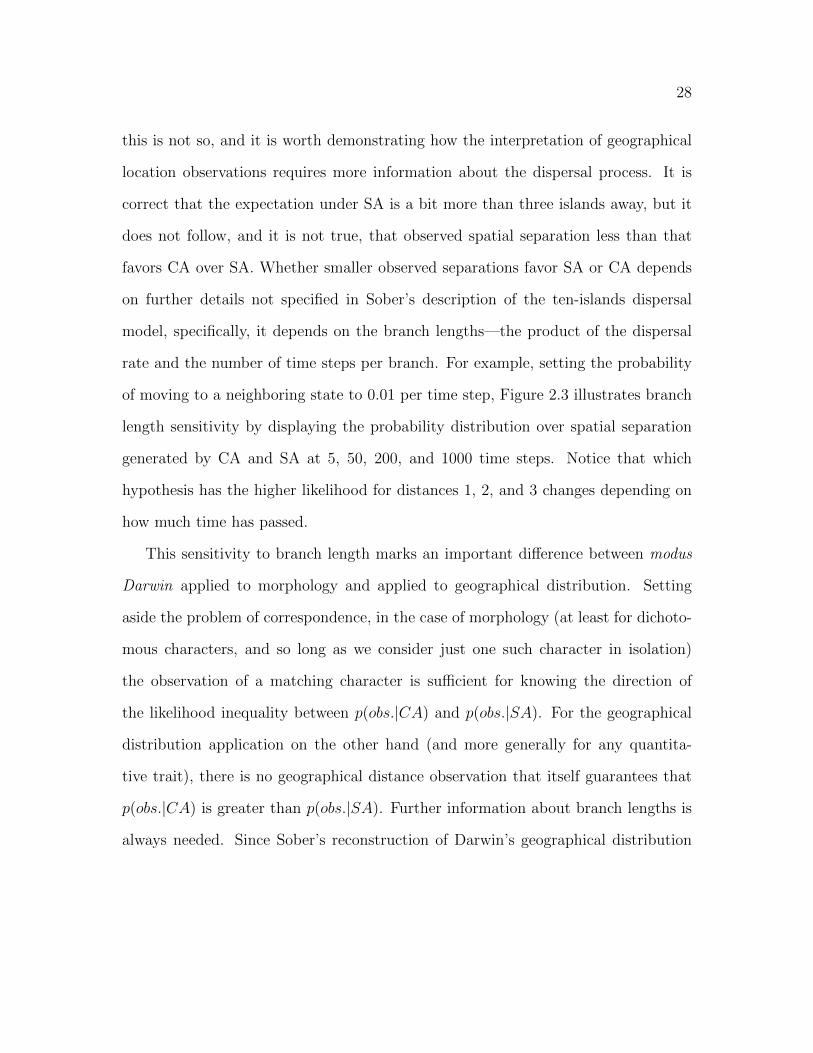
2.3 A series of probability distributions over spatial separation observedbetween species X and Y in Sober’s “ten-islands” dispersal model.All CA distributions assume µ = .01. The number of time steps (t)varies between plots. The SA distribution depends on neither µ nort, and is the same in every plot. . . . . . . . . . . . . . . . . . . . . . 29

2.4 Schematic representation of the relative distances between species{X1, . . . Xn, Y1, . . . Yn} where theXi inhabit the Galapagos archipelagoand the Yi inhabit the west coast of the South American mainland. . 31

3.1 As I interpret Darwin’s biota comparison language, biotas A and Bare more “similar” to each other than either is to biota C because thetaxonomic arrangement for species a, b, and c, drawn from their re-spective biotas using the rule described in the text, is typically (ab)c.Note that order from left to right carries no meaning; (ab)c is synony-mous with (ba)c, c(ba), and c(ab). . . . . . . . . . . . . . . . . . . . 48

v

3.2 A map showing the regions and species featured in Darwin’s flight-less birds example. The two rheas are closest taxonomic relations andinhabit the two regions with the greatest pair-wise mutual accessibil-ity. The ostrich and emu are the rheas’ closest taxonomic relationsfound in Africa and Australia respectively, but each is taxonomicallymore distantly related to the rheas than the rheas are to each other.The South America-Africa and South America-Australia environmentpairs are less accessible than the two South American regions are toone another. . . . . . . . . . . . . . . . . . . . . . . . . . . . . . . . . 50

3.3 An illustration of the one-to-one correspondence between groups-within-groups classificatory arrangements and (rooted) tree structures. . . . 56

4.1 Probability density distributions assigned to the agreement statisticby the one-parameter (solid line) and two-parameter (dashed line)super-models. (Distributions approximated via simulation.) . . . . . . 75

5.1 Two probability functions over possible values for the statistic |a− b|.The picture is exactly the same for the statistics |a− c|, and |a− d|.What changes from observation to observation is how many of thefour hypotheses are “equal thetas” versus “independent thetas” forthe relevant data collection methods. Likelihoods for each step ofBayesian conditionalization come from this plot (specifically, from thevalues at “difference in frequency” = 0.0, 0.05, and 0.1). . . . . . . . 95

5.2 Four probability distributions over hypoheses 1–4. Clockwise from theupper left, (1) a uniform prior distribution, (2) the posterior distribu-tion after conditionalizing on the observation that |a − b| = 0.1, (3)the posterior after subsequently conditionalizing on the observationthat |a−c| = 0.05, and (4) the final distribution after conditionalizingon the observation that |a− d| = 0. . . . . . . . . . . . . . . . . . . . 96

5.3 Probability distributions over hypotheses 1–4. The top row shows uni-form prior distributions (left) and posterior distributions after condi-tionalizing on four kinds of data (right). The bottom row shows uni-form prior distributions again (left) and posterior distributions afterconditionalizing on two kinds of data (right). The frequency differencestatistics are used as the observations for the darker bars, whereas thefrequencies themselves are the observations for the lighter colored bars.106

vi

preface

Among all the philosophy seminars in which I participated, two in particular had a

formative influence on my development as a philosopher, and on my thoughts about

my dissertation plan. Those seminars were “Evidence and Evolution” taught by

Elliott Sober, and “William Whewell” taught by Malcolm Forster. The plan that I

hatched in the wake of those seminars was basically to address a set of epistemolog-

ical problems in evolutionary biology by applying a Whewellian perspective on the

philosophy of science. I gathered a set of inference problems and illustrative scientific

arguments from evolutionary biology all of which seemed to turn on something like

Whewellian consilience; they included examples from Darwin’s Origin, contemporary

biogeography, phylogenetic inference, and contemporary arguments for the common

ancestry of all life. I hoped that studying these particular inference problems would

illuminate the epistemology of consilience, and vice versa.

As it happened, the first case study—Darwin’s geographical distribution argument—

proved difficult enough on its own, and I never got around to writing on the other

examples (as my prospectus committee predicted). In a second major development,

as I proceeded I found that writing on Darwin’s reasoning in particular, and also on

vii

consilience in general, required speaking to different target audiences. This pulled

the two sides of the project in somewhat different directions, resulting in the two-part

structure of this dissertation. The final product is less integrated than I had initially

imagined. It is a series of deeply interrelated essays, with some biggish gaps in be-

tween, and a lot of interesting loose ends. Not a book, it is more like one half of one

book, plus one half of another. Writing it has been a fabulous learning experience,

and has left me with more exciting research questions than I know what to do with.

Many people helped me through this learning process and deserve a lot of the

credit for whatever is good and valuable in this dissertation. The three (reading)

members of my committee deserve the most thanks. Elliott, my thesis advisor, has

provided constant feedback, advice, ideas, and encouragement since even before I

joined the graduate program. I have also worked very closely with Malcolm ever

since that Whewell seminar. What I’ve written in this dissertation owes very direct

intellectual debts to the work of both Elliott and Malcolm. I was very fortunate that

Mike Titelbaum joined our department along the way; his input and scrutiny has

been extremely helpful in framing and sharpening my ideas.

In addition to these three committee members, Dan Hausman participated in

my prospectus defense, and Peter Vranas will serve as the departmental non-reader

at my dissertation defense. Both have given substantive input at important points

along the way. David Baum (Botany) will serve as the non-departmental non-reader

at my defense. David taught or co-taught several seminars in the Botany department

in which I participated. In these seminars, David reliably cultivated the kind of en-

vironment where biologists and philosophers can productively communicate, and I

viii

owe much of what I’ve learned about interdisciplinary thinking and interdisciplinary

communication to my experiences in those seminars. Particularly relevant for my

dissertation was the iteration of Botany 940 (co-taught with Ken Cameron and Ken

Sytsma) in which we read Darwin’s Origin of Species. I’m thankful for that oppor-

tunity to go through the book with a mixed group of biologists and philosophers.

For additional feedback on various parts of this work, I thank Stephan Hartmann,

Jan Sprenger, Mary P. Winsor, Philip Kitcher, Jillian Scott McIntosh, Matt Barker,

Armin Schulz, Trevor Pearce, Lynn Nyhart, Marek Kwiatkowski, Michael Goldsby,

Reuben Stern, Bill Saucier, Marty Barrett, and all of the participants in the philos-

ophy department dissertators’ group, the philosophy of biology reading group, Lynn

Nyhart’s history and philosophy of biology reading group, and Malcolm Forster’s

graduate seminar “Case Studies in Philosophy of Science” (esp. Elena Spitzer, Josh

Mund, Emi Okayasu, Clinton G. Packman, and Brian McLoone).

In addition, I thank audiences at the UW Madison, the “Celebration of Darwin”

conference (Blacksburg, VA 2009), the Tilburg Center for Logic and Philosophy

of Science (Tilburg, Netherlands 2010), the Biennial Meeting of the International

Society for History, Philosophy, and Social Studies of Biology (Salt Lake City, Utah,

2010), the Biennial Meeting of the Philosophy of Science Association (San Diego,

California, 2012), Washington University in St. Louis (2012), the London School of

Economics and Political Science (2013), and the American Philosophical Association

Pacific Division Meeting (San Francisco, CA 2013).

Help also came in the form of money. A Graduate Research Fellowship from the

National Science Foundation (2007) changed my life. I wrote some of this work while

ix

a visiting fellow at the Tilburg Center for Logic and Philosophy of Science (2010).

A summer of my research was funded by the Philosophy department’s Marcus and

Blanche Singer Graduate Fellowship (2012). Travel to conferences to present parts

of this work, or to take part in relevant workshops came from the UW Graduate

School’s Vilas Travel Grant, the Holtz Center for Science and Technology Studies

Research Travel Grant, and two travel grants from the Center for Philosophy of

Science at the University of Pittsburgh.

My apologies to any individuals or organizations that I have inadvertently ne-

glected in these acknowledgments.

1

Chapter 1

Introduction

In science, as in everyday life, multiple pieces of evidence that are diverse in charac-

ter, or that arrive from different quarters, sometimes work together, pointing to the

same conclusion. We tend to find this particularly convincing. But is our intuitive

reaction correct? Does a notion of kinds of evidence, or of diversity in the character

of the evidence, really have a place in rational inductive inference, or is it only, so to

speak, the total quantity of evidence that matters? One label for the phenomenon

of multiple sources of evidence working together for greater effect is “consilience”.

In this dissertation, I investigate the epistemology of consilience from two directions:

first, by reconstructing the reasoning involved in an important scientific argument

from Darwin’s Origin that ostensibly appeals to consilience, and second, by attempt-

ing to formally model the epistemological value of consilience in probabilistic terms.

2

Darwin

Darwin’s Origin is a good place to start for several reasons. The importance of a

hypothesis being supported by different kinds of evidence is frequently emphasized

in the philosophical literature commenting on Darwin’s argument in the Origin,

and Whewell’s term “consilience” occurs frequently in that literature. Indeed, Dar-

win’s argument in the Origin is among the scientific arguments—if not the scientific

argument—most frequently discussed in connection with consilience. But the term

has become (at least in the Origin literature) a label for poorly understood theory-

observation relations rather than a tool for elucidation those relations.

For example, Thagard (1978), Recker (1987), and Waters (2003) apply Whewell’s

take on scientific methodology to the tasks of articulating the content of the theory

there presented, spelling out exactly how Darwin’s many supporting observations

relate to that theory, and illuminating the rhetorical structure of his argument. I

believe the conclusions of these investigations are correct as far as they go, but that

they remain superficial due to a vague and inadequate reformulation of Whewells key

term “consilience”. These analyses employ roughly the same definition, according to

which a hypothesis enjoys consilience to the degree that it “explains separate classes

of facts” (where the “explains” relation remains entirely unanalyzed).1

The prevalence of this slack formulation is understandable given that Whewell

1One might wonder whether Whewell influenced Darwin’s scientific methodology. After all,Whewell was both a personal acquaintance of Darwin and one of Britain’s highest authoritieson the methodology of science (along with John Herschel and John Stuart Mill). This question isdiscussed in Ghiselin (1969), Ruse (1975), Thagard (1977), and Hodge (1991). Despite the historicaland cultural proximity of Darwin to Whewell, I will bracket questions about influence, and aboutwhether Darwin knowingly perceived (or presented) his own methodology in Whewellian terms.

3

sometimes glosses his own view in such terms.2 Also, Whewell’s more rigorous presen-

tation of consilience is quantitative in a way that may appear to preclude application

to a scientific treatise such as the Origin, which does not contain a single mathemat-

ical formula. But defining consilience in terms of explanation leaves the former as

obscure as the latter, and in fact Whewell does not do so. (He does sometimes use

the term “explains” informally, as will I). The notion of “separate phenomena” or

“different kinds of facts” is also in need of clarification, in Whewell’s own writing

as well as in modern appropriations of his terminology. I will approach the topic of

consilience from a more rigorously Whewellian perspective, informed in particular

by the Whewell interpretation of Forster (1988, 2011).

The part of Darwin’s reasoning that I will examine is his biogeography argument

for common ancestry. Here Darwin argues that distinct species share common ances-

try (and that evolution must therefore have occurred) based on how species resemble

one another anatomically and how they are distributed geographically around the

globe. How do those two kinds of observation work together? In Chapter 3, I present

a new answer to this question. But first, in Chapter 2, I critically assess an alter-

native account of the same observations (Sober 1999, 2008, 2011) —an account that,

were it correct, would render my own superfluous.

2See Whewell (1858/1989a, 153, 159), and (1860/1989b, 331)

4

Diversity

Beyond Darwin’s Origin there is the broader question of what evidential diversity

is—what makes observations different kinds? —and why it matters to the episte-

mology of science. In Chapter 4, I address a special case of evidential diversity

and Whewellian consilience sometimes called the agreement of independent mea-

surements, that is instantiated, among many other places, in Darwin’s geographical

distribution argument. I analyze the epistemic import of such agreement from an

abstract, formal perspective using the framework of Likelihoodist epistemology. In

Chapter 5, I expand on the results of Chapter 4 to address the issue of evidential

diversity more generally, taking the extra step from likelihoodist to Bayesian episte-

mology, the common language of much literature on the subject.

Each of the four substantive chapters has its own, more detailed introduction

that motivates the concerns of that chapter more specifically and better identifies the

audience and literature to which that particular part of the dissertation is addressed.

5

Part I

Darwin

6

Chapter 2

Modus Darwin Reconsidered

2.1 Introduction

The common ancestry of all extant life on Earth is a central tenant of modern

evolutionary biology. In his book On the Origin of Species (henceforth “Origin”)

Darwin took a giant step towards establishing this fact. Of course Darwin could

address only the portion of life on Earth of which nineteenth-century naturalists

were aware, and he wavered on whether there was a single primordial species, or

some smallish number bigger than one (Darwin 1859/2003, 483–4). None the less,

Darwin argued forcefully that vast swaths of life trace back to a common ancestors;

indeed this was his main conclusion in Origin (Darwin 1859/2003, 6). While entirely

qualitative and remarkably under-articulated by today’s standards, his arguments

were enormously convincing to his contemporaries (Bowler 1989; Larson 2004).

In a series of publications, Elliott Sober (Sober 1999; Sober and Steel 2002; Sober

7

2008, 2011) has sought to clarify and formalize Darwin’s defense of common ancestry,

and to generalize Darwin’s reasoning to encompass contemporary thinking about

newer evidence for common ancestry. Sober’s project is thus part exegesis, part

epistemology: How does Darwin argue?, and How does that argument justify common

ancestry? In answer to the first question, Sober attributes to Darwin the following

argument form:

Similarity, ergo common ancestry. This form of argument occurs so often

in Darwin’s writings that it deserves to be called modus Darwin. The

finches in the Galapagos Islands are similar; hence, they descended from

a common ancestor. Human beings and monkeys are similar; hence, they

descended from a common ancestor. The examples are plentiful, not just

in Darwin’s thought, but in evolutionary reasoning down to the present.

(Sober 1999, 265)

To address the epistemological question, Sober sets out to formalize modus Darwin

with mathematical rigor, ultimately deriving the force of the argument form from

the Law of Likelihood (explained below).

In this essay I review and critique Sober’s analysis of Darwin’s reasoning. In the

first stage of my analysis, I bracket exegesis and concentrate instead on the epistemic

merits of the argument form modus Darwin as Sober understands it. I will argue

that modus Darwin cannot rationally support Darwin’s common ancestry hypothesis.

From this conclusion it follows that either Darwin’s reasoning was flawed (he gave

bad reasons for a true conclusion) or he did not employ modus Darwin as Sober

understands it.

8

I then move on to address Sober’s application of modus Darwin to Darwin’s

geographical distribution observations—a variant of the argument form that could

be summarized as: Proximity, ergo common ancestry. I find less to fault in this

argument form, thought of in the abstract, though I argue that it does not illuminate

Darwin’s reasoning in the Origin.

2.2 Modus Darwin

Sober derives the normative force of modus Darwin from the Law of Likelihood (Hack-

ing 1965; Royall 1997; Sober 2008), according to which an observation supports one

hypothesis over another whenever that observation is more to be expected supposing

the one hypothesis were true, compared with supposing the other hypothesis were

true. More formally, observation o favors hypothesis h1 over hypothesis h2 if and

only if p(o|h1) > p(o|h2). Mapping this framework onto Darwin’s reasoning requires

identifying an observation o, and two hypotheses h1 and h2.

Similarity between two species (or larger taxa) is the observation o. The hypoth-

esis h1 is common ancestry (CA), which says that the two species descended from

a single ancestor species. The alternative hypothesis h2 is separate ancestry (SA),

meaning that the two species’ lineages trace back to separate origin-of-life events.

These are, however, only the rough, qualitative statements of o, h1, and h2. To

evaluate the inequality p(o|h1) > p(o|h2) Sober must specify the observation more

rigorously, and then formally characterize the hypotheses as stochastic (chancy) pro-

cesses that can produce such outcomes with some probability.

9

Regarding the observation o, any two organisms are similar in some ways and

dissimilar in others. It seems there are infinitely many ways to measure similarity.

Which is the right yardstick? Sober defers talk of overall similarity to begin with

a simpler and more tractable observation: that two species share the same trait on

a single dichotomous character. A dichotomous character is one that has just two

possible states, for example an insect might have wings or lack them, or the edge

of a leaf might be smooth or serrated. Coding morphology in terms of dichotomous

characters typically masks more continuous underlying variation, but dichotomous

characters are adequate in many scientific contexts, and they provide a convenient

starting point for the formalization of modus Darwin.

2.2.1 A single dichotomous character

Letting o be the observation that two species share the same trait on a single dichoto-

mous character, does o favor CA over SA sensu the Law of Likelihood? To generate

the required conditional probabilities Sober repurposes the idealizations and math-

ematical framework of contemporary phylogenetic inference, as follows. Represent

the two species as categorical variables X and Y , each of which can take states

{0, 1}, standing for the two possible states of the dichotomous character. So o is

both species in the same state (either X = 0 & Y = 0, or X = 1 & Y = 1). Each

hypothesis is then characterized by a schematic genealogy for the two species, plus

a stochastic model describing how the character variable changes states as it moves

along a line in the genealogy (Figure 2.1).

The model of character-state evolution (applied in the same way to all solid

10

 

SA CA

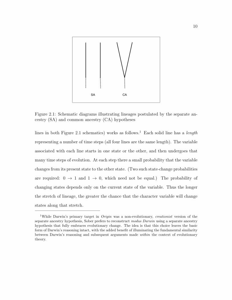
Figure 2.1: Schematic diagrams illustrating lineages postulated by the separate an-cestry (SA) and common ancestry (CA) hypotheses

lines in both Figure 2.1 schematics) works as follows.1 Each solid line has a length

representing a number of time steps (all four lines are the same length). The variable

associated with each line starts in one state or the other, and then undergoes that

many time steps of evolution. At each step there a small probability that the variable

changes from its present state to the other state. (Two such state-change probabilities

are required: 0 → 1 and 1 → 0, which need not be equal.) The probability of

changing states depends only on the current state of the variable. Thus the longer

the stretch of lineage, the greater the chance that the character variable will change

states along that stretch.

1While Darwin’s primary target in Origin was a non-evolutionary, creationist version of theseparate ancestry hypothesis, Sober prefers to reconstruct modus Darwin using a separate ancestryhypothesis that fully embraces evolutionary change. The idea is that this choice leaves the basicform of Darwin’s reasoning intact, with the added benefit of illuminating the fundamental similaritybetween Darwin’s reasoning and subsequent arguments made within the context of evolutionarytheory.

11

In which state does a variable begin? The starting state of a variable is determined

by a random draw from a probability distribution over the state space {0, 1}. The

difference between CA and SA is only that for SA, the beginning states of the two

variables are drawn independently from that distribution, whereas for CA just one

random draw is required because both lineages’ variables will begin in the same state

(think of this as the point just before speciation).

With CA and SA so characterized, Sober proves the following result: for X and

Y to end up in the same state at the end of the process is more probable on CA than

on SA regardless of lineage length, state-change probabilities, and the starting-state

distribution (Sober 2008, chap. 4).2 In other words, two species found in the same

state always favors CA over SA. It isn’t hard to understand intuitively why this is

so. If the state-change probabilities are small relative to the branch length, then the

most probable outcome along any branch is that a variable won’t change states at

all. In this case, since CA puts the two species in the same state at the start, chances

are good that they will both still be in the same state at the tips. The chances of

ending in the same state are somewhat smaller on SA, since X and Y may or may not

begin in the same state. As the probability of state change along a branch increases

(due either to long branch lengths or high state-change probabilities), p(o|CA) and

p(o|SA) converge to the same value, though p(o|CA) must always be a little bit

higher. The opposite is true for species found in different states: mismatches always

favor SA over CA.

2With these very minor assumptions: the starting-state distribution gives non-zero probabilitiesto both states, the transition probabilities are non-extreme (i.e., 6= 0 and 6= 1), and branch lengthsare finite.

12

2.2.2 A single multistate character

Sober generalizes the preceding treatment to also cover multistate characters, where

the variables X and Y can now take any number of states {1, 2, . . . n} and correspond-

ingly more state-change probabilities are needed: one for every possible transition

from one state to another (i → j, for all i, j ∈ {1, 2, . . . n}). Sober shows that, here

too, X and Y in the same state at the end of the process is more probable on CA

than on SA. Mismatches on multistate characters, however, are more complicated.

Some mismatches will still favor CA, while others will favor SA (depending on the

state-change probabilities).

2.2.3 Overall similarity

Next Sober aggregates many characters to arrive at something like overall similar-

ity. Given a whole set of observed characters—some matches and some mismatches,

which hypothesis is favored overall? Simply comparing the number of matches to

mismatches doesn’t answer the question. Some single-character observations favor

more strongly than others. In other words, the directions of the single-character

likelihood inequalities do not, on their own, provide enough information for aggre-

gating. Supposing that the process by which each trait evolves is probabilistically

independent of that governing every other trait,3 overall similarity favors CA over

SA if and only if the product of the likelihood ratios (one from each observed trait)

3While this assumption is certainly not true, it is a standard idealization in, e.g., phylogeneticinference from genetic data (thinking of each nucleotide site, or sometimes each codon, as a trait).

13

is greater than one, in mathematical notation:

m∏i=1

p(oi|CA)

p(oi|SA)> 1 (2.1)

where m is the number of individual traits observed. Calculating the individual

likelihood ratios p(oi|CA)/p(oi|SA) requires additional assumptions about the details

of the model of character evolution, in other words knowledge of the process by which

the trait evolved (whether by drift or selection, if by selection then how strong and

in what direction, and the time scale involved); see pp. 295–314, (Sober 2008) for

details.

2.3 The correspondence problem

Now for my criticism. I will argue that Sober’s characterization of the observations

themselves—the “similarity” in similarity, ergo common ancestry—illegitimately rigs

his likelihood comparison in favor of the common ancestry hypothesis. My argument

for this conclusion begins with an objection that Sober recognizes and discusses.

But I will argue that the objection is both more serious and more general than Sober

acknowledges.

Sober’s discussion of the modus Darwin inference form goes beyond Darwin’s own

thinking to encompass modern reasoning about data that Darwin lacked. Discussing

the application of modus Darwin to modern genetic sequence data, Sober identifies a

possible stumbling block. Let’s call it the correspondence problem. To appreciate the

worry, first think about how sequence data are used in phylogenetic inference. (Phy-

14

logenetic inference assumes common ancestry among a group of species and seeks

to discover the particular shape of their genealogical tree.) Sequence-based phyloge-

netic inference uses a small stretch of DNA from each species. But phylogeneticists

don’t simply draw a random sequence of DNA from each species. They use “corre-

sponding” sequences. In the final step of establishing sequence correspondence, two

DNA sequences are aligned, by sliding the one along the other and stopping when

the number of matching sites is greatest. But as Sober points out, this process seems

out of place in the context of modus Darwin:

At first glance, alignment seems not to make sense in this problem. Since

matching at a site is evidence for CA, aligning the sites so as to maxi-

mize matching seems to load the dice in favor of the common ancestry

hypothesis. But the problem is deeper. If two sequences have a common

ancestor, it makes sense to say that a site in one sequence “corresponds”

to a site in the other; this correspondence means that the two sites de-

rive from a site in their common ancestor. But if there was no such

common ancestor, what would alignment even mean? If we want to test

the separate-ancestry hypothesis rather than just assume from the outset

that it is false, we need to rethink the question of how sequence data can

be used. (Sober 2008, 291)

In response to this worry, Sober first points out that his modus Darwin likelihood

comparison can be carried out regardless of whether the sequences “correspond”.

Choose any sequence of length n from the genome of species A, and another from

15

that of species B. Treat the two sequences as states of a single character with 4n

possible states (four possible nucleotides for each site). Then:

By the argument given earlier, this matching counts as evidence of CA.

There is no need to align the sites to say this. The same point applies

when the sequences (each n sites long) drawn from the two species do

not match perfectly. They will then occupy different states of a single

character that has 4n possible states. Whether this difference between

the two species favors CA or SA depends on the rules of evolution that

govern how this complex character evolves. . . . The question is simply

whether the observed mismatch has a higher probability of arising under

the common-ancestry or the separate-ancestry hypothesis. To answer

this question, all that is needed is the two unaligned sequences and a

reasonable model for the process of sequence evolution. (Sober 2008,

291)

From this point about unaligned (i.e., non-corresponding) sequences, Sober draws

the following conclusion about aligned sequences:

An inference that begins with aligned sequences is valid to the extent that

it mimics the verdicts of the procedure that uses unaligned sequences.

When this is true, aligning sequences is not loading the dice. (Sober

2008, 291)

But this will not do. It is true that whether sequences are aligned makes no differ-

ence to the question; that question is always: Is the observation more probable on the

16

CA or SA hypothesis? The answer, however, does depend on whether sequences are

aligned. For this reason the verdict of the procedure that uses aligned sequences will

be systematically different from that of the procedure that uses unaligned sequences.

Some example calculations will illustrate.

Unaligned sequences will match at about one site in four. Is this more probable

on CA or SA? In the quotation above, Sober treats a DNA sequence as a single char-

acter with 4n possible states, but alternatively we can treat each site as one character,

where the resulting n likelihood ratios are aggregated as per Equation 2.1. I choose

the latter method here to simplify calculations. The probabilities p(obs.|CA) and

p(obs.|SA) depend on the details of the model of evolution, but for example, suppose

that all sites evolve independently by drift, with all four nucleotides equally probable

as starting states. Plot (a) in Figure 2.2 shows likelihood ratios p(o|CA)/p(o|SA)

with branch length increasing from left to right. That ratio is below 1 for all branch

lengths, meaning that matching at one in four sites always favors SA over CA.4 More-

over, one in four sites matching is typical of unaligned sites regardless of what species

are compared. Applying modus Darwin to unaligned sequences favors separate an-

cestry, not common ancestry. It doesn’t matter whether you compare a bacterium

with an elephant, or a human with her identical twin.

On the other hand, with the same assumptions about process, observing that two

sequences match at 50% of their sites favors common ancestry for all but extremely

4Note that Sober doesn’t describe overall similarity in terms of x%matching—he does notexplicitly use any measure of overall similarity (such as % of traits matching). Rather, whenconsidering the overall evidential weight of a set of traits, the observation is just the states ofeach species for each trait. In this particular case, however, the % of matching sites between thetwo DNA sequences is a sufficient statistic of that more complete description of the data, for thecalculation of the likelihood ratio p(o|CA)/p(o|SA).

17

0 10 20 30 40 50

0.0

0.2

0.4

0.6

0.8

1.0

(a) Likelihood ratios for 25% of sites matching

time steps

likel

ihoo

d ra

tio

0 10 20 30 40 50

0.0

0.5

1.0

1.5

(b) Likelihood ratios for 50% of sites matching

time steps

likel

ihoo

d ra

tio

Figure 2.2: Values for the likelihood ratio p(obs.|CA)/p(obs.|SA) at different num-bers of time steps of discrete time evolution, assuming that each site evolves in-dependently, starting from a uniform distribution over the four states, and withstate-change probabilities p(i→ j) = 0.01 for i 6= j (i.e., drift). The two plots showlikelihood ratios for the observation of DNA sequences matching at 25% of sites, andat 50% of sites.

18

short branch lengths (if branch lengths are short enough, then any mismatches at

all become extremely improbable on CA, since on that hypothesis all sites start off

matching; see plot (b) in Figure 2.2). Aligned DNA sequences match at far greater

than 50% of sites, so aligned sequences favor common ancestry on the assumption—

ubiquitous in the methodology of phylogenetic systematics—of sites evolving inde-

pendently by drift. Thus if the modus Darwin inference that begins with aligned

sequences is valid only to the extent that it mimics the verdicts of the procedure

that uses unaligned sequences, then it is not valid at all. Aligned sequences favor

CA, while unaligned sequences favor SA.

Thus, applying modus Darwin to genetic sequence data produces a dilemma.

Using aligned sequences loads the dice in favor of common ancestry—and the only

discernible justification for doing so begs the question by assuming CA. n the other

hand, using unaligned sequences favors separate ancestry, which is the wrong con-

clusion (wrong as in false, though not necessarily epistemically irrational).

2.3.1 Diagnosis

Applied fairly (i.e., to unaligned sequences), Sober’s Modus Darwin likelihood com-

parison systematically supports the wrong conclusion. What has gone wrong? The

problem is that the common-ancestry hypothesis that Sober intends to test via this

likelihood comparison is not the same as the hypothesis that actually appears in that

likelihood comparison. Sober’s qualitative statement of the the common-ancestry hy-

pothesis says only that the two species from which the sequences are drawn have a

common ancestor species, but if we’re going to take the likelihood comparison seri-

19

ously, we have to look more closely at the commitments of the precise, mathematical

description of CA. After all, it is that mathematical description that generates the

likelihood p(obs.|CA). That description goes beyond Sober’s informal statement

of CA; it says that the gene sequences themselves share a common gene sequence

ancestor, and that the two sequences are derived from that ancestor via a process

approximated by the stochastic model of character state evolution described above

(§§ 2.2.1–2.2.2). This is a very significant difference, because the sequence question

need not settle the species question. If two sequences do have a common ancestor

sequence, then (setting aside horizontal transfer) that means that the two species

from which the sequences were taken have a common ancestor species. But if the

two sequences do not have a common ancestor sequence (of the kind posited by the

mathematical description of CA) this leaves it entirely unsettled whether the species

have a common ancestor species.

For non-corresponding (unaligned) gene sequences, the sequence-CA hypothesis is

false, even if the two species from which the sequences are drawn do share a common

ancestor species. Sober intended for the modus Darwin likelihood comparison to

discriminate between SA and CA, the hypotheses that say, respectively, that species

A and species B do, and do not, have a common ancestor species. But what the

modus Darwin likelihood comparison in fact assesses is how the observation of two

sequences bears on the hypotheses that those particular sequences do or do not have

a common ancestor sequence. Thus, while applying modus Darwin to unaligned

sequences initially appeared to recommend the wrong answer, we can now see that

in fact it gives the right answer to a different question. A negative answer to this

20

new question does not settle the question Sober set out to ask.

2.3.2 From gene sequences to anatomy

The objection that I have been discussing so far—what I’m calling the problem of

correspondence—is one that Sober discusses while applying the modus Darwin argu-

ment form to modern genetic sequence data. So far I have argued that this problem

is more serious than Sober acknowledges. Indeed, it results in Sober’s likelihood com-

parison changing the subject. Rather than revealing what the evidence says about

CA versus SA, that likelihood comparison addresses a question about the history of

the particular DNA sequences compared. But it gets worse: now I argue that ex-

actly the same problem afflicts Sober’s reconstruction as applied to the anatomical

observations that Darwin used to argue for common ancestry. In other words, there

is nothing special about genetic sequence data; the correspondence problem is very

general.

Recall that Sober’s individual morphological similarities consist of two species

being in the same state for some single character. But each such observation implic-

itly treats the two characters as “the same” character seen in two different species.

Imagine comparing a spider with an insect. And consider, for example, the character:

number of appendages attached to the thorax. The insect has 6. What about the

spider? Before you can answer you must decide what counts as the spider’s thorax.

It’s the second of the insect’s three body sections, but the spider’s body has only two

sections; one section has zero appendages, the other has 10 (8 legs plus 2 chelicerae—

appendages by the mouth for grabbing food). So is the character state comparison

21

6 to 0?, 6 to 10?, 6 to 8? Comparative anatomy is full of far more difficult cases

than this. The point, however, applies even where the “correct” correspondence is

intuitively obvious. Consider a human and a giraffe, and compare them on the con-

tinuous character: length of the femur. Why compare what we call the “femur” of

the human to what we call the “femur” of the giraffe? Why not compare the human’s

femur to the giraffe’s humorous, or to its radius, its scapula, its anything?

Morphological modus Darwin presupposes a system of correspondences between

the characters of one species and those of another, which system enables the com-

parisons of character states that in turn generate the matches and mismatches that

constitute the observations on which modus Darwin operates. Of course there was

such a system of correspondence, on which was built the taxonomy and compara-

tive anatomy of Darwin’s time. The existence of such a system is not in question.

What is in question is the legitimacy of relying on that system of correspondences in

the context of a likelihood contest between CA and SA. It is not legitimate in that

context for the same reasons that aligning DNA sequences is not. Very crudely, and

leaving out many important caveats, the procedures for established the correspon-

dence of body parts for the purpose of taxonomy amounted to selectively stretching,

squishing, and reorienting the parts of one organism until they best lined up with

those of the other. In the same way that aligning DNA sequences “loads the dice” in

favor of CA, comparing traits with the help of the system of correspondences built

into taxonomy assesses trait matching and mismatching in a way that is tailor-made

to maximize matching.

22

2.4 First Conclusion

In translating the slogan similarity, ergo common ancestry into a rigorous argument

form, Sober understands an instance of “similarity” as species X and Y both oc-

cupying the same character state. But it is a mistake, I have argued, to treat such

observations as sufficiently theoretically naive to serve as an objective starting point

for contrasting the likelihoods of the CA and SA hypotheses. Formulating those ob-

servations of matching and mismatching character states requires the use of a system

of correspondences between the characters themselves, and the system presupposed

by Sober’s reconstruction of Darwin’s reasoning—indeed the only system available

to Darwin—is not neutral between the CA and SA hypotheses.

Somewhat more carefully, suppose that species X and Y are each unproblemat-

ically decomposed into n dichotomous characters. To formulate the observations of

matching and mismatching, we must first assign to each character of species X a char-

acter of species Y, treating paired-up characters as instances of the same character in

the different species. Each different mapping of the characters of X onto those of Y

implicitly defines a different version of the common ancestry hypothesis—each ver-

sion being a conjunction of n hypotheses about the ancestry of particular character

pairs. The hypothesis of common ancestry for the two species can be thought of as

the disjunction of all possible more specific hypotheses, each defined by a particular

character mapping.

Because choosing an assignment of character correspondences is equivalent to

singling out a particular version of CA, and because taxonomic practice included

biases towards greater matching in the assignment of character correspondences,

23

and because the more matches the higher the likelihood of CA, reading off matches

and mismatches using the standard anatomical vocabulary of comparative anatomy

is akin to selecting only the hightest-likelihood disjunct within the CA-for-species

hypothesis and using this likelihood as the quantity p(obs.|CA). In the same way,

each possible correspondence assignment between the characters of species X and Y

also defines a specific version of the separate ancestry hypothesis. Assignments of

correspondence biased towards matching are, however, among the lowest likelihood

variants of CA. So counting the matches and mismatches according to the standard

correspondences of comparative anatomy amounts to selecting a low-likelihood vari-

ant of the CA hypothesis and treating this likelihood as the quantity p(obs.|SA).

Thus Sober’s modus Darwin likelihood comparison is not really a comparison be-

tween the likelihoods of CA and SA, but between those of the best-fitting variant of

CA and the worst-fitting (at least relatively poorly-fitting) variant of CA.

2.5 Geographical proximity

Among Darwin’s supporting observations in the Origin are also many reports about

the geographical distribution of species. Sober extends modus Darwin to apply to

these geographical distribution observations as well. Sober does this by reinterpreting

the stochastic model of multi-state character evolution (described above) as a model

of geographical dispersal.

24

2.5.1 Proximity, ergo common ancestry

Consider a multistate character that has ten discrete character states, and label

them 1–10. The stochastic model governing how the categorical variable changes

values requires a ten-by-ten matrix of transition probabilities, one for each possible

transition from one state to another. Now impose an extra constraint on these tran-

sition probabilities: allow positive transition probability only between neighboring

states on the number line (and between a state and itself); make all other transition

probabilities zero, for example:

.95 .05 0 0 0 0 0 0 0 0

.05 .9 .05 0 0 0 0 0 0 00 .05 .9 .05 0 0 0 0 0 00 0 .05 .9 .05 0 0 0 0 0...0 0 0 0 0 0 0 0 .05 .9

(2.2)

Now for the reinterpretation. Think of each of the ten states not as variants of

an anatomical character, but geographical locations along a line (e.g., islands in an

archipelago), and think of state change not as morphological evolution but geograph-

ical dispersal (Sober 2008, 326). A species can disperse from the first location to

the fifth only by passing through locations 2, 3, and 4, thus the constraint of zero

probability for direct transition between non-neighboring states. “Neutral evolution

within an ordered n-state character is formally just like random dispersal across an

n-island archipelago.” (326)

The state-change probabilities in Equation 2.2 determine what is called the equi-

25

librium distribution of the character-state-cum-location variable, which gives the

probabilities of finding the variable in each of states 1–10 after (loosely speaking)

infinitely many time steps. Sober uses the probabilities from this equilibrium dis-

tribution for the probabilities of starting out in states 1–10 at the beginning of a

branch (this is equivalent to treating the dotted lines in the Figure 2.1 as infinite in

length).

Using this reinterpretation, Sober investigates a concrete formal example with ten

locations and equal transition probabilities between neighboring locations (e.g., ten

equally-spaced islands). The equilibrium distribution generated by such transition

probabilities is uniform over the ten locations. For CA, a single starting location is

chosen, from which the two species (call them X and Y) begin their probabilistically

independent random walks, whereas for the SA each species gets its own starting

point, drawn independently from the same uniform distribution over the ten loca-

tions. The observation o is then the observed spatial separation between two species.

Regarding the likelihoods p(o|CA) and p(o|SA), Sober reports that:

With ten locations, the expectation under the separate-ancestry hypoth-

esis is that X and Y will be a bit more than three islands away from each

other. If X and Y are more spatially proximate than this, then CA has

the higher likelihood; if not, not. (Sober 2008, 326)

This “ten-islands” model shows how, in principle, the present geographical proximity

between species X and Y can serve as evidence favoring CA over SA, or vice versa

(where geographical proximity is taken as a proxy for accessibility via dispersal).

26

Sober then wields this application of modus Darwin to analyze Darwin’s use

of geographical distribution observations in the Origin. The best-known snippet of

Darwin’s long discussion of geographical distribution (chaps. 11 & 12) is his discussion

of islands and mainlands, especially the example of the Galapagos Archipelago:

The most striking and important fact for us in regard to the inhabitants

of islands, is their affinity to those of the nearest mainland, without being

actually the same species. Numerous instances could be given of this fact.

I will give only one, that of the Galapagos Archipelago, situated under

the equator, between 500 and 600 miles from the shore of South America.

Here almost every product of the land and water bears the unmistakable

stamp of the American continent. (Darwin 1859/2003, 239–8)

Sober maps modus Darwin onto Darwin’s Galapagos illustration as follows.

First Sober decomposes Darwin’s comparison of the “inhabitants” of the Galapa-

gos to those of the South American mainland into numerous more specific compar-

isons, each between a single species found on the Galapagos and one found on the

South American mainland. For Galapagos species {X1, X2, . . . Xn} and mainland

South American species {Y1, Y2, . . . Yn}, each more specific comparison concerns a

pair (Xi, Yi) consisting of one island species and one mainland species that are very

similar morphologically. In the big picture, each Xi is geographically close to its

partner Yi —about 600 miles away, on a globe of diameter 25,000 miles. Sober reads

Darwin as presenting the geographical proximity of the Galapagos and the South

American mainland as evidence favoring the common ancestry of species X1 and Y1

27

over separate ancestry for those two species, and in the same way favoring (to in-

troduce an abbreviation) CA(X2,Y2) over SA(X2,Y2), CA(X3,Y3) over SA(X3,Y3), CA(X4,Y4)

over SA(X4,Y4), and so on.5

2.5.2 Criticism

Given the problems with applying modus Darwin to anatomical traits, it would be

nice to find traits of organisms that can be compared without presupposing any

notion of correspondence. It appears that geographical position is just such a trait.

As such, the geographical distribution variant of modus Darwin completely avoids

the criticism that I made above of the anatomical and genetic sequence variants of

the inference form. Applied in this way to geographical proximity, modus Darwin

does frame a theoretically viable way of evidentially distinguishing between SA and

CA. Still, I will argue that this geographical distribution variant of modus Darwin

is not an adequate reconstruction of Darwin’s argument in the Origin.

I begin by pointing out an important caveat to the conclusion that Sober draws

from the ten-islands model of dispersal. That conclusion is that the expectation

under SA is that species X and Y will be a bit more than three islands away, and

that observed separation below that threshold favors CA over SA. Sober’s conclusion

seems to suggest that the evidential import of geographical distribution observations

can be understood simply on the basis of the distances and geographical layout. But

5Sober sees an additional inference in Darwin’s reasoning about the Galapagos, regardingwhether a group of organism pairs (assuming CA is true of each) all have the same geographi-cal point of origin. But this reasoning is no longer modus Darwin, nor does it concern the argumentfor CA over SA.

28

this is not so, and it is worth demonstrating how the interpretation of geographical

location observations requires more information about the dispersal process. It is

correct that the expectation under SA is a bit more than three islands away, but it

does not follow, and it is not true, that observed spatial separation less than that

favors CA over SA. Whether smaller observed separations favor SA or CA depends

on further details not specified in Sober’s description of the ten-islands dispersal

model, specifically, it depends on the branch lengths—the product of the dispersal

rate and the number of time steps per branch. For example, setting the probability

of moving to a neighboring state to 0.01 per time step, Figure 2.3 illustrates branch

length sensitivity by displaying the probability distribution over spatial separation

generated by CA and SA at 5, 50, 200, and 1000 time steps. Notice that which

hypothesis has the higher likelihood for distances 1, 2, and 3 changes depending on

how much time has passed.

This sensitivity to branch length marks an important difference between modus

Darwin applied to morphology and applied to geographical distribution. Setting

aside the problem of correspondence, in the case of morphology (at least for dichoto-

mous characters, and so long as we consider just one such character in isolation)

the observation of a matching character is sufficient for knowing the direction of

the likelihood inequality between p(obs.|CA) and p(obs.|SA). For the geographical

distribution application on the other hand (and more generally for any quantita-

tive trait), there is no geographical distance observation that itself guarantees that

p(obs.|CA) is greater than p(obs.|SA). Further information about branch lengths is

always needed. Since Sober’s reconstruction of Darwin’s geographical distribution

29

0 1 2 3 4 5 6 7 8 9

0.0

0.2

0.4

0.6

0.8

t=10

distance

probability

CASA

0 1 2 3 4 5 6 7 8 9

0.0

0.2

0.4

0.6

0.8

t=50

distance

probability

CASA

0 1 2 3 4 5 6 7 8 9

0.0

0.2

0.4

0.6

0.8

t=200

distance

probability

CASA

0 1 2 3 4 5 6 7 8 9

0.0

0.2

0.4

0.6

0.8

t=1000

distance

probability

CASA

Figure 2.3: A series of probability distributions over spatial separation observedbetween species X and Y in Sober’s “ten-islands” dispersal model. All CA distribu-tions assume µ = .01. The number of time steps (t) varies between plots. The SAdistribution depends on neither µ nor t, and is the same in every plot.

30

argument makes no mention of branch length estimation, that reconstruction is, at

best, incomplete. Perhaps proximity, ergo common ancestry is a part of the story,

but it can’t be the whole story.

There is a second, and related way in which geographical distribution modus

Darwin is inadequate, or at least incomplete, as a reconstruction of Darwin’s reason-

ing about biogeography and common ancestry. Recall that Sober sees in Darwin’s

Galapagos illustration a number of species pairs (Xi, Yi) where the Xi are Galapagos

species and the Yi are mainland South American species. In each case, geograph-

ical proximity between the pair is the observation. The set of observations favors

CA(X1,Y1) over SA(X1,Y1), CA(X2,Y2) over SA(X2,Y2), CA(X3,Y3) over SA(X3,Y3), and so

on. The geographical distances between all of the species involved are represented

schematically in Figure 2.4. The most striking feature of the whole geographical lay-

out is of course not the proximity of any X to any Y , but the close proximity of all

of the Xi to each other, and of the Yi to each other. Without additional information

about branch lengths, the main conclusion that can be drawn from the ten-islands

dispersal model is that, other things being equal, the smaller the distance between

species X and Y, the more plausible it is that their proximity favors CA over SA. But

applying this lesson naively to the observations schematized in Figure 2.4, suggests

that the primary import of these observations would be to favor CA over SA for each

within-Galapagos species pair, as well as for each within-mainland pair.

Sober emphasizes that support for CA for within-Galapagos, or within-mainland

species pairs is not the conclusion that Darwin argues for. Regarding Darwin’s use

of the Galapagos example, Sober says:

31

����rrr rrrXi

&%'$r rrr rrYi

Figure 2.4: Schematic representation of the relative distances between species{X1, . . . Xn, Y1, . . . Yn} where the Xi inhabit the Galapagos archipelago and theYi inhabit the west coast of the South American mainland.

Darwin is not arguing that Galapagos tortoises and iguanas have a com-

mon ancestor based on the fact that they happen to live side by side.

Not that he denied that they share a common ancestor, but this is not

what he is here concluding. (Sober 2008, 330)

While this statement may be correct, it does not line up with the conclusion that is

generated by Sober’s formal reconstruction of Darwin’s mode of weighing evidence,

applied naively to the Galapagos geographical distribution observations. Sober does

not apply modus Darwin to the Galapagos observations naively ; rather, he does so

selectively, singling out the species pairs (Xi, Yi). But the reasons for this selective

application are not a part of Sober’s formal reconstruction of Darwin’s reasoning—

this part is done, so to speak, “by hand”. If there is to be an adequate reconstruction

of Darwin’s geographical distribution argument for common ancestry that includes

geographical modus Darwin, it must also include both some estimation of branch

lengths, and some rationale for the otherwise unmotivated selective application to

species pairs (Xi, Yi).

32

2.6 Second Conclusion

Sober has attributed two argument forms to Darwin, informally: “Similarity, ergo

common ancestry”, and “Proximity, ergo common ancestry”. Sober spells out each

of these as a likelihood comparison between the common-, and separate-ancestry

hypotheses. Regarding the former argument form, I have argued that the likelihood

comparison that Sober makes does not pit CA against SA as it was intended to do,

but rather a best-fitting variant of CA against a poorly-fitting variant of SA. This is

not a rational way to assess whether the evidence favors CA or SA. If Sober’s recon-

struction accurately reflects the rationale within Darwin’s evidence and reasoning,

then Darwin made a bad argument. If, on the other hand, Darwin’s made a sound,

rational argument for common ancestry based on morphological observations, then

that argument was not modus Darwin as Sober reconstructs it. Regarding the latter

argument form, I have acknowledged that Sober’s reconstruction frames one way

that observations of geographical proximity might be used to support CA over SA,

but argued that this reconstruction does not go very far in illuminating Darwin’s

geographical distribution argument in the Origin.

In the next chapter, I develop an alternative picture of how morphological and

geographical distribution observations contribute to Darwin’s argument for common

ancestry.

33

Chapter 3

Pattern as observation: Darwin’s

geographical distribution argument

3.1 Introduction

In his book On the Origin of Species Darwin presented a theory and a large collec-

tion of supporting observations. How does the theory relate to those observations?

This question is at the center of any attempt at normative evaluation of Darwin’s

argument. The simplest and most fundamental approaches to evaluating hypotheses

in light of observation require the hypothesis to tell us what we should expect to ob-

serve in nature were that hypothesis correct (or more generally, how probable various

observations would be, were the theory correct). According to most philosophical

analyses, however, the theory Darwin put forward falls short of this standard.1 Were

1Sober’s work on modus Darwin, discussed in the previous chapter, is a notable exception.

34

it true, as Darwin claimed, that all species trace back to one or a few common an-

cestors, and that natural selection is the primary means of modification, it wouldn’t

follow that tigers should have sharp teeth, that grasses should have a wide geographi-

cal distribution, or that beetles should be so prolific. Nor does Darwin’s theory tell us

how probable any of these outcomes are—not even qualitative, ballpark probabilities.

This apparent shortcoming introduces an interpretive problem that all philosophical

commentators on the Origin must face. How can Darwin have made a good scientific

argument for his theory without having compared what actually obtains in nature

with what should be observed were his theory correct?

The philosophical literature on the Origin offers a variety of solutions to this

problem. In lieu of saying how probable the observations are, Darwin’s theory is said

to explain the observations, where the ‘explains’ relation is left unanalyzed (Thagard

1978; Recker 1987; Hodge 1991; Waters 2003), or to fit the observations after post hoc

adjustment, where the assumptions used in the fitting are testable in principle (Lloyd

1983; Recker 1987), or, similarly, to provide a framework within which a speculative,

yet ultimately testable, historical narrative (leading up to the observed event) can

be formulated (Kitcher 1993, 2003). The empirical observations compiled in the

Origin are then said to support Darwin’s theory over the alternatives in virtue of

one or more of the following: the number of observations that the theory can explain

(or that it can be made consistent with, or about which a story can be told), the

number of different kinds of observations explained, the novelty of these kinds, the

prior plausibility or familiarity of the causes cited in the explanations (vera causa),

and the economy with with the theory does so much explaining.

35

In this essay I argue that some of Darwin’s observations are just what we should

expect to observe were his theory correct. Thus I reject a presupposition of the in-

terpretive problem posed above, a presupposition that motivates and shapes all of

the analyses referenced above. If my conclusion is correct, those analyses misrepre-

sent how Darwin’s theory relates to (at least some of) his supporting observations,

and consequently, how those observations support the theory evidentially. Of course

Darwin’s hypothesis doesn’t say exactly how probable any observation would be

supposing the hypothesis were correct (his theorizing was entirely qualitative), but I

will argue that when the relevant observations are properly understood, his hypothesis

does generate a degree of expectation that is concrete enough to compare favorably

with the alternatives. This conclusion does not constitute a full normative analysis

of the rational epistemic import of these observations for Darwin’s argument, but

philosophers with a variety of ideas about confirmation should find this conclusion

relevant to evaluating that epistemic import.

The particular observations that I will discuss come from Darwin’s survey of geo-

graphical distribution in chapters eleven and twelve (I motivate this decision below),

and my analysis of those observations turns on a very general, and under-appreciated

philosophical point about theory-observation relations. Indeed this essay is as much

a case study illustrating this general philosophical point as it is a targeted analysis

of Darwin’s geographical distribution argument. A simple example (adapted from

Forster (1988)) will introduce this general philosophical point.

Suppose you are to receive two data sets, A and B, each reporting the outcomes

of fifty coin tosses. And suppose I tell you my hypothesis about the process that

36

generated those data. My hypothesis says that a single coin was tossed one hundred

times, and that data sets A and B record tosses 1–50, and 51–100, respectively. My

hypothesis is silent on whether the coin is fair or biased. The probability this coin

lands heads on a given toss could be anywhere between zero and one, but whatever

this unknown probability, it is constant across flips of the coin (and the outcome of

each flip is probabilistically independent of past and future flips). What should you

expect to observe in the data were my hypothesis correct? A natural place to start is

the outcome of the first coin toss. What does my hypothesis predict about the first

entry in data set A? Which is more probable ‘heads’ or ‘tails’, and by how much?

My hypothesis cannot answer this question. Loosely speaking, it doesn’t say enough

to generate any expectations about the outcome of that coin toss. And the same

goes for any other specific entry in either data set. You could look over the data one

entry at a time: ‘heads’, ‘heads’, ‘tails’, ‘heads’, and so on, of each data point asking

‘To what degree is this expected were my hypothesis correct? ’, and you would never

get an answer. (Of course things would be different if my hypothesis also specified

the coin’s probability of landing heads, but it does not specify that value.)

Now step back from the individual coin toss outcomes and look at some more

abstract features of the data. If my hypothesis were correct, what should we expect

to observe regarding the frequency of heads in data set A? Again, this all depends on

the unknown probability of the coin landing heads on any given toss. The same goes

for the frequency of heads in data set B, and also for the overall frequency of heads in

the total data set A plus B. But consider the following—now very abstract—feature

of that total data set: the difference between the frequency of heads in A and that

37

in B. My hypothesis does generate expectations about this feature of the total data

set. My hypothesis says that both data sets were generated by tossing the same coin,

so the frequency of heads in the two data sets (whatever frequency that is) should be

roughly the same—in other words the difference between the frequencies should be

close to zero. This prediction holds regardless of the coin’s (unknown) probability of

landing heads.2 This simple coin-tossing example illustrates how a hypothesis can

bear a loose, non-expectations-generating relation to every individual datum within

a set of observations, while at the same time sticking its neck out when it comes to

certain abstract, ‘high level’ features of the same set of observations.3

The moral of the example is familiar within the field of statistics, but is less well

appreciated among philosophers of science and has been largely overlooked in philo-

sophical analyses of Darwin’s argument in the Origin. Darwin’s most compelling

evidence consists of large-scale patterns observable in nature. Like the difference-

between-frequencies feature of the coin-tossing data, the observed patterns of geo-

graphical distribution that Darwin presents in support of his hypothesis are abstract,

‘high level’ features of a large set of smaller-scale observations (that this species is

found here, and that species is found there, etc.). And just like my hypothesis in

the coin-tossing example, Darwin’s hypothesis bears only a loose relation to each of

2The probability distribution assigned to the statistic |frequencyA − frequencyB | by the bino-mial model for the total data set (that’s the technical name for my hypothesis) is a function ofthe coin’s probability (θ) of landing heads, i.e., that statistic is not (what is called) ancillary forthe model. But for all values of θ, the most probable frequency difference is zero, and differencesgreater than 0.2 are extremely improbable.

3The relationship between my single-coin hypothesis and a small observed value for thedifference-between-frequencies statistic can also be described (as per Forster (2007)) in terms ofa good cross-validation score across a specific partition of the full data set that divides part A frompart B.

38

the individual, local observations that make up the observation set, but nonetheless

enjoys a tighter, expectations-generating relation to an abstract feature of that ob-

servation set. It is correct that Darwin’s theory doesn’t tell us whether or to what

degree any of the particular, local observations are to be expected were the theory

correct. But it is a mistake to think that because the hypothesis generates no expec-

tations about ‘lower-level’ observations that it generates none about the ‘higher-level’

observations. My main task in what follows is to rigorously characterize the ‘high-

level’ patterns from Darwin’s discussion of geographical distribution in a way that

both faithfully captures the observations Darwin presents, and at the same time

makes apparent the (expectations-generating) relation between his hypothesis and

those observations.

What I have above called ‘abstract’, or ‘high-level’ features of a set of observations

can also be describe as logically weakened descriptions of that set of observations.

The frequency of heads is logically weaker than the actual sequence of heads and

tails, and the difference between frequencies is weaker still. Looking at the coin

example from this perspective, it is unsurprising that successive weakenings of an

observation’s description will eventually produce a description that is probable on,

even entailed by, the hypothesis. For example the observation that each coin came

up either heads or tails. So it is important to point out that the difference-between-

frequencies observation is not trivial in the sense that the same would be predicted by

every non-trivial hypothesis. Consider as an alternative to my same-coin hypothesis

one that says each data set was generated by a different coin: a two-coin hypothesis.

The two coin hypothesis lets each coin have its own unknown bias, allowing the

39

frequencies of heads to diverge in the two data sets, and therefore does not predict

that the difference between frequencies should be small.

The notion of logical strength applies to hypotheses as well, and can be used

to encapsulate the difference between the accounts of Darwin’s evidence referenced

above and what I will present here. Where a hypothesis appears to lack any commit-

ments about what should be observed in the data were that hypothesis correct, there

are, broadly speaking, two ways to bridge the gap. One way is to logically strengthen

the hypothesis: if the hypothesis doesn’t say enough to make any predictions, then

let it say more. This is the approach taken by the accounts referenced above. On

those accounts, Darwin’s hypothesis makes contact with real-world observations with

the help of added assumptions used in fitting the hypothesis to data, or in spelling

out a narrative within the framework of the hypothesis. The other way to bridge the

gap is to logically weakening the description of the observations. In the analysis to

follow, I take the second route.

I have spoken above of ‘Darwin’s theory’ or ‘Darwin’s hypothesis’. More specf-

ically, I will be working with his hypothesis of common ancestry. While Darwin is

nowadays revered first and foremost as the author of the theory of natural selection,

he says plainly in the introduction to the Origin that his main conclusion is that

diverse species share ancestry (Darwin 1859/2003, 6). He opens with a scaled-back

version of this conclusion: that the species within any one genus have descended from

a single ancestor species (1859/2003, 6), but as the book proceeds he expands the

scope of the claim until, in the final paragraph, he extols the ‘grandeur’ of his view

of life, ‘having been originally breathed into a few forms or into one’ (1859/2003,

40

490). And if morphologically disparate species trace back to the same ancestor, then

those species must have been transformed over time (i.e., shared ancestry entails that

evolution has occurred). It is a separate matter how evolution works. This is where

natural selection comes in. To his main conclusion, Darwin adds ‘Furthermore, I

am convinced that Natural Selection has been the main but not exclusive means of

modification’ (1859/2003, 6).

Common ancestry is, moreover, the part of Darwin’s proposal that his audience

actually bought. After the Origin, the scientific community quickly accepted common

ancestry as fact, while the competence of natural selection to produce evolutionary

change was widely debated well into the twentieth century (Larson 2004). In this

paper I follow Waters (2003) and Sober (2011) in reading Darwin’s defense of common

ancestry as separable and largely independent of whether natural selection is in

fact the primary means of modification. I set aside natural selection and address

only Darwin’s main conclusion, the hypothesis of common ancestry (and therefore

evolution by some means or other).

Darwin’s case for common ancestry includes evidence from the geological succes-

sion of fossil remains (chap. 10), the geographical distribution of extant life (chaps.

11 & 12), embryology, morphology, and the nature and methods of biological taxon-

omy (chap. 13). I take Darwin’s discussion of geographical distribution to provide

his strongest argument for shared ancestry, so I restrict my attention to that topic.

(Within geographical distribution, I bracket Darwin’s chapter-ten discussion of the

distribution of fossil remains to focus on the distribution of living forms examined

in chapters eleven and twelve—though I do this only to keep the subject matter

41

manageable.)

3.2 Overview of chapters eleven and twelve

To orient readers, I begin by briefly outlining the whole of chapters eleven and twelve.

Darwin begins chapter eleven with a review of the major trends in the observed

geographical distribution of species, recognizing three major trends (the following

reports are pitched at a very abstract level, so don’t be alarmed if their meaning is

not immediately clear):

The first great fact which strikes us is, that neither the similarity nor the

dissimilarity of the inhabitants of various regions can be accounted for

by their climatal and other physical conditions. (346)

. . . A second great fact which strikes us in our general review is, that bar-

riers of any kind, or obstacles to free migration, are related in a close and

important manner to the differences between the productions of various

regions. (347)

. . . A third great fact, partially included in the foregoing statements, is

the affinity of the productions of the same continent or sea, though the

species themselves are distinct at different points and stations. (349)

Each of these pithy statements is followed by a page or two of explanation and

examples (discussion of which I put off till the next section). This brief review of

observed trends is clearly intended to support Darwin’s theory of evolution, and to

42

undermine his primary target, ‘the theory of creation’. But how it is supposed to

do this is not spelled out.4 The text leaves the evidential import of the first great

fact entirely implicit at this point. The outlines of an argument are more visible

regarding facts two and three. For those facts, Darwin’s theory appears to provide

(loosely speaking) an explanation. Discussing the ‘similarity’, or ‘bond’ connecting

species within the same continent or sea (fact two), or otherwise inhabiting regions

easily accessible by migration (fact three), he says ‘This bond, on my theory, is simply

inheritance . . . ’ (350). Roughly, the idea seems to be that morphological similarity

and geographical proximity go together because they are both consequences of recent

shared ancestry.

Darwin’s survey takes up about six pages. Most of the remaining sixty pages

devoted to geographical distribution are taken up by what are essentially replies to

objections. The objections arise because Darwin’s approach to explaining the sec-

ond and third great facts commits him to a position in a debate already ongoing

within the (broadly creationist) mainstream: Was there at most one geographical

creation site per species, or were some species created more than once, at separate

geographical locales (352)? Darwin posits one localized speciation event per species,

which puts him on the ‘single geographical origin’ side of the debate. This position,

however, faced a large collection of problem cases, each concerning a species with

a discontinuous range and ostensibly remote chances of migration or dispersal be-

tween the isolated parts. (The advocate of multiple origins finds it more reasonable

4Far from novel observations, all three facts were (at least at this level of description) well-knownamong naturalists who studied geographical distribution. See Nelson (1978) for discussion of thesefacts—especially the first—in the work of Darwin’s predecessors and contemporaries, includingLinnaeus, Buffon, Candolle, Prichard, Humboldt, and Lyell.

43

to posit separate creation events at each of the distant locales.) To address these

anomalies Darwin takes a long digression into the various means by which organisms

are dispersed, and the climatic, geological, and ecological factors that shape distri-

bution. Citing ice ages, land bridges, ocean currents, floods, icebergs, hitchhiking,

and many other mechanisms, as well as deploying a few qualitative theorems derived

from his theory of natural selection, Darwin does his best to make the problem cases

compatible with the single origin thesis. This exercise takes up the rest of chapter

eleven and most of twelve.

Darwin saves for last the anomalous cases of the same species found on islands

and mainlands separated by hundreds of miles of open sea. While discussing these he

shifts away from deflecting problem cases and back to big-picture trends, relating a

few that are specific to islands, among them ‘the most striking and important’ being

the ‘affinity [of the inhabitants of islands] to those of the nearest mainland, without

being actually the same species’ (397). The Galapagos and Cape Verde archipelagos

provide illustrations (397–9). (This islands-and-mainlands trend is really just a spe-

cial case of the second and third ‘great facts’ from Darwin’s survey at the beginning

of chapter eleven, while Darwin’s comparison of Galapagos to Cape Verde provides

another illustration of the first ‘great fact’. In what follows, I stick to the examples

that appear at the beginning of chapter eleven, as they are more fully described than

the islands-and-mainlands illustrations.)

44

3.3 The great facts: what, exactly, are the

relevant observations?

From here on I restrict attention to the ‘great facts’ from Darwin’s review of geo-

graphical distribution. In this section I rigorously characterize those facts themselves.

In the next section I describe how (two of) those facts relate to Darwin’s hypothesis

of common ancestry, and how they relate to some relevant competing hypotheses.

Darwin’s discussion of the ‘great facts’ is multi-layered, including talk of specific,

local observations such as that species x inhabits region y, as well as observations

at several levels of abstraction above that. In this respect, Darwin’s geographical

distribution observations resemble those discussed above in the coin-tossing example.

Again, my goal is to clearly articulate the ‘high level’ observations such that they

can be seen as expected, were Darwin’s common ancestry hypothesis correct, even

though the same can not be said for the ‘lower level’ observations.

The first ‘great fact’ says that similarity between the ‘inhabitants’ of different

regions does not track similarity between the ‘climatal and other physical conditions’

of the regions themselves. For example:

. . . we may compare the productions of South America south of lat. 35◦

with those of north of 25◦, which consequently inhabit a considerably dif-

ferent climate, and they will be found incomparably more closely related

to each other, than they are to the productions of Australia or Africa

under nearly the same climate. (347)

To paraphrase, the Patagonian plains of South America below 35◦ share ‘nearly the

45

same climate’ with parts of Southern Africa and Australia, yet the inhabitants of

Patagonia are more similar to those found in a different climate (South America

north of 25◦) than to the inhabitants of either Southern Africa or Australia.

The same regions illustrate the second and third ‘great facts’ as well. The second

fact reports that barriers to migration are ‘related in a close and important manner’

to differences between regional biotas, which Darwin clarifies by noting the ‘great

difference in nearly all the terrestrial productions of the New and Old worlds . . . ’

and ‘between the inhabitants of Australia, Africa, and South America . . . for these

countries are almost as much isolated from each other as is possible.’ (347). The

same goes for marine fauna separated by ‘impassable barriers, either of land or of

open sea’ (348), and to a lesser degree, for regional biota separated by ‘lofty and

continuous mountain ranges, ... great deserts, and sometimes even large rivers.’

Fact three is just the other side of the same coin: that within a given continent

or a sea, the inhabitants of neighboring regions are more similar (though not the

same). To paraphrase facts two and three: relative similarity of the inhabitants of

different regions is generally observed to go together with relative accessibility (via

migration/dispersal) between those regions. (The first fact, recall, said that relative

similarity of inhabitants does not reliably go together with relative similarity of the

environments of those regions.)

All three great facts turn on the ‘similarity’ or ‘dissimilarity’ of the living things

(‘inhabitants’, ‘productions’) of one region compared, en masse, to those of another

region. But how can such miscellaneous collections be judged more or less ‘similar’?

What is the metric? One simple approach might be to judge similarity by the

46

number of species the two biota have in common. But Darwin goes beyond this

simple approach to recognize similarity where ‘the species themselves are distinct’

(349). As I understand him, Darwin reads two biotas as similar to the degree that

species found in each biota tend to be matched by a similar species in the other.

Conversely, he reads them as dissimilar to the degree that the most similar species

found in the other biota tends to be relatively dissimilar. This first-pass analysis

reduces similarity between biotas to similarity between species. But what does it

mean for two species to be similar?

Darwin’s use of the terms ‘affinity’ (349) and ‘related’ (349), as well as the phrase

‘species of the same genus’ (349) indicate that the relevant metric is taxonomic

relatedness. Taxonomic relations issue from the groups-within-groups structure of

biological classification. That structure partitions any set of taxa into mutually

exclusive groups, with each group itself being similarly partitioned, and so on for the

subgroups.5 For a given number of taxa, there are a finite number of distinct groups-

within-groups arrangements. Each arrangement can be notated using parentheses to

represent groupings, for example the arrangement for the taxa {cardinal, penguin,

robin} is: ( robin, cardinal ) penguin. Such groupings express only relative taxonomic

relations: the cardinal and the robin are each closer to each other than either is to the

5O’Hara (1991) divides taxonomic representations in the forty years prior to publication of theOrigin into the Quinarian (1819–1840), and mapmaking (1840–1859) periods. While there is con-siderable diversity within each period, the dominant classificatory forms strongly emphasize nestedgroupings as explained in the text. Quinarian classification requires exactly five subgroups withinevery group and includes additional relationships that cross-cut the nested groupings. Some of whatO’Hara calls ‘maps’ also include supplementary cross-cutting relationships. Darwin calls attentionto the groups-within-groups nature of classification while discussing his principle of divergence: ‘Itis a truly wonderful fact – the wonder of which we are apt to overlook from familiarity – thatall animals and all plants throughout all time and space should be related to each other in groupsubordinate to group, in the manner which we everywhere behold . . . ’ (128).

47

penguin; but the arrangement says nothing about how close any bird is to any other.

(Taxonomic ranks such as ‘family’, ‘genus’, etc., offer a nominal yardstick of absolute

taxonomic relatedness. Darwin, however, dismisses these ranks as arbitrary.)

In light of the relations provided by the taxonomy of Darwin’s day, I propose

the following formalization of his notion of biota similarity. Consider biotas A, B,

and C. Choose an arbitrary species from one biota, say from A, and then identify

that species’ closest taxonomic relations that are native to biotas B and C. Label

the species a, b, and c. Species b is by design taxonomically closer to species a than

anything else in biota B is. Likewise for species c and biota C. But this leaves open

the relative taxonomic relations among the three species. Say biotas A and B are

more similar to each other than either is to C if and only if the taxonomic relations

among species chosen in the manner just described are typically (ab)c. In other

words, biotas A and B are more similar iff the taxonomically most closely related

species in B tends to be even closer than that in C. (See Figure 3.1 for a visual aid.)

On this reading, each of Darwin’s statements about the relative similarity of the

“inhabitants” of different regions can be understood as a summary of many smaller-

scale facts about the taxonomic relations among representative species drawn (as

described above) from the biotas of those regions.6

After describing the ‘great facts’ in terms of whole biota and the biota comparison

language that I have just interpreted, Darwin then relates two additional illustrations

6Species a may have several equally close taxonomic relations in biotas C and B, in which caseadmit all of them (b1, b2, . . ., and c1, c2, . . .) and expand the definition of relative biota similarity to:‘Say biotas A and B are more similar to each other than either is to C if and only if the taxonomicrelations among species chosen in the manner just described are typically ((ab)c), or in the case ofmultiple closest taxonomic relations ((a, b1, b2, . . .) c1, c2, . . .).’

48

����

B b

����

A a

&%'$

C c

Figure 3.1: As I interpret Darwin’s biota comparison language, biotas A and Bare more “similar” to each other than either is to biota C because the taxonomicarrangement for species a, b, and c, drawn from their respective biotas using the ruledescribed in the text, is typically (ab)c. Note that order from left to right carries nomeaning; (ab)c is synonymous with (ba)c, c(ba), and c(ab).

49

at the more detailed level of representative taxa. (It is partly on the basis of these

that I have interpreted the meaning of his biota comparison language.) First example:

The plains near the Straits of Magellan are inhabited by one species

of Rhea (American ostrich), and northward the plains of La Plata by

another species of the same genus; and not by a true ostrich or emeu, like

those found in Africa and Australia under the same latitude. (349)

The (arid) southern-most plains of South America house (what is now called) Dar-

win’s rhea. The greater rhea is a close taxonomic relative and inhabits the plains

somewhat to the north, in a very accessible region with a different climate. The

closest taxonomic relatives found in the arid regions of Africa and Australia are the

ostrich and emu, respectively. (See Figure 3.2 for a visual aid.) The two rheas are

taxonomically more closely related to each other than either is to the ostrich or the

emu. And the two regions of South America are far more accessible to each other

than either is to Australia or southern Africa. The relations of accessibility between

these four regions thus mirror the taxonomic relations between these four species

that inhabit them. (Lumping the locales by environmental similarity, on the other

hand, puts Darwin’s rhea together with the ostrich and emu, creating a grouping

that conflicts with the taxonomic relations.) The top half of Table 3.1 summarizes

these grouping statements.

Darwin’s second more detailed example addresses a group of South American

rodents and closely related taxa spread over North America and Eurasia:

On these same plains of La Plata, we see the agouti and bizcacha, animals

having nearly the same habits as our hares and rabbits and belonging to

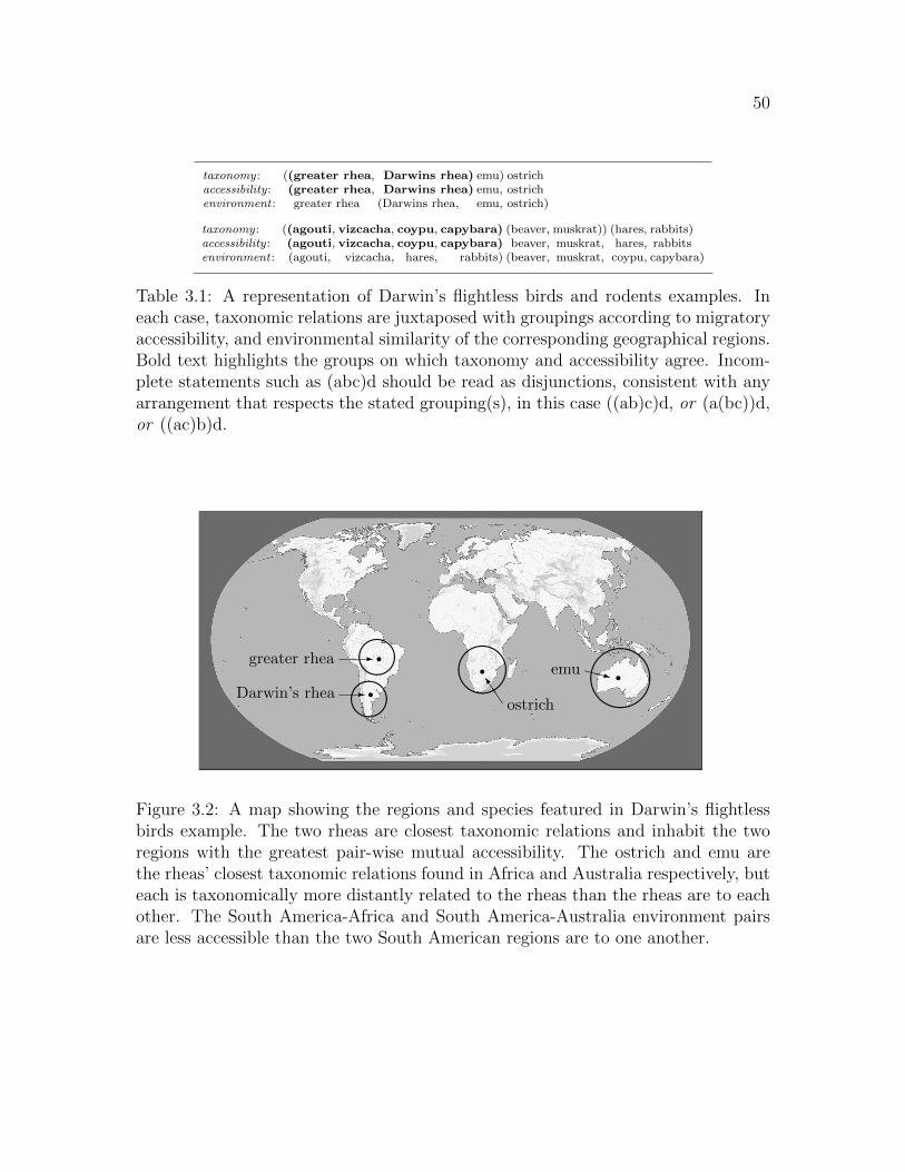
50

taxonomy: ((greater rhea, Darwins rhea) emu) ostrichaccessibility: (greater rhea, Darwins rhea) emu, ostrichenvironment : greater rhea (Darwins rhea, emu, ostrich)

taxonomy: ((agouti, vizcacha, coypu, capybara) (beaver, muskrat)) (hares, rabbits)accessibility: (agouti, vizcacha, coypu, capybara) beaver, muskrat, hares, rabbitsenvironment : (agouti, vizcacha, hares, rabbits) (beaver, muskrat, coypu, capybara)

Table 3.1: A representation of Darwin’s flightless birds and rodents examples. Ineach case, taxonomic relations are juxtaposed with groupings according to migratoryaccessibility, and environmental similarity of the corresponding geographical regions.Bold text highlights the groups on which taxonomy and accessibility agree. Incom-plete statements such as (abc)d should be read as disjunctions, consistent with anyarrangement that respects the stated grouping(s), in this case ((ab)c)d, or (a(bc))d,or ((ac)b)d.

����

Darwin’s rhea r����

greater rhea r����

ostrich

r&%'$

emu r-

-

JJ]

XXz

Figure 3.2: A map showing the regions and species featured in Darwin’s flightlessbirds example. The two rheas are closest taxonomic relations and inhabit the tworegions with the greatest pair-wise mutual accessibility. The ostrich and emu arethe rheas’ closest taxonomic relations found in Africa and Australia respectively, buteach is taxonomically more distantly related to the rheas than the rheas are to eachother. The South America-Africa and South America-Australia environment pairsare less accessible than the two South American regions are to one another.

51

the same order of Rodents,7 but they plainly display an American type

of structure. We ascend the lofty peaks of the Cordillera and we find an

alpine species of bizcacha; we look to the waters, and we do not find the

beaver or muskrat, but the coypu and capybara, rodents of the American

type. (349)

The phrase ‘American type’ refers to the morphological similarities that mark the

South American rodents as closest taxonomic relations. Regarding environmen-

tal similarity, the agouti and vizcacha have the same general external appearance

(‘habit’) as the hares and rabbits of Eurasia and North America, making them fit for

the same environments (Darwin appears to reason), while the semi-aquatic coypu and

capybara occupy roughly the same environmental niche as the beaver and muskrat

in North America. Thus accessibility relations again mirror the taxonomic relations,

while grouping by similarity of environment conflicts with taxonomy (see the bottom

half of Table 3.1).

I can summarize my reading of the ‘great facts’ by starting from the ground floor

observations and working up to the ‘high-level’ ones. (For brevity, I do this only for

the second and third facts.) The simplest observations each report the geographi-

cal range of a single species (or somewhat larger taxon). Darwin’s flightless birds

illustration, for example, includes four such observations, reporting the geographical

ranges of Darwin’s rhea, the greater rhea, the ostrich, and the emu.

7Rabbits and hares were moved out of Rodentia and into the sister order Lagomorpha in theearly 20th century. This development doesnt undermine Darwins argument. (There are closertaxonomic relations in Europe and America, but these are still taxonomically more distant thanthe South American rodents are to each other.)

52

Combined with some knowledge of the organisms’ migratory capabilities, the

simple location observations determine which species are, from their present locales,

more accessible to which other species. In the case of the flightless birds, the two

rheas (inhabiting neighboring regions of South America) make the most accessible

pair, while all other pairings (greater rhea with ostrich, ostrich with emu, etc.) are

considerably less accessible as the paired species inhabit different continents. These

accessibility relations can be summarized as per the ‘accessibility’ row of Table 3.1,

where placement inside parentheses indicates greater migratory accessibly with any-

thing else inside the parentheses than with anything outside. Notice that this sum-

mary statement says nothing about where any of the species are found. The summary

statement leaves behind information that was present in the simple observations, and

expresses an abstract feature of the whole set of simple observations.

Next, the abstract summary of accessibility relations is compared with preex-

isting, off-the-shelf taxonomic classifications for the same taxa. (Far from raw,

naive observations, these taxonomic classifications are themselves the products of the

theory and practice of biological taxonomy applied to observations of comparative

morphology—but I bracket discussion of how taxonomists produced these classifi-

cations, since here Darwin simply takes these products for granted.) Continuing

with the flightless birds example, the abstract summary of accessibility relations is

seen to be congruent with the taxonomic relations (i.e., the accessibility and taxo-

nomic arrangements contain some of the same groupings, and do not cross-cut one

another) as displayed in Table 3.1. The statement of congruence between taxonomic

and accessibility groupings now expresses a very abstract feature of an even larger

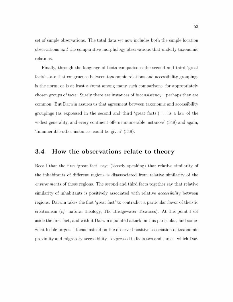
53

set of simple observations. The total data set now includes both the simple location

observations and the comparative morphology observations that underly taxonomic

relations.

Finally, through the language of biota comparisons the second and third ‘great

facts’ state that congruence between taxonomic relations and accessibility groupings

is the norm, or is at least a trend among many such comparisons, for appropriately

chosen groups of taxa. Surely there are instances of inconsistency—perhaps they are

common. But Darwin assures us that agreement between taxonomic and accessibility

groupings (as expressed in the second and third ‘great facts’) ‘. . . is a law of the

widest generality, and every continent offers innumerable instances’ (349) and again,

‘Innumerable other instances could be given’ (349).

3.4 How the observations relate to theory

Recall that the first ‘great fact’ says (loosely speaking) that relative similarity of

the inhabitants of different regions is disassociated from relative similarity of the

environments of those regions. The second and third facts together say that relative

similarity of inhabitants is positively associated with relative accessibility between

regions. Darwin takes the first ‘great fact’ to contradict a particular flavor of theistic

creationism (cf. natural theology, The Bridgewater Treatises). At this point I set

aside the first fact, and with it Darwin’s pointed attack on this particular, and some-

what feeble target. I focus instead on the observed positive association of taxonomic

proximity and migratory accessibility—expressed in facts two and three—which Dar-

54

win takes to support his own hypothesis. In the previous section I described those

observations rigorously; now I discuss their relation to Darwin’s hypothesis of com-

mon ancestry, and to some alternative hypotheses.

3.4.1 Darwin’s hypothesis

What is Darwin’s common ancestry hypothesis? It says that all species, extant and

extinct, trace back to one or a few common ancestor species. But it says more than

this. I think Darwin’s common ancestry hypothesis is best understood as an inter-

pretation of the taxonomic arrangements produced by the biological classification of

his time. Groups-within-groups taxonomic arrangements express relative taxonomic

‘relatedness’. But what did ‘relatedness’ mean? What is classification really about?

Minimally, a given classification was both a summary of observed morphological sim-

ilarities, and a predictive hypothesis regarding similarities in traits not yet observed,

or not taken into account in making the classification. Beyond this superficial agree-

ment, different naturalists had different ideas about the true nature of taxonomic

relations. A taxonomic classification might represent a blueprint in the mind of the

creator, or a map of the physiologically possible adult forms, or it might indicate the

constraints inherent in the embryological development of living organisms (Winsor

2009). Or—at least for varieties within a species, and perhaps even species within

a genus—taxonomic relations might express genealogical relations among the taxa.

As (Winsor 2009, 44) explains:

To us it may seem paradoxical that naturalists should use the word ‘re-

lated’ without agreeing on its meaning, but actually this tolerance en-

55

abled them to make progress as a scientific community.

The situation of naturalists in this period can be compared to that of contemporary

philosophers vis-a-vis ethics. Two philosophers can agree that ‘murder is wrong’,

even while entertaining different theories about what it means for an act to be wrong.

They agree on an ethical claim while disagreeing about meta-ethics. Naturalists be-

fore Darwin could and often did agree on classification claims even as they disagreed

about (so to speak) meta-classification.

Every groups-within-groups classification can also be represented as a branching

tree structure (see Figure 3.3). Many naturalists already believed that subgroups

within the same species, or even the same genus, were related genealogically. View-

ing classifications as trees, some of the twigs at the very tips of the tree were already

taken to indicate genealogical relations. Darwin pushed this interpretation to the

extreme, claiming that classifications were genealogical all the way down. All (or al-

most all) living things are related by genealogy, he said, and the closer the taxonomic

relation, the more recent the shared ancestor. In summary, Darwin’s common ances-

try hypothesis says: that all living things trace back to one or a few common ancestor

species, that the ancestry of life has the form of a branching tree, and that the shape

of this tree is revealed (at least approximately) in the taxonomic classifications of

Darwin’s time.

3.4.2 Were Darwin’s hypothesis correct

Now supposing this hypothesis were true, why should we expect to see the association

of taxonomic relatedness and migratory accessibility expressed in facts two and three?

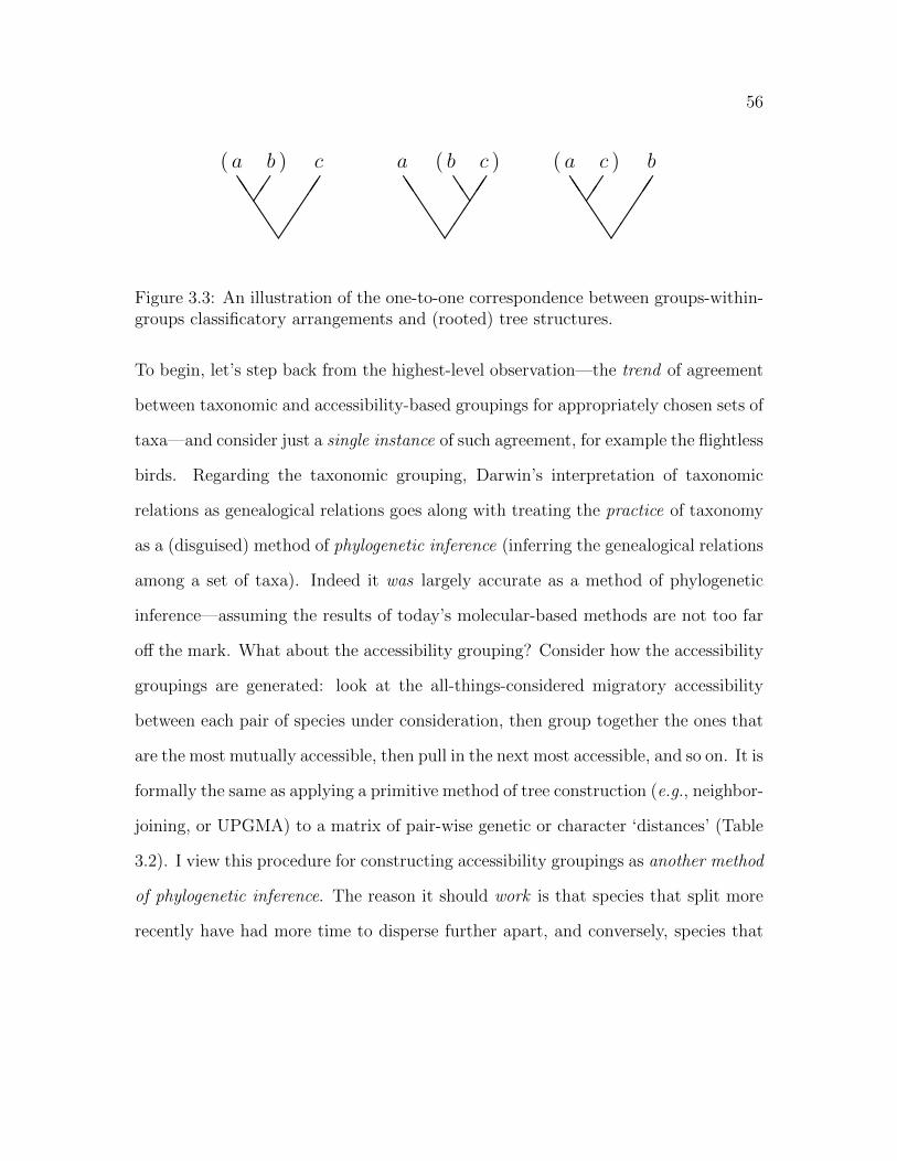
56

( a b ) c

JJJJJ

a ( b c )

JJJJJ J

J

( a c ) b

JJJJJ

Figure 3.3: An illustration of the one-to-one correspondence between groups-within-groups classificatory arrangements and (rooted) tree structures.

To begin, let’s step back from the highest-level observation—the trend of agreement

between taxonomic and accessibility-based groupings for appropriately chosen sets of

taxa—and consider just a single instance of such agreement, for example the flightless

birds. Regarding the taxonomic grouping, Darwin’s interpretation of taxonomic

relations as genealogical relations goes along with treating the practice of taxonomy

as a (disguised) method of phylogenetic inference (inferring the genealogical relations

among a set of taxa). Indeed it was largely accurate as a method of phylogenetic

inference—assuming the results of today’s molecular-based methods are not too far

off the mark. What about the accessibility grouping? Consider how the accessibility

groupings are generated: look at the all-things-considered migratory accessibility

between each pair of species under consideration, then group together the ones that

are the most mutually accessible, then pull in the next most accessible, and so on. It is

formally the same as applying a primitive method of tree construction (e.g., neighbor-

joining, or UPGMA) to a matrix of pair-wise genetic or character ‘distances’ (Table

3.2). I view this procedure for constructing accessibility groupings as another method

of phylogenetic inference. The reason it should work is that species that split more

recently have had more time to disperse further apart, and conversely, species that

57

split more recently can’t have gotten too far apart since their speciation.8 So long

as grouping taxa on the basis of pair-wise migratory accessibility has some value

as a method of phylogenetic inference, then its results should tend to agree with

taxonomic relations simply because they are two ways of inferring the same thing.

emu

ostrich

g.rhea

D.rhea

Darwin’s rhea 2 2 1 ·greater rhea 2 2 ·

ostrich 2 ·emu ·

Table 3.2: Pairwise migratory accessibility (using cartoon numbers) arranged todisplay the formal identity with a matrix of pair-wise character ‘distances’ as usedby some methods of tree construction. The two rheas are the most accessible, whileall other pairs are about equally (and much less) accessible. (For simplicity, I assumethat migratory accessibility is symmetric.)

This discussion connects directly back to the coin-tossing example. In that ex-

ample the simple, lowest-level observations were the individual coin toss outcomes

(heads, heads, tails, etc.). And there were two sets of these simple observations: A

and B. In Darwin’s biogeography observations, the two data set are (1) the set of

simple geographical location observations that underly the accessibility groupings,

and (2) the set of morphological observations that underly taxonomic classifications.

In the coin-tossing example, my hypothesis was that both data sets were generated

by tossing the same coin (with unknown bias). Just as that hypothesis is silent about

whether heads or tails is more probable on any individual coin toss, Darwin’s com-

mon ancestry hypothesis has nothing to say about where any particular organism

8For a more formal argument, see Sober’s probabilistic reconstruction of Darwin’s ‘space-timeprinciple’ (Sober 2008, 326)

58

should be found on the globe, or what morphological characteristics an organism

should display.

Now let’s step up one level of abstraction. Just as the frequency of heads in

one data set is a summary of the data that abstracts away from the individual coin

toss outcomes, an accessibility grouping such as ((D.rhea, g.rhea) ostrich, emu) is a

summary of, and a function of, a set of simple location observations. My ‘single-coin’

hypothesis in the coin-tossing example is silent about what frequency of heads should

be observed in either data set, when one or the other data set is viewed in isolation.

In the same way, when geographical distribution is viewed in isolation, Darwin’s

common ancestry hypothesis has no commitment to taxa being distributed in a way

that corresponds to any particular grouping. Likewise, if morphology is looked at in

isolation, the common ancestry hypothesis is (before the results of taxonomists are

known) equally compatible with any taxonomic arrangement.

When it comes to the difference between the frequency of heads in A and B,

my ‘single-coin’ hypothesis does make a commitment, it predicts that this value

should be near zero. The frequency of heads in A is not just any abstract feature of

data set A, it is the best (maximum likelihood) estimate of the coin’s probability of

landing heads on any given toss. Similarly, the frequency of heads in B is the best

estimate of the probability of landing heads for the coin that generated data set B.

My ‘single-coin’ hypothesis says that these two numbers are estimates of the same

quantity, so the difference between them should be small (see Note 2 for mathematical

details). In the same way, Darwin’s common ancestry hypothesis says that the

taxonomic classification and the accessibility grouping for the four flightless birds

59

are two estimates for which tree is the true genealogical tree that underlies both the

simple morphological observations and the simple geographical location observations.

Thus the two groupings should be the same, or at least similar. Congruence between

the taxonomic classification and the partial grouping based on accessibility is the

analogue of a small value for the difference-between-frequencies statistic in the coin-

tossing example.9

Finally, we have the highest-level observation: the trend of agreement between

taxonomic and accessibility groupings, as expressed in facts two and three through

the language of biota comparisons. Darwin doesn’t say exactly how often consistency

is observed as opposed to inconsistency—the rodents and birds are two examples of

consistency, and ‘Innumerable other instances could be given’, but there are surely

also many examples of inconsistency. I will characterize this highest-level observa-

tion conservatively, as agreement between taxonomic and accessibility groupings, for

appropriately chosen taxa, at a frequency greater than chance (where we can under-

stand ‘chance’ as the frequency that would result from drawing a grouping uniformly

at random from all possible groupings, and having that agree with the taxonomic

classification).10 To summarize very broadly, my claim is that this highest-level ob-

9A tighter analogy can be established by introducing a quantitative measure of the degree ofsimilarity between two trees. See, e.g., Robinson and Foulds (1981); Penny et al. (1982); Pennyand Hendy (1985) for such measures.

10More precisely, treat the accessibility grouping as drawn uniformly at random from among allpossible groupings that are comparably complete. For example, Darwin’s flightless birds illustrationfeatures 4 taxa and a single 2-member accessibility grouping. The number of distinct 2-membersubsets is

(42

)= 4!

2!(2!) = 6, but only one is consistent with the taxonomic classification. Such

agreement should occur ‘by chance’ only 1 in 6 times. The rodents illustration features 8 taxa anda single 4-member accessibility grouping. The number of distinct 4-member subsets is

(84

)= 8!

4!(4!) =

70. Such agreement should occur ‘by chance’ only 1 in 70 times. (Adding a fifth South Americanrodent—an alpine species of viscacha appearing in Darwin’s example but left out of the main text

60

servation should be observed, were Darwin’s common ancestry hypothesis correct.

Were congruence observed at or below chance, this would be surprising, and difficult

to reconcile with Darwin’s hypothesis. For those who use ‘predicts’ in the formal

sense that does not imply anything about the sequence of events in time, Darwin’s

common ancestry hypothesis predicts this observation.

3.4.3 Objections

Before moving on to consider some competing hypotheses and how those relate to

the same geographical distribution observations, I should address two objections to

the preceding analysis.

First objection: I have glossed both the taxonomic and the accessibility groupings

for a set of taxa (e.g., the flightless birds) as phylogenetic trees, each inferred from

a different data set. This gloss is an essential part of my argument that agreement

between the groupings is to be expected were Darwin’s common ancestry hypothesis

correct. But this talk of phylogenetic tress takes a very theory-laden perspective

on the observations. Have I not begged the question against hypotheses that deny

evolution and common ancestry by describing the observations themselves in terms

that only an advocate of common ancestry could accept?

Response: Notice that the same objection could be raised in the coin-tossing

example. An intuitive way of understanding why the difference-between-frequencies

statistic should be near zero, were my ‘single-coin’ hypothesis correct, is to note that

in this case the two frequencies would be two estimates of the single coin’s bias, so

for simplicity—brings the ‘chance’ frequency to 1 in 126.)

61

they should be roughly the same. This perspective on the observation is theory-laden,

and would be unacceptable to anyone who rejects my hypothesis. But this doesn’t

change the fact that the difference-between-frequencies statistic itself is a perfectly

objective function of the data. The statistic itself is the observation; the added

gloss about agreement between two estimates of the same quantity is a theory-laden

explanation of what that statistic means and why certain values should be observed.

Similarly, an observation of agreement between taxonomic and accessibility groupings

is a function of morphology, geographical location, and migratory capacity. Darwin

and his opponents can agree about all of these things, and so they can agree about

the observations. My talk of two methods of phylogenetic inference is an added,

theory-laden explanation of what those groupings mean and why agreement is to

be expected (at least with frequency greater than chance) were Darwin’s common

ancestry hypothesis correct.

Second objection: My argument depends on the idea that a very crude method

of grouping taxa by migratory accessibility can function as a workable method of

phylogenetic inference. But in fact accessibility is typically a dreadful proxy for

genealogical relatedness. For example, North American bison are much, much more

closely related to the water buffalo of Asia than to the prairie dogs underfoot, not to

mention the prairie grass, the ants, the microbes in the soil. For almost any choice of

taxa, judging genealogical relatedness based on relative migratory accessibility would

do no better than putting all possible trees into a hat and reaching in blindfolded.

Response: Geographic distribution contains some information about genealogical

relations, but the world is small and migration is fast. The noise of dispersal quickly

62

obscures the signal of genealogy.11 Grouping by accessibility is indeed a very limited

method of phylogenetic inference. There is, however, a set of circumstances under

which it will perform best: pair-wise migratory accessibility will carry the most infor-

mation about genealogy where (1) at least some speciations within the tree are recent

(so that dispersal has not erased all trace of genealogy), and (2) observed differences

in migratory accessibility between species pairs is large (and thus less plausibly at-

tributed to accidents of dispersal). The observations that I have described above

include only sets of taxa that satisfy these circumstances. On my reading of Dar-

win’s biota comparisons, representative taxa should be among each other’s closest

taxonomic relations that are found in each locale—this arranges for (1). And Dar-

win’s emphasis on contrasting within-continent biota pairs versus between-continent

biota pairs (see fact three) accords with (2). Thus the way in which the regions

are chosen, and then the way in which taxa are chosen from those regions, works to

limit the sets of taxa that enter into the observations to those for which geographical

distribution is informative about genealogical relations.

3.4.4 Alternative hypotheses

I’ve argued above that the trend in agreement between taxonomic and accessibility

groupings, expressed jointly by Darwin’s ‘great facts’ two and three, is to be expected

were his theory of common ancestry correct. Can the same be said of the alternatives

to Darwin’s hypothesis?

11Somewhat more formally: supposing that daughter species disperse via probabilistically inde-pendent random walks, the likelihood function over all possible trees flattens out very quickly, sothat relative accessibility data no longer contains any information about phylogeny.

63

In connection with the first great fact, Darwin discusses an alternative theory of

geographical distribution, according to which each species came into existence as-is,

and in just the right environment for that species to thrive. Supposing this hypothesis

were true, would it follow that taxonomic and accessibility groupings should be sys-

tematically congruent? It would, if some additional assumptions were true: (1) that

species more closely related taxonomically were fit for more similar environments,

and (2) accessibility between regions were correlated with similarity of environment.

But neither (1) nor (2) is true. Given that accessibility between regions is (at least

at a large geographical scale) uncorrelated with similarity between the environments

of regions, this hypothesis arguably predicts that taxonomy-accessibility congruence

should occur at chance frequency, which fits very poorly the observations.

A more relaxed variant of the preceding biogeographical theory is implicit in

Darwin’s discussion of single versus multiple creation cites for a single species (what

I’ve called, in my overview of chapters eleven and twelve, Darwin’s “replies to ob-

jections”). This theory allows for different locations of origin for each species, and

even for different populations within a species, but it does not put any constraints

on where those locations should be. This theory is perfectly consistent with the ob-

served trend of accessibility-taxonomy congruence, but it would be equally consistent

with any possible geographical distribution observations.

A third alternative can do better, but is also more similar to Darwin’s own theory.

In Darwin’s time, some amount of evolution and common ancestry was generally

accepted. Few doubted, for example, that subspecies within a species, or varieties

within a species could trace back to a common ancestor population in the past.

64

Some went so far as to allow that species within a genus all evolved from a common

ancestor. Such limited common ancestry theories will generate the same expectations

about geographical distribution as Darwin’s theory, so long as the species included

within a single congruence observation all fall within the same subspecies, species,

or genus, according to how much evolution and common ancestry the particular

alternative theory allows.

In Darwin’s description of the rodent example (p. 51 above) he notes that the

lowest taxonomic rank that includes all of the taxa taking part in the congruence is

the order. This is two full Linnaean ranks above genus. So the trend of congruence

between taxonomic and geographical groupings does hold for at least some groups of

taxa broad enough to discriminate between Darwin’s very general common ancestry

hypothesis and the more limited ones accepted by many of his contemporaries. But

for all that the geographical distribution observations have to say, it would remain

open for an opponent of Darwin’s general common ancestry theory to accept only

as much common ancestry and evolution as is indicated by the smallest inclusive

taxonomic rank of the taxa that participate in the trend. Ultimately, the limit of

the ability of the biogeographical evidence to distinguish between Darwin’s general

common ancestry hypothesis and more conservative variants of it is determined by

the limit of the method of inferring a genealogical tree from pairwise migratory acces-

sibility observations, as discussed above in the second objection of § 3.4.3. (Darwin

does not discuss this limit, nor these limited common ancestry hypotheses.)

65

3.5 Phylogenetic congruence

Before concluding, I wish to briefly point out how my analysis of Darwin’s geo-

graphical distribution observations places the form of those observations into the

context of modern evolutionary biology. The agreement between genealogical trees

inferred for the same taxa from different data sets, as described above, will be rec-

ognized by contemporary evolutionary biologists as a form of (what is now called)

‘phylogenetic congruence’. Phylogenetic congruence simply means the congruence

of two genealogical trees, each inferred from a different data set. The innumerable

instances of observed taxonomy-geography congruence summarized by Darwin’s sec-

ond and third great facts is each a qualitative and perhaps somewhat crude analogue

of the measures of tree similarity (Robinson and Foulds 1981) used in tests of phy-

logenetic congruence in contemporary phylogenetic systematics (Huelsenbeck et al.

1996), historical biogeography (Wiley 1988), symbiotic evolution (Funk et al. 2000),

and several other subfields of evolutionary biology. Darwin’s congruences are dif-

ferent, however, in that each of these modern types of congruence (including those

of modern biogeography) uses morphological or genetic data for both trees, while

Darwin’s congruences use morphological data for one tree and geographical data for

the other.

3.6 Conclusion

I have offered a new analysis of Darwin’s geographical distribution observations, and

of how those observations relate to Darwin’s theory of common ancestry. I take

66

these observations to support Darwin’s theory of shared ancestry over the alterna-

tives discussed above in virtue of Darwin’s theory predicting those observations (no

implication regarding the sequence of events in time intended) while the alternatives

either predict much less taxonomy-geography congruence or make no predictions and

are equally compatible with any amount of congruence. My analysis stands in con-

trast to those cited in § 3.1, according to which Darwin’s theory does not tell us

what we should expect to observe in nature were the theory correct. The novelty of

my analysis has two main sources. First, I’ve taken to heart the lesson illustrated by

the coin-tossing example from section 3.1, namely that a hypothesis can sometimes

stick its neck out regarding certain abstract, or ‘high-level’ features of a set of obser-

vations even while generating no expectations about any individual datum within

the set. And second, I have characterized the major trends from Darwin’s survey of

geographical distribution in a novel way that identifies just such a ‘high-level’ obser-

vations (or ‘patterns’), namely the congruences of accessibility-based groupings with

taxonomic relations for appropriately chosen groups of taxa.

67

Part II

Diversity

68

Chapter 4

The Confirmational Significance of

Agreeing Measurements

4.1 Introduction

The agreement of independent measurements occurs when a theoretically posited

quantity is measured via multiple, and (in some sense) ‘independent’ methods, and

those measurements agree (cf. Forster 1988). The phenomenon is also called ‘the

method of overdetermination of constants’ (Norton 2000), and ‘the consilience of

inductions’ (Whewell 1858/1989a). Judging by the scientific episodes most studied

and celebrated by philosophers, the phenomenon is of central importance to confir-

mation in science. The agreement of independent measurements played a key role in

confirming, e.g., Newton’s theory of gravity (Forster 1988; Harper 2007), the wave

theory of light (Whewell 1858/1989a), Darwin’s theory of common ancestry (Chap-

69

ter 3 of this dissertation), the atomic theory of matter (Salmon 1984; Norton 2000),

the charged particle (electron) theory of cathode rays (Norton 2000), and the theory

of plate tectonics (Koolage 2008). In the present essay I propose a new, formal ac-

count of the phenomenon’s epistemic significance, and contrast my proposal with a

more established approach to the same problem.

The agreement of independent measurements is often treated under the ‘diversity

of evidence’ heading (where the ‘independence’ of individual measurements is taken

to enhance the ‘diversity’ of a total set of observations that includes those measure-

ments). But that approach (in its current form) does not adequately acknowledge

the hierarchical structure that is characteristic of hypothesis spaces in science. Spe-

cific scientific hypotheses are nested within more general hypotheses, and those are

nested within hypotheses more general still. Within such a structured hypothe-

sis space, the diversity of evidence approach locates the evidential significance of

agreeing measurements at the nitty-gritty level of parameter estimates—agreement

warrants extra confidence that the measured value is accurate. While not incor-

rect, this result is incomplete, and does little to explain the perceived significance of

agreeing measurements in the history of science. My proposal complements existing

accounts by identifying, in addition, warrant for the ‘higher level’ theory that posits

the measured quantity. It is the confirmation of this higher level hypothesis—more

so than the very specific hypothesis that a parameter takes a certain value—that

explains the historical significance of the real scientific examples.

Regarding formal methodology, I will judge the evidential import of an observa-

tion via the Law of Likelihood (Hacking 1965; Edwards 1984; Royall 1997). That is, I

70

treat an observation as supporting one hypothesis over another if that observation is

more probable supposing the one hypothesis were correct, compared with supposing

the other hypothesis were correct. More formally, observation o favors hypothesis h1

over hypothesis h2 if: p(o|h1) > p(o|h2). Likelihoodists and Bayesians of all stripes

can agree that such comparisons are the basis of confirmation. I wish to bracket the

finer, quantitative issues about how strongly a hypothesis is favored or confirmed by

an observation (Fitelson 2011). My proposal concerns the more basic issue of exactly

which hypotheses and observations to label o, h1, and h2, such that the import of

agreeing measurements can be better appreciated within the framework of Bayesian

epistemology broadly understood.

4.2 Examples of the Phenomenon to be Analyzed

A couple of examples will indicate the flavor of the phenomenon to be analyzed. The

following quotations from (Whewell 1858/1989a), and (Norton 2000), frame scientific

work by Thomas Young and Jean Baptiste Perrin respectively:

And what was no less striking a confirmation of the truth of the [wave]

theory [of light], Measures of the same element deduced from various

classes of facts were found to coincide. Thus the Length of a luminiferous

undulation, calculated by Young from the measurement of Fringes of

shadows, was found to agree very nearly with the previous calculation

from the colours of Thin plates. (Whewell 1858/1989a, 154)

. . . Perrin was able to report roughly a dozen different methods for es-

71

timating N [Avogadro’s number] and they all gave values of N in close

agreement. In the conclusion to Les Atoms, Perrin tabulated the result-

ing estimates of N from methods based on: viscosity of gases (kinetic

theory), vertical distribution in dilute emulsions, vertical distribution in

concentrated emulsions, Brownian movement . . . , density fluctuations in

concentrated emulsions, critical opalescence, blueness of the sky, diffusion

of light in argon, black body spectrum, charge of microscopic particles,

radioactivity . . . (Norton 2000, 73)

As Norton paraphrases Perrin’s argument, ‘The case for the reality of atoms and

molecules lay in this agreement . . . ’ (Norton 2000, 73). Although each individual

measurement of N concerns the size of the atom, the agreement of these measure-

ments is said to confirm the general theory that matter consists of atoms (also see

Salmon 1984). Similarly, in the first quotation above, Whewell says that agreement

between two measurements of the wavelength of light confirms the theory that light

is made of waves (not the more specific hypothesis that lightwaves have such and

such length).

It is this type of inference—confirmation for the higher level theory, based on

agreeing measurements of a quantity posited within the theory—that I will recon-

struct formally in what follows. Again, this is not to deny that such agreement can

also confirm the measured value for the quantity posited within the theory, if that

theory is already taken to be true. But Perrin’s main conclusion was that matter

is made of atoms. Young’s main conclusion was that light is a wave. (Analogous

statements hold for the other examples from §1.)

72

4.3 Measurement Formally Characterized

To begin my analysis of the agreement of measurements, I first abstractly characterize

the phenomenon itself. I formally characterize measurement as the statistical proce-

dure of parameter estimation. Parameter estimation requires a statistical model—a

family of probability distributions, each associated with a particular value for the

model’s adjustable parameter (or with a vector of values, if the model has multiple

parameters). Given a set of data, the highest likelihood distribution (or distribu-

tions) within the family can be identified, and the associated parameter value (or

interval) is the parameter estimate. On this characterization of measurement, the

statistical model’s adjustable parameter is the quantity to be measured, and estima-

tion of that parameter’s value, as just described, is a measurement. For example,

suppose we want to measure the mass of an object using a spring scale. Like any

measuring device, our scale is imperfect. Suppose that its readings are normally dis-

tributed around the true mass of the object that is hung from it. This supposition is

the statistical model. We produce a set of data by hanging the object, observing the

reading, removing the object, then repeating the procedure a number of times. These

data are then used to estimate the mean of the normal distribution from which the

individual readings were treated as random draws. This estimate is a measurement

of the object’s mass.

What then, is the agreement of measurements? Suppose we have two disjoint

datasets, and a statistical model for each. The two models needn’t be the same,

and each may include adjustable parameters that the other does not, but they must

both contain an adjustable parameter representing the quantity to be measured.

73

Each model is fitted to its respective data set, generating two vectors of parameter

estimates, and two estimates of the shared parameter, i.e., two measurements of the

quantity to be measured. (I understand ‘agreement’ between measurements as a

matter of degree, and I will quantify this precisely in the worked example below.)

Continuing with the spring scale example, suppose we measure the mass of the

same object again, this time (as astronauts are ‘weighed’ in space) by applying a

known force to the object, observing its resulting motion, calculating acceleration,

and finally working back to the object’s mass by applying f = m × a. In this

case the data are a set of (position, time) points, and the statistical model is a

Newtonian equation of motion with a stochastic element representing observation

error. The object’s acceleration is estimated from these data via the model, and mass

is calculated from acceleration and force. This estimate is a second measurement of

the object’s mass. (While the two example measurements just described—the spring

scale and the applied force—are intuitively ‘different’, or ‘independent’ methods, note

that I have not yet characterized the ‘independence’ of measurements. I address this

in what follows.)

4.4 Agreement as Observation

With the phenomenon formally characterized, I turn to its epistemic significance.

I first illustrate my approach using the simplest possible case of the agreement of

measurements. Say we will make two measurements of the mass of an object, us-

ing two separate spring scales. Let there be two data sets with 20 points each

74

xa = {x1, x2, . . . , x20} and xb = {x21, x22, . . . , x40}, corresponding to forty scale read-

ings, twenty from each scale, all using the same object. For each data set employ

the location-normal model with known variance σ2 = 1, and unknown mean µ. I.e.,

model a says that the twenty points xa are drawn from twenty independent and

identically distributed random variables {X1, X2, . . . , X20}, each normal with vari-

ance σ2 = 1, and mean µa. Model b says the same about points x21 − x40, with

mean µb. Under the location-normal model, the maximum-likelihood estimator for

the value of µ is the mean of the data set. So the two maximum-likelihood estimates

for the true values of µb and µb are xa and xb respectively.

Now I introduce a super-model that expresses the assumption, required for the

agreement of measurements, that xa and xb are two estimates (measurements) of the

same quantity. This super-model is the location-normal model treating all forty ran-

dom variables {X1, X2, . . . , X40} as independent, with identical normal distributions,

with variance σ2 = 1 and mean µ (µ = µa = µb). And to quantify the degree of

agreement between the two measurements of the parameter µ, I define the following

statistic of the total data set {x1, x2, . . . , x40}: xa − xb. The closer this statistic is

to zero, the greater the agreement between measurements. Call this the agreement

statistic.1 What does the super-model predict about the value of the agreement

statistic? With respect to the super-model, this particular statistic is what is called

ancillary, meaning that the probability assigned to observed values of the statis-

tic does not depend on the value of the adjustable parameter. By definition, such

1I don’t mean to privilege the formula xa − xb over other ways of quantifyingagreement, e.g., |xa−xb|, or (xa − xb)2. Either of these alternatives can be substitutedfor the simple difference statistic used in the text without affecting my conclusions.

75

statistics contain no information about the parameter value, and are thus completely

useless for parameter estimation. The model itself assigns probabilities to observed

values of an ancillary statistic, regardless of the value of the model’s adjustable pa-

rameter. In the case of the statistic xa−xb and the super-model introduced above, it

is easy to understand why the super-model alone generates these probabilities. If all

40 random variables {X1, X2, . . . , X40} have the same distribution, then regardless of

what µ is, we should expect {x1, x2, . . . , x20} and {x21, x22, . . . , x40} to be clustered

around roughly the same value. Qualitatively, the super-model should assign higher

probability to values of the agreement statistic near zero, and assign lower probabil-

ity to large positive or negative values. The actual distribution is shown as the solid

line in figure 4.1.

-2 -1 0 1 2

0.0

0.5

1.0

1.5

xa − xb

Density

Figure 4.1: Probability density distributions assigned to the agreement statistic bythe one-parameter (solid line) and two-parameter (dashed line) super-models. (Dis-tributions approximated via simulation.)

76

To summarize what I’ve done so far, I first treat measurement as parameter es-

timation, and the agreement of measurements as agreement between two estimates,

based on disjoint data sets, of a single parameter shared by two statistical models.

To formally encode the idea that the parameter appearing in both statistical models

is the same quantity, I introduce a super-model that comprises the two models plus

the assumption that µa = µb. Then I characterize the agreement of measurements

as a statistic of the total data (in this case xa − xb), and I treat the degree of agree-

ment itself as an observation. I must emphasize this last part because it is the key

to my approach. It may initially seem unintuitive (or worse) to treat the degree of

agreement between two estimates of a posited quantity as an observation. Admit-

tedly, it is a very abstract, ‘high-level’ observation. Yet the agreement statistic is a

straight-forward function of the total data set, and is thus entirely determined by

the data.2 And so long as we can calculate a probability function for the statistic,

nothing prevents us from treating it as an observation within our statistical frame-

work. For my simplest-case example, I have displayed the probability distribution

assigned to the agreement statistic by the super-model. My next step is to introduce

a competing super-model, and calculate the distribution that it assigns to the same

agreement statistic. I will then locate the epistemic significance of the agreement

of independent measurements in the likelihood favoring of the one super-model over

the other, given observed values of the agreement statistic near zero.

2Compare the ‘higher-level regularities in the data’ in Forster’s (1988) discussion ofWhewellian methodology, Sober’s (1999) observation of ‘matching’ character statesbetween two species, and the treatment of differences between AIC scores in Forsterand Sober (2011).

77

4.5 A Competing Super-model

Let’s temporarily set aside the super-model discussed above, and go back to the two

data sets xa = {x1, x2, . . . , x20} and xb = {x21, x22, . . . , x40}, and the two separate

location-normal statistical models with known variance σ2 = 1, and unknown means

µa and µb respectively. (Recall the example of a single object weighed twenty times

on each of two spring scales.) Now I introduce an alternative super-model. I want

this alternative to lack the commitment to a common mechanism underlying the

two data sets, so where previously I assumed that µa = µb, now I remove that

constraint. This alternative super-model is simply a composite of the two separate

location-normal models, which retains both adjustable parameters µa and µb. Call

the original super-model the one-parameter super-model, and call this alternative

the two-parameter super model.

What does the two-parameter super-model say about the agreement statistic

xa − xb? The agreement statistic is not ancillary for the two-parameter model,

meaning that the distribution assigned to that statistic depends on the values of

the adjustable parameters µa and µb. All on its own, the two-parameter super-model

doesn’t say enough—it is too logically weak—to predict anything about that statistic.

We can, however, use a standard Bayesian technique to generate a distribution over

the agreement statistic by logically strengthening the two-parameter super-model hy-

pothesis. We can assume prior probability distributions for the parameters µa and µb,

and then ‘integrate out’ those priors. Think of this logically strengthened hypothesis

as describing two layers of stochastic processes. The data {x1, x2, . . . , x40} are gen-

erated by first drawing values for µa and µb from their respective prior distributions,

78

and then drawing data points {x1, x2, . . . , x20} and {x21, x22, . . . , x40} from normal

distributions with means µa and µb respectively. The first level of stochastic processes

is intended to represent uncertainty about the true values of the parameters, and the

two-level process incorporates that uncertainty into the super-model’s predictions

about the data. Adding priors in this way logically strengthens the two-parameter

super-model enough to generate predictions about the agreement statistic, and I

employ this procedure in order to contrast the two super-models vis-a-vis observed

values for the agreement statistic.

Exactly what the augmented two-parameter super-model predicts about the agree-

ment statistic of course depends on what priors are built into that hypothesis. But

qualitatively, the likelihood comparison between the two super-models is not very

sensitive to the choice of priors. Here is one example calculation. For convenience,

I start by assuming that the priors for µa and µb are normal, and independent. Let

the variance of each distribution be σ2 = 25 to represent a moderate degree of un-

certainty about those parameter values. The resulting distribution assigned to the

agreement statistic further depends only on the difference between the means of the

two prior distributions, not on their individual values. The smaller the difference

between the two means, the more the two-parameter super-model predicts agree-

ment between measurements, so it is most charitable to make the difference zero.

Intuitively, the resulting distribution over the agreement statistic should be fairly

flat, since the high variance in the first level of the stochastic process means there

is a large range of reasonably probable divergences between µa and µb, and so the

probability mass is spread more widely over possible values for xa − xb. The actual

79

distribution is shown as the dashed line in figure 4.1. (The distribution is centered

on zero only because I have made the means of the two priors equal.)

Comparing the two distributions pictured in figure 4.1, the one-parameter super-

model has much higher likelihood for observed values of the agreement statistic

near zero. It is this likelihood comparison between the two super-models which, on

my account, expresses the epistemic significance of the agreement of independent

measurements.3

4.6 Application

So far I have provided a concrete illustration, framed in abstract mathematical terms.

It remains to be explained how the competing hypotheses that are salient within the

real scientific episodes characterized as ‘the agreement of independent measurements’

are relevantly similar to the two super-models from my illustration.

The real world analogues of the one-parameter super-model are hypotheses that

posit a quantity that is not (colloquially speaking) directly observable, but can (ac-

3Regarding sensitivity to the choice of priors, any difference between the meansof the two priors will shift the mean of the resulting distribution for the agreementstatistic away from zero, making the likelihood comparison with the single-parametersuper-model even more dramatic. The effect of increasing or decreasing the varianceof the priors depends on how close the two means are, but the likelihood of the two-parameter super-model, given an observed value of the agreement statistic near zero,can approach that of the one-parameter super-model only if the variance of the priorsis very low, and their means are very close to one another. In subjective terms thismeans that the agent is very confident that µa = µb in which case the two-parametersuper-model collapses to the one-parameter super-model; in this case it is no concernthat comparing likelihoods no longer distinguishes the two hypotheses.

80

cording to its hypothesized nature) be measured in multiple ways. For example, in

Newton’s physics the mass of an object can be measured by observing how much the

object stretches a spring, or by observing how much it accelerates when a force is

applied (§3). Likewise, the wave theory of light posits a wavelength, and the atomic

theory of matter posits a number of particles in a standard unit of a substance.

Each posited quantity was (eventually) measurable in a variety of ways. These are

the one-parameter hypotheses.

The real-world analogues of the two-parameter super-model are harder to charac-

terize as a group since these hypotheses vary a great deal in how fully and explicitly

they are articulated. They lie on a scale from full-fledged alternative scientific theory

to vague skeptical worry. Despite the variation exhibited in that dimension, I will

endeavor to explain how they all share the relevant similarity to the two-parameter

super-model from my illustration. To do this, I must go back and discuss an aspect

of my formal illustration that I glossed over in the first pass.

Returning to the formal illustration, consider the dual nature of the quantity xa,

the mean value of the data set xa = {x1, x2, . . . , x20}. On the one hand, xa is the

maximum-likelihood estimate of the value of the parameter µa. Call this the theoreti-

cal perspective on xa. But at the same time, xa is merely the result of a mathematical

operation applied mechanically to the data set xa. Call this the observational per-

spective on xa. Notice that while the two super-models share the same observational

perspective on xa, they take contradictory theoretical perspectives on xa. We might

say that they offer different interpretations of xa. The one-parameter super-model

interprets xa as the best estimate of the single parameter µ which also underlies data

81

set xb = {x21, x22, . . . , x40}. The two-parameter super-model interprets xa as the

best estimate of the parameter µa (which parameter exerts no influence on data set

xb—the stochastic process underlying data set xb being governed by a separate pa-

rameter µb). The common thread among real world analogues of my two-parameter

super-model is that they offer a more limited, local interpretation of a single mea-

surement.

On the full-fledged scientific theory end of the spectrum, take for example the

Ptolemaic theory of the solar system as an alternative to the Copernican theory.

Ptolemy put the Earth at the center of the solar system, and decomposed the ap-

parent motion of each planet (as viewed from Earth) into an orbit around Earth

(the deferent), plus a second, smaller orbit (the epicycle) that circles a point moving

along the deferent. It turns out that the Ptolemaic epicycle captures the component

of apparent planetary motion that is in fact contributed by the motion of the Earth

around the Sun. In effect, Ptolemy (unknowingly) took the motion of the Earth

around the Sun and displaced it to another location within his picture of the solar

system—but another location from which it could make the same contribution to the

overall motion of a planet relative to the Earth. Thus the relative motion of the Sun

and Earth is replicated within the Ptolemaic model for each planet. A Ptolemaic

‘super-model’ addressing two planets plus the Earth will then include one parameter

for the period of the first planet’s epicycle, and another parameter for the period of

the second planet’s epicycle. The corresponding Copernican super-model, however,

will treat the estimates of those two parameter values as two estimates of the same

quantity, viz., the period of the Earth’s orbit around the Sun.

82

At the other end of the spectrum we have less fully articulated ideas about a mea-

surement being an ‘artifact’ of the measuring procedure, or the measuring device,

or of the particular experimental setup generating the data (cf. Hacking 1985). The

single-parameter hypothesis interprets the measurement as an estimate of a property

of the entity under study, which property will naturally be constant across repeated

measurements or measurements using different techniques. The alternative ‘hypoth-

esis’ interprets the measurement as a property of the dust on the microscope lens,

or of a glitch in the computer software, or of a one-off spike in emissions from the

factory down the road, i.e., as an estimate of some quantity that is of less general

significance and that would not be expected to influence attempted measurements

of the target property on other occasions or through other media. Fully articulating

such alternative hypotheses would involve positing separate parameters underlying

the results of separate measurement attempts on other occasions or through other

media, as per the two-parameter super-model in my illustration.

4.7 Evidential Diversity?

Now that my proposal is on the table, I contrast it with an alternative approach to

the same problem, and say where I think that approach falls short. For purposes of

formal analysis, the agreement of independent measurements is usually lumped under

the rubric of ‘evidential diversity’. The literature on evidential diversity is a response

to the widely experienced intuition that collections of confirming observations that

are more ‘diverse’, ‘varied’, or ‘heterogeneous’ (or, equivalently, the parts of which

83

are ‘independent’ or ‘of different kinds’) confirm a hypothesis more strongly than

otherwise comparable collections that are ‘narrow’, ‘homogeneous’, or ‘of the same

kind’. Hempel’s discussion of the ‘criteria of confirmation and acceptability’ provides

a standard expression of the idea. Hempel first discusses how, as the number of

supporting observations already cited grows larger, the confirmation effected by a

new supporting observation grows smaller. He then adds the following caveat:

This remark must be qualified, however. If the earlier cases have all been

obtained by tests of the same kind, but the new finding is the result

of a different kind of test, the confirmation of the hypothesis may be

significantly enhanced. For the confirmation of a hypothesis depends

not only on the quantity of the favorable evidence available, but also on

its variety: the greater the variety, the stronger the resulting support.

(Hempel 1966, 33–34)

Notice how Hempel sets up the problem. He addresses a set of observations each

of which individually confirms the hypothesis in question, and then gestures at a

notion of ‘variety’ within such sets, and a relationship between this ‘variety’ and the

sum total of confirmation provided by the set. The challenge is then to rigorously

define the ‘variety’ (or related property) of a collection of individually confirming ob-

servations in such a way that one’s normative epistemic theory (typically Bayesian

epistemology) pronounces a hypothesis better confirmed when the supporting ob-

servations have more of that property (e.g., Sober 1989; Earman 1992; Howson and

Urbach 1993; Wayne 1995; Fitelson 2001; Bovens and Hartmann 2003).

84

The observations and hypotheses in my illustration above do not satisfy (or at

least need not satisfy) this setup. Recall that the competing hypotheses in my

example were the one- and two-parameter super-models for the total data set x =

{x1, x2, . . . , x40}. What the diversity of evidence approach calls the observations

would be those associated with the two ‘independent’ measurements, viz., xa and xb

(or xa and xb, the difference will not matter). The problem is that neither of these

observations individually confirms the one-parameter super-model. If you look at

only one half of the total data set, e.g., xa = {x1, x2, . . . , x20}, the two super-models

say exactly the same thing about those data (and about any statistic of those data).

Both supermodels say that xa = {x1, x2, . . . , x20} came from 20 independent and

identically distributed random variables, each normal with known variance σ2 = 1,

and unknown mean. The only difference between the two super-models is whether

that mean is given by the parameter µa or the parameter µ, but this difference

is immaterial if we restrict our attention to xa. (The same can be said, mutatis

mutandis, of xb.)

In terms of the spring scale example from §3, the one-parameter hypothesis says

that two different scales measure the same property, and the two-parameter hypoth-

esis says that the two scales measure different properties, or at least may measure

different properties. Naturally, weighing an object on only the first scale does not

discriminate between the two hypotheses. (And neither does weighing an object on

only the second scale.) More formally, neither super-model (all on its own) assigns

any probability to xa. A likelihood comparison vis-a-vis xa can be made by adding

prior distributions over both µa and µ and calculating likelihoods as per the proce-

85

dure described in §5. But if those two priors are the same, as would seem to facilitate

a fair comparison, then the two super-models will assign exactly the same probabil-

ity to xa (and to any other statistic of xa). Thus, neither measurement favors one

super-model over the other. The way that I have identified the relevant observations

and hypotheses puts the inference problem that I am addressing outside of the set

up to which the diversity of evidence literature is addressed.

The diversity of evidence approach may address some of the same scientific sce-

narios, but focusses on a different aspect of the problem by directing attention to

different hypotheses and observations. In contrast to my treatment of the agreement

between measurements as an observation (in the form of the agreement statistic),

the diversity of evidence approach treats each individual measurement as an obser-

vation. The question is then: What do xa and xb each individually confirm? If

we set aside the two-parameter super-model, and assume that the one-parameter

super-model is correct, then similar observed values for xa and xb each confirm a

similar range of values for the parameter µ (recall that x is the maximum-likelihood

estimate of µ for the normal model). It is at this point that the issues raised in

the quotation from Hempel become relevant. How ‘diverse’ is the observation set

{xa, xb}, (or, equivalently, how ‘independent’ are xa and xb)? And how ought this

degree of diversity impact our beliefs about the true value of the parameter µ? The

key point here is that treating the two measurements as each confirming the same

value (or range of values) for the parameter µ presupposes the one-parameter hy-

pothesis, whereas what I have tried to show is how the agreement of measurements

confirms the one-parameter hypothesis.

86

Mapping this distinction back onto the motivating scientific examples, the diver-

sity of evidence approach presupposes the wave theory of light, and then addresses

how ‘diversity’ among measurements helps confirm a value for the wavelength. The

diversity of evidence approach presupposes the atomic theory of matter, and ad-

dresses confirmation for hypotheses about the size of the atom. The diversity of evi-

dence approach presupposes the Copernican model of the solar system, and addresses

confirmation for hypotheses about the period of the Earth’s orbit. In contrast, I have

tried to show how agreement between measurements of the wavelength of light can

confirm the wave theory of light, how agreement between measurements of the size

of the atom can confirm the atomic theory of matter, and how agreement between

measurements of the period of the Earth’s orbit can confirm the Copernican model

of the solar system.

4.8 Conclusion

Seeing that multiple, ‘independent’ measurements of a quantity agree, one intuitive

conclusion is that the value about which the measurements agree is correct (and

moreover, the greater the ‘independence’, the more confidence is warranted). But

there is another, more basic (yet less obvious) conclusion, which is equally intuitive

once made explicit: that the several procedures used for measurement in fact measure

the same property. The first conclusion, which is the subject of the diversity of

evidence literature, presupposes the second. I have pointed to historically detailed

philosophical work suggesting that the second conclusion is at least as important

87

as the first within the scientific episodes that are described as the agreement of

independent measurements and which partially motivate the diversity of evidence

literature. I have provided a template for formal reconstruction and rationalization

of this second and more basic element within the motivating scientific episodes. The

key innovation is to treat the degree of agreement between measurements as a single

observation (a statistic of a total data set). Hypotheses that posit a single property

underlying multiple measurement attempts will tend to assign a higher probability

to close agreement between measurements, as compared to hypotheses that posit

different parameters underlying different measurement attempts.

88

Chapter 5

Evidential Diversity in

Hierarchically Structured

Hypothesis Spaces

5.1 Introduction

In the previous chapter, I introduced an approach to modeling the epistemology

of agreeing measurements, and very briefly contrasted this approach with existing

philosophical work on the related topic of evidential diversity. In the present chapter

I generalize this approach to agreeing measurements to directly address the epis-

temic intuition motivating the diversity of evidence literature, namely that a set of

supporting observations that is diverse in character provides better evidence than

an otherwise comparable set of supporting observations that lacks diversity or is “all

89

the same kind”. This will involve defining “diversity” and explaining in what sense

diverse evidence is “better” evidence. Existing formal work on the value of diverse

evidence uses the Bayesian framework predominantly, and I will adopt that frame-

work here, and discuss in detail how the account that I present compares to existing

Bayesian work on the diversity of evidence.

The real scientific examples that I take to motivate interest in the epistemological

problem that I am addressing include some of those mentioned in the introduction to

Chapter 4. But they also include countless more mundane examples from both sci-

ence and everyday reasoning. These are the kind of examples that I discussed at the

end of § 4.6, in which the alternative hypotheses are usually expressed informally as

worries about the reliability of a method of measurement, rather than as alternative

scientific theories. As an example of such a more mundane instance, consider the

famous episode of Florin Perier’s measurement of the height of a column of mercury

in an early barometer, at the top of the Puy de dome.

The Puy de dome is a high lava dome in south-central France, and Perier was

the brother-in-law of Blaise Pascal. Pascal wanted to know how mercury-column

readings at high altitude compared to those made near sea level, and Perier lived

near the Puy de dome, so Pascal asked Perier to make the trek, and the reading, for

him. Perier and an entourage scaled the dome and made the measurement. But not

just one measurement:

To make sure they took measurements in five places at the top, on one

side and the other of the mountain top, inside a shelter and outside, but

the column heights were all the same. (Boring 1954)

90

The result of the measurement (i.e., the height of mercury observed) was very signifi-

cant to Pascal’s broader theorizing about hydrostatics, but setting aside this broader

scientific importance of the result, notice that to get that result, Perier et al. made a

number of separate measurements under diverse conditions at the top of the dome.

5.2 Formal Example

5.2.1 Setup

I will continue to use parameter estimation as a general model of measurement.

Because it is intuitive and accessible, I begin with an example using coin tossing (i.e.,

the geometric statistical model). Consider some observations of coin toss outcomes

{t, h, h, . . .}. Suppose we have four methods of collecting such data, methods A, B,

C, and D. And suppose that 20 outcomes are collected by each method. (Ultimately,

I will call the four data sets different “kinds” of observation, and say that the total

data set is “diverse” in virtue of including these several kinds.) Now consider four

hypotheses about the process(es) that generated these data, hypotheses 1–4. All

four hypotheses agree that the data represent the outcomes of coin tosses. But they

disagree in what are called their homogeneity assumptions.

Two data sets are homogeneous with respect to a given statistical property if

that property is constant across those data sets. For example, (labeling the data set

gathered by collection method A as a, that gathered by collection method B as b,

and so on) the frequency of heads might be the same in data sets a and b, in which

case those data sets are homogeneous with respect to that statistical property. We

91

must, however, distinguish between the sample frequency and the coin’s probability of

landing heads. The former is the observed frequency of heads in the actual data; the

latter is the corresponding property of the process that generated the data. (In the

long run, the two have the same value, but in small data sets they may diverge due to

sampling error.) Homogeneity typically refers to processes rather than outcomes, in

which case data sets a and b may be homogeneous despite small differences in their

sample frequencies—in other words, it is the probability of heads that is constant

across the two data sets.

Continuing to spell out the hypotheses, about data collected by any single col-

lection method all four hypotheses say the same thing: that each coin toss is an

independent draw from the distribution p(heads) = θ, p(tails) = θ − 1, where θ is

unknown but constant. The four hypotheses disagree about whether θ is constant

across data collection methods. Using θi to indicate p(heads) for data collected by

method i, hypothesis 1 says that θa = θb = θc = θd. The other hypotheses make

different homogeneity assumptions, as depicted in Table 5.1; each partitions the

total data into at least two parts, and allows for different values for p(heads) within

different parts of the total data. To complete the probabilistic description of the four

hypotheses, let each say that the θi are drawn from a uniform probability density

distribution over the interval [0,1]. Where θi and θj are not constrained to be equal,

they are treated as independent draws from the uniform distribution.

92

A B C Dhypothesis 1 θa = θb = θc = θdhypothesis 2 θa = θb = θc θdhypothesis 3 θa = θb θc θdhypothesis 4 θa θb θc θd

Table 5.1: Hypotheses 1–4 make different homogeneity assumptions. Hypothesis1 says that p(heads) is constant across all four data collection methods, whereashypothesis 4 says that p(heads) may be (and probably is) different for each method.Hypotheses 2 and 3 are intermediate in how much they partition the total data intoparts inhomogeneous with respect to p(heads).

5.2.2 Analysis

Now I wish to show, given the above setup, how a kind of evidential diversity can be

important to the relative confirmation of hypotheses 1–4. Recall that 20 coin toss

outcomes are collected by each of four data collection methods. Suppose that the

observed frequencies of heads in those four data sets are: a = 0.4, b = 0.5, c = 0.35,

and d = 0.4. The observations that I will consider are comparisons between these

four observed frequencies. Representing heads by 1 and tails by 0, the frequency

of heads in data set x is the average of the values in the set, written as x. The

observations I will consider are the observed values of the following statistics of the

total data: |a− b|, |a− c|, and |a− d|. Given the frequencies supposed above, those

values are: 0.1, 0.05, and 0, respectively. (What is important for my purposes in

these numbers is only that the four frequencies fall within a small range, so that the

difference statistics are nearish to zero.)

I’ll begin with a simple, qualitative analysis of what these observations say about

hypotheses 1–4, and then move on to a rigorous Bayesian treatment. Consider the

93

observation that |a− b| = 0.1. Roughly, such a small difference in frequency between

data sets a and b is what we should expect to see supposing any of the hypotheses

that constrain θa and θb to be equal. Hypotheses 1–3 all include that constraint.

Hypothesis 4, on the other hand, says that θa and θb are independent draws from the

uniform distribution over [0,1], on which supposition such a small difference between

a and b is at least somewhat less probable. So the first observation reflects equally

well on hypotheses 1–3, and somewhat less well on hypothesis 4. In the same way,

the observed small value for |a − c| is just what we should expect supposing any

hypothesis that constrains θa and θc to be equal (those being hypotheses 1 and 2),

but a bit of a coincidence on hypotheses that treat θa and θc as independent draws

from the uniform distribution (hypotheses 3 and 4). Finally, the difference between

a and d is also small, and this observation is more favorable to hypothesis 1 than

to any of the other hypotheses since only by hypothesis 1 requires θa and θd to be

equal.

The formal Bayesian analysis of the example follows the outlines of the informal

one just given. Figure 5.1 displays the probability distributions that sinlge-theta and

independent-theta hypotheses assign to all possible values of the statistics |a − b|.

By “single-theta” I mean hypotheses 1–3, all of which assume that data collected by

methods A and B are homogeneous with respect to p(heads). For the statistic |a−b|,

hypothesis 4 is the only “independent-thetas” hypothesis, meaning that hypothesis

4 treats data collected by methods A and B as generated by two values of p(heads),

drawn independently from the uniform distribution over [1,0]. The corresponding

probability distributions for statistics |a− c| and |a− d| are exactly the same; what

94

changes, in proceeding from one statistic to the next, is only which of hypotheses A,

B, C, and D count as single-theta and which count as independent-theta hypotheses.

Drawing all likelihoods from Figure 5.1, and assuming a uniform prior over the four

hypotheses to begin with, Figure 5.2 displays the posterior probabilities for those

hypotheses after sequential conditionalization on the observations that |a− b| = 0.1,

|a− c| = 0.05, and |a− d| = 0.

To compare this example to that from the previous chapter, the important con-

ceptual difference so far is that in last chapter’s example, there were two hypotheses

with different homogeneity assumptions (though I didn’t use that term there), as

opposed to the four hypotheses in the current example. The “one-parameter super-

model” treated the whole data set as homogeneous with respect to the parameter µ,

while the “two-parameter super-model” partitioned the total data in two. The latter

hypothesis treated each half of the data as internally homogeneous with respect to

µ, while treating the whole data set as (potentially) inhomogeneous. In the current

example each of four hypotheses posits different homogeneity assumptions. Now I

introduce a second important difference.

The mathematical example in the previous chapter concerned the contrast be-

tween how two hypotheses (the one- and two- parameter super-models) related to

a single data set. The difference in how those two hypotheses related to the total

data set could be described as a difference in how much each hypothesis unified those

data. And more generally, this is the kind of contrast that is relevant to characteriz-

ing unification, namely two hypotheses compared via their relations to the same data

set. Implicit in Figure 4.1 (page 75) is a second kind of contrast, a contrast between

95

0.0 0.2 0.4 0.6 0.8 1.0

0.0

0.1

0.2

0.3

0.4

Two probability distributions over |a − d|

difference in frequency

probability

equal thetasindependent thetas

Figure 5.1: Two probability functions over possible values for the statistic |a−b|. Thepicture is exactly the same for the statistics |a− c|, and |a− d|. What changes fromobservation to observation is how many of the four hypotheses are “equal thetas”versus “independent thetas” for the relevant data collection methods. Likelihoodsfor each step of Bayesian conditionalization come from this plot (specifically, fromthe values at “difference in frequency” = 0.0, 0.05, and 0.1).

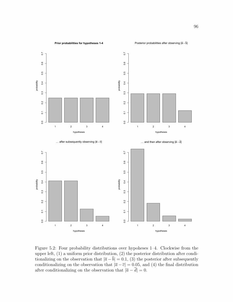
96

1 2 3 4

Prior probabilities for hypotheses 1-4

hypotheses

probability

0.0

0.1

0.2

0.3

0.4

0.5

0.6

0.7

1 2 3 4

Posterior probabilities after observing |a − b|

hypotheses

probability

0.0

0.1

0.2

0.3

0.4

0.5

0.6

0.7

1 2 3 4

… after subsequently observing |a − c|

hypotheses

probability

0.0

0.1

0.2

0.3

0.4

0.5

0.6

0.7

1 2 3 4

… and then after observing |a − d|

hypotheses

probability

0.0

0.1

0.2

0.3

0.4

0.5

0.6

0.7

Figure 5.2: Four probability distributions over hypoheses 1–4. Clockwise from theupper left, (1) a uniform prior distribution, (2) the posterior distribution after condi-tionalizing on the observation that |a− b| = 0.1, (3) the posterior after subsequentlyconditionalizing on the observation that |a− c| = 0.05, and (4) the final distributionafter conditionalizing on the observation that |a− d| = 0.

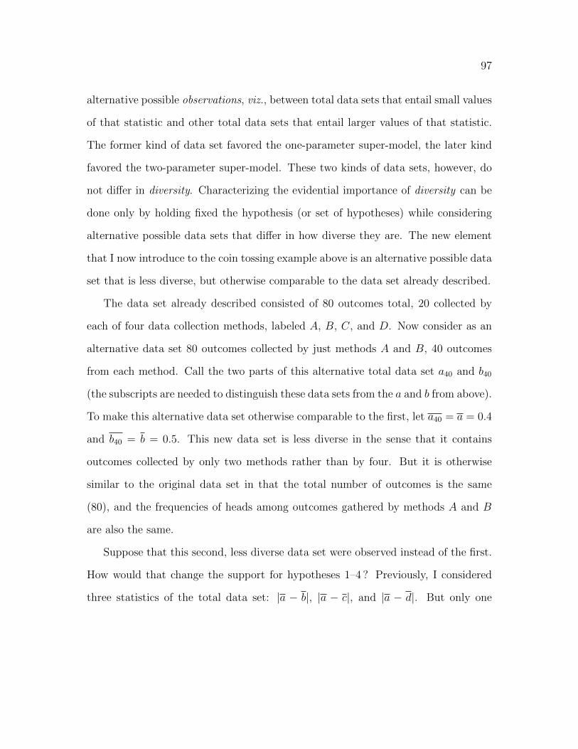
97

alternative possible observations, viz., between total data sets that entail small values

of that statistic and other total data sets that entail larger values of that statistic.

The former kind of data set favored the one-parameter super-model, the later kind

favored the two-parameter super-model. These two kinds of data sets, however, do

not differ in diversity. Characterizing the evidential importance of diversity can be

done only by holding fixed the hypothesis (or set of hypotheses) while considering

alternative possible data sets that differ in how diverse they are. The new element

that I now introduce to the coin tossing example above is an alternative possible data

set that is less diverse, but otherwise comparable to the data set already described.

The data set already described consisted of 80 outcomes total, 20 collected by

each of four data collection methods, labeled A, B, C, and D. Now consider as an

alternative data set 80 outcomes collected by just methods A and B, 40 outcomes

from each method. Call the two parts of this alternative total data set a40 and b40

(the subscripts are needed to distinguish these data sets from the a and b from above).

To make this alternative data set otherwise comparable to the first, let a40 = a = 0.4

and b40 = b = 0.5. This new data set is less diverse in the sense that it contains

outcomes collected by only two methods rather than by four. But it is otherwise

similar to the original data set in that the total number of outcomes is the same

(80), and the frequencies of heads among outcomes gathered by methods A and B

are also the same.

Suppose that this second, less diverse data set were observed instead of the first.

How would that change the support for hypotheses 1–4 ? Previously, I considered

three statistics of the total data set: |a − b|, |a − c|, and |a − d|. But only one

98

of those statistics can be formulated in this second scenario, namely |a − b|. By

stipulation, that statistic has the same value that it did in the original scenario. Just

as before, the small observed value for |a− b| is more probable on those hypotheses

that make θa = θb than on those that treat θa and θb as independent draws from

the uniform distribution [0,1]. The former include hypotheses 1–3, the latter only

hypothesis 4. So hypotheses 1–3 are favored over hypothesis 4. But the import of

the evidence ends there. Without outcomes gathered by methods C and D, there are

no observations that could possibly discriminate between hypotheses 1–3; all three

hypotheses say exactly the same thing about all possible data gathered by methods

A and B. So the evidential difference between the original and less diverse data

sets is seen in the range of alternative hypotheses over which the observations favor

hypothesis 1. The more diverse set of observations favors hypothesis 1 over each of

the other three, while the less diverse set favors hypothesis 1 over hypothesis 4, while

leaving hypotheses 2 and 3 on par with hypothesis 1.

More formally, starting again with a uniform prior over hypotheses 1–4, the pos-

terior distribution after conditionalization on the observation that |a40− b40| = 0.1 is

exactly the same as that after observing |a− b| from the original, more diverse data

set, i.e., the upper right plot of Figure 5.2.1

1The two posteriors are the same because, for all i, j, and x:

p(|a40 − b40| = x∣∣hypothesis i)

p(|a40 − b40| = x∣∣hypothesis j) =

p(|a− b| = x∣∣hypothesis i)

p(|a− b| = x∣∣hypothesis j)

despite that for all x and i:

p(|a40 − b40| = x∣∣hypothesis i) 6= p(|a− b| = x

∣∣hypothesis i)

99

5.3 “Diversity” and “Kinds”

On the approach to evidential diversity just illustrated, what counts as “diverse”?

What does it mean for observations to be “different kinds”? On this approach,

neither term applies to observations on their own. Rather, “diversity” and “kinds”

are defined only relative to the set of hypotheses under consideration. Two data

sets are different kinds of data if any of the hypotheses under consideration say that

they are by partitioning the total data set into parts and treating those parts as

inhomogeneous with respect to the measured quantity (or potentially so), where the

two data sets in question come from different parts of the partition. Roughly, an

observation set is more diverse the more such partitions of the total observation set

are stipulated by salient competing hypotheses.

5.4 Application

The formal example above can be mapped schematically onto the case of Perier’s

mercury tube measurements mentioned in § 5.1. Recall that Perier made a series of

measurements under varying circumstances at the top of the peak: in a sheltered area

and out in the open, and on different sides of the peak. These differing circumstances

of measurement correspond to the different data collection methods A, B, C, and D

in my formal example. From the perspective of hypothesis 1 in the formal example,

each observed frequency (a, b, c, and d) is a measurement of the single quantity θ.

Each of hypotheses 2–4, on the other hand, treats one or more of b, c, and d as

something other than an additional measurement of the quantity measured by a.

100

What about the hypotheses 1–4 ? The Perier analogue of hypothesis 1 is the

hypothesis that all of the measurements made at the top of the Puy de dome are

measurements of the same theoretically posited quantity: the air pressure at that

altitude. In other words, that hypothesis treats observations collected at the dif-

ferent locations as homogeneous with respect to the measured quantity. The other

hypotheses are ones that posit some heterogeneity within that total observation set.

For example, one possible alternative hypothesis says that mercury tube readings are

influenced significantly by whether they take place on the windward or the leeward

side of the peak. Another says that sunlight influences the readings. Every such

hypothesis partitions the total data set into parts that are generated by somewhat

different underlying processes, like hypotheses 2–4 in the formal example.

Perhaps a more accurate formalization of such alternative hypotheses as the one

that has sunlight influencing the mercury height would include a parameter for air

pressure that is constrained to be constant across measurement contexts, but where

each context introduces additional parameters that also influence the result of the

reading. I have avoided this in my formal example only for simplicity of presentation.

There are many ways to instantiate statistical heterogeneity. For present purposes,

in terms of the likelihoods displayed in Figure 5.1, the effect should not be very

different.

101

5.5 The Correlation Approach

In the rest of this chapter I give a brief overview of the main strand of existing

Bayesian literature on evidential diversity, and explain how what I’ve said so far fits

into that literature. This is the approach to modeling the epistemology of evidential

diversity that Wayne (1995), Steel (1996), and Bovens and Hartmann (2003) call the

“correlation approach”.

Speaking in terms of similarity between observations (where an observation set is

less diverse the more similar its constituent observations are to one another) Howson

and Urbach (1993) write:

This idea of similarity between items of evidence is expressed naturally in

probabilistic terms by saying that e1 and e2 are similar provided P (e2|e1)

is higher than P (e2); and one might add that the more the first probability

exceeds the second, the greater the similarity. This means that e2 would

provide less support if e1 had already been cited as evidence than if it

was cited by itself. (159–60)

Granted the stipulated relations between e1 and e2, their claim that e2 would provide

less support for h had e1 already been cited as evidence follows directly from the

Bayesian conditionalization rule, according to which the posterior probability of a

hypothesis h after making observation e2 is:

P (h|e2) = P (h)× P (e2|h)

P (e2)(5.1)

102

As P (e2) is the denominator of the factor P (e2|h)/P (e2) by which the prior prob-

ability of the hypothesis h is multiplied to arrive at the posterior probability of h,

increasing P (e2) decreases that posterior probability. In this way, h is better con-

firmed by observations e1 and e2 if those two observations are such that learning

e1 does not raise the probability of e2, as opposed to being such that learning e1

does raise the probability of e2. In short, the less similar e1 and e2, the more they

jointly confirm h. Earman (1992) points to the same mechanism for more “varied”

observation sets to confirm more strongly than less varied ones.

Wayne (1995) labeled the approach taken by Howson and Urbach (1993) and

Earman (1992) the “correlation approach”,2 and repackaged it by defining a measure

of similarity, S:

S(e1, e2) =p(e2|e1)p(e2)

=p(e1 & e2)

p(e1) p(e2), (5.2)

and more generally, for (e1, e2, e3, . . . en):

S(e1, e2, e3, . . . en) =p(e1 & e2 & . . . & en)

p(e1)p(e2) . . . p(en). (5.3)

Myrvold (1996) adopts S and further explores its role in Bayesian confirmation by

defining a “conditional form” of S:

S(e1, e2, . . . en|h) =p(e1 & e2 & . . . & en|h)

p(e1|h)p(e2|h) . . . p(en|h). (5.4)

2Strictly speaking, the term “correlation” is misused here. Correlation describes a relation-ship either between random variables, or between event types, while Wayne uses it to describe arelationship between individual events.

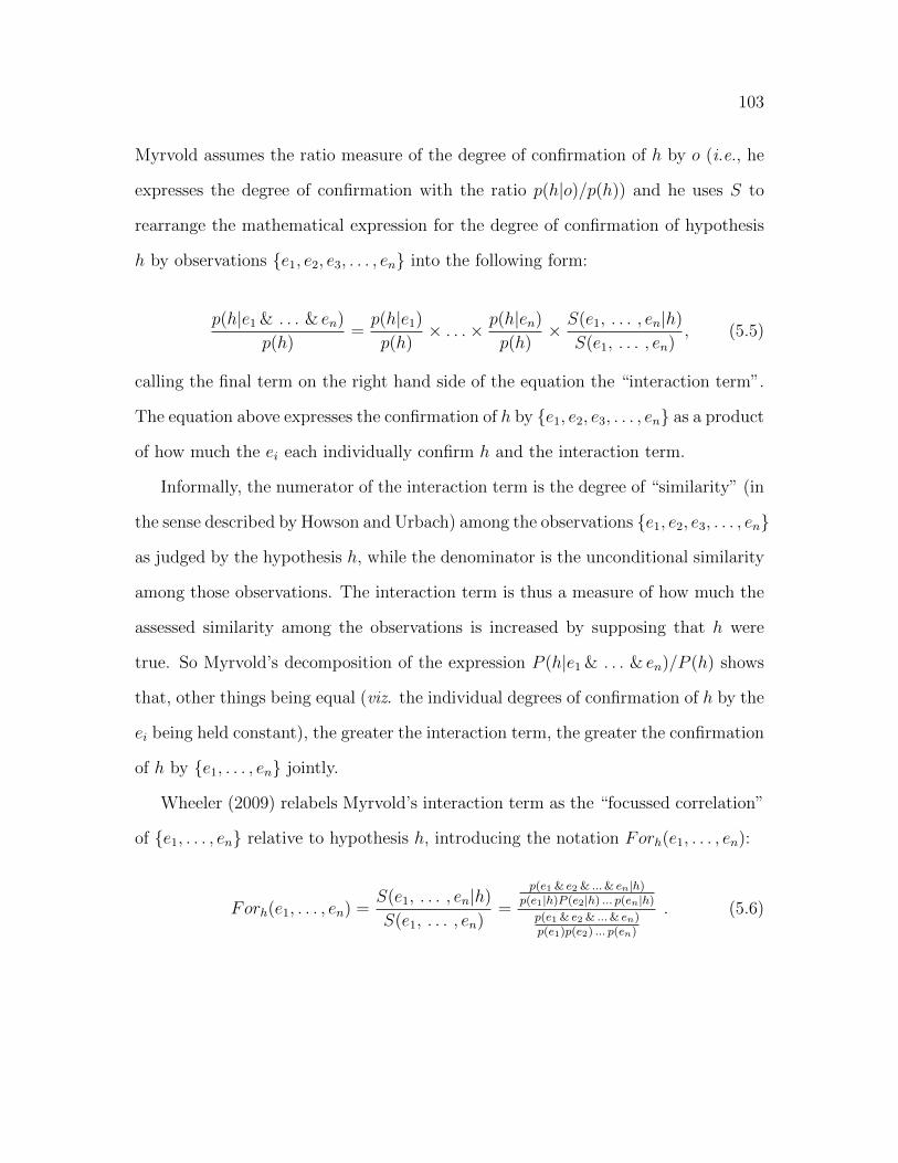
103

Myrvold assumes the ratio measure of the degree of confirmation of h by o (i.e., he

expresses the degree of confirmation with the ratio p(h|o)/p(h)) and he uses S to

rearrange the mathematical expression for the degree of confirmation of hypothesis

h by observations {e1, e2, e3, . . . , en} into the following form:

p(h|e1 & . . . & en)

p(h)=p(h|e1)p(h)

× . . .× p(h|en)

p(h)× S(e1, . . . , en|h)

S(e1, . . . , en), (5.5)

calling the final term on the right hand side of the equation the “interaction term”.

The equation above expresses the confirmation of h by {e1, e2, e3, . . . , en} as a product

of how much the ei each individually confirm h and the interaction term.

Informally, the numerator of the interaction term is the degree of “similarity” (in

the sense described by Howson and Urbach) among the observations {e1, e2, e3, . . . , en}

as judged by the hypothesis h, while the denominator is the unconditional similarity

among those observations. The interaction term is thus a measure of how much the

assessed similarity among the observations is increased by supposing that h were

true. So Myrvold’s decomposition of the expression P (h|e1 & . . . & en)/P (h) shows

that, other things being equal (viz. the individual degrees of confirmation of h by the

ei being held constant), the greater the interaction term, the greater the confirmation

of h by {e1, . . . , en} jointly.

Wheeler (2009) relabels Myrvold’s interaction term as the “focussed correlation”

of {e1, . . . , en} relative to hypothesis h, introducing the notation Forh(e1, . . . , en):

Forh(e1, . . . , en) =S(e1, . . . , en|h)

S(e1, . . . , en)=

p(e1 & e2 & ...& en|h)p(e1|h)P (e2|h) ... p(en|h)

p(e1 & e2 & ...& en)p(e1)p(e2) ... p(en)

. (5.6)

104

Wheeler (2009); Wheeler and Scheines (2011); Schlosshauer and Wheeler (2011)

investigate the relationship between focussed correlation and confirmation. Wheeler

and Scheines (2011) show that given assumptions (a) and (b) below, for hypothesis h

and evidence sets e = {e1, e2} and e∗ = {e1, e3}, if the focussed correlation of e by h

is greater than that of e∗ by h, then the confirmation of h by e is greater than that by

e∗, on any one of several of common measures of confirmation. The conditions are:

(a) that the ei each individually confirm h, and (b) that P (h|ei) = P (h|ej) for all

i& j. (On the ratio measure, this result follows trivially from Mryvold’s equation; the

result of Wheeler and Scheines (2011) is more general.) Schlosshauer and Wheeler

(2011) relax assumption (b), and demonstrate that if Forh(e1, e2) is greater than

Forh(e1, e3) but e3 individually confirms h a lot more than e2 individually confirms

h, the higher individual confirmation within e∗ can outweigh the higher focussed cor-

relation of e, and e∗ will confirm h more strongly than e does. They give inequalities

that have to hold for better focussed correlation to entail better confirmation, and

vice versa.

5.5.1 My proposal and the correlation approach

The way that I have spelled out diversity among observations, and the value of

that diversity for confirmation, can also be modeled within the so-called correlation

approach. I will demonstrate this by recasting my coin example in terms of (using

Wheeler’s terminology) focussed correlation. Then I will discuss how my original

presentation differs in emphasis from the focussed-correlation reformulation, and

what I take my approach to add to the existing work on the correlation approach.

105

Viewing my coin example from the focussed correlation perspective, the relevant

observations are not the frequency differences |a − b|, |a − c|, and |a − d| as in

my earlier presentation of the example, but rather the full data sets: a, b, c, and

d, or instead (the results will be the same) the frequencies a, b, c, and d. The

upper right plot of Figure 5.3 (light colored bars) displays the results of starting

with a uniform prior over hypotheses 1–4 and conditionalizing not on the frequency

differences as I did previously, but on the conjunction a& b& c& d. The lower right

plot shows the results of instead conditionalizing on the observation: a40 & b40 (again

the lighter colored bars). The dark colored bars in the upper and lower right plots

repeat results from the corresponding earlier calculations for comparison, displaying

the posterior probabilities after conditionalizing on {|a − b|, |a − c|, |a − d|}, and

{|a − b|, |a − c|} respectively. As the comparisons show, there is little difference

in the posteriors between conditionalizing on the frequency differences (dark bars),

and conditionalizing on the frequencies themselves (light bars). The difference that

diversity makes to the posterior distribution (four kinds of observation versus two

kinds) is apparent using either approach to describing the observations.

Moreover, the focussed correlation values of the two different observation sets,

relative to each of hypotheses 1–4, do manage to express the features of the exam-

ple that lead to the posterior probabilities displayed in Figure 5.3. Returning to

Myrvold’s (1996) decomposition of the expression p(h|o)/p(h) (motivated by the ra-

tio measure of confirmation), plugging in the observation set {a, b, c, d}, and using

Wheeler’s (2009) notation for focussed correlation yields the following expression for

the degree of confirmation of hi by a& b& c& d :

106

1 2 3 4

Priors

hypotheses

probability

0.0

0.1

0.2

0.3

0.4

0.5

0.6

0.7

1 2 3 4

frequency differencesfull frequencies

Posteriors (four "kinds")

hypotheses

probability

0.0

0.1

0.2

0.3

0.4

0.5

0.6

0.7

1 2 3 4

Priors

hypotheses

probability

0.0

0.1

0.2

0.3

0.4

0.5

0.6

0.7

1 2 3 4

frequency differencesfull frequencies

Posteriors (two "kinds")

hypotheses

probability

0.0

0.1

0.2

0.3

0.4

0.5

0.6

0.7

Figure 5.3: Probability distributions over hypotheses 1–4. The top row shows uni-form prior distributions (left) and posterior distributions after conditionalizing onfour kinds of data (right). The bottom row shows uniform prior distributions again(left) and posterior distributions after conditionalizing on two kinds of data (right).The frequency difference statistics are used as the observations for the darker bars,whereas the frequencies themselves are the observations for the lighter colored bars.

107

p(hi|a& b& c& d)

p(hi)=p(hi|a)

p(hi)× p(hi|b)

p(hi)× p(hi|c)

p(hi)× p(hi|d)

p(hi)× Forhi

(a, b, c, d) (5.7)

The right hand side of Equation 5.7 can, in this particular case, be simplified, since

for all i

p(hi|a)

p(hi)=p(hi|b)p(hi)

=p(hi|c)p(hi)

=p(hi|d)

p(hi)= 1 , (5.8)

so the first four terms of the right hand side of Equation 5.7 can be ignored, and the

ratio of posterior to prior probabilities for any hi is simply equal to the value of the

focussed correlation expression Forhi(a, b, c, d).

Using the alternative, less diverse observation set {a40, b40}, Myrvold’s decompo-

sition of p(h|o)/p(h) becomes:

p(hi|a40 & b40)

p(hi)=p(hi|a40)p(hi)

× p(hi|b40)p(hi)

× Forhi(a40, b40) . (5.9)

Again, no individual observation confirms any hi on its own, i.e., for all i:

p(hi|a40)p(hi)

=p(hi|b40)p(hi)

= 1 . (5.10)

So the ratio of posterior to prior probabilities for any hi is again equal to the value of

the focussed correlation expression, Forhi(a40, b40). Table 5.2 displays the focussed

correlation values for both the four-kinds and the two-kinds observation sets, relative

to each of hypotheses 1–4. If you refer back to Figure 5.3, you can confirm that the

108

“full frequencies” posterior probabilities are, for each hypothesis, equal to the prior

times the focussed correlation from Table 5.2.

a,& b& c& d a40 & b40h1 2.671 1.176

h2 0.823 1.176

h3 0.349 1.176

h4 0.157 0.473

Table 5.2: The table displays eight values for the expression that Wheeler (2009)calls the “focussed correlation” of the observations relative to a hypothesis: that ofobservation sets {a, b, c, d} and {a40, b40} relative to hypotheses 1–4.

In short, what the preceding formulas and figures show is that the notion of

focussed correlation, already widely discussed in the literature, appears to adequately

capture the epistemically relevant differences between the four-kinds and two-kinds

data sets—what I have called a difference in diversity. Nonetheless, my analysis of

the four-hypothesis coin example goes beyond the existing literature in several ways.

While focussed correlation is a very abstract mathematical feature of theory-

observation relations, I have constructed a concrete example that actually generates,

from the ground up, the probabilistic relations required for two data sets to differ in

focussed correlation relative to a set of hypotheses. My concrete example can also

be schematically mapped onto numerous scientific and everyday examples that share

the relevant features of the Perier episode discussed in Section 5.1. I have built a

bridge between formalism and case study.

Moreover, my example expands the scope of the diversity of evidence literature

by demonstrating the application and relevance of both the concept of diversity and

109

the mathematics of the so-called correlation approach within a type of scenario that

falls outside of the topic’s usual domain. The standard idea is that the evidential

importance of diversity among observations comes into play in scenarios in which

the individual observations each already support or confirm the hypothesis in ques-

tion. Indeed this is an explicit assumption of the formal results derived in Wheeler

and Scheines (2011) and Schlosshauer and Wheeler (2011). But this assumption

is violated in my example; there, none of the individual observations confirms any

hypothesis over any other.3 The diversity within a set of observations can be epis-

temically relevant even where no individual observation is.

Finally, I have applied the formalism of Bayesian epistemology in a non-standard

way by identifying the key statistics of the full data set (the difference-between-

frequencies statistics), and treating those as the observations—feeding them into the

Bayesian updating mechanics rather than a more complete description of the data.

One attractive feature of this way of doing things is that the statistic of the data that

the formalism treats as the observation actually corresponds to what is intuitively

meaningful in those observations. In the coin example, it really doesn’t matter what

the frequencies themselves are (a, b, and so on); the hypotheses only differ on what

they predict about the frequency differences. Neglecting the identification of the key

data statistics and treating the frequencies themselves as the observations is to throw

a lot of irrelevant (or nearly irrelevant) information into the formalism—this does

less to illuminate the epistemology of the inference problem, even if the posterior

3This follows directly from the fact that p(obs.|hi) = p(obs.|hj) for all obs. ∈ {a, b, c, d, a40, b40}and all i ∈ {1, 2, 3, 4}. In Bayesian updating, there can be no change in posterior probabilitieswithout likelihood differences between hypotheses.

110

distribution that comes out the back end of the Bayesian updating mechanics is

nearly the same.

An additional consequence of treating the key data statistics as the observations

rather than using a more complete description of the data is that this shift can

reduce the influence of prior probabilities on the likelihoods p(obs.|hi) that govern

updating. Recall that in the example above, each of hypotheses 1–4 included one

or more parameters θ, and that in addition, each hypothesis stipulated a uniform

distribution over [0, 1] as the source of each parameter θ. I built in those uniform

distributions for simplicity, but real scientific hypotheses typically do not come with

probability distributions from which their parameters are drawn. In the absence of

such a distribution as a proper part of the hypothesis, Bayesian epistemology has

the agent’s subjective prior distribution over the parameter space do the job. The

larger the role of such priors in the updating process, the less objective the inference.

In the example above, when the observation is a difference-between-frequencies

statistic (e.g., |a−b|) and the hypothesis is a single-theta hypothesis for that statistic

(e.g., h1), the probability p(obs.|h) is hardly affected by the prior over θ. That is

because h1 predicts a small value for |a − b| regardless of what value θ takes. But

where the observation includes the frequencies themselves (e.g., a& b) the probability

p(obs.|h) now depends very heavily on the prior distribution over θ because p(obs.|h)

takes very different values for different values of θ, and that prior distribution deter-

mines how those widely differing values are weighted to establish the average value

of p(obs.|h) that will appear in the Bayesian updating factor. (But I have not yet

systematically investigated the influence of different priors on confirmation in such

111

scenarios, and I must leave that for another occasion.)

112

Wrap Up

Most of the concluding has already been done in the closing discussions of the pre-

ceding chapters. So here I will give a brief big-picture synopsis, with some reminders

about how the various parts connect to one another.

I began by criticizing Sober’s account of Darwin’s argument for common ancestry.

I argued that Sober’s reconstruction of how anatomical similarities provide evidence

favoring Darwin’s common ancestry (CA) hypothesis over a separate ancestry (SA)

alternative does not effect the theory comparison that it was designed to make. In-

stead it compares two logically stronger hypotheses: a specific version of CA against

a specific version of SA, where the more specific CA hypothesis is a high-likelihood

variant (relative to the other variants of CA) and the more specific SA hypothesis is

a low-likelihood variant (relative to the other variants of SA). If this characterization

of Sober’s likelihood comparison is accurate, then that comparison is not a rational

way to assess the evidence for the more general hypotheses CA and SA.

Still in Chapter 2, I went on to also criticize Sober’s application of modus Darwin

to geographical distribution observations. There I argued that while geographical

modus Darwin does frame a theoretically possible way to use geographical distribu-

113

tion observations to distinguish between the general CA and SA hypotheses, that

argument form does not suffice to model and illuminate Darwin’s more complex

geographical distribution argument.

From there I proceeded to give my own account of how morphological and geo-

graphical distribution observations relate to, and support Darwin’s universal common

ancestry hypothesis over some alternatives that posit a lesser degree of common an-

cestry (Chapter 3). On my account, they do so not independently (as per Sober)

but jointly, through “high-level” statistics of mixed (morphological + geographical)

observation sets. The relevant “high-level” feature is whether taxonomic and acces-

sibility groupings (trees) for the same set of taxa are congruent.

The congruence between trees inferred separately from different data sets can

be viewed as a special case of agreement between estimates of a parameter within

a statistical model, where the estimates are based on disjoint data sets. In Chap-

ter 4, I proposed this second description as a formal characterization of the theory-

observation relation variously known as the agreement of independent measurements,

the overdetermination of constants, and the consilience of inductions. I located the

epistemic significance of such agreement in the difference in likelihood, given a small

observed value of an agreement statistic, between those hypotheses that posit a single

parameter involved in generating both data sets and those that posit separate param-

eters underlying the two data sets (i.e., between hypotheses like the one-parameter

super-model and the two-parameter super-model).

In Chapter 5, I introduced the idea of the homogeneity assumptions of a hypothe-

sis in order to describe the important difference between the one-, and two-parameter

114

supermodels from the previous chapter, and I generalized the importance of that idea

through the analysis of an example in which each of four competing hypotheses make

different homogeneity assumptions. The homogeneity assumptions of those hypothe-

ses determine what observations will count as “different kinds” of observations in that

context, and are also responsible for the greater amount of confirmation that accrues

to hypotheses that treat more observation kinds as homogeneous with respect to the

measured parameter (so long as the various estimates of that parameter do in fact

agree—at least approximately).

115

Appendices

116

R code for probability calculations

I have presented a lot of probabilities in the preceding chapters, mainly in the charts

and graphs. In every case I’ve stated (sometimes informally) all the relevant details

about the probability models that generate those probabilities—in other words I have

provided the premises from which the probabilities in the charts and graphs follow.

But I have omitted the calculations. I have left those calculations behind the scenes

not only because they would be opaque to many readers in my target audience, but

also because they are simply not interesting or innovative in any way. I haven’t

proven any new mathematical results or proposed any novel formalisms. What I

claim is innovative in the preceding work is located in how I have framed certain

inference problems, and how I have applied standard formalisms to those problems.

Once the inference problem is set up in the right way, getting the actual probabili-

ties, likelihoods, posteriors, etc., is just standard number-crunching. Moreover, little

depends on the precise numbers presented in the text. I present concrete mathemat-

ical examples in the text in order to illustrate the ideas that I hope I have conveyed

more informally and intuitively, and to show that there is some rigor behind what

I’m saying.

117

All of that said, I should still show the work so that it can be checked over if

needed. I did most of my probability calculations using the (free) statistical com-

puting environment R. (See http://www.r-project.org/ for more information, or to

download.) I display the code for those calculations below.

I am sure that many of the probabilities that I needed can be calculated analyt-

ically with little trouble by a competent statistician, but being out of practice with

the relevant mathematics, it was often easier for me to approximate the probabili-

ties via simulation. Consequently, much of the code below is devoted to implicitly

defining complicated probability distributions in terms of sequential draws from sim-

pler distributions, and then sampling from those over and over to get the long-run

frequency of a certain event, which I then treat as the probability of that event.

Figure 2.2

###################################################################

## CALCULATE P(MATCH|CA) FOR SINGLE SITE

## TRANSITION PROBABILITIES: P(i to j)=.01, i not= j

###################################################################

n<-100000 ## n = number of runs

t<-seq(5,50,by=5) ## t = time steps vector

state<-vector(length=n)

state.2<-vector(length=n)

compare.temp<-vector(length=n)

compare<-vector(length=length(t))

for(k in t){ ## loop through time steps values

## k = current time steps value

118

for(j in 1:n){ ## loop through n trials; FIRST branch

temp<-1

for(i in 1:k){ ## loop through the time steps up to k

draw<-runif(1,0,1)

if(0<draw & draw<.96) temp<-temp else

{if(.96<draw & draw<.97) temp<-1 else

{if(.97<draw & draw<.98) temp<-2 else

{if(.98<draw & draw<.99) temp<-3 else temp<-4}

}

}

}

state[j]<-temp

} ## close n-trials loop; FIRST branch

for(j in 1:n){ ## loop thorugh n trials; SECOND branch

temp.2<-1

for(i in 1:k){ ## loop through the time steps up to k

draw<-runif(1,0,1)

if(0<draw & draw<.96) temp.2<-temp.2 else

{if(.96<draw & draw<.97) temp.2<-1 else

{if(.97<draw & draw<.98) temp.2<-2 else

{if(.98<draw & draw<.99) temp.2<-3 else temp.2<-4}

}

}

}

state.2[j]<-temp.2

} ## close n-trials loop; SECOND branch

compare.temp<-(state==state.2) ## which trials ended in a match?

compare[k]<-mean(compare.temp) ## frequency of matching

} ## close loop through k (time steps)

###################################################################

## CALCULATE P(MATCH|CA) AND P(MATCH|SA) FOR 25% AND 50% MATCHING

###################################################################

compare.complete<-c(1,compare[seq(5,50,by=5)]) ## add p=1 for k=0

match<-1

mismatch<-3

119

match.2<-2

mismatch.2<-2

CA.likelihood<-((compare.complete)^match*

((1-compare.complete)^mismatch))

SA<-(.25^match*(.75^mismatch))

SA.likelihood<-rep(SA,11) ## p(obs.|SA) is the same for all k

ratio<-CA.likelihood/SA.likelihood ## vector of likelihood ratios

CA.likelihood.2<-((compare.complete)^match.2*

((1-compare.complete)^mismatch.2))

SA.2<-(.25^match.2*(.75^mismatch.2))

SA.likelihood.2<-rep(SA.2,11)

ratio.2<-CA.likelihood.2/SA.likelihood.2

###################################################################

## PLOTS RESULTS

###################################################################

quartz(width=6,height=12)

par(mfrow=c(2,1))

plot(seq(0,50,by=5),ratio, ylim=c(0,1.05), xlab="time steps", ylab="likelihood ratio",

main="(a) Likelihood ratios for 25% of sites matching")

abline(h=1,col="gray50")

plot(seq(0,50,by=5),ratio.2, xlab="time steps", ylab="likelihood ratio",

main="(b) Likelihood ratios for 50% of sites matching")

abline(h=1,col="gray50")

###################################################################

120

Figure 2.3

###################################################

### CALCULATE SA DISTRIBUTION OVER OBSERVED SEPARATION

###################################################

SA.dist<-vector(length=10)

SA.dist[1]<-.01*10

SA.dist[10]<-.01*2

for(s in 1:8){ ## s is separation

SA.dist[s+1]<-2*(10-s)*.01

}

## plot(seq(0:9),SA.dist)

###################################################

### CALCULATE CA DISTRIBUTIONS OVER OBSERVED SEPARATION

###################################################

length=10000

results=vector(length=length)

mu<-.01 ## dispersal factor

t<-10 ## time steps

move=vector(length=t)

direction=vector(length=t)

for (i in 1:length){

r1<-sample(1:10,1) ## choose starting point

r2<-r1 ## same start for two species

move<-sample(0:1,t,prob=c(1-mu,mu),replace=T)

direction<-sample(c(-1,1),t,replace=T)

for (j in 1:t){

r1<-r1+move[j]*direction[j]

if(r1==11)r1<-10 else if(r1==0)r1<-1

}

move<-sample(0:1,t,prob=c(1-mu,mu),replace=T)

121

direction<-sample(c(-1,1),20,replace=T)

for (k in 1:t){

move<-sample(0:1,prob=c(1-mu,mu))

direction<-sample(c(-1,1),1)

r2<-r2+move*direction

if(r2==11)r2<-10 else if(r2==0) r2<-1

}

results[i]<-abs(r1-r2)

}

count.a=vector(length=10)

for(k in 1:10){

count.a[k]<-(1/10000)*sum(as.integer(results==(k-1)))

}

###################################################

### REPEAT THE ABOVE CODE WITH t=50, t=100, AND

### t=300, PUTTING THE RESULTS INTO VECTORS

### count.b, count.c, and count.d RESPECTIVELY

###################################################

###############################################

### PLOT RESULTS

###############################################

quartz(width=10, height=10)

par(mfrow=c(2,2))

proximity<-seq(0,9)

plot(proximity,count.a, pch=1, cex=1.1,lwd=1, ylab="probability",

ylim=c(0,.85),xaxp=c(0,9,9), main="t=10")

points(proximity,SA.dist,cex=1.1, lwd=1, pch=2)

legend(x="topright",c("CA","SA"), cex=1.1,lwd=1, pch=c(1,2),lty=0)

plot(proximity,count.b, pch=1, cex=1.1,lwd=1,ylim=c(0,.85),xaxp=c(0,9,9),

ylab="probability", main="t=50")

points(proximity,SA.dist,cex=1.1, lwd=1, pch=2)

legend(x="topright",c("CA","SA"),cex=1.1, lwd=1, pch=c(1,2),lty=0)

plot(proximity,count.c, pch=1, cex=1.1,lwd=1,ylim=c(0,.85),

122

ylab="probability",xaxp=c(0,9,9), main="t=100")

points(proximity,SA.dist,cex=1.1, lwd=1, pch=2)

legend(x="topright",c("CA","SA"),cex=1.1, lwd=1, pch=c(1,2),lty=0)

plot(proximity,count.d, pch=1, cex=1.1,lwd=1,ylim=c(0,.85),

ylab="probability",xaxp=c(0,9,9), main="t=300")

points(proximity,SA.dist,cex=1.1, lwd=1, pch=2)

legend(x="topright",c("CA","SA"),cex=1.1, lwd=1, pch=c(1,2),lty=0)

###############################################

Figure 5.1

###################################################################

### CALCULATE DISTRIBUTION OVER FREQ. DIFF. FOR SAME-THETA HYPOTHESES

###################################################################

length=10000 ## number of runs for each k

outcomespace<-c(0:20) ##outcome space for 20 tosses

temp.summands<-vector(length=21)

runs=vector(length=length)

probability.same=vector(length=21)

for(k in 0:20){ ## k is delta heads

for (i in 1:length) {

theta<-runif(1,0,1) ## draw theta from uniform distribution

dist.20.theta<-dbinom(outcomespace,20,theta)

temp.summands<-rep(0,21)

for (j in 1:(21-k)) {

temp.summands[j]<-(dist.20.theta[j]*dist.20.theta[j+k])

}

runs[i]<-2*(sum(temp.summands))

}

probability.same[k+1]<-mean(runs)

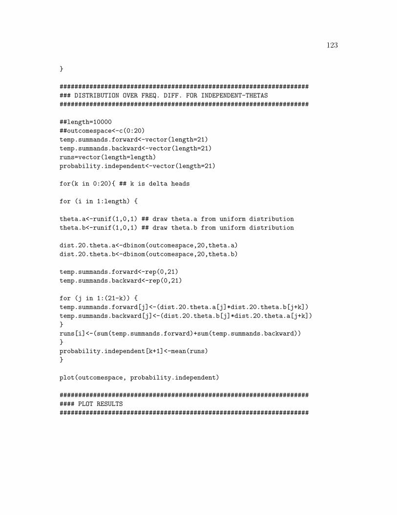
123

}

###################################################################

### DISTRIBUTION OVER FREQ. DIFF. FOR INDEPENDENT-THETAS

###################################################################

##length=10000

##outcomespace<-c(0:20)

temp.summands.forward<-vector(length=21)

temp.summands.backward<-vector(length=21)

runs=vector(length=length)

probability.independent<-vector(length=21)

for(k in 0:20){ ## k is delta heads

for (i in 1:length) {

theta.a<-runif(1,0,1) ## draw theta.a from uniform distribution

theta.b<-runif(1,0,1) ## draw theta.b from uniform distribution

dist.20.theta.a<-dbinom(outcomespace,20,theta.a)

dist.20.theta.b<-dbinom(outcomespace,20,theta.b)

temp.summands.forward<-rep(0,21)

temp.summands.backward<-rep(0,21)

for (j in 1:(21-k)) {

temp.summands.forward[j]<-(dist.20.theta.a[j]*dist.20.theta.b[j+k])

temp.summands.backward[j]<-(dist.20.theta.b[j]*dist.20.theta.a[j+k])

}

runs[i]<-(sum(temp.summands.forward)+sum(temp.summands.backward))

}

probability.independent[k+1]<-mean(runs)

}

plot(outcomespace, probability.independent)

###################################################################

#### PLOT RESULTS

###################################################################

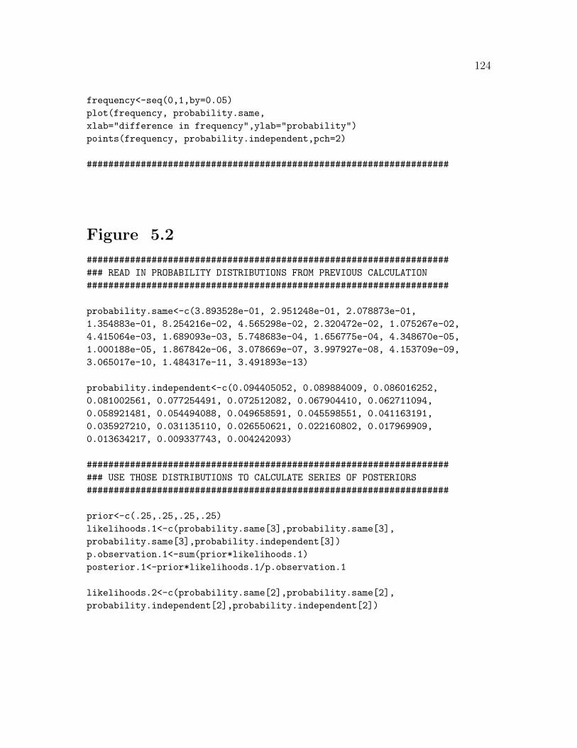
124

frequency<-seq(0,1,by=0.05)

plot(frequency, probability.same,

xlab="difference in frequency",ylab="probability")

points(frequency, probability.independent,pch=2)

###################################################################

Figure 5.2

###################################################################

### READ IN PROBABILITY DISTRIBUTIONS FROM PREVIOUS CALCULATION

###################################################################

probability.same<-c(3.893528e-01, 2.951248e-01, 2.078873e-01,

1.354883e-01, 8.254216e-02, 4.565298e-02, 2.320472e-02, 1.075267e-02,

4.415064e-03, 1.689093e-03, 5.748683e-04, 1.656775e-04, 4.348670e-05,

1.000188e-05, 1.867842e-06, 3.078669e-07, 3.997927e-08, 4.153709e-09,

3.065017e-10, 1.484317e-11, 3.491893e-13)

probability.independent<-c(0.094405052, 0.089884009, 0.086016252,

0.081002561, 0.077254491, 0.072512082, 0.067904410, 0.062711094,

0.058921481, 0.054494088, 0.049658591, 0.045598551, 0.041163191,

0.035927210, 0.031135110, 0.026550621, 0.022160802, 0.017969909,

0.013634217, 0.009337743, 0.004242093)

###################################################################

### USE THOSE DISTRIBUTIONS TO CALCULATE SERIES OF POSTERIORS

###################################################################

prior<-c(.25,.25,.25,.25)

likelihoods.1<-c(probability.same[3],probability.same[3],

probability.same[3],probability.independent[3])

p.observation.1<-sum(prior*likelihoods.1)

posterior.1<-prior*likelihoods.1/p.observation.1

likelihoods.2<-c(probability.same[2],probability.same[2],

probability.independent[2],probability.independent[2])

125

p.observation.2<-sum(posterior.1*likelihoods.2)

posterior.2<-posterior.1*likelihoods.2/p.observation.2

likelihoods.3<-c(probability.same[1],probability.independent[1],

probability.independent[1],probability.independent[1])

p.observation.3<-sum(posterior.2*likelihoods.3)

posterior.3<-posterior.2*likelihoods.3/p.observation.3

###################################################################

### PLOT RESULTS

###################################################################

quartz(width=10,height=12)

par(mfrow=c(2,2))

barplot(prior,ylim=c(0,.75), xlab="hypotheses", ylab="probability",

names.arg=c(1,2,3,4), main="Prior probabilities for hypotheses 1-4")

barplot(posterior.1,ylim=c(0,.75), xlab="hypotheses",

ylab="probability", names.arg=c(1,2,3,4),

main = expression(paste("Posterior probabilities after observing ",

"|",bar(a)-bar(b),"|")) )

barplot(posterior.2,ylim=c(0,.75), xlab="hypotheses",

ylab="probability", names.arg=c(1,2,3,4),

main = expression(paste( , " after subsequently observing ",

"|",bar(a)-bar(c),"|")) )

barplot(posterior.3,ylim=c(0,.75), xlab="hypotheses",

ylab="probability", names.arg=c(1,2,3,4),

main = expression(paste( , " and then after observing ",

"|",bar(a)-bar(d),"|")) )

#######################################################################

Figure 5.3

#################################################################

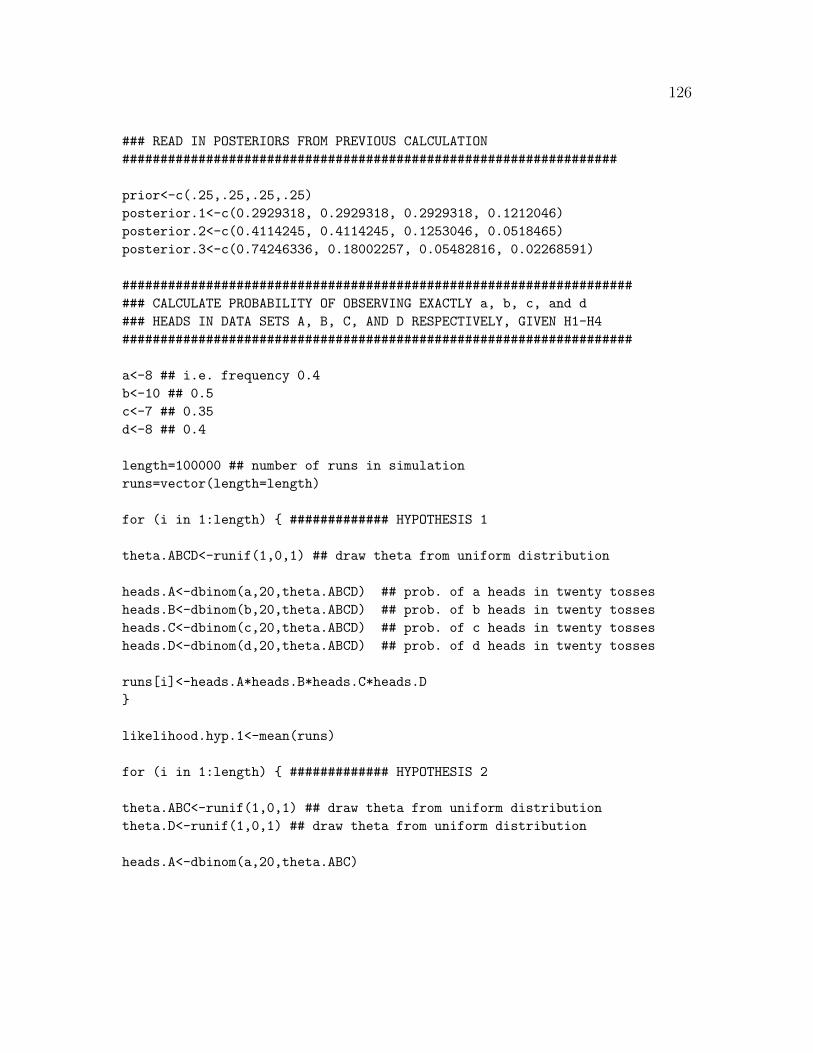
126

### READ IN POSTERIORS FROM PREVIOUS CALCULATION

#################################################################

prior<-c(.25,.25,.25,.25)

posterior.1<-c(0.2929318, 0.2929318, 0.2929318, 0.1212046)

posterior.2<-c(0.4114245, 0.4114245, 0.1253046, 0.0518465)

posterior.3<-c(0.74246336, 0.18002257, 0.05482816, 0.02268591)

###################################################################

### CALCULATE PROBABILITY OF OBSERVING EXACTLY a, b, c, and d

### HEADS IN DATA SETS A, B, C, AND D RESPECTIVELY, GIVEN H1-H4

###################################################################

a<-8 ## i.e. frequency 0.4

b<-10 ## 0.5

c<-7 ## 0.35

d<-8 ## 0.4

length=100000 ## number of runs in simulation

runs=vector(length=length)

for (i in 1:length) { ############# HYPOTHESIS 1

theta.ABCD<-runif(1,0,1) ## draw theta from uniform distribution

heads.A<-dbinom(a,20,theta.ABCD) ## prob. of a heads in twenty tosses

heads.B<-dbinom(b,20,theta.ABCD) ## prob. of b heads in twenty tosses

heads.C<-dbinom(c,20,theta.ABCD) ## prob. of c heads in twenty tosses

heads.D<-dbinom(d,20,theta.ABCD) ## prob. of d heads in twenty tosses

runs[i]<-heads.A*heads.B*heads.C*heads.D

}

likelihood.hyp.1<-mean(runs)

for (i in 1:length) { ############# HYPOTHESIS 2

theta.ABC<-runif(1,0,1) ## draw theta from uniform distribution

theta.D<-runif(1,0,1) ## draw theta from uniform distribution

heads.A<-dbinom(a,20,theta.ABC)

127

heads.B<-dbinom(b,20,theta.ABC)

heads.C<-dbinom(c,20,theta.ABC)

heads.D<-dbinom(d,20,theta.D)

runs[i]<-heads.A*heads.B*heads.C*heads.D

}

likelihood.hyp.2<-mean(runs)

for (i in 1:length) { ############# HYPOTHESIS 3

theta.AB<-runif(1,0,1)

theta.C<-runif(1,0,1)

theta.D<-runif(1,0,1)

heads.A<-dbinom(a,20,theta.AB)

heads.B<-dbinom(b,20,theta.AB)

heads.C<-dbinom(c,20,theta.C)

heads.D<-dbinom(d,20,theta.D)

runs[i]<-heads.A*heads.B*heads.C*heads.D

}

likelihood.hyp.3<-mean(runs)

for (i in 1:length) { ############# HYPOTHESIS 4

theta.A<-runif(1,0,1)

theta.B<-runif(1,0,1)

theta.C<-runif(1,0,1)

theta.D<-runif(1,0,1)

heads.A<-dbinom(a,20,theta.A)

heads.B<-dbinom(b,20,theta.B)

heads.C<-dbinom(c,20,theta.C)

heads.D<-dbinom(d,20,theta.D)

runs[i]<-heads.A*heads.B*heads.C*heads.D

}

likelihood.hyp.4<-mean(runs)

128

#################################################################

### USE THOSE LIKELIHOODS TO CALCULATE POSTERIORS

### AFTER OBSERVING NUMBERS OF HEADS: a, b, c, and d

#################################################################

prior<-c(.25,.25,.25,.25)

likelihoods.fc<-c(likelihood.hyp.1,likelihood.hyp.2,

likelihood.hyp.3,likelihood.hyp.4)

p.observation.fc<-sum(.25*likelihoods)

posterior.fc<-prior*likelihoods.fc/p.observation.fc

#################################################################

### CALCULATE LIKELIHOODS FOR OBSERVING |a40-b40|

#################################################################

k<-4 ## k is delta heads

length=100000 ## number of runs in simulation

outcomespace<-c(0:40) ##outcome space for 40 tosses

temp.summands<-vector(length=41)

temp.summands.backward<-vector(length=41)

runs=vector(length=length)

for (i in 1:length) { ## same-theta hypotheses

theta.AB<-runif(1,0,1)

dist.40.theta.AB<-dbinom(outcomespace,40,theta.AB)

temp.summands<-rep(0,41)

for (j in 1:(41-k)) {

temp.summands[j]<-(dist.40.theta.AB[j]*dist.40.theta.AB[j+k])

runs[i]<-2*(sum(temp.summands))

}

}

likelihood40.same.theta<-mean(runs)

for (i in 1:length) { ## independent-theta hypotheses

theta.A<-runif(1,0,1)

129

theta.B<-runif(1,0,1)

dist.40.theta.A<-dbinom(outcomespace,40,theta.A)

dist.40.theta.B<-dbinom(outcomespace,40,theta.B)

temp.summands<-rep(0,41)

for (j in 1:(41-k)) {

temp.summands[j]<-(dist.40.theta.A[j]*dist.40.theta.B[j+k])

temp.summands.backward[j]<-(dist.40.theta.B[j]*dist.40.theta.A[j+k])

runs[i]<-sum(temp.summands)+sum(temp.summands.backward)

}

}

likelihood40.ind.theta<-mean(runs)

likelihoods40<-c(likelihood40.same.theta, likelihood40.same.theta,

likelihood40.same.theta, likelihood40.ind.theta)

#################################################################

### USE THOSE LIKELIHOODS TO CALCULATE POSTERIORS

#################################################################

p.observation40<-sum(prior*likelihoods40)

posterior40<-prior*likelihoods40/p.observation40

###################################################################

### CALCULATE PROBABILITY OF OBSERVING a40 and b40, GIVEN H1-H4

###################################################################

a<-16 ## i.e., frequency=0.4

b<-20 ## i.e., frequency=0.5

length=100000 ## number of runs in simulation

runs=vector(length=length)

for (i in 1:length) { ## for same theta hypotheses

theta.A<-runif(1,0,1)

heads.A<-dbinom(a,40,theta.A)

heads.B<-dbinom(b,40,theta.A)

runs[i]<-heads.A*heads.B

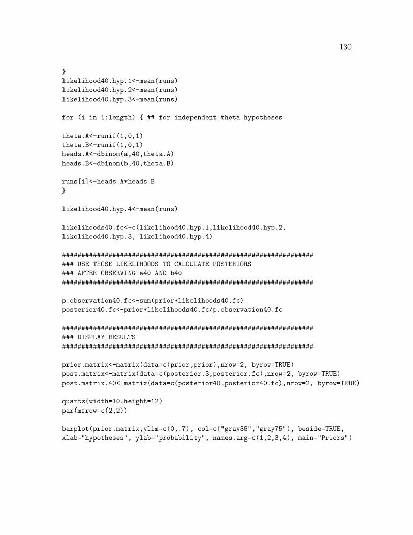
130

}

likelihood40.hyp.1<-mean(runs)

likelihood40.hyp.2<-mean(runs)

likelihood40.hyp.3<-mean(runs)

for (i in 1:length) { ## for independent theta hypotheses

theta.A<-runif(1,0,1)

theta.B<-runif(1,0,1)

heads.A<-dbinom(a,40,theta.A)

heads.B<-dbinom(b,40,theta.B)

runs[i]<-heads.A*heads.B

}

likelihood40.hyp.4<-mean(runs)

likelihoods40.fc<-c(likelihood40.hyp.1,likelihood40.hyp.2,

likelihood40.hyp.3, likelihood40.hyp.4)

#################################################################

### USE THOSE LIKELIHOODS TO CALCULATE POSTERIORS

### AFTER OBSERVING a40 AND b40

#################################################################

p.observation40.fc<-sum(prior*likelihoods40.fc)

posterior40.fc<-prior*likelihoods40.fc/p.observation40.fc

#################################################################

### DISPLAY RESULTS

#################################################################

prior.matrix<-matrix(data=c(prior,prior),nrow=2, byrow=TRUE)

post.matrix<-matrix(data=c(posterior.3,posterior.fc),nrow=2, byrow=TRUE)

post.matrix.40<-matrix(data=c(posterior40,posterior40.fc),nrow=2, byrow=TRUE)

quartz(width=10,height=12)

par(mfrow=c(2,2))

barplot(prior.matrix,ylim=c(0,.7), col=c("gray35","gray75"), beside=TRUE,

xlab="hypotheses", ylab="probability", names.arg=c(1,2,3,4), main="Priors")

131

barplot(post.matrix,ylim=c(0,.7), col=c("gray35","gray75"),

beside=TRUE, xlab="hypotheses", ylab="probability",

names.arg=c(1,2,3,4), main = "Posteriors (four \"kinds\")",

legend=c("frequency differences","full frequencies") )

barplot(prior.matrix,ylim=c(0,.7), col=c("gray35","gray75"), beside=TRUE,

xlab="hypotheses", ylab="probability", names.arg=c(1,2,3,4), main="Priors")

barplot(post.matrix.40,ylim=c(0,.7), col=c("gray35","gray75"),

beside=TRUE, xlab="hypotheses", ylab="probability",

names.arg=c(1,2,3,4), main = "Posteriors (two \"kinds\")",

legend=c("frequency differences","full frequencies") )

#################################################################

132

Bibliography

Boring, E. (1954). The nature and history of experimental control, The Americanjournal of psychology 67(4): 573–589.

Bovens, L. and Hartmann, S. (2003). Bayesian Epistemology, Oxford UniversityPress.

Bowler, P. (1989). Evolution: The history of an idea, University of California Press.

Darwin, C. (1859/2003). On the Origin of Species: A Facsimile of the First Edition,Harvard University Press.

Earman, J. (1992). Bayes or Bust? A critical examination of Bayesian confirmationtheory, MIT press.

Edwards, A. W. F. (1984). Likelihood, Cambridge University Press.

Fitelson, B. (2001). A Bayesian account of independent evidence with applications,Philosophy of Science 68(3): S123–S140.

Fitelson, B. (2011). Favoring, likelihoodism, and Bayesianism, Philosophy and Phe-nomenological Research 83(3): 666–672.

Forster, M. (1988). Unification, explanation, and the composition of causes in New-tonian mechanics, Studies In History and Philosophy of Science Part A 19(1): 55–101.

Forster, M. (2011). The debate between Whewell and Mill on the nature of scientificinduction, in S. Gabbay, D. Hartmann and J. Woods (eds), Inductive Logic, Vol. 10of Handbook of the history of logic, North Holland, pp. 93–115.

Forster, M. R. (2007). A philosopher’s guide to empirical success, Philosophy ofScience 74(5): 588–600.

133

Forster, M. and Sober, E. (2011). AIC scores as evidence–a Bayesian interpretation,in P. S. Bandyopadhyay and M. Forster (eds), Philosophy of Statistics, Handbookof the Philosophy of Science, North Holland.

Funk, D. J., Helbling, L., Wernegreen, J. J. and Moran, N. A. (2000). Intraspecificphylogenetic congruence among multiple symbiont genomes, Proceedings of theRoyal Society of London. Series B: Biological Sciences 267(1461): 2517–2521.

Ghiselin, M. T. (1969). The triumph of the Darwinian method, University of Cali-fornia Press.

Hacking, I. (1965). The Logic of Statistical Inference, Cambridge University Press.

Hacking, I. (1985). Do we see through a microscope?, in P. M. Churchland and C. A.Hooker (eds), Images of science: Essays on realism and empiricism, with a replyfrom Bas C. van Fraassen, University of Chicago Press.

Harper, W. (2007). Newton’s methodology and Mercury’s perihelion before and afterEinstein, Philosophy of Science 74(5): 932–942.

Hempel, C. (1966). Philosophy of Natural Science, Prentice-Hall.

Hodge, M. J. S. (1991). Discussion note: Darwin, Whewell, and natural selection,Biology and Philosophy 6(4): 457–460.

Howson, C. and Urbach, P. (1993). Scientific reasoning, the Bayesian approach, 2ndedn, Open Court Publishing.

Huelsenbeck, J. P., Bull, J. J. and Cunningham, C. W. (1996). Combining data inphylogenetic analysis, Trends in Ecology & Evolution 11(4): 152–158.

Kitcher, P. (1993). The Advancement of Science: Science Without Legend, ObjectivityWithout Illusions, Oxford University Press, USA, chapter 2.

Kitcher, P. (2003). In Mendel’s Mirror: Philosophical Reflections on Biology, OxfordUniversity Press, chapter 3.

Koolage, J. (2008). Realism and the agreement of measurements, PhD thesis, Uni-versity of Wisconsin–Madison.

Larson, E. J. (2004). Evolution: The Remarkable History of a Scientific Theory,Random House Digital, Inc.

134

Lloyd, E. A. (1983). The nature of Darwin’s support for the theory of naturalselection, Philosophy of science 50(1): 112–129.

Myrvold, W. (1996). Bayesianism and diverse evidence: A reply to Andrew Wayne,Philosophy of Science pp. 661–665.

Nelson, G. (1978). From Candolle to Croizat: comments on the history of biogeog-raphy, Journal of the History of Biology 11(2): 269–305.

Norton, J. (2000). How we know about electrons, in R. Nola and H. Sankey (eds), Af-ter Popper, Kuhn and Feyerabend: Recent Issues in Theories of Scientific Method,Kluwer Academic Publishers.

O’Hara, R. J. (1991). Representations of the natural system in the nineteenth cen-tury, Biology and Philosophy 6(2): 255–274.

Penny, D., Foulds, L. and Hendy, M. (1982). Testing the theory of evolution bycomparing phylogenetic trees constructed from five different protein sequences,Nature 297: 197–200.

Penny, D. and Hendy, M. (1985). The use of tree comparison metrics, SystematicZoology pp. 75–82.

Recker, D. A. (1987). Causal efficacy: The structure of Darwin’s argument strategyin the “Origin of Species”, Philosophy of science 54(2): 147–175.

Robinson, D. and Foulds, L. R. (1981). Comparison of phylogenetic trees, Mathe-matical Biosciences 53(1): 131–147.

Royall, R. M. (1997). Statistical Evidence: A Likelihood Paradigm, Chapman andHall.

Ruse, M. (1975). Darwin’s debt to philosophy: An examination of the influence of thephilosophical ideas of john fw herschel and William Whewell on the development ofCharles Darwin’s theory of evolution, Studies in history and philosophy of science6(2): 159.

Salmon, W. (1984). Scientific Explanation and the Causal Structure of the World,Princeton University Press.

Schlosshauer, M. and Wheeler, G. (2011). Focused correlation, confirmation, andthe jigsaw puzzle of variable evidence, Philosophy of Science 78(3): 376–392.

135

Sober, E. (1989). Independent evidence about a common cause, Philosophy of Science56(2): pp. 275–287.

Sober, E. (1999). Modus Darwin, Biology and Philosophy 14(2): 253–278.

Sober, E. (2008). Evidence and Evolution: The Logic Behind the Science, CambridgeUniversity Press.

Sober, E. (2011). Did Darwin Write the Origin Backwards?: Philosophical Essayson Darwin’s Theory, Prometheus Books.

Sober, E. and Steel, M. (2002). Testing the hypothesis of common ancestry, Journalof Theoretical Biology 218(4): 395–408.

Steel, D. (1996). Bayesianism and the value of diverse evidence, Philosophy of Sciencepp. 666–674.

Thagard, P. (1977). Darwin and Whewell, Studies In History and Philosophy ofScience 8(4): 353–356.

Thagard, P. R. (1978). The best explanation: Criteria for theory choice, The Journalof Philosophy 75(2): 76–92.

Waters, C. K. (2003). The arguments in the Origin of Species, in G. Radick (ed.),The Cambridge Companion to Darwin, Cambridge Univ Press, chapter 5, p. 116.

Wayne, A. (1995). Bayesianism and diverse evidence, Philosoph of Science62(1): 111–121.

Wheeler, G. (2009). Focused correlation and confirmation, The British Journal forthe Philosophy of Science 60(1): 79–100.

Wheeler, G. and Scheines, R. (2011). Causation, association and confirmation, Ex-planation, Prediction, and Confirmation pp. 37–51.

Whewell, W. (1858/1989a). Novum organon renovatum, in R. E. Butts (ed.), WilliamWhewell: Theory of Scientific Method, Hackett.

Whewell, W. (1860/1989b). On the philosophy of discovery: Chapters historicaland critical, in R. E. Butts (ed.), William Whewell: Theory of Scientific Method,Hackett.

136

Wiley, E. O. (1988). Vicariance biogeography, Annual Review of Ecology and Sys-tematics 19: 513–542.

Winsor, M. (2009). Taxonomy was the foundation of Darwin’s evolution, Taxon58(1): 43–49.