district court 13 - moritzlaw.osu.edu · - 2 - 4. the following chart contains the number of seats...

IN THE UNITED STATES DISTRICT COURT

FOR THE WESTERN DISTRICT OF WISCONSIN

WILLIAM WHITFORD, et al.,

Plaintiffs,

v. Case No. 15-CV-421-bbc

GERALD NICHOL, et al.,

Defendants.

DEFENDANTS’ PROPOSED FINDINGS OF FACT

______________________________________________________________________________

The defendants, Gerald Nichol, et al., by their attorneys, Wisconsin Attorney

General Brad D. Schimel and Assistant Attorneys General Brian P. Keenan and

Anthony D. Russomanno, and pursuant to the Court’s October 15, 2015,

Preliminary Pretrial Conference Order, offer the following findings of fact the

defendants request the Court to find after trial:

HISTORY OF ELECTIONS IN WISCONSIN

1. The Government Accountability Board’s official election results are

authoritative for Wisconsin elections dating back to the year 2000.

2. For elections in years prior to 2000, the Wisconsin Blue Book’s election

results are authoritative.

3. The City of Milwaukee Election Commission maintains election results

dating back to 1997 on its website. These results are authoritative for election

results in the City of Milwaukee.

Case: 3:15-cv-00421-bbc Document #: 124 Filed: 05/09/16 of 58

- 2 -

4. The following chart contains the number of seats won by Democratic,

Republican and Independent candidates in the November general elections from

1972 to 2014. The party with the majority is listed in bold.

Year Democrat Republican Independent

1972 62 37

1974 63 36

1976 66 33

1978 60 39

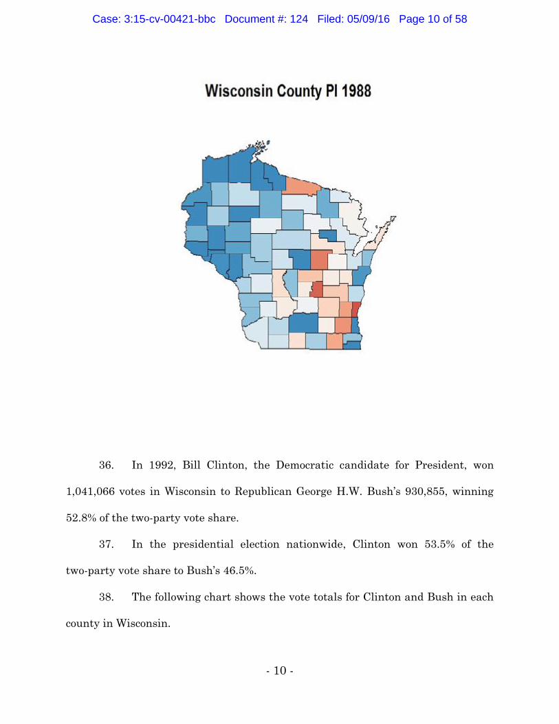
1980 59 40

1982 59 40

1984 52 47

1986 54 45

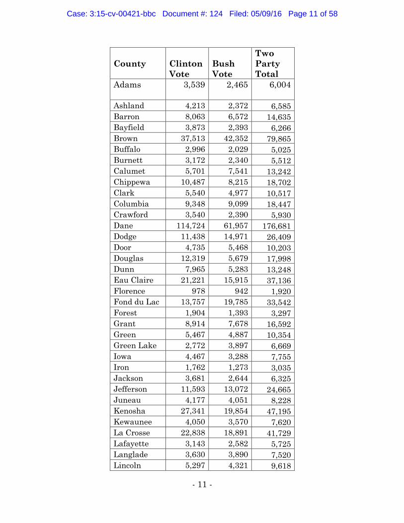
1988 56 43

1990 58 41

1992 52 47

1994 48 51

1996 47 52

1998 44 55

2000 43 56

2002 41 58

2004 39 60

2006 47 52

2008 52 46 1

2010 38 60 1

2012 39 60

2014 36 63

5. The Democrats won a majority of seats in the Wisconsin Assembly in

each general election from 1972 through 1994.

6. The Republicans won a majority of seats in the Wisconsin Assembly in

each general election from 1994 through 2014, with the exception of the 2008

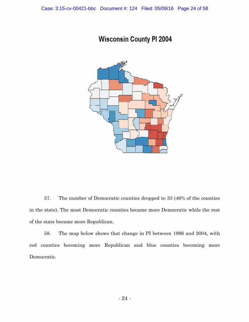
election.


- 3 -

7. The Assembly map in place for the 1972, 1974, 1976, 1978 and 1980

plans was enacted by the Democratic Assembly and Republican Senate and signed

by a Democratic Governor.

8. The Assembly map in place for the 1982 election was put in place by

the federal court in Wisconsin State AFL-CIO v. Elections Bd., 543 F. Supp. 630

(E.D. Wis. 1982).

9. The Assembly map in place for the 1982 election was amended and

enacted by the Democratic Assembly and Democratic Senate and signed by a

Democratic Governor and was then in place for the 1984, 1986, 1988 and 1990

elections.


elections was drawn by the federal court in Prosser v. Elections Board, 793 F. Supp.

859 (W.D. Wis. 1992).


elections was drawn by the federal court in Baumgart v. Wendelberger,

No. 01–C–0121, 2002 WL 34127471, at *1 (E.D. Wis. May 30, 2002), amended, 2002

WL 34127473 (E.D. Wis. July 11, 2002).

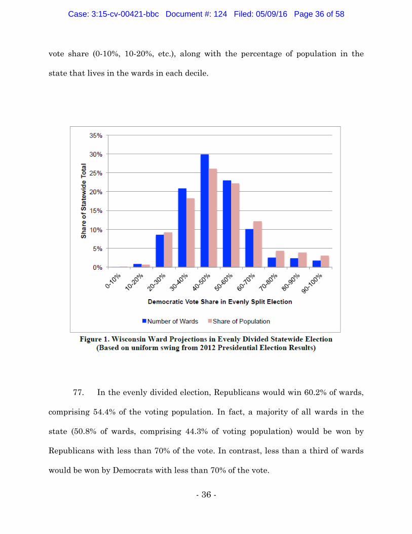
12. Professor Jackman analyzed each Wisconsin Assembly election since

1972 and found that Wisconsin’s EG has ranged from a high (most favorable to

Democrats) of +2.48% in 1994 to a low (most favorable to Republicans) of –13.31%

in 2012.


- 4 -

13. Disregarding results from the current plan, the lowest EG was

–11.83% in 2006.

14. The most favorable EG towards Democrats notably occurred in 1994

when the Republicans gained control of the Assembly for the first time since the

1968 election.

15. Professor Jackman finds that “Wisconsin has recorded an unbroken

run of negative EG estimates from 1998 to 2014.”

16. The last positive EG that Professor Jackman found in Wisconsin was

the 2.48% from 1994.

17. With respect to the 2002 Plan, Professor Jackman calculated an

average efficiency gap of –7.6%, with –4.0% as the most favorable year to Democrats

and –11.8% as the most favorable year to Republicans.

18. In 1992, the Democrats’ seat share rounded to the nearest .25% was

52.5%. Given that Professor Jackman calculates an EG of –2%, the Democratic vote

share was 52.25% because the implied seat share if the efficiency gap was zero is

54.5%

19. In 1994, the Democrats’ seat share rounded to the nearest 0.25% was

48.5%. Given that Professor Jackman calculates an EG of +2%, the Democratic vote


46.5%.


47.5%. Given that Professor Jackman calculates an EG of 0%, the Democratic vote


- 5 -


47.5%.


44.5%. Given that Professor Jackman calculates an EG of –7.5%, the Democratic

vote share was 51% because the implied seat share if the efficiency gap was zero is

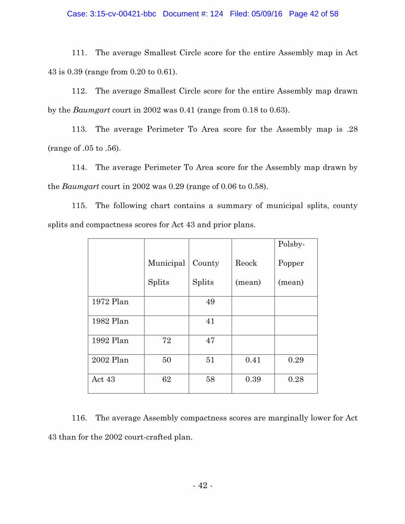
52%.


43.5%. Given that Professor Jackman calculates an EG of –6%, the Democratic vote


49.5%.


41.5%. Given that Professor Jackman calculates an EG of –7.5%, the Democratic

vote share was 49.5% because the implied seat share if the efficiency gap was zero is

49%.


40%. Given that Professor Jackman calculates an EG of –10%, the Democratic vote

share was 50% because the implied seat share if the efficiency gap was zero is 50%.


47.5%. Given that Professor Jackman calculates an EG of –12%, the Democratic

vote share was 54.75% because the implied seat share if the efficiency gap was zero

is 59.5%.


- 6 -



share was 54% because the implied seat share if the efficiency gap was zero is 58%.




43%.

28. In 2012, Professor Jackman calculates that the Democrats’ vote share

was 51.4%. This yields an implied seat share of 52.8% if the efficiency gap was zero.

The Democrats’ actual seat share was 39.4%, yielding an efficiency gap of –13.4%.

29. In 2014, Professor Jackman calculates that the Democrats’ vote share

was 48.0%. This yields an implied seat share of 46.0% if the efficiency gap was zero.

Their actual seat share was 36.4%, which yields an efficiency gap of –9.6%.

30. In 1988, Michael Dukakis, the Democratic candidate for President,

won 1,126,794 votes in Wisconsin to Republican George H.W. Bush’s 1,047,499

votes, winning 51.8% of the two-party vote.

31. In the presidential election nationwide, George H.W. Bush won 53.9%

of the two-party vote and Dukakis won 46.1%.

32. The following chart shows the vote totals for Dukakis and Bush in each

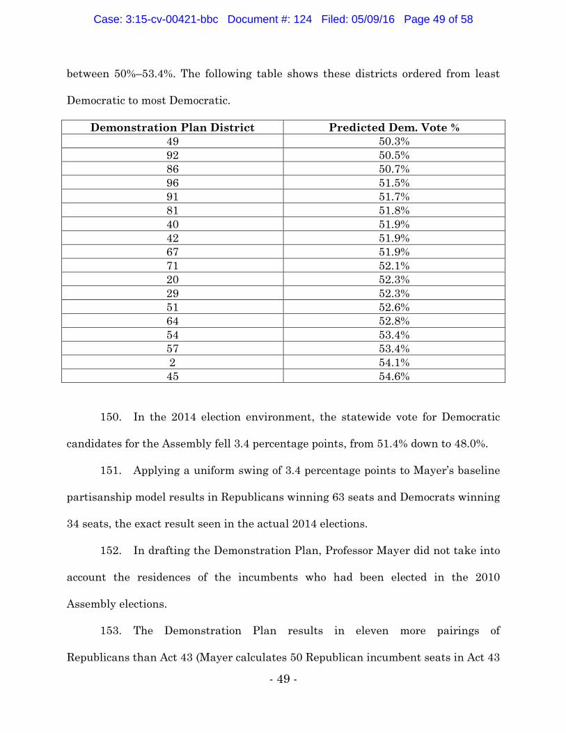
county in Wisconsin.

County Dukakis

Vote

Bush

Vote

Two

Party

Total

Adams 3,598 3,258 6,856


- 7 -

County Dukakis

Vote

Bush

Vote

Two

Party

Total

Ashland 4,526 2,926 7,452

Barron 8,951 8,527 17,478

Bayfield 4,323 3,095 7,418

Brown 41,788 43,625 85,413

Buffalo 3,481 2,783 6,264

Burnett 3,537 2,884 6,421

Calumet 6,481 8,107 14,588

Chippewa 11,447 9,757 21,204

Clark 6,642 6,296 12,938

Columbia 9,132 10,475 19,607

Crawford 3,608 3,238 6,846

Dane 105,414 69,143 174,557

Dodge 12,663 17,003 29,666

Door 5,425 6,907 12,332

Douglas 13,907 6,440 20,347

Dunn 9,205 7,273 16,478

Eau Claire 21,150 17,664 38,814

Florence 1,018 1,106 2,124

Fond du Lac 15,887 21,985 37,872

Forest 2,142 1,845 3,987

Grant 9,421 10,049 19,470

Green 5,153 6,636 11,789

Green Lake 3,033 5,205 8,238

Iowa 4,268 4,240 8,508

Iron 2,090 1,599 3,689

Jackson 3,924 3,555 7,479

Jefferson 11,816 14,309 26,125

Juneau 3,734 4,869 8,603

Kenosha 30,089 21,661 51,750

Kewaunee 4,786 4,330 9,116

La Crosse 22,204 21,548 43,752

Lafayette 3,521 3,665 7,186

Langlade 4,254 4,884 9,138

Lincoln 5,819 5,257 11,076

Manitowoc 19,680 16,020 35,700

Marathon 24,658 24,482 49,140


- 8 -

County Dukakis

Vote

Bush

Vote

Two

Party

Total

Marinette 8,030 9,637 17,667

Marquette 2,463 3,059 5,522

Menominee 1,028 381 1,409

Milwaukee 268,287 168,363 436,650

Monroe 6,437 7,073 13,510

Oconto 6,549 7,084 13,633

Oneida 7,414 8,130 15,544

Outagamie 27,771 33,113 60,884

Ozaukee 12,661 22,899 35,560

Pepin 1,906 1,311 3,217

Pierce 8,659 6,045 14,704

Polk 8,981 6,866 15,847

Portage 16,317 12,057 28,374

Price 3,987 3,450 7,437

Racine 39,631 36,342 75,973

Richland 3,643 4,026 7,669

Rock 29,576 28,178 57,754

Rusk 3,888 3,063 6,951

St. Croix 11,392 9,960 21,352

Sauk 8,324 10,225 18,549

Sawyer 3,231 3,260 6,491

Shawano 6,587 8,362 14,949

Sheboygan 23,429 23,471 46,900

Taylor 3,785 4,254 8,039

Trempealeau 6,212 4,902 11,114

Vernon 5,754 5,226 10,980

Vilas 3,781 5,842 9,623

Walworth 12,203 18,259 30,462

Washburn 3,393 3,074 6,467

Washington 15,907 24,328 40,235

Waukesha 57,598 90,467 148,065

Waupaca 7,078 11,559 18,637

Waushara 3,535 4,953 8,488

Winnebago 28,508 35,085 63,593


- 9 -

County Dukakis

Vote

Bush

Vote

Two

Party

Total

Wood 16,074 16,549 32,623

1,126,794 1,047,499 2,174,293

33. The following chart shows the vote totals and two-party vote

percentages for Dukakis and Bush in Dane, Milwaukee and Rock Counties.

County Dukakis Vote Bush Vote Two Party Total

Dane 105,414 (60.39%) 69,143 (39.61%) 174,557

Milwaukee 268,287 (61.44%) 168,363 (38.56%) 436,650

Rock 29,576 (51.21%) 28,178 (48.79%) 57,754

34. In 1988, the Democratic Party in Wisconsin had a broad geographic

reach. It was strongest on the Menominee Indian Reservation (Partisan Index of

26.86), as is the case today. The other four most Democratic counties were Douglas

(22.47 PI), Milwaukee (15.34 PI), Ashland (14.63) and Dane (14.3). Seventy-one

percent of counties had Democratic leans, and the Democratic Party covered the

entire Western portion of the State, particularly in the northwest. Republicans were

relegated to suburban and rural counties in the southeast and east-central portions

of the State.

35. The following map shows the PIs of each county in Wisconsin in 1988,

with blue shading for counties with Democratic leans and red shading for counties

with Republican leans, with darker shading for stronger leans.


- 10 -

36. In 1992, Bill Clinton, the Democratic candidate for President, won

1,041,066 votes in Wisconsin to Republican George H.W. Bush’s 930,855, winning

52.8% of the two-party vote share.

37. In the presidential election nationwide, Clinton won 53.5% of the

two-party vote share to Bush’s 46.5%.

38. The following chart shows the vote totals for Clinton and Bush in each



- 11 -

County Clinton

Vote

Bush

Vote

Two

Party

Total

Adams 3,539 2,465 6,004

Ashland 4,213 2,372 6,585

Barron 8,063 6,572 14,635

Bayfield 3,873 2,393 6,266

Brown 37,513 42,352 79,865

Buffalo 2,996 2,029 5,025

Burnett 3,172 2,340 5,512

Calumet 5,701 7,541 13,242

Chippewa 10,487 8,215 18,702

Clark 5,540 4,977 10,517

Columbia 9,348 9,099 18,447

Crawford 3,540 2,390 5,930

Dane 114,724 61,957 176,681

Dodge 11,438 14,971 26,409

Door 4,735 5,468 10,203

Douglas 12,319 5,679 17,998

Dunn 7,965 5,283 13,248

Eau Claire 21,221 15,915 37,136

Florence 978 942 1,920

Fond du Lac 13,757 19,785 33,542

Forest 1,904 1,393 3,297

Grant 8,914 7,678 16,592

Green 5,467 4,887 10,354

Green Lake 2,772 3,897 6,669

Iowa 4,467 3,288 7,755

Iron 1,762 1,273 3,035

Jackson 3,681 2,644 6,325

Jefferson 11,593 13,072 24,665

Juneau 4,177 4,051 8,228

Kenosha 27,341 19,854 47,195

Kewaunee 4,050 3,570 7,620

La Crosse 22,838 18,891 41,729

Lafayette 3,143 2,582 5,725

Langlade 3,630 3,890 7,520

Lincoln 5,297 4,321 9,618


- 12 -

County Clinton

Vote

Bush

Vote

Two

Party

Total

Manitowoc 15,903 14,008 29,911

Marathon 21,482 20,948 42,430

Marinette 7,626 7,984 15,610

Marquette 2,533 2,322 4,855

Menominee 691 244 935

Milwaukee 235,521 151,314 386,835

Monroe 6,427 6,118 12,545

Oconto 5,898 5,720 11,618

Oneida 7,160 6,725 13,885

Outagamie 23,735 30,370 54,105

Ozaukee 11,879 22,805 34,684

Pepin 1,673 1,098 2,771

Pierce 7,824 4,844 12,668

Polk 7,746 5,446 13,192

Portage 15,553 10,914 26,467

Price 3,575 2,654 6,229

Racine 34,875 32,310 67,185

Richland 3,458 3,144 6,602

Rock 31,154 21,942 53,096

Rusk 3376 2,430 3,376

St. Croix 10281 8,114 10,281

Sauk 9128 8,886 9,128

Sawyer 2796 2,658 2,796

Shawano 6,062 7,253 13,315

Sheboygan 20,568 22,526 43,094

Taylor 3,305 3,415 6,720

Trempealeau 6,218 3,577 9,795

Vernon 5,673 4,072 9,745

Vilas 3,764 4,616 8,380

Walworth 11,825 15,727 27,552

Washburn 3,080 2,586 5,666

Washington 13,339 22,739 36,078

Waukesha 50,270 91,461 141,731

Waupaca 6,666 10,252 16,918


- 13 -

County Clinton

Vote

Bush

Vote

Two

Party

Total

Waushara 3,402 4,045 7,447

Winnebago 27,234 33,709 60,943

Wood 13,208 13,843 27,051

1,041,066 930,855 1,971,921


percentages for Clinton and Bush in Dane, Milwaukee and Rock Counties.

County Clinton Vote Bush Vote Two Party Total

Dane 114,724 (64.93%) 61,957 (35.07%) 176,681

Milwaukee 235,521 (60.88%) 151,314 (39.12%) 386,835

Rock 31,154 (58.67%) 21,942 (41.33%) 53,096

40. In 1996, Bill Clinton, the Democratic candidate for President, won

1,071,971 votes in Wisconsin to Republican Bob Dole’s 845,029 votes, winning 55.9%

of the two-party vote share.

41. In the presidential election nationwide, Clinton won 54.7% of the

two-party vote to Dole’s 45.3%.

42. The following chart shows the vote totals for Clinton and Dole in each


County Clinton

Vote

Dole

Vote

Two

Party

Total

Adams 4,119 2,450 6,569

Ashland 3,808 1,863 5,671

Barron 8,025 6,158 14,183


- 14 -

County Clinton

Vote

Dole

Vote

Two

Party

Total

Bayfield 3,895 2,250 6,145

Brown 42,823 38,563 81,386

Buffalo 2,681 1,800 4,481

Burnett 3,625 2,452 6,077

Calumet 6,940 7,049 13,989

Chippewa 9,647 7,520 17,167

Clark 5,540 4,622 10,162

Columbia 10,336 8,377 18,713

Crawford 3,658 2,149 5,807

Dane 109,347 59,487 168,834

Dodge 12,625 12,890 25,515

Door 5,590 4,948 10,538

Douglas 10,976 5,167 16,143

Dunn 7,536 4,917 12,453

Eau Claire 20,298 13,900 34,198

Florence 869 927 1,796

Fond du Lac 15,542 16,488 32,030

Forest 2,092 1,166 3,258

Grant 9,203 7,021 16,224

Green 6,136 4,697 10,833

Green Lake 3,152 3,565 6,717

Iowa 4,690 2,866 7,556

Iron 1,725 1,260 2,985

Jackson 3,705 2,262 5,967

Jefferson 13,188 12,681 25,869

Juneau 4,331 3,226 7,557

Kenosha 27,964 18,296 46,260

Kewaunee 4,311 3,431 7,742

La Crosse 23,647 16,482 40,129

Lafayette 3,261 2,172 5,433

Langlade 4,074 3,206 7,280

Lincoln 6,166 4,076 10,242

Manitowoc 16,750 13,239 29,989

Marathon 24,012 19,874 43,886

Marinette 8,413 7,231 15,644

Marquette 2,859 2,208 5,067


- 15 -

County Clinton

Vote

Dole

Vote

Two

Party

Total

Menominee 992 230 1,222

Milwaukee 216,620 119,407 336,027

Monroe 6,924 5,299 12,223

Oconto 6,723 5,389 12,112

Oneida 7,619 6,339 13,958

Outagamie 28,815 27,758 56,573

Ozaukee 13,269 22,078 35,347

Pepin 1,585 1,007 2,592

Pierce 7,970 4,599 12,569

Polk 8,334 5,387 13,721

Portage 15,901 9,631 25,532

Price 3,523 2,545 6,068

Racine 38,567 30,107 68,674

Richland 3,502 2,642 6,144

Rock 32,450 20,096 52,546

Rusk 2941 2,219 2,941

St. Croix 11384 8,253 11,384

Sauk 9889 7,448 9,889

Sawyer 2773 2,603 2,773

Shawano 6,850 6,396 13,246

Sheboygan 22,022 20,067 42,089

Taylor 3,253 3,108 6,361

Trempealeau 5,848 3,035 8,883

Vernon 5,572 3,796 9,368

Vilas 4,226 4,496 8,722

Walworth 13,283 15,099 28,382

Washburn 3,231 2,703 5,934

Washington 17,154 25,829 42,983

Waukesha 57,354 91,729 149,083

Waupaca 7,800 8,679 16,479

Waushara 3,824 3,573 7,397

Winnebago 29,564 27,880 57,444

Wood 14,650 12,666 27,316

1,071,971 845,029 1,917,000


- 16 -

43. Bill Clinton won Milwaukee, Dane and Rock Counties with 64% of the

two–party vote and carried the rest of the state with 52% of the vote, a difference of

twelve percentage points.

44. In 1996, forty-five counties (62.5%) had Democratic leans.

45. Below is a map showing the PIs of Wisconsin’s counties in 1996.


- 17 -


percentages for Clinton and Dole in Dane, Milwaukee and Rock Counties.

County Clinton Vote Dole Vote Two Party Total

Dane 109,347 (64.77%) 59,487 (35.23%) 168,834

Milwaukee 216,620 (64.47%) 119,407 (35.53%) 336,027

Rock 32,450 (61.75%) 20,096 (38.25%) 52,246

47. In 2000, Albert Gore, the Democratic candidate for President, won

1,242,987 votes in Wisconsin to Republican George W. Bush’s 1,237,279 votes,

winning 50.1% of the two-party vote.

48. In the presidential election nationwide, Gore won 50.27% of the

two-party vote to Bush’s 49.73%.

49. The following chart shows the vote totals for Gore and Bush in each

county in Wisconsin, as well as a subtotal for votes in the City of Milwaukee.

County Gore

Vote

Bush

Vote

Two

Party

Total

Adams 4,826 3,920 8,746

Ashland 4,356 3,038 7,394

Barron 8,928 9,848 18,776

Bayfield 4,427 3,266 7,693

Brown 49,096 54,258 103,354

Buffalo 3,237 3,038 6,275

Burnett 3,626 3,967 7,593

Calumet 8,202 10,837 19,039

Chippewa 12,102 12,835 24,937

Clark 5,931 7,461 13,392

Columbia 12,636 11,987 24,623


- 18 -

County Gore

Vote

Bush

Vote

Two

Party

Total

Crawford 4,005 3,024 7,029

Dane 142,317 75,790 218,107

Dodge 14,580 21,684 36,264

Door 6,560 7,810 14,370

Douglas 13,593 6,930 20,523

Dunn 9,172 8,911 18,083

Eau Claire 24,078 20,921 44,999

Florence 816 1,528 2,344

Fond du Lac 18,181 26,548 44,729

Forest 2,158 2,404 4,562

Grant 10,691 10,240 20,931

Green 7,863 6,790 14,653

Green Lake 3,301 5,451 8,752

Iowa 5,842 4,221 10,063

Iron 1,620 1,734 3,354

Jackson 4,380 3,670 8,050

Jefferson 15,203 19,204 34,407

Juneau 4,813 4,910 9,723

Kenosha 32,429 28,891 61,320

Kewaunee 4,670 4,883 9,553

La Crosse 28,455 24,327 52,782

Lafayette 3,710 3,336 7,046

Langlade 4,199 5,125 9,324

Lincoln 6,664 6,727 13,391

Manitowoc 17,667 19,358 37,025

Marathon 26,546 28,883 55,429

Marinette 8,676 10,535 19,211

Marquette 3,437 3,522 6,959

Menominee 949 225 1,174

Milwaukee 252,329 163,491 415,820

City of

Milwaukee

subtotal

165,598 69,075 234,673

Monroe 7,460 8,217 15,677

Oconto 7,260 8,706 15,966


- 19 -

County Gore

Vote

Bush

Vote

Two

Party

Total

Oneida 8,339 9,512 17,851

Outagamie 32,735 39,460 72,195

Ozaukee 15,030 31,155 46,185

Pepin 1,854 1,631 3,485

Pierce 8,559 8,169 16,728

Polk 8,961 9,557 18,518

Portage 17,942 13,214 31,156

Price 3,413 4,136 7,549

Racine 41,563 44,014 85,577

Richland 3,837 3,994 7,831

Rock 40,472 27,467 67,939

Rusk 3161 3,758 3,161

St. Croix 13077 15,240 13,077

Sauk 13035 11,586 13,035

Sawyer 3333 3,972 3,333

Shawano 7,335 9,548 16,883

Sheboygan 23,569 29,648 53,217

Taylor 3,254 5,278 8,532

Trempealeau 6,678 5,002 11,680

Vernon 6,577 5,684 12,261

Vilas 4,706 6,958 11,664

Walworth 15,492 22,982 38,474

Washburn 3,695 3,912 7,607

Washington 18,115 41,162 59,277

Waukesha 64,319 133,105 197,424

Waupaca 8,787 12,980 21,767

Waushara 4,239 5,571 9,810

Winnebago 33,983 38,330 72,313

Wood 15,936 17,803 33,739

1,242,987 1,237,279 2,480,266


- 20 -


percentages for Gore and Bush in Dane, Milwaukee and Rock Counties including a

subtotal of votes in the City of Milwaukee.

County Gore Vote Bush Vote Two Party Total

Dane 142,317 (65.25%) 75,790 (35.75%) 218,107

Milwaukee 252,329 (60.68%) 163,491 (39.32%) 415,820

City of Milwaukee

subtotal

165,598 (70.57%) 69,075 (29.43%) 234,673

Rock 40,472 (59.57%) 27,467 (40.43%) 67,939

51. In 2004, John Kerry, the Democratic candidate for President, won

1,489,504 votes in Wisconsin to Republican George W. Bush’s 1,478,120 votes,

winning 50.2% of the two-party vote.

52. In the presidential election nationwide, Bush won 51.24% of the

two-party vote to Kerry’s 48.76%.

53. The following chart shows the vote totals for Kerry and Bush in each

county in Wisconsin, along with a subtotal for votes in the City of Milwaukee.

County Kerry

Vote

Bush

Vote

Two

Party

Total

Adams 5,447 4,890 10,337

Ashland 5,805 3,313 9,118

Barron 11,696 12,030 23,726

Bayfield 5,845 3,754 9,599

Brown 54,935 67,173 122,108

Buffalo 3,998 3,502 7,500


- 21 -

County Kerry

Vote

Bush

Vote

Two

Party

Total

Burnett 4,499 4,743 9,242

Calumet 10,290 14,721 25,011

Chippewa 14,751 15,450 30,201

Clark 6,966 7,966 14,932

Columbia 14,300 14,956 29,256

Crawford 4,656 3,680 8,336

Dane 181,052 90,369 271,421

Dodge 16,690 27,201 43,891

Door 8,367 8,910 17,277

Douglas 16,537 8,448 24,985

Dunn 12,039 10,879 22,918

Eau Claire 30,068 24,653 54,721

Florence 993 1,703 2,696

Fond du Lac 19,216 33,291 52,507

Forest 2,509 2,608 5,117

Grant 12,864 12,208 25,072

Green 9,575 8,497 18,072

Green Lake 3,605 6,472 10,077

Iowa 7,122 5,348 12,470

Iron 1,956 1,884 3,840

Jackson 5,249 4,387 9,636

Jefferson 17,925 23,776 41,701

Juneau 5,734 6,473 12,207

Kenosha 40,107 35,587 75,694

Kewaunee 5,175 5,970 11,145

La Crosse 33,170 28,289 61,459

Lafayette 4,402 3,929 8,331

Langlade 4,751 6,235 10,986

Lincoln 7,484 8,024 15,508

Manitowoc 20,652 23,027 43,679

Marathon 30,899 36,394 67,293

Marinette 10,190 11,866 22,056

Marquette 3,785 4,604 8,389

Menominee 1,412 288 1,700

Milwaukee 297,653 180,287 477,940


- 22 -

County Kerry

Vote

Bush

Vote

Two

Party

Total

City of

Milwaukee

subtotal

198,907 75,746 274,653

Monroe 8,973 10,375 19,348

Oconto 8,534 11,043 19,577

Oneida 10,464 11,351 21,815

Outagamie 40,169 48,903 89,072

Ozaukee 17,714 34,904 52,618

Pepin 2,181 1,853 4,034

Pierce 11,176 10,437 21,613

Polk 11,173 12,095 23,268

Portage 21,861 16,546 38,407

Price 4,349 4,312 8,661

Racine 48,229 52,456 100,685

Richland 4,501 4,836 9,337

Rock 46,598 33,151 79,749

Rusk 3820 3,985 3,820

St. Croix 18784 22,679 18,784

Sauk 15708 14,415 15,708

Sawyer 4411 4,951 4,411

Shawano 8,657 12,150 20,807

Sheboygan 27,608 34,458 62,066

Taylor 3,829 5,582 9,411

Trempealeau 8,075 5,878 13,953

Vernon 7,924 6,774 14,698

Vilas 5,713 8,155 13,868

Walworth 19,177 28,754 47,931

Washburn 4,705 4,762 9,467

Washington 21,234 50,641 71,875

Waukesha 73,626 154,926 228,552

Waupaca 10,792 15,941 26,733

Waushara 5,257 6,888 12,145

Winnebago 40,943 46,542 87,485

Wood 18,950 20,592 39,542

1,489,504 1,478,120 2,967,624


- 23 -


percentages for Kerry and Bush in Dane, Milwaukee and Rock Counties including a

subtotal of votes in the City of Milwaukee.

County Kerry Vote Bush Vote Two Party Total

Dane 181,052 (66.71%) 90,369 (33.29%) 271,421

Milwaukee 297,653 (62.28%) 180,287 (37.72%) 477,940

City of Milwaukee

subtotal

198,907 (72.42%) 75,746 (27.58%) 274,653

Rock 46,598 (58.43%) 33,151 (41.57%) 79,749

55. In 2004, Wisconsin was marginally more Democratic than the country

as a whole, as it had been in 1996, but the political divisions were different than in

1996.

56. Below is a map showing the PIs of Wisconsin’s counties in 2004.


- 24 -

57. The number of Democratic counties dropped to 33 (46% of the counties

in the state). The most Democratic counties became more Democratic while the rest

of the state became more Republican.

58. The map below shows that change in PI between 1996 and 2004, with

red counties becoming more Republican and blue counties becoming more

Democratic.


- 25 -

59. In 2008, Barack Obama, the Democratic candidate for President, won

1,677,211 votes in Wisconsin to Republican John McCain’s 1,262,393 votes, winning

57.05% of the two–party vote.

60. In the presidential election nationwide, Obama won 53.69% of the

two-party vote to McCain’s 46.31%.

61. The following chart shows the vote totals for Obama and McCain in

each county in Wisconsin including a subtotal of votes in the City of Milwaukee.


- 26 -

County Obama

Vote

McCain

Vote

Two

Party

Total

Adams 5,806 3,974 9,780

Ashland 5,818 2,634 8,452

Barron 12,078 10,457 22,535

Bayfield 5,972 3,365 9,337

Brown 67,269 55,854 123,123

Buffalo 3,949 2,923 6,872

Burnett 4,337 4,200 8,537

Calumet 13,295 12,722 26,017

Chippewa 16,239 13,492 29,731

Clark 7,454 6,383 13,837

Columbia 16,661 12,193 28,854

Crawford 4,987 2,830 7,817

Dane 205,984 73,065 279,049

Dodge 19,183 23,015 42,198

Door 10,142 7,112 17,254

Douglas 15,830 7,835 23,665

Dunn 13,002 9,566 22,568

Eau Claire 33,146 20,959 54,105

Florence 1,134 1,512 2,646

Fond du Lac 23,463 28,164 51,627

Forest 2,673 1,963 4,636

Grant 14,875 9,068 23,943

Green 11,502 6,730 18,232

Green Lake 4,000 5,393 9,393

Iowa 7,987 3,829 11,816

Iron 1,914 1,464 3,378

Jackson 5,572 3,552 9,124

Jefferson 21,448 21,096 42,544

Juneau 6,186 5,148 11,334

Kenosha 45,836 31,609 77,445

Kewaunee 5,902 4,711 10,613

La Crosse 38,524 23,701 62,225

Lafayette 4,732 2,984 7,716

Langlade 5,182 5,081 10,263

Lincoln 8,424 6,519 14,943

Manitowoc 22,428 19,234 41,662


- 27 -

County Obama

Vote

McCain

Vote

Two

Party

Total

Marathon 36,367 30,345 66,712

Marinette 11,195 9,726 20,921

Marquette 4,068 3,654 7,722

Menominee 1,257 185 1,442

Milwaukee 319,819 149,445 469,264

City of

Milwaukee

subtotal

213,436 57,665 271,101

Monroe 10,198 8,666 18,864

Oconto 9,927 8,755 18,682

Oneida 11,907 9,630 21,537

Outagamie 50,294 39,677 89,971

Ozaukee 20,579 37,172 57,751

Pepin 2,102 1,616 3,718

Pierce 11,803 9,812 21,615

Polk 10,876 11,282 22,158

Portage 24,817 13,810 38,627

Price 4,559 3,461 8,020

Racine 53,408 45,954 99,362

Richland 5,041 3,298 8,339

Rock 50,529 27,364 77,893

Rusk 3855 3,253 3,855

St. Croix 21177 22,837 21,177

Sauk 18617 11,562 18,617

Sawyer 4765 4,199 4,765

Shawano 10,259 9,538 19,797

Sheboygan 30,395 30,801 61,196

Taylor 4,563 4,586 9,149

Trempealeau 8,321 4,808 13,129

Vernon 8,463 5,367 13,830

Vilas 6,491 7,055 13,546

Walworth 24,177 25,485 49,662

Washburn 4,693 4,303 8,996

Washington 25,719 47,729 73,448


- 28 -

County Obama

Vote

McCain

Vote

Two

Party

Total

Waukesha 85,339 145,152 230,491

Waupaca 12,952 12,232 25,184

Waushara 5,868 5,770 11,638

Winnebago 48,167 37,946 86,113

Wood 21,710 16,581 38,291

1,677,211 1,267,393 2,944,604


percentages for Obama and McCain in Dane, Milwaukee and Rock Counties

including a subtotal of votes in the City of Milwaukee.

County Obama Vote McCain Vote Two Party Total

Dane 205,984 (73.82%) 73,065 (26.18%) 279,049

Milwaukee 319,819 (68.15%) 149,445 (31.85%) 469,264

City of Milwaukee

subtotal

213,436 (78.73%) 57,665 (21.27%) 271,101

Rock 50,529 (64.87%) 27,364 (35.13%) 77,893

63. In 2008, Democratic candidates for the Assembly ran about three

points behind Obama in the statewide two–party vote.

64. In 2012, Barack Obama, the Democratic candidate for President, won

1,620,985 votes in Wisconsin to Republican Mitt Romney’s 1,407,966 votes, winning

53.5% of the two-party vote.


- 29 -

65. In the presidential election nationwide, Obama won 51.96% of the two-

party vote to Romney’s 48.04%.

66. The following chart shows the vote totals for Obama and Romney in

each county in Wisconsin along with a subtotal for the votes in the City of

Milwaukee.

County Obama

Vote

Romney

Vote

Two

Party

Total

Adams 5,542 4,644 10,186

Ashland 5,399 2,820 8,219

Barron 10,890 11,443 22,333

Bayfield 6,033 3,603 9,636

Brown 62,526 64,836 127,362

Buffalo 3,570 3,364 6,934

Burnett 3,986 4,550 8,536

Calumet 11,489 14,539 26,028

Chippewa 15,237 15,322 30,559

Clark 6,172 7,412 13,584

Columbia 17,175 13,026 30,201

Crawford 4,629 3,067 7,696

Dane 216,071 83,644 299,715

Dodge 18,762 25,211 43,973

Door 9,357 8,121 17,478

Douglas 14,863 7,705 22,568

Dunn 11,316 10,224 21,540

Eau Claire 30,666 23,256 53,922

Florence 953 1,645 2,598

Fond du Lac 22,379 30,355 52,734

Forest 2,425 2,172 4,597

Grant 13,594 10,255 23,849

Green 11,206 7,857 19,063

Green Lake 3,793 5,782 9,575

Iowa 8,105 4,287 12,392

Iron 1,784 1,790 3,574

Jackson 5,298 3,900 9,198


- 30 -

County Obama

Vote

Romney

Vote

Two

Party

Total

Jefferson 20,158 23,517 43,675

Juneau 6,242 5,411 11,653

Kenosha 44,867 34,977 79,844

Kewaunee 5,153 5,747 10,900

La Crosse 36,693 25,751 62,444

Lafayette 4,536 3,314 7,850

Langlade 4,573 5,816 10,389

Lincoln 7,563 7,455 15,018

Manitowoc 20,403 21,604 42,007

Marathon 32,363 36,617 68,980

Marinette 9,882 10,619 20,501

Marquette 4,014 3,992 8,006

Menominee 1,191 179 1,370

Milwaukee 332,438 154,924 487,362

City of

Milwaukee

subtotal

227,384 56,553 283,937

Monroe 9,515 9,675 19,190

Oconto 8,865 10,741 19,606

Oneida 10,452 10,917 21,369

Outagamie 45,659 47,372 93,031

Ozaukee 19,159 36,077 55,236

Pepin 1,876 1,794 3,670

Pierce 10,235 10,397 20,632

Polk 10,073 12,094 22,167

Portage 22,075 16,615 38,690

Price 3,887 3,884 7,771

Racine 53,008 49,347 102,355

Richland 4,969 3,573 8,542

Rock 49,219 30,517 79,736

Rusk 3397 3,676 3,397

St. Croix 19910 25,503 19,910

Sauk 18736 12,838 18,736

Sawyer 4486 4,442 4,486

Shawano 9,000 11,022 20,022


- 31 -

County Obama

Vote

Romney

Vote

Two

Party

Total

Sheboygan 27,918 34,072 61,990

Taylor 3,763 5,601 9,364

Trempealeau 7,605 5,707 13,312

Vernon 8,044 5,942 13,986

Vilas 5,951 7,749 13,700

Walworth 22,552 29,006 51,558

Washburn 4,447 4,699 9,146

Washington 23,166 54,765 77,931

Waukesha 78,779 162,798 241,577

Waupaca 11,578 14,002 25,580

Waushara 5,335 6,562 11,897

Winnebago 45,449 42,122 87,571

Wood 18,581 19,704 38,285

1,620,985 1,407,966 3,028,951

67. In 2012, Obama won Milwaukee, Dane and Rock Counties with 69% of

the two-party vote but won only 47% of the two-party vote in the rest of the state (to

Mitt Romney’s 53%), a difference of twenty–two percentage points.


percentages for Obama and Romney in Dane, Milwaukee and Rock Counties

including a subtotal of votes in the City of Milwaukee.

County Obama Vote Romney Vote Two Party Total

Dane 216,071 (72.09%) 83,644 (27.91%) 299,715

Milwaukee 332,438 (68.21%) 154,924 (31.79%) 487,362

City of Milwaukee

subtotal

227,384 (80.08%) 56,553 (19.92%) 283,937


- 32 -

Rock 49,219 (61.73%) 30,517 (38.27%) 79,736

69. In 2012, Wisconsin was slightly more Democratic than the country as a

whole, similar to what it was in 2004.

70. While the State’s overall political lean remained the same, there was

significant change in the internal composition of the electorate. Only twenty-seven

counties had a Democratic lean (37.5% of the counties in the state). This is shown in

the map below showing the PIs of Wisconsin counties in 2012.


- 33 -

71. From 2004 to 2012, Dane and Milwaukee counties became a few points

more Democratic, as did counties in the southwest of the state. The rest of the state

became more Republican which is shown in the map below showing the change in

the PIs of Wisconsin counties from 2004 to 2012.

72. From 1996 to 2012, the Democratic Party gained strength in areas in

which it was already strong (Dane County, Milwaukee County and the southwest

portion of the state), but lost ground to the Republicans in the rest of the state. This


- 34 -

is shown in the map below which shows the change in the PIs of Wisconsin counties

from 1996 to 2012.

73. From 1996 to 2012, Democrats have become more concentrated in their

strongholds, which has made it more difficult for the party to win seats in the

Assembly.

74. Below is a map of Wisconsin showing the location of wards using

Professor Mayer’s baseline partisanship scores for the 2012 election, with


- 35 -

Democratic leaning wards in blue (darker for stronger leans) and Republican wards

in red (darker for stronger leans).

75. Professor Goedert examined the partisanship of Wisconsin’s wards by

taking the vote for President Obama in 2012 and performing a uniform swing

downwards of -3.5% to simulate an election where each party received 50% of the

vote.

76. Below is a chart analyzing Wisconsin’s wards in an evenly divided

election. It shows the percentages of wards in the state for each decile of Democratic


- 36 -

vote share (0-10%, 10-20%, etc.), along with the percentage of population in the

state that lives in the wards in each decile.

77. In the evenly divided election, Republicans would win 60.2% of wards,

comprising 54.4% of the voting population. In fact, a majority of all wards in the

state (50.8% of wards, comprising 44.3% of voting population) would be won by

Republicans with less than 70% of the vote. In contrast, less than a third of wards

would be won by Democrats with less than 70% of the vote.


- 37 -

78. There are many more wards comprising a much larger share of the

population that were extremely Democratic. In the evenly balanced election, 4% of

wards, comprising 7% of voting population, would be won by the Democrat with

more 80% of the vote. Less than 1% of wards, comprising less than 1% of

population, would be Republicans by a similarly huge margin.

79. The Republican Party in Wisconsin is not an entrenched minority

party.

80. In the November 2010 election, Republican candidates won the

Governor’s office, a majority in the State Senate, and retook the majority in the

Assembly.

81. In the November 2010 election, Scott Walker won the Governor’s office

with 52.25% of the total vote (52.9% of the two–party vote).

82. In the November 2010 election, Republicans won 60 seats in the

Assembly.

83. Professor Jackman calculates that the Republican candidates for the

Assembly won 53.5% of the statewide two–party vote share in the November 2010

election.

84. In the 2010 elections, the Republicans won seven of the districts that

the plaintiffs list as Democratic districts in paragraphs 59 through 77 of the

complaint, specifically Districts 2, 5, 26, 68, 72, 88, and 93, while an independent

won one (District 25).


- 38 -

85. On June 5, 2012, Governor Walker survived a recall attempt with

53.08% of the vote (53.4% of the two–party vote).

86. In November 2012, President Obama won Wisconsin in the

presidential election with 52.83% of the total vote (53.5% of the two–party vote).

87. Wisconsin’s Democratic candidates for the Assembly ran about two

points behind the President’s vote share: Professor Jackman calculates that

Democrats had a two–party vote share of 51.4%.

88. In November of 2014, the Republicans increased their control of the

Assembly by winning 63 seats, equating to a 63.6% seat share.

89. Professor Jackman calculates that Republican candidates for the

Assembly won 52% of the statewide two–party vote share in the November 2014

elections.

COMPARISON OF ACT 43 WITH PRIOR PLANS

90. The 1992 Assembly map entered by the Prosser court had an overall

range of population deviation of 0.91 percent, with 48 districts below the ideal and

51 above the ideal. Only one district was more than a half point away from the

ideal. In the Senate, the 1992 plan had an overall deviation range 0.52 percent with

15 districts above the ideal population and 18 below the ideal.

91. The 2002 Assembly map entered by the Baumgart court had an overall

range of 1.59 percent deviation, with 47 districts above the ideal, 51 below the ideal,

and one exactly apportioned district. In the Senate, the overall deviation range of

the 2002 map was 0.98 percent with 15 districts above the ideal population, 17


- 39 -

below, and one perfectly apportioned. Of the 99 Assembly districts in 2002, 77

districts were within +/- 0.5 percent of the ideal population; in the Senate, 32 of 33

districts fell in this range.

92. Act 43 creates 99 Assembly districts with populations falling within a

range of 0.76 percent (+0.39 percent to -0.37 percent) of the ideal population; 56

districts are above the ideal population, 41 are below the ideal, and two districts are

perfectly apportioned. In the Senate, population variations fall within a range of

0.62 percent (+0.35 percent to -0.27 percent); 17 districts are above the ideal

population, 14 are below the ideal, and two districts are perfectly apportioned.

93. The population deviation in Act 43 from the ideal for each Assembly

and Senate district (using 2010 Census data) is described in the Appendix to Act 43

and Tables 2 and 3 to the pretrial report filed in the Baldus case on February 14,

2012.

94. A summary of population deviation in Assembly districts in Act 43, the

1992 plan, and the 2002 plan is in Table 4 of the pretrial report filed in the Baldus

case on February 14, 2012.

95. Each state Senate district is composed of three entire state Assembly

districts.

96. Changes in the Assembly districts will carry through to the Senate

districts.


- 40 -

97. Assembly members serve two-year terms. Senators serve four-year,

staggered terms with half elected in presidential years and the other half coincident

with gubernatorial elections.

98. Redistricting results in shifts of voters among Senate districts in such

a way that some voters will experience delayed voting or disenfranchisement.

Following the redistricting after the 2010 census, voters who previously resided in

even-numbered Senate districts (which vote in presidential years) but who are

moved to odd-numbered Senate districts (which vote in midterm years) by

redistricting would go six years between opportunities to vote for a state senator

(from 2008 to 2014).

99. Only voters in even-numbered senate districts could vote for a senator

in the 2012 regular election. Residents of odd-numbered senate districts were not

able to vote in a regular senate election until 2014. The last regular senate election

for even-numbered districts was in 2008; for odd-numbered districts, the last

regular election was in 2010.

100. In 2011, Act 43 moved 299,704 persons (5.26 percent of all persons in

Wisconsin according to the 2010 census) into new districts that result in similar

delayed voting or disenfranchisement. The number of persons per district

experiencing delayed voting or disenfranchisement ranged from a low of 133 to a

high of 72,431, with an average for the 17 districts involved of 17,630 persons per

district.

101. The 1992 Federal Court map for the Assembly split 72 municipalities.


- 41 -

102. In 2002, the Federal Court’s Assembly map split 50 municipalities.

103. Act 43 splits 62 municipalities in the Assembly.

104. The 1992 Federal Court map split 47 counties in the Assembly.

105. In 2002, the Federal Court divided 51 counties in the Assembly.

106. Act 43 splits 58 counties in the Assembly.

107. Two widely-used measures of compactness applied to legislative

districts are the Perimeter-to-Area measure and the Smallest Circle score.

108. Districting plans are often assessed in the context of total (average)

plan compactness.

109. The Perimeter-to-Area measure compares the relative length of the

perimeter of a district to its area. It represents the area of the district as the

proportion of the area of a circle with the same perimeter. The score ranges from 0

to 1, with a value of 1 indicating perfect compactness. This score is achieved if a

district is a circle. Most redistricting software generates this measure as the

Polsby-Popper statistic.

110. Smallest Circle scores measure the space occupied by the district as a

proportion of the space of the smallest encompassing circle, with values ranging

from 0 to 1. A value of 1 indicates perfect compactness and is achieved if a district is

a circle. This statistic is often termed the Reock measure by redistricting

applications. Ernest C. Reock, Jr. 1961, “A Note: Measuring Compactness as a

Requirement of Legislative Apportionment,” Midwest Journal of Political Science

5: 70-74.


- 42 -

111. The average Smallest Circle score for the entire Assembly map in Act

43 is 0.39 (range from 0.20 to 0.61).

112. The average Smallest Circle score for the entire Assembly map drawn

by the Baumgart court in 2002 was 0.41 (range from 0.18 to 0.63).

113. The average Perimeter To Area score for the Assembly map is .28

(range of .05 to .56).

114. The average Perimeter To Area score for the Assembly map drawn by

the Baumgart court in 2002 was 0.29 (range of 0.06 to 0.58).

115. The following chart contains a summary of municipal splits, county

splits and compactness scores for Act 43 and prior plans.

Municipal

Splits

County

Splits

Reock

(mean)

Polsby-

Popper

(mean)

1972 Plan

49

1982 Plan

41

1992 Plan 72 47

2002 Plan 50 51 0.41 0.29

Act 43 62 58 0.39 0.28

116. The average Assembly compactness scores are marginally lower for Act

43 than for the 2002 court-crafted plan.


- 43 -

117. A list of the compactness scores of Act 43 and the Baumgart plan is

contained in Table 21 of the Baldus pretrial report.

118. The Act 43 map contained ten pairings of incumbents when adopted.

An additional pairing occurred when Rep. Chris Taylor (D) was elected to Assembly

District 48 in a July 2011 special election.

119. Of the 11 Assembly pairings, three involve two Democrats, three

involve two Republicans, and five involve bipartisan pairings. Until Rep. Taylor’s

election, more Republicans than Democrats were paired under Act 43.

PROFESSOR MAYER’S REPORT

120. One needs to assume that there were an equal number of votes cast in

each district for the simplified method of calculating the efficiency gap to equate

with the district-by-district calculation of the efficiency gap.

121. Professor Mayer only used the 2012 election results in his model; it

does not rely on the results of any other elections.

122. Professor Mayer did not produce a model to predict the results of the

2014 Wisconsin Assembly elections either under Act 43 or his Demonstration Plan.

123. Professor Mayer’s baseline partisanship model produces 1,454,117

statewide vote for Democratic candidates.

124. Professor Mayer’s baseline partisanship model produces the following

vote totals and two-party vote percentages in the following cities

City Dem. Votes Rep. Votes Total

Milwaukee 193,940 (77.9%) 54,992 (22.1%) 248,932


- 44 -

Madison 109,466 (78.0%) 30,928 (22.0%) 140,394

Green Bay 23,403 (55.2%) 18,998 (44.8%) 42,402

Kenosha 26,515 (62.6%) 15,828 (37.4%) 42,342

Racine 22,614 (70.4%) 9,517 (29.6%) 32,131

Appleton 18,232 (51.6%) 17,129 (48.4%) 35,361

Waukesha 15,257 (37.6%) 25,273 (62.4%) 40,530

Oshkosh 17,364 (52.1%) 15,945 (47.9%) 33,309

Eau Claire 20,601 (59.2%) 14,202 (40.8%) 34,803

Janesville 20,208 (58.9%) 14,080 (41.1%) 34,288

La Crosse 17,554 (67.4%) 8,485 (32.6%) 26,039

Sheboygan 14,573 (56.5%) 11,215 (43.5%) 25,787

Beloit 11,440 (63.3%) 6,623 (36.7%) 18,062

125. Using Professor Mayer’s baseline partisanship model, 20.87% of the

Democratic statewide Assembly vote comes from the City of Milwaukee (which

Democrats win with 77.9% of the two-party vote) and the City of Madison (which

the Democrats win with 78.0% of the two-party vote).

126. Professor Mayer’s baseline partisanship model does not show the

actual wasted votes that were cast in the 2012 election. For example, in District 1

Mayer predicts that the Republican candidate would win 16,628 votes and the

Democratic candidate would win 16,235 votes.


- 45 -

127. Professor Mayer’s baseline partisanship model for District 1 generates

197 wasted votes for the Republicans and 16,235 wasted votes for the Democrats.

128. In the actual 2012 election, the Republican won with 16,993 votes and

the Democrat lost with 16,124 votes.

129. In the actual election, there were 435 wasted votes for the Republicans

and 16,124 wasted votes for the Democrats.

130. Professor Mayer’s baseline partisanship model predicts five seats

incorrectly (four predicted to be won by Democrats that were actually won by

Republicans and one the other way).

131. In Professor Mayer’s baseline partisanship model, the Democratic

candidate would win District 50 with 12,467 votes to the Republican candidate’s

12,326 votes.

132. In the actual 2012 election, the Republican candidate won District 50

with 12,842 votes to the Democratic candidate’s 11,945 votes.



13,048 votes.

134. In the actual election, the Republican candidate won District 51 with

10,642 votes to the Democratic candidate’s 10,577 votes.



13,005.


- 46 -

136. In the actual election, the Republican candidate won District 68 with

13,758 votes to the Democratic candidate’s 12,482 votes.

137. In Professor Mayer’s baseline partisanship model, the Republican

candidate would win District 70 with 14,387 votes to the Democratic candidate’s

12,211 votes.

138. In the actual election, the Democratic candidate won District 70 with

13,518 votes to the Republican candidate’s 13,374.



13,895.

140. Republicans won 60 seats in the 2012 Assembly elections, yet Mayer’s

baseline partisanship model predicts only 57 Republican wins.

141. Professor Mayer does not correct his baseline partisanship model for

what actually happened in the election; instead, he counts the wasted votes based

on what his model predicts should have happened.

142. For his model, Professor Mayer admits that “the average absolute

error in the vote margin is 1.49%.”

143. Professor Mayer’s baseline partisanship model of Act 43 contains 42

districts with at least a 50% Democratic baseline.

144. Professor Mayer’s baseline partisanship model of Act 43 contains 17

seats that have a baseline between 50–55% Republican. These districts and


- 47 -

percentages are shown in the chart below, from the least Republican to the most

Republican:

District Mayer Baseline Rep. %

93 50.2%

1 50.6%

67 51.6%

29 52.2%

88 52.3%

4 52.3%

49 52.5%

27 52.7%

42 53.0%

26 53.3%

62 53.9%

31 54.1%

70 54.1%

40 54.2%

28 54.6%

30 54.7%

21 54.9%

THE PARTISAN SCORE USED BY LEGISLATIVE STAFF

145. The partisanship score used by legislative staff was an average of

statewide races from 2004 through 2010 developed by Joseph Handrick, Tad

Ottman, and Adam Foltz, not a regression model created by Professor R. Keith

Gaddie.

146. The partisan score based on the average of statewide races from 2004

to 2010 was incorrect about the winner of seven races in the 2012 election. The

following table summarizes predicted winners and actual winners in bold:

District Statewide Average R% Actual 2012 R%

49 49.59% 54.19%

51 46.23% 51.85%


- 48 -

68 49.38% 52.39%

70 50.73% 49.65%

75 52.18% 48.85%

94 51.91% 39.38%

96 46.40% 59.52%

147. The partisan score based on the average of statewide races from 2004

to 2010 was incorrect about the winner of six races in the 2014 election. The

following table summarizes predicted winners and actual winners in bold:

District Statewide Average R% Actual 2014 R%

49 49.59% 61.38%

51 46.23% 47.48%1

68 49.23% 52.82%

85 48.38% 50.19%

94 51.91% 45.94%

96 46.40% 58.91%

THE DEMONSTRATION PLAN

148. In his baseline partisanship model, Mayer predicts that his

Demonstration Plan would yield 51 Democratic seats and 48 Republican seats,

which would still produce a gap of 62,414 wasted votes and a 2.20% efficiency gap in

favor of Republicans.

149. There are eighteen districts in Mayer’s Demonstration Plan that are

50%–55% Democratic under his baseline partisanship model assuming all seats

were contested and no incumbents were running, including sixteen districts

1 The Republican won in District 51 with less than 50% of the vote because an independent

candidate won 5.25% of the vote. When calculated as a percentage of the two-party vote, the

Republican won with 50.15%.


- 49 -

between 50%–53.4%. The following table shows these districts ordered from least

Democratic to most Democratic.

Demonstration Plan District Predicted Dem. Vote %

49 50.3%

92 50.5%

86 50.7%

96 51.5%

91 51.7%

81 51.8%

40 51.9%

42 51.9%

67 51.9%

71 52.1%

20 52.3%

29 52.3%

51 52.6%

64 52.8%

54 53.4%

57 53.4%

2 54.1%

45 54.6%

150. In the 2014 election environment, the statewide vote for Democratic

candidates for the Assembly fell 3.4 percentage points, from 51.4% down to 48.0%.

151. Applying a uniform swing of 3.4 percentage points to Mayer’s baseline

partisanship model results in Republicans winning 63 seats and Democrats winning

34 seats, the exact result seen in the actual 2014 elections.

152. In drafting the Demonstration Plan, Professor Mayer did not take into

account the residences of the incumbents who had been elected in the 2010

Assembly elections.

153. The Demonstration Plan results in eleven more pairings of

Republicans than Act 43 (Mayer calculates 50 Republican incumbent seats in Act 43


- 50 -

versus 39 in the Demonstration Plan) and one more pairing of Democrats (he

calculates 23 Democratic incumbent seats in Act 43 versus 22 in the Demonstration

Plan).

PROFESSOR JACKMAN’S REPORT

154. Wisconsin does not have equal turnout across Assembly districts.

155. In Wisconsin’s 2012 Assembly elections, the turnout in individual

districts varied from just over 8,000 votes in District 8 to over 37,000 votes in

District 14.

156. In Wisconsin’s 2014 elections, the turnout in individual districts varied

from approximately 6,400 votes in District 8 to over 31,400 votes in District 23.

157. The presence of imputed vote totals leads to uncertainty in Professor

Jackman’s calculation of vote share, which “generates uncertainty in determining

how far each point lies above or below the orange, zero efficiency gap benchmark.”

158. Professor Jackman expresses his EG calculations as “point estimates”

with lines indicating a 95% level of confidence.

159. Professor Jackman has less confidence in the “point estimate” of his

EG as the number of uncontested seats increases.

160. Professor Jackman found that “[t]he distribution of EG measures

trends in a pro–Republican direction through the 1990s, such that by the 2000s, EG

measures were more likely to be negative (Republican efficiency over Democrats).”


- 51 -

161. This trend began in the 1990s, a decade in which Republicans had

unified party control of districting in only two of the forty-one states in Jackman’s

dataset.

162. Professor Jackman plotted the efficiency gap of each plan in each year

from lowest to highest (from most favorable to Republicans to least) and then

overlaying estimates of the smoothed weighted quantiles (with blue lines showing

the 25th percentile, 50th percentile, and 75th percentile plan).

163. The median efficiency gap has been negative (favorable to the

Republicans) since the mid–1990s.

164. The most favorable median toward Democrats since 2000 was in 2010.

165. The 25th percentile has been below 5% since the mid–1990s and even

approached 7% in 2004, 2010, and 2012.

166. The 75th percentile has been below 5% since the mid–1990s and has

hovered between 1% and 2% since 2000.

167. Professor Jackman’s calculation of the “the probability that a given

efficiency gap number from a given election year is positive or negative” also shows

a trend in favor of Republicans.

168. Professor Jackman finds that in every election year since 1996, more

plans have had negative efficiency gaps than positive ones with the exception of

2010.

169. In 2010, Professor Jackman found that the proportion of plans having

a positive efficiency gap was slightly more than 0.5.


- 52 -

170. In 2006, 75% of plans produced a negative efficiency gap while only

25% of plans produced a positive efficiency gap, with similar results in 2000 and

2012.

171. Since 1996, the year with the greatest proportion of efficiency gap

measures favoring Democrats was 2010, in which there was a slightly more than a

50–50 probability of a plan being positive (favorable to Democrats).

172. In determining the threshold number for an efficiency gap in the first

election under a plan, the key fact Professor Jackman considered was whether the

EG would flip sign throughout the course of the plan; i.e. whether a plan would

change from negative to positive or vice versa.

173. Professor Jackman’s analysis focuses on determining a threshold for

the EG in the first election under a plan from which he could be confident that the

sign of the plan would not change.

174. Professor Jackman chose to look at the first election in the plan

because he “tried to put [himself] in the shoes of litigants” who would have to

“intervene early before we’ve seen much data all from the plan, the election results

the plan is throwing off.”

175. Professor Jackman first calculated the proportion of plans that

produced an efficiency gap in excess of a particular threshold in the first election

and then calculated the proportion of the plans in each subclass that produced an

election with an efficiency gap of the opposite sign.


- 53 -

176. For all plans Professor Jackman studied since 1972, he finds that 36%

of all plans produced an efficiency gap of 7% or greater in the first election: 18% on

the positive side and 18% on the negative side.

177. For all plans Professor Jackman studied since 1991, 34% of all plans

produced an efficiency gap greater than 7% in magnitude in the first election: 22%

produced a gap of at least –7% and 12% percent produced a gap of at least +7%.

178. For all plans since 1972 that Professor Jackman studied, he finds that

18% of plans that had an EG of at least –7% in magnitude go on to produce an

election with a positive EG.


of plans that produce an EG of at least +7% in magnitude in the first election go on

to produce an election with a negative EG.


of plans that produce an EG of at least –7% in magnitude in the first election go on

to produce an election with a positive EG.


of plans that produce an EG of at least +7% in magnitude in the first election go on

to produce an election with a negative EG.

182. With respect to plans from the 1990s to today, Professor Jackman finds

that elections favoring Republicans in the first election in a plan are much more

common than those favoring Democrats.


- 54 -

183. Professor Jackman finds that “we seldom see a plan in the 1990s or

later that commence with a large–pro Democratic efficiency gap.”

184. In the 1990s and later, Professor Jackman finds that the probability

the first election has an efficiency gap greater than +5% (favorable to Democrats) “is

only about 11%.”

185. Negative efficiency gaps “are much more likely under the first election

in post–1990 plans: almost 40% of plans open with EG < –.05 and about 20% of

plans open with EG < –.10.”

186. Based on the discrepancy between the likelihood of sign change

between negative and positive efficiency gaps, Professor Jackman concludes that

“pro–Democratic efficiency gaps seem much more fleeting than pro–Republican

efficiency gaps.”

187. Professor Jackman finds that a Democratic advantage in the efficiency

gap is not as durable of a feature as a pro-Republican efficiency gap, a trend which

becomes “even more pronounced in the analysis that focused on recent decades.”

188. To determine his confidence in a threshold efficiency gap, Professor

Jackman set out to determine the proportion of plans that trip the threshold and “if

left undisturbed, would go on to produce a sequence of EG measures that lie on the

same side of zero as the threshold?”

189. Professor Jackman finds a 7% threshold acceptable because “at that

threshold, 96 percent of plans are either not tripping that threshold or if they are,

they’re continuing to produce efficiency gaps on that side of zero.”


- 55 -

190. Professor Jackman thinks this number is acceptable because these

plans are unlikely to change sign and thus would be properly struck down by courts

as constitutional violations.

191. Professor Jackman finds that “plans with at least one election” of an

efficiency gap of 7% or greater “are reasonably common.”

192. Professor Jackman finds that an EG of 7% or greater “is not a

particularly informative signal with respect to the other elections in the plan.”

193. Professor Jackman finds that 53% of plans since 1972 have one

election with an EG of 7% or greater in magnitude, with 29% of plans having a gap

of –7% or greater in magnitude and 25% of plans having a gap of +7% or greater in

magnitude.

194. When looking at plans since 1991, 47% of plans have had at least one

election with an EG greater than 7% in magnitude, with 38% of plans having an

election with a gap of –7% or greater in magnitude and 19% of plans having an

election with a gap of +7% or greater in magnitude.

195. Since 1972, 33% of plans have had an election with an EG of 10% or

greater in magnitude, with 18% having an election with a gap of –10% and 15%

having an election with a gap of +10%.

196. When looking just at elections since 1991, 35% of plans have had an

election with an EG of at least 10% in magnitude: 24% of plans have had an election

with a gap of –10% and 11% of plans having an election with a gap of +10%.


- 56 -

197. Jackman found that 17 of the 141 plans (12%) for which he could

calculate three or more efficiency gaps were “utterly unambiguous with respect to

the sign of the efficiency gap,” i.e., that even the confidence level bar did not cross

over to the other sign.

198. Of these seventeen plans, sixteen of them were favorable to the

Republicans and only one was favorable to the Democrats.

199. When one considers whether one party controlled the districting

process, only seven plans featured unified partisan control over the districting

process.

200. One of the “utterly unambiguous” plans was the Wisconsin 2002 Plan

put in place by the federal court in Baumgart v. Wendelberger, No. 01–C–0121, 2002

WL 34127471, at *1 (E.D. Wis. May 30, 2002), amended, 2002 WL 34127473 (E.D.

Wis. July 11, 2002).

201. The sign of the efficiency gap does not necessarily correlate to control

of the state legislature. In five of the seven plans enacted under unified party

control, the party in control of the state house changed despite the fact that the

efficiency gap remained the same sign.

202. Professor Jackman calculated EGs for the 2012 and 2014 elections for

39 states.

203. Fifty point estimates were negative (64.1%) while twenty-eight point

estimates were positive (35.9%).


- 57 -

204. Eighteen states (46%) had point estimates for 2012 and 2014 that were

both negative.

205. Included among this eighteen were Minnesota, Missouri, New York,

and Kansas.

206. With respect to the entire country, Jackman found that “[t]he

distribution of EG measures trends in a pro–Republican direction through the

1990s, such that by the 2000s, EG measures were more likely to be negative.”

207. The median plan has been negative since the mid–1990s and the 25th

percentile has been below 5% since the mid–1990s and even approached 7% in 2004,

2010, and 2012.

208. Meanwhile the seventy–fifth percentile has only favored Democrats by

1%–2%.

209. In every election year since 1996, more plans have had negative

efficiency gaps than positive ones with about 75% of plans producing a negative

efficiency gap in 2000, 2006 and 2012.

210. In 2012, the Republicans won five seats (Districts 1, 26, 50, 72 and 93)

with no more than 51.3% of the total vote.

211. The margin of victory across all of these races was about 3,200 votes,

each less than 900 votes and one at only 109 votes (District 93).

212. For 2012 and 2014, Professor Jackman calculates that Illinois had one

negative efficiency gap and one narrowly positive efficiency gap.


- 58 -

Dated this 9th day of May, 2016.

BRAD D. SCHIMEL

Attorney General

s/ Brian P. Keenan

BRIAN P. KEENAN

Assistant Attorney General

State Bar #1056525

ANTHONY D. RUSSOMANNO

Assistant Attorney General

State Bar #1076050

Attorneys for Defendants

Wisconsin Department of Justice

Post Office Box 7857

Madison, Wisconsin 53707-7857

(608) 266-0020 (Keenan)

(608) 267-2238 (Russomanno)

(608) 267-2223 (Fax)

[email protected]

[email protected]


district court 13 - moritzlaw.osu.edu · - 2 - 4. the following chart contains the number of seats...

Documents