distributive conflicts and willingness to pay for the … 1 theoretical approach 2 data and methods...

Distributive Conflicts and Willingness to Pay for theEnvironment

Antonio M. Jaime-Castillo1 Jose M. Echavarren2

Javier Alvarez-Galvez3

1University of Malaga

2University Pablo de Olavide

3University Loyola Andalucıa

October 10, 2013

Spanish Stata Users Group MeetingUniversity Carlos III of Madrid

Jaime-Castillo & Echavarren & Alvarez-Galvez Willingness to pay for the environment (1 / 19)

Contents

1 Theoretical approach

2 Data and methodsThe modelEstimation

3 Findings


Introduction

Introduction

There are two separate strands of literature dealing with willingnessto pay for the environment and with preferences for redistributivepolicies. Both approaches are not connected in the previous literature

One well established result in the literature on redistribution is thatincome is negatively correlated with demand of redistribution

However, previous results suggest that income is positively correlatedwith willingness to pay taxes to protect the environment

One possible explanation is that there exist a distributive conflictbetween redistributive and environmental taxes. The poor and therich do not differ in their preferences for the overall level of taxationbut on their preferences for specific taxes


Theoretical approach

Redistributive and environmental taxes

Redistributive taxes produce a zero-sum game in which the poor arenet beneficiaries and the rich are net contributors

Environmental taxes produce public goods (non-rival andnon-excludable consumption)

Those who have high incomes would oppose redistributive taxes butthey might support environmental taxes, since they could benefit froma better quality of the environment

Those who have low incomes would prefer to spend public money inredistribution, since the effect on their welfare will be greater than theeffect of a better quality of the environment


Theoretical approach

Our strategy

We think of preferences for redistributive and environmental taxes astwo related preferences for taxation, which are connected to thesocio-economic status in opposite ways

From a methodological perspective that would require estimatingsimultaneously the effect of the socio-economic status on the twodependent variables. However, this is a tough job when we have amultilevel structure, such as comparative data from different countries

We estimate a bivariate probit model including random effects atcountry level

Since there was no command available in Stata previous to version13, we use gllamm. The command gsem was recently added to Stata inversion 13.


Data and methods

Variables

Dependent variables:

Willingness to pay taxes to protect the environmentGovernment should take measures to reduce income inequalities

Explanatory variables:

Income (standardized using PPP)Education: years of schoolingGenderAgeUnemployedUnion membershipEnvironmental awareness

Data: ISSP, Environment (2010)

Sample: 8,539 individuals within 10 countries


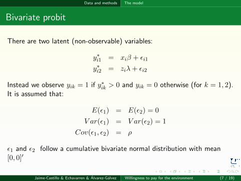
Data and methods The model

Bivariate probit

There are two latent (non-observable) variables:

y∗i1 = xiβ + εi1

y∗i2 = ziλ+ εi2

Instead we observe yik = 1 if y∗ik > 0 and yik = 0 otherwise (for k = 1, 2).It is assumed that:

E(ε1) = E(ε2) = 0

V ar(ε1) = V ar(ε2) = 1

Cov(ε1, ε2) = ρ

ε1 and ε2 follow a cumulative bivariate normal distribution with mean[0, 0]′



Two-level model

Now, let consider the two-level model for the latent variables:

y∗ij1 = xijβ + uj1 + εi1

y∗ij2 = zijλ+ uj2 + εi2

Errors are distributed as (εij1, εij2)′ ∼ N(0,Σ) and (uj1, uj2)

′ ∼ N(0,Ω):

Σ =

(σ2ε1σε1ε2 σ2ε2

), Ω =

(τ21τ12 τ22

)and they are assumed to be independent across levels:

Covij (εijk, ujk) = 0, ∀ i, j, k



Correlations

Intra-class correlation (ICC):

ρ(yijk, yi′jk

)=

τ2kσ2εk + τ2k

Correlation between two variables for the same individual:

ρ (yij1, yij2) =(σε1ε2 + τ12)√(

σ2ε1 + τ21) (σ2ε2 + τ22

)Correlation between two variables for two different individuals within thesame cluster:

ρ(yij1, yi′j2

)=

τ12√(σ2ε1 + τ21

) (σ2ε2 + τ22

)Jaime-Castillo & Echavarren & Alvarez-Galvez Willingness to pay for the environment (9 / 19)

Data and methods Estimation

Estimation using GLLAMM

For continuous outcomes xtmixed can be used to estimate suchmodels. However, for categorical outcomes the only option was to usegllamm. In Stata 13 gsem allows to model categorical outcomes

We stack both the dependent and the explanatory variables anddefine a three-level model in which k denotes the response variable, iis the individual and j is the country

First we define equations for random effects at individual and countrylevels for intercepts econs and rcons:

eq fac: econs rcons

constraint def 1 [id1_1]rcons=1

eq econs: econs

eq rcons: rcons



Estimation using GLLAMM

We constrain the loading of the second factor, because the first one isalready fixed by gllamm

The following model is estimated with gllamm:

gllamm resp2 elninc eeducyrs efemale eage eunemp eunion eenvaw ///

econs rlninc reducyrs rfemale rage runemp runion rcons, ///

i(id v4) eqs(fac econs rcons) nrf(1 2) nocons ///

family(binomial) link(probit) constr(1) adapt ip(g) nip(21)

Explanataroy variables are denoted by e for environmental taxes andby r for redistributive taxes. The model does not include intercept,since we have defined intercepts for each equationIndividuals are identified by id and countries by v4

We use adaptive Gaussian quadrature with 21 integration points. Ittakes one week!!



Estimated variances

gllamm estimates the following variance structure:

Variances and covariances of random effects

------------------------------------------------------------------------------

***level 2 (id)

var(1): .15537817 (.02648068)

loadings for random effect 1

econs: 1 (fixed)

rcons: 1 (0)

***level 3 (v4)

var(1): .05597373 (.01981084)

cov(2,1): -.00734886 (.02031006) cor(2,1): -.11561144

var(2): .07218617 (.02400351)

------------------------------------------------------------------------------



Coefficients and variances

Since the variance of econs is not constrained to 1 (as it should be in aprobit model), we need to rescale the coefficients reported by gllamm:

nlcom (elninc: [resp2]elninc/sqrt(1+[id1_1]econs^2))

Variances, covariances and correlations are obtained using nlcom:

nlcom (cov: 1-([id1_1]rcons/sqrt(([id1_1]rcons^2+[id1_1]econs^2)*(1+[id1_1]econs^2))))

nlcom (rho: (1-([id1_1]rcons/sqrt(([id1_1]rcons^2+[id1_1]econs^2)*(1+[id1_1]econs^2)))) ///

/sqrt([id1_1]econs^2*[id1_1]rcons^2))

nlcom (var21: [v42_1]econs^2)

nlcom (var22: [v42_2]rcons^2+[v42_2_1]_cons^2)

nlcom (cov2: [v42_2_1]_cons*[v42_1]econs)

nlcom (rho2: ([v42_2_1]_cons*[v42_1]econs)/([v42_1]econs*sqrt([v42_2]rcons^2 ///

+[v42_2_1]_cons^2)))

nlcom (icc_e: [v42_1]econs^2/([id1_1]econs^2+[v42_1]econs^2))

nlcom (icc_r: ([v42_2]rcons^2+[v42_2_1]_cons^2)/([id1_1]rcons^2 ///

+([v42_2]rcons^2+[v42_2_1]_cons^2)))

nlcom (corr_i: ((1-[id1_1]rcons/sqrt(([id1_1]rcons^2+[id1_1]econs^2)*(1+[id1_1]econs^2))) ///

+([v42_2_1]_cons*[v42_1]econs))/sqrt(([id1_1]econs^2+[v42_1]econs^2)*([id1_1]rcons^2 ///

+([v42_2]rcons^2+[v42_2_1]_cons^2))))

nlcom (corr_j: ([v42_2_1]_cons*[v42_1]econs)/sqrt(([id1_1]econs^2+[v42_1]econs^2)*([id1_1]rcons^2 ///

+([v42_2]rcons^2+[v42_2_1]_cons^2))))


Findings

Preferences for taxes. Linear model

(u = 0, ρ 6= 0) (u 6= 0, ρ = 0) (u 6= 0, ρ 6= 0)e r e r e r

Income 0.134*** -0.412*** 0.109*** -0.343*** 0.108*** -0.345***(0.021) (0.021) (0.023) (0.023) (0.023) (0.023)

Years of education 0.032*** -0.015*** 0.033*** -0.017*** 0.033*** -0.017***(0.003) (0.003) (0.003) (0.003) (0.003) (0.003)

Female -0.028 0.161*** -0.024 0.170*** -0.023 0.17***(0.024) (0.024) (0.023) (0.024) (0.023) (0.024)

Age 0.005*** -0.001 0.004*** 0.000 0.004*** 0.000(0.001) (0.001) (0.001) (0.001) (0.001) (0.001)

Unemployed -0.041 -0.024 -0.039 0.001 -0.039 -0.001(0.031) (0.032) (0.031) (0.031) (0.031) (0.032)

Union member -0.051** 0.214*** -0.015 0.211*** -0.013 0.208***(0.025) (0.025) (0.027) (0.027) (0.027) (0.027)

Environmental awareness 0.324*** 0.322*** 0.316***(0.013) (0.013) (0.013)

Constant -0.525** 8.037*** -0.267 7.279*** -0.229 7.421***(0.215) (0.218) (0.247) (0.251) (0.247) (0.243)

Corr(Y (e), Y (r)

)0.073*** 0.084***

(0.011) (0.011)

Corr(Y (e), Y (r)|u

)0.063***

(0.024)

Corr(u(e), u(r)

)-0.268

(0.331)

ICC(e) 0.061***(0.015)

ICC(r) 0.058***(0.022)


Findings

Preferences for taxes. Bivariate probit

(u = 0, ρ 6= 0) (u 6= 0, ρ = 0) (u 6= 0, ρ 6= 0)e r e r e r

Income 0.146*** -0.438*** 0.110*** -0.367*** 0.111*** -0.367***(0.027) (0.025) (0.030) (0.028) (0.03) (0.028)

Years of education 0.040*** -0.013*** 0.041*** -0.016*** 0.041*** -0.016***(0.004) (0.004) (0.004) (0.004) (0.004) (0.004)

Female -0.092*** 0.172*** -0.088*** 0.189*** -0.084*** 0.189***(0.031) (0.028) (0.031) (0.029) (0.031) (0.029)

Age 0.005*** 0.001 0.004*** 0.001 0.004*** 0.001(0.001) (0.001) (0.001) (0.001) (0.001) (0.001)

Unemployed -0.077* -0.048 -0.080* -0.021 -0.079* -0.021(0.041) (0.038) (0.042) (0.039) (0.042) (0.039)

Union member -0.077** 0.189*** -0.019 0.204*** -0.019 0.201***(0.032) (0.030) (0.036) (0.033) (0.036) (0.033)

Environmental awareness 0.327*** 0.332*** 0.325***(0.018) (0.018) (0.018)

Constant -3.970*** 4.996*** -3.658*** 4.217*** -3.619*** 4.242***(0.284) (0.265) (0.326) (0.308) (0.331) (0.302)

Corr(Y (e), Y (r)

)0.332*** 0.341***

(0.022) (0.021)

Corr(Y (e), Y (r)|u

)0.267***

(0.054)

Corr(u(e), u(r)

)-0.116

(0.3206)

ICC(e) 0.265***(0.075)

ICC(r) 0.067***(0.021)


Findings

Income and preferences for taxes


Findings

Education and preferences for taxes


Conclusions

Conclusions

Main findings

Preferences for environmental and redistributive taxes are linked, butthere is variability between countries

Income and education increase support for environmental taxes whilethey reduce support for redistributive taxes

Methodological issues

Multilevel models for correlated categorical outcomes are relevant inmany situations in social research, but they are difficult to estimate

gllamm performs well for our research problem, although it is slow.


Thank you. Comments are welcomed!!


distributive conflicts and willingness to pay for the … 1 theoretical approach 2 data and methods...

Documents