distributional impacts of dynamic responses to climate ...contributions of this work 1.develop a...

Motivation Estimation Approach Data and Summary Statistics Intended contributions Appendix

Distributional Impacts of Dynamic Responses toClimate Policy in the Electricity Industry

Paige Weber

Yale University, School of Forestry & Environmental Studies

Camp Resources - August 2017

Paige Weber Dynamic Responses to GHG Regulation 1 / 18


Research Question & Motivation

How does a cap-and-trade program for greenhouses gases impactthe distribution of local air pollution?



Expected responses of the electricity industry tocap-and-trade

1. Redistribution of market share to low-emission intensityunits

→ change in unit capacity factors

2. Decrease in carbon emissions intensities

→ investments to improve to unit efficiency (reduce heatrate) in natural gas dominated markets; fuel switching inmarkets with coal



Model and identification

Firms, as single-agents, makes two decisions in each period:

I Decides whether to operate → determines production quantity

I Decides whether invest to improve its efficiency → determines next periodheat rate

I Per period profits constructed a function of state variables includinglagged operating state and investment decision

Identification of unknown structural parameters:

I Start-up costs are identified by the willingness of the generator to operatein two states that differ only in last period operating decision

I Investment costs are identified by difference in heat rates across differentmarginal costs (carbon prices)

I Firm Decision 1 Firm Decision 2 Per Period Profits State Transition and Timing



Estimation approach

I Two-step estimation approach

Use Bajari, Benkard, and Levin (2007) approach to estimatepolicy functions for production and investment decisions;develop approximation of electricity price paths incounterfactuals.



Data

I Prices: Hourly wholesale electricity prices from CAISO;carbon allowance prices: ICE; fuel input prices: federalreporting requirements and Bloomberg coal/natural gas spotprices

I Production quantities: Unit-specific hourly electricity outputfrom CEMS

I Emission quantities: Hourly emissions of NOx ,SO2,CO2

from CEMS

I Unit characteristics: various EIA reporting requirements



Average profits per hour, 2012-2016

-500

050

010

0015

0020

00$

Profi

ts

0 2 4 6 8 10 12 14 16 18 20 22Hour of the Day



Carbon prices over time



Input fuel prices over time



Capacity factors for sample month (Sept.), 2012 - 2016

2012 2013 2014 2015 2016



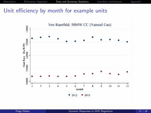
Unit efficiency by month for example units



Heat rates for sample month (Sept.), 2012 - 2016

September Heat Rates (Reported)

2012 2013 2014 2015 2016



Contributions of this work

1. Develop a dynamic model of electric generating behavior that includesboth production and investment.

2. Simulate counterfactual outcomes of redistribution and investment inefficiency under different GHG policy scenarios (e.g. a more stringentpolicy with higher prices, a command and control approach).

3. Map market outcomes across carbon policy scenarios to local air qualityoutcomes and damages to human health (leveraging epidemiological workand/or AP2 (APEEP) model).



Per Period Profits

πt(q(ait),Pt ,Cit , Γit , Lit) =

qit(Pt − Ct(hrit ,mcf , eg , τt))− Γ(zit , vit ; γi ), ait = 1, Lit = 1

qit(Pt − Ct(hrit ,mcf , eg , τt))− Γ(zit , vit ; γi )− starti , ait = 1, Lit = 0

0, ait = 0

(1)

I starti : start-up costs incurred when turning on after lagged operating stateLit = ait−1 = 0

I Pt : exogenous hourly price (to be discussed)

I Ct(·): marginal cost function:

Ct = hrit ∗mcf + hrit ∗ ef τt (2)

I hrit : heat rate, mcf : marginal costs of fuel, eg : emissions rate of fuel, τt : GHGemissions permit price

I Γt(·): cost of investment (previous slide)



Firm Decision 1: Operation (production) choice

Firm i = 1, ...,N makes operating decision ait ∈ {0, 1} in eachhour t which determines qit

qit = qmax ,i if Pt ≥ Cit and ait = 1

qit = qmin,i if Pt < Cit and ait = 1(3)

I qit : MWh produced by firm i if hour t

I qmax(min),i : unit-specific production constraint

I Pt : wholesale electricity price in hour t

I Cit : marginal cost of electricity

Back to Back to Model Overview



Firm Decision 2: Investment choice

When ait = 1, firm makes an investment decisions zit ∈ R+, whichimproves the efficiency (reduces the heat rate) hrit+1 with cost Γ(·)

hrit+1 = hrit(1 + δ)− zit

Γ(zit , hrit , γi , vit) = 1(zit > 0)(γg(i)1 + γg(i)2zithrit

+ vit)(4)

I δ: depreciation rate

I γg(i)1, γg(i)2: fixed and variable costs of investment for technology group g(i)

I vit : stochastic shock to investment costs




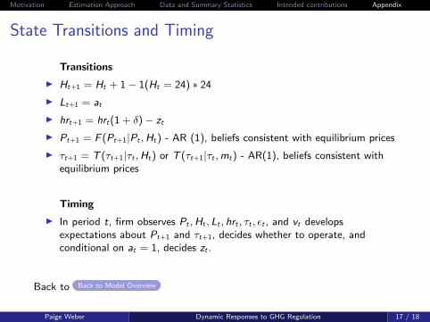
State Transitions and Timing

Transitions

I Ht+1 = Ht + 1− 1(Ht = 24) ∗ 24

I Lt+1 = at

I hrt+1 = hrt(1 + δ)− zt

I Pt+1 = F (Pt+1|Pt ,Ht) - AR (1), beliefs consistent with equilibrium prices

I τt+1 = T (τt+1|τt ,Ht) or T (τt+1|τt ,mt) - AR(1), beliefs consistent withequilibrium prices

Timing

I In period t, firm observes Pt ,Ht , Lt , hrt , τt , εt , and vt developsexpectations about Pt+1 and τt+1, decides whether to operate, andconditional on at = 1, decides zt .




Intertemporal Problem

I Firms choose at and zt to maximize the sum of discounted profits:

V (st) = maxat ,zt

Σ∞j=0βjΠ(at+j , zt+j , st+j |at+j , zt+j , st)

st = {xt ; et} = {Pt ,Ht , Lt , hrt , τt ; ε(at), vt}(5)

I The Bellman equation for this dynamic programming problem is:

V (st) = maxat ,zt{Π(st , at , zt) + βE [V (st+1)|at , zt , st ] (6)

E [V (st+1)|at , zt , st ] =

∫V (Pt+1,Ht+1, Lt+1, hrt+1, τt+1; εt+1(at+1), vt+1|Pt ,Ht , Lt , hrt , τt)[...]

dP(εt+1(at+1), vt+1,Pt+1, τt+1)

(7)



distributional impacts of dynamic responses to climate ...contributions of this work 1.develop a...

Documents