distribution of missing sums in sumsets
TRANSCRIPT

DISTRIBUTION OF MISSING SUMS IN SUMSETS
OLEG LAZAREV, STEVEN J. MILLER, AND KEVIN O’BRYANT
ABSTRACT. For any finite set of integersX , define its sumsetX + X to be{x + y : x, y ∈ X}.In a recent paper, Martin and O’Bryant investigated the distribution of |A + A| given the uniformdistribution on subsetsA ⊆ {0, 1, . . . , n − 1}. They also conjectured the existence of a limitingdistribution for|A+A| and showed that the expectation of|A+A| is 2n−11+O((3/4)n/2). Zhaoproved that the limitsm(k) := limn→∞ P (2n− 1− |A+A| = k) exist, and that
∑k≥0
m(k) = 1.We continue this program and give exponentially decaying upper and lower bounds onm(k),
and sharp bounds onm(k) for smallk. Surprisingly, the distribution is at least bimodal; sumsetshave an unexpected bias against missing exactly 7 sums. The proof of the latter is by reduction toquestions on the distribution of related random variables,with large scale numerical computationsa key ingredient in the analysis. We also derive an explicit formula for the variance of|A + A| interms of Fibonacci numbers, findingVar(|A + A|) ≈ 35.9658. New difficulties arise in the formof weak dependence between events of the form{x ∈ A + A}, {y ∈ A + A}. We surmount theseobstructions by translating the problem to graph theory. This approach also yields good bounds onthe probability forA+ A missing a consecutive block of lengthk.
CONTENTS
1. Introduction 21.1. Terminology and Theorems 31.2. Variance and Decay Rates of Missing Sums 41.3. Other types of random sets and the divot 62. Graph-Theoretic Framework 83. Variance of Missing Sums 94. Exponential Bounds 175. ApproximatingP(k + a1, k + a2, . . . , andk + am 6∈ A+ A) 206. Consecutive Missing Sums 237. Bounds onm(k), w(k), y(k), andz(k) for k < 32 277.1. Making the computation feasible, reliable, and verifiable 317.2. Obtainingy(k), m(k), andw(k) from z(k) 328. Conjectures and Future Research 34Appendix A. Data tables for distributions 36References 40
Date: October 20, 2012.2010Mathematics Subject Classification.11P99 (primary), 11K99 (secondary).Key words and phrases.sumsets, uniformly random sumsets, Fekete’s Lemma.We thank the participants of the SMALL 2011 REU at Williams College for many enlightening conversations,
and the referee for many helpful comments on an earlier draft. The first named author was supported by NSF grantsDMS0850577 and Williams College; the second named author was partially supported by NSF grant DMS0970067.This research was supported, in part, under National Science Foundation Grants CNS-0958379 and CNS-0855217 andthe City University of New York High Performance Computing Center.
1

1. INTRODUCTION
The central object of additive number theory [N,TV] is the sumsetX+X of a setX of integers:
X +X := {x1 + x2 : x1, x2 ∈ X}. (1.1)
Typically, the theory is concerned with extremal behavior,such as the structure of finiteX when|X + X|/|X| is nearly minimal (Freiman’s Theorem), or the possible densities ofX when|X +
X|/(|X|+1
2
)is maximized (Sidon Sets). See [N,R] for surveys and [F,J] for examples.
Here we focus ontypicalbehavior: for a randomly chosen setX of integers, what is the expectedvalue and variance of|X +X|? The answer of course depends on howX is chosen, and we focusour attention on sets taken uniformly from the2n subsets of[0, n − 1]; we denote intervals ofintegers as[a, b] := {x ∈ Z : a ≤ x ≤ b} and such a random set asA. In §1.3 and §7.2 we discusssome variations on the manner of choosing a random set of natural numbers.
Other authors have considered aspects of typical behavior of sumsets. When Erdos and Rényi[ER] first applied the probabilistic method to number theory, they observed that with probability1, a uniformly random subsetC of N will haveC +C = N \ F for somefinitesetF , but made noeffort to exploreF further. The present work concerns itself with properties of the set
Fn := [0, 2n− 2] \ (A+ A),
with A as above. We prove the existence of
limn→∞
E [|Fn|r]for everyr ≥ 1, give upper and lower bounds on
P (|Fn| = k)
for smallk, largen, and also ask → ∞, and also bound
P ({a1, a2, . . . , ak} ⊆ Fn) .
Our work is usually quantitatively effective, and we reportnumerical estimates throughout.The key obstacle to finding the limiting distribution of|Fn| is the dependence between different
elements occurring or not occurring inA + A. For example,3 6∈ A + A and7 6∈ A + A are de-pendent events since both are affected by whether2 ∈ A. We develop a graph theoretic frameworkwhich makes it much easier to analyze the dependence betweensuch events and to develop boundsthat incorporate the dependence. It is possible to avoid this framework, but doing so makes bothnotation and the underlying issues less clear.
Graph theory has been used in additive number theory before.For example, Plünnecke (see thedescription in [R]) uses graph theory to estimate the size ofk-fold sumsets in terms of|A| and|A+ A|, Alon and Erdös [AE] use hypergraphs to study Sidon sets, andGilbert [G] on the Erdos-Turan conjecture. Our use of graph theory seems to be different from these as we investigate thesize ofA+ A for typicalA, without reference to the size ofA itself.
The next subsection of this introduction sets up our notation and states our main results. The lasttwo subsections provide more motivation and indicate the nature of our proofs and computations.In §2, we develop a graph theoretic framework for handling the dependencies between events like{a1 ∈ F} and{a2 ∈ F}. In §3, we find an explicit formula for the limit of the variance of |F | andprove Theorem 1.5, stated below. In §4, we prove the exponential bounds for Theorem 1.2. In §5,we find the probability of missing certain configurations andprove Theorem 1.6, while in §6 wediscuss consecutive missing elements and prove Theorem 1.7and Theorem 1.8. We return to the
2

problem of explicit bounds onP (|Fn| = k) for smallk and the existence of a limiting distributionfor |Fn| in §7. Finally in §8, we discuss some problems for future research and how the graphtheoretic framework may be applied to such problems.
Remark 1.1. Many of the questions in this paper grew out of studying the difference in size betweenthe sumsetA+A and the difference setA−A. As addition is commutative and subtraction is not,it is natural to expect the difference set of a typicalA drawn uniformly from{0, 1, . . . , n} to belarger than the sumset. Though numerical exploration and heuristics suggested that almost all setsshould give rise to more differences, Martin and O’Bryant[MO] proved that a small but positivepercentage are sum-dominant. The percentage is quite small, around4.5 ·10−4 [Z] . Understandingthe structure ofA + A, in particular when and what sums are missing, has motivatedmuch of thetheoretical and numerical work in the field. For other directions, see[HM] for results on non-uniform models or[ILMZ] for multiple comparisons and summands.
1.1. Terminology and Theorems. The main characteristic ofA+A is that it is almost full. Martinand O’Bryant [MO] proved that
E [|A+ A|] = 2n− 1− 10 +O((3/4)n/2
). (1.2)
Since typical sumsets are almost full, it is more natural to investigate the number of missing sums,which is why we write the above as2n − 1 minus 10. As noted in [MO], sumsets are almost fullbecause middle elements have many representations as a sum of two elements of[0, n − 1]; eachi ∈ [0, 2n− 2] has roughlyn/4− |n− i|/4 representations.
We set
M[0,n−1] := |[0, 2n− 2] \ (A+ A)| = 2n− 1− |A+ A|,mn(k) := P
(M[0,n−1] = k
),
m(k) := limn→∞
mn(k). (1.3)
A special case of Zhao’s theorem [Z] is thatm(k) is well-defined, strictly positive, and that∑∞k=0m(k) = 1, so that we can think ofm(k) as defining a distribution onN. Thus, we can
speak of “the probability that a large finite setX has a sumset that misses exactly 17 elements”and mean something sensible. Zhao’s work is numerically impractical and did not give reasonableupper bounds onm(k); we do that in §7, where we also reprove Zhao’s results in thiseasier setting.See Figure 1 for the experimental estimates and rigorous bounds onm(k) for 0 ≤ k < 32.
The result (1.2) above implies that
limn→∞
E[M[0,n−1]
]= 10.
Equivalently, in light of Zhao’s work,∑∞
k=0 km(k) = 10. To this, we add the following results.Let φ := (1 +
√5)/2, the golden ratio.
Theorem 1.2.Letn > 5k. Then
2−k/2 ≪ mn(k) ≪ (φ/2)k, (1.4)
where the implied constants are independent ofk andn.
Note that2−1/2 ≈ 0.707 andφ/2 ≈ 0.809, so that bounds provided by Theorem 1.2 are reason-ably close. We suspect, based on numerical data, that the following conjecture represents the truthof the matter, and perhaps evenλ =
√φ− 1.
3

0 5 10 15 20 25 30k
0.01
0.02
0.03
0.04
0.05
0.06
0.07
mHkL
FIGURE 1. Experimental values ofm(k), with vertical bars depicting the valuesallowed by our rigorous bounds. In most cases, the allowed interval is smaller thanthe dot indicating the experimental value. The data comes from generating228 setsuniformly forced to contain 0 from[0, 256); see §7.2 for details of the calculation.
Conjecture 1.3. There existsλ such that for anyǫ > 0,
(λ− ǫ)k ≪ǫ m(k) ≪ǫ (λ+ ǫ)k. (1.5)
From numerical data,λ ≈ 0.78.
The exponential bounds of Theorem 1.2 already imply that therth moment remains bounded foranyr ≥ 1.
Corollary 1.4. The limit of therth moment ofM[0,n−1],
limn→∞
E[M r
[0,n−1]
], (1.6)
exists and is finite.
Theorem 1.5.The limitlimn→∞
Var(M[0,n−1]
)(1.7)
exists and is about35.9658, as these are the first digits of its decimal expansion. This limit can bewritten as the following convergent series with exponential decay:
limn→∞
Var(M[0,n−1]
)= 4 lim
n→∞
∑
i<j<n
P(i andj 6∈ A+ A)− 40. (1.8)
Note that “i andj 6∈ A + A” is meant to be parsed as “(i 6∈ A+ A) AND (j 6∈ A+ A)”.
1.2. Variance and Decay Rates of Missing Sums.The bounds in Theorem 1.2 are due to formu-las for probabilities of events such as
P(a1, a2, . . . , andam 6∈ A+ A), (1.9)
by which we mean the probability that all ofa1, a2, . . . , am are in the complement ofA+ A. Thisrepresents the probability that a particular configurationis not inA + A. As long asn > am,
4

there is no dependence onn since this probability just depends on[0, am] ∩ A. We thereforecan assume thatA ⊆ [0, am]. Formulas for such probabilities are also important for finding themoments ofM[0,n−1]. For example, to find the expectation of|A+A|, [MO] find an exact formulafor P(k 6∈ A+ A), which is approximately
P(k 6∈ A+ A) = Θ((3/4)k/2), (1.10)
where we sayg(n) = Θ(f(n)) if there exist constantsC1, C2 such that for alln
C1f(n) ≤ g(n) ≤ C2f(n). (1.11)
Similarly, to find the variance, we can studyP(i andj 6∈ A+A) as seen from the series expansionin (1.8). In Proposition 3.5, we find an exact formula for thisprobability and in Corollary 3.6, weshow that for fixedm we have the following approximation:
P(k andk +m 6∈ A+ A) = Θ((φ/2)k). (1.12)
The implied constants in (1.12) depend significantly onm and in Corollary 3.6, we also find theseconstants.
Note that both (1.10) and (1.12) are exponential ink. In fact, we prove that in general suchprobabilities are approximately exponential ink.
Theorem 1.6.For any fixeda1, . . . , am, there existsλa1,...,am such that
P(k + a1, k + a2, . . . , andk + am 6∈ A+ A) = Θ(λka1,...,am), (1.13)
where the implied constants depend ona1, . . . , am but notk.
The fact thatP(k+a1, k+a2, . . . , andk+am 6∈ A+A) is approximately exponential supportsConjecture 1.3 that the distribution of missing sums is approximately exponential.
For the particular configurationa1 = 1, a2 = 2, . . . , am = m, the case of consecutive missingelements, we can approximateλa1,...,am well as seen in the following theorem.
Theorem 1.7.For anyk,m(1
2
)(k+m)/2
≪ P(k + 1, k + 2, . . . , andk +m 6∈ A+ A) ≪(1
2
)(k+m)/2
(1 + ǫm)k, (1.14)
with ǫm → 0 asm → ∞. To be more precise, the exact form of upper bound is(1/2)(k+m)/22k/m.This implies that
λ0,1,2,...,m →(1
2
)1/2
(1.15)
asm → ∞.
As we will see in the proof of Theorem 1.2, the lower bound(1/2)(k+m)/2 is essentially theprobability of missing the firstk +m elements inA + A. By Theorem 1.7, we have that for largem, P(k + 1, k + 2, . . . , andk +m 6∈ A+A) is also approximately(1/2)(k+m)/2. This means thatfor largem, essentially the only way to missm consecutive elements inA+ A starting atk + 1 isthrough the trivial way - namely missing all of the firstk +m elements ofA + A.
Theorem 1.7 is in fact a special case of the following inequality.
Theorem 1.8.For λa1,...,am with 0 ≤ a1 < · · · < am,
λa1,...,am ≤ P(A,B ⊆ [0, ⌊am/2⌋] | a1, . . . , am 6∈ A+B)1
am+2 . (1.16)
whereA,B are two independently chosen sets.5
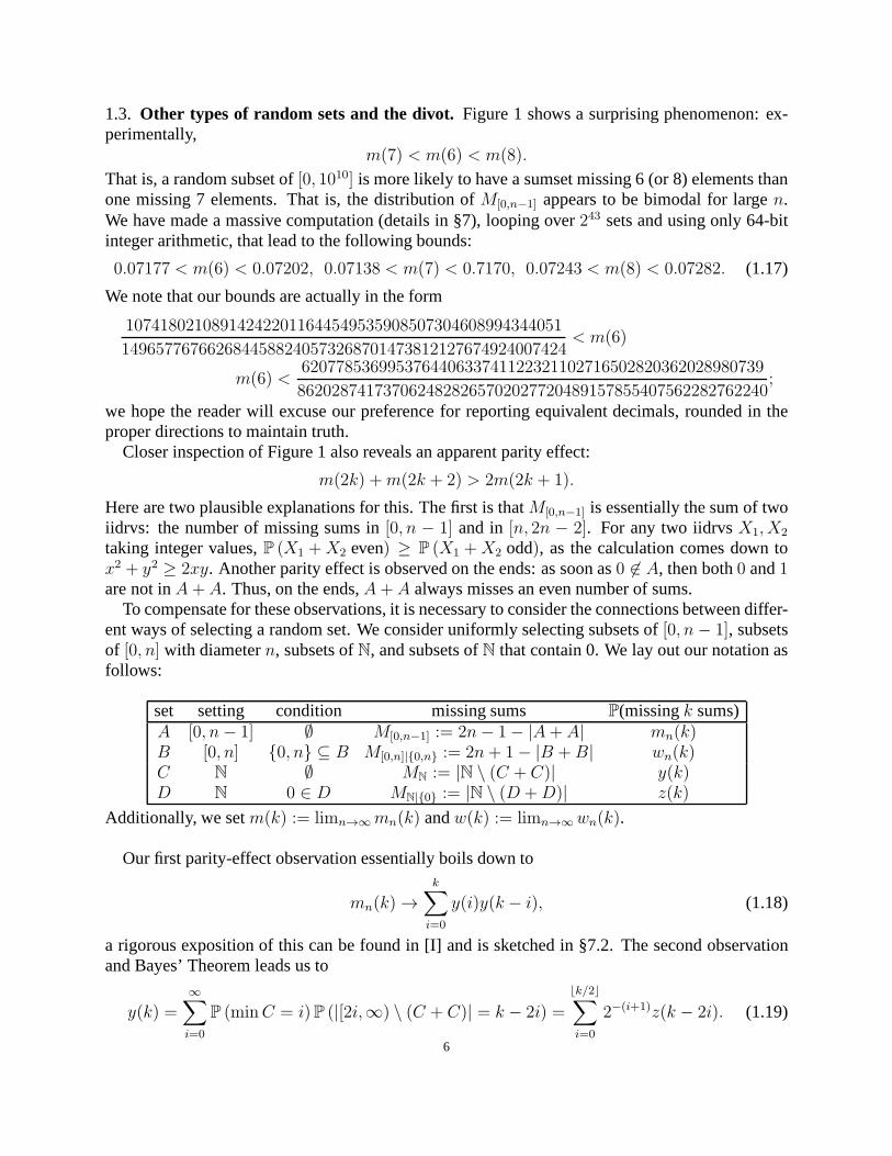
1.3. Other types of random sets and the divot.Figure 1 shows a surprising phenomenon: ex-perimentally,
m(7) < m(6) < m(8).
That is, a random subset of[0, 1010] is more likely to have a sumset missing 6 (or 8) elements thanone missing 7 elements. That is, the distribution ofM[0,n−1] appears to be bimodal for largen.We have made a massive computation (details in §7), looping over 243 sets and using only 64-bitinteger arithmetic, that lead to the following bounds:
0.07177 < m(6) < 0.07202, 0.07138 < m(7) < 0.7170, 0.07243 < m(8) < 0.07282. (1.17)
We note that our bounds are actually in the form
107418021089142422011644549535908507304608994344051
1496577676626844588240573268701473812127674924007424< m(6)
m(6) <620778536995376440633741122321102716502820362028980739
8620287417370624828265702027720489157855407562282762240;
we hope the reader will excuse our preference for reporting equivalent decimals, rounded in theproper directions to maintain truth.
Closer inspection of Figure 1 also reveals an apparent parity effect:
m(2k) +m(2k + 2) > 2m(2k + 1).
Here are two plausible explanations for this. The first is that M[0,n−1] is essentially the sum of twoiidrvs: the number of missing sums in[0, n − 1] and in [n, 2n − 2]. For any two iidrvsX1, X2
taking integer values,P (X1 +X2 even) ≥ P (X1 +X2 odd), as the calculation comes down tox2 + y2 ≥ 2xy. Another parity effect is observed on the ends: as soon as0 6∈ A, then both0 and1are not inA+ A. Thus, on the ends,A+ A always misses an even number of sums.
To compensate for these observations, it is necessary to consider the connections between differ-ent ways of selecting a random set. We consider uniformly selecting subsets of[0, n− 1], subsetsof [0, n] with diametern, subsets ofN, and subsets ofN that contain 0. We lay out our notation asfollows:
set setting condition missing sums P(missingk sums)A [0, n− 1] ∅ M[0,n−1] := 2n− 1− |A+ A| mn(k)B [0, n] {0, n} ⊆ B M[0,n]|{0,n} := 2n+ 1− |B +B| wn(k)C N ∅ MN := |N \ (C + C)| y(k)D N 0 ∈ D MN|{0} := |N \ (D +D)| z(k)
Additionally, we setm(k) := limn→∞mn(k) andw(k) := limn→∞wn(k).
Our first parity-effect observation essentially boils downto
mn(k) →k∑
i=0
y(i)y(k − i), (1.18)
a rigorous exposition of this can be found in [I] and is sketched in §7.2. The second observationand Bayes’ Theorem leads us to
y(k) =∞∑
i=0
P (minC = i)P (|[2i,∞) \ (C + C)| = k − 2i) =
⌊k/2⌋∑
i=0
2−(i+1)z(k − 2i). (1.19)
6

0 5 10 15 20 25 30k
0.01
0.02
0.03
0.04
0.05
0.06
0.07
mHkL
0 5 10 15 20 25 30k
0.02
0.04
0.06
0.08
0.10
wHkL
0 5 10 15 20 25 30k
0.02
0.04
0.06
0.08
0.10
0.12
0.14yHkL
0 5 10 15 20 25 30k
0.05
0.10
0.15
0.20
0.25zHkL
FIGURE 2. Experimental values ofm(k), w(k), y(k), z(k), with vertical bars de-picting the values allowed by our rigorous bounds. See §7 fordetails.
Similarly to (1.18), one can prove that
wn(k) →k∑
i=0
z(i)z(k − i). (1.20)
Thus, all four distributions can be understood in terms ofz(k). Experiments and our bounds (seeFigure 2 for small values ofk) indicate thatMN|{0} has an approximately geometric distribution,and exhibits no obvious parity effect. Computationally, wefocus on boundingz and then allowthis to determine bounds onm, w andy.
We boundz by conditioning onI := D∩[0, 44), and loop over all243 possible values ofI (a pri-ori, 0 ∈ I). For eachI ⊆ [0, 44), we explicitly know(D+D)∩ [0, 44), we have much informationconcerning(D+D)∩[44, 88), and theoretically(D+D)∩[88,∞) is [88,∞)with high probability.This allows us to give reasonable upper and lower bounds onP
(MN|{0} = k | D ∩ [0, 44) = I
)for
eachI.If we suppose thatMN|{0} is exactly geometric with parameterλ (i.e., setz(k) = (1 − λ)λk)
and definey(k) andm(k) using (1.18) and (1.19), we find that the distribution ofMN|{0} wouldbe bimodal with a divot atk = 7 only for the narrow parameter range0.756 < λ < 0.771.The best-squares fit forλ is 0.765. If we suppose thatMN|{0} has a Poisson distribution, i.e.,z(k) = λke−λ/k!, we find that there are noλ whatsoever that give a bimodal distribution withdivot atk = 7.
This implies that the divot’s existence relies not only on the above observations but also on thespecific values ofzk for small values. We note thatz4 in particular is larger than the geometric
7

model predicts; more than half of the least-squares error isfrom z4. The rigorous bounds we givealso show this bias towards 4, though we currently have no understanding as to why this is thesituation.
Theorem 1.9. The limits definingm(k) andw(k) are well-defined, positive, and∑∞
k=0m(k) =∑∞k=0w(k) = 1. Rigorous bounds onm(k), w(k), y(k) and z(k) for 0 ≤ k < 32 are given in
Appendix A. In particular,m(7) < m(6) < m(8).
2. GRAPH-THEORETIC FRAMEWORK
We first develop a graph-theoretic framework to study dependent random variables and calculateprobabilities likeP(a1, . . . , andam 6∈ A+ A). Note that for oddi
{i 6∈ A+ A} = {(0 6∈ A or i 6∈ A) and · · · and ((i− 1)/2 6∈ A or (i+ 1)/2 6∈ A)} , (2.1)
and for eveni
{i 6∈ A + A} = {(0 6∈ A or i 6∈ A) and · · · and (i/2− 1 6∈ A or i/2 + 1 6∈ A) andi/2 6∈ A}.(2.2)
Therefore for distincti the events{i 6∈ A + A} are dependent as both depend on conditions onAlike {0 6∈ A}.
For example, the conditions onA necessary for{3 and7 6∈ A+ A} are
i = 3 : 0 or 3 6∈ A j = 7 : 0 or 7 6∈ Aand1 or 2 6∈ A and1 or 6 6∈ A
and2 or 5 6∈ Aand3 or 4 6∈ A.
(2.3)
Since the two lists have integers in common, there is dependence between the events{3 6∈ A+A}and{7 6∈ A+ A}.
We construct a graph to represent the dependencies between the random variables. We call thisgraph thecondition graphfor the probability. We construct the condition graph forP(a1, . . . , andam 6 ∈ A+ A), wherea1 < · · · < am, in the following way:
(1) For every integer in[0, am], add a vertex labeled with that integer.(2) Add an edge between two vertices labeled withi andj if i+ j = ak for some1 ≤ k ≤ m.
See Figure 3 for the condition graph forP(3 and7 6∈ A+ A).
01
2
34
5
6
7
FIGURE 3. Condition Graph forP(3 and7 6∈ A + A).
By construction, we have a one-to-one correspondence between edges and conditions and ver-tices and integers in[0, am]. For example, the edge between vertices labeled with1 and6 representsthe condition that1 or 6 6∈ A, which is one of the conditions necessary for7 6∈ A+A in (2.3). For
8

each condition, we need to pick at least one element to exclude fromA. Therefore in the conditiongraph, for each edge we need to pick at least one of its vertices. That is, we need to pick a vertexcover (recall a vertex cover of a graph is a set of vertices such that each edge is incident to at leastone vertex in the set). Using this method, we get the following lemma.
Lemma 2.1. P(a1, . . . , andam 6∈ A + A) equals the probability that we chose a vertex cover forthe condition graph.
Note that when we pick vertices in the condition graph for ourvertex cover, we are picking toexclude those vertices fromA. For example, note that the vertices7, 0, 4 and6, 2 form a vertexcover for the condition graph ofP(3 and7 6∈ A + A) in Figure 3. Then if7, 0, 4, 6, 2 6∈ A, then3 and7 6∈ A+ A since all conditions in (2.3) are met.
Finally, note that when we calculate the probability of chosing a vertex cover for the conditiongraph, we no longer need to consider a labeled graph. This is because vertices represent elements ofA, and since each element ofA is equally likely to be chosen (asA is chosen uniformly randomly),we do not need to differentiate between different elements.
3. VARIANCE OF M ISSING SUMS
We now use the graph-theoretic framework from the previous section to prove Theorem 1.5 andfind the variance.
We first note that the result of [MO] in (1.2) is really that
E[M[0,n−1](A)
]=
∑
0≤i≤2n−2
P(i 6∈ A+ A) = 10 +O((3/4)n/2). (3.1)
SinceVar
(M[0,n−1](A)
)= E
[M[0,n−1](A)
2]−(E[M[0,n−1](A)
])2(3.2)
and we knowE[M[0,n−1](A)
]from (3.1), to find the variance we just need to determineE
[M[0,n−1](A)
2],
which equals the following:
E[M[0,n−1](A)
2]
=1
2n
∑
A⊆[0,n−1]
|{missing sums inA + A}|2
=1
2n
∑
A⊆[0,n−1]
∑
0≤i,j≤2n−2i,j 6∈A+A
1
=1
2n
∑
0≤i,j≤2n−2
∑
A⊆[0,n−1]i,j 6∈A+A
1
=∑
0≤i,j≤2n−2
P(A ⊆ [0, n− 1] | i andj 6∈ A+ A)
= 2∑
0≤i<j≤2n−2
P(i andj 6∈ A+ A) +∑
0≤i≤2n−2
P(i 6∈ A + A). (3.3)
Combining (3.2), (3.1), and (3.3), we get
Var(M[0,n−1](A)
)= 2
∑
0≤i<j≤2n−2
P(i andj 6∈ A+ A)− 90 +O((3/4)n/2). (3.4)
9

We first simplify the sum overi, j. Note that ifi, j < n, then
P(i andj 6∈ A + A) = P(2n− 2− i and2n− 2− j 6∈ A+ A), (3.5)
and so ∑
0≤i<j<n
P(i andj 6∈ A + A) =∑
n≤i<j≤2n−2
P(i andj 6∈ A+ A). (3.6)
Also, note that ifi < n/2 andj > 3n/2, then{i 6∈ A + A} and{j 6∈ A + A} are independent.This is because{i 6∈ A + A} depends only on[0, i] ∩ A and{j 6∈ A + A} depends only on[j − n+1, n− 1]∩A and if i < n/2 andj > 3n/2, these sets are disjoint. Therefore for suchi, j,we have
P(i andj 6∈ A+ A) = P(i 6∈ A+ A)P(j 6∈ A+ A). (3.7)
Finally note that ifn/2 ≤ i < n or n ≤ j ≤ 3n/2, then
P(i andj 6∈ A+ A) = O((3/4)n/4) (3.8)
by (1.10). Therefore∑
i<n, n≤j
P(i andj 6∈ A+ A)
=∑
i<n/2 and 3n/2<j
P(i andj 6∈ A+ A) +∑
n/2≤i<n or n≤j≤3n/2
P(i andj 6∈ A+ A)
=∑
i<n/2, 3n/2<j
P(i andj 6∈ A+ A) +O(n2(3/4)n/4)
=
∑
i<n/2
P(i 6∈ A+ A)
·
∑
3n/2<j≤2n−2
P(j 6∈ A+ A)
+O(n2(3/4)n/4)
=(5 +O((3/4)n/4)
)·(5 +O((3/4)n/4)
)+O(n2(3/4)n/4)
= 25 +O(n2(3/4)n/4), (3.9)
where we use (3.1) and (3.5) to get the second to last equality. Combining (3.6) and (3.9), we have∑
0≤i<j≤2n−2
P(i andj 6∈ A+ A)
=∑
0≤i<j<n
P(i andj 6∈ A+ A) +∑
n≤i<j≤2n−2
P(i andj 6∈ A+ A) +∑
i<n, n≤j
P(i andj 6∈ A+ A)
= 2∑
0≤i<j≤n−1
P(i andj 6∈ A+ A) + 25 +O(n2(3/4)n/4), (3.10)
and so by (3.4)
Var(M[0,n−1](A)
)= 4
∑
0≤i<j≤n−1
P(i andj 6∈ A + A)− 40 +O(n2(3/4)n/4). (3.11)
Therefore to find the variance, we just need to studyP(i andj 6∈ A+ A) for i < j < n.Since the other cases are handled similarly, we only presentthe details for the case wheni and
j are both odd.By Lemma 2.1, we just need to study the condition graph forP(i andj 6∈ A+A).10

Recall that we already found the condition graph forP(3 and7 6∈ A + A) in Figure 3. Afteruntangling this graph, we see that it really consists of two components, as seen in Figure 4.
7 0 3 4 6 1 2 5
FIGURE 4. Untangled condition graph forP(3 and7 6∈ A + A).
Also note that each component is asegment graph, a graph that consists of a sequence of verticessuch that each vertex is connected only to the vertices to itsimmediate left and right. A similarsituation holds in general, as seen by the following proposition.
Proposition 3.1. The condition graph forP(i andj 6∈ A + A) has components that are segmentgraphs.
Proof. The condition graph forP(i andj 6∈ A + A) has vertices with degree less than or equal to2; if the vertex is labeled withℓ, it can only be connected to vertices labeledi− ℓ or j − ℓ (if suchvertices exist).
Furthermore, there are no cycles in the condition graph. Suppose there is a cycle in the conditiongraph. Consider the vertex in the cycle with the maximum label ℓ and consider the vertices aroundthis vertex. Each of these vertices must have exactly two neighbors and so we have the followingsituation as seen in Figure 5.
j − ℓ ℓ i− ℓ ℓ+ j − i
FIGURE 5. Vertices around a labeled vertexℓ.
Notice thatℓ + j − i > ℓ sincej > i. Therefore,ℓ is not the maximum label, which is acontradiction and proves that we cannot have a cycle. Thus all components are trees with allvertices having degree less than or equal to2, implying that all are segment graphs. �
Since labels in different components are distinct and thereare no edges between different com-ponents, each component is independent. That is, the probability of getting a vertex cover for theentire graph is the product of the probability of getting vertex covers for each component. In thisway, we just need to find the probability of getting a vertex cover for each component. To do this,we find the number of vertex covers for an arbitrary segment graph, which we do in the followingproposition.
Proposition 3.2. The number of vertex coversg(n) for a segment graph withn vertices satisfiesg(n) = Fn+2, whereFk is thekth Fibonacci number.
Proof. There are two cases: the first vertex of the segment graph is inthe vertex cover, or it is not.If the first vertex is in the cover, then the first edge already has one of its vertices picked. Thereforewe just need a vertex cover for the subgraph withn − 1 vertices that follows the first edge, andby definition there areg(n− 1) such covers. If the first vertex is not in the cover, then the secondvertex must be the cover since the first edge must have one of its vertices chosen. Since the secondvertex is now in the cover, then the second edge automatically has one of its vertices in the cover.Therefore we just need a vertex cover for the subgraph withn− 2 vertices that follows the second
11

edge, and by definition there areg(n − 2) such vertex covers. Therefore, we have the Fibonaccirecursive relationshipg(n) = g(n− 1) + g(n− 2). As g(2) = 3 = F4 andg(3) = 5 = F5, theseinitial conditions and the recurrence implyg(n) = Fn+2, completing the proof. �
Therefore, we have
P(chose a vertex cover for a segment graph withn vertices) =Fn+2
2n. (3.12)
Returning to our example with3 and 7, we note that since the condition graph in this caseconsists of two segment graph components each of length4, we have
P(3 and7 6∈ A+ A) =F4+2
24· F4+2
24=
1
4, (3.13)
where we can multiply the probabilities by the independenceof the components.In general, as the condition graph may have many components we must find how many segment
graph components there are in the entire graph forP(i andj 6∈ A+ A).
Proposition 3.3. There are(j − i)/2 segment graph components for the graph ofP(i andj 6∈A+ A).
Proof. Note that in totalj+1 vertices are used in the graph ofP(i andj 6∈ A+A); since{i andj 6∈A+A} depends just onA∩ [0, j], the graph uses exactly the integers in[0, j]. Also note that eachcomponent must end with a vertex labeled by an integer greater thani. If a component ends with avertex labeled byℓ ≤ i, then it can be connected to two other verticesi− ℓ andj − ℓ. Rememberthat we are assumingi andj are odd (the other cases are similar). As they are odd,i − ℓ 6= ℓ andj − ℓ 6= ℓ and soi− ℓ, j − ℓ, ℓ are all distinct. Sinceℓ is connected to two other vertices, it cannotbe an end vertex. Therefore, each end vertex is labeled by some integer in[i+1, j]. Also note thateach of these integers must be end vertex since it cannot be used to add up toi. Therefore, the set[i+1, j] coincides with the set of end vertices and since each component has two end vertices withdistinct labels, there are(j − i)/2 components. �
We also need to find the length of each component. Fortunately, there are only two possiblecomponent lengths for the graph ofP(i andj 6∈ A+ A), as seen by the following lemma.
Proposition 3.4.The length of each segment graph component for the graph ofP(i andj 6∈ A+A)is always either
2
⌈i+ 1
j − i
⌉or 2
⌈i+ 1
j − i
⌉+ 2. (3.14)
Proof. First note that the difference between a given vertex and another vertex that is two edgesaway isj − i. This is because the sum of the vertices that share an edge alternates betweeni andj, so that we have segments of the form given in Figure 6. The difference betweenj − x andi− xis j − i as needed.
i− x x j − x
FIGURE 6. Difference between every other vertex.12

Now note that these differences can be used to determine the size of each component. Supposethe end vertex of a segment graph ism. Since we decrease byj− i for every two vertices and sincewe only use non-negative integers, there can only be
⌊m
j − i
⌋+ 1 =
⌈m+ 1
j − i
⌉(3.15)
decreases. Since we decrease once for every two vertices, wehave that the length is twice thenumber of decreases. Therefore the length is
2
⌈m+ 1
j − i
⌉. (3.16)
From Proposition 3.3, we also know that the end vertexm of each segment graph satisfiesi < m ≤ j. Therefore, the length of each segment graph is always
2
⌈i+ 1
j − i
⌉or 2
⌈i+ 1
j − i
⌉+ 2, (3.17)
as desired. �
For simplicity, we denote the first of the two values in (3.14)by q and the second byq + 2. Wemust find the number of components with sizeq andq+2. Suppose there arer components of sizeq andr′ components of sizeq+2. Then conditions on the number of components from Proposition3.3 and the length of each component from Proposition 3.4 gives us the following two equations:
qr + (q + 2)r′ = j + 1
r + r′ =j − i
2. (3.18)
Solving these equations forr, r′ in terms ofq gives
r =1
2
(j − i
2q − (i+ 1)
)=
1
2
((j − i)
⌈i+ 1
j − i
⌉− (i+ 1)
)
r′ =1
2
(j + 1− j − i
2q
)=
1
2
(j + 1− (j − i)
⌈i+ 1
j − i
⌉). (3.19)
Therefore, again by independence of components, we have foroddi, j that
P(i andj 6∈ A+ A) =1
2j+1F rq+2F
r′
q+4 (3.20)
with q, r, r′ as given in (3.17) and (3.19). Arguing similarly leads to formulas for the other threecases, which we state below.
Proposition 3.5. Consideri, j such thati < j.For i, j both odd:
P(i andj 6∈ A+ A) =1
2j+1F rq+2F
r′
q+4 (3.21)13
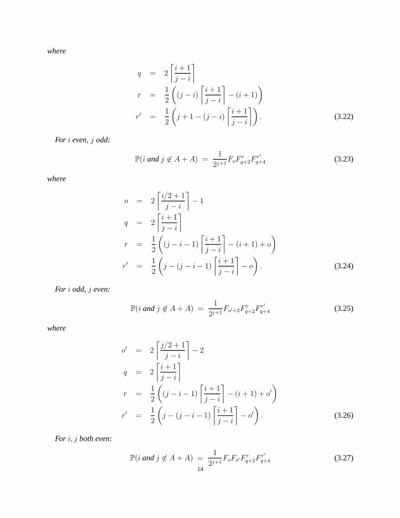
where
q = 2
⌈i+ 1
j − i
⌉
r =1
2
((j − i)
⌈i+ 1
j − i
⌉− (i+ 1)
)
r′ =1
2
(j + 1− (j − i)
⌈i+ 1
j − i
⌉). (3.22)
For i even,j odd:
P(i andj 6∈ A+ A) =1
2j+1FoF
rq+2F
r′
q+4 (3.23)
where
o = 2
⌈i/2 + 1
j − i
⌉− 1
q = 2
⌈i+ 1
j − i
⌉
r =1
2
((j − i− 1)
⌈i+ 1
j − i
⌉− (i+ 1) + o
)
r′ =1
2
(j − (j − i− 1)
⌈i+ 1
j − i
⌉− o
). (3.24)
For i odd,j even:
P(i andj 6∈ A+ A) =1
2j+1Fo′+2F
rq+2F
r′
q+4 (3.25)
where
o′ = 2
⌈j/2 + 1
j − i
⌉− 2
q = 2
⌈i+ 1
j − i
⌉
r =1
2
((j − i− 1)
⌈i+ 1
j − i
⌉− (i+ 1) + o′
)
r′ =1
2
(j − (j − i− 1)
⌈i+ 1
j − i
⌉− o′
). (3.26)
For i, j both even:
P(i andj 6∈ A+ A) =1
2j+1FoFo′F
rq+2F
r′
q+4 (3.27)14

where
o = 2
⌈i/2 + 1
j − i
⌉− 1
o′ = 2
⌈j/2 + 1
j − i
⌉− 2
q = 2
⌈i+ 1
j − i
⌉
r =1
2
((j − i− 2)
⌈i+ 1
j − i
⌉− (i+ 1) + o+ o′
)
r′ =1
2
(j − 1− (j − i− 2)
⌈i+ 1
j − i
⌉− o− o′
). (3.28)
We conclude this section with some bounds onP(i andj 6∈ A + A). We have (Binet’s formula)
Fn =1√5(φn − (−1/φ)n), (3.29)
whereφ = (1 +√5)/2 is the golden ratio. Therefore, for evenn we have
Fn ≤ 1√5φn. (3.30)
Sinceq + 2 andq + 4 are always even, then for anyi, j both odd, we have
P(i andj 6∈ A+ A) =1
2j+1F rq+2F
r′
q+4
≤ 1
2j+1
(φq+2
√5
)r (φq+4
√5
)r′
=1
2j+1
φ(qr+(q+2)r′)+(2r+2r′)
5(r+r′)/2
=1
2j+1
φj+1+j−i
5(j−i)/4
=φ2j+1
2j+15j/45i/4
φi, (3.31)
where the second to last equality comes from (3.18). In fact,we can use Proposition 3.5 to showthat (3.31) holds for alli, j (slightly better constants hold for the otheri, j).
If i = k andj = k +m, wherem is fixed andk goes to infinity, a lower bound similar to (3.31)also holds. First note that for evenn
F rn =
1
5r/2(φn − φ−n
)r
=1
5r/2φnr(1− φ−2n
)r
=1
5r/2φnr(1− r(1− c)r−1φ−2n
)(3.32)
15

for somec such that0 < c < 1/φ2n by Taylor expansion. Therefore for oddi, j, we have
P(i andj 6∈ A+ A) =1
2j+1F rq+2F
r′
q+4
≥ 1
2j+1
1
5(q+2)/2φ(q+2)r(1− rφ−2(q+2))
1
5(q+4)/2φ(q+4)r′(1− r′φ−2(q+4))
=φ2j+1
2j+15j/45i/4
φi(1− rφ−2(q+2))(1− r′φ−2(q+4))
≥ φ2j+1
2j+15j/45i/4
φi(1− (r + r′)φ−2(q+2))
≥ φ2j+1
2j+15j/45i/4
φi(1− (j − i)φ−i/(j−i)), (3.33)
and similar formulas hold for the other parity cases. Ifj/i → 1 not too slowly, then the remainderterm on the right-hand-side of (3.33) goes to1. For example, ifi = k andj = k + m, then wehave the following corollary by combining (3.31) and (3.33).
Corollary 3.6. For any fixedm,
P(k andk +m 6∈ A + A) ∼ φ2(k+m)+1
2(k+m)+15(k+m)/4
5k/4
φk=
φk+1
2k+1
φ2m
2m5m/4, (3.34)
ask goes to infinity withk, k +m are both odd. Similar asympotics hold for generalk, k +m. Ifwe ignore the constants related tom, we have
P(k andk +m 6∈ A + A) = Θ((φ/2)k) (3.35)
ask goes to infinity with anyk, k +m.
Note that sinceP(i andj 6∈ A + A) has exponential decay ini, j as seen in (3.31), then (3.11)converges asn → ∞; that is
limn→∞
Var(M[0,n−1](A)
)= 4
∑
i<j
P(i andj 6∈ A+ A)− 40 (3.36)
exists and is finite. In particular, we know that the limit is an infinite sum of Fibonacci products.However, we could not find a closed form for this sum. Nonetheless, because of the exponentialdecay in the terms in the sum, we can approximate the variancewell. In particular, note that thetail of the sum has exponential decay:
∑
n≤i<j
P (i andj 6∈ A+ A) ≤∑
n≤i<j
φ
2
(φ2
2 · 51/4)j (
51/4
φ
)i
≤ φ
2
(∑
n≤j
(φ2
2 · 51/4)j)(∑
n≤i
(51/4
φ
)i)
≤ φ
2
(1
1− φ2/2 · 51/4)(
1
1− 51/4/φ
)(φ2
2 · 51/4)n(
51/4
φ
)n
≤ 87
(φ
2
)n
≤ 87(0.81)n. (3.37)
16

Here we use that (3.31) holds for alli, j. Using Mathematica to sum the first300 terms of (3.36),whose exact form is given in Proposition 3.5, we get the following approximation for the variance:
limn→∞
Var(M[0,n−1](A)
)= 35.9658 + E, (3.38)
where|E| < 10−4. The error termE comes mostly from truncating the computation of the 300-term series given by Mathematica. By (3.37), the error term from truncating the series atn = 300is less than87(0.81)300 ∼ 3 · 10−28, which is much less than the Mathematica error term. Thisproves Theorem 1.5.
4. EXPONENTIAL BOUNDS
We now prove Theorem 1.2 and find exponential bounds for the distribution ofM[0,n−1](A).
Proof of Theorem 1.2.For the lower bound, we construct manyA such thatA + A is missingkelements. First suppose thatk is even. Let the firstk/2 non-negative integers not be inA. Thenlet the rest of the elements ofA be any subsetA′ that fills in (soA′ + A′ has no missing elementsbetween its largest and smallest elements); that isMn−k/2(A
′) = 0. By [MO, Proposition 8], wecan show that
P(M[0,n−1](A′) = 0) > 1/210 (4.1)
independent ofn. If L ⊆ [0, ℓ− 1] andU ⊆ [n − u, n − 1] are fixed, then their proposition saysthat
P([2ℓ−1, 2n−2u−1] ⊆ A′+A′ |A′∩[0, ℓ−1] = L,A′∩[n−u, n−1] = U) > 1−6(2−|L|+2−|U |),(4.2)
independent ofn. Therefore,
P([2ℓ− 1, 2n− 2u− 1] ⊆ A′ + A′ andA′ ∩ [0, ℓ− 1] = L,A′ ∩ [n− u, n− 1] = U)
> (1− 6(2−|L| + 2−|U |))2−ℓ2−u. (4.3)
By lettingL = [0, ℓ− 1], U = [n− u, n− 1] so the ends fill in, we get that
P(A′ + A′ = [0, 2n− 2]) > (1− 6(2−ℓ + 2−u))2−ℓ2−u. (4.4)
Letting ℓ = u = 4 so that the first term in the product is positive, we get that
P(A′ + A′ = [0, 2n− 2]) > (1− 6(2−4 + 2−4))2−42−4 = 1/210, (4.5)
independent ofn, which gives us (4.1).AsA = k/2 +A′, we haveA+A = k +A′ +A′ = [k, 2n− 2] and soM[0,n−1](A) = k as seen
by Figure 7.Therefore we have
P(M[0,n−1](A) = k) ≥ P(A = k/2 + A′ andMn−k/2(A′) = 0)
=
(1
2
)k/2
P(Mn−k/2(A′) = 0)
≫(1
2
)k/2
≥ (0.70)k, (4.6)
where the implied constants are independent ofn by (4.1). This proves the lower bound in Theorem1.2 whenk is even.
17

.
FIGURE 7. A andA+ A for lower bound.
If k is odd, then we can letL = [0, ℓ−1]\{2, 3} andU = [n−u, n−1] so that only the element3 is missing fromA′ + A′. Then we get a bound forP(M[0,n−1](A
′) = 1) as in (4.1). LettingA = (k − 1)/2 + A′, we get the desired lower bound in Theorem 1.2 for whenk is odd.
For the upper bound, we can use bounds like
P(k 6∈ A + A) ≤(3
4
)k/2
(4.7)
from [MO]. Again, first suppose thatk is even. Note that ifA+A is missingk elements, then oneof these missing elements must be at leastk/2 elements away from the ends of[0, 2n− 2]. That is,we have the following situation (see Figure 8).
FIGURE 8. Upper bound forP(M[0,n−1](A) = k)
Therefore
P(M[0,n−1](A) = k) ≤ P(A + A missing element at leastk/2 away from edges)
= P(j 6∈ A+ A, j ∈ [k/2, 2n− k/2])
≤ 2∑
j≥k/2
(3
4
)j/2
≪(3
4
)k/4
≈ (0.93)k. (4.8)
Note that this bound does not use the fact that there may be missing elements on both ends atthe same time. By focusing on one particular side, we can get astronger result. For example, we
18

have the following inequality for the probability of missing k elements in[0, n/2]:
P(|[0, n/2] \ (A+ A)| = k) ≤ P(j 6∈ A + A, j ∈ [k, n/2])
≤ 2∑
j≥k
(3
4
)j/2
≪(3
4
)k/2
≈ (0.87)k (4.9)
and similarly forP(|[3n/2, 2n] \ (A+ A)| = k). Furthermore, (7.27) from Section 7 connects theprobability of missingk elements to the probability of missing elements in[0, n/2] and[3n/2, 2n]:
P(M[0,n−1](A) = k) =∑
i+j=k
P(|[0, n/2]\(A+A)| = i)P(|[3n/2, 2n]\(A+A)| = j)+O
((3
4
)n/4).
(4.10)Combining (4.9) and (4.10), we get
P(M[0,n−1](A) = k)
=∑
i+j=k
P(|[0, n/2] \ (A+ A)| = i)P(|[3n/2, 2n] \ (A+ A)| = j) +O
((3
4
)n/4)
≪∑
i+j=k
(3
4
)i/2(3
4
)j/2
+
(3
4
)n/4
≪ k
(3
4
)k/2
+
(3
4
)n/4
. (4.11)
Therefore ifk/2 < n/4, then we get the desired bound
P(M[0,n−1](A) = k) ≪ k
(3
4
)k/2
≈ (0.87)k. (4.12)
Note that the bound in (4.12) for the distribution is exactlythe same as the bound in (4.9) formissing elements on a single side. Since all our bounds are exponential and (4.10) multipliesP(|[0, n/2] \ (A + A)| = i) with P(|[3n/2, 2n] \ (A + A)| = j), we can always use this approachto transform bounds on the probability of missing elements in (A + A) ∩ [0, n/2] to equally goodbounds on number of missing elements in all ofA + A. So it is sufficient to just develop boundson missing elements on one side ofA+A. In particular, we can use this approach to transform the
19

bounds in Corollary 3.6 to improve the bounds in (4.12). By Corollary 3.6, we have
P(|[0, n/2] \ (A+ A)| = k) ≤ P(A+ A misses 2 elements greater thank − 3)
= P(i, j 6∈ A+ A, i, j ∈ [k − 3, n/2])
=∑
k−3<i<j
P(i andj 6∈ A + A)
≪∑
k−3<i<j
φ2j+1
2j+15j/45i/4
φi
≪ φ2k+1
2k+15k/45k/4
φk=
(φ
2
)k
≈ (0.81)k. (4.13)
Then using the previous approach, we get a similar bound on the total number of missing sums:
P(M[0,n−1](A) = k) ≪(φ
2
)k
≈ (0.81)k. (4.14)
Note that as in (4.10), we always have an extra(3/4)n/4 term. To make this term negligible,we need to have(3/4)n/4 < (0.81)k, which meansn > k · 4 log(0.81)/ log(3/4) ∼ 2.92k or thatk < 0.34n. This condition is sufficient in this case where we have the bound(φ/2)k. However ingeneral, we know that we have a lower bound of(1/2)k/2 for the distribution. Therefore, to makethe(3/4)n/4 term always negligible, we can have(3/4)n/4 < (1/2)k/2, which meansn > k · 2 log(1/2)/ log(3/4) ∼ 5k, as in the statement of Theorem 1.2. Note that then the impliedconstants are independent ofn. Combining (4.6) and (4.14), we get Theorem 1.2. �
5. APPROXIMATING P(k + a1, k + a2, . . . , AND k + am 6∈ A+ A)
In this section, we prove Theorem 1.6 which says that for any fixed a1, . . . , am, there existsλa1,...,am such that
P(k + a1, k + a2, . . . , andk + am 6∈ A + A) = Θ(λka1,...,am
), (5.1)
where the implied constants depend ona1, . . . , am but notk. Therefore, the probability is approx-imately exponential.
To prove this theorem, we use a version of Fekete’s Lemma, which says that sub-additive se-quences are approximately linear. From [S] we have the following version in which the sequenceis both sub-additive and super-additive.
Lemma 5.1. If bn is a sequence such that
bn + bm − 1 ≤ bn+m ≤ bn + bm + 1 (5.2)
for all n,m, thenλ = inf bn/n exists and for alln,∣∣∣∣bnn
− λ
∣∣∣∣ <1
n. (5.3)
Remark 5.2. The proof of this Lemma can be easily modified to get that if
bn + bm − c ≤ bn+m ≤ bn + bm + c (5.4)20
for some constantc > 0, then ∣∣∣∣bnn
− λ
∣∣∣∣ <c
n. (5.5)
Suppose thatan is approximately multiplicative rather than approximately additive so that forsome constantc > 1
c−1 · aman ≤ am+n ≤ c · aman (5.6)
for all m,n. As bn = log an satisfies the properties of Lemma 5.1, forλ = inf log ann
we have∣∣∣∣log ann
− λ
∣∣∣∣ <log c
n(5.7)
for all n. That is,c−1λn ≤ an ≤ cλn (5.8)
for all n, implying
an = Θ(λn). (5.9)
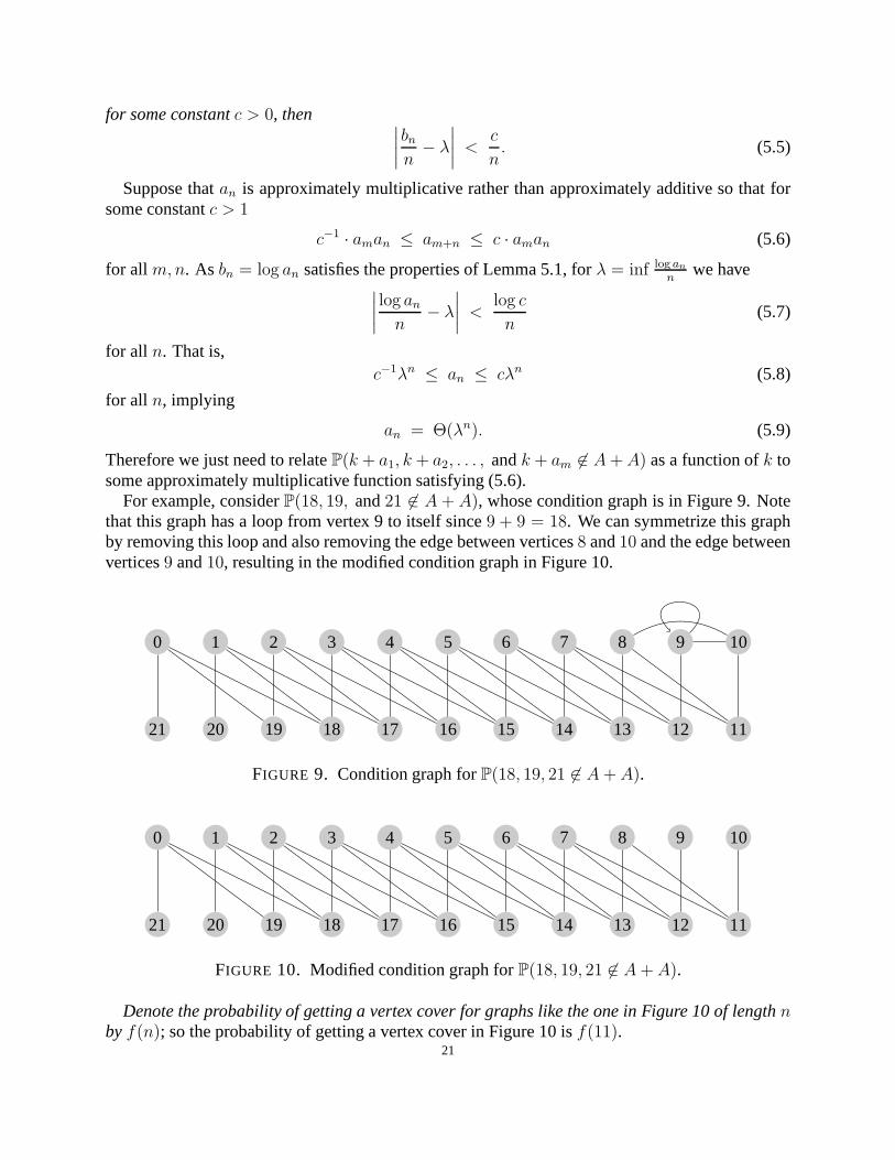
Therefore we just need to relateP(k + a1, k + a2, . . . , andk + am 6∈ A+A) as a function ofk tosome approximately multiplicative function satisfying (5.6).
For example, considerP(18, 19, and21 6∈ A + A), whose condition graph is in Figure 9. Notethat this graph has a loop from vertex 9 to itself since9 + 9 = 18. We can symmetrize this graphby removing this loop and also removing the edge between vertices8 and10 and the edge betweenvertices9 and10, resulting in the modified condition graph in Figure 10.
0 1 2 3 4 5 6 7 8 9 10
21 20 19 18 17 16 15 14 13 12 11
FIGURE 9. Condition graph forP(18, 19, 21 6∈ A+ A).
0 1 2 3 4 5 6 7 8 9 10
21 20 19 18 17 16 15 14 13 12 11
FIGURE 10. Modified condition graph forP(18, 19, 21 6∈ A+ A).
Denote the probability of getting a vertex cover for graphs like the one in Figure 10 of lengthnbyf(n); so the probability of getting a vertex cover in Figure 10 isf(11).
21

Note thatf(11) is an upper bound for the probability in the original condition graph in Figure 9since we have removed some edges. On the other hand, we have the following lower bound:
P(18, 19, and21 6∈ A + A)
≥ P(18, 19, 21 6∈ A+ A and9, 10, 11, 12 6∈ A)
= P(18, 19, 21 6∈ A+ A | 9, 10, 11, 12 6∈ A)P(9, 10, 11, 12 6∈ A). (5.10)
Note that the condition graph forP(18, 19, 21 6∈ A+A | 9, 10, 11, 12 6∈ A) is the original conditiongraph in Figure 9 with all edges incident on vertices9, 10, 11 or 12 removed, as depicted in Figure11.
0 1 2 3 4 5 6 7 8
21 20 19 18 17 16 15 14 13
FIGURE 11. Condition graph forP(18, 19, and21 6∈ A+ A | 9, 10, 11, 12 6∈ A).
Note that in Figure 11 we have removed vertices9, 10, 11 and12 completely since there are nolonger any conditions on them inP(18, 19, and21 6∈ A+A | 9, 10, 11, 12 6∈ A). Finally, note thatthe probability of getting a vertex cover in the graph in Figure 11 is justf(9). Therefore, by (5.10),we have
(1/2)4f(9) ≤ P(18, 19, and21 6∈ A+ A) ≤ f(11), (5.11)
where we use thatP(9, 10, 11, 12 6∈ A) = (1/2)4.Since the condition graph forP(k, k + 1, andk + 3 6∈ A + A) is just a longer version of the
condition graph forP(18, 19, and21 6∈ A + A), we can apply the same method as before to getthat
(1/2)4f(k/2) ≤ P(k, k + 1, andk + 3 6∈ A+ A) ≤ f((k + 4)/2) (5.12)
for evenk, with a similar formula holding for oddk. Therefore we are reduced to studyingf(n),which is easier to investigate since the condition graph is more symmetric. We will show thatf(n)satisfies (5.6), implying it is approximately exponential.
For example, to see thatf(11) ≤ f(4)f(7), we can separate the graph in Figure 10 at the4th
vertex and remove edges that cross this gap, resulting in thegraph in Figure 12.
0 1 2 3 4 5 6 7 8 9 10
21 20 19 18 17 16 15 14 13 12 11
FIGURE 12. Upper Bound forf(11).
Since the components are independent smaller copies of the original, the probability of gettinga vertex cover for the graph in Figure 12 isf(4)f(7). We can do this for any integer less than
22

11, definingf(n) for small integers by truncating at thenth vertex. Since we have removed someedges to get the graph in Figure 12, we have
f(11) ≤ f(4)f(7) (5.13)
as desired.To get a lower bound forf(11), we use that
f(11) ≥ f(11 | 4, 5, 6, 15, 16, 17 chosen)P(4, 5, 6, 15, 16, 17 chosen), (5.14)
wheref(11 | 4, 5, 6, 15, 16, 17 chosen) denotes the probability of getting a vertex cover for thegraph in Figure 12 given that the vertices4, 5, 6, 15, 16, 17 are chosen. The graph forf(11 |4, 5, 6, 15, 16, 17 chosen) is depicted in Figure 13. The probability of getting vertex covers for the
0 1 2 3 4 5 6 7 8 9 10
21 20 19 18 17 16 15 14 13 12 11
FIGURE 13. Lower Bound forf(11).
two independent components isf(4)f(4). Therefore from (5.14), we get that
f(11) ≥ (1/2)6f(4)f(4) ≥ (1/2)6f(4)f(7), (5.15)
with the last inequality sincef(n) is decreasing. Therefore, in general we have
(1/2)6f(m)f(n) ≤ f(m+ n) ≤ f(m)f(n), (5.16)
and sof(n) satisfies the conditions of (5.6). By the modified version of Fekete’s Lemma, we have
f(n) = Θ(λn) (5.17)
for someλ. Therefore by (5.12), we have
P(k, k + 1, andk + 3 6∈ A+ A) = Θ(λk/2), (5.18)
which proves Theorem 1.6 for the casea1 = 0, a2 = 1, a3 = 3.The general situation follows in exactly the same way: by first making the configuration graph
of P(k+a1, . . . , andk+am 6∈ A+A) look more symmetric and then using the modified Fekete’sLemma.
6. CONSECUTIVE M ISSING SUMS
In this section, we prove Theorem 1.7 and its generalizationTheorem 1.8. We begin by provingTheorem 1.7, which says that
(1
2
)(k+m)/2
≪ P(k + 1, . . . , andk +m 6∈ A+ A) ≪(1
2
)(k+m)/2
(1 + ǫm)k. (6.1)
23

The lower bound comes from the construction in Figure 7 by letting the first⌊(k+m)/2⌋ elementsof A be missing, which forces the firstk +m elements ofA + A to be missing as well. That is,
P(0, 1, . . . , k +m− 1, andk +m 6∈ A+ A)
= P(0, 1, . . . , and⌊(k +m)/2⌋ 6∈ A)
= (1/2)⌊(k+m)/2⌋+1. (6.2)
Therefore, we only need to prove the upper bound.Before giving the proof, we consider an example with condition graphs which illustrates the
idea. ConsiderP(16, 17, 18, 19, 20 6∈ A+ A). The condition graph here is given in Figure 14.
0 1 2 3 4 5 6 7 8
20 19 18 17 16 15 14 13 12 11 10 9
FIGURE 14. Condition graph forP(16, 17, 18, 19, 20 6∈ A + A).
We need to find the probability of getting a vertex cover for this graph. If we remove someedges, the probability of getting a vertex cover for the resulting graph is an upper bound for theprobability of getting a vertex cover for the original graph. We can remove some edges to get thegraph of Figure 15.
0 1 2 3 4 5 6 7 8
20 19 18 17 16 15 14 13 12 11 10 9
FIGURE 15. Graph after removing some edges.
The resulting graph has3 ∼ 20/6 components that are all complete bipartite graphs with6vertices. These are easier to handle since the only way to geta vertex cover for such graphs is tohave all vertices on one side be chosen. So the probability ofgetting a vertex cover for one of thesecomplete bipartite components is less than(1/2)3+(1/2)3 = 2/23. Since the components are alsoindependent, we have
P(16, 17, 18, 19, 20 6∈ A + A) ≤(
2
23
)3
∼(1
4
)20/6
. (6.3)
and in general we get that
P(k, k + 1, k + 2, k + 3, k + 4 6∈ A+ A) ≤(
2
23
)(k+4)/6
=
(21/3
2
)(k+4)/2
. (6.4)
24

We use this approach in the general proof. Notice that asm → ∞, the size of the complete bipar-tite graphs grows, and so we will be taking out relatively fewer and fewer constraints. Therefore,this approach gets us closer to the correct answer.
Now we give a formal proof of Theorem 1.7 that does not rely on the condition graphs.
Proof. We first do the proof forP(k, k + 1, . . . , andk + 2m − 1 6∈ A + A) with 2m − 1 insteadof m. Note that since the probability depends only on[0, k + 2m − 1] ∩ A, we can assume thatA ⊆ [0, k + 2m− 1]. We will also assume thatm dividesk and that
k = qm (6.5)
with q even.We begin by writingA as the following disjoint union:
A = A0 ∪A1 ∪ · · · ∪ Aq ∪ Aq+1, (6.6)
whereAj = A ∩ [jm, (j + 1)m− 1]. (6.7)
Then if [k, k+2m− 1]∩ (A+A) = ∅, then[k, k+2m− 1]∩ (Aj +Aq−j) = ∅ for all j. Note that
Aj + Aq−j ⊆ [k, k + 2m− 2]. (6.8)
Therefore,[k, k + 2m− 1] ∩ (Aj + Aq−j) = ∅ impliesAj + Aq−j = ∅. If q is even, we have
P(k, k + 1, . . . , andk + 2m− 1 6∈ A + A) < P([k, k + 2m] ∩ (Aj + Aq−j) = ∅ for all j ≤ q/2)
= P(Aj + Aq−j = ∅ for all j ≤ q/2)
= P(Aj = ∅ orAq−j = ∅ for all j ≤ q/2). (6.9)
For differentj, the pairs of setsAj , Aq−j are disjoint. Therefore, we have independence:
P(Aj = ∅ orAq−j = ∅ for all j ≤ q/2) = P(Aq/2 = ∅)q/2−1∏
j=0
P(Aj = ∅ orAq−j = ∅). (6.10)
Finally, note that
P(Aj = ∅ orAq−j = ∅) ≤ P(Aj = ∅) + P(Aq−j = ∅) = 2
2m. (6.11)
Combining (6.9), (6.10), and (6.11), we find
P(k, k + 1, . . . , andk + 2m− 1 6∈ A+ A) ≤ 1
2m
q/2−1∏
j=0
2
2m
= 2q/2(
1
2m
)q/2+1
= 2k/2m(1
2
)(k+2m)/2
. (6.12)
This inequality is true for allm, k such thatq = k/m is an even integer.Changingm to m/2, we get that
P(k, k + 1, . . . , andk +m− 1 6∈ A+ A) ≤ 2k/m(1
2
)(k+m)/2
(6.13)
25

for evenm andq = k/m still an even integer. Note that (6.13) is similar to the bound we get in(6.4) using the condition graph approach.
For oddm, we just need to use (6.13), noting that
P(k, k+1, . . . , k+m−1, andk+m 6∈ A+A) ≤ P(k, k+1, . . . , andk+m−1 6∈ A+A). (6.14)
For oddq, we need to partitionA such that there is a block in the very middle ofA. This ensuresthat this middle block is matched with itself (just likeAq/2 was matched with itself whenq waseven). This gives us the extra1/2m that is needed in order to achieve the bound. For non-integerq, we need to repartitionA in a similar way. Therefore the bound in (6.13) holds in general, up toa constant.
Finally, note that asm → ∞, we have21/m → 1. Writing 21/m = 1 + ǫm, we have
P(k, . . . , andk +m− 1 6∈ A+ A) <
(1
2
)(k+m)/2
(1 + ǫm)k, (6.15)
whereǫm → 0 asm → ∞. By raising21/m = 1 + ǫm to themth power, we see that
ǫm <1
m. (6.16)
Therefore a weakened version of the inequality says that(1
2
)(k+m)/2
≪ P(k + 1, . . . , andk +m 6∈ A+ A) ≪(1
2
)(k+m)/2
(1 + ǫm)k, (6.17)
where the implied constants are independent ofm andk.This bound is interesting since it means that the trivial lower bound is almost the right answer
for the exact bound. The trivial lower bound makes us miss allof [0, k +m] in A + A as seen in(6.2) but we only need[k + 1, k +m] to be missing. In this sense, we see that essentially the onlyway to missm consecutive elements atk + 1 for largem is to miss all the previous elements aswell.
Also, note that (6.17) implies that
λ0,1,...,m →(1
2
)1/2
(6.18)
asm → ∞ by definition ofλ0,1,...,m. �
Now we will prove Theorem 1.8, which says that
λa1,...,am ≤ P(A,B ⊆ [0, ⌊am/2⌋] | a1, . . . , am 6∈ A+ B)1/(am+2). (6.19)
Note that Theorem 1.7 is indeed a special case of this theoremsince we have the following upperbound
λ0,1,...,m ≤ P(A,B ⊆ [0, ⌊m/2⌋] | 0, . . . , m 6∈ A+B)1/(m+2)
= P(A,B ⊆ [0, ⌊m/2⌋] | A = ∅ orB = ∅)1/(m+2)
≤(2
(1
2
)⌊m/2⌋+1)1/(m+2)
, (6.20)
which converges to√
1/2.The proof of Theorem 1.8 will be almost exactly the same as theproof of Theorem 1.7.
26

Proof. We will first show that for0 ≤ a1 < · · · < am,
P(A ⊆ [0, k + am] | k + a1, . . . , k + am 6∈ A+ A)
≤ P(A,B ⊆ [0, am/2] | a1, . . . , am 6∈ A +B)k/(am+2) (6.21)
for all k, am such thatam is even andam + 2 dividesk. Similar results hold in the other cases ofk,m. Furthermore, we first assume thatam = 2r− 2. Note that since the probability depends onlyon [0, k + 2r − 2] ∩ A, we can takeA ⊆ [0, k + 2r − 2]. Again, we first assume thatr divideskand thatk = qr. Then as before,
P(k + a1, . . . , andk + am 6∈ A+ A)
≤ P(k + a1, . . . , andk + am 6∈ Aj + Aq−j for all j ≤ ⌊q/2⌋)
=
⌊q/2⌋∏
j=0
P(k + a1, . . . , andk + am 6∈ Aj + Aq−j). (6.22)
The key fact is that ifj 6= q − j, the setsAj , Aq−j are independent and
P(k + a1, . . . , andk + am 6∈ Aj +Aq−j) = P(A,B ⊆ [0, r− 1] | a1, . . . , am 6∈ A+B) (6.23)
for all j. Therefore, ifq is odd
P(k + a1, . . . , andk + am 6∈ A + A)
≤ P(A,B ⊆ [0, r − 1] | a1, . . . , am 6∈ A+B)⌊q/2⌋+1
= P(A,B ⊆ [0, r − 1] | a1, . . . , am 6∈ A+B)k/2r+1/2 (6.24)
and if q is even,
P(k + a1, . . . , andk + am 6∈ A+ A)
≤ P(A ⊆ [0, r − 1] | a1, . . . , am 6∈ A+ A)
× P(A,B ⊆ [0, r − 1] | a1, . . . , am 6∈ A+B)k/2r. (6.25)
If we drop the terms that do not depend onk, we have for all evenam and allk divisible byam +2
P(A ⊆ [0, k + am] | k + a1, . . . , k + am 6∈ A + A)
≤ P(A,B ⊆ [0, am/2] | a1, . . . , am 6∈ A+B)k/(am+2), (6.26)
which is (6.21). Note that ifk is not divisible byam + 2 or if am is not even, we have
P(A ⊆ [0, k + am] | k + a1, . . . , k + am 6∈ A+ A)
≤ P(A,B ⊆ [0, ⌊am/2⌋] | a1, . . . , am 6∈ A+B)⌊k/(am+2)⌋, (6.27)
which proves that (6.19).�
7. BOUNDS ONm(k), w(k), y(k), AND z(k) FOR k < 32
As mentioned in §1.3 and covered in more detail in §7.2, it suffices to boundz(k). Our strategyis this: ifD +D (whereD is a uniformly chosen subset ofN that contains 0) is missing exactly 7elements, then it is very likely that those 7 missing sums areall smaller than 88 and typically evenall smaller than 44. If we loop over all243 possibilitiesβ for D∩[0, 44), for each possibility we cancompute(D+D)∩[0, 44) = (β+β)∩[0, 44) and a subset of(D+D)∩[44, 48) ⊇ (β+β)∩[44, 88).From this (with a little theory to handle the tail of the sumset) we can bound the likelihood of
27

missing exactly 7 sums, givenD ∩ [0, 44). By combining these estimates, we acquire bounds onz(7).
Let n ≥ 2 be a natural number parameter (the computations reported here usen = 44, althoughn = 43 is already enough to showm(7) < m(6) < m(8)), and set
z(k | β) := P (|N \ (D +D)| = k | D ∩ [0, n) = β) . (7.1)
We have
z(k) =∑
0∈β⊆[0,n)
z(k | β)P (D ∩ [0, n) = β) = 2−(n−1)∑
0∈β⊆[0,n)
z(k | β), (7.2)
so that it suffices to boundz(k | β) above and below for all0 ≤ k < 32 (our arbitrary notion of“small k” is 0 ≤ k < 32) and all0 ∈ β ⊆ [0, n).
Further, set
B := D ∩ [0, n)
D := [0, n) \ (β + β)
L := [n, 2n) \ (β + β)
m := minLT := [2n,∞)
η := E [|[n,∞) \ (D +D) | B = β]
µ := 2−|β∩[0,m−n]|. (7.3)
If we condition onB = β, then the elements ofD areDefinitely missing fromD + D, theelements ofL areLikely but not certain to be missing, and the elements ofT , theT ail of thenatural numbers, are very likely to be missing. Note that2n − 1 ∈ L, soL is nonempty andm iswell-defined.
Lemma 7.1. For all k < |D|, we havez(k | β) = 0.
Proof. Conditioning onB = β, we haveD ⊆ N \ (D +D). In fact,D = [0, n) \ (D +D). �
Lemma 7.2. We haveη = 5 · 2−|B| +∑
ℓ∈L
2−|B∩[0,ℓ−n]|.
Proof. By linearity of expectation
η := E [|[n,∞) \ (D +D)|] = E [|[n, 2n) \ (D +D)|] + E [|T \ (D +D)|] . (7.4)
Again using linearity of expectation, we have
E [|[n, 2n) \ (D +D)|] =∑
ℓ∈L
P (ℓ 6∈ D +D) (7.5)
Sinceℓ 6∈ D +D is the same as (forn ≤ ℓ < 2n)
ℓ 6∈ D +D =
ℓ/2∧
i=0
(i 6∈ D ∨ ℓ− i 6∈ D)
=∧
b∈βb≤ℓ−n
ℓ− b 6∈ D. (7.6)
28

ThusP (ℓ 6∈ D +D) = 2−|β∩[0,ℓ−n]|, (7.7)
and so ∑
ℓ∈L
P (ℓ 6∈ D +D) =∑
ℓ∈L
2−|β∩[0,ℓ−n]|. (7.8)
ThatE [|T \ (D +D)|] = 5 · 2−|β| (7.9)
is essentially in [MO], but we derive it here for the reader’sconvenience. Using linearity of expec-tation,
E [|T \ (D +D)|] =∞∑
t=2n
P (t 6∈ D +D) (7.10)
and
P (t 6∈ D +D) = P
(∧
b∈β
t− b 6∈ D
)∧
t/2∧
i=n
i 6∈ D ∨ t− i 6∈ D
. (7.11)
Now this has two cases leading to
P (t 6∈ D +D) =
{2−|β|(3/4)(t−2n+1)/2 t is odd,
2−|β|(1/2)(3/4)(t−2n)/2 t is even.(7.12)
The infinite sum (7.10) now simplifies5 · 2−|β|. �
Lemma 7.3. We havemax{0, 1− η} ≤ z(|D| | β) ≤ 1− µ.
Proof. Trivially z(|D| | β) ≥ 0. Since
η = E [|[n,∞) \ (D +D)| | B = β]
=∞∑
i=0
z(|D|+ i | β) · i
≥∞∑
i=1
z(|D|+ i | β)
= 1− z(|D| | β), (7.13)
we also havez(|D| | β) ≥ 1− η.Observe that the event|N \ (D +D)| > |D| contains the event{m 6∈ D +D}, and so
P (|N \ (D +D)| = |D|) ≤ 1− P (m 6∈ D +D) = 1− µ, (7.14)
concluding the proof of this lemma. �
Lemma 7.4. We havemax{0, 2µ− η} ≤ z(|D|+ 1 | β) ≤ min{1, η}.Proof. Trivially 0 ≤ z(|D|+ 1 | β) ≤ 1. We have
η =∞∑
k=0
k · z(|D|+ k | β) ≥ z(|D|+ 1 | β), (7.15)
which leaves only the bound2µ− η ≤ z(|D|+ 1 | β) to prove.29

The idea here is that if exactly|D| + 1 sums are missing, they are very likely to be the|D|elements ofD, andm. Formally,
{|N \ (D +D)| = |D|+ 1} ⊇ {m 6∈ D +D} ∩⋂
ℓ∈Lℓ>m
{ℓ ∈ D +D} ∩⋂
t∈T
{t ∈ D +D}
⊇ {m 6∈ D +D} \
⋃
ℓ∈Lℓ>m
{ℓ 6∈ D +D} ∪⋃
t∈T
{t 6∈ D +D}
and so
z(|D|+ 1 | β) ≥ P (m 6∈ D +D)−∑
ℓ∈Lℓ>m
P (ℓ 6∈ D +D)−∑
t∈T
P (t 6∈ D +D)
= 2P (m 6∈ D +D)−∑
i∈L∪T
P (i 6∈ D +D)
= 2µ− η. (7.16)
�
Lemma 7.5. For k ≥ 2, 0 ≤ z(|D|+ k | β) ≤ 1
kmin{η, 2η − 2µ}.
We note that sometimes this bound is weaker thanz(|D|+ k | β) ≤ 1. This happens for fewenoughβ that, from a computational vantage point, it is not worth checking for.
Proof. Trivially, 0 ≤ z(|D|+ k | β). We have
η =
∞∑
i=0
i · z(|D|+ i) ≥ kz(|D|+ k), (7.17)
whencez(|D|+ k) ≤ η/k. But also,
η =
∞∑
i=0
i · z(|D|+ i)
= z(|D|+ 1) +∞∑
i=2
i · z(|D|+ i)
≥ 2µ− η + kz(|D|+ k), (7.18)
and soz(|D|+ k) ≥ (2η − 2µ)/k. �
30

7.1. Making the computation feasible, reliable, and verifiable.A massive computation hasbeen performed, so some words are necessary as to how this is feasible. Set
LOWER(k | β) :=
max{0, 2n − 2nη}, k = |D|max{0, 2 · 2nµ− 2nη}, k = |D|+ 1
0, otherwise
UPPER(k | β) :=
2n − 2nµ, k = |D|min{2n, 2nη}, k = |D|+ 1
0, otherwise
OVERHANG(k|β) :=
{min{2nη, 2 · 2nη − 2 · 2nµ}, k = |D|0, otherwise.
(7.19)
The lemmas above imply that that the vector
22n−1〈z(0), z(1), . . . , z(31)〉 =∑
0∈β⊆[0,n)
2n〈z(0 | β), z(1 | β), . . . , z(31 | β)〉 (7.20)
is bounded below componentwise by∑
0∈β⊆[0,n)
〈LOWER(0 | β), LOWER(1 | β), . . . , LOWER(31 | β)〉 (7.21)
and is bounded above componentwise by
∑
0∈β⊆[0,n)
(〈UPPER(0 | β),UPPER(1 | β), . . . ,UPPER(31 | β)〉+
〈OVERHANG(0 | β),OVERHANG(1 | β), . . . ,OVERHANG(31 | β)〉 ·M),
whereM is the32 × 32 matrix whose(i, j)th entry (running the indices from 0 to 31) is1j−i
ifj ≥ i+ 2, and is 0 otherwise. This allows us to compute an upper bound on z(0), . . . , z(31) from
∑
0∈β⊆[0,n)
〈UPPER(0 | β),UPPER(1 | β), . . . ,UPPER(31 | β)〉 (7.22)
and∑
0∈β⊆[0,n)
〈OVERHANG(0 | β),OVERHANG(1 | β), . . . ,OVERHANG(31 | β)〉. (7.23)
Observe that LOWER, UPPERand Overhang are always integral, as2nµ and2nη are both integers;this means that we can compute (7.21), (7.22) and (7.23) using only integer arithmetic.
We need to computeβ + β andβ ∩ [0, k] (for variousk) for eachβ. This work can be tremen-dously reduced by using a Gray code. That is, the subsets of[1, n) can be enumerated in sucha way that each set differs from its predecessor in only one element (either put in or taken out).By storing the representation function forβ + β (that is, the number of times each sum can bewritten as a sum of two elements ofβ), we can simply update the necessary computations insteadof re-computing.
31

Unfortunately, the size of the computation requires us to use2n+1-bit integers, and this is not asupported data type in most languages forn ≥ 32. The options of using C with GMP, Mathematica,or some other route to arbitrary size integers is prohibitedby the size of our computation and themodesty of our actual needs (we add, but never multiply, and know a priori the number of bitswe will need). Therefore, we choose to represent our numbersas arrays of 64-bit integers in C++(each element of the array represents a separate digit of thebinary expansion of the number, butthe digits aren’t restricted to{0, 1}). To further extend our reach, we ran the code on the parallelcomputing cluster at the High Performance Computing Cluster at the City University of New York.To facilitate parallelization, we breakβ into β1 = β ∩ [0, n1) andβ2 = β ∩ [n1, n). This makesthe algorithm “embarrassingly parallel”, and allows us to store intermediate calculations both torecover from any system or power failings, and to allow for spot checking of results.
To ensure correctness of the results, we have written the code in Mathematica using the simplestalgorithms conceivable. Such code becomes intractably slow aroundn ≈ 25, but this provides asequence of values against which we can test our progressively more subtly written code, both inMathematica and in C++. Our most sophisticated code is in C++.
Finally, we have the bounds onP (|N \ (D +D)| = k | D ∩ [0, 210) = β1) for all β1 in a pub-licly available file, together with our source code. We invite the reader to spot check our imple-mentation.
7.2. Obtaining y(k), m(k), and w(k) from z(k). While it is clear thatz(k) is defined, thatis, the event “|N \ (D + D)| = k” is measurable, it is less clear thatz(∞) = 0. This, and thaty(∞) = 0, follows from the Borel-Cantelli lemma and bounds such as (1.10). We can defineD (auniformly chosen subset ofN containing 0) asC −minC (whereC is a uniformly chosen subsetof N), and so
y(k) =
∞∑
i=0
P (minC = i AND |N \ (C + C)| = k)
=∞∑
i=0
P (minC = i AND |N \ ((C −minC) + (C −minC))| = k − 2i)
=
⌊k/2⌋∑
i=0
P (minC = i)P (|N \ (D +D)| = k − 2i)
=
⌊k/2⌋∑
i=0
1
2i+1z(k − 2i). (7.24)
To obtain the formulas
m(k) =k∑
i=0
y(i)y(k − i), w(k) =k∑
i=0
z(i)z(k − i) (7.25)
32

we refer the reader to [I]. The gist of the argument is that
m(k) := P (|[0, 2n− 2] \ (A+ A)| = k)
=
k∑
i=0
P (|[0, n/2) \ (A + A)| = i AND |(3n/2, 2n− 2] \ A+ A| = k − i)
+ P (A+ A misses an element in[n/2, 3n/2])
=k∑
i=0
P (|[0, n/2) \ (A + A)| = i AND |(3n/2, 2n− 2] \ A+ A| = k − i) +O
((3
4
)n/4).
(7.26)
SinceA+A∩ [0, n/2) is only affected byA∩ [0, n/2) andA+A∩ (3n/2, 2n−2] is only affectedby A ∩ (n/2, n), we can use independence to write
m(k) =
k∑
i=0
P (|[0, n/2) \ (A + A)| = i) P (|(3n/2, 2n− 2] \ A+ A| = k − i)+O
((3
4
)n/4).
(7.27)so that
m(k) ∼k∑
i=0
P (|[0, n/2) \ (A+ A)| = i) P (|(3n/2, 2n− 2] \ A+ A| = k − i) . (7.28)
As n → ∞, the set[0, n/2) \ (A+ A) looks more and more likeN \ (C + C), so that
P (|[0, n/2) \ (A+ A)| = i) → y(i), (7.29)
and similarly (after replacingA with n − 1 − A) for P (|(3n/2, 2n− 2] \ A + A| = k − i). Theargument forw(k) is identical, but with “D” in place “C”.
LetZ1, Z2 be independent random variables with the same distributionasMN|{0}, and setW :=
Z1 + Z2. ThenP (W = k) =∑k
i=0 z(i)z(k − i) = w(k), whence∑∞
i=0w(i) = 1, and similarly∑∞i=0m(i) = 1.Sincey(k) is a linear combination ofz(0), . . . , z(k) with positivecoefficients, the lower bounds
on z(0), . . . , z(k) immediately give a lower bound ony(k), and likewise upper bounds onz(0),. . . , z(k) yield an upper bound ony(k). The situation is the same betweeny andm and betweenzandw, even though the combination is not linear!
To experimentally estimatez(k), we hypothesized thatP (N \ (D +D) 6⊆ [0, 256)) is suffi-ciently small as to be ignored. Then, using Mathematica 8, wegenerated228 pseudorandom subsetsE of [0, 256), forced each to contain 0, and then computedk := |[0, 256) \ (E + E)| and kept arunning tally of the number of times each value ofk arose. This estimates (with an enormoussample size)
P (|N \ (D +D)| = k | N \ (D +D) ⊆ [0, 256)) ≈ z(k). (7.30)
The estimatesz(k), along with conservative 99.9% confidence intervals, are given in Table 16and shown in Figure 2. The implied bounds onw, m, andy are given in Tables 17, 18, and 19respectively, and shown in Figure 2.
33

8. CONJECTURES ANDFUTURE RESEARCH
We end with some conjectures that are supported by numericaldata. Our main conjecture re-mains Conjecture 1.3, which says that the distribution of missing sums is approximately expo-nential. One possible method of studying this distributionis finding where the first present sumin A + A occurs, given thatA + A hask missing elements. Recall that the lower bound in §4was proven by constructingA such thatM[0,n−1](A) = k by letting the firstk/2 elements ofAbe missing. In this case, the index of the first present sum inA + A occurs at indexk. But fromnumerical data, the index of the first present element will not bek for typicalA+A that is missingk elements. This also suggests that this trivial construction does not account for the real ‘random’way of constructingA such thatA+A is missingk elements, which is consistent with the fact thatthe conjectured decay constant for the distribution is approximately0.78 but the lower bound givesonly the decay constant approximately0.70. Even though the index of the first present element isnotk, from numerical data, the index seems to be linear ink.
To be precise, letXn(A) = max{m : if ℓ < m then ℓ 6∈ A+ A}
be the index of the first present sum ofA + A. Then we have the following conjecture.
Conjecture 8.1. For largek,
limn→∞
E(Xn(A) | M[0,n−1](A) = k) (8.1)
is asymptotically linear ink.
Similarly, we can investigate how far we must move to the right of zero and to the left of themaximum possible sum,2n− 2, so that there are no missing sums ofA+A in this interval. GivenA ∈ [0, n − 1] missing exactlyk sums, asn → ∞ each of thek missing elements ofA + A areeither near 0 or near2n− 2. Thus all of the action is happening near the two fringes, andwe wantto understand what is happening there. This suggests studying
max {Yn(A)−Wn(A) : [Wn(A), Yn(A)] ⊂ A+ A} .Conjecture 8.2. WithWn(A) as above
limn→∞
E(Wn(A) | M[0,n−1](A) = k) (8.2)
is asymptotically linear ink.
Note a similar conjecture should hold for2n− 2− Yn(A).Another direction is to improve the exponential bounds forP(M[0,n−1](A) = k). One approach
to do this is to find upper bounds on probabilities likeP(a1, . . . , am 6∈ A + A) for arbitrarya1, a2, . . . , am aroundk.
Recall that in §4 we first usedP(i 6∈ A + A) to get an upper bound forP(M[0,n−1](A) = k)
of Θ((3/4)k/2
)and then usedP(i, j 6∈ A + A) to get a bound ofΘ
((φ/2)k
), an improvement.
KnowingP(a1, . . . , am 6∈ A+A)would result in similar improvement. Using the current approach,this would require studying the number of vertex covers for graphs that have vertices with degreem instead of2.
Finally, note that it is possible to use the graph-theoreticapproach to study higher moments ofM[0,n−1]. Recall that the variance was calculated by finding explicitformulas forP(i andj 6∈ A +A). Similarly, themth moment can be found by finding explicit formulas forP(a1, . . . , am 6∈ A+A)
34

for arbitrarya1, . . . , am, which requires finding the number of vertex covers in certain graphs thathave vertices with degreem. Note that we again need to studyP(a1, . . . , am 6∈ A + A), as wedo when we try to improve the bounds forP(M[0,n−1](A) = k); however now we need an exactformula forP(a1, . . . , am 6∈ A+ A), whereas before we just needed an upper bound.
35

APPENDIX A. DATA TABLES FOR DISTRIBUTIONS
rigorous lower upper rigorous
k lower CI 105z(k) CI upper0 23532 23543 23554 23566 235351 17651 17634 17644 17655 176622 13955 13941 13950 13960 139753 11074 11065 11073 11082 111014 9233 9225 9233 9241 92665 6502 6502 6509 6516 65406 5049 5055 5061 5067 50907 3700 3710 3716 3721 37458 2687 2698 2703 2708 27339 1898 1910 1914 1918 194510 1384 1400 1404 1407 143311 958 973 976 979 100612 677 691 694 697 72513 467 480 483 485 51514 323 337 339 341 37015 219 231 233 235 26616 149 161 162 164 19517 100 110 111 112 14518 66 75 76 77 11019 43 51 52 53 8620 28 35 36 37 7021 18 23 24 25 5822 11 16 16 17 5123 7 11 11 12 4524 4 7 8 8 4225 2 4 5 6 3926 1 3 4 4 3727 0 2 2 3 3628 0 1 2 2 3529 0 1 1 2 3530 0 0 1 1 3431 0 0 1 1 34
FIGURE 16. The first and last columns give our rigorous lower and upper boundson 105z(k). The second and fourth columns give the bounds of a conservative
99.9% confidence interval for105z(k). The middle column gives our best guess for
the integer closest to105z(k), which we denote105z(k).
36

rigorous lower upper rigorous
k lower CI 105y(k) CI upper0 11766 11771 11777 11783 117681 8825 8817 8822 8828 88312 12860 12856 12864 12871 128723 9950 9941 9948 9955 99664 11047 11041 11048 11056 110695 8226 8221 8228 8235 82536 8048 8048 8055 8062 80797 5963 5966 5972 5978 59998 5367 5373 5379 5385 54069 3931 3938 3943 3948 397210 3376 3387 3391 3396 341911 2444 2455 2459 2463 248912 2026 2039 2043 2046 207213 1456 1468 1471 1474 150214 1174 1188 1191 1193 122115 837 850 852 855 88416 662 674 676 679 70817 468 480 482 483 51418 364 375 376 378 40919 256 265 267 268 30020 196 205 206 207 24021 137 144 146 147 17922 103 110 111 112 14523 72 77 78 79 11224 54 59 59 60 9325 37 41 42 43 7626 27 31 32 32 6527 19 21 22 23 5628 14 16 17 17 5029 9 11 12 12 4530 7 8 9 9 4231 4 5 6 7 40
FIGURE 17. The first and last columns give our rigorous lower and upper boundson 105y(k). The second and fourth columns give the bounds of a conservative
99.9% confidence interval for105y(k). The middle column gives our best guess for
the integer closest to105y(k), which we denote105y(k).
37

rigorous lower upper rigorous
k lower CI 105m(k) CI upper0 1384 1385 1387 1389 13851 2076 2075 2078 2081 20792 3805 3804 3808 3813 38103 4611 4607 4613 4618 46194 6010 6005 6012 6020 60225 6445 6439 6447 6455 64636 7177 7172 7181 7191 72027 7138 7133 7143 7153 71708 7243 7240 7251 7261 72829 6825 6824 6835 6846 687110 6510 6513 6523 6534 656311 5892 5897 5907 5918 595112 5374 5382 5392 5402 543913 4712 4724 4733 4742 478314 4153 4168 4176 4185 422815 3551 3567 3575 3583 362916 3046 3064 3071 3079 312717 2550 2569 2576 2582 263318 2139 2159 2165 2172 222519 1759 1780 1785 1790 184620 1449 1469 1474 1479 153621 1173 1193 1198 1202 126022 951 970 974 978 103823 760 778 782 785 84624 608 625 628 631 69325 480 496 498 501 56426 379 394 396 398 46227 296 309 311 313 37828 232 243 245 247 31129 179 189 191 193 25830 139 148 149 150 21631 106 114 115 117 182
FIGURE 18. The first and last columns give our rigorous lower and upper boundson 105m(k). The second and fourth columns give the bounds of a conservative99.9% confidence interval for105m(k). The middle column gives our best guessfor the integer closest to105m(k), which we denote105m(k).
38

rigorous lower upper rigorous
k lower CI 105w(k) CI upper0 5537 5543 5548 5554 55391 8307 8303 8312 8321 83142 9684 9674 9685 9696 96983 10138 10127 10139 10152 101624 10202 10190 10203 10217 102365 9411 9401 9414 9427 94546 8475 8470 8483 8497 85287 7384 7385 7397 7410 74458 6273 6279 6291 6302 63429 5194 5204 5215 5226 526910 4247 4262 4272 4282 432711 3405 3424 3433 3441 349012 2696 2718 2726 2733 278413 2107 2130 2137 2144 219714 1629 1654 1660 1666 172015 1245 1270 1275 1281 133716 943 968 973 977 103517 708 732 736 740 80018 527 549 553 556 61719 389 410 412 415 47820 285 304 306 309 37221 207 224 226 228 29322 149 164 166 168 23323 106 120 121 123 18924 75 87 88 90 15625 53 63 64 65 13226 37 45 46 48 11427 25 32 33 34 10128 17 23 24 25 9129 12 16 17 18 8430 8 11 12 13 7931 5 8 9 10 76
FIGURE 19. The first and last columns give our rigorous lower and upper boundson 105w(k). The second and fourth columns give the bounds of a conservative99.9% confidence interval for105w(k). The middle column gives our best guessfor the integer closest to105w(k), which we denote105w(k).
39

REFERENCES
[AE] Noga Alon and Paul Erdos,An application of graph theory to additive number theory, European J. Combin.6 (1985), no. 3, 201–203. MR818591 (87d:11015)
[ER] Paul Erdos and Alfréd Rényi,Additive properties of random sequences of positive integers, Acta Arith. 6(1960), 83–110. MR0120213 (22 #10970)
[F] Gregory A. Freıman, On the addition of finite sets, Dokl. Akad. Nauk SSSR158 (1964), 1038–1041(Russian). MR0168529 (29 #5791)
[HM] Peter Hegarty and Steven J. Miller,When almost all sets are difference dominated, Random Structures Algo-rithms35 (2009), no. 1, 118–136, DOI 10.1002/rsa.20268. MR2532877 (2010f:11016)
[I] Tiffany C. Inglis, Distributions of missing sums and differences(2007), available atarXiv:1204.4938v1.NSERC USRA Report.
[ILMZ] Geoffrey Iyer, Oleg Lazarev, Steven J. Miller, and Liyang Zhang,Generalized More Sums Than DifferencesSets, Journal of Number Theory132(2012), no. 5, 1054–1073.
[J] Renling Jin,Applications of nonstandard analysis in additive number theory, Bull. Symbolic Logic6 (2000),no. 3, 331–341, DOI 10.2307/421059. MR1803637 (2001k:11262)
[G] Frédéric Gilbert,A finite problem related to the Erdos-Turan conjecture on additive bases, preprint (2012).[MO] Greg Martin and Kevin O’Bryant,Many sets have more sums than differences, Additive combinatorics,
CRM Proc. Lecture Notes, vol. 43, Amer. Math. Soc., Providence, RI, 2007, pp. 287–305. MR2359479(2008i:11038)
[MS] Steven J. Miller and Daniel Scheinerman,Explicit constructions of infinite families of MSTD sets, with Ap-pendix 2 by Steven J. Miller and Peter Hegarty, Additive number theory, Springer, New York, 2010, pp. 229–248. MR2744760 (2012b:11041)
[N] Melvyn B. Nathanson,Additive number theory, Graduate Texts in Mathematics, vol. 165, Springer-Verlag,New York, 1996. Inverse problems and the geometry of sumsets. MR1477155 (98f:11011)
[R] Imre Z. Ruzsa,Sumsets and structure, Combinatorial number theory and additive group theory, Adv. CoursesMath. CRM Barcelona, Birkhäuser Verlag, Basel, 2009, pp. 87–210. MR2522038 (2010m:11013)
[S] J. Michael Steele,Probability theory and combinatorial optimization, CBMS-NSF Regional Conference Se-ries in Applied Mathematics, vol. 69, Society for Industrial and Applied Mathematics (SIAM), Philadelphia,PA, 1997. MR1422018 (99d:60002)
[TV] Terence Tao and Van H. Vu,Additive combinatorics, Cambridge Studies in Advanced Mathematics, vol. 105,Cambridge University Press, Cambridge, 2010. Paperback edition [of MR2289012]. MR2573797
[Z] Yufei Zhao,Sets characterized by missing sums and differences, J. Number Theory131(2011), no. 11, 2107–2134, DOI 10.1016/j.jnt.2011.05.003. MR2825117
E-mail address: [email protected]
DEPARTMENT OFMATHEMATICS, PRINCETON UNIVERSITY, PRINCETON, NJ 08544
E-mail address: [email protected], [email protected]
DEPARTMENT OFMATHEMATICS AND STATISTICS, WILLIAMS COLLEGE, WILLIAMSTOWN , MA 01267
E-mail address: [email protected]
DEPARTMENT OFMATHEMATICS, CUNY, THE COLLEGE OFSTATEN ISLAND AND THE GRADUATE CENTER,STATEN ISLAND, NY 10314
40