distribution of aggregate claims in the - … · transactions of society of actuaries 1983 vol. 35...

TRANSACTIONS OF SOCIETY OF ACTUARIES 1983 VOL. 35

DISTRIBUTION OF AGGREGATE CLAIMS IN T H E INDIVIDUAL RISK T H E O R Y M O D E L

P E T E R S. KORNYA

ABSTRACT

In this paper an algorithm is derived for computing the distribution of aggregate claims for the individual risk theory model. The procedure is an adaptation of the recursive method used in the solution of ordinary differential equations. Mathematical arguments are deliberately kept at an elementary level. The theory is intended to apply to a portfolio of individual life insurance policies with no attempt to generalize to other insurance situations.

Tentative remarks are made on the prospective role of risk theory in the individual life model office. These remarks are independent of the rest of the paper.

I. INTRODUCTION

In this paper a method is given for computing the aggregate claims distribution for the individual risk theory model. The computation is pat- terned after the recursive method recentl: ,rticulated for the collective c a s e .

The purpose is not mathematical originality or sophistication. Elemen- tary combinatorial arguments, many no doubt familiar to the reader, are used whenever possible. In this regard it may also be of interest to note that the various recursive algorithms for computing aggregate claims amount to particular cases of the recursive method used in the power- series solution of ordinary differential equations [l]--a method that has been known for some time. In probability theory a recursive formula, in principle identical with the one used in the Poisson model, was used by T. N. Thiele to express sums of powers of observed values in terms of his "halfinvariants" [5]. This recursive formula was also used by To N. E. Greville and Robert White in a problem involving multiple life contin- gencies [41.

The model pertains specifically to a portfolio of individual life insurance policies, although some connections with the collective case are described

823

824 DISTRIBUTION OF AGGREGATE CLAIMS

in Section IV. The simplifying assumption is made that insurance contracts expire with the payment of a single claim. On the other hand, one does not rely on a basic hypothesis of the collective model--namely, that a policy in claim status is immediately replaced by another in the same risk category. This hypothesis is much stronger than that of the stationary population and does not fit well even in many group cases. The hypothesis is clearly inappropriate for a portfolio of individual policies for which there is no necessary connection between the volume of new business and claims. A further distortion is caused by the fact that new individual business is subject to selection and is issued at the relatively younger ages, while the bulk of claims will occur at the older ages at ultimate durations. Such considerations are part of the problem of expanding one's short-term perspective into a long-range dynamic modelmthat is, a theory of surplus. Of course such a model is beyond the limited scope of this paper.

The algorithm is developed in Section II. A numerical example is presented in Section III. Analogies to the collective model are considered in Section IV, and some general observations are made in Section V.

11. THE ALGORITHM

In this section H is a portfolio of life insurance policies. Each policy is of some face amount n, where n is an integral multiple of some convenient unit such as $1,000 or $10,000. This face amount is payable during the coming year with probability q, where q is the mortality rate applicable to the cell to which the policy is assigned. In particular, it is assumed that this rate has already been adjusted for any differences between policy- year and calendar-year mortality. The contract expires with the payment of a claim. Interest is ignored. Claims arising from particular policies are assumed to be independent; in particular, each policyholder has a unique policy. Multiple policies belonging to a policyholder can be aggregated to achieve this latter condition, although practical problems, familiar from mortality studies, will arise.

We denote by

an = f ( n ) = f n ( n ) (1)

the probability that the aggregate claims arising from the portfolio H during the coming year will be precisely n units. The generating function o f f , is

R ( z ) = R n ( z ) = ~ a~z ~ • (2) n=O

D I S T R I B U T I O N O F A G G R E G A T E C L A I M S 825

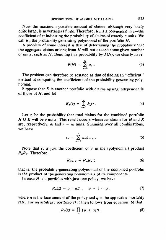
Now the maximum possible amount of claims, although very likely quite large, is nevertheless finite. Therefore, R , is a polynomial in zmthe coefficient of z" indicating the probability of claims of exactly n units. We call R,~ the probability-generating polynomial of the portfolio H.

A problem of some interest is that of determining the probability that the aggregate claims arising from H will not exceed some given number of units, such as N. Denoting this probability by F(N), we clearly have

N

F(N) = Y~ a . . (3)

The problem can therefore be restated as that of finding an "efficient" method of computing the coefficients of the probability-generating polynomial.

Suppose that K is another portfolio with claims arising independently of those of H, and let

Rx(z ) = ~ b.z". (4) n = o

Let c, be the probability that total claims for the combined portfolio H tO K will be r units. This result occurs whenever claims for H and K are, respectively, m and r - m units. Summing o.ver all combinations, we have

c, = ~ a , .b ,_ , , . (5) r,l~O

Note that c, is just the coefficient of z" in the (polynomial) product R , R x . Therefore,

R ~ u x = R u R x ; (6)

that is, the probability-generating polynomial of the combined portfolio is the product of the generating polynomials of its components.

In case H is a portfolio with just one policy, we have

Rn(z) = p + q z " , p = 1 - q , (7)

where n is the face amount of the policy and q is the applicable mortality rate. For an arbitrary portfolio H it then follows from equation (6) that

Rn(z) = [1 (P + q z " ) , (8) H


where the product is taken over the entire portfolio H . Let us now tabulate the portfolio by face amount , w i t h / 4 , denoting

those policies in H with a face amount of n units. We call these H . ' s amount classes and allow for the possibility of amount classes with no members .

Now by propert ies of the logarithm,

where

log R.(z) = ~ log (p + qz") H

(q)] = k Z"' - (9)

~-. Z n k - -

~-, k p

= S , ( z ) - + S : ( z ) + + S ~ ( z ) - . . . ,

In practice the polynomial S,(z) is computed by first computing, for each amount class H. , the sum of kth powers

(11)

and then making a contribution - S.k + S - " to S~(z). • n , k 4~

To compute the probabili ty-generating polynomial of H, we first prove the following:

LEMMA. I f the power series

R(Z) = ~ a,,z" and Q(z) = ~ b,,z" n ~ O n ~ O

are related by

R(z) = e °z~ (12)

DISTRIBUTION OF AGGREGATE CLAIMS 827

on s o m e nontrivial (i.e,, o ther than z = O) interval o f convergence , then the coefficients o f Q and R are related by

and ao = e e° (13)

'2 a. = - ka._kbk , n ~> 1 . (14) n k ~ l

Proof. E q u a t i o n (13) fo l lows b y the subs t i tu t ion o f z = 0 in equa t ion (12). Di f ferent ia t ing (12) wi th r e s p e c t to z y ie lds

R' (z ) = R ( z ) Q ' ( z ) . (15)

W e then obtain formula (14) by equating the coefficients of z" in (15). Our a lgor i thm is based on the fol lowing (see editor's note below):

THEOREM. For k = 1, 2, 3 . . . . let

Q~(z) = s , (z ) - ~S2(z) + ~S~(z) - . . . + - -

R~(z) = eO,~ = ~ a .~z" , a ~ o

( - I), +, S~(z) , (16)

k

(17)

and let Fk(N) be the sum o f the f irs t N + 1 coeff icients o f R~(z), that is,

N

Fk(N) = ~ a . .~ . (181 n=O

Then (i) l im Fk(N) = F ( N ) ,

(ii) F , ( N ) ~ F~(N) ~ . . . ~ F (N) ~ . . . ~ F4(N) ~ F2(N) .

Proof . By equa t ion (9),

(A) l im Q~(z) = log R(z)

so that

( B ) i i m R~(z) = l i r a e e , ~ , = e ,o , Rc~, = R ( z ) .

EDITOR'S NOTE.--An error has been found in the proof of this theorem. The reader should disregard the remainder of this section and read the corrected version in the author's review of discussion.

828 D I S T R I B U T I O N O F A G G R E G A T E C L A I M S

This establishes (i). Let Q(z) = log R(z ) .

IfA(z) and B(z ) are power series, we shall say that A ( z ) <~ B( z ) provided that, for any nonnegative integer N, the sum of the first N + 1 coefficients satisfies the condition

g N

E ao Y, bo. n - O n=O

We have

(D) If atz) ~ B(z) and C(z) <~ D ( z ) .

Then

(DI) A ( z ) + C(z ) <~ B( z ) + D ( z ) ,

(D2) A ( z ) C ( z ) <~ B ( z ) D ( z ) .

Assertion (DI) is immediate. The sum of the first N + 1 coefficients of A ( z ) C ( z ) is

a , ,,c, = c,\g:_o an n ~ 0 k=O k~O

N-k 1

Therefore , A ( z ) C ( z ) ~ B ( z ) C ( z ) . Similarly, B ( z ) C ( z ) = C ( z ) B ( z ) <~ D ( z ) B ( z )

= B ( z ) D ( z ) , so that A ( z ) C ( z ) <~ B ( z ) C ( z ) <~ B ( z ) D ( z ) .

We also have the relation

(E) If A ( z ) <~ B(z), then e A'~' ~ e B'~ .

This last s tatement can be established by applying (D) to the expansion

A ( z ) 2 (El) e A'=, = 1 + A ( z ) + ~ + . . . .

B ( z F e B'=' = 1 + B ( z ) + ~ + . . . .

Note that

(F) Q,(z) <~ Q~(z) <~ . . . ~ Q(z) ~ . . . ~ Q,(z) ~< Q d z ) .

D I S T R I B U T I O N OF A G G R E G A T E C L A I M S 829

This inequality can be established first for the case where the portfolio H consists of a single policy; we may then sum over the entire portfolio H, using (DI). It then follows from (E) that

(G) R l ( z ) <~ R 3 ( z ) ~ . . • ~< R ( z ) <~ . . . ~ R 4 ( z ) ~ R 2 ( z ) .

This establishes part (ii) of the theorem. The algorithm now proceeds as follows:

A.1. Compute the polynomials

Q~(z) = S,(z) - ½S~(z) + . . . + ( - 1)~ +,

Sk(z); (19)

and Qk + i(z) for an odd integer k . A.2. Apply the recursive formula (13), (14) to compute the coefficients

of Rk(z) and R~.,(z). A.3. By the theorem the probability F(N) that claims will not exceed N

units is in the interval

Fk(N) <~ F(N) ~ F,+,(N),

where Fj(N) is the sum of the first N + 1 coefficients of R~(z) for j = k , k + 1.

A.4. Increase the value of k, if desired, for greater accuracy. Since most values of q are low, a single application of steps A.1, A.2, A.3 for, say, k = 5 will generally yield results that are quite accurate (with respect to the assumptions). In any case, few applications of step A.4 are likely to be required.

II1. A N E X A M P L E

In this section we apply the algorithm derived in Section 1I to calculate the aggregate claims distribution of a portfolio of 322 policies ranging in face amount from 1 to 5 units. The example is intended strictly as a conveniently verified simple illustration.

Table 1 shows the classification of the portfolio into amount and mortality classes. Table 2 lists the coefficients of the polynomials Q~(z) defined by equation (19). Table 3 indicates values of Fk(N), the sum of the first N + 1 coefficients of eQg~ calculated by equations (13) and (14). For early values of N we actually calculate eaFk(N) for a convenient value of a.


This device circumvents arithmetical operations with minuscule quantities when the expected number of claims is large. Actual calculations were made to a greater number of significant figures than indicated.

After reading Section IV, the reader is invited to show that, assuming the Balducci hypothesis, the first column of Table 3 describes the aggregate

T A B L E I

C L A S S I F I C A T I O N O F M O D E L P O R T F O L I O BY

M O R T A L I T Y A N D A M O U N T C L A S S E S

FACE AMOUNT DEATHS PER THOUSAND

IN UNITS 0,94 1,91 5.01 13.20 34.07

. . . . . . . . . . . . . 12 23 2 14 20 ! 0 6 7 0

3 1 r i i i i i i i i l l o 3 13 31 o 4 . . . . . . . . . . . . 19 32 24 5 31 5 . . . . . . . . . . . . 6 14 I 36 22

E x p e c t e d number o f c la ims = 4.118

E x p e c t e d units o f aggregate c l a i m s = 14.215

T A B L E 2

COEFFICIENTS OF THE POLYNOMIALS Q~(z)

n Ql(z) Q2(z) ' Q31z) Q4tz) Q~IO

D . . . . . . . . . . . .

l . . . . . . . . . . . .

2 . . . . . . . . . . . .

3 . . . . . . . . . . . .

4 . . . . . . . . . . . .

5 . . . . . . . . . . . .

6 . . . . . . . . . . . .

7 . . . . . . . . . . . .

8 . . . . . . . . . . . . 9 . . . . . . . . . . . . I0 ........... II ........... 12 ........... 13 ...........

14 ...........

15 ...........

16 ........... 17 ........... 18 ........... 19 ...........

20 ...........

21 ...........

22 ...........

23 ...........

24 ...........

25 ...........

-4 .2240129 0 . 9 5 8 0 8 1 3 0 . 1 2 4 7 8 8 2 0.4858726 1 . 3 6 0 2 6 5 0 1 . 2 9 5 0 0 5 8 0 . 0 0 0 0 0 0 0 0.00(30000 0.0000000 0.0000000 0.0000000 0 . 0 0 0 0 0 0 0 0.0000000 0.0000000 0.0000000 0.0000000 0.0000000 0.0000000 0.0000000 0.0000000 0.0000000 0.0000000 0.0000000 0.0000000 0.0000000 0 . 0 0 0 0 0 0 0

-4.1695513 0 . 9 5 8 0 8 1 3 0. I 1 1 0 2 2 0 0.4858726 ! .3595622 1 . 2 9 5 0 0 5 8

- 0 . 0 0 2 9 4 3 6 0.0000000

- 0 . 0 2 0 1 0 1 9 0.0000000

- 0.0169467 0.001301300 0 . ~ 0.0000000 0.0000000 0.0000000 0 .000~00 0.0000000 0.0000000 0.0000000 0.0000000 0.0000000 0.0000000 0 .00000~ 0.0000000 0.0000000

- 4.1706954 0 . 9 5 8 0 8 ! 3 0 . 1 1 1 0 2 2 0 0 . 4 8 6 1 7 6 5 1.3595622 1 . 2 9 5 0 0 5 8

- 0 . 0 O 2 9 3 7 8 0.0000000

-0.0201019 0 . 0 0 0 0 2 5 3

-0.0169467 0.0000000 0 . 0 0 0 4 5 8 5 0.0000000 0.0000000 0.0003506

0.0000000 0,0000000 0.0000000 0.0000000 0.0000000 0.00001300

0,0000000 0.0000000 0.0000000 0.0000000

-4.1706664 0 . 9 5 8 0 8 1 3 0 . I I 1 0 2 2 0 0.4861765 1.3595544 1 . 2 9 5 0 0 5 8

- 0 . 0 0 2 9 3 7 8 0.0000000

- 0 . 0 2 0 1 0 2 0 0 . 0 0 0 0 2 5 3

-0.0169467 0.0000000 0.0004583 0.0000000 0.0000000 0 . 0 0 0 3 5 0 6

- 0 . 0 0 0 0 1 1 9 0.0000000 0.0000000 0.0000000

- 0 . 0 0 0 0 0 8 7 0.0000000 0.0000000 0.0000000 0.0000000 0.0000000

- 4.1706672 0 . 9 5 8 0 8 1 3 0 . 1 1 1 0 2 2 0 0.486 i 765 1.3595544 1 . 2 9 5 0 0 6 0

- 0 . 0 0 2 9 3 7 8 0.0000000

- 0 . 0 2 0 1 0 2 0 0.OOOO253

-0.0169467 0.0000000 0 . 0 0 0 4 5 8 3 0.0000000 0.0000000 0.0003506

-0.0000119

0.0000000 0.0000000 0.0000000

- 0.O000084

0.0000000 0.0000000 0.0000000 0.0000000 0.0000002

T A B L E 3

D I S T R I B U T I O N O F A G G R E G A T E C L A I M S

F R O M M O D E L P O R T F O L I O

N

0 . . . . . . . . . . .

I . . . . . . . . . . .

2 . . . . . . . . . . .

3 . . . . . . . . . . .

4 . . . . . . . . . . .

5 . . . . . . . . . . .

6 . . . . . . . . . . .

7 . . . . . . . . . . .

8 . . . . . . . . . . .

9 . . . . . . . . . . .

10 . . . . . . . . . .

I ! . . . . . . . . . .

12 . . . . . . . . . .

13 . . . . . . . . . .

1 4 . . . . . . . . . .

15 . . . . . . . . . .

1 6 . . . . . . . . . .

17 . . . . . . . . . .

18 . . . . . . . . . .

1 9 . . . . . . . . . .

2 0 . . . . . . . . . .

21 . . . . . . . . . .

2 2 . . . . . . . . . .

2 3 . . . . . . . . . .

2 4 . . . . . . . . . .

2 5 . . . . . . . . . .

2 6 . . . . . . . . . .

2 7 . . . . . . . . . .

2 8 . . . . . . . . . .

2 9 . . . . . . . . . .

3 0 . . . . . . . . . .

31 . . . . . . . . . .

3 2 . . . . . . . . . .

3 3 . . . . . . . . . .

34 . . . . . . . . . .

3 5 . . . . . . . . . .

3 6 . . . . . . . . . .

37 . . . . . . . . . .

38 . . . . . . . . . .

3 9 . . . . . . . . . .

~,1 . . . . . . . . . . .

~,2 . . . . . . . . . . .

~,3 . . . . . . . . . .

i ~,5 . . . . . . . . . .

17 . . . . . . . . . . i

~9 . . . . . . . . . . !

a

! 1 I I I 0 0 0 0 0 0 0 0 0 0 0 0 0 0 0 0 0 0 0 0 0 0 0 0 0 0 0 0 0 0 0 0 0 0 0 0 0 0 0 0 0 0 0 0 0

: F I ( ~ D :F2( N ) :F3(l~ :F~(N) I : F s ( N ) I

.041974 .041976 .039795 .077922 .101152 •131078 •207721 .119082 •152628 •181075 .221389 •277981 .334435 .379795 .425094 .479399 .536760 .586552 •629137 •671821 .715590 .755432 .788703 .817922 .845599 .870925 .892290 .909952 .925297 .938899 .950429 .959783 .967433 .973880 .979271 .983619 .987063 .989830 .992078 .993874 .995274 .996362 .997216 .997885 ,998402 .998794 .999094 .999323 .999497 .999628 .999725 .999798

.042022

.082283 • 106235 • 137282 .217852 • 125028 .159991 • 189359 .231087 .290075 ,348555 .395O01 .441140 .496607 •555156 .605392 .647890 ,690379 .733914 .773227 .805592 .833771 .860379 .884570 .904703 .921111 .935259 • 9477 ! 7 .958148 .966470 .973187 .978797 .983434 .987110 .989971 .992240 .994059 .995489 .996581 .997415 ,998059 .998556 .998931 .999210 .999418 .999575 .999692 .999777 .999839 .999885

• 082189 .106114 .137138 .217627 • 124897 • 159824 .189167 • 230861 •289793 .348215 .394621 .440733 .496162 .554663 .604867 ,647354 .689838 ,73336O .772666 .805043 .833244 ,859873 .884083 .904245 •920690 •934873 ,947363 .957827 ,966185 .972937 .978577 •983242 ,986945 • 989831 • 992120 ,993959 ,995404 • 996511 .997357 •998012 .998518 .998900 .999185 .999399 .999560 .999680 .999768 .999832 .999879

.041976

.082192

.106117

.137142

.217633 • 124900 • 159828 .189172 .230867 .289800 • 348224 • 39463 I .440744 .496174 .554677 .604882 .647369 .689853 .733376 .772683 .805060 .833261 • 859889 .884099 .904261 .920705 .934887 .947377 .957840 .966197 .972948 .978587 .983251 .986953 • 989838 .992126 .993964 .995409 .996516 .997361 • 998015 .998520 .998902 .999187 .999400 .999561 .999681 .999768 .999832 .999879

• 082192 .106117 •137142 •217633 • 124900 .159828 •189172 • 230867 .289800 .348223 • 39463 I .440744 .496174 .554676 .604881 .647368 .689853 •733376 • 772683 .805060 .833260 .859889 .884099 .904260 .920704 .934887 .947376 .957840 .966197 .972947 .978586 .983250 .986952 .989837 .992126 .993964 .995409 .996515 .997361 •998015 .998520 .998902 .999187 .999400 .999561 .999680 .999768 .999832 .999879

831


distribution of claims for the portfolio under the collective Poisson model, with the Poisson parameter equal to the aggregate force of mortality. Thus the collective Poisson model can be regarded as the "first approximation" to the individual model.

IV. PARALLELS WITH THE COLLECTIVE CASE

A. It is now assumed that the reader is familiar with the Society's study note on risk theory [3]. It is straightforward to verify that the generating function of the frequency distribution,

f ( x ) = p*"(x ) - - , (20) .=o n[

of a compound Poisson process is

where

R ( z ) = eO" , (21)

Q(z) = h P ( z ) - k (22)

and P(z ) is the generating function of p(x) . We define

l o g f = Q(z) (23)

and note that if g is the frequency function of another compound Poisson process, then so is f * g, and

l o g ( f *g) = log f + l o g g . (24)

Intuitively, the convolution operation * corresponds to combining port- folios. If I = l (x) denotes the frequency function of the compound Poisson process for the e m p t y portfolio,

then

i(O) = 1 , (25)

l(x) = O, x > O ,

f * ! = l , f = f , (26)

so that I(x) acts as unity if convolution is thought of as multiplication.

DISTRIBUTION OF AGGREGATE CLAIMS

Define l / f to be the function whose generating function is

llR(z) = e -O(z) ,

833

(27)

where (27) is evaluated using the recursive relation given in equations (13) and (14). Then

f * (I/j") = 1. (28)

Letting

f ig = f * (l/g) , (29)

we can define a "division" with respect to the convolution operation, with the caveat that l / fneed not be a probability distribution. Calculations is this system can be performed by addition and subtraction of power series by virtue of formula (24). (The reader who is so inclined can for- mulate this discussion in terms of isomorphic Abelian groups.)

The algorithm is Section III can now be regarded as calculating suc- cessive values of the sequence f~/g~, where f~ and gk are frequency functions of certain compound Poisson processes, the quotient is with respect to convolution, and

lim ~ / g k ) = f i g . (30)

The distribution of aggregate claims for the individual model is the q u o t i e n t f l g ; f a n d g are distributions of compound Poisson processes with parameters h and p(x), where

h. = ~o 2 y , (31) Hy X

h = ~ h~, (32) x = l

and p(x) = hJh. (33)

Here, in the outer sum in (31), D indicates that the sum is taken over all divisors o fx such that x/y is odd ( fo r f ) and even ( for g).

B. Formula (20) may be generalized as

f(x) = ~ s(n)p*~(x), (34) n~o


where s(n) is an arbitrary distribution on the collection of nonnegative integers--usually referred to as a counting distribution. If S(z) is the generating function of s(n), then it is easily verified that

R(z) = S(P(z)). (35)

Frequently, s(n) is a standard a priori distribution-that may make it possible to evaluate f(x) in terms of (the experimentally determined) p(x). For example, if S(z) satisfies the first-order differential equation

then

dS A(z)--;- + B(z)S(z) + C(z) = O,

az

dR a(P(z))--7- + B(P(z))P'(z)R(z) + C(P(z))P'(z) = 0 ,

az

(36)

(37)

which can be regarded as a first-degree differential equation in R(z). If the functions A(z), B(z), and C(z) are not "too complicated," then it may be practical to solve equation (37) by the method of undetermined coefficients, which, together with an initial value, will recursively produce the coefficients of R(z). For example, if

A(z) = 1, B(z) = - h , and C(z) = 0 , (38)

then we obtain the recursive relation (14) corresponding to the compound Poisson process.

As a second example, consider the relationship for certain constants a and b

s(n)= (a + ! ) s ( n - 1), (39)

satisfied by the Poisson, binomial, negative binomial, and geometric distributions, whose corresponding recursive formula was derived by Harry H. Panjer [2]. Given this relationship, then, equivalently,

A(z) = az - 1, B(z) = a + b, and C(z) = 0 , (40)

and solving equation (37) yields a recursive formula for the distribution of aggregate claims. Other variations on this theme, such as a recursive

DISTRIBUTION OF AGGREGATE CLAIMS 835

formula of the type in (39) but operative for only n >~ N, for a given N, can often be handled by suitable choices of A(z), B(z), and C(z).

C. The essence of this section is not, of course, an attempt to derive all-inclusive general formulas. Rather, it is hoped that the reader is con- vinced that the devices employed in this discussion are not special "tricks" but represent general techniques. What has been done is to use to advantage, in a rather elementary way, to be sure, the structural similarity between different mathematical systems---a fundamental principle of mathematics.

V. REMARKS

In this section a number of admittedly subjective remarks are made on the possible role of risk theory in an individual life model office. A note- worthy fact is that the aggregate claims distribution in the individual model reflects all the mortality information about the underlying portfolio, in the sense that, starting with only the aggregate claims distribution, it is in theory possible to reconstruct the entire scheme of amount classes and mortality rates. This result, which can be verified by proving an appro- priate unique factorization theorem for polynomials, points to a central role for the aggregate claims distribution.

Short-term models incorporating only the mortality risk can be con- structed along the lines of Section III. Such a model could, for example, be of use in monitoring from year to year the ratio of actual to expected claims and would serve as a test of the appropriateness of the company's mortality tables. Short-term predictions of the probable fluctuations in claims and the resulting impact on cash flows could also be based on such a model.

A very difficult problem is the construction of long-term models within a risk-theoretic framework. A starting point could be a counterpart of ruin theory for the individual case; however, in the author's opinion the parallel should not be too finely drawn. From a technical point of view, the author believes that methods of finite combinatorics can be used to greater advantage than in collective risk theory. From a fundamental point of view a realistic long-range model will need to incorporate at least the traditional ingredients of the expense and investment risk and federal income taxes. It is at this point that one is truly in the middle of uncharted waters !

The point of view is frequently_expressed that, for practical purposes, the mortality risk is negligible in proportion to the investment and expense risk and accounts in part, no doubt, for the meager use of risk theory in corporate modeling. This conclusion is based on the sound premise that


the probability of a catastrophic mortality loss precipitating insolvency is small and is overshadowed by other, much more immediate, risks. The conclusion, however, contradicts the fact that, after all, the mortality risk is the fundamental risk that is covered by life insurance, and does not explain the considerable importance generally attached to reinsurance. The paradox is resolved by adopting a going-concern rather than a sol- vency perspective. Large swings in claims may not necessarily bring on insolvency but will wreak havoc with cash flows and the orderly operation of the company. Reinsurance costs are more appropriately viewed as the price to be paid for smoothing year-to-year claim costs rather than insurance against a remote contingency for which a stop-loss type of ar- rangement would be much more efficient. One must therefore look at the entire claims distribution curve rather than just the extreme fight tail--a somewhat different emphasis from that of traditional risk theory.

The preceding remarks are only tentative opinions. Their intent is to stimulate interest in the risk theory aspects of model offices for individual life companies. The development of such a model is proposed as a research problem, with the frank admission that one cannot at this time even ask the right questions with sufficient precision.

VI. ACKNOWLEDGMENT

The author is indebted to John Beekman for his valuable comments on an earlier version of this paper.

REFERENCES

!. BIRKHOFF, GARRETT, and ROTA, GIAN-CARLO. Ordinary Differential Equa- tions. Cambridge, Mass.: Blaisdell, 1969.

2. PANJER, HARRY H. "Recursive Evaluation of a Family of Compound Distri- butions." Astin Bulletin, Voi, XII (1981).

3. Risk Theory. Part 5 Study Note (No. 52-7-82. Chicago: Society of Actuaries, 1981. 4. WHITE, ROaERT E, and GREVILLE, T. N. E. "On Computing the Probability

that Exactly k Out of n Independent Events Will Occur," TSA, XI (1959), 88. 5. WOLFENDEN, HUGH H. The Fundamental Principles of Mathematical Statis-

tics. New York: Actuarial Society of America, 1942.

DISCUSSION OF PRECEDING PAPER

DAVID C. MC INTOSH:

Mr. Kornya's succinct and elegant paper appears likely to become set reading for students preparing to take the Society's examination in risk theory. It is therefore particularly unfortunate that the paper's central theorem should contain a serious mathematical error.

The error occurs in the purported proof of statement (D2). Given

N - k N - k

~] a.~< ~] b. for a l ike{O, 1 . . . . . N}, n~O n=O

it does not follow that

' ) ck a. ~< ~ ck b. k=O \ n = O k=O \ n = O

for arbitrarily chosen real numbers Co, c~ . . . . . cN. Mr. Kornya seems to be assuming that Co, Cl . . . . , C;v are all nonnegative, a condition which does not apply to the coefficients of the polynomials Qk(z).

In fact, if we consider a portfolio with only one member, it is evidently false that

[Ql(z)] 2 ~< [Q2(z)] z,

even though it is true that

Ql(z) <~ Q2(z).

Consequently, statement (D2) is invalid in the situation where Mr. Kornya wishes to apply it. (The partial ordering of real power series is that defined by Mr. Kornya for use in his proof.)

Of course, statement (D2) is merely an incidental step in the purported proof of statement (E). Statement (E) is not true for arbitrarily chosen real polynomials A(z) and B(z), and afortiori it is not true for real power series in general. In order to see this, consider

837


1 7 A(z) --- loge2.7 - ~ z + ~ z 2,

B(z) = 1.

It is evident that A(z) <~ B(z), since 2.7 < e and 7A6 < 1/2. However, the third partial sums of coefficients of e a~) and e n~z) are, respectively, 2.86875 and e. Therefore, since 2.86875 > e, it is not true that e A~-') ~< e Bt~).

In order to determine whether part (ii) of Mr. Kornya's theorem is or is not true, it is necessary to establish whether or not statement (E) is true in the case where A(z) = Qk(Z) and B(z) = Qj(z) for some positive integers k and j . This would require analysis of the particular polynomials Qk(z), the series Rk(z), and the sums Fk(N). Mr. Komya 's reasoning, involving general power series, simply is not valid.

In fact, it is not difficult to show that, for a given N, the sequence Fk(N) falls into the desired pattern of alternately monotonic convergence toward F(N) when k /> N (see below for a proof). Unfortunately, this result is too weak for the application that Mr. Kornya wishes to make. For that application it is necessary that the alternating pattern should be followed for all k i> 1, even when N is a large amount. Mr. Kornya's numerical example suggests that the stronger result may indeed be true, but it remains unproved.

To prove the relatively weak result, let us adopt the following notation for a portfolio H: for each h ~ H, write

n h = Face amount of policy h (a positive integer);

qh = Probability of claim under policy h;

Ph = 1 -- qh;

rh = qh/Ph.

For each positive integer m,

a m ( Z )

R(z)

hd-/ h ~ /

= = S , . ( z ) t ~ O m ~ l m

= S i n ( z ) m I m

for al lk>~ 1.

D I S C U S S I O N 8 3 9

Therefore, for all positive integers k,

= R(z) exp Sin(z) R d z ) ,,,= l m

= exp ~ ~ R(z) x m ~ k + 1 m h d t

exp - ~ r~h Z mnh • m ~ k + 1 m hd-/

Now, R(z) = ao + a l z + . . . + a~z a' + terms of greater order than z k. Using the methods described on pages 179-81 of Ahlfors [1], it can be shown that

exp - ~ ~ z ' " h m=k+l m hd~

terms of greater order than ~ ,

= 1 +

and hence that

Rk(z) = exp ~ m=k+l m hal-/

X

(a o + a l z + . . . + ak za' + terms of greater order than zk).

Therefore, for all N ~> 1 and for all k i> N,

It follows, by considering the alternately monotonic convergence to zero of the sequence

,,: Z (-1)°+'Z¢, r a ~ k + 1 m h ~

that the sequence Fk(N) follows the desired alternating pattern of convergence to F(N) when k >t N.

As a final comment, it is worth noting that the various series in Mr.


Kornya's paper are divergent if qh > 1/2 for some policy h e H. Extremely high risks must therefore be excluded from the portfolio before applying the algorithm described in the paper.

REFERENCE

1. AHLFORS, LARS V. Complex Analysis, 2d ed. New York: McGraw-Hill, 1966.

DONALD P, MINASS1AN:

If R ( z ) - ~ anZ n is the generating function for the number of unit claims, n=O

N

then F(N) ~ ~ a,, is the probability that the number of unit claims does n=O

not exceed N. Further, if Rk(z) =-- e ° ~ ) - - ~.~ an,kZ n and if Fk(N) ---- n~O

N

~ . an,k, the question has arisen whether we can have monotonic conver- n=O

gence, that is, specifically whether

Fi(N) <~ F3(N) ~< . . . ~< F(N) ~< . . . ~ F4(N) ~ Fz(N) , (1)

since Fk(N) can readily be calculated for small k (see Kornya's paper). For future reference, this result would follow from

R l ( z ) <<- R3(z) ~< . . . ~< R(z) <~ . . . ~ R4(z) <~ R2(z), (la)

where ~< is as defined below. In this discussion we show (A) that the general answer is no (counterex-

amples are provided) and (B) that there is a monotonic convergence theorem but the algorithm is somewhat more complicated, and convergence slower, than is the case with the original Kornya algorithm. We omit empirical studies of the latter result, but hope that the algorithm will be so tested by others.

A . C o u n t e r e x a m p l e s to Fo rmu la (1)

We present the development of this result, rather than simply the result itself, because it was the inspiration for Part B of this discussion.


We repeat a definit ion used by Korrtya,

Definition. If A(z) =- ~ a.z ~ and B(z) -- ~ bnz ~, then we say A(z) n - O n - O

N N

B(z) if, for every nonnegat ive integer N. we have ~ a . ~ ~ bn. n 0 n O

N

(The motivat ion is that in the series for R(z) =- ~'~ anz n the probabili ty F(N) n - O

N

that the number of unit claims does not exceed N is ~'~ an.) n = 0

PROPOSITION 1. Let A(z), B(z), and ~ be as in the definition. Then A(z) ~ B(z) if and only if, as power series, A(z)/(1 - z) ~s B(z)/(1 - z), where ~ . (s for "s trong") means that each coefficient of A(z)/(l - z) does not exceed the corresponding coefficient of B(z)/( l - z). In fact, a much stronger

N

result holds." for any fixed nonnegative integer N, ~ an does not exceed n ~ O

N

~ bn in the original series A(z) and B(z) if and only if the Nth coefficient n 0

of A(z)/ (1 - z) does not exceed the Nth coefficient ofB(z)/( l - z).

N

Proof. The Nth coefficient of A(z)/(1 - z) is precisely ~'~ a.; similarly r! 0

for B(z)/(1 - z).

COROLLARY I. I f Oi(z) and 0 /2 ) are any m'o power series, then as power series e Oi~:~ <~ eOJ ~:~ if and only if

exp [Qi(z) + z + (z2/2) + (z3/3) + . . . ]

exp [Qj(z) + z + (z2/2) + (z3/3) + , , , ]

(2)

(where in general eC~")-~ ~ [C(z)]"/n!; we assume we are within the radius t! =0

of convergence for C(z), so order of terms is immaterial).

Proof. The expression on the left is

eQi~:) - log¢l - :) = eOi~:)/eiog, i - :~ = eQi~:~/(l _ z). (2 ')

Similarly this is for the expression on the right.


Now consider Ql(z) and Q3(z), with definitions as in Kornya's paper. While it is true that Ql(z) <~ Q3(z), the crucial question respecting formula (1) above is whether e t21~z) ~< e t23(z). By Corollary 1, this holds if and only if formula (2) holds where we take Qi(z) - Ql(z) and Q~(z) =- Q3(z). We further note (calculational details omitted):

LEMMA. I f C(z) -- ~ ciz i is any power series inside its radius o f conver- i=o

gence and i f e ctz) =- ~ ei zi, then i=o

eo = e ¢° el = (1 + cOeCO

e2 = (c~ + 2!c2)e"O/2!

e3 = (c 3 + 6ctc2 + 3!c3)eC°/3! e4 = (c 4 + 12c~c2 + 24clc3 + 12c 2 + 4!c4)eco/4!.

(3)

(Note: at this point we require only the expression for e2; we include the rest for future reference.)

Now let A(z) -- aiz' represent the exponent on the left-hand side of i=o

formula (2), where Ql(z) replaces Qi(z), and let B(z) -- ~ biz i represent i=o

the exponent on the right, where Q3(z) replaces Qj(z). Were e Qltz) e Qa~z), then formula (2) would hold, where Ql(z), Qa(z)replace Qi(z), Qj{z). So, by the lemma,

" e 2 for e Oj~z)'' does not exceed "e2 for eO3(zP'; i.e., (4)

Now assume a portfolio of insureds where each insured has precisely one unit of insurance. Then Q j(z) lacks the quadratic tenn. Hence (compare Komya) a 2 (which is the coefficient from adding (z2/2) to the quadratic ternv--cf, formula (2)) is 1/2. Also, in this case b I = al = 1 + Y. (q/p); b 2

= 1//2 _ _ 1/2 ~ (q/p)2; and bo - ao = t/2 ~ (q/p)2 _ 1A ~, (q/p)3. Multiplying both sides of formula (4) by 2e -a° and using the expressions above, we see that (4) is equivalent to

DISCUSSION 843

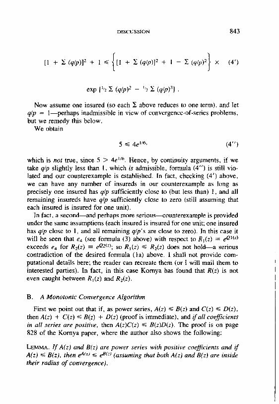
[1 + ~i,(q/p)]2 + 1 ~<{[1 + ~ (q/p)]2 + 1 _ ~,(q/p)2} × (4')

exp [),2 ~ (q/p)2 _ ',3 ~ ( a l p ) 3 ] .

Now assume one insured (so each E above reduces to one term), and let q/p = l--perhaps inadmissible in view of convergence-of-series problems, but we remedy this below.

We obtain

5 ~< 4e 1/6, (4")

which is not true, since 5 > 4e 1/6. Hence, by continuity arguments, if we take q/p slightly less than 1, which is admissible, formula (4") is still vio- lated and our counterexample is established. In fact, checking (4') above, we can have any number of insureds in our counterexample as long as precisely one insured has q/p sufficiently close to (but less than) 1, and all remaining insureds have q/p sufficiently close to zero (still assuming that each insured is insured for one unit).

In fact, a second--and perhaps more serious--counterexample is provided under the same assumptions (each insured is insured for one unit; one insured has q/p close to l, and all remaining q/p's are close to zero). In this case it will be seen that e4 (see formula (3) above) with respect to Rl(z) - e O~(z) e x c e e d s e4 for R2(z) - - eQ2(z); SO RI(g ) ~ R2(7, ) does not hold--a serious contradiction of the desired formula (la) above. I shall not provide computational details here; the reader can recreate them (or I will mail them to interested parties). In fact, in this case Komya has found that R(z) is not even caught between Rl(z) and R2(z).

B. A Monotonic Convergence Algorithm

First we point out that if, as power series, A(z) <<- B(z) and C(z) ~ D(z), then A(z) + C(z) <~ B(z) + D(z) (proof is immediate), and if all coefficients in all series are positive, then A(z)C(z) ~ B(z)D(z). The proof is on page 828 of the Komya paper, where the author also shows the following:

LEMMA. I f A(z) and B(z) are power series with positive coefficients and if A(z) <- B(z), then e Atz; <<. e ate) (assuming that both A(z) and B(z) are inside their radius of convergence).

8 4 4 D I S T R I B U T I O N O F A G G R E G A T E C L A I M S

Now assume for the moment that all coefficients in the exponents of (2) are positive except for the constant term (see Kornya's definition of Qi(z)). We discuss the validity of this "posit ivi ty" assumption below. Let Ai(z) and Aj(z) represent the power series for the exponents of (2). Now, for any two power series, C(z) <~ D(z ) if and only if kC(z) <~kD(z) for any positive constant k. Thus e a;~-') <~ eaJ t~) if and only if, for any real r, e r + Ai(z) e r + aj~z). Hence, by taking r large enough, we may assume that the constant terms of r + Ai(z) and r + Aj(z) are positive. Hence, by our assumption that all other coefficients of Ai(z) and Aj(z) are positive, we may assume that all coefficients o f Ai(z) and Aj(z) below are positive. Now, following Kornya we note that

Q~(z) <~ Q3(z) ~< . . . <~ Q(z) <~ . . . < - Q4(z) <~ Q2(z), (5)

and hence

Al(z ) ~< A3(z ) ~< . . . ~< A(z) <~ . . . < ~ A4(z ) ~ A2(z) (5')

in view of the additive property of <~; (recall that each Ai(z) = Qi(z) - log (1 - z)). Thus, since we assume that each coefficient of each Ai(z) is positive, we have, from the Lemma,

e Al (z ) ~ e A3(z) ~ . . . ~ e A(z) ~ . . . ~ e A4(z) ~ e A2(z) , ( 6 )

or, equivalently, using the Kornya notation (Ri(z) - e Q i ~ z ) ) ,

Rl ( z ) R3(z) R(z) R4(z) R2(z) - - <~ <~ . . . <~ ~< . . . ~< ~ - - ( 6 ' ) 1 - z I - z 1 - z 1 - z ! - z

This yields our algorithm. For, expanding upon the steps in the Kornya paper (p, 829), we proceed as follows: A. 1. Compute the polynomials Qk(z) and Qk + t (z) for odd integer k. A.2. Apply the recursive formula (given by Kornya) to compute the coef-

ficients of Rk(z) and Rk+ t(z). A.3. Calculate the coefficients of Rk(z)/( l - z) and Rk+l(z) / ( l -- z), a

straightforward computation if we recall that the Nth coefficient of A(z) /

( 1 - z) for any A(z ) -- anz n is ~ an. Note that the sum of the first n = 0 n ~ 0

N coefficients of R(z ) / ( l - z) is, by definition of <-, caught between the

DISCUSSION 845

s u m o f the f i rs t N c o e f f i c i e n t s o f R k ( z ) / ( 1 - - z) and R k + l ( Z ) / ( l - z) for

each nonnegative integer N. A.3 . ' Calculate the s u m of the first i coefficients of Rk(Z)/(1 -- z) and

Rk ÷ l(z)/(1 - z) for a l l i = O, 1, 2 . . . . . N (recall that the subscript

for the constant term is zero). Thus, if R ( z ) - ~ rnz ~, and recalling that n=O

i

the ith coefficient of R ( z ) / ( 1 - z ) is ~ r~, we have bounded respectively n~O

r o , r o + (r o + r l ) - - 2r o + r l , ( 2 r 0 + r~) + (r o + rt + r2) -~ 3r0 + 2rl + rE . . . . . (N + l)ro + Nr~ + . . . + rN. From this we can calculate the desired bounds, that is, for r o, r0 + rl , ro + r~ + r 2, etc.,

N

where ~ r~ is the probability that the number of unit claims does not n=O

exceed N. We calculate these bounds by adding (actually subtracting) the inequality bounds for R ( z ) / ( 1 - z) . For example, if a ~< r 0 ~< b and c ~< 2ro + r~ <~ d, then c - b ~< ro + r~ ~< d - a, etc. Similarly, we may calculate bounds for ro + rl + r2, ro + rl + rE + r3, . • • , ro + r~ + r 2 . . . + r N.

A.4. Increase the value of k, if desired, for greater accuracy.

Of course, subtracting the above inequalities diminishes accuracy; i.e., convergence is slowed. At least, however, the accuracy loss accumulates "ari thmetical ly" instead of "geometr ica l ly ." Thus, if our original bounds on the sums of the coefficients o f R ( z ) / ( l - z ) are very tight (as the computer study in the Kornya paper suggests is possible), we may get reasonable accuracy--particularly when the number of insureds is not too great and mortalities are reasonably low. Elementary hand computation shows, for example, that six-decimal-place accuracy in the bounds for R ( z ) / ( l - z)

might achieve two- or three-decimal-place accuracy in the bounds for R ( z ) - -

accuracy sufficient for many applications. Finally, how reasonable is the supposition that all coefficients in the power

series for each Qi( z ) - log (1 - z) are positive (except the constant term)? Recall that we assumed this in our algorithm.

First, if this is n o t so, we can continue dividing by 1 - z until we find an n such that all coefficients (first degree and higher) for

eQi(z)

(1 - z ) n _ _ ~ e Q ~ z ) - n log(l-z) = eQi(z)+nz+(nz2/2)+ . . . (7)

are positive. Indeed, we can find a single n that works for a l l Qi ( z ) and for


Q(z) , since the Qi(z) converge uniformly to Q(z) and since the coefficients of Q(z) are bounded (the series for Q(z) converges for z = 1) if---as assumed tacitly by Kornya---each q/p < 1; thus, with only a finite number of q/p 's , the q /p ' s are bounded away from 1.

Having found such an n, we find, in order, bounds for R(z) / ( l - z)", R(z)/(1 - z ) " - i . . . . . R(z) / ( l - z), R(z) , using the methodology described above. Now clearly the speed of convergence lessens "geometrical ly" as n increases, so we do not wish n to be very large!

Second, returning to the desirable case n = 1, we can point to some fairly realistic situations where all coefficients (except the constant term) for each Qi(z) - log (1 - z) and for Q(z) - log (1 - z) are positive.

Except for the constant term, the largest (in absolute value) possible negative coefficient in any Qi(z) is

2 4 6

(8)

whose absolute value is less than that of

2 1 q

(8')

Now let L be the largest q/p, and, using the formula for summing a geometric series, the absolute value of (8') does not exceed that of

I 2 . 1 -- ~(ML )/(1 - t 4) ~ - ~ M L 2, ( 8 " )

where M is the total number of policyholders. (We assume that L is reasonably small, s o L 4 is relatively insignificant.) Now suppose that L ~ 0.001 (as would be the case at most younger ages for annual q), and suppose that the maximum number of units of insurance is 100 (the unit might be $10,000, so that an insured can buy up to $1,000,000 face value). The worst that can happen for any Qi(z) is that all the negatives accumulate in the coefficient for z 2°°. This is "wors t " because the (q/p)2 terms--by far the worst cul- prits--must be included among coefficients for z 2c, where c = 1, 2 . . . . . 100 under our assumption of a maximal 100 units of insurance; further, the coefficients of the - l o g (1 - z) series (which, we recall, is added to the

OISCUSStON 847

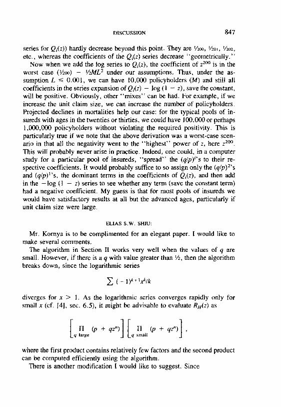
series for Qi(z)) hardly decrease beyond this point. They are 1/2o0, IAo~, V20z, etc., whereas the coefficients of the Qi(z) series decrease "geometrical ly."

Now when we add the log series to Qi(z), the coefficient of z 2°° is in the worst case (½00) - VzML 2 under our assumptions. Thus, under the assumption L <~ 0.001, we can have 10,000 policyholders (M) and still all coefficients in the series expansion of Qi(z) - log ( 1 - z), save the constant, will be positive. Obviously, other "mixes" can be had. For example, if we increase the unit claim size, we can increase the number of policyholders. Projected declines in mortalities help our case: for the typical pools of insureds with ages in the twenties or thirties, we could have 100,000 or perhaps 1,000,000 policyholders without violating the required positivity. This is particularly true if we note that the above derivation was a worst-case scen- ario in that all the negativity went to the "highest" power of z, here z 2°°. This will probably never arise in practice. Indeed, one could, in a computer study for a particular pool of insureds, "spread" the (q/p)i's to their re- spective coefficients. It would probably suffice to so assign only the (q/p)Z's and (q/p)l 's, the dominant terms in the coefficients of Qi(z), and then add in the - log (1 - z) series to see whether any term (save the constant term) had a negative coefficient. My guess is that for most pools of insureds we would have satisfactory results at all but the advanced ages, particularly if unit claim size were large.

E L I A S S . W . SH1U:

Mr. Kornya is to be complimented for an elegant paper. I would like to make several comments.

The algorithm in Section II works very well when the values of q are small. However, if there is a q with value greater than ½, then the algorithm breaks down, since the logarithmic series

( - l)k+ txS,/k

diverges for x > 1. As the logarithmic series converges rapidly only for small x (cf. [4], sec. 6.5), it might be advisable to evaluate Rn(z) as

q large q small

where the first product contains relatively few factors and the second product can be computed efficiently using the algorithm.

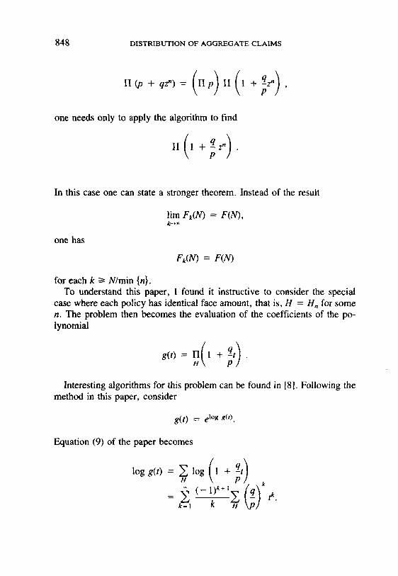
There is another modification I would like to suggest. Since


one needs only to apply the algorithm to find

In this case one can state a stronger theorem. Instead of the result

one has

lira Fk(N) = F ( N ) , k---.~

&(N)= F(N)

for each k I> N/min {n}. To understand this paper, I found it instructive to consider the special

case where each policy has identical face amount, that is, H = Hn for some n. The problem then becomes the evaluation of the coefficients of the polynomial

Interesting algorithms for this problem can be found in [8]. Following the method in this paper, consider

g(t) = e l°g g(t).

Equation (9) of the paper becomes

log /, log(, +q,) k

t*.


If one defines

St = ~ H

then (cf. [5], p. 92, eq. [34])

g(t) = exp (Sit) exp (-$2t2/2) exp ($3t3/3) . . .

= (1 + S i t + $2t~/2! + . . . ) (1 - $2t2/2

+ $2t4/222! - . . . ) . . .

= ~ am tm , ma.O

where

am = ~ ( _ 1)k2+~ . . . . S~' $2 k2 S~ m kl, k2 . . . . . km~,O lk lk l ! 2~2kz! " " " m~mkm!

k l + 2 k 2 + . . . +mkra=m

It is pointed out in Section IV that if a function S satisfies a simple differential equation, then the coefficients of the power series of S(P(z)) can be computed recursively. If S(x) = x ~, et arbitrary, then the resulting recursive formula is called the J. C, P . Mi l ler f o r m u l a in the computer science literature (I2]; [3], Theorem 1.6c; [6], pp. 445-46). Formulas such as equations (19) and (23) of [7] and equations (8) and (9) of [1] are particular cases of the J. C. P. Miller formula. The lemma in Section II presents the recursive formula for the coefficients of the power series of S(P(z)) , where S(x) = e~; this result also appears as problem 6 on page 43 of [3] and exercise 4 on page 450 of [6], with the answer given on page 561. Several interesting recursive formulas are given in [1 ].

This paper has provided an interesting introduction to the manipulation of generating functions and power series. For the readers who wish to take a second course on this topic, I would recommend section 4.7 of [6] and chapter 1 of [3],

REFERENCES

1. CHAN, B. "Recursive Formulas for Discrete Distributions." Insurance: Mathematics and Economics, I (1982), 241--43.

2. HENRICl, P. "Automatic Computations with Power Series," Journal of the Associ- ation for Computing Machinery, III (1956), 10-15.

3. Applied and Computational Complex Analysis. Vol. 1, Power Series--


lntegration----Conformal Mapping--Location of Zeros. New York: Wiley-lnterscience, 1974.

4. KELLISON, S. G. Fundamentals of Numerical Analysis. Homewood, IL: Irwin, 1975.

5. KstrrH, D. E. The Art of Computer Programming. Vol. I, Fundamental Algorithms. 2d ed. Reading, MA: Addison-Wesley, 1973.

6. The Art of Computer Programming. Vol. H, Seminumerical Algorithms. Reading, MA: Addison-Wesley, 1969.

7. TiLLEr, J. A. Discussion of "The Aggregate Claims Distribution and Stop-Loss Reinsurance," TSA, XXXI1 (1980), 538-44.

8. WnrrE, R. P., and GREVILLE, T. N. E. "On Computing the Probability that Exactly k of n Independent Events Will Occur," TSA, XI (1959), 88-95.

BEDA CHAN AND PROMOD K. SHARMA*:

Mr. Kornya presented a new, interesting, and useful algorithm for the distribution of aggregate claims. In this discussion we review two traditional algorithms.

The traditional way of computing the aggregate claims distribution is by convolution [l]. We use the example in Setion III of Mr. Kornya's paper for illustration.

For Table l of the paper, let

nij = Number of policies in row i, column j; qj = Mortality rate for policies in column j; Nij = Number of claims arising from nij; S = Total amount of claims.

Then

Nij ~ Binomial (nij, qj),

and

5 5

s- EZiN,j. i - l j - i

The aggregate claims distribution computed by convolution is given in the second column of Table 1 of this discussion. In our computation, we modify * Mr. Sharma, not a member of the Society, is an honor actuarial science student at the University of Western Ontario.

DISCUSSION 851

the APL programs supplied in [3]. Our figures agree completely with Mr. Kornya's Table 3, last column.

m In convoluting two probability vectors {Pil ~ Pi = 1, Pi ~ 0} and

n { q j | ~ qj = 1, qj >~ O} using APL , an (m + 1) × (n + 1)matr ixisformed.

j=O'=

In a small-size example such as the one illustrated here, the matrix has grown too large to fit into the workspace after a few convolutions. We solve this problem by truncating the probability vectors. The truncation error is held under control by the following propositions. Proposition 1 states that the error of a truncation is bounded by the sum of the truncated tails. Proposition 2 gives a bound on the size of the tail of a binomial distribution.

m n Proposition 1. L e t p = {Pi}i=o ~ Pi = 1, Pi ~ 0}, q ~ {qJ~ --~0':~ qj = | ' qj

t> 0}, f f = {p,[i = 0 . . . . . ~ with ~ <~ m}, and t l = {qj~ = 0,

. . . . "~ with ~f <~ n}. Then

and

(P*q)k ~> (P*'q)k

m+n ~ n Y~ [(P*q)k - (~'*i/)k] ~< Pi + ~ q j .

k~O i ~ + 1 j = ~ + l

Proof. Straightforward, by using the definition of convolution and the fact that p and q are probability vectors.

Proposition 2.

y. pk (1 - p) , -k k=r

p F ( n + 1)

= F(r)F-(n - r + 1) xr - I (1 _ x )n-rdx < pr .

Proof. The equality is from [2; p. 173, problem 45]. The inequality requires using (1 - x) n-r ~< 1 for 0 ~< x ~< p, and integration.

One traditional way of approximating the aggregate claims distribution is by fitting a normal distribution. Note that

8 5 2 DISTRIBUTION OF AGGREGATE CLAIMS

5 5 5 5

E(S) = • Y. iE (N o) = E Y. iniyqj = 14.21462, i=1 j = l i=1 j = l

5 5

Var (S) = X X i 2 Var (Nij) i ~ l j = l 5 5

= • X i2niyqj(l -- qj) i=1 j = l

= 56.9594007622.

The approximation by a normal distribution with matching mean and vari- ance is displayed in column 3 of Table 1 of this discussion.

We share Mr. K o m y a ' s view that risk theory computation should be applied more often. One reason for its infrequent use is probably the volume of computation needed for convolution. Indeed, in a small-size example such as the one considered here, FORTRAN requires a long time for looping and APL requires very large workspace for huge matrices. Our solution here is to truncate the probability vector. Mr. Kornya 's elegant solution is to con- struct a sequence Fk squeezing the true distribution F. If a rough, quick answer is desired, one may use the normal approximation. Compare columns 2 and 3 in Table 1,

REFERENCES

!. BOWERS~ N. L., JR:; GERBER, H. U.; HICKMAN, J. C.; JONES, D. A.; AND NESB1Tr, C. J. Society of Actuaries study note "Actuarial Mathematics." Chicago: Society of Actuaries, 1984.

2. FELLER, W. An Introduction to Probabili~ Theo~' and Its Applications. 3d ed. New York: John Wiley & Sons, 1968.

3. GRENADER, U, Mathematical Experiments on the Computer. New York: Academic Press, 1982.

D I S C U S S I O N

TABLE 1

853

Aggregate Claims

0 1 2 3 4

5 6 7 8 9

10 11 12 13 14

15 16 17 18 19

20 21 22 23 24

25 26 27 28 29

30 31 32 33 34

Cumulative Distribution

by Convolution

.015442

.0302366

.0390382

.0504517 •0800628

•1249 .159828 .189172 .230867 .2898

•348223 .394631 .440744 •496174 •554676

.604881 ~647368 .689853 •733376 .772683

.80506 •83326 •859889 •884099 .90426

.920704

.934887 •947376 •95784 .966197

•972947 •978586 •98325 .986952 •989837

Cumulative Distribution by Normal

Aproximation

.345938D - 01 • 46O239D - 0 i • 603081D - 0 i • 778487D - 0 I • 990138D-01

• 124109D 03 • 153345D 00 • 186816D 03 • 224468D 03 .266088D 00

• 311293D 03 .359540D 00 .410139D 03 .462282D 03 .515082D 03

.567618D 03 • 618984D 00 .668333D 00 • 714920D 03 .758135D 03

.797526D 03

.832807D 00

.863858D 00

.890711D 00

.913530D 03

.932584D 03

.948218D 03

.96O823D 03 • 970809D 03 .978583D 03

• 984529D 00 .988999D 00 • 992303D 03 • 994696D 03 .996404D 03

Aggregate Claims

35 36 37 38 39

40 41 42 43 44

45 46 47 48 49

50 51 52 53 54

55 56 57 58 59

6O 61 62

Cumulative Distribution

by Convolution

.992126 •993964 .995409 • 996515 •997361

•998015 .99852 .998902 .999187 .9994

• 999561 • 99968 .999768 .999832 .999879

• 999914 .999939 .999956 .999969 .999978

.999985

.999989 • 999993 •999995 • 999996

.999997 • 999998 • 999999

Cumulative Distribution by Normal

Approximation

.997601D 03 • 998426D 00 .998983D 00 .999354D 03 .999596D 03

.999752D 00 • 999850D 03 .999911D 00 .999948D 03 .999970D 03

.999983D 03 • 999991D 00 .999995D 03 .999997D 00 .999999D 03

.999999D 03

. I ~ D 01

.100000D 01

.100300D 01

.100303D 01

.100(K~D 01

.100000D 01 • 100030D 01 .100303D 01 .100000D 01

.100000D 01 • 1 0 ( 0 ) O D 01 • I ~ D 01


( A U T H O R ' S R E V I E W O F D I S C U S S I O N )

P E T E R S. K O R N Y A :

I would like to thank the discussants for their stimulating comments . I am indebted to Mr. Mclntosh for pointing out the error in the proof o f

the theorem and for giving me the opportunity to correct it. The reader should disregard the theorem in Section II and replace it with the following:

THEOREM, Suppose that q<~ ½ for each policy in the portfolio H and f o r k = 1 , 2 , 3 . . . . let

and

1 ( - 1) k+l Q~(z) = S1 (z) - ~ S 2 ( z ) + . . . + ~ Sk(z) , ( 1 6 a )

Q(z) = lira Qk (z) = log R(z), (16b) k- - .~

Rk(z) -: e a~=' = ~ a,.k z n, (17) n = 0

N

fk(N) = ~] [a,.k}, (18) n - - 0

k + l

e - k + l "

then

IF(N) - Fk(N)I ~ e ' - - 1 (i)

and

lira Fk (N) = F(N). (ii)

Proof. If A(z) and B(z) are power series, say that A(z) <~ B(z) provided that, for any nonnegative integer N, the sum of the first N + 1 coefficients satisfies

N N

Z a. b.. (A) N = O n ~ O

DISCUSSION

Also define IA(z)l to be the power series

IA(z)l = ~ la.lz". n=O

855

(B)

Then it is easily shown that

A(z) <~ ~4(z)J, (CI)

IA(z) + B (z)l -< IA(z)l + IB(z)l, (C2)

Ia(z) BU)I ~ IA(z)l IB(z)l. (C3)

If IA(z)l ~< Ia(z)l and IC(z)l ~< IDU)I, (C4)

then IAU)I IC(z)l <~ IB(z)l IV(z)l,

and, using equations (13) and (14), we have the following:

(C5)

Note that an arbitrary constant can be regarded as a power series with all but the first term equal to zero. Then, using (C1), (C2), (C3), (C4), and (C5), we have the following: Ia(z) - Ok(z)[

-- I E 2 ( - ' ) " ' q ( -

~', i ~, (--1)k÷J q 1 2n(k +j) j= I k ' ~ (D)


k + l k + l

k + l

q <~ 1/3 is used in the last step. Now note that

IR(z)l = IRx.(z) e Q'=) - Qk(=)l <~ IRk(z) I elQ¢=)-Qk(=)l, (E)

so that

F(N) ~< F k (N)e ~. (F)

Similarly,

Fk(N) <~ F(N) e~; (G)

therefore,

Fk(N) - F(N) ~< (e" - 1) F ( N ) <~ e ' - i (H)

and

F ( N ) - F k ( N ) <~ (1 - e-') F(N) ~< 1 - e ' " ~< e ~ - 1, (I)

from which (i) follows. Statement {ii) is an immediate consequence of (i). The algorithm now proceeds as follows:

A. 1. Choose a value of k for which the magnitude of error

e ' ~ - l

is sufficiently small. A value of k = 5 will, for a typical insurance portfolio of several hundred thousand policies, generally yield results accurate to the fifth decimal place. A.2. Compute the polynomial Qk (z) and apply the recursive formulas (13)

DISCUSSION 857

and (14) to compute the coefficients of Rk(z). By the theorem, a conservative estimate for the distribution of aggregate claims is

F(N) <~ Fk(N) + e e - 1.

Dr. Minassian has pointed out that it is not necessarily true that

FI(N) ~< F3(N ) ~< . . . ~< F(N) ~ . . .~ F4(N ) ~< F2(N). (J)

His counterexamples saved me from heroic attempts to prove the original version of the theorem. As far as the algorithm is concerned, however, the inequality (J) is not really necessary--all that is needed is an efficient bound on the error ]F(N) - F~(N) I. There is no need to modify the algorithm described in Section II.

Dr. Shiu and others point out that values of q must be small for the algorithm to work well. Although q < i,~ is the absolute requirement for convergence, the values of q should be considerably smaller for efficient convergence. The algorithm is intended to apply to a typical insurance portfolio with a one year horizon where the q's are generally quite small. Taking k = 5, for example, the algorithm evaluates the claims distribution to within six decimal places for a portfolio of 322,000 policies distributed according to the example in Section III. His suggestion to partition the portfolio into subportfolios can be extended to partitioning by other categories, such as male/female, standard/substandard, etc. The suggested modification for which

F(N) --- Fk(N) (K)

is, I believe, of limited practical importance because of the large value of k generally required. In the example just cited, one needs k = 14,215 just to ensure equality up to the expected amount of claims. The suggested algorithm is in fact tantamount to an exact evaluation of the coefficients of the polynomial R(z).

Dr. Shiu lists many excellent references, to which I would like to add one more. The algorithm described in Section II is really nothing but Newton's formula for the relationship between the coefficients and the sums of powers of the roots of a polynomial.

Dr. Chan and Mr. Sharrna give an alternative method of computation by direct convolutions, with truncation of the tail end of the distribution to cut down on the volume of computation. This method, I suspect, still involves


a considerable amount of computation in order to suitably approximate port- folios with a substantial number of policies. In such a case, their suggestion of using the normal distribution may work quite well in view of the convergence of the binomial to the normal distribution. A useful result would be a practical bound on the degree of error in the normal approximation to the aggregate claims distribution.

distribution of aggregate claims in the - … · transactions of society of actuaries 1983 vol. 35...

Documents